terrestrial planet finder interferometer tpf-i · pdf filejpl document d-38839 terrestrial...

JPL Document D-38839

Terrestrial Planet Finder Interferometer TPF-I Technology Milestone #1 Report Editors: Robert D. Peters, Peter R. Lawson, and Oliver P. Lay July 24, 2007 National Aeronautics and Space Administration Jet Propulsion Laboratory California Institute of Technology Pasadena, California

JPL Document D-38839 TPF-I Technology Milestone #1 Report

- ii -


- iii -

Approvals Released by ____________________________________________ _________________ Robert D. Peters, TPF-I Adaptive Nuller Cog. E. Approved by ____________________________________________ _________________ Peter R. Lawson, TPF-I Systems Manager ____________________________________________ _________________ Daniel Coulter, TPF Project Manager JPL ____________________________________________ _________________ Charles Beichman, TPF Project Scientist, JPL ___________________________________________ _________________ Michael Devirian Navigator Program Manager, JPL ____________________________________________ _________________ Zlatan Tsvetanov TPF Program Scientist, NASA HQ ____________________________________________ _________________ Lia LaPiana TPF Program Executive, NASA HQ


- iv -

Table of Contents

Approvals............................................................................................................iii

Table of Contents............................................................................................... iv

1. Abstract ...........................................................................................................1

2. Introduction ....................................................................................................1

2.1. Lab Demonstration ......................................................................................................3 2.2. Differences between Flight and Lab Demonstration .............................................6

3. Milestone Procedures..................................................................................... 6

3.1. Definitions .....................................................................................................................7 3.2. Measurement of the null..............................................................................................8 3.3. The M1 Validation Procedure ....................................................................................8

4. Success Criteria .............................................................................................. 9

5. Lab Results....................................................................................................10

5.1. Data Acquisition .........................................................................................................11 5.2. Intensity correction ....................................................................................................11 5.3. Phase correction .........................................................................................................13 5.4. Nulling test ..................................................................................................................15 5.5. Stability .........................................................................................................................17 5.6. Throughput..................................................................................................................21

6. Conclusions ...................................................................................................21


- 1 -

Terrestrial Planet Finder Interferometer

TPF-I Technology Milestone #1 Report Amplitude and Phase Control Demonstration

1. Abstract This document reports the achievement of TPF-I Technology Milestone #1, a demonstration of broad spectrum quasi-static control of intensity and phase of interfering beams for deep broadband nulls. We review the milestone specification from the Milestone White Paper (December 18, 2006), summarize the experiments performed in the Adaptive Nulling Testbed, detail the procedures and analysis of the resulting data, and describe and present the data itself.

2. Introduction Direct detection of Earthlike planets around nearby stars requires a combination of starlight sup-pression and high angular resolution (< 0.1 arcsec). The technique of nulling interferometry has been proposed at mid-infrared wavelengths for both the European Darwin mission and NASA’s Terrestrial Planet Finder Interferometer (TPF-I).

For a mid-IR interferometer, the light from the star must be suppressed by a factor of 105 or more over the bandwidth of interest, currently 7–17 µm. All designs of TPF-I under consideration include a single-mode spatial filter (SMSF) through which the combined light is passed before being de-tected. The wavefront from the star is incident on the collecting apertures of the instrument and de-livered by the respective beam trains to a central beam combiner that couples the light into the SMSF. With just a single mode for each polarization state, the problem of nulling the on-axis light is simplified. The electric field within the SMSF is the vector sum of the electric field contributions from each collecting aperture. The starlight is nulled when the electric fields in the SMSF sum to zero, requiring specific combinations of the electric field amplitude and phase.

The required null depth in turn drives the requirements on the accuracy of the amplitude and phase control. The detection of an Earth-like planet around a sun-like star at 15 pc requires that the elec-tric field amplitudes are matched to within ~0.1% (intensities equal to within 0.2%) and the phase is controlled to ~1 mrad (1.5 nm at a wavelength of 10 µm) simultaneously at all wavelengths and both polarization states. A number of effects can perturb the amplitude coupling into the SMSF including reflectivity, beam shear, and wavefront aberration: tilt, focus, astigmatism, coma, etc. The phase is a function of the optical path length but also changes due to birefringence and dispersion introduced by the ~30 optical elements present in each beam train.

One approach to architecting the instrument is to attempt to make the beam trains as identical as possible by applying very tight requirements to the alignment and specification of the optical ele-ments. Error budgeting shows that the tolerances involved are prohibitive. Our solution is a tech-nique that we call Adaptive Nulling in which a compensator is included in each beam train to correct for imbalances in the amplitude and phase independently at each wavelength and polarization.

The performance of adaptive nulling is described in this report. The goal of the technology demon-stration, as specified in the Milestone #1 White Paper, is as follows:


- 2 -

“Using the Adaptive Nuller, demonstrate that optical beam amplitude can be controlled with a precision of ≤ 0.2% rms and phase with a precision of ≤ 5 nm rms over a spectral bandwidth of > 3 µm in the mid IR for two polariza-tions. This demonstrates the approach for compensating for optical imperfections that create instrument noise that can mask planet signals.”

This goal for phase dispersion and intensity dispersion was chosen to be consistent with a 100,000:1 null depth, which is the flight requirement for TPF-I. A phase mismatch of 5 nm and an amplitude mismatch of 0.2% would yield a null of 100,000:1, if all other sources of null degradation could be made identically zero. This level of performance was deemed to be sufficiently challenging to serve as a convincing demonstration of the viability of adaptive nulling.

The adaptive nuller uses a deformable mirror (DM) to apply a high order adjustment of amplitude and phase independently within the single mode filter. A schematic of the adaptive nuller is shown in Fig. 1, as it would be used to adjust the intensity and phase of one beam in a two-beam nuller. The incident beam is first split into its two linear polarization components, and then dispersed by wavelength. These beams are then directed onto a deformable mirror where the piston of each pixel independently adjusts the phase of part of the dispersed spectrum. Tilt in the orthogonal direction may also be independently adjusted, and, by means of controlled vignetting at a subsequent aperture, provides an independent adjustment of the intensity of part of the dispersed spectrum. The dis-persed spectrum of each polarization is recombined to yield an output beam that has been carefully tuned for intensity and phase in each polarization as a function of wavelength within the single mode spatial filter. If the Adaptive Nuller is used to balance beams entering a nulling interferome-ter, matching tolerances on optical components in that interferometer are substantially relaxed. The ultimate null depth and stability are now determined by the performance of the Adaptive Nuller, under active control that can be monitored (see Sections 3.1.6 and 3.1.8c) and readily characterized, and optical components need only be of sufficient quality that the two arms of the interferometer are matched in intensity and phase to within the capture range of the Adaptive Nuller.

The correction of the amplitude and phase for each polarization and at each wavelength is illustrated in Fig. 2. The piston of the DM adjusts the phase of the output beam (Fig. 2a); changing the local

Figure 1. Schematic of the Adaptive Nuller. Light in one arm of a nulling interferometer is balanced by splitting the polarizations and dispersing the wavelength, then adjusting the phases in each part of the spec-trum with a deformable mirror prior to recombining both polarizations.


- 3 -

slope of the DM at the focal point introduces a shear of the outgoing collimated beam, which is then converted into a reduction of amplitude by the exit pupil stop (Fig. 2b). The piston and local slope are adjusted independently for the different wavelengths and polarizations.

(a) Phase control with piston:(a) Phase control with piston: (b) Amplitude control with tilt:(b) Amplitude control with tilt:(a) Phase control with piston:(a) Phase control with piston: (b) Amplitude control with tilt:(b) Amplitude control with tilt:

Figure 2. a) Side view of phase control with a single wavelength channel on the DM using piston. b) Amplitude control of a single wavelength channel on the DM using tilt. This compensator is part of a control system for balancing the amplitudes and phases of the incom-ing beams. Also needed is a sensor for detecting the imbalances and an algorithm to make the ap-propriate adjustment at the DM. Since we are correcting for imbalances across the science band the sensor must operate over the same range of wavelengths. The amplitudes and phases of the different beams are measured by measuring the photon rate of each arm of the interferometer, and by meas-uring the dispersion when the delay line is moved away from where the null was found. These measurements cannot be done during the science observations which last for several hours. There-fore, the measurements must be done between science observations, and the correction must be stable during the observation. Although this method reduces the time available for science observa-tions, the advantages of this method are that there are no additional sensors needed, there are no uncommon path effects, the amplitude and phase can be measured separately, and the science star is used as the calibration source which avoids changing the pointing of the array.

2.1. Lab Demonstration

Fig. 3 shows the simplified schematic for the mid-IR demonstration. The source shown in Fig. 4 (and described below) generates the light, which is sent through a Mach-Zehnder type interferome-ter. In one arm, we have the adaptive nuller compensator as described above. In the other arm, we have a copy of the adaptive nuller compensator, but with a fixed reference mirror in place of the de-formable mirror. There is also a delay line in the reference arm (not shown) consisting of a large retro-reflector with two levels of actuation. The coarse actuation is accomplished by a computer-controlled linear stage with 50 mm of travel and 0.1-µm resolution. The fine level is done with a PZT actuator, which is coupled with a simple metrology system1,2 to take out air-path variations. Finally, the output is recombined and sent through a SMSF before being detected by a spectrometer.

A schematic of the source is shown in Fig. 4. It consists of a ceramic heater, which is collimated by off-axis parabolas. A small CO2 laser is co-aligned with the white light source to assist in alignment and calibration of the spectrometer. The source also contains a chopper wheel, which allows lock-in detection in the spectrometer. A 75-µm pinhole at the focus between two off-axis parabolas also provides some spatial filtering.

1 F. Zhao, Proceeding of the ASPE Annual Meeting, 345 (2001).

2 P. Halverson, D. Johnson, A. Kuhnert, S. Shaklan, R. Spero, SPIE Proceedings of Optical Engineering for Sensing and Nanotechnology, 3740:646 (1999).


- 4 -

Source

Spectrometer

AdaptiveCompensator

ReferenceCompensator

BeamSplitter

Mirror Single mode fiber

BeamSplitter

Mirror

Source

Spectrometer

AdaptiveCompensator

ReferenceCompensator

BeamSplitter

Mirror Single mode fiber

BeamSplitter

Mirror

Figure 3: Schematic layout for the mid-IR demonstration. The adaptive compensator is in one arm, and a “reference” compensator in the other arm. The reference has all the same optics as the adaptive compensator with the exception of a fixed mirror in place of the deformable mirror.

CO2 Laser

ChopperWheel

Flipper Mirror

CeramicHeater

Pinhole

Off-axisParabolic

Mirror

Output

CO2 Laser

ChopperWheel

Flipper Mirror

CeramicHeater

Pinhole

Off-axisParabolic

Mirror

Output

Figure 4: Schematic of the mid-IR source. Either the CO2 laser or broadband output may be selected by the flipper mirror.

Figure 5: Picture of a MEMS DM used in the demonstration. The small square in the middle is the 3mm x 3mm mirror surface.


- 5 -

In the adaptive nulling compensator, wavelength separation and recombination is accomplished with zinc selenide (ZnSe) wedges with a wedge angle of 7 degrees. In the flight instrument, the light in each polarization would be split with a cadmium selenide (CdSe) Wollaston prism, and subsequently recombined. However these prisms are very expensive, and it was deemed unnecessary to demon-strate the polarization splitting in this testbed. The testbed was intended to operate with either a sin-gle polarization, or to simply pass both polarizations through the system. Because of the limited number of optics we did not expect to see significant polarization effects, and we ultimately chose not to use polarizers. In the experiments described in this report, both polarizations are passed through the Adaptive Nuller without polarization splitting. The setup was modeled in Zemax, which predicted the wavelengths would be spread across ten pixels of the DM.

The adaptive nuller compensator contains the DM as shown in Fig. 5. The actuator we chose was a 3 mm square 12x12 array minus the four corners MEMS DM from Boston Micromachines. The DM consists of a thin gold-coated continuous membrane that is deformed with electrostatic actua-tors driven by a custom 12-bit resolution digital high voltage controller system. The total stroke of any one actuator is approximately two micrometers.

The output of the SMSF is fed into a spectrometer. The spectrometer collimates the light out of the SMSF, and then disperses the wavelengths with a grating blazed for 10 µm. Finally, the light is fo-cused onto an array of sixteen mercury cadmium telluride detectors. The output of each detector is amplified and sent into a multiplexer that allows us to select a single channel to send to the lock-in amplifier for measurement.

To measure the amplitude error, a spectrum of each beam is taken by shuttering the other beam off. We then use the difference divided by the sum of the two spectra as a measure of the intensity im-balance. A positive intensity imbalance indicates more light in the adaptive nuller arm, while a nega-tive imbalance indicates more light in the reference arm. As the adaptive nuller can only decrease the light coupled into the SMSF, we must begin with a positive imbalance. To force the imbalance to be positive, we can use an adjustable iris on the reference arm to decrease the light. Once the im-balance is positive, and the coupling loss vs. tip/tilt angle is calibrated we can apply the appropriate control signals to match the intensities at each particular wavelength. In the flight system, this would not be an issue as each arm would have an adaptive nulling compensator.

Phase dispersion is measured with a variant of the Hilbert transform. This measurement requires the delay line be set a distance away from the null to produce fringes in the dispersed spectrum. The spectrum of the combined light in the interferometer is modulated by fringes whenever the path-difference is non-zero. These have been termed fringes of equal chromatic order and produce a chan-neled spectrum. We measure the fringes in the channeled spectrum with the spectrometer, and the output of our algorithm is a phase error versus wavelength, which is then used to calculate the ap-propriate piston settings for each actuator on the DM. This method has worked very well in previ-ous near-IR experiments; however, it requires the optical path to remain stable as the spectrum is read. Our spectrometer requires several minutes to read the 16 output channels consecutively, so to stabilize the path we implemented an optical metrology system that operates at a wavelength of 1.319 µm.

Some cross coupling is also expected in the form of amplitude correction causing phase dispersion, and vice versa. However, we found that if we iterate between phase and amplitude correction, the two corrections converge after 3 to 5 iterations. The cross coupling may also be decreased by choosing an output aperture that is elliptical instead of circular. This would make the shear in the phase correction direction less sensitive than the shear in the intensity correction direction.


- 6 -

The level of optical path fluctuations due to atmospheric turbulence was reduced with a tarp placed over the interferometer section of the table. No additional insulation was provided, and only the standard room temperature control was used.

2.2. Differences between Flight and Lab Demonstration

There are several important differences between the lab demonstration and the baselined flight im-plementation: 2 beams vs 4 beams, spacecraft dynamics, air vs cryo-vacuum, and the time needed to make a measurement (SNR difference). Each is addressed briefly below. 2 beams vs 4 beams: the X-Array nulling configuration combines 4 beams to form the null. This is implemented in two stages: pair-wise nulling followed by cross-combination of the two nulled beams. Since all the nulling occurs at the first stage, the two-beam lab demonstration provides a meaningful representation. Spacecraft dynamics: a control system is required in flight to stabilize the beams against motions of the spacecraft. It is assumed that the tip/tilt, optical path difference, and shear of each beam is stabilized at the input to the adaptive nuller. The lab demonstration has active path length control only. The active stabilization of 4 beams is demonstrated in the Planet Detection Testbed. Polarization: the flight system will split the two linear polarization states and correct each inde-pendently. The lab demonstration operates on unpolarized light without splitting the components, and therefore has fewer degrees of freedom to make a correction. Cryo-vacuum: the flight system operates in vacuum at low temperature (~ 40 K), compared to the ambient air environment of the lab demonstration. The lab is a more challenging disturbance envi-ronment, and the room temperature thermal background is a significant source of noise in the ex-periment. Future engineering will have to address the need for a DM that operates in vacuum at low temperature. SNR: the broadband source in the lab provides a higher photon flux than the target stars to be ob-served by the mission (the lower effective temperature of the thermal source is more than compen-sated by the much higher solid angle subtended by the source). This is offset by the higher detector readout noise in the lab. The flight system requires approximately 2 s to measure the amplitude to 0.1% in 12 channels across the spectrum for one beam (sun-like star at 10 pc, 3 m collectors). The lab set-up obtains this accuracy for a single channel in ~ 0.3 s of integration, but must repeat the measurement in series for each of the 12 channels. In-flight calibration may require up to 10% of the mission observing time for faint targets. 3. Milestone Procedures Here we collect the various definitions, procedures, and requirements that comprise the TPF-I Technology Milestone #1, as specified in the Milestone White Paper (18 December, 2006).


- 7 -

3.1. Definitions

The TPF-I Adaptive Nuller M1 amplitude and phase control demonstration requires measurement and control of amplitude dispersion and phase dispersion in an interferometer. In the following paragraphs we define the terms involved in this process, spell out the measurement steps, and spec-ify the data products. 3.1.1. “Star”. We define the “star” to be a 75 μm diameter pinhole illuminated with ceramic

heater thermal source with a temperature of 1250–1570 K. This “star” is the only source of light in the optical path of the adaptive nuller. It is a stand-in for the star signal that would have been collected by the telescope systems in TPF-I; however it is not intended to simu-late any particular collector design or expected flux.

3.1.2. “Dispersion”. We define dispersion to be the difference in either amplitude or phase as a function of wavelength between the two arms of an interferometer.

3.1.3. “Algorithm”. We define the “algorithm” to be the computer code that takes as input the measured amplitude and calculated phase dispersion, and produces as output a voltage value to be applied to each element of the DM, with the goal of reducing the dispersion.

3.1.4. “Cross coupling”. We define cross coupling to be the unintended adjustment of phase while amplitude is being corrected or the unintended adjustment of amplitude while phase is being corrected.

3.1.5. “Dispersion free source”. We define a dispersion free source to be a carbon dioxide laser with an operating wavelength near 10 µm with narrow spectral line width that is co-aligned with the “star” source. As we are only able to control dispersion, we do not expect to achieve a null deeper than the null obtained with this source.

3.1.6. “Active metrology”. We define active metrology as a system which uses a laser at 1.3 µm wavelength to measure the difference in optical paths of the two arms of the interferometer. This information is then fed back to the delay line control to maintain a set path difference.

3.1.7. “Spectrometer”. We define a spectrometer to be a device to measure intensity as a func-tion of wavelength. The device consists of a grating to disperse the incoming light. The dispersed light is then focused by an off-axis parabola onto a linear mercury cadmium tellu-ride array with 16 elements. Each element produces a voltage proportional to the intensity in a wavelength range selected by the grating. The output voltages are then sent through a multiplexer to a lock-in amplifier with an integration time set from 100 ms to 1 s depending on the signal level. The output of the lock-in amplifier is then read by the computer for each element of the linear array. Noise may be reduced by averaging up to 10 frames taken from the spectrometer.

3.1.8. “Adaptive nulling”. We define the process of adaptive nulling to be the following 4 step process, iteratively repeated for as many cycles as necessary to reach the desired level of am-plitude and phase dispersion. a) Measure the amplitude dispersion in the interferometer by measuring the intensity spec-


- 8 -

trum of each arm independently while shuttering off the other arm. b) Compute the required tilts to equalize the amplitude difference in each channel of the de-formable mirror (DM) and apply these voltages. c) Calculate the phase dispersion in the interferometer by actuating the delay line several fringes off the null and measuring the dispersed spectral fringes with the spectrometer and applying an algorithm to the output. d) Compute the required pistons to equalize the path lengths in each channel of the DM and apply these voltages.

3.1.9. “Null Depth” the ratio of the peak signal caused by constructive interference in the inter-ferometer to the null signal caused by destructive interference in the interferometer.

3.1.10. “Rejection Ratio” is the inverse of null depth.

3.2. Measurement of the null

Each null measurement is obtained as follows: 3.2.1. The delay line is actuated by the computer to locate the approximate position of the mini-

mum integrated power as measured on the spectrometer. 3.2.2. The delay line is then actuated by the computer to the peak integrated power. The set point

is slowly scanned on the active metrology to locate the peak. The peak integrated power is used to normalize the null depth.

3.2.3. The delay line is then actuated by the computer back to the null. 3.2.4. The metrology set point is then slowly scanned by the computer to find the minimum inte-

grated power as measured on the spectrometer. 3.2.5. The active metrology system can then be used to hold this position to measure the time evo-

lution of the null.

3.3. The M1 Validation Procedure

3.3.1. All DM actuators are set to half their control range. 3.3.2. The active metrology system and the star are turned on. The delay line is then actuated by

the computer to locate the null position. 3.3.3. An initial uncorrected null is measured as described in Sec. 3.2. 3.3.4. The delay line is actuated away from the null by several fringes and adaptive nulling is per-

formed to correct the measured amplitude dispersion to ≤0.2% and correct the measured phase dispersion to ≤5nm.


- 9 -

3.3.5. The delay line is actuated by the computer to locate the null position. 3.3.6. The corrected null is measured as described in Sec. 3.2 3.3.7. The delay line is actuated by the computer several fringes from the null and the phase dis-

persion is calculated and amplitude dispersion is measured. 3.3.8. To measure the stability, step 3.3.6 is repeated while the DM voltages are held constant and

the active metrology holds the delay line position to measure the time evolution of the null. 3.3.9. Step 3.3.7 is repeated while the DM voltages are held constant. Active metrology then holds

the delay line position during the phase calculation to measure the time evolution of the phase and amplitude dispersion.

3.3.10. The source is switched from the star to the dispersion free source and the amplitudes in each

arm of the interferometer are matched. 3.3.11. A dispersion free null is measured as described in Sec. 3.2. 3.3.12. The following data are to be archived for future reference: (a) raw spectrometer output of

null and peak of star before and after correction, (b) phase and amplitude dispersion before and after correction, (c) raw spectrometer output of the null and peak, and phase and ampli-tude dispersion measured at each time interval after correction, (d) raw null and peak data for the dispersion free source.

3.3.13. The following data are to be presented in the final report: (a) Plot showing peak and null as

a function of wavelength before and after correction, (b) plot of time series with RMS and P-V phase and amplitude dispersion, (c) plot of time series of null depth, (d) null depth of dis-persion free source, (e) throughput of the adaptive nuller arm of the interferometer meas-ured with the dispersion free source.

3.3.14. Repeat steps 3.3.1 – 3.3.13 on two more occasions on different days, with at least two days

between each demonstration. 4. Success Criteria The following is a statement of the 6 elements that must be demonstrated to close the TPF-I Mile-stone #1. Each element includes a brief rationale. 4.1 An amplitude dispersion corrected to ≤ 0.2% rms (1σ) over a bandwidth > 3 µm in the 7–12

µm wavelength range starting with a mean error as a function of wavelength of at least 9% between the two arms of the interferometer.

Rationale: This provides evidence that a wavelength dependent amplitude mismatch can be corrected, which cannot be done through traditional methods.


- 10 -

4.2 A phase dispersion corrected to ≤ 5 nm rms (1σ) over a bandwidth of > 3 µm in the 7–12 µm wavelength range starting with a mean error as a function of wavelength of at least 400nm between the two arms of the interferometer.

Rationale: This provides evidence that the wavelength dependent phase mismatch can be corrected. 4.3 Both (4.1) and (4.2) are to be satisfied simultaneously after iterating between amplitude and

phase correction. Rationale: This provides evidence that the cross coupling will not limit the ability to achieve the requirement. 4.4 A peak rejection ratio with the star that is within 10% of the peak rejection ratio of the dis-

persion free source at each spectral channel. Rationale: The dispersion free source tests the fundamental limit of the interferometer’s performance. Adaptive nulling only compensates polarization-dependent amplitude and phase dispersion; therefore, other factors such as path length fluctuations that may limit the peak rejection ratio should be common to both the corrected star and dispersion free source. 4.5 A time series showing deviation of the amplitude and phase to be within the ranges defined

in (4.1) and (4.2) for a 6 hour period while the DM control voltages are held constant. As was done in the proof-of-concept demonstration, room temperature will be monitored but not controlled beyond the facility controls for the room.

Rationale: The adaptive nuller is a quasi-static correction that cannot be changed during an observation. Therefore, the system must remain stable during the time required for the rotation of the array. 4.6 Elements 4.1 – 4.5 must be satisfied on three separate occasions with at least two days in

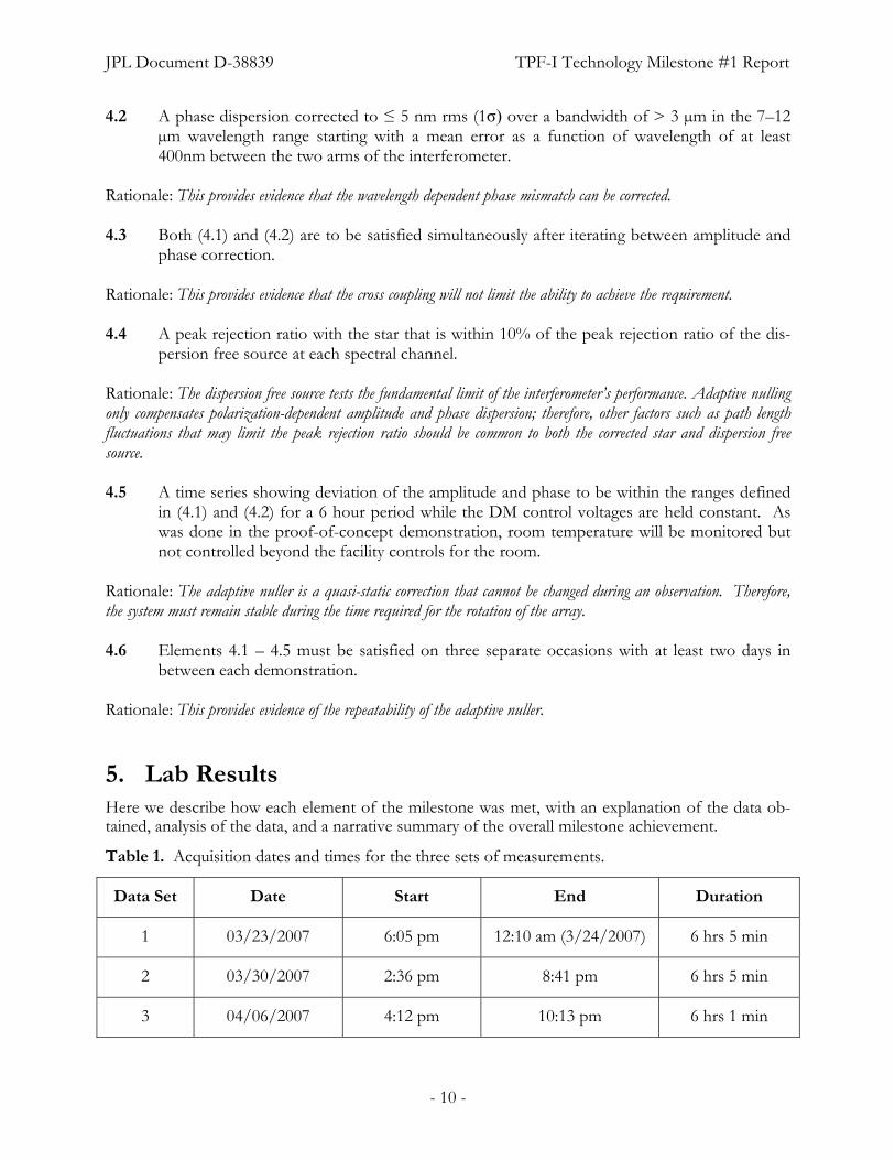
between each demonstration. Rationale: This provides evidence of the repeatability of the adaptive nuller. 5. Lab Results Here we describe how each element of the milestone was met, with an explanation of the data ob-tained, analysis of the data, and a narrative summary of the overall milestone achievement.

Table 1. Acquisition dates and times for the three sets of measurements.

Data Set Date Start End Duration

1 03/23/2007 6:05 pm 12:10 am (3/24/2007) 6 hrs 5 min

2 03/30/2007 2:36 pm 8:41 pm 6 hrs 5 min

3 04/06/2007 4:12 pm 10:13 pm 6 hrs 1 min


- 11 -

5.1. Data Acquisition

Requirement 4.5 (see Section 4.5) states the required duration of the tests. Requirement 4.6 (see Section 4.6) states the required time line over which the phase and intensity correction are to be measured. Table 1 indicates the times when data was taken and the total duration of each experi-ment. The duration of the tests and their time-line thus meets the requirements of 4.5 and 4.6. It is worth noting that the testbed was not used between the experiments described in this report.

5.2. Intensity correction

The intensity dispersion is measured by taking independent spectra of each arm of the interferome-ter. By adjusting an aperture in the reference arm, and the flat mirror at the focus of the parabola we can intentionally introduce an intensity mismatch with some spectral dependence.

Requirement 4.1 (see Section 4.1) is the success criteria for intensity correction. Figure 6a, 6b and 6c show the intensity imbalance between the arms of the spectrometer before and after correction. The initial intensity imbalance is set to be in excess of requirement 4.1 set forth in the Milestone Whitepaper of an error of 9% between the two arms. The corrected intensity is shown after the phase and intensity corrections converge. In all cases, the intensity correction was programmed to stop after it converged to less than 0.1% RMS difference between the two arms. This satisfies re-quirement 4.1 and 4.3 of the Milestone Whitepaper by demonstrating a capability to have a repeat-able correction to the intensity of <0.2% RMS difference.


- 12 -

8 9 10 11 120

2

4

6

8

10

Uncorrected Intensity Difference (9.2% RMS)

Unc

orre

cted

Inte

nsity

Diff

eren

ce (p

erce

nt)

Wavelength (um)

0.00

0.02

0.04

0.06

0.08

0.10

0.12

0.14

0.16

0.18

0.20

Corrected Intensity Difference (0.092% RMS)

Cor

rect

ed In

tens

ity D

iffer

ence

(Per

cent

)

b)

8 9 10 11 120

2

4

6

8

10


Unc

orre

cted

Inte

nsity

Diff

eren

ce (P

erce

nt)

Wavelength (um)

0.00

0.02

0.04

0.06

0.08

0.10

0.12

0.14

0.16

0.18

0.20


Cor

rect

ed In

tens

ity D

iffer

ence

(Per

cent

)

c)

8 9 10 11 120

2

4

6

8

10


Unc

orre

cted

Inte

nsity

Diff

eren

ce (p

erce

nt)

Wavelength (um)

0.00

0.02

0.04

0.06

0.08

0.10

0.12

0.14

0.16

0.18

0.20


Cor

rect

ed In

tens

ity D

iffer

ence

(per

cent

)

a)

8 9 10 11 120

2

4

6

8

10


Unc

orre

cted

Inte

nsity

Diff

eren

ce (p

erce

nt)

Wavelength (um)

0.00

0.02

0.04

0.06

0.08

0.10

0.12

0.14

0.16

0.18

0.20


Cor

rect

ed In

tens

ity D

iffer

ence

(Per

cent

)

b)

8 9 10 11 120

2

4

6

8

10


Unc

orre

cted

Inte

nsity

Diff

eren

ce (p

erce

nt)

Wavelength (um)

0.00

0.02

0.04

0.06

0.08

0.10

0.12

0.14

0.16

0.18

0.20


Cor

rect

ed In

tens

ity D

iffer

ence

(Per

cent

)

b)

8 9 10 11 120

2

4

6

8

10


Unc

orre

cted

Inte

nsity

Diff

eren

ce (P

erce

nt)

Wavelength (um)

0.00

0.02

0.04

0.06

0.08

0.10

0.12

0.14

0.16

0.18

0.20


Cor

rect

ed In

tens

ity D

iffer

ence

(Per

cent

)

c)

8 9 10 11 120

2

4

6

8

10


Unc

orre

cted

Inte

nsity

Diff

eren

ce (P

erce

nt)

Wavelength (um)

0.00

0.02

0.04

0.06

0.08

0.10

0.12

0.14

0.16

0.18

0.20


Cor

rect

ed In

tens

ity D

iffer

ence

(Per

cent

)

c)

8 9 10 11 120

2

4

6

8

10


Unc

orre

cted

Inte

nsity

Diff

eren

ce (p

erce

nt)

Wavelength (um)

0.00

0.02

0.04

0.06

0.08

0.10

0.12

0.14

0.16

0.18

0.20


Cor

rect

ed In

tens

ity D

iffer

ence

(per

cent

)

a)

8 9 10 11 120

2

4

6

8

10


Unc

orre

cted

Inte

nsity

Diff

eren

ce (p

erce

nt)

Wavelength (um)

0.00

0.02

0.04

0.06

0.08

0.10

0.12

0.14

0.16

0.18

0.20


Cor

rect

ed In

tens

ity D

iffer

ence

(per

cent

)

a)

Figure 6: Intensity measurements before and after correction for a) data set 1 b) data set 2 and c) data set 3.


- 13 -

5.3. Phase correction

The phase dispersion is measured from the spectral fringes obtained with the interferometer delay line set away from the null. The interferometer has an intentional mismatch of ZnSe glass between the two arms to provide dispersion for the adaptive nuller to correct.

Requirement 4.2 (see Section 4.2) is the success criteria for phase correction. Figure 7 shows the measured phase dispersion at the start of each data set. The uncorrected dispersion is measured with the mirror in the flat configuration. The corrected dispersion is shown after the intensity and phase corrections converge to within the requirements set forth in the Milestone Whitepaper.


- 14 -

8 9 10 11 12-1.0

-0.8

-0.6

-0.4

-0.2

0.0

0.2

0.4

0.6

0.8

1.0 Uncorrected Phase (406nm RMS)

Unc

orre

cted

Pha

se (u

m)

Wavelength (um)

-10

-8

-6

-4

-2

0

2

4

6

8

10

Corrected Phase (4.42nm RMS)

Cor

rect

ed P

hase

(nm

)

b)

8 9 10 11 12-1.0

-0.8

-0.6

-0.4

-0.2

0.0

0.2

0.4

0.6

0.8


Y A

xis

Title

Wavelength (um)

-10

-8

-6

-4

-2

0

2

4

6

8

10

Cor

rect

ed P

hase

(nm

)


c)

8 9 10 11 12-1.0

-0.8

-0.6

-0.4

-0.2

0.0

0.2

0.4

0.6

0.8


Unc

orre

cted

Pha

se (u

m)

Wavelength (um)

-10

-8

-6

-4

-2

0

2

4

6

8

10


Cor

rect

ed P

hase

(nm

)

a)

Unc

orre

cted

Pha

se (u

m)

8 9 10 11 12-1.0

-0.8

-0.6

-0.4

-0.2

0.0

0.2

0.4

0.6

0.8


Unc

orre

cted

Pha

se (u

m)

Wavelength (um)

-10

-8

-6

-4

-2

0

2

4

6

8

10


Cor

rect

ed P

hase

(nm

)

b)

8 9 10 11 12-1.0

-0.8

-0.6

-0.4

-0.2

0.0

0.2

0.4

0.6

0.8


Unc

orre

cted

Pha

se (u

m)

Wavelength (um)

-10

-8

-6

-4

-2

0

2

4

6

8

10


Cor

rect

ed P

hase

(nm

)

b)

8 9 10 11 12-1.0

-0.8

-0.6

-0.4

-0.2

0.0

0.2

0.4

0.6

0.8


Y A

xis

Title

Wavelength (um)

-10

-8

-6

-4

-2

0

2

4

6

8

10

Cor

rect

ed P

hase

(nm

)


c)

8 9 10 11 12-1.0

-0.8

-0.6

-0.4

-0.2

0.0

0.2

0.4

0.6

0.8


Y A

xis

Title

Wavelength (um)

-10

-8

-6

-4

-2

0

2

4

6

8

10

Cor

rect

ed P

hase

(nm

)


c)

8 9 10 11 12-1.0

-0.8

-0.6

-0.4

-0.2

0.0

0.2

0.4

0.6

0.8


Unc

orre

cted

Pha

se (u

m)

Wavelength (um)

-10

-8

-6

-4

-2

0

2

4

6

8

10


Cor

rect

ed P

hase

(nm

)

a)

8 9 10 11 12-1.0

-0.8

-0.6

-0.4

-0.2

0.0

0.2

0.4

0.6

0.8


Unc

orre

cted

Pha

se (u

m)

Wavelength (um)

-10

-8

-6

-4

-2

0

2

4

6

8

10


Cor

rect

ed P

hase

(nm

)

a)

Unc

orre

cted

Pha

se (u

m)

Figure 7: Phase measurements before and after correction for a) data set 1 b) data set 2 and c) data set 3.


- 15 -

The plots show a starting phase dispersion of at least 400nm RMS before correction, and the phase correction was programmed to stop after it converged to within 5nm RMS. This satisfies require-ment 4.2 and 4.3 of the Milestone Whitepaper by showing a repeatable simultaneous correction to the wavelength dependent mismatch of less than 5 nm RMS can be achieved.

5.4. Nulling test

The null of the interferometer is measured as outlined in section 3.2 of the Milestone Whitepaper. A null measurement is made with a CO2 laser operating at a wavelength of approximately 10 µm. Due to the single-frequency nature of the laser, this null should not be affected by dispersion, how-ever it will remain sensitive to other noise sources beyond the control of this testbed such as air fluc-tuations and vibration. The white light null is then measured without changing any settings on the interferometer.

Requirement 4.4 relates the demonstrated null-depth to the null-depth achieved with a dispersion free source. Figure 8 shows the difference between the null measured with the broad band light source, and with the laser. The uncorrected rejection ratios (inverse of the null) begin at less than 100:1 and are corrected by adjusting the phase and amplitude dispersion to achieve a rejection ratio close to 50,000:1. Although no particular nulling goal was defined in the Milestone Whitepaper, the difference between the laser and white light nulls for each test is less than 10%. The differences be-tween the laser and white light nulls are 7.3%, 8.4%, and 7.8% for data sets 1 through 3 respectively which satisfies requirement 4.4 set forth in the Milestone Whitepaper.

For these experiments we used a simple error budget model to predict nulling performance given the phase and amplitude correction. The model takes as input the current performance of the phase and amplitude correction, as well as other common factors which may limit null performance, such as optical path fluctuations and polarization effects. The model then computes the expected null depth, or, if given a null depth, the model can compute the amount of noise required from the vari-ous inputs that are consistent with the results. Given a 50,000:1 null and the performance of the phase and amplitude correction demonstrated in these experiments, and assuming no polarization effects, the model predicts about 13 nm of path length fluctuations. This level of residual uncor-rected dynamic path fluctuation is reasonably consistent with the control bandwidth and perform-ance of the delay line servos.


- 16 -

8 9 10 11 121E-6

1E-5

1E-4

1E-3

0.01

Corrected Null (46000:1) Uncorrected Null (60:1) Laser Null (49600:1) Detector Noise

Rej

ectio

n R

atio

(nul

l/pea

k)

Wavelength (um)

a)

8 9 10 11 121E-6

1E-5

1E-4

1E-3

0.01

0.1

1


Rej

ectio

n R

atio

(nul

l/pea

k)

Wavelength (um)

b)

c)

8 9 10 11 121E-6

1E-5

1E-4

1E-3

0.01

0.1

1 Corrected Null (45800:1) Uncorrected Null (54:1) Laser Null (49700:1) Detector Noise

Rej

ectio

n R

atio

(nul

l/pea

k)

Wavelength (um)

8 9 10 11 121E-6

1E-5

1E-4

1E-3

0.01


Rej

ectio

n R

atio

(nul

l/pea

k)

Wavelength (um)

a)

8 9 10 11 121E-6

1E-5

1E-4

1E-3

0.01


Rej

ectio

n R

atio

(nul

l/pea

k)

Wavelength (um)

a)

8 9 10 11 121E-6

1E-5

1E-4

1E-3

0.01

0.1

1


Rej

ectio

n R

atio

(nul

l/pea

k)

Wavelength (um)

b)

8 9 10 11 121E-6

1E-5

1E-4

1E-3

0.01

0.1

1


Rej

ectio

n R

atio

(nul

l/pea

k)

Wavelength (um)

b)

c)

8 9 10 11 121E-6

1E-5

1E-4

1E-3

0.01

0.1


Rej

ectio

n R

atio

(nul

l/pea

k)

Wavelength (um)

c)

8 9 10 11 121E-6

1E-5

1E-4

1E-3

0.01

0.1


Rej

ectio

n R

atio

(nul

l/pea

k)

Wavelength (um)

Figure 8: Nulling comparison for a) data set 1, b) data set 2, and c) data set 3.


- 17 -

5.5. Stability

Once the correction is set by the adaptive nuller, it must remain stable during an observation for TPF-I. Requirement 4.5 of the Milestone Whitepaper states after the initial correction is made the phase and amplitude correction will remain within the bounds defined for at least 6 hours. We show here that this requirement has been met.

Figure 9 is a plot of the RMS phase measured across the 8–12 µm band as a function of time. In the first data set there is a drift initially from the correction, however, the level stays below the 5-nm re-quirement. The second set was taken much earlier in the day than the other two, and hence the there may have been more building vibration affecting the testbed.

Figure 10 shows the RMS of the percent amplitude difference measured across the band as a func-tion of time. The percent amplitude difference stays well below the requirement of 0.2% during the six-hour test.

Finally, Fig. 11 shows the rejection ratio as a function of time. Since the null measurement inter-rupts the phase and intensity measurement, the null was measured after every eight phase and inten-sity measurements. The nulls are stable around 2.2 × 10-5 or 45,000:1. The lack of a trend following the phase or amplitude plots in Figs. 9 and 10 indicates that dispersion is not the limiting factor for the null depth being measured. In theory if the phase dispersion of 5nm RMS and intensity disper-sion of 0.1% RMS were the only effects limiting the null then we should be able to achieve rejection ratio better than 350,000:1. The most likely source for the limitation of the null depth is residual path length fluctuations. These may be uncorrected residuals, perhaps induced by the metrology system.


- 18 -

0 1 2 3 4 5 6 73.8

4.0

4.2

4.4

4.6

4.8

5.0

RM

S P

hase

(nm

)

Time (Hours)

0 1 2 3 4 5 6 73.8

4.0

4.2

4.4

4.6

4.8

5.0

RM

S P

hase

(nm

)

Time (Hours)

0 1 2 3 4 5 6 73.8

4.0

4.2

4.4

4.6

4.8

5.0

RM

S P

hase

(nm

)

Time (Hours)

a)

b)

c)

0 1 2 3 4 5 6 73.8

4.0

4.2

4.4

4.6

4.8

5.0

RM

S P

hase

(nm

)

Time (Hours)

0 1 2 3 4 5 6 73.8

4.0

4.2

4.4

4.6

4.8

5.0

RM

S P

hase

(nm

)

Time (Hours)

0 1 2 3 4 5 6 73.8

4.0

4.2

4.4

4.6

4.8

5.0

RM

S P

hase

(nm

)

Time (Hours)

a)

b)

c)

Figure 9: RMS phase as a function of time for a) data set 1, b) data set 2, and c) data set 3


- 19 -

0 1 2 3 4 5 6 70.05

0.06

0.07

0.08

0.09

0.10

0.11

0.12

Per

cent

Inte

nsity

Diff

eren

ce (R

MS

)

Time (Hours)

a)

0 1 2 3 4 5 6 70.05

0.06

0.07

0.08

0.09

0.10

0.11

0.12

Per

cent

Inte

nsity

Diff

eren

ce (R

MS

)

Time (Hours)

b)

0 1 2 3 4 5 6 70.05

0.06

0.07

0.08

0.09

0.10

0.11

0.12

Per

cent

Inte

nsity

Diff

eren

ce (R

MS

)

Time (Hours)

c)

0 1 2 3 4 5 6 70.05

0.06

0.07

0.08

0.09

0.10

0.11

0.12

Per

cent

Inte

nsity

Diff

eren

ce (R

MS

)

Time (Hours)

a)

0 1 2 3 4 5 6 70.05

0.06

0.07

0.08

0.09

0.10

0.11

0.12

Per

cent

Inte

nsity

Diff

eren

ce (R

MS

)

Time (Hours)

a)

0 1 2 3 4 5 6 70.05

0.06

0.07

0.08

0.09

0.10

0.11

0.12

Per

cent

Inte

nsity

Diff

eren

ce (R

MS

)

Time (Hours)

b)

0 1 2 3 4 5 6 70.05

0.06

0.07

0.08

0.09

0.10

0.11

0.12

Per

cent

Inte

nsity

Diff

eren

ce (R

MS

)

Time (Hours)

b)

0 1 2 3 4 5 6 70.05

0.06

0.07

0.08

0.09

0.10

0.11

0.12

Per

cent

Inte

nsity

Diff

eren

ce (R

MS

)

Time (Hours)

c)

0 1 2 3 4 5 6 70.05

0.06

0.07

0.08

0.09

0.10

0.11

0.12

Per

cent

Inte

nsity

Diff

eren

ce (R

MS

)

Time (Hours)

c)

Figure 10: RMS amplitude stability as a function of time for a) data set 1, b) data set 2, and c) data set 3.


- 20 -

a)

0 1 2 3 4 5 61.8x10-5

2.0x10-5

2.2x10-5

2.4x10-5

2.6x10-5

2.8x10-5

Rej

ectio

n ra

tio (n

ull/p

eak)

Time (Hours)b)

0 1 2 3 4 5 61.8x10-5

2.0x10-5

2.2x10-5

2.4x10-5

2.6x10-5

2.8x10-5

Rej

ectio

n R

atio

(nul

l/pea

k)

Time (Hours)

c)

0 1 2 3 4 5 61.8x10-5

2.0x10-5

2.2x10-5

2.4x10-5

2.6x10-5

2.8x10-5

Rej

ectio

n R

atio

(nul

l/pea

k)

Time (Hours)

a)

0 1 2 3 4 5 61.8x10-5

2.0x10-5

2.2x10-5

2.4x10-5

2.6x10-5

2.8x10-5

Rej

ectio

n ra

tio (n

ull/p

eak)

Time (Hours)

a)

0 1 2 3 4 5 61.8x10-5

2.0x10-5

2.2x10-5

2.4x10-5

2.6x10-5

2.8x10-5

Rej

ectio

n ra

tio (n

ull/p

eak)

Time (Hours)b)

0 1 2 3 4 5 61.8x10-5

2.0x10-5

2.2x10-5

2.4x10-5

2.6x10-5

2.8x10-5

Rej

ectio

n R

atio

(nul

l/pea

k)

Time (Hours)

b)

0 1 2 3 4 5 61.8x10-5

2.0x10-5

2.2x10-5

2.4x10-5

2.6x10-5

2.8x10-5

Rej

ectio

n R

atio

(nul

l/pea

k)

Time (Hours)

c)

0 1 2 3 4 5 61.8x10-5

2.0x10-5

2.2x10-5

2.4x10-5

2.6x10-5

2.8x10-5

Rej

ectio

n R

atio

(nul

l/pea

k)

Time (Hours)

c)

0 1 2 3 4 5 61.8x10-5

2.0x10-5

2.2x10-5

2.4x10-5

2.6x10-5

2.8x10-5

Rej

ectio

n R

atio

(nul

l/pea

k)

Time (Hours)

Figure 11: Measured null as a function of time for a) data set 1, b) data set 2, and c) data set 3.


- 21 -

5.6. Throughput

The throughput measurement was done with the CO2 laser at full power for the light source and with a thermopile power meter as the sensor. With the power meter directly in front of the first op-tic in adaptive nuller compensator, we measured a power of 4mW. With the power meter after the last optic in the adaptive nuller compensator we measured a power that would fluctuate between 3mW and 4mW. Unfortunately, the resolution of the sensor is limited to 1mW, so this measurement sets a maximum insertion loss for the compensator at 25%. 6. Conclusions This report has described the Adaptive Nulling Testbed concept and layout, the data collected and the results.

We conclude that the TPF-I Technology Milestone #1 has been demonstrated. We have restated the success criteria and shown, step by step, that the requirements have been met. We have shown that the amplitude and phase dispersion can be corrected using adaptive nulling. We have demon-strated that the testbed can be stable for at least six hours, and that the tests are repeatable. We have shown that we can achieve nulls close to that of the dispersion free source. In summary, all tests performed were within the requirements set forth for this milestone.

terrestrial planet finder interferometer tpf-i · pdf filejpl document d-38839 terrestrial...

Documents