testimony of david b. south retired emeritus … · retired emeritus professor, auburn university...
TRANSCRIPT

Testimony of David B South
Retired Emeritus Professor Auburn University
Subcommittee on Green Jobs and the New Economy
3 June 2014
Human Activity more so than Climate Change Affects the Number and Size of Wildfires
I am David B South Emeritus Professor of Forestry Auburn University In 1999 I was awarded
the Society of American Forestersrsquo Barrington Moore Award for research in the area of
biological science and the following year I was selected as Auburn Universityrsquos ldquoDistinguished
Graduate Lecturerrdquo In 1993 I received a Fulbright award to conduct tree seedling research at the
University of Stellenbosch in South Africa and in 2002 I was a Canterbury Fellow at the
University of Canterbury in New Zealand My international travels have allowed me the
opportunity to plant trees on six continents
It is a privilege for me to provide some data and views on factors that affect forests and wildfires
Foresters know there are many examples of where human activity affects both the total number
and size of wildfires Policy makers who halt active forest management and kill ldquogreenrdquo
harvesting jobs in favor of a ldquohands-offrdquo approach contribute to the buildup of fuels in the forest
This eventually increases the risk of catastrophic wildfires To attribute this human-caused
increase in fire risk to carbon dioxide emissions is simply unscientific However in todayrsquos
world of climate alarmism where accuracy doesnrsquot matter I am not at all surprised to see many
journalists spreading the idea that carbon emissions cause large wildfires
There is a well-known poem called the ldquoSerenity prayerrdquo It states ldquoGod grant me the serenity
to accept the things I cannot change the courage to change the things I can and wisdom to know
the differencerdquo Now that I am 63 I realize I canrsquot change the behavior of the media and I canrsquot
change the weather Early in my career I gave up trying to get the media to correct mistakes
about forest management and to avoid exaggerations I now concentrate on trying to get my
colleagues to do a better job of sticking to facts I leave guesses about the future to others
Untrue claims about the underlying cause of wildfires can spread like ldquowildfirerdquo For example
the false idea that ldquoWildfires in 2012 burned a record 92 million acres in the USrdquo is cited in
numerous articles and is found on more than 2000 web sites across the internet In truth many
foresters know that in 1930 wildfires burned more than 4 times that amount Wildfire in 2012
was certainly an issue of concern but did those who push an agenda really need to make
exaggerated claims to fool the public
Here is a graph showing a decreasing trend in wildfires from 1930 to 1970 and an increasing
trend in global carbon emissions If we ldquocherry pickrdquo data from 1926 to 1970 we get a negative
relationship between area burned and carbon dioxide However if we ldquocherry pickrdquo data from
1985 to 2013 we get a positive relationship Neither relationship proves anything about the
effects of carbon dioxide on wildfires since during dry seasons human activity is the
overwhelming factor that determines both the number and size of wildfires
Figure 1
In the lower 48 states there have been about ten ldquoextreme megafiresrdquo which I define as burning
more than 1 million acres Eight of these occurred during cooler than average decades These
data suggest that extremely large megafires were 4-times more common before 1940 (back when
carbon dioxide concentrations were lower than 310 ppmv) What these graphs suggest is that we
cannot reasonably say that anthropogenic global warming causes extremely large wildfires
Figure 2
Seven years ago this Committee conducted a hearing about ldquoExamining climate change and the
mediardquo [Senate Hearing 109-1077] During that hearing concern was expressed over the
weather which was mentioned 17 times hurricanes which were mentioned 13 times and
droughts which were mentioned 4 times In the 41000 word text of that hearing wildfires (that
occur every year) were not mentioned at all I am pleased to discuss forestry practices because
unlike hurricanes droughts and the polar vortex we can actually promote forestry practices that
will reduce the risk of wildfires Unfortunately some of our national forest management policies
have in my view contributed to increasing the risk of catastrophic wildfires
In conclusion I am certain that attempts to legislate a change in the concentration of carbon
dioxide in the atmosphere will have no effect on reducing the size of wildfires or the frequency
of droughts In contrast allowing active forest management to create economically-lasting
forestry jobs in the private sector might reduce the fuel load of dense forests In years when
demand for renewable resources is high increasing the number of thinning and harvesting jobs
might have a real impact in reducing wildfires
Thank you for this opportunity to address the Subcommittee
Additional thoughts and data
A list of names and locations of 13 megafires in North America
Year Fire Name Location Lives lost Acres burned
1825 Miramichi New Brunswick- Maine gt 160 3 million
1845 Great Fire Oregon - 15 million
1868 Silverton Oregon - 1 million
1871 Peshtigo Wisconsin-Michigan gt1500 378 million
1881 Thumb Michigan gt280 gt24 million
1889 Feb-15-16 South Carolina 14 3 million
1902 Yacoult Washington and Oregon - gt 1 million
1910 Big Blowup Idaho Montana 85 gt3 million
1918 Cloquet-Moose
Lake
Minnesota 450 12 million
1950 Chinchaga British Columbia
Alberta
- 35 million
1988 Yellowstone Montana Idaho - 158 million
2004 Taylor Complex Alaska - 13 million
2008 Lightning series California 23 gt15 million
Figure 3 is another timeline that was constructed by examining fire scars on trees from the
Southwest (Swetnam and Baisan 1996) Fire suppressionprevention activities started having an
effect at the end of the 19th
century and this apparently reduced the wide-scale occurrence of
wildfires in the Southwest Both of these graphs show a decline in megafires after 1920 This
tells me that humans affect both the size and cycle of wildfires to a much greater extent than does
increasing levels of carbon dioxide in the atmosphere
Figure 3
++++++++++++++++++++++++++++++++
The ldquomost destructive firerdquo in history
I must comment on the term ldquomost destructiverdquo when used in the context of wildfires When I
ask what ldquomost destructiverdquo actually means I get several answers In some articles the number
used (when there actually is a number) is calculated using nominal dollar amounts Therefore
the rate of inflation is one factor (possibly the deciding factor) that causes fires to become more
ldquodestructiverdquo over time In other cases the ranking just involves counting the number of
structures burned This takes inflation out of the equation but it inserts urban sprawl into the
equation For example ldquothe number of housing units within half a mile of a national forest grew
from 484000 in 1940 to 18 million in 2000rdquo Therefore the increasing wealth of our nation
(more building in fire-prone areas) can easily explain why wildfires have become ldquomore
destructiverdquo over time These facts are rarely mentioned by journalists who use the ldquomost
destructiverdquo term when attributing the damage to ldquoclimate changerdquo Scientifically I say the term
ldquomost destructiverdquo holds little meaning For example was the 1871 fire that killed over 1500
people (possibly 2400) and burned over 375 million acres the ldquomost destructiverdquo in US history
If not why not
+++++++++++++++++++++++++++++++
High fuel load = high wildfire danger
Fuel loading (or fuel volume) is reported as the amount of fuel available per acre The higher the
fuel loading the more heat produced during a wildfire Intense wildfires occur during dry
seasons when winds are high and there is high fuel loading The classification of fuels includes
(1) surface (2) ladder and (3) crown fuels The risk of wildfires since 1977 has increased on
federal lands in part because of an increase in the ldquofuel loadrdquo This increase is due to tree
growth plus a reduction in harvesting logs for wood products (see Figure 6) The evidence in the
figure below indicates that as fuel loads on timberland increase the area of wildfire increases
Figure 4
The theory that higher fuel loads cause an increase in wildfires (during dry seasons) is also
supported by data from California In just a decade fuel loads increased on timber land by 16
percent while average wildfire size increased by 32 percent
Figure 5
In cases where policy allows foresters can reduce the risk of destructive wildfires by reducing
fuel loads They can reduce ladder and crown fuels by harvesting trees and transporting the logs
to a mill This can be accomplished as final harvests economic thinnings firebreak thinnings
and biomass thinnings (eg to make pellets) Surface fuels can be reduced by conducting
prescribed burns (aka controlled burns) However in the past policy has been determined by
concerns expressed by journalists and activists who are against the cutting of trees Many
ldquopreserve the forestrdquo and ldquoanti-forest managementrdquo policies end up increasing the risk of intense
wildfires For example a number of climate experts recently (24 April 2014) signed a letter
hoping to reduce the number of ldquogreen jobsrdquo in North Carolina These experts are apparently
against the cutting of trees to produce wood pellets for export to the UK They say that ldquoa
growing body of evidence suggests that trees rather than wood waste are the primary source of
the wood pellets exported to the UK from the Southern USrdquo
+++++++++++++++++++++++++++++++
Would a return to harvesting 12 billion board feet per year reduce fuel loads on National
Forests
From about 1965 to 1990 the US Forest Service harvested about 12 billion board feet per year
on National Forests Removing this wood reduced the rate of increase in fuel loads on our
National Forests As a result the wood volume on timber land in the West changed very little
between 1977 (3467 billion cubic feet) and 1987 (347 billion cubic feet) In contrast wood
volume over the next 10-years increased by 5 percent Obviously stopping the harvesting of
trees has increased wildfire risk in National Forests (due to increasing average wood biomass and
fuel loads)
Figure 6
+++++++++++++++++++++++++++++++
Correlation does not prove causation
I assume most Senators (and even some journalists) know that finding a ldquosignificantrdquo trend does
not prove causation (httpwwwlatimescombusinesshiltzikla-fi-mh-see-correlation-is-not-
causation-20140512-columnhtml) In fact a low occurrence of large megafires over the past 90
years does not prove that droughts were more common before 1950 Actual weather records or
analysis of tree-rings can be used to document drought events
Those committed to the scientific process know that the cause behind the decline in megafires is
not proved by a simple correlation Although Figure 2 (above) indicates large megafires were
more common in decades with cooler temperatures this is certainly not proof of a relationship
with temperature In reality human activity (eg effective fire suppression) is the real causation
for a decline in million-acre wildfires
Figure 7 is a graph of a short-term (ie 28 year) trend for wildfire size in the USA When using
data from 1985 to 2013 the trend suggests the total area burned increased by 19 million acres
per decade This type of correlation has been the driving force behind the current media frenzy
Figure 7
Regarding a trend line similar to that in Figure 7 here is what one journalist wrote ldquoUS wildfires
have gotten much bigger over the past three decades Theres some variation from year to year
but the overall trend is upward One recent study in Geophysical Research Letters found that
wildfires in the western United States grew at a rate of 90000 acres per year between 1984 and
2011 Whats more the authors found the increase was statistically unlikely to be due to random
chancerdquo
In contrast Figure 1 illustrates that for the lower 48 states the amount of wildfires declined at a
rate of 400000 acres per year between 1926 and 2013 This decline was also statistically
ldquounlikely to be due to random chancerdquo (ie 1 chance out of 10000) [Note The rate of decline
from 1926 to 1956 was about 13 million acres per year] I have never seen the print media
publish a graph like Figure 1 even though similar ones are easy to find on the internet
(httpwwwfaoorgdocrep010ai412eai412e09jpg) They are either reluctant to inform the
public about the history of wildfires or they simply donrsquot know the information is available
Either way they might not realize a ldquostatistically significantrdquo relationship reported in their article
does not mean the relationship has any real meaning
Figure 8
Here is an example of how the wrong conclusion can be made even with a ldquosignificant
correlationrdquo Letrsquos assume that people cause wildfires and that more people cause more
wildfires We know that people cause carbon emissions and more people cause more carbon
emissions (Figure 8) Journalists might assume that carbon emissions are causing more wildfires
(due to a significant trend) but the driving force behind more wildfires is likely due to people
causing more wildfires Good scientists point out to the public all the various factors that might
explain an increase in wildfires In contrast those with an agenda will tell the public only about
the factors that support their agenda (or beliefs) They ignore scientists who warn readers that
ldquoDue to complex interacting influences on fire regimes across the western US and the relatively
short period analyzed by this study care must be exercised in directly attributing increases in fire
activity to anthropogenic climate changerdquo
+++++++++++++++++++++++++++++++
In reality people affect both the size and number of wildfires
Unlike hurricanes droughts and tornadoes humans cause many wildfires During the 19th
century Native Americans and European immigrants increased the number of wildfires The
following graph suggests the fires in the Boston Mountains of Arkansas were related to the
population of Cherokee Indians (Guyette Spetich and Stambaugh 2006)
Figure 9
In most places in the US humans are the major cause of wildfires In 2012 only about 5 percent
of fires in California were caused by lightning The Rim Fire (100 miles east of San Francisco)
was ignited by a campfire in 2013 and was perhaps the third largest fire in California Even so
some (who might be against cutting of trees to lower fuel levels) contend severe fire seasons are
the result of prolonged drought combined with lightning If this human-caused wildfire had not
occurred the amount of wildfires in California that year would have been reduced by 44
Since one human fire can increase acres burned by over 250000 acres I say it is unscientific to
attribute trends in wildfires to carbon dioxide levels without accounting for the various ways
humans actually affect wildfires (eg arson smoking target practice accidents etc)
Figure 10
Figure 11
In areas that are unpopulated fire fighters can concentrate their limited resources on suppressing
the fire However in areas where population growth has increased the density of houses some
crews are diverted to protecting property instead of attacking the fire As a result the relative
size of the fire increases The policy of allowing more homes to be built in fire-prone areas
likely has increase the size of future fires (if more resources are devoted to protecting the
homes) Randy Eardley (a spokesperson for the Bureau of Land Management) said that in the
past ldquoit was rare that you would have to deal with fire and structuresrdquo ldquoNowadays itrsquos the
opposite Itrsquos rare to have a fire that doesnrsquot involve structuresrdquo In fact I was recently told that
one of the primary reasons for increased burned acres is that - in the interest of firefighter safety
cost and biotic benefits ldquofire officers are more willing to back offrdquo and let the wildfire burn out
+++++++++++++++++++++++++++++++
Some forests receive more rainfall now than 100 years ago
Examining historical weather data shows that some forests now receive more rainfall on average
than occurred a century ago For example precipitation in the Northeast has increased about
10 Of course rainfall pattern is very important in the cycle of droughts but one advantage of
an increase in rainfall might be an increase in growth of trees The following are trends in
precipitation for various regions in the lower 48 states Northeast +41rdquo per century Upper
Midwest +28rdquo South +25rdquo Southeast +06rdquo Southwest -02rdquo West no change Northern
Rockies and Plains +05rdquo Northwest +07rdquo
Figure 12
In some places the extra rainfall might have resulted in a reduction in wildfires For example
summer precipitation in British Columbia increased from 1920 to 2000 In one region the
increase may have been over 45 Authors of the study (Meyn et al 2013) observed a
ldquosignificant decrease in province-wide area burnedrdquo and they said this decrease was ldquostrongly
related to increasing precipitation more so than to changing temperature or drought severityrdquo In
some areas a benefit of an increase in precipitation could be fewer wildfires
+++++++++++++++++++++++++++++++
Some forests receive less rainfall now than 40 years ago
Drought increases the risk of wildfire The extent of wildfires for any given year will depend on
if a drought occurs that year One should expect some variability in the occurrence of droughts
and we can document various drought cycles by using the NOAA web site ldquoClimate at a
Glancerdquo We might also expect a single large wildfire to burn more acres in a drought year than
in a rainy year Therefore it is not surprising that total area burned is higher in drought years
than in non-drought years
As previously mentioned some journalists are spreading the idea that carbon dioxide is causing
more droughts But if it were true we should see droughts increasing globally (not just in one
drought-prone region of the US) The following figure illustrates the global pattern of drought
since 1982 and it clearly suggests that droughts globally have not gotten worse over the two
decade timeframe (Hao et al 2014) It appears that some journalists are not aware of this
global pattern Of course some might be aware of this pattern but it does not fit their narrative
As a result they report that droughts for a specific location increased during a decade
Figure 13
+++++++++++++++++++++++++++++++
Risk of pine beetles increase on forests with no thinning
Pine beetles have killed millions of trees in Canada and in the United States Foresters and
entomologists know that pine beetle outbreaks are cyclical in nature When pine trees are under
stress they attract pine beetles Trees undergo stress when they are too close together (ie too
dense) and things get worse when there is a drought Once conditions are right the beetles thrive
in stressed trees and the progeny attack more trees and the domino effect begins Foresters and
ecologists know that pine beetle cycles have occurred naturally over thousands of years
Figure 14
One factor that increases the risk of a beetle outbreak are policies that do not permit the thinning
of trees State and national forestry organizations know the risk of a beetle outbreak is higher in
counties occupied by National Forests For example in Texas the US Forest Service says that
ldquoVery little suppression took place during the last outbreak A majority of those treatments were
designed to protect RCW habitat as mandated by the Endangered Species act SPB were left
alone in most of the wilderness and killed large acreagesrdquo In contrast some ldquoenvironmentalrdquo
groups object to beetle suppression methods that involve cutting trees in wilderness areas As a
result thinning operations are delayed beetle attack stressed trees and then large populations of
beetles spread to adjacent privately-owned forests After the trees die the risk of wildfire
increases Wildfires start (due to carelessness or accidents or arson) and large expenditures are
made to put the fire out Journalists then report that carbon dioxide caused the inferno The
public concern over wildfires might cause some in Washington to want to increase the cost of
energy For example this month my electrical cooperative sent me an e-mail suggesting that
new EPA regulations could increase my bill by 50 Of course we know that increasing the cost
of energy will hurt the poor more than the wealthy
Figure 15
Foresters tell the public that the best way to prevent a beetle outbreak is to thin the forest to will
increase tree health We also know that planting too many seedlings per acre will also increase
the risk of beetles
httpwwwforestrystatealusPublicationsTREASURED_Forest_Magazine200520Summer
How20to20Grow20Beetle20Bait20-20Revisitedpdfly-owned forests
In contrast the public also tells foresters how to manage beetle risks in wilderness areas The
following is just two pages of a seven-page document illustrating how much time and man-hours
are wasted before operations to reduce the risk of pine beetles can precede in wilderness areas
+++++++++++++++++++++++++++++++
Dr South offers a bet on sea level rise for year 2024
In the past I have had the good fortune to make a few bets with professors
(httpwwwaaesauburneducommpubshighlightsonlinesummer99southhtml) For example
I won a bet on the future price of oil and was successful in betting against Dr Julian Simon on
the price of sawtimber (ie he sent me a check a year after making the bet) Five years ago I
offered to bet on an ldquoice freerdquo Arctic by the summer of 2013 but a BBC journalist [who wrote a
2007 article entitled ldquoArctic summers ice-free lsquoby 2013rsquo rdquo] and several ice experts declined my
offer To date the number of bets I have made has been limited since I have a hard time finding
individuals who are confident enough to make a wager on their predictions
I would like to take this opportunity to offer another ldquoglobal warmingrdquo bet This time the
outcome will be based on sea level data for Charleston SC Recently I was told that ldquoIf we do
nothing to stop climate change scientific models project that there is a real possibility of sea
level increasing by as much as 4 feet by the end of this centuryrdquo
At Charleston the rate of increase in sea level has been about 315 mm per year A four foot
increase (over the next 86 years) could be achieved by rate of 14 mm per year I am willing to
bet $1000 that the mean value (eg the 310 number for year 2012 in Figure 16) will not be
greater than 70 mmyr for the year 2024 I wonder is anyone really convinced the sea will rise
by four feet and if so will they take me up on my offer Dr Julian Simon said making bets was
a good way to see who was serious about their beliefs and who is just ldquotalking the talkrdquo
Figure 16
Annual change in sea level at Charleston SC
Figure 17
httptidesandcurrentsnoaagovsltrendssltrends_stationshtmlstnid=8665530
Selected References
Arno SF 1980 Forest fire history in the northern Rockies Journal of Forestry 78460-465
Botts H Jeffery T Kolk S McCabe S Stueck B Suhr L 2013 Wildfire hazard risk Report
Residential Wildfire Exposure Estimates for the Western United States CoreLogic Inc httpwwwcorelogiccomabout-usresearchtrendswildfire-hazard-risk-reportaspx
Dennison PE Brewer SC Arnold JD Moritz MA 2014 Large wildfire trends in the
western United States 1984ndash2011 Geophysical Research Letters
Guyette RP Spetich MA Stambaugh MC 2006 Historic fire regime dynamics and forcing
factors in the Boston Mountains Arkansas USA Forest Ecol Manage 234293ndash304
Hao Z AghaKouchak A Nakhjiri N Farahmand A 2014 Global integrated drought
monitoring and prediction system Scientific Data 1 Article number 140001
Layser EF 1980 Forestry and climatic change Journal of Forestry 78678-682
Meyn A Schmidtlein S Taylor SW Girardin MP Thonicke K Cramer W 2013
Precipitation-driven decrease in wildfires in British Columbia Regional Environmental
Change 13(1) 165-177
Stein SM Menakis J Carr MA Comas SJ Stewart SI Cleveland H Bramwell L Radeloff
VC 2013 Wildfire wildlands and people understanding and preparing for wildfire in the
wildland-urban interfacemdasha Forests on the Edge report Gen Tech Rep RMRS-GTR-299 Fort
Collins CO US Department of Agriculture Forest Service Rocky Mountain Research Station
36 p
Stephens SL Mclver JD Boerner REJ Fettig CJ Fontaine JB Hartsough BR Kennedy PL
Dylan WS 2012 Effects of forest fuel-reduction treatments in the United States Bioscience
63549-560
Swetnam T Baisan C 1996 Historical fire regime patterns in the southwestern United States
since AD 1700 In CD Allen (ed) Fire Effects in Southwestern Fortest Proceedings of the 2nd
La Mesa Fire Symposium pp 11-32 USDA Forest Service Rocky Mountain Research Station
General Technical Report RM-GTR-286
LETTERS
What If Our GuessesAre Wrong
This old professor would like to com-ment on four ldquoclimate changerdquo articles A1973 article entitled ldquoBrace yourself foranother ice agerdquo (Science Digest 5757ndash61)contained the following quote ldquoMan isdoing these thingshellip such as industrial pol-lution and deforestation that have effects onthe environmentrdquo A 1975 article aboutldquoWeather and world foodrdquo (Bulletin of theAmerican Meteorological Society 561078ndash1083) indicated the return of an ice agewould decrease food production The au-thor said ldquothere is an urgent need for a bet-ter understanding and utilization of infor-mation on weather variability and climatechangehelliprdquo Soon afterwards Earle Layserwrote a paper about ldquoForests and climaterdquo(Journal of Forestry 78678ndash682) The fol-lowing is an excerpt from his 1980 paperldquoOne degree [F] may hardly seem signifi-cant but this small change has reduced thegrowing season in middle latitudes by twoweeks created severe ice conditions in theArctic caused midsummer frosts to returnto the upper midwestern United States al-tered rainfall patterns and in the winter of1971ndash1972 suddenly increased the snowand ice cover of the northern hemisphere byabout 13 percent to levels where it has sinceremainedrdquo (Bryson 1974) Spurr (1953) at-tributed significant changes in the forestcomposition in New England to mean tem-perature changes of as little as 2 degreesGenerally the immediate effects of climaticchange are the most striking near the edge ofthe Arctic (Sutcliffe 1969 p 167) wheresuch things as the period of time ports areice-free are readily apparent However otherexamples cited in this article show that sub-tle but important effects occur over broadareas particularly in ecotonal situations suchas the northern and southern limits of theboreal forest or along the periphery of a spe-ciesrsquo range
Among these papers Layserrsquos paper hasbeen cited more often ( 20 times) but forsome reason it has been ignored by several
authors (eg it has not been cited in anyJournal of Forestry papers) Perhaps it is for-tunate that extension personnel did notchoose to believe the guesses about a comingice age If they had chosen this ldquoopportunityfor outreachrdquo landowners might have beenadvised to plant locally adapted genotypesfurther South (to lessen the impendingthreat to healthy forests) Since the coolingtrend ended such a recommendation wouldhave likely reduced economic returns for thelandowner
A fourth article was about ldquostate serviceforestersrsquo attitudes toward using climate andweather informationrdquo (Journal of Forestry1129ndash14) The authors refer to guessesabout the future as ldquoclimate informationrdquoand in just a few cases they confuse thereader by mixing the terms ldquoclimaterdquo andldquoweatherrdquo For example a forecast that nextwinter will be colder than the 30-year aver-age is not an example of a ldquoseasonal climateforecastrdquo Such a guess is actually a ldquoweatherforecastrdquo (like the ones available from wwwalmanaccomweatherlongrange) Every-one should know that the World Meteoro-logical Organization defines a ldquoclimate nor-malrdquo as an average of 30 years of weather data(eg 1961ndash1990) A 3-month or 10-yearguess about future rainfall patterns is tooshort a period to qualify as a ldquofuture climateconditionrdquo Therefore young foresters (50years old) are not able to answer the questionldquohave you noticed a change in the climaterdquosince they have only experienced one climatecycle They can answer the question ldquohaveyou noticed a change in the weather overyour lifetimerdquo However 70-year-olds cananswer the question since they can comparetwo 30-year periods (assuming they stillhave a good memory)
Flawed computer models have overesti-mated (1) the moonrsquos average temperature(2) the rate of global warming since the turnof the century (3) the rate of melting of Arc-tic sea ice (4) the number of major Atlantichurricanes for 2013 (5) the average Febru-ary 2014 temperature in Wisconsin (136degC) etc Therefore some state service forest-ers may be skeptical of modelers who predict
an increase in trapped heat and then a fewyears later attempt to explain away theldquomissing heatrdquo Overestimations might ex-plain why only 34 out of 69 surveyed forest-ers said they were interested in ldquolong-rangeclimate outlooksrdquo Some of us retired forest-ers remember that cooling predictions madeduring the 1970s were wrong Even ldquointer-mediate-termrdquo forecasts for atmosphericmethane (made a few years ago with the aidof superfast computers) were wrong There-fore I am willing to bet money that theldquolong-range outlooks of climate suitabilityrdquofor red oak will not decline by the amountpredicted (ie tinyurlcomkykschq) I dowonder why 37 foresters (out of 69 sur-veyed) would desire such guesses if outreachprofessionals are not willing to bet money onthese predictions
I know several dedicated outreach per-sonnel who strive to provide the public withfacts regarding silviculture (eg on mostsites loblolly pine seedlings should be plantedin a deep hole with the root collar 13ndash15 cmbelowground) However if ldquoright-thinkingrdquooutreach personnel try to convince land-owners to alter their forest managementbased on flawed climate models then I fearpublic support for forestry extension mightdecline I wonder will the public trust us ifwe donrsquot know the difference between ldquocli-materdquo and ldquoweatherrdquo wonrsquot distinguish be-tween facts and guesses and wonrsquot betmoney on species suitability predictions forthe year 2050
David B SouthPickens SC
Unsafe PracticesOn the cover of the January 2014 issue
I see at least a bakerrsquos dozen foresters andloggers standing in the woods and not a sin-gle hardhat is in sight
We often hear how we should be men-toring young people and new foresters Idonrsquot believe unsafe practices should bechampioned on the cover of American for-estryrsquos principal publication
Douglas G TurnerNewtown PA
258 Journal of Forestry bull May 2014
NZ JOURNAL OF FORESTRY November 2009 Vol 54 No 36
Some foresters are concerned about increasing CO2 levels in the atmosphere while others doubt that CO2 has been the main driver of climate change over the
past million years or over the past two centuries (Brown et al 2008) We three admit that (1) we do not know what the future climate will be in the year 2100 (2) we do not pretend to know the strength of individual feedback factors (3) we do not know how much 600 ppm of CO2 will warm the Earth and (4) we do not know how the climate will affect the price of pine sawlogs in the year 2050 (in either relative or absolute terms) The climate is not a simple system and therefore we believe it is important to ask questions The following 15 questions deal mainly with global climate models (GCM)
A LIST OF QUESTIONS
1 Have any of the climate models been verified
Relying on an unverified computer model can be costly NASA relies on computer models when sending rockets to Mars and the model is verified when the landing is successful However when using one unverified computer model a $125 million Mars Climate Orbiter crashed on September 23 1999 The model was developed by one team of researchers using English units while another used metric units This crash demonstrates how costly an unverified computer model can be to taxpayers At the time Edward Weiler NASArsquos Associate Administrator for Space Science said ldquoPeople sometimes make errorsrdquo
Is it possible that people sometimes make errors when developing complex models that simulate the Earthrsquos climate Is it possible that some models might have ldquocause and effectrdquo wrong in the case of feedback from clouds Is it possible to construct models that produce precise (but inaccurate) estimates of temperature in the future Do some researchers believe in computer predictions more than real data
A report by the International Panel on Climate Change (IPCC) shows a predicted ldquohot zonerdquo in the troposphere about 10 km above the surface of the equator (IPCC 2007b Figure 91f) Why has this ldquohot zonerdquo not been observed We do not know of any paper that reports the presence of this theoretical hot spot Is the absence of this hot zone (Douglass et al 2007) sufficient to invalidate the climate
models If not why not
---------------------
IPCC figure TS26 includes computer projections of four CO2 emission scenarios for the years 2000 to 2025 (IPCC 2007a) Figure 1 is an updated version with extra data points The mean of the projections for global temperatures are jagged suggesting that for some years the temperature is predicted to increase (eg 2007) while in others the temperature is predicted to decline slightly (eg 2008) However observed data for 2006 2007 and 2008 all fall below the projections Although several models suggest the temperature for 2008 should be about 059 degC above the 1961-1990 mean the value in 2008 was 0328degC (are all three digits past the decimal point significant) Although we should not expect any given year to lie on the line this value is outside the range of ldquouncertaintyrdquo listed for green red and blue lines and is almost outside the uncertainty range for the orange line If the observed data falls outside the range of uncertainty for eight years into the future why should foresters be ldquobelieverdquo the models will be accurate (ie lie within the uncertainty bar) 100 years into the future At what point do we admit the Earthrsquos climate is not tracking with the ldquovirtualrdquo climate inside a computer Is the theoretical ldquohot spotrdquo above the equator a result of programming error More importantly how much money are foresters willing to spend on the output of unverified computer models
2 Is it possible to validate climate models
ldquoVerification and validation of numerical models of natural systems is impossible This is because natural systems are never closed and because model results are always non-unique Models can be confirmed by the demonstration of agreement between observation and prediction but confirmation is inherently partial Complete confirmation is logically precluded by the fallacy of affirming the consequent and by incomplete access to natural phenomena Models can only be evaluated in relative terms and their predictive value is always open to question The primary value of models is heuristicrdquo (Oreskes et al 1994)
3 How accurate are the predictions of climate models
Australian Bureau of Meteorology uses computer models to project weather outlook for three months into the future The Bureaursquos web page states that ldquoThese outlooks should be used as a tool in risk management and decision making The benefits accrue from long-term use say over ten years At any given time the probabilities may seem inaccurate but taken over several years the advantages of taking
1David South is a Forestry Professor at Auburn University Bill Dyck is a Science and Technology Broker who has worked for the plantation forest industry and Peter Brown is a Registered Forestry Consultant The authorsrsquo statements should not be taken as representing views of their employers or the NZIF Full citations may be found at
httpsfpauburnedusfwssouthcitationshtml
Some basic questions about climate modelsDavid B South Peter Brown and Bill Dyck1
Professional paper
NZ JOURNAL OF FORESTRY November 2009 Vol 54 No 3 7
account of the risks should outweigh the disadvantagesrdquo Is this statement simply a hope or is it supportable by data These computer model predictions can be compared with actual temperature data over a ten year period The results could illustrate if farmers (who invest money based on the predictions) have benefited from the models or have they suffered from use of the models The difference can provide evidence to illustrate if the 3-month forecasts are any better than flipping a coin One reason why many farmers do not use these 3-month forecasts is because in some areas the models are no better than a random guess
Some claim it is more difficult to predict weather three months into the future than it is to predict the climate 100 years into the future We question this belief system What is the record of predicting climate 100 years into the future Which of the 23 climate models is the most accurate when predicting past events Is a complex computer program that predicts the average temperature for NZ in the past more accurate than one that predicts the average temperature for the Earth 100 years from now Which prediction would be more accurate (determined by predicted minus actual degC) Which set of comparisons has the greater standard deviation
We know that climate models can vary widely in their guesses about how much rain a specific region on Earth might receive (Singer 2008) So how accurate are climate models when predicting the past When models predict precipitation for a given location we can compare the prediction with actual records For example Lim and Roderick (2009) provided predictions of annual precipitation for the last three decades of the 20th Century Examination of the output from 39 computer scenarios reveals that predictions of NZ annual precipitation (Figure 2) ranged from 936 mm to 1851mmyr (mean of 1293 mm standard deviation was 226 mm) The recorded mean rainfallprecipitation of 29 AWIS stations (located mostly at towns or cities) for the years 1971-2000 was 1419 mm but the mean of 27 AWIS stations (not including Milford Sound and Mount Cook) was 1115 mm Neither value represents the actual mean precipitation value for NZ in fact we do not know of an accurate estimate One cannot take 268680 km2 and multiply it by some number (say 13 m) to determine the mass of water that fell on NZ in 1999 Of the 39 computer estimates of past NZ precipitation how can we identify the one that is closest to the actual value for NZ if we cannot even determine the actual value
4 Most climate models have clouds as a positive feedback mechanism If clouds actually produce a negative feedback then CO2 caused global warming is a non-issue (ie warming over then next 100 years might be 05 ordmC) Do climate models have clouds modelled correctly
ldquoAll 23 IPCC climate models now exhibit positive cloud and water vapour feedbackrdquo (Roy Spencer personal
Figure 2 A comparison of predicted rainfall from 20 climate models (adapted from Lim and Roderick 2009) There are 39 output scenarios (bars) with some climate models producing seven estimates and some with only one estimate Nobody knows the mass of precipitation that fell on NZ during the 30 year period and therefore we do not know which computer simulation is closest to the actual value for average rainfall in NZ
Figure 1 A comparison of observed surface temperature means (Hadcrut3) with model projections of Hadcrut3 global averages (adapted from Figure TS26 in IPCC technical summary - page 69) Observed annual mean temperatures are shown (black dots) along with decadal averages (1990-2005 line) Multi-model mean projections (2000-2013 lines) from the IPCC (2007a) report for the SRES B1 A1B and A2 scenarios (top three lines) and a ldquocommitmentrdquo scenario The orange ldquocommitmentrdquo curve shows means of 16 model projections of warming if greenhouse gas and aerosol concentrations were held constant from the year 2000 The uncertainty range indicated against the right-hand axis is for the ldquocommitmentrdquo scenario only Observed values for 2006 2007 and 2008 are all below the ldquocommitmentrdquo line and the observed value for 2008 might lie below the uncertainty range
Professional paper
NZ JOURNAL OF FORESTRY November 2009 Vol 54 No 38
communication) Most climate modellers assume that weak warming will decrease the amount of clouds which reduces the albedo of the Earth A lower albedo (ie less cloud cover) results in more warming
In contrast Spencer and Braswell (2008) suggest that clouds likely produce a negative feedback Weak warming seems to increase the amount of clouds which increases the albedo of the Earth (Figure 3) If increases in CO2 results in more clouds this will invalidate most climate models Roy Spencer said that ldquoif feedbacks are indeed negative then manmade global warming becomes for all practical purposes a non-issuerdquo What real-world data prove that increasing CO2 will result in fewer clouds
In 1988 Steven Schneider said ldquoClouds are an important factor about which little is knownrdquo (Revkin 1988) ldquoWhen I first started looking at this in 1972 we didnrsquot know much about the feedback from clouds We donrsquot know any more now than we did thenrdquo
Did climate models have the feedback from clouds correct in 1988 Is the feedback from clouds any different now than it was three decades ago Does the magnetic activity of the sun affect cosmic rays and the formation of clouds (Svensmark and Calder 2007) Do climate modellers include cosmic rays in their models Do climate modellers really believe their 2009 models have the formation of clouds correct in their models
5 Can we estimate how much of the +076degC temperature departure recorded in February 1998 (Figure 4) can be attributed to El Nintildeo and how much can be attributed to the CO2 that originates from burning of fossil fuels
Steven Schneider (Revkin 1988) said ldquoTo begin with the magnitude of the various perturbations (to use the scientistsrsquo delicate word) of the environment are difficult to predict And estimates of even the immediate effects of those perturbations are unreliable Still harder to predict are the ground-level consequences of these effects - for example the number of feet by which sea level will rise given a particular rise in the temperature of the globe or the effects on phytoplankton of a particular increase in ultraviolet radiation caused by a particular reduction in the ozone layer Harder yet to predict - lying really entirely in the realm of speculation - are the synergistic consequences of all or some of these effects And lying completely beyond prediction are any effects that have not yet been anticipatedrdquo
ldquoFor all these reasons the margin for error is immense And that of course is the real lesson to be learned from the worldrsquos earlier attempts at predicting global perils What the mistakes show is that in these questions even the most disinterested and professional predictions are filled with uncertainty Uncertainty in such forecasts is not a detail soon to be cleared up it is part and parcel of the new situation - as inextricably bound up with it as mounting levels of carbon dioxide or declining levels of ozone For
Figure 4 Globally averaged satellite-based temperature of the lower atmosphere (where zero = 20 year average from 1979 to 1998) February 1998 was 076 degC above the 20-year average Data provided by Professors John Christy and Roy Spencer University of Alabama Huntsville
Figure 3 A negative cloud feedback would increase the Earthrsquos albedo (figure provided by Dr Roy Spencer)
Professional paper
NZ JOURNAL OF FORESTRY November 2009 Vol 54 No 3 9
the scientistsrsquo difficulties do not stem merely from some imperfections in their instruments or a few distortions in their computer models they stem from the fundamental fact that at this particular moment in history mankind has gained the power to intervene in drastic and fateful ways in a mechanism - the ecosphere - whose overall structure and workings we have barely begun to grasprdquo
6 How did the IPCC determine that it is extremely unlikely that warming in the past 50 years was caused by natural fluctuations
Table 94 in WG1 (page 792 IPCC 2007b) provides a synthesis of ldquoclimate change detection resultsrdquo Regarding surface temperature the authors state that it is extremely likely (gt95) that ldquowarming during the past half century cannot be explained without external radiative forcingrdquo We wonder exactly what does this statement mean Are the authors simply predicting that researchers (eg Svensmark and Calder 2007 Spencer and Braswell 2008 Klotzbach et al 2009) will never publish papers to suggest that natural variation in clouds could explain the warming
We agree that humans have altered surface temperatures by construction of roads and cities afforestation producing black carbon (ie soot) burning of fuel (which releases heat and water vapour) We have no doubt that temperatures records are biased upwards because of ldquoheat islandsrdquo and because thermometers are often located in improper locations (Klotzbach et al 2009) However it is not clear how the ldquogt95 likelihoodrdquo value was obtained Was it obtained from ldquoan elicitation of expert viewsrdquo (IPCC 2005) or from a quantitative analysis of output from climate models (Tett et al 1999)
7 What system was sampled when declaring an anthropogenic change has been detected with less than 1 probability
In 2001 the IPCC panel concluded that ldquomost of the observed warming over the last 50 years is likely due to increases in greenhouse gas concentrations due to human activitiesrdquo In 2007 the IPCC authors go on to say that ldquoAnthropogenic change has been detected in surface temperature with very high significance levels (less than 1 error probability)rdquo(IPCC 2007b) We wonder how the authors went about calculating a p-value of lt1 if there is confounding between CO2 increases and natural changes in clouds We asked a few IPCC experts they said the p-value was obtained by generating a data set from a computer model In other words you create a virtual world without people generate hypothetical temperatures from the virtual world compare the two sets (virtual world with people and virtual world without people) and then generate a p-value
In 2007 Dr Bob Carter (Adjunct Professorial Research Fellow - James Cook University) wrote ldquoIn the present state
of knowledge no scientist can justify the statement lsquoMost of the observed increase in globally averaged temperature since the mid-20th century is very likely due [90 per cent probable] to the observed increase in anthropogenic greenhouse gas concentrationsrsquo as stated in the IPCCrsquos 2007 Summary for Policy Makersrdquo We agree with Dr Carter We assume that virtual worlds were sampled to determine the 1 probability We claim that the 1 probability was applied to output from climate models and not to replications made from the real world
8 One climate model suggests that increasing the albedo of the Earthrsquos surface from deforestation is stronger than the CO2 effect from deforestation Would harvesting native forests in temperate and boreal zones (plus making wood furniture and lumber from the harvested logs) and converting the land to pastureland cool the Earth
After examining a virtual Earth Bala et al (2007) said ldquoWe find that global-scale deforestation has a net cooling influence on Earthrsquos climate because the warming carbon-cycle effects of deforestation are overwhelmed by the net cooling associated with changes in albedo and evapotranspirationrdquo Has this climate model been verified If an increase the albedo (from deforestation) is more powerful than the CO2 effect (South 2008a) why are albedo credits (South and Laband 2008) not included in Climate Trading Schemes
9 IPCC authors predict an increase in the number of record hot temperatures and that this will often cause a decline in the number of record cold temperatures Are there data to support this claim Is it true that an increase in record high temperatures will result in a decline in record low temperatures
Solomon and others (IPCC 2007a) say that ldquolinking a particular extreme event to a single specific cause is problematicrdquo and we concur However the authors go on to say that ldquoAn increase in the frequency of one extreme (eg the number of hot days) will often be accompanied by a decline in the opposite extreme (in this case the number of cold days such as frosts)rdquo We do not know of a reference to support this claim We question the claim that the probability of a record cold event in January or July is less now than it was in the 19th century In fact in 2009 six US states set cold temperature records (115 year data) for the month of July (IA IL IN OH PA WV) Why did these records occur if the probability of a cold July is less now than it was in 1893
We also question the claim that ldquoIn some cases it may be possible to estimate the anthropogenic contribution to such changes in the probability of occurrence of extremesrdquo How is this possible Other than simply guessing we fail to see how a scientist could estimate an anthropogenic contribution to an increase in frequency of record coldhigh
Professional paper
NZ JOURNAL OF FORESTRY November 2009 Vol 54 No 310
temperatures Rare events do occur in nature Researchers can certainly show a correlation but how would they determine how much of the 076 degC departure in Figure 4 is anthropogenic We ldquoestimaterdquo that 99 of this value is due to El Nintildeo but we admit this estimate can not be verified
Solomon Qin Manning and others suggest temperatures for a given region or for the Earth follow a ldquofamiliar lsquobellrsquo curverdquo and when the climate warms (for whatever reason) the entire distribution is shifted to the right (Figure 5) They suggest that a histogram of the pattern of temperature occurrences is similar for both the ldquoprevious climaterdquo
and the ldquonewrdquo warmer climate We propose an alternate hypothesis (Figure 6) The distribution is negatively skewed with the tails about the same as before A third hypothesis suggests that the warmed distribution becomes negatively skewed and flatter (ie platykurkic) This hypothesis is supported by predictions of ocean temperatures by the Max Planck Institute (National Assessment Synthesis Team 2000 page 83) Are there any actual data to support the IPCC hypothesis that assumes no change in kurtosis or skewness
In Table 1 we provide some extreme high and low temperatures for selected land based locations in the Southern Hemisphere Note that for these locations no record high temperature occurred after 1975 and all but one record low temperature occurred after 1970 The occurrence of extreme low temperatures following record high temperatures in the southern hemisphere is interesting especially since this is counter to the ldquono change in skew or kurtosisrdquo hypothesis The theory presented in Figure 5 suggests a 0 probability of a record extreme cold event occurring after global warming
We predict that one or more of the records in Table 1 will be broken by the year 2100 If Antarctica drops below -90 degC someone might claim it was caused by humans (perhaps due to chemicals depleting the ozone layer) Likewise if a record high temperature occurs in Australia or New Zealand we will likely read that it was caused by humans The experts
Figure 6 Histogram showing actual data (N = 367) from satellites over the period (December 1978 to June 2009) Each solid square represents the number of months that the temperature of the troposphere (above the southern hemisphere oceans) varied from an arbitrary mean value Data (ie solid squares) obtained from the Climate Center University of Alabama at Huntsville (httpwwwncdcnoaagovoaclimateresearchuahncdclt) The dashed line represents a hypothetical distribution from a cooler period in the past In this graph the tails from both curves are deliberately identical The hypothetical line was drawn so that the probability of extreme events is not changed
Figure 5 Schematic showing the IPCC view that little or no skew and kurtosis occurs when the mode shifts by +07 degC The authors suggest the probability of extreme low temperatures decrease in proportion to the probability of high temperature (Figure 1 Box TS5 from IPCC 2007a)
Table 1 Dates of record high and low temperatures for some southern hemisphere locations (as of December 2008) Note that in these cases the record low temperature occurred after the record high temperature Although these records do not prove anything they are not hypothetical Note that no record high temperature occurred after 1975 and all record low temperatures but one occur after 1970
Countrylocation Record degC Date
Antarctica High 146 5 January 1974
Low -892 21 July 1983
Argentina High 489 11 December 1905
Low -33 1 June 1907
Australia High 507 2 January 1960
Low -23 29 June 1994
New Zealand High 424 7 February 1973
Low -216 3 July 1995
South Africa High 50 3 November 1918
Low -186 28 June 1996
South America High 491 2 January 1920
Low -39 17 July 1972
Professional paperProfessional paper
NZ JOURNAL OF FORESTRY November 2009 Vol 54 No 3 11
quoted might even take an unscientific approach and provide a probability in an attempt to prove the event was anthropogenic
10 Solar irradiance that reaches the Earthrsquos surface has declined since 1950 How much of reduction in irradiance is due to an increase in clouds and how much is due to an increase in pollution (ie soot and aerosols)
ldquoAs the average global temperature increases it is generally expected that the air will become drier and that evaporation from terrestrial water bodies will increase Paradoxically terrestrial observations over the past 50 years show the reverserdquo (Roderick and Farquhar 2002) How much of the ldquoglobal dimmingrdquo (Stanhill 2005) is due to humans caused air pollution and how much is due to a negative feedback from clouds
11 Why do some forest researchers use statistical downscaling approaches when the scenarios have largely been regarded as unreliable and too difficult to interpret
Wilby and others (2004) have pointed out that some modellers combine coarse-scale (ie hundreds of kilometres) global climate models with higher spatial resolution regional models sometimes having a resolution as fine as tens of kilometres Most of the statistical downscaling approaches ldquoare practiced by climatologists rather than by impact analysts undertaking fully fledged policy oriented impact assessments This is because the scenarios have largely been regarded as unreliable too difficult to interpret or do not embrace the range of uncertainties in GCM projections in the same way that simpler interpolation methods do This means that downscaled scenarios based on single GCMs or emission scenarios when translated into an impact study can give the misleading impression
of increased resolution equating to increased confidence in the projectionsrdquo (Wilby et al 2004)
12 When comparing similar locations and the same number of weather stations in NZ has the average temperature changed much since 1860
We agree that natural events affect the Earthrsquos temperature (eg McLean et al 2009) We also agree that human activities such as deforestation afforestation irrigation road construction city construction etc can alter the albedo of the Earthrsquos surface However we are uncertain that average temperatures experienced in NZ during 1971 to 2000 are that much different than the temperatures experienced from 1861 to 1866 (Table 2) Why do temperatures records from Hokitika NZ (since 1866) show no increase in temperature (Gray 2000)
Predicted annual temperature changes (in degC) relative to 1980-1999 have been predicted for 12 climate models (Table A21 Ministry for the Environment 2008) All 12 models predict an increase in temperature for NZ (for the period 2030 to 2049) A German model predicts only a 033 degC increase while a Japanese model predicts a 2 degC increase In contrast an older model (of unknown origin) predicts that NZ will be cooler in July 2029 than it was in July of 1987 (Revkin 1988) There are only about two decades to go before the year 2030 so it will be interesting to see which of the 13 models is closest to the observed data When compared to 1987 will NZ be cooler in the winter of 2028 than most other locations in the world (Revkin 1988) or will it be about 2 degC warmer (eg miroc32 hires)
13 Do outputs from climate models allow some researchers to selectively ignore real-world observations
Farman et al (1985) were the first to report a reduction
Table 2 A comparison of temperature data from five locations in New Zealand with predicted temperature in 2040 Pre-1868 data are from New Zealand Institute Transactions and Proceedings 1868 (httptinyurlcom7ycpl6) and post-1970 data are from National Institute of Water and Air Research (httptinyurlcoma5nj3c) Guesses for annual mean temperature for the year 2040 are in brackets (from Table 22 Ministry for the Environment 2008) Table adapted from Vincent Gray
Station Years of data Before 1867 Years of data 1971-2000 2040
degC degC degC
Auckland 15 157 25 151 [160]
Taranaki - New Plymouth 12 137 20 136 [145]
Nelson 16 128 25 126 [135]
Christchurch 11 128 26 121 [130]
Dunedin 15 104 26 110 [119]
Mean 131 129
Professional paperProfessional paper
NZ JOURNAL OF FORESTRY November 2009 Vol 54 No 312
in the Antarctic ozone hole Some experts at first dismissed the observations of the British scientist since Farmanrsquos findings differed with predictions generated using NASA computer models (Schell 1989) This is not the only case where output from an unverified computer model was initially given more credence than actual observations Recently Svensmark and Calder (2007) provide data to propose a new theory of global warming Have researchers relied on an unverified computer model to disprove a new theory of climate change (Pierce and Adams 2009)
14 Do foresters rely on predicted timber prices that are generated from combining three complex computer models
A climate model a biogeochemistry model and an economics model were used to predict standing timber prices for the United States (Joyce et al 2001) Prices were predicted to increase by 5 to 7 from 2000 to 2010 but no error bars were included the graph In contrast actual prices for standing sawlogs in 2009 are generally lower than they were in 2000 (in some cases 40 lower) Would any forestry consultant rely on 10-year price forecasts generated by combining three complex computer models Do researchers actually believe they can determine what the price of standing timber would be in the year 2050 if CO2 levels in the atmosphere were kept at 355 ppmv (Ireland et al 2001)
15 To capture the public imagination should foresters offer up scary scenarios
Stephen Schneider (Schell 1989) said ldquoas scientists we are ethically bound to the scientific method in effect promising to tell the truth the whole truth and nothing but - which means that we must include all the doubts the caveats the ifs ands and buts On the other hand we are not just scientists but human beings as well And like most people wersquod like to see the world a better place which in this context translates into our working to reduce the risk of potentially disastrous climatic change To do that we need to get some broad-based support to capture the
publicrsquos imagination That of course entails getting loads of media coverage So we have to offer up scary scenarios make simplified dramatic statements and make little mention of any doubts we might have This lsquodouble ethical bindrsquo we frequently find ourselves in cannot be solved by any formula Each of us has to decide what the right balance is between being effective and being honest I hope that means being bothrdquo
Conclusions
We are concerned the scientific method is being downplayed in todayrsquos world Hypothesis testing is an irreplaceable tool in science but some no longer test hypothesis and others do not declare their doubts Now all that is needed to set policy is an unverified computer model some warnings about the future some name calling and a good marketing program Debate is essential to scientific progress but it seems it is no longer in vogue Sometimes those who ask questions (like the 15 above) are ignored suppressed or attacked with name calling (eg see Witze 2006 Seymour and Gainor 2008 South 2008b)
Our profession should be a place where questions about computer models (either process based forestry models or three-dimensional climate models) are welcomed Debate should be encouraged and hypotheses should be tested (not simply proposed) However it now seems a number of researchers and foresters have accepted the hypothesis that CO2 is the primary driver of a changing climate Some ignore factors such as changes in cloud cover changes in surface albedo (Gibbard et al 2005) changes in cosmic rays increases in soot (in air and on ice) and the Pacific Decadal Oscillation Ignoring these factors appears to be driven by the idea that the Earthrsquos complex climate system is relatively easy to control by planting more trees on temperate and boreal grasslands
We hope our profession will rise above soothsaying and will encourage debate on topics and policies that affect our forests As NZIF members if we choose not to question authority we might be accused of violating our code of ethics
Professional paper
What if Climate Models are wrong
People who trust IPCC climate projections (eg Figure 1) also believe that Earths atmospheric Greenhouse Effect is a radiative phenomenon and that it is responsible for raising the average surface temperature by 33degC compared to an airless environment According to IPCC Third Assessment Report (2001) For the Earth to radiate 235 watts per square meter it should radiate at an effective emission temperature of -J9degC with typical wavelengths in the infrared part of the spectrum This is 33degC lower than the average temperature of J4degC at the Earths surface Mainstream climate science relies on a simple formula based on Stefan-Boltzmann (S-B) radiation law to calculate Earths average temperature without an atmosphere (ie -19degC) This formula is also employed to predict Moons average temperature at -20 C (253K) (eg NASA Planetary Fact Sheet) But is the magnitude of the atmospheric greenhouse effect really 33 C What if the surface temperature of Earth without an atmosphere were much colder What if the popular mean temperature estimate for the Moon were off by more than 50 C
Although we cannot experimentally verify the -19 C temperature prediction for a hypothetical airless Earth we could check if the predicted -20 C average temperature for the Moon is correct After all the Moon can be viewed as a natural grey-body equivalent of Earth since it orbits at the same distance from the Sun and has virtually no atmosphere (the gas pressure at the lunar surface is only about 3 x 10⁻¹⁰ Pa) Recent data from the Diviner instrument aboard NASAs Lunar Reconnaissance Orbiter as well as results from detailed thermo-physical models (eg Vasavada et al 19992012) indicate that the Moon average surface temperature is actually -76 C (1973K) Diviner measurements discussed by Vasavada et al (2012) show that even at the lunar equator (the warmest latitude on the Moon) the mean annual temperature is -60 C (213K) or 40 C cooler than the above theoretical global estimate Why such a large discrepancy between observed and calculated lunar temperatures
According to a new analysis by Volokin amp ReLlez (2014) climate scientists have grossly overestimated Moons average temperature and Earths black body temperature for decades due to a mathematically incorrect application of the S-B law to a sphere The current approach adopted by climate science equates the mean physical temperature of an airless planet (Tgb K) with its effective emission temperature (Te K) calculated from the equation
(1)
where So is the solar irradiance (W m-2) ie the shortwave flux incident on a plane
perpendicular to solar rays above the planets atmosphere a p is the planet average shortwave albedo E is the surface thermal emissivity (095 = E = 099) and (J = 56704xlO-8 W m-2 K-4 is the
1
12
- Model Average 09
-0- Avg of two Satellite datasets
Avg of four Balloon datasets
06 The finear trend of aU tim e series intersectsat ze ro at 1979 with the
c values shown as drpartures from that trilnd line
01
IReal World J
00
IGIObal Mid-Tropospheric Tem perat ure S-year averages
-03 1975 1980 1985 1990 1995 2000 2005 2010 2015 2020 2025
IA THE UN IVERSITY OF
A LABAMA IN HUNTSV ILLE
Figure 1 Model projections of global mid-tropospheric temperature (red line) compared to observed temperatures (blue and green lines) Figure courtesy of Dr John Christy
S-B constant The factor V4 serves to re-distribute the solar flux from a flat surface to a sphere It arises from the fact that the surface area of a sphere (4nR2) is 4 times larger than the surface area of a flat disk (7CR2) with the same radius R Inserting appropriate parameter values for Earth in Eq (1) ie So = 13617 W m-2 ap = 0305 and E = 10 produces Te = 2542K (-19 C) which is the basis for the above IPCC statement We note that the -20 C (253K) temperature estimate for the Moon is obtained from Eq (1 ) using ap = 0305 which is Earths albedo that includes the effect of clouds and water vapor on shortwave reflectivity However the correct albedo value is the Moon 01 2 - 013 which yields ~270 K (- 3 C) for the Moon average temperature according to Eq (1)
Equation (1) employs a spatially averaged absorbed solar flux to calculate a mean surface temperature This implies a uniform distribution of the absorbed solar energy across the planet surface and a homogeneous temperature field However these assumptions are grossly inaccurate because sunlight absorption on a spherical surface varies greatly with latitude and time of day resulting in a highly non-uniform distribution of surface temperatures This fact along with the non-linear (4th root) dependence of temperature on radiative flux according to S-B law creates a relationship known in mathematics as Holders inequality between integrals (eg Abualrub and Sulaiman 2009 Wikipedia Holders inequality) Holders inequality applies to certain types of non-linear functions and states that in such functions the use of an arithmetic average for the independent distributed variable will not produce a physically
2
correct mean value for the dependent variable In our case due to a non-linear relationship between temperature and radiative flux and a strong dependence of the absorbed solar flux on latitude one cannot correctly calculate the true mean temperature of a uni-directionally illuminated planet from the spatially averaged radiative flux as attempted in Eq (1) Due to Holders inequality the effective emission temperature produced by Eq (1) will always be significantly higher than the physical mean temperature of an airless planet ie Te raquo Tgb
Volokin amp ReLlez (2014) showed that in order to derive a correct formula for the mean physical temperature of a spherical body one must first take the 4th root of the absorbed radiation at every point on the planet surface and then average (integrate) the resulting temperature field rather than calculate a temperature from the spatially averaged solar flux as done in Eq (1) Using proper spherical integration and accounting for the effect of regolith heat storage on nighttime temperatures Volokin amp ReLlez (2012) derived a new analytical formula for the mean surface temperature of airless planets ie
(2)
where ltIgt(1Je) is given by
ltIgt(1Je) = (1 -1Je)025 + 0931 1Je 025 (3)
Here ae is the effective shortwave albedo of the planet surface 1Je (eta) is the effective fraction of absorbed solar flux stored as heat in the regolith through conduction and ltIgt(1Je) 10 is a dimensionless scaling factor that boosts the average global temperature above the level expected from a planet with zero thermal inertia ie if the surface were completely nonshyconductive to heat Thanks to 1Je gt 0 (non-zero storage of solar energy in the regolith) the night side of airless celestial bodies remains at a significantly higher temperature than expected from the cosmic microwave background radiation (CMBR) alone This increases the mean global planetary temperature The fraction of solar flux stored in regolith can theoretically vary in the range 00 1Je 10 In reality however due to physical constrains imposed by the regolith thermal conductivity this range is much narrower ie 0005 lt 1Je lt 0015 which limits the temperature enhancement factor to 125 lt ltIgt(1Je) lt 132 According to Eq (3) ltIgt(1Je) has a non-linear dependence on 1Je - it increases for 00 1Je 05 and decreases when 05 1Je 10 reaching a maximum value of 1627 at 1Je = 05 However since it is physically impossible for a planets regolith to store on average as much as 50 of the absorbed solar flux as heat ltIgt(1Je) cannot practically ever reach its theoretical maximum
Independent thermo-physical calculations along lunar latitudes yielded 1Je = 000971 for the Moon hence ltIgt(1Je) = 129 according to Eq (3) Due to the lack of moisture and convective heat transport between soil particles in an airless environment the apparent thermal conductivity of the regolith of celestial bodies without atmosphere is much lower than that on Erath resulting in values for 1Je close to 001 Volokin amp ReLlez (2014) showed that Eq (2) quite accurately predicts Moons true average surface temperature of 1973 K (within 025 K)
2using observed and independently derived values for So = 13617 W m- ae = 013 and
3
E = 098 and TJe In general Fonnula (2) is expected to be valid for any airless spherical body provided So 015 W m-2
If solar irradiance is lower than 015 W m-2 then the relative
contribution ofCMBR to planets temperature becomes significant and another more elaborate fonnula for Tgb needs be used (see Volokin amp ReLlez 2014)
Equation (2) demonstrates that Tgb is physically incompatible with Te via the following comparison Using So = 13617 ae = 013 and E = 098 in Eq (1) yields Te = 2702K for the Moon This estimate is 215K higher than the maximum theoretically possible temperature Tgb = 2487K produced by Eq (2) using the same input parameters and a physically unreachable peak value of ltp(TJ) = 1627 corresponding to TJe = 05 Therefore it is principally impossible for an airless planet to reach an average global temperature as high as its effective emission temperature This renders Te a pure mathematical construct rather than a measurable physical quantity implying that Te is principally different from Tgb and should not be confused it
Earths atmospheric greenhouse effect (AGE) can be measured as a difference between the actual average global surface temperature (Ts) and the mean temperature of an equivalent grey body with no atmosphere orbiting at the same distance from the Sun such as the Moon Adopting Te as the grey-bodys mean temperature however produces a meaningless result for AGE because a non-physical (immeasurable) temperature (Te) is being compared to an actual physical temperature (Ts) Hence the correct approach to estimating the magnitude of AGE is to take the difference between Ts and Tgb ie two physical palatable temperatures Using the current observed average global surface temperature of 144degC (2876K) (NOAA National Climate Data Center Global Surface Temperature Anomalies) and the above estimate of Earths true gray-body mean temperature (ie Moons actual temperature) we obtain AGE =
2876 K - 1973 K = 903 K In other words the greenhouse effect of our atmosphere is nearly 3 times larger than presently assumed This raises the question can so-called greenhouse gases which collectively amount to less than 04 of the total atmospheric mass trap enough radiant heat to boost Earths average near-surface temperature by more than 90 K Or is there another mechanism responsible for this sizable atmospheric thennal effect in the lower troposphere Observations show that the lower troposphere emits on average 343 W m-2 of long-wave radiation towards the surface (eg Gupta et al 1999 Pavlakis et al 2003 Trenberth et al 2009) Such a thennal flux is 44 larger than the global averaged solar flux absorbed by the entire Earth-atmosphere system (ie 238-239 W m-2
) (Lin et al 2008 Trenberth et al 2009) This fact implies that the lower troposphere contains more kinetic energy than can be accounted for by the solar input alone Considering the negligible heat storage capacity of air these measurements suggest the plausibility of an alternative non-radiative AGE mechanism Consequently if another major AGE mechanism existed that is not considered by the current climate science what would this imply for the reliability and accuracy of climate-model projections based on the present radiative Greenhouse paradigm
In closing we concur with physicist and Nobel Prize laureate Richard Feynman who said It does not make any difference how beautiful your guess is it does not make any difference how smart you are who made the guess or what his name is - if it disagrees with experiment it is wrong That is all there is to it (1964 lecture at Cornell University)
4
5
References Abualrub NS and WT Sulaiman (2009) A Note on Houmllders Inequality International Mathematical Forum 4(40)1993-1995 httpwwwm-hikaricomimf-password200937-40-2009abualrubIMF37-40-2009-2pdf Gupta S K Ritchey N A Wilber A C and Whitlock C A (1999) A Climatology of Surface Radiation Budget Derived from Satellite Data J Climate 12 2691ndash2710 IPCC Third Assessment Report (2001) Working Group I The Scientific Basis Chapter 1 httpwwwipccchipccreportstarwg1pdfTAR-01PDF Lin B Paul W Stackhouse Jr Patrick Minnis Bruce A Wielicki Yongxiang Hu Wenbo Sun Tai-Fang Fan and Laura M Hinkelman (2008) Assessment of global annual atmospheric energy balance from satellite observations J Geoph Res Vol 113 p D16114 NASA Planetary Facts Sheet (httpnssdcgsfcnasagovplanetaryfactsheet) NOAA National Climate Data Center Global Surface Temperature Anomalies (httpwwwncdcnoaagovcmb-faqanomaliesphp) Pavlakis K G D Hatzidimitriou C Matsoukas E Drakakis N Hatzianastassiou and I Vardavas (2003) Ten-year global distribution of downwelling longwave radiation Atmos Chem Phys Discuss 3 5099-5137 Trenberth KE JT Fasullo and J Kiehl (2009) Earthrsquos global energy budget BAMS March311-323 Vasavada A R J L Bandfield B T Greenhagen P O Hayne M A Siegler J-P Williams and D A Paige (2012) Lunar equatorial surface temperatures and regolith properties from the Diviner Lunar Radiometer Experiment J Geophys Res 117 E00H18 doi1010292011JE003987 Vasavada A R D A Paige and S E Wood (1999) Near-surface temperatures on Mercury and the Moon and the stability of polar ice deposits Icarus 141 179ndash193 doi101006icar19996175 Volokin D and ReLlez L (2014) On the Average Temperature of Airless Spherical Bodies and the Magnitude of Earths Atmospheric Thermal Effect (under review) Wikipedia Houmllders inequality (httpenwikipediaorgwikiHC3B6lders_inequality)

+++++++++++++++++++++++++++++++
High fuel load = high wildfire danger
Fuel loading (or fuel volume) is reported as the amount of fuel available per acre The higher the
fuel loading the more heat produced during a wildfire Intense wildfires occur during dry
seasons when winds are high and there is high fuel loading The classification of fuels includes
(1) surface (2) ladder and (3) crown fuels The risk of wildfires since 1977 has increased on
federal lands in part because of an increase in the ldquofuel loadrdquo This increase is due to tree
growth plus a reduction in harvesting logs for wood products (see Figure 6) The evidence in the
figure below indicates that as fuel loads on timberland increase the area of wildfire increases
Figure 4
The theory that higher fuel loads cause an increase in wildfires (during dry seasons) is also
supported by data from California In just a decade fuel loads increased on timber land by 16
percent while average wildfire size increased by 32 percent
Figure 5
In cases where policy allows foresters can reduce the risk of destructive wildfires by reducing
fuel loads They can reduce ladder and crown fuels by harvesting trees and transporting the logs
to a mill This can be accomplished as final harvests economic thinnings firebreak thinnings
and biomass thinnings (eg to make pellets) Surface fuels can be reduced by conducting
prescribed burns (aka controlled burns) However in the past policy has been determined by
concerns expressed by journalists and activists who are against the cutting of trees Many
ldquopreserve the forestrdquo and ldquoanti-forest managementrdquo policies end up increasing the risk of intense
wildfires For example a number of climate experts recently (24 April 2014) signed a letter
hoping to reduce the number of ldquogreen jobsrdquo in North Carolina These experts are apparently
against the cutting of trees to produce wood pellets for export to the UK They say that ldquoa
growing body of evidence suggests that trees rather than wood waste are the primary source of
the wood pellets exported to the UK from the Southern USrdquo
+++++++++++++++++++++++++++++++
Would a return to harvesting 12 billion board feet per year reduce fuel loads on National
Forests
From about 1965 to 1990 the US Forest Service harvested about 12 billion board feet per year
on National Forests Removing this wood reduced the rate of increase in fuel loads on our
National Forests As a result the wood volume on timber land in the West changed very little
between 1977 (3467 billion cubic feet) and 1987 (347 billion cubic feet) In contrast wood
volume over the next 10-years increased by 5 percent Obviously stopping the harvesting of
trees has increased wildfire risk in National Forests (due to increasing average wood biomass and
fuel loads)
Figure 6
+++++++++++++++++++++++++++++++
Correlation does not prove causation
I assume most Senators (and even some journalists) know that finding a ldquosignificantrdquo trend does
not prove causation (httpwwwlatimescombusinesshiltzikla-fi-mh-see-correlation-is-not-
causation-20140512-columnhtml) In fact a low occurrence of large megafires over the past 90
years does not prove that droughts were more common before 1950 Actual weather records or
analysis of tree-rings can be used to document drought events
Those committed to the scientific process know that the cause behind the decline in megafires is
not proved by a simple correlation Although Figure 2 (above) indicates large megafires were
more common in decades with cooler temperatures this is certainly not proof of a relationship
with temperature In reality human activity (eg effective fire suppression) is the real causation
for a decline in million-acre wildfires
Figure 7 is a graph of a short-term (ie 28 year) trend for wildfire size in the USA When using
data from 1985 to 2013 the trend suggests the total area burned increased by 19 million acres
per decade This type of correlation has been the driving force behind the current media frenzy
Figure 7
Regarding a trend line similar to that in Figure 7 here is what one journalist wrote ldquoUS wildfires
have gotten much bigger over the past three decades Theres some variation from year to year
but the overall trend is upward One recent study in Geophysical Research Letters found that
wildfires in the western United States grew at a rate of 90000 acres per year between 1984 and
2011 Whats more the authors found the increase was statistically unlikely to be due to random
chancerdquo
In contrast Figure 1 illustrates that for the lower 48 states the amount of wildfires declined at a
rate of 400000 acres per year between 1926 and 2013 This decline was also statistically
ldquounlikely to be due to random chancerdquo (ie 1 chance out of 10000) [Note The rate of decline
from 1926 to 1956 was about 13 million acres per year] I have never seen the print media
publish a graph like Figure 1 even though similar ones are easy to find on the internet
(httpwwwfaoorgdocrep010ai412eai412e09jpg) They are either reluctant to inform the
public about the history of wildfires or they simply donrsquot know the information is available
Either way they might not realize a ldquostatistically significantrdquo relationship reported in their article
does not mean the relationship has any real meaning
Figure 8
Here is an example of how the wrong conclusion can be made even with a ldquosignificant
correlationrdquo Letrsquos assume that people cause wildfires and that more people cause more
wildfires We know that people cause carbon emissions and more people cause more carbon
emissions (Figure 8) Journalists might assume that carbon emissions are causing more wildfires
(due to a significant trend) but the driving force behind more wildfires is likely due to people
causing more wildfires Good scientists point out to the public all the various factors that might
explain an increase in wildfires In contrast those with an agenda will tell the public only about
the factors that support their agenda (or beliefs) They ignore scientists who warn readers that
ldquoDue to complex interacting influences on fire regimes across the western US and the relatively
short period analyzed by this study care must be exercised in directly attributing increases in fire
activity to anthropogenic climate changerdquo
+++++++++++++++++++++++++++++++
In reality people affect both the size and number of wildfires
Unlike hurricanes droughts and tornadoes humans cause many wildfires During the 19th
century Native Americans and European immigrants increased the number of wildfires The
following graph suggests the fires in the Boston Mountains of Arkansas were related to the
population of Cherokee Indians (Guyette Spetich and Stambaugh 2006)
Figure 9
In most places in the US humans are the major cause of wildfires In 2012 only about 5 percent
of fires in California were caused by lightning The Rim Fire (100 miles east of San Francisco)
was ignited by a campfire in 2013 and was perhaps the third largest fire in California Even so
some (who might be against cutting of trees to lower fuel levels) contend severe fire seasons are
the result of prolonged drought combined with lightning If this human-caused wildfire had not
occurred the amount of wildfires in California that year would have been reduced by 44
Since one human fire can increase acres burned by over 250000 acres I say it is unscientific to
attribute trends in wildfires to carbon dioxide levels without accounting for the various ways
humans actually affect wildfires (eg arson smoking target practice accidents etc)
Figure 10
Figure 11
In areas that are unpopulated fire fighters can concentrate their limited resources on suppressing
the fire However in areas where population growth has increased the density of houses some
crews are diverted to protecting property instead of attacking the fire As a result the relative
size of the fire increases The policy of allowing more homes to be built in fire-prone areas
likely has increase the size of future fires (if more resources are devoted to protecting the
homes) Randy Eardley (a spokesperson for the Bureau of Land Management) said that in the
past ldquoit was rare that you would have to deal with fire and structuresrdquo ldquoNowadays itrsquos the
opposite Itrsquos rare to have a fire that doesnrsquot involve structuresrdquo In fact I was recently told that
one of the primary reasons for increased burned acres is that - in the interest of firefighter safety
cost and biotic benefits ldquofire officers are more willing to back offrdquo and let the wildfire burn out
+++++++++++++++++++++++++++++++
Some forests receive more rainfall now than 100 years ago
Examining historical weather data shows that some forests now receive more rainfall on average
than occurred a century ago For example precipitation in the Northeast has increased about
10 Of course rainfall pattern is very important in the cycle of droughts but one advantage of
an increase in rainfall might be an increase in growth of trees The following are trends in
precipitation for various regions in the lower 48 states Northeast +41rdquo per century Upper
Midwest +28rdquo South +25rdquo Southeast +06rdquo Southwest -02rdquo West no change Northern
Rockies and Plains +05rdquo Northwest +07rdquo
Figure 12
In some places the extra rainfall might have resulted in a reduction in wildfires For example
summer precipitation in British Columbia increased from 1920 to 2000 In one region the
increase may have been over 45 Authors of the study (Meyn et al 2013) observed a
ldquosignificant decrease in province-wide area burnedrdquo and they said this decrease was ldquostrongly
related to increasing precipitation more so than to changing temperature or drought severityrdquo In
some areas a benefit of an increase in precipitation could be fewer wildfires
+++++++++++++++++++++++++++++++
Some forests receive less rainfall now than 40 years ago
Drought increases the risk of wildfire The extent of wildfires for any given year will depend on
if a drought occurs that year One should expect some variability in the occurrence of droughts
and we can document various drought cycles by using the NOAA web site ldquoClimate at a
Glancerdquo We might also expect a single large wildfire to burn more acres in a drought year than
in a rainy year Therefore it is not surprising that total area burned is higher in drought years
than in non-drought years
As previously mentioned some journalists are spreading the idea that carbon dioxide is causing
more droughts But if it were true we should see droughts increasing globally (not just in one
drought-prone region of the US) The following figure illustrates the global pattern of drought
since 1982 and it clearly suggests that droughts globally have not gotten worse over the two
decade timeframe (Hao et al 2014) It appears that some journalists are not aware of this
global pattern Of course some might be aware of this pattern but it does not fit their narrative
As a result they report that droughts for a specific location increased during a decade
Figure 13
+++++++++++++++++++++++++++++++
Risk of pine beetles increase on forests with no thinning
Pine beetles have killed millions of trees in Canada and in the United States Foresters and
entomologists know that pine beetle outbreaks are cyclical in nature When pine trees are under
stress they attract pine beetles Trees undergo stress when they are too close together (ie too
dense) and things get worse when there is a drought Once conditions are right the beetles thrive
in stressed trees and the progeny attack more trees and the domino effect begins Foresters and
ecologists know that pine beetle cycles have occurred naturally over thousands of years
Figure 14
One factor that increases the risk of a beetle outbreak are policies that do not permit the thinning
of trees State and national forestry organizations know the risk of a beetle outbreak is higher in
counties occupied by National Forests For example in Texas the US Forest Service says that
ldquoVery little suppression took place during the last outbreak A majority of those treatments were
designed to protect RCW habitat as mandated by the Endangered Species act SPB were left
alone in most of the wilderness and killed large acreagesrdquo In contrast some ldquoenvironmentalrdquo
groups object to beetle suppression methods that involve cutting trees in wilderness areas As a
result thinning operations are delayed beetle attack stressed trees and then large populations of
beetles spread to adjacent privately-owned forests After the trees die the risk of wildfire
increases Wildfires start (due to carelessness or accidents or arson) and large expenditures are
made to put the fire out Journalists then report that carbon dioxide caused the inferno The
public concern over wildfires might cause some in Washington to want to increase the cost of
energy For example this month my electrical cooperative sent me an e-mail suggesting that
new EPA regulations could increase my bill by 50 Of course we know that increasing the cost
of energy will hurt the poor more than the wealthy
Figure 15
Foresters tell the public that the best way to prevent a beetle outbreak is to thin the forest to will
increase tree health We also know that planting too many seedlings per acre will also increase
the risk of beetles
httpwwwforestrystatealusPublicationsTREASURED_Forest_Magazine200520Summer
How20to20Grow20Beetle20Bait20-20Revisitedpdfly-owned forests
In contrast the public also tells foresters how to manage beetle risks in wilderness areas The
following is just two pages of a seven-page document illustrating how much time and man-hours
are wasted before operations to reduce the risk of pine beetles can precede in wilderness areas
+++++++++++++++++++++++++++++++
Dr South offers a bet on sea level rise for year 2024
In the past I have had the good fortune to make a few bets with professors
(httpwwwaaesauburneducommpubshighlightsonlinesummer99southhtml) For example
I won a bet on the future price of oil and was successful in betting against Dr Julian Simon on
the price of sawtimber (ie he sent me a check a year after making the bet) Five years ago I
offered to bet on an ldquoice freerdquo Arctic by the summer of 2013 but a BBC journalist [who wrote a
2007 article entitled ldquoArctic summers ice-free lsquoby 2013rsquo rdquo] and several ice experts declined my
offer To date the number of bets I have made has been limited since I have a hard time finding
individuals who are confident enough to make a wager on their predictions
I would like to take this opportunity to offer another ldquoglobal warmingrdquo bet This time the
outcome will be based on sea level data for Charleston SC Recently I was told that ldquoIf we do
nothing to stop climate change scientific models project that there is a real possibility of sea
level increasing by as much as 4 feet by the end of this centuryrdquo
At Charleston the rate of increase in sea level has been about 315 mm per year A four foot
increase (over the next 86 years) could be achieved by rate of 14 mm per year I am willing to
bet $1000 that the mean value (eg the 310 number for year 2012 in Figure 16) will not be
greater than 70 mmyr for the year 2024 I wonder is anyone really convinced the sea will rise
by four feet and if so will they take me up on my offer Dr Julian Simon said making bets was
a good way to see who was serious about their beliefs and who is just ldquotalking the talkrdquo
Figure 16
Annual change in sea level at Charleston SC
Figure 17
httptidesandcurrentsnoaagovsltrendssltrends_stationshtmlstnid=8665530
Selected References
Arno SF 1980 Forest fire history in the northern Rockies Journal of Forestry 78460-465
Botts H Jeffery T Kolk S McCabe S Stueck B Suhr L 2013 Wildfire hazard risk Report
Residential Wildfire Exposure Estimates for the Western United States CoreLogic Inc httpwwwcorelogiccomabout-usresearchtrendswildfire-hazard-risk-reportaspx
Dennison PE Brewer SC Arnold JD Moritz MA 2014 Large wildfire trends in the
western United States 1984ndash2011 Geophysical Research Letters
Guyette RP Spetich MA Stambaugh MC 2006 Historic fire regime dynamics and forcing
factors in the Boston Mountains Arkansas USA Forest Ecol Manage 234293ndash304
Hao Z AghaKouchak A Nakhjiri N Farahmand A 2014 Global integrated drought
monitoring and prediction system Scientific Data 1 Article number 140001
Layser EF 1980 Forestry and climatic change Journal of Forestry 78678-682
Meyn A Schmidtlein S Taylor SW Girardin MP Thonicke K Cramer W 2013
Precipitation-driven decrease in wildfires in British Columbia Regional Environmental
Change 13(1) 165-177
Stein SM Menakis J Carr MA Comas SJ Stewart SI Cleveland H Bramwell L Radeloff
VC 2013 Wildfire wildlands and people understanding and preparing for wildfire in the
wildland-urban interfacemdasha Forests on the Edge report Gen Tech Rep RMRS-GTR-299 Fort
Collins CO US Department of Agriculture Forest Service Rocky Mountain Research Station
36 p
Stephens SL Mclver JD Boerner REJ Fettig CJ Fontaine JB Hartsough BR Kennedy PL
Dylan WS 2012 Effects of forest fuel-reduction treatments in the United States Bioscience
63549-560
Swetnam T Baisan C 1996 Historical fire regime patterns in the southwestern United States
since AD 1700 In CD Allen (ed) Fire Effects in Southwestern Fortest Proceedings of the 2nd
La Mesa Fire Symposium pp 11-32 USDA Forest Service Rocky Mountain Research Station
General Technical Report RM-GTR-286
LETTERS
What If Our GuessesAre Wrong
This old professor would like to com-ment on four ldquoclimate changerdquo articles A1973 article entitled ldquoBrace yourself foranother ice agerdquo (Science Digest 5757ndash61)contained the following quote ldquoMan isdoing these thingshellip such as industrial pol-lution and deforestation that have effects onthe environmentrdquo A 1975 article aboutldquoWeather and world foodrdquo (Bulletin of theAmerican Meteorological Society 561078ndash1083) indicated the return of an ice agewould decrease food production The au-thor said ldquothere is an urgent need for a bet-ter understanding and utilization of infor-mation on weather variability and climatechangehelliprdquo Soon afterwards Earle Layserwrote a paper about ldquoForests and climaterdquo(Journal of Forestry 78678ndash682) The fol-lowing is an excerpt from his 1980 paperldquoOne degree [F] may hardly seem signifi-cant but this small change has reduced thegrowing season in middle latitudes by twoweeks created severe ice conditions in theArctic caused midsummer frosts to returnto the upper midwestern United States al-tered rainfall patterns and in the winter of1971ndash1972 suddenly increased the snowand ice cover of the northern hemisphere byabout 13 percent to levels where it has sinceremainedrdquo (Bryson 1974) Spurr (1953) at-tributed significant changes in the forestcomposition in New England to mean tem-perature changes of as little as 2 degreesGenerally the immediate effects of climaticchange are the most striking near the edge ofthe Arctic (Sutcliffe 1969 p 167) wheresuch things as the period of time ports areice-free are readily apparent However otherexamples cited in this article show that sub-tle but important effects occur over broadareas particularly in ecotonal situations suchas the northern and southern limits of theboreal forest or along the periphery of a spe-ciesrsquo range
Among these papers Layserrsquos paper hasbeen cited more often ( 20 times) but forsome reason it has been ignored by several
authors (eg it has not been cited in anyJournal of Forestry papers) Perhaps it is for-tunate that extension personnel did notchoose to believe the guesses about a comingice age If they had chosen this ldquoopportunityfor outreachrdquo landowners might have beenadvised to plant locally adapted genotypesfurther South (to lessen the impendingthreat to healthy forests) Since the coolingtrend ended such a recommendation wouldhave likely reduced economic returns for thelandowner
A fourth article was about ldquostate serviceforestersrsquo attitudes toward using climate andweather informationrdquo (Journal of Forestry1129ndash14) The authors refer to guessesabout the future as ldquoclimate informationrdquoand in just a few cases they confuse thereader by mixing the terms ldquoclimaterdquo andldquoweatherrdquo For example a forecast that nextwinter will be colder than the 30-year aver-age is not an example of a ldquoseasonal climateforecastrdquo Such a guess is actually a ldquoweatherforecastrdquo (like the ones available from wwwalmanaccomweatherlongrange) Every-one should know that the World Meteoro-logical Organization defines a ldquoclimate nor-malrdquo as an average of 30 years of weather data(eg 1961ndash1990) A 3-month or 10-yearguess about future rainfall patterns is tooshort a period to qualify as a ldquofuture climateconditionrdquo Therefore young foresters (50years old) are not able to answer the questionldquohave you noticed a change in the climaterdquosince they have only experienced one climatecycle They can answer the question ldquohaveyou noticed a change in the weather overyour lifetimerdquo However 70-year-olds cananswer the question since they can comparetwo 30-year periods (assuming they stillhave a good memory)
Flawed computer models have overesti-mated (1) the moonrsquos average temperature(2) the rate of global warming since the turnof the century (3) the rate of melting of Arc-tic sea ice (4) the number of major Atlantichurricanes for 2013 (5) the average Febru-ary 2014 temperature in Wisconsin (136degC) etc Therefore some state service forest-ers may be skeptical of modelers who predict
an increase in trapped heat and then a fewyears later attempt to explain away theldquomissing heatrdquo Overestimations might ex-plain why only 34 out of 69 surveyed forest-ers said they were interested in ldquolong-rangeclimate outlooksrdquo Some of us retired forest-ers remember that cooling predictions madeduring the 1970s were wrong Even ldquointer-mediate-termrdquo forecasts for atmosphericmethane (made a few years ago with the aidof superfast computers) were wrong There-fore I am willing to bet money that theldquolong-range outlooks of climate suitabilityrdquofor red oak will not decline by the amountpredicted (ie tinyurlcomkykschq) I dowonder why 37 foresters (out of 69 sur-veyed) would desire such guesses if outreachprofessionals are not willing to bet money onthese predictions
I know several dedicated outreach per-sonnel who strive to provide the public withfacts regarding silviculture (eg on mostsites loblolly pine seedlings should be plantedin a deep hole with the root collar 13ndash15 cmbelowground) However if ldquoright-thinkingrdquooutreach personnel try to convince land-owners to alter their forest managementbased on flawed climate models then I fearpublic support for forestry extension mightdecline I wonder will the public trust us ifwe donrsquot know the difference between ldquocli-materdquo and ldquoweatherrdquo wonrsquot distinguish be-tween facts and guesses and wonrsquot betmoney on species suitability predictions forthe year 2050
David B SouthPickens SC
Unsafe PracticesOn the cover of the January 2014 issue
I see at least a bakerrsquos dozen foresters andloggers standing in the woods and not a sin-gle hardhat is in sight
We often hear how we should be men-toring young people and new foresters Idonrsquot believe unsafe practices should bechampioned on the cover of American for-estryrsquos principal publication
Douglas G TurnerNewtown PA
258 Journal of Forestry bull May 2014
NZ JOURNAL OF FORESTRY November 2009 Vol 54 No 36
Some foresters are concerned about increasing CO2 levels in the atmosphere while others doubt that CO2 has been the main driver of climate change over the
past million years or over the past two centuries (Brown et al 2008) We three admit that (1) we do not know what the future climate will be in the year 2100 (2) we do not pretend to know the strength of individual feedback factors (3) we do not know how much 600 ppm of CO2 will warm the Earth and (4) we do not know how the climate will affect the price of pine sawlogs in the year 2050 (in either relative or absolute terms) The climate is not a simple system and therefore we believe it is important to ask questions The following 15 questions deal mainly with global climate models (GCM)
A LIST OF QUESTIONS
1 Have any of the climate models been verified
Relying on an unverified computer model can be costly NASA relies on computer models when sending rockets to Mars and the model is verified when the landing is successful However when using one unverified computer model a $125 million Mars Climate Orbiter crashed on September 23 1999 The model was developed by one team of researchers using English units while another used metric units This crash demonstrates how costly an unverified computer model can be to taxpayers At the time Edward Weiler NASArsquos Associate Administrator for Space Science said ldquoPeople sometimes make errorsrdquo
Is it possible that people sometimes make errors when developing complex models that simulate the Earthrsquos climate Is it possible that some models might have ldquocause and effectrdquo wrong in the case of feedback from clouds Is it possible to construct models that produce precise (but inaccurate) estimates of temperature in the future Do some researchers believe in computer predictions more than real data
A report by the International Panel on Climate Change (IPCC) shows a predicted ldquohot zonerdquo in the troposphere about 10 km above the surface of the equator (IPCC 2007b Figure 91f) Why has this ldquohot zonerdquo not been observed We do not know of any paper that reports the presence of this theoretical hot spot Is the absence of this hot zone (Douglass et al 2007) sufficient to invalidate the climate
models If not why not
---------------------
IPCC figure TS26 includes computer projections of four CO2 emission scenarios for the years 2000 to 2025 (IPCC 2007a) Figure 1 is an updated version with extra data points The mean of the projections for global temperatures are jagged suggesting that for some years the temperature is predicted to increase (eg 2007) while in others the temperature is predicted to decline slightly (eg 2008) However observed data for 2006 2007 and 2008 all fall below the projections Although several models suggest the temperature for 2008 should be about 059 degC above the 1961-1990 mean the value in 2008 was 0328degC (are all three digits past the decimal point significant) Although we should not expect any given year to lie on the line this value is outside the range of ldquouncertaintyrdquo listed for green red and blue lines and is almost outside the uncertainty range for the orange line If the observed data falls outside the range of uncertainty for eight years into the future why should foresters be ldquobelieverdquo the models will be accurate (ie lie within the uncertainty bar) 100 years into the future At what point do we admit the Earthrsquos climate is not tracking with the ldquovirtualrdquo climate inside a computer Is the theoretical ldquohot spotrdquo above the equator a result of programming error More importantly how much money are foresters willing to spend on the output of unverified computer models
2 Is it possible to validate climate models
ldquoVerification and validation of numerical models of natural systems is impossible This is because natural systems are never closed and because model results are always non-unique Models can be confirmed by the demonstration of agreement between observation and prediction but confirmation is inherently partial Complete confirmation is logically precluded by the fallacy of affirming the consequent and by incomplete access to natural phenomena Models can only be evaluated in relative terms and their predictive value is always open to question The primary value of models is heuristicrdquo (Oreskes et al 1994)
3 How accurate are the predictions of climate models
Australian Bureau of Meteorology uses computer models to project weather outlook for three months into the future The Bureaursquos web page states that ldquoThese outlooks should be used as a tool in risk management and decision making The benefits accrue from long-term use say over ten years At any given time the probabilities may seem inaccurate but taken over several years the advantages of taking
1David South is a Forestry Professor at Auburn University Bill Dyck is a Science and Technology Broker who has worked for the plantation forest industry and Peter Brown is a Registered Forestry Consultant The authorsrsquo statements should not be taken as representing views of their employers or the NZIF Full citations may be found at
httpsfpauburnedusfwssouthcitationshtml
Some basic questions about climate modelsDavid B South Peter Brown and Bill Dyck1
Professional paper
NZ JOURNAL OF FORESTRY November 2009 Vol 54 No 3 7
account of the risks should outweigh the disadvantagesrdquo Is this statement simply a hope or is it supportable by data These computer model predictions can be compared with actual temperature data over a ten year period The results could illustrate if farmers (who invest money based on the predictions) have benefited from the models or have they suffered from use of the models The difference can provide evidence to illustrate if the 3-month forecasts are any better than flipping a coin One reason why many farmers do not use these 3-month forecasts is because in some areas the models are no better than a random guess
Some claim it is more difficult to predict weather three months into the future than it is to predict the climate 100 years into the future We question this belief system What is the record of predicting climate 100 years into the future Which of the 23 climate models is the most accurate when predicting past events Is a complex computer program that predicts the average temperature for NZ in the past more accurate than one that predicts the average temperature for the Earth 100 years from now Which prediction would be more accurate (determined by predicted minus actual degC) Which set of comparisons has the greater standard deviation
We know that climate models can vary widely in their guesses about how much rain a specific region on Earth might receive (Singer 2008) So how accurate are climate models when predicting the past When models predict precipitation for a given location we can compare the prediction with actual records For example Lim and Roderick (2009) provided predictions of annual precipitation for the last three decades of the 20th Century Examination of the output from 39 computer scenarios reveals that predictions of NZ annual precipitation (Figure 2) ranged from 936 mm to 1851mmyr (mean of 1293 mm standard deviation was 226 mm) The recorded mean rainfallprecipitation of 29 AWIS stations (located mostly at towns or cities) for the years 1971-2000 was 1419 mm but the mean of 27 AWIS stations (not including Milford Sound and Mount Cook) was 1115 mm Neither value represents the actual mean precipitation value for NZ in fact we do not know of an accurate estimate One cannot take 268680 km2 and multiply it by some number (say 13 m) to determine the mass of water that fell on NZ in 1999 Of the 39 computer estimates of past NZ precipitation how can we identify the one that is closest to the actual value for NZ if we cannot even determine the actual value
4 Most climate models have clouds as a positive feedback mechanism If clouds actually produce a negative feedback then CO2 caused global warming is a non-issue (ie warming over then next 100 years might be 05 ordmC) Do climate models have clouds modelled correctly
ldquoAll 23 IPCC climate models now exhibit positive cloud and water vapour feedbackrdquo (Roy Spencer personal
Figure 2 A comparison of predicted rainfall from 20 climate models (adapted from Lim and Roderick 2009) There are 39 output scenarios (bars) with some climate models producing seven estimates and some with only one estimate Nobody knows the mass of precipitation that fell on NZ during the 30 year period and therefore we do not know which computer simulation is closest to the actual value for average rainfall in NZ
Figure 1 A comparison of observed surface temperature means (Hadcrut3) with model projections of Hadcrut3 global averages (adapted from Figure TS26 in IPCC technical summary - page 69) Observed annual mean temperatures are shown (black dots) along with decadal averages (1990-2005 line) Multi-model mean projections (2000-2013 lines) from the IPCC (2007a) report for the SRES B1 A1B and A2 scenarios (top three lines) and a ldquocommitmentrdquo scenario The orange ldquocommitmentrdquo curve shows means of 16 model projections of warming if greenhouse gas and aerosol concentrations were held constant from the year 2000 The uncertainty range indicated against the right-hand axis is for the ldquocommitmentrdquo scenario only Observed values for 2006 2007 and 2008 are all below the ldquocommitmentrdquo line and the observed value for 2008 might lie below the uncertainty range
Professional paper
NZ JOURNAL OF FORESTRY November 2009 Vol 54 No 38
communication) Most climate modellers assume that weak warming will decrease the amount of clouds which reduces the albedo of the Earth A lower albedo (ie less cloud cover) results in more warming
In contrast Spencer and Braswell (2008) suggest that clouds likely produce a negative feedback Weak warming seems to increase the amount of clouds which increases the albedo of the Earth (Figure 3) If increases in CO2 results in more clouds this will invalidate most climate models Roy Spencer said that ldquoif feedbacks are indeed negative then manmade global warming becomes for all practical purposes a non-issuerdquo What real-world data prove that increasing CO2 will result in fewer clouds
In 1988 Steven Schneider said ldquoClouds are an important factor about which little is knownrdquo (Revkin 1988) ldquoWhen I first started looking at this in 1972 we didnrsquot know much about the feedback from clouds We donrsquot know any more now than we did thenrdquo
Did climate models have the feedback from clouds correct in 1988 Is the feedback from clouds any different now than it was three decades ago Does the magnetic activity of the sun affect cosmic rays and the formation of clouds (Svensmark and Calder 2007) Do climate modellers include cosmic rays in their models Do climate modellers really believe their 2009 models have the formation of clouds correct in their models
5 Can we estimate how much of the +076degC temperature departure recorded in February 1998 (Figure 4) can be attributed to El Nintildeo and how much can be attributed to the CO2 that originates from burning of fossil fuels
Steven Schneider (Revkin 1988) said ldquoTo begin with the magnitude of the various perturbations (to use the scientistsrsquo delicate word) of the environment are difficult to predict And estimates of even the immediate effects of those perturbations are unreliable Still harder to predict are the ground-level consequences of these effects - for example the number of feet by which sea level will rise given a particular rise in the temperature of the globe or the effects on phytoplankton of a particular increase in ultraviolet radiation caused by a particular reduction in the ozone layer Harder yet to predict - lying really entirely in the realm of speculation - are the synergistic consequences of all or some of these effects And lying completely beyond prediction are any effects that have not yet been anticipatedrdquo
ldquoFor all these reasons the margin for error is immense And that of course is the real lesson to be learned from the worldrsquos earlier attempts at predicting global perils What the mistakes show is that in these questions even the most disinterested and professional predictions are filled with uncertainty Uncertainty in such forecasts is not a detail soon to be cleared up it is part and parcel of the new situation - as inextricably bound up with it as mounting levels of carbon dioxide or declining levels of ozone For
Figure 4 Globally averaged satellite-based temperature of the lower atmosphere (where zero = 20 year average from 1979 to 1998) February 1998 was 076 degC above the 20-year average Data provided by Professors John Christy and Roy Spencer University of Alabama Huntsville
Figure 3 A negative cloud feedback would increase the Earthrsquos albedo (figure provided by Dr Roy Spencer)
Professional paper
NZ JOURNAL OF FORESTRY November 2009 Vol 54 No 3 9
the scientistsrsquo difficulties do not stem merely from some imperfections in their instruments or a few distortions in their computer models they stem from the fundamental fact that at this particular moment in history mankind has gained the power to intervene in drastic and fateful ways in a mechanism - the ecosphere - whose overall structure and workings we have barely begun to grasprdquo
6 How did the IPCC determine that it is extremely unlikely that warming in the past 50 years was caused by natural fluctuations
Table 94 in WG1 (page 792 IPCC 2007b) provides a synthesis of ldquoclimate change detection resultsrdquo Regarding surface temperature the authors state that it is extremely likely (gt95) that ldquowarming during the past half century cannot be explained without external radiative forcingrdquo We wonder exactly what does this statement mean Are the authors simply predicting that researchers (eg Svensmark and Calder 2007 Spencer and Braswell 2008 Klotzbach et al 2009) will never publish papers to suggest that natural variation in clouds could explain the warming
We agree that humans have altered surface temperatures by construction of roads and cities afforestation producing black carbon (ie soot) burning of fuel (which releases heat and water vapour) We have no doubt that temperatures records are biased upwards because of ldquoheat islandsrdquo and because thermometers are often located in improper locations (Klotzbach et al 2009) However it is not clear how the ldquogt95 likelihoodrdquo value was obtained Was it obtained from ldquoan elicitation of expert viewsrdquo (IPCC 2005) or from a quantitative analysis of output from climate models (Tett et al 1999)
7 What system was sampled when declaring an anthropogenic change has been detected with less than 1 probability
In 2001 the IPCC panel concluded that ldquomost of the observed warming over the last 50 years is likely due to increases in greenhouse gas concentrations due to human activitiesrdquo In 2007 the IPCC authors go on to say that ldquoAnthropogenic change has been detected in surface temperature with very high significance levels (less than 1 error probability)rdquo(IPCC 2007b) We wonder how the authors went about calculating a p-value of lt1 if there is confounding between CO2 increases and natural changes in clouds We asked a few IPCC experts they said the p-value was obtained by generating a data set from a computer model In other words you create a virtual world without people generate hypothetical temperatures from the virtual world compare the two sets (virtual world with people and virtual world without people) and then generate a p-value
In 2007 Dr Bob Carter (Adjunct Professorial Research Fellow - James Cook University) wrote ldquoIn the present state
of knowledge no scientist can justify the statement lsquoMost of the observed increase in globally averaged temperature since the mid-20th century is very likely due [90 per cent probable] to the observed increase in anthropogenic greenhouse gas concentrationsrsquo as stated in the IPCCrsquos 2007 Summary for Policy Makersrdquo We agree with Dr Carter We assume that virtual worlds were sampled to determine the 1 probability We claim that the 1 probability was applied to output from climate models and not to replications made from the real world
8 One climate model suggests that increasing the albedo of the Earthrsquos surface from deforestation is stronger than the CO2 effect from deforestation Would harvesting native forests in temperate and boreal zones (plus making wood furniture and lumber from the harvested logs) and converting the land to pastureland cool the Earth
After examining a virtual Earth Bala et al (2007) said ldquoWe find that global-scale deforestation has a net cooling influence on Earthrsquos climate because the warming carbon-cycle effects of deforestation are overwhelmed by the net cooling associated with changes in albedo and evapotranspirationrdquo Has this climate model been verified If an increase the albedo (from deforestation) is more powerful than the CO2 effect (South 2008a) why are albedo credits (South and Laband 2008) not included in Climate Trading Schemes
9 IPCC authors predict an increase in the number of record hot temperatures and that this will often cause a decline in the number of record cold temperatures Are there data to support this claim Is it true that an increase in record high temperatures will result in a decline in record low temperatures
Solomon and others (IPCC 2007a) say that ldquolinking a particular extreme event to a single specific cause is problematicrdquo and we concur However the authors go on to say that ldquoAn increase in the frequency of one extreme (eg the number of hot days) will often be accompanied by a decline in the opposite extreme (in this case the number of cold days such as frosts)rdquo We do not know of a reference to support this claim We question the claim that the probability of a record cold event in January or July is less now than it was in the 19th century In fact in 2009 six US states set cold temperature records (115 year data) for the month of July (IA IL IN OH PA WV) Why did these records occur if the probability of a cold July is less now than it was in 1893
We also question the claim that ldquoIn some cases it may be possible to estimate the anthropogenic contribution to such changes in the probability of occurrence of extremesrdquo How is this possible Other than simply guessing we fail to see how a scientist could estimate an anthropogenic contribution to an increase in frequency of record coldhigh
Professional paper
NZ JOURNAL OF FORESTRY November 2009 Vol 54 No 310
temperatures Rare events do occur in nature Researchers can certainly show a correlation but how would they determine how much of the 076 degC departure in Figure 4 is anthropogenic We ldquoestimaterdquo that 99 of this value is due to El Nintildeo but we admit this estimate can not be verified
Solomon Qin Manning and others suggest temperatures for a given region or for the Earth follow a ldquofamiliar lsquobellrsquo curverdquo and when the climate warms (for whatever reason) the entire distribution is shifted to the right (Figure 5) They suggest that a histogram of the pattern of temperature occurrences is similar for both the ldquoprevious climaterdquo
and the ldquonewrdquo warmer climate We propose an alternate hypothesis (Figure 6) The distribution is negatively skewed with the tails about the same as before A third hypothesis suggests that the warmed distribution becomes negatively skewed and flatter (ie platykurkic) This hypothesis is supported by predictions of ocean temperatures by the Max Planck Institute (National Assessment Synthesis Team 2000 page 83) Are there any actual data to support the IPCC hypothesis that assumes no change in kurtosis or skewness
In Table 1 we provide some extreme high and low temperatures for selected land based locations in the Southern Hemisphere Note that for these locations no record high temperature occurred after 1975 and all but one record low temperature occurred after 1970 The occurrence of extreme low temperatures following record high temperatures in the southern hemisphere is interesting especially since this is counter to the ldquono change in skew or kurtosisrdquo hypothesis The theory presented in Figure 5 suggests a 0 probability of a record extreme cold event occurring after global warming
We predict that one or more of the records in Table 1 will be broken by the year 2100 If Antarctica drops below -90 degC someone might claim it was caused by humans (perhaps due to chemicals depleting the ozone layer) Likewise if a record high temperature occurs in Australia or New Zealand we will likely read that it was caused by humans The experts
Figure 6 Histogram showing actual data (N = 367) from satellites over the period (December 1978 to June 2009) Each solid square represents the number of months that the temperature of the troposphere (above the southern hemisphere oceans) varied from an arbitrary mean value Data (ie solid squares) obtained from the Climate Center University of Alabama at Huntsville (httpwwwncdcnoaagovoaclimateresearchuahncdclt) The dashed line represents a hypothetical distribution from a cooler period in the past In this graph the tails from both curves are deliberately identical The hypothetical line was drawn so that the probability of extreme events is not changed
Figure 5 Schematic showing the IPCC view that little or no skew and kurtosis occurs when the mode shifts by +07 degC The authors suggest the probability of extreme low temperatures decrease in proportion to the probability of high temperature (Figure 1 Box TS5 from IPCC 2007a)
Table 1 Dates of record high and low temperatures for some southern hemisphere locations (as of December 2008) Note that in these cases the record low temperature occurred after the record high temperature Although these records do not prove anything they are not hypothetical Note that no record high temperature occurred after 1975 and all record low temperatures but one occur after 1970
Countrylocation Record degC Date
Antarctica High 146 5 January 1974
Low -892 21 July 1983
Argentina High 489 11 December 1905
Low -33 1 June 1907
Australia High 507 2 January 1960
Low -23 29 June 1994
New Zealand High 424 7 February 1973
Low -216 3 July 1995
South Africa High 50 3 November 1918
Low -186 28 June 1996
South America High 491 2 January 1920
Low -39 17 July 1972
Professional paperProfessional paper
NZ JOURNAL OF FORESTRY November 2009 Vol 54 No 3 11
quoted might even take an unscientific approach and provide a probability in an attempt to prove the event was anthropogenic
10 Solar irradiance that reaches the Earthrsquos surface has declined since 1950 How much of reduction in irradiance is due to an increase in clouds and how much is due to an increase in pollution (ie soot and aerosols)
ldquoAs the average global temperature increases it is generally expected that the air will become drier and that evaporation from terrestrial water bodies will increase Paradoxically terrestrial observations over the past 50 years show the reverserdquo (Roderick and Farquhar 2002) How much of the ldquoglobal dimmingrdquo (Stanhill 2005) is due to humans caused air pollution and how much is due to a negative feedback from clouds
11 Why do some forest researchers use statistical downscaling approaches when the scenarios have largely been regarded as unreliable and too difficult to interpret
Wilby and others (2004) have pointed out that some modellers combine coarse-scale (ie hundreds of kilometres) global climate models with higher spatial resolution regional models sometimes having a resolution as fine as tens of kilometres Most of the statistical downscaling approaches ldquoare practiced by climatologists rather than by impact analysts undertaking fully fledged policy oriented impact assessments This is because the scenarios have largely been regarded as unreliable too difficult to interpret or do not embrace the range of uncertainties in GCM projections in the same way that simpler interpolation methods do This means that downscaled scenarios based on single GCMs or emission scenarios when translated into an impact study can give the misleading impression
of increased resolution equating to increased confidence in the projectionsrdquo (Wilby et al 2004)
12 When comparing similar locations and the same number of weather stations in NZ has the average temperature changed much since 1860
We agree that natural events affect the Earthrsquos temperature (eg McLean et al 2009) We also agree that human activities such as deforestation afforestation irrigation road construction city construction etc can alter the albedo of the Earthrsquos surface However we are uncertain that average temperatures experienced in NZ during 1971 to 2000 are that much different than the temperatures experienced from 1861 to 1866 (Table 2) Why do temperatures records from Hokitika NZ (since 1866) show no increase in temperature (Gray 2000)
Predicted annual temperature changes (in degC) relative to 1980-1999 have been predicted for 12 climate models (Table A21 Ministry for the Environment 2008) All 12 models predict an increase in temperature for NZ (for the period 2030 to 2049) A German model predicts only a 033 degC increase while a Japanese model predicts a 2 degC increase In contrast an older model (of unknown origin) predicts that NZ will be cooler in July 2029 than it was in July of 1987 (Revkin 1988) There are only about two decades to go before the year 2030 so it will be interesting to see which of the 13 models is closest to the observed data When compared to 1987 will NZ be cooler in the winter of 2028 than most other locations in the world (Revkin 1988) or will it be about 2 degC warmer (eg miroc32 hires)
13 Do outputs from climate models allow some researchers to selectively ignore real-world observations
Farman et al (1985) were the first to report a reduction
Table 2 A comparison of temperature data from five locations in New Zealand with predicted temperature in 2040 Pre-1868 data are from New Zealand Institute Transactions and Proceedings 1868 (httptinyurlcom7ycpl6) and post-1970 data are from National Institute of Water and Air Research (httptinyurlcoma5nj3c) Guesses for annual mean temperature for the year 2040 are in brackets (from Table 22 Ministry for the Environment 2008) Table adapted from Vincent Gray
Station Years of data Before 1867 Years of data 1971-2000 2040
degC degC degC
Auckland 15 157 25 151 [160]
Taranaki - New Plymouth 12 137 20 136 [145]
Nelson 16 128 25 126 [135]
Christchurch 11 128 26 121 [130]
Dunedin 15 104 26 110 [119]
Mean 131 129
Professional paperProfessional paper
NZ JOURNAL OF FORESTRY November 2009 Vol 54 No 312
in the Antarctic ozone hole Some experts at first dismissed the observations of the British scientist since Farmanrsquos findings differed with predictions generated using NASA computer models (Schell 1989) This is not the only case where output from an unverified computer model was initially given more credence than actual observations Recently Svensmark and Calder (2007) provide data to propose a new theory of global warming Have researchers relied on an unverified computer model to disprove a new theory of climate change (Pierce and Adams 2009)
14 Do foresters rely on predicted timber prices that are generated from combining three complex computer models
A climate model a biogeochemistry model and an economics model were used to predict standing timber prices for the United States (Joyce et al 2001) Prices were predicted to increase by 5 to 7 from 2000 to 2010 but no error bars were included the graph In contrast actual prices for standing sawlogs in 2009 are generally lower than they were in 2000 (in some cases 40 lower) Would any forestry consultant rely on 10-year price forecasts generated by combining three complex computer models Do researchers actually believe they can determine what the price of standing timber would be in the year 2050 if CO2 levels in the atmosphere were kept at 355 ppmv (Ireland et al 2001)
15 To capture the public imagination should foresters offer up scary scenarios
Stephen Schneider (Schell 1989) said ldquoas scientists we are ethically bound to the scientific method in effect promising to tell the truth the whole truth and nothing but - which means that we must include all the doubts the caveats the ifs ands and buts On the other hand we are not just scientists but human beings as well And like most people wersquod like to see the world a better place which in this context translates into our working to reduce the risk of potentially disastrous climatic change To do that we need to get some broad-based support to capture the
publicrsquos imagination That of course entails getting loads of media coverage So we have to offer up scary scenarios make simplified dramatic statements and make little mention of any doubts we might have This lsquodouble ethical bindrsquo we frequently find ourselves in cannot be solved by any formula Each of us has to decide what the right balance is between being effective and being honest I hope that means being bothrdquo
Conclusions
We are concerned the scientific method is being downplayed in todayrsquos world Hypothesis testing is an irreplaceable tool in science but some no longer test hypothesis and others do not declare their doubts Now all that is needed to set policy is an unverified computer model some warnings about the future some name calling and a good marketing program Debate is essential to scientific progress but it seems it is no longer in vogue Sometimes those who ask questions (like the 15 above) are ignored suppressed or attacked with name calling (eg see Witze 2006 Seymour and Gainor 2008 South 2008b)
Our profession should be a place where questions about computer models (either process based forestry models or three-dimensional climate models) are welcomed Debate should be encouraged and hypotheses should be tested (not simply proposed) However it now seems a number of researchers and foresters have accepted the hypothesis that CO2 is the primary driver of a changing climate Some ignore factors such as changes in cloud cover changes in surface albedo (Gibbard et al 2005) changes in cosmic rays increases in soot (in air and on ice) and the Pacific Decadal Oscillation Ignoring these factors appears to be driven by the idea that the Earthrsquos complex climate system is relatively easy to control by planting more trees on temperate and boreal grasslands
We hope our profession will rise above soothsaying and will encourage debate on topics and policies that affect our forests As NZIF members if we choose not to question authority we might be accused of violating our code of ethics
Professional paper
What if Climate Models are wrong
People who trust IPCC climate projections (eg Figure 1) also believe that Earths atmospheric Greenhouse Effect is a radiative phenomenon and that it is responsible for raising the average surface temperature by 33degC compared to an airless environment According to IPCC Third Assessment Report (2001) For the Earth to radiate 235 watts per square meter it should radiate at an effective emission temperature of -J9degC with typical wavelengths in the infrared part of the spectrum This is 33degC lower than the average temperature of J4degC at the Earths surface Mainstream climate science relies on a simple formula based on Stefan-Boltzmann (S-B) radiation law to calculate Earths average temperature without an atmosphere (ie -19degC) This formula is also employed to predict Moons average temperature at -20 C (253K) (eg NASA Planetary Fact Sheet) But is the magnitude of the atmospheric greenhouse effect really 33 C What if the surface temperature of Earth without an atmosphere were much colder What if the popular mean temperature estimate for the Moon were off by more than 50 C
Although we cannot experimentally verify the -19 C temperature prediction for a hypothetical airless Earth we could check if the predicted -20 C average temperature for the Moon is correct After all the Moon can be viewed as a natural grey-body equivalent of Earth since it orbits at the same distance from the Sun and has virtually no atmosphere (the gas pressure at the lunar surface is only about 3 x 10⁻¹⁰ Pa) Recent data from the Diviner instrument aboard NASAs Lunar Reconnaissance Orbiter as well as results from detailed thermo-physical models (eg Vasavada et al 19992012) indicate that the Moon average surface temperature is actually -76 C (1973K) Diviner measurements discussed by Vasavada et al (2012) show that even at the lunar equator (the warmest latitude on the Moon) the mean annual temperature is -60 C (213K) or 40 C cooler than the above theoretical global estimate Why such a large discrepancy between observed and calculated lunar temperatures
According to a new analysis by Volokin amp ReLlez (2014) climate scientists have grossly overestimated Moons average temperature and Earths black body temperature for decades due to a mathematically incorrect application of the S-B law to a sphere The current approach adopted by climate science equates the mean physical temperature of an airless planet (Tgb K) with its effective emission temperature (Te K) calculated from the equation
(1)
where So is the solar irradiance (W m-2) ie the shortwave flux incident on a plane
perpendicular to solar rays above the planets atmosphere a p is the planet average shortwave albedo E is the surface thermal emissivity (095 = E = 099) and (J = 56704xlO-8 W m-2 K-4 is the
1
12
- Model Average 09
-0- Avg of two Satellite datasets
Avg of four Balloon datasets
06 The finear trend of aU tim e series intersectsat ze ro at 1979 with the
c values shown as drpartures from that trilnd line
01
IReal World J
00
IGIObal Mid-Tropospheric Tem perat ure S-year averages
-03 1975 1980 1985 1990 1995 2000 2005 2010 2015 2020 2025
IA THE UN IVERSITY OF
A LABAMA IN HUNTSV ILLE
Figure 1 Model projections of global mid-tropospheric temperature (red line) compared to observed temperatures (blue and green lines) Figure courtesy of Dr John Christy
S-B constant The factor V4 serves to re-distribute the solar flux from a flat surface to a sphere It arises from the fact that the surface area of a sphere (4nR2) is 4 times larger than the surface area of a flat disk (7CR2) with the same radius R Inserting appropriate parameter values for Earth in Eq (1) ie So = 13617 W m-2 ap = 0305 and E = 10 produces Te = 2542K (-19 C) which is the basis for the above IPCC statement We note that the -20 C (253K) temperature estimate for the Moon is obtained from Eq (1 ) using ap = 0305 which is Earths albedo that includes the effect of clouds and water vapor on shortwave reflectivity However the correct albedo value is the Moon 01 2 - 013 which yields ~270 K (- 3 C) for the Moon average temperature according to Eq (1)
Equation (1) employs a spatially averaged absorbed solar flux to calculate a mean surface temperature This implies a uniform distribution of the absorbed solar energy across the planet surface and a homogeneous temperature field However these assumptions are grossly inaccurate because sunlight absorption on a spherical surface varies greatly with latitude and time of day resulting in a highly non-uniform distribution of surface temperatures This fact along with the non-linear (4th root) dependence of temperature on radiative flux according to S-B law creates a relationship known in mathematics as Holders inequality between integrals (eg Abualrub and Sulaiman 2009 Wikipedia Holders inequality) Holders inequality applies to certain types of non-linear functions and states that in such functions the use of an arithmetic average for the independent distributed variable will not produce a physically
2
correct mean value for the dependent variable In our case due to a non-linear relationship between temperature and radiative flux and a strong dependence of the absorbed solar flux on latitude one cannot correctly calculate the true mean temperature of a uni-directionally illuminated planet from the spatially averaged radiative flux as attempted in Eq (1) Due to Holders inequality the effective emission temperature produced by Eq (1) will always be significantly higher than the physical mean temperature of an airless planet ie Te raquo Tgb
Volokin amp ReLlez (2014) showed that in order to derive a correct formula for the mean physical temperature of a spherical body one must first take the 4th root of the absorbed radiation at every point on the planet surface and then average (integrate) the resulting temperature field rather than calculate a temperature from the spatially averaged solar flux as done in Eq (1) Using proper spherical integration and accounting for the effect of regolith heat storage on nighttime temperatures Volokin amp ReLlez (2012) derived a new analytical formula for the mean surface temperature of airless planets ie
(2)
where ltIgt(1Je) is given by
ltIgt(1Je) = (1 -1Je)025 + 0931 1Je 025 (3)
Here ae is the effective shortwave albedo of the planet surface 1Je (eta) is the effective fraction of absorbed solar flux stored as heat in the regolith through conduction and ltIgt(1Je) 10 is a dimensionless scaling factor that boosts the average global temperature above the level expected from a planet with zero thermal inertia ie if the surface were completely nonshyconductive to heat Thanks to 1Je gt 0 (non-zero storage of solar energy in the regolith) the night side of airless celestial bodies remains at a significantly higher temperature than expected from the cosmic microwave background radiation (CMBR) alone This increases the mean global planetary temperature The fraction of solar flux stored in regolith can theoretically vary in the range 00 1Je 10 In reality however due to physical constrains imposed by the regolith thermal conductivity this range is much narrower ie 0005 lt 1Je lt 0015 which limits the temperature enhancement factor to 125 lt ltIgt(1Je) lt 132 According to Eq (3) ltIgt(1Je) has a non-linear dependence on 1Je - it increases for 00 1Je 05 and decreases when 05 1Je 10 reaching a maximum value of 1627 at 1Je = 05 However since it is physically impossible for a planets regolith to store on average as much as 50 of the absorbed solar flux as heat ltIgt(1Je) cannot practically ever reach its theoretical maximum
Independent thermo-physical calculations along lunar latitudes yielded 1Je = 000971 for the Moon hence ltIgt(1Je) = 129 according to Eq (3) Due to the lack of moisture and convective heat transport between soil particles in an airless environment the apparent thermal conductivity of the regolith of celestial bodies without atmosphere is much lower than that on Erath resulting in values for 1Je close to 001 Volokin amp ReLlez (2014) showed that Eq (2) quite accurately predicts Moons true average surface temperature of 1973 K (within 025 K)
2using observed and independently derived values for So = 13617 W m- ae = 013 and
3
E = 098 and TJe In general Fonnula (2) is expected to be valid for any airless spherical body provided So 015 W m-2
If solar irradiance is lower than 015 W m-2 then the relative
contribution ofCMBR to planets temperature becomes significant and another more elaborate fonnula for Tgb needs be used (see Volokin amp ReLlez 2014)
Equation (2) demonstrates that Tgb is physically incompatible with Te via the following comparison Using So = 13617 ae = 013 and E = 098 in Eq (1) yields Te = 2702K for the Moon This estimate is 215K higher than the maximum theoretically possible temperature Tgb = 2487K produced by Eq (2) using the same input parameters and a physically unreachable peak value of ltp(TJ) = 1627 corresponding to TJe = 05 Therefore it is principally impossible for an airless planet to reach an average global temperature as high as its effective emission temperature This renders Te a pure mathematical construct rather than a measurable physical quantity implying that Te is principally different from Tgb and should not be confused it
Earths atmospheric greenhouse effect (AGE) can be measured as a difference between the actual average global surface temperature (Ts) and the mean temperature of an equivalent grey body with no atmosphere orbiting at the same distance from the Sun such as the Moon Adopting Te as the grey-bodys mean temperature however produces a meaningless result for AGE because a non-physical (immeasurable) temperature (Te) is being compared to an actual physical temperature (Ts) Hence the correct approach to estimating the magnitude of AGE is to take the difference between Ts and Tgb ie two physical palatable temperatures Using the current observed average global surface temperature of 144degC (2876K) (NOAA National Climate Data Center Global Surface Temperature Anomalies) and the above estimate of Earths true gray-body mean temperature (ie Moons actual temperature) we obtain AGE =
2876 K - 1973 K = 903 K In other words the greenhouse effect of our atmosphere is nearly 3 times larger than presently assumed This raises the question can so-called greenhouse gases which collectively amount to less than 04 of the total atmospheric mass trap enough radiant heat to boost Earths average near-surface temperature by more than 90 K Or is there another mechanism responsible for this sizable atmospheric thennal effect in the lower troposphere Observations show that the lower troposphere emits on average 343 W m-2 of long-wave radiation towards the surface (eg Gupta et al 1999 Pavlakis et al 2003 Trenberth et al 2009) Such a thennal flux is 44 larger than the global averaged solar flux absorbed by the entire Earth-atmosphere system (ie 238-239 W m-2
) (Lin et al 2008 Trenberth et al 2009) This fact implies that the lower troposphere contains more kinetic energy than can be accounted for by the solar input alone Considering the negligible heat storage capacity of air these measurements suggest the plausibility of an alternative non-radiative AGE mechanism Consequently if another major AGE mechanism existed that is not considered by the current climate science what would this imply for the reliability and accuracy of climate-model projections based on the present radiative Greenhouse paradigm
In closing we concur with physicist and Nobel Prize laureate Richard Feynman who said It does not make any difference how beautiful your guess is it does not make any difference how smart you are who made the guess or what his name is - if it disagrees with experiment it is wrong That is all there is to it (1964 lecture at Cornell University)
4
5
References Abualrub NS and WT Sulaiman (2009) A Note on Houmllders Inequality International Mathematical Forum 4(40)1993-1995 httpwwwm-hikaricomimf-password200937-40-2009abualrubIMF37-40-2009-2pdf Gupta S K Ritchey N A Wilber A C and Whitlock C A (1999) A Climatology of Surface Radiation Budget Derived from Satellite Data J Climate 12 2691ndash2710 IPCC Third Assessment Report (2001) Working Group I The Scientific Basis Chapter 1 httpwwwipccchipccreportstarwg1pdfTAR-01PDF Lin B Paul W Stackhouse Jr Patrick Minnis Bruce A Wielicki Yongxiang Hu Wenbo Sun Tai-Fang Fan and Laura M Hinkelman (2008) Assessment of global annual atmospheric energy balance from satellite observations J Geoph Res Vol 113 p D16114 NASA Planetary Facts Sheet (httpnssdcgsfcnasagovplanetaryfactsheet) NOAA National Climate Data Center Global Surface Temperature Anomalies (httpwwwncdcnoaagovcmb-faqanomaliesphp) Pavlakis K G D Hatzidimitriou C Matsoukas E Drakakis N Hatzianastassiou and I Vardavas (2003) Ten-year global distribution of downwelling longwave radiation Atmos Chem Phys Discuss 3 5099-5137 Trenberth KE JT Fasullo and J Kiehl (2009) Earthrsquos global energy budget BAMS March311-323 Vasavada A R J L Bandfield B T Greenhagen P O Hayne M A Siegler J-P Williams and D A Paige (2012) Lunar equatorial surface temperatures and regolith properties from the Diviner Lunar Radiometer Experiment J Geophys Res 117 E00H18 doi1010292011JE003987 Vasavada A R D A Paige and S E Wood (1999) Near-surface temperatures on Mercury and the Moon and the stability of polar ice deposits Icarus 141 179ndash193 doi101006icar19996175 Volokin D and ReLlez L (2014) On the Average Temperature of Airless Spherical Bodies and the Magnitude of Earths Atmospheric Thermal Effect (under review) Wikipedia Houmllders inequality (httpenwikipediaorgwikiHC3B6lders_inequality)

+++++++++++++++++++++++++++++++
Would a return to harvesting 12 billion board feet per year reduce fuel loads on National
Forests
From about 1965 to 1990 the US Forest Service harvested about 12 billion board feet per year
on National Forests Removing this wood reduced the rate of increase in fuel loads on our
National Forests As a result the wood volume on timber land in the West changed very little
between 1977 (3467 billion cubic feet) and 1987 (347 billion cubic feet) In contrast wood
volume over the next 10-years increased by 5 percent Obviously stopping the harvesting of
trees has increased wildfire risk in National Forests (due to increasing average wood biomass and
fuel loads)
Figure 6
+++++++++++++++++++++++++++++++
Correlation does not prove causation
I assume most Senators (and even some journalists) know that finding a ldquosignificantrdquo trend does
not prove causation (httpwwwlatimescombusinesshiltzikla-fi-mh-see-correlation-is-not-
causation-20140512-columnhtml) In fact a low occurrence of large megafires over the past 90
years does not prove that droughts were more common before 1950 Actual weather records or
analysis of tree-rings can be used to document drought events
Those committed to the scientific process know that the cause behind the decline in megafires is
not proved by a simple correlation Although Figure 2 (above) indicates large megafires were
more common in decades with cooler temperatures this is certainly not proof of a relationship
with temperature In reality human activity (eg effective fire suppression) is the real causation
for a decline in million-acre wildfires
Figure 7 is a graph of a short-term (ie 28 year) trend for wildfire size in the USA When using
data from 1985 to 2013 the trend suggests the total area burned increased by 19 million acres
per decade This type of correlation has been the driving force behind the current media frenzy
Figure 7
Regarding a trend line similar to that in Figure 7 here is what one journalist wrote ldquoUS wildfires
have gotten much bigger over the past three decades Theres some variation from year to year
but the overall trend is upward One recent study in Geophysical Research Letters found that
wildfires in the western United States grew at a rate of 90000 acres per year between 1984 and
2011 Whats more the authors found the increase was statistically unlikely to be due to random
chancerdquo
In contrast Figure 1 illustrates that for the lower 48 states the amount of wildfires declined at a
rate of 400000 acres per year between 1926 and 2013 This decline was also statistically
ldquounlikely to be due to random chancerdquo (ie 1 chance out of 10000) [Note The rate of decline
from 1926 to 1956 was about 13 million acres per year] I have never seen the print media
publish a graph like Figure 1 even though similar ones are easy to find on the internet
(httpwwwfaoorgdocrep010ai412eai412e09jpg) They are either reluctant to inform the
public about the history of wildfires or they simply donrsquot know the information is available
Either way they might not realize a ldquostatistically significantrdquo relationship reported in their article
does not mean the relationship has any real meaning
Figure 8
Here is an example of how the wrong conclusion can be made even with a ldquosignificant
correlationrdquo Letrsquos assume that people cause wildfires and that more people cause more
wildfires We know that people cause carbon emissions and more people cause more carbon
emissions (Figure 8) Journalists might assume that carbon emissions are causing more wildfires
(due to a significant trend) but the driving force behind more wildfires is likely due to people
causing more wildfires Good scientists point out to the public all the various factors that might
explain an increase in wildfires In contrast those with an agenda will tell the public only about
the factors that support their agenda (or beliefs) They ignore scientists who warn readers that
ldquoDue to complex interacting influences on fire regimes across the western US and the relatively
short period analyzed by this study care must be exercised in directly attributing increases in fire
activity to anthropogenic climate changerdquo
+++++++++++++++++++++++++++++++
In reality people affect both the size and number of wildfires
Unlike hurricanes droughts and tornadoes humans cause many wildfires During the 19th
century Native Americans and European immigrants increased the number of wildfires The
following graph suggests the fires in the Boston Mountains of Arkansas were related to the
population of Cherokee Indians (Guyette Spetich and Stambaugh 2006)
Figure 9
In most places in the US humans are the major cause of wildfires In 2012 only about 5 percent
of fires in California were caused by lightning The Rim Fire (100 miles east of San Francisco)
was ignited by a campfire in 2013 and was perhaps the third largest fire in California Even so
some (who might be against cutting of trees to lower fuel levels) contend severe fire seasons are
the result of prolonged drought combined with lightning If this human-caused wildfire had not
occurred the amount of wildfires in California that year would have been reduced by 44
Since one human fire can increase acres burned by over 250000 acres I say it is unscientific to
attribute trends in wildfires to carbon dioxide levels without accounting for the various ways
humans actually affect wildfires (eg arson smoking target practice accidents etc)
Figure 10
Figure 11
In areas that are unpopulated fire fighters can concentrate their limited resources on suppressing
the fire However in areas where population growth has increased the density of houses some
crews are diverted to protecting property instead of attacking the fire As a result the relative
size of the fire increases The policy of allowing more homes to be built in fire-prone areas
likely has increase the size of future fires (if more resources are devoted to protecting the
homes) Randy Eardley (a spokesperson for the Bureau of Land Management) said that in the
past ldquoit was rare that you would have to deal with fire and structuresrdquo ldquoNowadays itrsquos the
opposite Itrsquos rare to have a fire that doesnrsquot involve structuresrdquo In fact I was recently told that
one of the primary reasons for increased burned acres is that - in the interest of firefighter safety
cost and biotic benefits ldquofire officers are more willing to back offrdquo and let the wildfire burn out
+++++++++++++++++++++++++++++++
Some forests receive more rainfall now than 100 years ago
Examining historical weather data shows that some forests now receive more rainfall on average
than occurred a century ago For example precipitation in the Northeast has increased about
10 Of course rainfall pattern is very important in the cycle of droughts but one advantage of
an increase in rainfall might be an increase in growth of trees The following are trends in
precipitation for various regions in the lower 48 states Northeast +41rdquo per century Upper
Midwest +28rdquo South +25rdquo Southeast +06rdquo Southwest -02rdquo West no change Northern
Rockies and Plains +05rdquo Northwest +07rdquo
Figure 12
In some places the extra rainfall might have resulted in a reduction in wildfires For example
summer precipitation in British Columbia increased from 1920 to 2000 In one region the
increase may have been over 45 Authors of the study (Meyn et al 2013) observed a
ldquosignificant decrease in province-wide area burnedrdquo and they said this decrease was ldquostrongly
related to increasing precipitation more so than to changing temperature or drought severityrdquo In
some areas a benefit of an increase in precipitation could be fewer wildfires
+++++++++++++++++++++++++++++++
Some forests receive less rainfall now than 40 years ago
Drought increases the risk of wildfire The extent of wildfires for any given year will depend on
if a drought occurs that year One should expect some variability in the occurrence of droughts
and we can document various drought cycles by using the NOAA web site ldquoClimate at a
Glancerdquo We might also expect a single large wildfire to burn more acres in a drought year than
in a rainy year Therefore it is not surprising that total area burned is higher in drought years
than in non-drought years
As previously mentioned some journalists are spreading the idea that carbon dioxide is causing
more droughts But if it were true we should see droughts increasing globally (not just in one
drought-prone region of the US) The following figure illustrates the global pattern of drought
since 1982 and it clearly suggests that droughts globally have not gotten worse over the two
decade timeframe (Hao et al 2014) It appears that some journalists are not aware of this
global pattern Of course some might be aware of this pattern but it does not fit their narrative
As a result they report that droughts for a specific location increased during a decade
Figure 13
+++++++++++++++++++++++++++++++
Risk of pine beetles increase on forests with no thinning
Pine beetles have killed millions of trees in Canada and in the United States Foresters and
entomologists know that pine beetle outbreaks are cyclical in nature When pine trees are under
stress they attract pine beetles Trees undergo stress when they are too close together (ie too
dense) and things get worse when there is a drought Once conditions are right the beetles thrive
in stressed trees and the progeny attack more trees and the domino effect begins Foresters and
ecologists know that pine beetle cycles have occurred naturally over thousands of years
Figure 14
One factor that increases the risk of a beetle outbreak are policies that do not permit the thinning
of trees State and national forestry organizations know the risk of a beetle outbreak is higher in
counties occupied by National Forests For example in Texas the US Forest Service says that
ldquoVery little suppression took place during the last outbreak A majority of those treatments were
designed to protect RCW habitat as mandated by the Endangered Species act SPB were left
alone in most of the wilderness and killed large acreagesrdquo In contrast some ldquoenvironmentalrdquo
groups object to beetle suppression methods that involve cutting trees in wilderness areas As a
result thinning operations are delayed beetle attack stressed trees and then large populations of
beetles spread to adjacent privately-owned forests After the trees die the risk of wildfire
increases Wildfires start (due to carelessness or accidents or arson) and large expenditures are
made to put the fire out Journalists then report that carbon dioxide caused the inferno The
public concern over wildfires might cause some in Washington to want to increase the cost of
energy For example this month my electrical cooperative sent me an e-mail suggesting that
new EPA regulations could increase my bill by 50 Of course we know that increasing the cost
of energy will hurt the poor more than the wealthy
Figure 15
Foresters tell the public that the best way to prevent a beetle outbreak is to thin the forest to will
increase tree health We also know that planting too many seedlings per acre will also increase
the risk of beetles
httpwwwforestrystatealusPublicationsTREASURED_Forest_Magazine200520Summer
How20to20Grow20Beetle20Bait20-20Revisitedpdfly-owned forests
In contrast the public also tells foresters how to manage beetle risks in wilderness areas The
following is just two pages of a seven-page document illustrating how much time and man-hours
are wasted before operations to reduce the risk of pine beetles can precede in wilderness areas
+++++++++++++++++++++++++++++++
Dr South offers a bet on sea level rise for year 2024
In the past I have had the good fortune to make a few bets with professors
(httpwwwaaesauburneducommpubshighlightsonlinesummer99southhtml) For example
I won a bet on the future price of oil and was successful in betting against Dr Julian Simon on
the price of sawtimber (ie he sent me a check a year after making the bet) Five years ago I
offered to bet on an ldquoice freerdquo Arctic by the summer of 2013 but a BBC journalist [who wrote a
2007 article entitled ldquoArctic summers ice-free lsquoby 2013rsquo rdquo] and several ice experts declined my
offer To date the number of bets I have made has been limited since I have a hard time finding
individuals who are confident enough to make a wager on their predictions
I would like to take this opportunity to offer another ldquoglobal warmingrdquo bet This time the
outcome will be based on sea level data for Charleston SC Recently I was told that ldquoIf we do
nothing to stop climate change scientific models project that there is a real possibility of sea
level increasing by as much as 4 feet by the end of this centuryrdquo
At Charleston the rate of increase in sea level has been about 315 mm per year A four foot
increase (over the next 86 years) could be achieved by rate of 14 mm per year I am willing to
bet $1000 that the mean value (eg the 310 number for year 2012 in Figure 16) will not be
greater than 70 mmyr for the year 2024 I wonder is anyone really convinced the sea will rise
by four feet and if so will they take me up on my offer Dr Julian Simon said making bets was
a good way to see who was serious about their beliefs and who is just ldquotalking the talkrdquo
Figure 16
Annual change in sea level at Charleston SC
Figure 17
httptidesandcurrentsnoaagovsltrendssltrends_stationshtmlstnid=8665530
Selected References
Arno SF 1980 Forest fire history in the northern Rockies Journal of Forestry 78460-465
Botts H Jeffery T Kolk S McCabe S Stueck B Suhr L 2013 Wildfire hazard risk Report
Residential Wildfire Exposure Estimates for the Western United States CoreLogic Inc httpwwwcorelogiccomabout-usresearchtrendswildfire-hazard-risk-reportaspx
Dennison PE Brewer SC Arnold JD Moritz MA 2014 Large wildfire trends in the
western United States 1984ndash2011 Geophysical Research Letters
Guyette RP Spetich MA Stambaugh MC 2006 Historic fire regime dynamics and forcing
factors in the Boston Mountains Arkansas USA Forest Ecol Manage 234293ndash304
Hao Z AghaKouchak A Nakhjiri N Farahmand A 2014 Global integrated drought
monitoring and prediction system Scientific Data 1 Article number 140001
Layser EF 1980 Forestry and climatic change Journal of Forestry 78678-682
Meyn A Schmidtlein S Taylor SW Girardin MP Thonicke K Cramer W 2013
Precipitation-driven decrease in wildfires in British Columbia Regional Environmental
Change 13(1) 165-177
Stein SM Menakis J Carr MA Comas SJ Stewart SI Cleveland H Bramwell L Radeloff
VC 2013 Wildfire wildlands and people understanding and preparing for wildfire in the
wildland-urban interfacemdasha Forests on the Edge report Gen Tech Rep RMRS-GTR-299 Fort
Collins CO US Department of Agriculture Forest Service Rocky Mountain Research Station
36 p
Stephens SL Mclver JD Boerner REJ Fettig CJ Fontaine JB Hartsough BR Kennedy PL
Dylan WS 2012 Effects of forest fuel-reduction treatments in the United States Bioscience
63549-560
Swetnam T Baisan C 1996 Historical fire regime patterns in the southwestern United States
since AD 1700 In CD Allen (ed) Fire Effects in Southwestern Fortest Proceedings of the 2nd
La Mesa Fire Symposium pp 11-32 USDA Forest Service Rocky Mountain Research Station
General Technical Report RM-GTR-286
LETTERS
What If Our GuessesAre Wrong
This old professor would like to com-ment on four ldquoclimate changerdquo articles A1973 article entitled ldquoBrace yourself foranother ice agerdquo (Science Digest 5757ndash61)contained the following quote ldquoMan isdoing these thingshellip such as industrial pol-lution and deforestation that have effects onthe environmentrdquo A 1975 article aboutldquoWeather and world foodrdquo (Bulletin of theAmerican Meteorological Society 561078ndash1083) indicated the return of an ice agewould decrease food production The au-thor said ldquothere is an urgent need for a bet-ter understanding and utilization of infor-mation on weather variability and climatechangehelliprdquo Soon afterwards Earle Layserwrote a paper about ldquoForests and climaterdquo(Journal of Forestry 78678ndash682) The fol-lowing is an excerpt from his 1980 paperldquoOne degree [F] may hardly seem signifi-cant but this small change has reduced thegrowing season in middle latitudes by twoweeks created severe ice conditions in theArctic caused midsummer frosts to returnto the upper midwestern United States al-tered rainfall patterns and in the winter of1971ndash1972 suddenly increased the snowand ice cover of the northern hemisphere byabout 13 percent to levels where it has sinceremainedrdquo (Bryson 1974) Spurr (1953) at-tributed significant changes in the forestcomposition in New England to mean tem-perature changes of as little as 2 degreesGenerally the immediate effects of climaticchange are the most striking near the edge ofthe Arctic (Sutcliffe 1969 p 167) wheresuch things as the period of time ports areice-free are readily apparent However otherexamples cited in this article show that sub-tle but important effects occur over broadareas particularly in ecotonal situations suchas the northern and southern limits of theboreal forest or along the periphery of a spe-ciesrsquo range
Among these papers Layserrsquos paper hasbeen cited more often ( 20 times) but forsome reason it has been ignored by several
authors (eg it has not been cited in anyJournal of Forestry papers) Perhaps it is for-tunate that extension personnel did notchoose to believe the guesses about a comingice age If they had chosen this ldquoopportunityfor outreachrdquo landowners might have beenadvised to plant locally adapted genotypesfurther South (to lessen the impendingthreat to healthy forests) Since the coolingtrend ended such a recommendation wouldhave likely reduced economic returns for thelandowner
A fourth article was about ldquostate serviceforestersrsquo attitudes toward using climate andweather informationrdquo (Journal of Forestry1129ndash14) The authors refer to guessesabout the future as ldquoclimate informationrdquoand in just a few cases they confuse thereader by mixing the terms ldquoclimaterdquo andldquoweatherrdquo For example a forecast that nextwinter will be colder than the 30-year aver-age is not an example of a ldquoseasonal climateforecastrdquo Such a guess is actually a ldquoweatherforecastrdquo (like the ones available from wwwalmanaccomweatherlongrange) Every-one should know that the World Meteoro-logical Organization defines a ldquoclimate nor-malrdquo as an average of 30 years of weather data(eg 1961ndash1990) A 3-month or 10-yearguess about future rainfall patterns is tooshort a period to qualify as a ldquofuture climateconditionrdquo Therefore young foresters (50years old) are not able to answer the questionldquohave you noticed a change in the climaterdquosince they have only experienced one climatecycle They can answer the question ldquohaveyou noticed a change in the weather overyour lifetimerdquo However 70-year-olds cananswer the question since they can comparetwo 30-year periods (assuming they stillhave a good memory)
Flawed computer models have overesti-mated (1) the moonrsquos average temperature(2) the rate of global warming since the turnof the century (3) the rate of melting of Arc-tic sea ice (4) the number of major Atlantichurricanes for 2013 (5) the average Febru-ary 2014 temperature in Wisconsin (136degC) etc Therefore some state service forest-ers may be skeptical of modelers who predict
an increase in trapped heat and then a fewyears later attempt to explain away theldquomissing heatrdquo Overestimations might ex-plain why only 34 out of 69 surveyed forest-ers said they were interested in ldquolong-rangeclimate outlooksrdquo Some of us retired forest-ers remember that cooling predictions madeduring the 1970s were wrong Even ldquointer-mediate-termrdquo forecasts for atmosphericmethane (made a few years ago with the aidof superfast computers) were wrong There-fore I am willing to bet money that theldquolong-range outlooks of climate suitabilityrdquofor red oak will not decline by the amountpredicted (ie tinyurlcomkykschq) I dowonder why 37 foresters (out of 69 sur-veyed) would desire such guesses if outreachprofessionals are not willing to bet money onthese predictions
I know several dedicated outreach per-sonnel who strive to provide the public withfacts regarding silviculture (eg on mostsites loblolly pine seedlings should be plantedin a deep hole with the root collar 13ndash15 cmbelowground) However if ldquoright-thinkingrdquooutreach personnel try to convince land-owners to alter their forest managementbased on flawed climate models then I fearpublic support for forestry extension mightdecline I wonder will the public trust us ifwe donrsquot know the difference between ldquocli-materdquo and ldquoweatherrdquo wonrsquot distinguish be-tween facts and guesses and wonrsquot betmoney on species suitability predictions forthe year 2050
David B SouthPickens SC
Unsafe PracticesOn the cover of the January 2014 issue
I see at least a bakerrsquos dozen foresters andloggers standing in the woods and not a sin-gle hardhat is in sight
We often hear how we should be men-toring young people and new foresters Idonrsquot believe unsafe practices should bechampioned on the cover of American for-estryrsquos principal publication
Douglas G TurnerNewtown PA
258 Journal of Forestry bull May 2014
NZ JOURNAL OF FORESTRY November 2009 Vol 54 No 36
Some foresters are concerned about increasing CO2 levels in the atmosphere while others doubt that CO2 has been the main driver of climate change over the
past million years or over the past two centuries (Brown et al 2008) We three admit that (1) we do not know what the future climate will be in the year 2100 (2) we do not pretend to know the strength of individual feedback factors (3) we do not know how much 600 ppm of CO2 will warm the Earth and (4) we do not know how the climate will affect the price of pine sawlogs in the year 2050 (in either relative or absolute terms) The climate is not a simple system and therefore we believe it is important to ask questions The following 15 questions deal mainly with global climate models (GCM)
A LIST OF QUESTIONS
1 Have any of the climate models been verified
Relying on an unverified computer model can be costly NASA relies on computer models when sending rockets to Mars and the model is verified when the landing is successful However when using one unverified computer model a $125 million Mars Climate Orbiter crashed on September 23 1999 The model was developed by one team of researchers using English units while another used metric units This crash demonstrates how costly an unverified computer model can be to taxpayers At the time Edward Weiler NASArsquos Associate Administrator for Space Science said ldquoPeople sometimes make errorsrdquo
Is it possible that people sometimes make errors when developing complex models that simulate the Earthrsquos climate Is it possible that some models might have ldquocause and effectrdquo wrong in the case of feedback from clouds Is it possible to construct models that produce precise (but inaccurate) estimates of temperature in the future Do some researchers believe in computer predictions more than real data
A report by the International Panel on Climate Change (IPCC) shows a predicted ldquohot zonerdquo in the troposphere about 10 km above the surface of the equator (IPCC 2007b Figure 91f) Why has this ldquohot zonerdquo not been observed We do not know of any paper that reports the presence of this theoretical hot spot Is the absence of this hot zone (Douglass et al 2007) sufficient to invalidate the climate
models If not why not
---------------------
IPCC figure TS26 includes computer projections of four CO2 emission scenarios for the years 2000 to 2025 (IPCC 2007a) Figure 1 is an updated version with extra data points The mean of the projections for global temperatures are jagged suggesting that for some years the temperature is predicted to increase (eg 2007) while in others the temperature is predicted to decline slightly (eg 2008) However observed data for 2006 2007 and 2008 all fall below the projections Although several models suggest the temperature for 2008 should be about 059 degC above the 1961-1990 mean the value in 2008 was 0328degC (are all three digits past the decimal point significant) Although we should not expect any given year to lie on the line this value is outside the range of ldquouncertaintyrdquo listed for green red and blue lines and is almost outside the uncertainty range for the orange line If the observed data falls outside the range of uncertainty for eight years into the future why should foresters be ldquobelieverdquo the models will be accurate (ie lie within the uncertainty bar) 100 years into the future At what point do we admit the Earthrsquos climate is not tracking with the ldquovirtualrdquo climate inside a computer Is the theoretical ldquohot spotrdquo above the equator a result of programming error More importantly how much money are foresters willing to spend on the output of unverified computer models
2 Is it possible to validate climate models
ldquoVerification and validation of numerical models of natural systems is impossible This is because natural systems are never closed and because model results are always non-unique Models can be confirmed by the demonstration of agreement between observation and prediction but confirmation is inherently partial Complete confirmation is logically precluded by the fallacy of affirming the consequent and by incomplete access to natural phenomena Models can only be evaluated in relative terms and their predictive value is always open to question The primary value of models is heuristicrdquo (Oreskes et al 1994)
3 How accurate are the predictions of climate models
Australian Bureau of Meteorology uses computer models to project weather outlook for three months into the future The Bureaursquos web page states that ldquoThese outlooks should be used as a tool in risk management and decision making The benefits accrue from long-term use say over ten years At any given time the probabilities may seem inaccurate but taken over several years the advantages of taking
1David South is a Forestry Professor at Auburn University Bill Dyck is a Science and Technology Broker who has worked for the plantation forest industry and Peter Brown is a Registered Forestry Consultant The authorsrsquo statements should not be taken as representing views of their employers or the NZIF Full citations may be found at
httpsfpauburnedusfwssouthcitationshtml
Some basic questions about climate modelsDavid B South Peter Brown and Bill Dyck1
Professional paper
NZ JOURNAL OF FORESTRY November 2009 Vol 54 No 3 7
account of the risks should outweigh the disadvantagesrdquo Is this statement simply a hope or is it supportable by data These computer model predictions can be compared with actual temperature data over a ten year period The results could illustrate if farmers (who invest money based on the predictions) have benefited from the models or have they suffered from use of the models The difference can provide evidence to illustrate if the 3-month forecasts are any better than flipping a coin One reason why many farmers do not use these 3-month forecasts is because in some areas the models are no better than a random guess
Some claim it is more difficult to predict weather three months into the future than it is to predict the climate 100 years into the future We question this belief system What is the record of predicting climate 100 years into the future Which of the 23 climate models is the most accurate when predicting past events Is a complex computer program that predicts the average temperature for NZ in the past more accurate than one that predicts the average temperature for the Earth 100 years from now Which prediction would be more accurate (determined by predicted minus actual degC) Which set of comparisons has the greater standard deviation
We know that climate models can vary widely in their guesses about how much rain a specific region on Earth might receive (Singer 2008) So how accurate are climate models when predicting the past When models predict precipitation for a given location we can compare the prediction with actual records For example Lim and Roderick (2009) provided predictions of annual precipitation for the last three decades of the 20th Century Examination of the output from 39 computer scenarios reveals that predictions of NZ annual precipitation (Figure 2) ranged from 936 mm to 1851mmyr (mean of 1293 mm standard deviation was 226 mm) The recorded mean rainfallprecipitation of 29 AWIS stations (located mostly at towns or cities) for the years 1971-2000 was 1419 mm but the mean of 27 AWIS stations (not including Milford Sound and Mount Cook) was 1115 mm Neither value represents the actual mean precipitation value for NZ in fact we do not know of an accurate estimate One cannot take 268680 km2 and multiply it by some number (say 13 m) to determine the mass of water that fell on NZ in 1999 Of the 39 computer estimates of past NZ precipitation how can we identify the one that is closest to the actual value for NZ if we cannot even determine the actual value
4 Most climate models have clouds as a positive feedback mechanism If clouds actually produce a negative feedback then CO2 caused global warming is a non-issue (ie warming over then next 100 years might be 05 ordmC) Do climate models have clouds modelled correctly
ldquoAll 23 IPCC climate models now exhibit positive cloud and water vapour feedbackrdquo (Roy Spencer personal
Figure 2 A comparison of predicted rainfall from 20 climate models (adapted from Lim and Roderick 2009) There are 39 output scenarios (bars) with some climate models producing seven estimates and some with only one estimate Nobody knows the mass of precipitation that fell on NZ during the 30 year period and therefore we do not know which computer simulation is closest to the actual value for average rainfall in NZ
Figure 1 A comparison of observed surface temperature means (Hadcrut3) with model projections of Hadcrut3 global averages (adapted from Figure TS26 in IPCC technical summary - page 69) Observed annual mean temperatures are shown (black dots) along with decadal averages (1990-2005 line) Multi-model mean projections (2000-2013 lines) from the IPCC (2007a) report for the SRES B1 A1B and A2 scenarios (top three lines) and a ldquocommitmentrdquo scenario The orange ldquocommitmentrdquo curve shows means of 16 model projections of warming if greenhouse gas and aerosol concentrations were held constant from the year 2000 The uncertainty range indicated against the right-hand axis is for the ldquocommitmentrdquo scenario only Observed values for 2006 2007 and 2008 are all below the ldquocommitmentrdquo line and the observed value for 2008 might lie below the uncertainty range
Professional paper
NZ JOURNAL OF FORESTRY November 2009 Vol 54 No 38
communication) Most climate modellers assume that weak warming will decrease the amount of clouds which reduces the albedo of the Earth A lower albedo (ie less cloud cover) results in more warming
In contrast Spencer and Braswell (2008) suggest that clouds likely produce a negative feedback Weak warming seems to increase the amount of clouds which increases the albedo of the Earth (Figure 3) If increases in CO2 results in more clouds this will invalidate most climate models Roy Spencer said that ldquoif feedbacks are indeed negative then manmade global warming becomes for all practical purposes a non-issuerdquo What real-world data prove that increasing CO2 will result in fewer clouds
In 1988 Steven Schneider said ldquoClouds are an important factor about which little is knownrdquo (Revkin 1988) ldquoWhen I first started looking at this in 1972 we didnrsquot know much about the feedback from clouds We donrsquot know any more now than we did thenrdquo
Did climate models have the feedback from clouds correct in 1988 Is the feedback from clouds any different now than it was three decades ago Does the magnetic activity of the sun affect cosmic rays and the formation of clouds (Svensmark and Calder 2007) Do climate modellers include cosmic rays in their models Do climate modellers really believe their 2009 models have the formation of clouds correct in their models
5 Can we estimate how much of the +076degC temperature departure recorded in February 1998 (Figure 4) can be attributed to El Nintildeo and how much can be attributed to the CO2 that originates from burning of fossil fuels
Steven Schneider (Revkin 1988) said ldquoTo begin with the magnitude of the various perturbations (to use the scientistsrsquo delicate word) of the environment are difficult to predict And estimates of even the immediate effects of those perturbations are unreliable Still harder to predict are the ground-level consequences of these effects - for example the number of feet by which sea level will rise given a particular rise in the temperature of the globe or the effects on phytoplankton of a particular increase in ultraviolet radiation caused by a particular reduction in the ozone layer Harder yet to predict - lying really entirely in the realm of speculation - are the synergistic consequences of all or some of these effects And lying completely beyond prediction are any effects that have not yet been anticipatedrdquo
ldquoFor all these reasons the margin for error is immense And that of course is the real lesson to be learned from the worldrsquos earlier attempts at predicting global perils What the mistakes show is that in these questions even the most disinterested and professional predictions are filled with uncertainty Uncertainty in such forecasts is not a detail soon to be cleared up it is part and parcel of the new situation - as inextricably bound up with it as mounting levels of carbon dioxide or declining levels of ozone For
Figure 4 Globally averaged satellite-based temperature of the lower atmosphere (where zero = 20 year average from 1979 to 1998) February 1998 was 076 degC above the 20-year average Data provided by Professors John Christy and Roy Spencer University of Alabama Huntsville
Figure 3 A negative cloud feedback would increase the Earthrsquos albedo (figure provided by Dr Roy Spencer)
Professional paper
NZ JOURNAL OF FORESTRY November 2009 Vol 54 No 3 9
the scientistsrsquo difficulties do not stem merely from some imperfections in their instruments or a few distortions in their computer models they stem from the fundamental fact that at this particular moment in history mankind has gained the power to intervene in drastic and fateful ways in a mechanism - the ecosphere - whose overall structure and workings we have barely begun to grasprdquo
6 How did the IPCC determine that it is extremely unlikely that warming in the past 50 years was caused by natural fluctuations
Table 94 in WG1 (page 792 IPCC 2007b) provides a synthesis of ldquoclimate change detection resultsrdquo Regarding surface temperature the authors state that it is extremely likely (gt95) that ldquowarming during the past half century cannot be explained without external radiative forcingrdquo We wonder exactly what does this statement mean Are the authors simply predicting that researchers (eg Svensmark and Calder 2007 Spencer and Braswell 2008 Klotzbach et al 2009) will never publish papers to suggest that natural variation in clouds could explain the warming
We agree that humans have altered surface temperatures by construction of roads and cities afforestation producing black carbon (ie soot) burning of fuel (which releases heat and water vapour) We have no doubt that temperatures records are biased upwards because of ldquoheat islandsrdquo and because thermometers are often located in improper locations (Klotzbach et al 2009) However it is not clear how the ldquogt95 likelihoodrdquo value was obtained Was it obtained from ldquoan elicitation of expert viewsrdquo (IPCC 2005) or from a quantitative analysis of output from climate models (Tett et al 1999)
7 What system was sampled when declaring an anthropogenic change has been detected with less than 1 probability
In 2001 the IPCC panel concluded that ldquomost of the observed warming over the last 50 years is likely due to increases in greenhouse gas concentrations due to human activitiesrdquo In 2007 the IPCC authors go on to say that ldquoAnthropogenic change has been detected in surface temperature with very high significance levels (less than 1 error probability)rdquo(IPCC 2007b) We wonder how the authors went about calculating a p-value of lt1 if there is confounding between CO2 increases and natural changes in clouds We asked a few IPCC experts they said the p-value was obtained by generating a data set from a computer model In other words you create a virtual world without people generate hypothetical temperatures from the virtual world compare the two sets (virtual world with people and virtual world without people) and then generate a p-value
In 2007 Dr Bob Carter (Adjunct Professorial Research Fellow - James Cook University) wrote ldquoIn the present state
of knowledge no scientist can justify the statement lsquoMost of the observed increase in globally averaged temperature since the mid-20th century is very likely due [90 per cent probable] to the observed increase in anthropogenic greenhouse gas concentrationsrsquo as stated in the IPCCrsquos 2007 Summary for Policy Makersrdquo We agree with Dr Carter We assume that virtual worlds were sampled to determine the 1 probability We claim that the 1 probability was applied to output from climate models and not to replications made from the real world
8 One climate model suggests that increasing the albedo of the Earthrsquos surface from deforestation is stronger than the CO2 effect from deforestation Would harvesting native forests in temperate and boreal zones (plus making wood furniture and lumber from the harvested logs) and converting the land to pastureland cool the Earth
After examining a virtual Earth Bala et al (2007) said ldquoWe find that global-scale deforestation has a net cooling influence on Earthrsquos climate because the warming carbon-cycle effects of deforestation are overwhelmed by the net cooling associated with changes in albedo and evapotranspirationrdquo Has this climate model been verified If an increase the albedo (from deforestation) is more powerful than the CO2 effect (South 2008a) why are albedo credits (South and Laband 2008) not included in Climate Trading Schemes
9 IPCC authors predict an increase in the number of record hot temperatures and that this will often cause a decline in the number of record cold temperatures Are there data to support this claim Is it true that an increase in record high temperatures will result in a decline in record low temperatures
Solomon and others (IPCC 2007a) say that ldquolinking a particular extreme event to a single specific cause is problematicrdquo and we concur However the authors go on to say that ldquoAn increase in the frequency of one extreme (eg the number of hot days) will often be accompanied by a decline in the opposite extreme (in this case the number of cold days such as frosts)rdquo We do not know of a reference to support this claim We question the claim that the probability of a record cold event in January or July is less now than it was in the 19th century In fact in 2009 six US states set cold temperature records (115 year data) for the month of July (IA IL IN OH PA WV) Why did these records occur if the probability of a cold July is less now than it was in 1893
We also question the claim that ldquoIn some cases it may be possible to estimate the anthropogenic contribution to such changes in the probability of occurrence of extremesrdquo How is this possible Other than simply guessing we fail to see how a scientist could estimate an anthropogenic contribution to an increase in frequency of record coldhigh
Professional paper
NZ JOURNAL OF FORESTRY November 2009 Vol 54 No 310
temperatures Rare events do occur in nature Researchers can certainly show a correlation but how would they determine how much of the 076 degC departure in Figure 4 is anthropogenic We ldquoestimaterdquo that 99 of this value is due to El Nintildeo but we admit this estimate can not be verified
Solomon Qin Manning and others suggest temperatures for a given region or for the Earth follow a ldquofamiliar lsquobellrsquo curverdquo and when the climate warms (for whatever reason) the entire distribution is shifted to the right (Figure 5) They suggest that a histogram of the pattern of temperature occurrences is similar for both the ldquoprevious climaterdquo
and the ldquonewrdquo warmer climate We propose an alternate hypothesis (Figure 6) The distribution is negatively skewed with the tails about the same as before A third hypothesis suggests that the warmed distribution becomes negatively skewed and flatter (ie platykurkic) This hypothesis is supported by predictions of ocean temperatures by the Max Planck Institute (National Assessment Synthesis Team 2000 page 83) Are there any actual data to support the IPCC hypothesis that assumes no change in kurtosis or skewness
In Table 1 we provide some extreme high and low temperatures for selected land based locations in the Southern Hemisphere Note that for these locations no record high temperature occurred after 1975 and all but one record low temperature occurred after 1970 The occurrence of extreme low temperatures following record high temperatures in the southern hemisphere is interesting especially since this is counter to the ldquono change in skew or kurtosisrdquo hypothesis The theory presented in Figure 5 suggests a 0 probability of a record extreme cold event occurring after global warming
We predict that one or more of the records in Table 1 will be broken by the year 2100 If Antarctica drops below -90 degC someone might claim it was caused by humans (perhaps due to chemicals depleting the ozone layer) Likewise if a record high temperature occurs in Australia or New Zealand we will likely read that it was caused by humans The experts
Figure 6 Histogram showing actual data (N = 367) from satellites over the period (December 1978 to June 2009) Each solid square represents the number of months that the temperature of the troposphere (above the southern hemisphere oceans) varied from an arbitrary mean value Data (ie solid squares) obtained from the Climate Center University of Alabama at Huntsville (httpwwwncdcnoaagovoaclimateresearchuahncdclt) The dashed line represents a hypothetical distribution from a cooler period in the past In this graph the tails from both curves are deliberately identical The hypothetical line was drawn so that the probability of extreme events is not changed
Figure 5 Schematic showing the IPCC view that little or no skew and kurtosis occurs when the mode shifts by +07 degC The authors suggest the probability of extreme low temperatures decrease in proportion to the probability of high temperature (Figure 1 Box TS5 from IPCC 2007a)
Table 1 Dates of record high and low temperatures for some southern hemisphere locations (as of December 2008) Note that in these cases the record low temperature occurred after the record high temperature Although these records do not prove anything they are not hypothetical Note that no record high temperature occurred after 1975 and all record low temperatures but one occur after 1970
Countrylocation Record degC Date
Antarctica High 146 5 January 1974
Low -892 21 July 1983
Argentina High 489 11 December 1905
Low -33 1 June 1907
Australia High 507 2 January 1960
Low -23 29 June 1994
New Zealand High 424 7 February 1973
Low -216 3 July 1995
South Africa High 50 3 November 1918
Low -186 28 June 1996
South America High 491 2 January 1920
Low -39 17 July 1972
Professional paperProfessional paper
NZ JOURNAL OF FORESTRY November 2009 Vol 54 No 3 11
quoted might even take an unscientific approach and provide a probability in an attempt to prove the event was anthropogenic
10 Solar irradiance that reaches the Earthrsquos surface has declined since 1950 How much of reduction in irradiance is due to an increase in clouds and how much is due to an increase in pollution (ie soot and aerosols)
ldquoAs the average global temperature increases it is generally expected that the air will become drier and that evaporation from terrestrial water bodies will increase Paradoxically terrestrial observations over the past 50 years show the reverserdquo (Roderick and Farquhar 2002) How much of the ldquoglobal dimmingrdquo (Stanhill 2005) is due to humans caused air pollution and how much is due to a negative feedback from clouds
11 Why do some forest researchers use statistical downscaling approaches when the scenarios have largely been regarded as unreliable and too difficult to interpret
Wilby and others (2004) have pointed out that some modellers combine coarse-scale (ie hundreds of kilometres) global climate models with higher spatial resolution regional models sometimes having a resolution as fine as tens of kilometres Most of the statistical downscaling approaches ldquoare practiced by climatologists rather than by impact analysts undertaking fully fledged policy oriented impact assessments This is because the scenarios have largely been regarded as unreliable too difficult to interpret or do not embrace the range of uncertainties in GCM projections in the same way that simpler interpolation methods do This means that downscaled scenarios based on single GCMs or emission scenarios when translated into an impact study can give the misleading impression
of increased resolution equating to increased confidence in the projectionsrdquo (Wilby et al 2004)
12 When comparing similar locations and the same number of weather stations in NZ has the average temperature changed much since 1860
We agree that natural events affect the Earthrsquos temperature (eg McLean et al 2009) We also agree that human activities such as deforestation afforestation irrigation road construction city construction etc can alter the albedo of the Earthrsquos surface However we are uncertain that average temperatures experienced in NZ during 1971 to 2000 are that much different than the temperatures experienced from 1861 to 1866 (Table 2) Why do temperatures records from Hokitika NZ (since 1866) show no increase in temperature (Gray 2000)
Predicted annual temperature changes (in degC) relative to 1980-1999 have been predicted for 12 climate models (Table A21 Ministry for the Environment 2008) All 12 models predict an increase in temperature for NZ (for the period 2030 to 2049) A German model predicts only a 033 degC increase while a Japanese model predicts a 2 degC increase In contrast an older model (of unknown origin) predicts that NZ will be cooler in July 2029 than it was in July of 1987 (Revkin 1988) There are only about two decades to go before the year 2030 so it will be interesting to see which of the 13 models is closest to the observed data When compared to 1987 will NZ be cooler in the winter of 2028 than most other locations in the world (Revkin 1988) or will it be about 2 degC warmer (eg miroc32 hires)
13 Do outputs from climate models allow some researchers to selectively ignore real-world observations
Farman et al (1985) were the first to report a reduction
Table 2 A comparison of temperature data from five locations in New Zealand with predicted temperature in 2040 Pre-1868 data are from New Zealand Institute Transactions and Proceedings 1868 (httptinyurlcom7ycpl6) and post-1970 data are from National Institute of Water and Air Research (httptinyurlcoma5nj3c) Guesses for annual mean temperature for the year 2040 are in brackets (from Table 22 Ministry for the Environment 2008) Table adapted from Vincent Gray
Station Years of data Before 1867 Years of data 1971-2000 2040
degC degC degC
Auckland 15 157 25 151 [160]
Taranaki - New Plymouth 12 137 20 136 [145]
Nelson 16 128 25 126 [135]
Christchurch 11 128 26 121 [130]
Dunedin 15 104 26 110 [119]
Mean 131 129
Professional paperProfessional paper
NZ JOURNAL OF FORESTRY November 2009 Vol 54 No 312
in the Antarctic ozone hole Some experts at first dismissed the observations of the British scientist since Farmanrsquos findings differed with predictions generated using NASA computer models (Schell 1989) This is not the only case where output from an unverified computer model was initially given more credence than actual observations Recently Svensmark and Calder (2007) provide data to propose a new theory of global warming Have researchers relied on an unverified computer model to disprove a new theory of climate change (Pierce and Adams 2009)
14 Do foresters rely on predicted timber prices that are generated from combining three complex computer models
A climate model a biogeochemistry model and an economics model were used to predict standing timber prices for the United States (Joyce et al 2001) Prices were predicted to increase by 5 to 7 from 2000 to 2010 but no error bars were included the graph In contrast actual prices for standing sawlogs in 2009 are generally lower than they were in 2000 (in some cases 40 lower) Would any forestry consultant rely on 10-year price forecasts generated by combining three complex computer models Do researchers actually believe they can determine what the price of standing timber would be in the year 2050 if CO2 levels in the atmosphere were kept at 355 ppmv (Ireland et al 2001)
15 To capture the public imagination should foresters offer up scary scenarios
Stephen Schneider (Schell 1989) said ldquoas scientists we are ethically bound to the scientific method in effect promising to tell the truth the whole truth and nothing but - which means that we must include all the doubts the caveats the ifs ands and buts On the other hand we are not just scientists but human beings as well And like most people wersquod like to see the world a better place which in this context translates into our working to reduce the risk of potentially disastrous climatic change To do that we need to get some broad-based support to capture the
publicrsquos imagination That of course entails getting loads of media coverage So we have to offer up scary scenarios make simplified dramatic statements and make little mention of any doubts we might have This lsquodouble ethical bindrsquo we frequently find ourselves in cannot be solved by any formula Each of us has to decide what the right balance is between being effective and being honest I hope that means being bothrdquo
Conclusions
We are concerned the scientific method is being downplayed in todayrsquos world Hypothesis testing is an irreplaceable tool in science but some no longer test hypothesis and others do not declare their doubts Now all that is needed to set policy is an unverified computer model some warnings about the future some name calling and a good marketing program Debate is essential to scientific progress but it seems it is no longer in vogue Sometimes those who ask questions (like the 15 above) are ignored suppressed or attacked with name calling (eg see Witze 2006 Seymour and Gainor 2008 South 2008b)
Our profession should be a place where questions about computer models (either process based forestry models or three-dimensional climate models) are welcomed Debate should be encouraged and hypotheses should be tested (not simply proposed) However it now seems a number of researchers and foresters have accepted the hypothesis that CO2 is the primary driver of a changing climate Some ignore factors such as changes in cloud cover changes in surface albedo (Gibbard et al 2005) changes in cosmic rays increases in soot (in air and on ice) and the Pacific Decadal Oscillation Ignoring these factors appears to be driven by the idea that the Earthrsquos complex climate system is relatively easy to control by planting more trees on temperate and boreal grasslands
We hope our profession will rise above soothsaying and will encourage debate on topics and policies that affect our forests As NZIF members if we choose not to question authority we might be accused of violating our code of ethics
Professional paper
What if Climate Models are wrong
People who trust IPCC climate projections (eg Figure 1) also believe that Earths atmospheric Greenhouse Effect is a radiative phenomenon and that it is responsible for raising the average surface temperature by 33degC compared to an airless environment According to IPCC Third Assessment Report (2001) For the Earth to radiate 235 watts per square meter it should radiate at an effective emission temperature of -J9degC with typical wavelengths in the infrared part of the spectrum This is 33degC lower than the average temperature of J4degC at the Earths surface Mainstream climate science relies on a simple formula based on Stefan-Boltzmann (S-B) radiation law to calculate Earths average temperature without an atmosphere (ie -19degC) This formula is also employed to predict Moons average temperature at -20 C (253K) (eg NASA Planetary Fact Sheet) But is the magnitude of the atmospheric greenhouse effect really 33 C What if the surface temperature of Earth without an atmosphere were much colder What if the popular mean temperature estimate for the Moon were off by more than 50 C
Although we cannot experimentally verify the -19 C temperature prediction for a hypothetical airless Earth we could check if the predicted -20 C average temperature for the Moon is correct After all the Moon can be viewed as a natural grey-body equivalent of Earth since it orbits at the same distance from the Sun and has virtually no atmosphere (the gas pressure at the lunar surface is only about 3 x 10⁻¹⁰ Pa) Recent data from the Diviner instrument aboard NASAs Lunar Reconnaissance Orbiter as well as results from detailed thermo-physical models (eg Vasavada et al 19992012) indicate that the Moon average surface temperature is actually -76 C (1973K) Diviner measurements discussed by Vasavada et al (2012) show that even at the lunar equator (the warmest latitude on the Moon) the mean annual temperature is -60 C (213K) or 40 C cooler than the above theoretical global estimate Why such a large discrepancy between observed and calculated lunar temperatures
According to a new analysis by Volokin amp ReLlez (2014) climate scientists have grossly overestimated Moons average temperature and Earths black body temperature for decades due to a mathematically incorrect application of the S-B law to a sphere The current approach adopted by climate science equates the mean physical temperature of an airless planet (Tgb K) with its effective emission temperature (Te K) calculated from the equation
(1)
where So is the solar irradiance (W m-2) ie the shortwave flux incident on a plane
perpendicular to solar rays above the planets atmosphere a p is the planet average shortwave albedo E is the surface thermal emissivity (095 = E = 099) and (J = 56704xlO-8 W m-2 K-4 is the
1
12
- Model Average 09
-0- Avg of two Satellite datasets
Avg of four Balloon datasets
06 The finear trend of aU tim e series intersectsat ze ro at 1979 with the
c values shown as drpartures from that trilnd line
01
IReal World J
00
IGIObal Mid-Tropospheric Tem perat ure S-year averages
-03 1975 1980 1985 1990 1995 2000 2005 2010 2015 2020 2025
IA THE UN IVERSITY OF
A LABAMA IN HUNTSV ILLE
Figure 1 Model projections of global mid-tropospheric temperature (red line) compared to observed temperatures (blue and green lines) Figure courtesy of Dr John Christy
S-B constant The factor V4 serves to re-distribute the solar flux from a flat surface to a sphere It arises from the fact that the surface area of a sphere (4nR2) is 4 times larger than the surface area of a flat disk (7CR2) with the same radius R Inserting appropriate parameter values for Earth in Eq (1) ie So = 13617 W m-2 ap = 0305 and E = 10 produces Te = 2542K (-19 C) which is the basis for the above IPCC statement We note that the -20 C (253K) temperature estimate for the Moon is obtained from Eq (1 ) using ap = 0305 which is Earths albedo that includes the effect of clouds and water vapor on shortwave reflectivity However the correct albedo value is the Moon 01 2 - 013 which yields ~270 K (- 3 C) for the Moon average temperature according to Eq (1)
Equation (1) employs a spatially averaged absorbed solar flux to calculate a mean surface temperature This implies a uniform distribution of the absorbed solar energy across the planet surface and a homogeneous temperature field However these assumptions are grossly inaccurate because sunlight absorption on a spherical surface varies greatly with latitude and time of day resulting in a highly non-uniform distribution of surface temperatures This fact along with the non-linear (4th root) dependence of temperature on radiative flux according to S-B law creates a relationship known in mathematics as Holders inequality between integrals (eg Abualrub and Sulaiman 2009 Wikipedia Holders inequality) Holders inequality applies to certain types of non-linear functions and states that in such functions the use of an arithmetic average for the independent distributed variable will not produce a physically
2
correct mean value for the dependent variable In our case due to a non-linear relationship between temperature and radiative flux and a strong dependence of the absorbed solar flux on latitude one cannot correctly calculate the true mean temperature of a uni-directionally illuminated planet from the spatially averaged radiative flux as attempted in Eq (1) Due to Holders inequality the effective emission temperature produced by Eq (1) will always be significantly higher than the physical mean temperature of an airless planet ie Te raquo Tgb
Volokin amp ReLlez (2014) showed that in order to derive a correct formula for the mean physical temperature of a spherical body one must first take the 4th root of the absorbed radiation at every point on the planet surface and then average (integrate) the resulting temperature field rather than calculate a temperature from the spatially averaged solar flux as done in Eq (1) Using proper spherical integration and accounting for the effect of regolith heat storage on nighttime temperatures Volokin amp ReLlez (2012) derived a new analytical formula for the mean surface temperature of airless planets ie
(2)
where ltIgt(1Je) is given by
ltIgt(1Je) = (1 -1Je)025 + 0931 1Je 025 (3)
Here ae is the effective shortwave albedo of the planet surface 1Je (eta) is the effective fraction of absorbed solar flux stored as heat in the regolith through conduction and ltIgt(1Je) 10 is a dimensionless scaling factor that boosts the average global temperature above the level expected from a planet with zero thermal inertia ie if the surface were completely nonshyconductive to heat Thanks to 1Je gt 0 (non-zero storage of solar energy in the regolith) the night side of airless celestial bodies remains at a significantly higher temperature than expected from the cosmic microwave background radiation (CMBR) alone This increases the mean global planetary temperature The fraction of solar flux stored in regolith can theoretically vary in the range 00 1Je 10 In reality however due to physical constrains imposed by the regolith thermal conductivity this range is much narrower ie 0005 lt 1Je lt 0015 which limits the temperature enhancement factor to 125 lt ltIgt(1Je) lt 132 According to Eq (3) ltIgt(1Je) has a non-linear dependence on 1Je - it increases for 00 1Je 05 and decreases when 05 1Je 10 reaching a maximum value of 1627 at 1Je = 05 However since it is physically impossible for a planets regolith to store on average as much as 50 of the absorbed solar flux as heat ltIgt(1Je) cannot practically ever reach its theoretical maximum
Independent thermo-physical calculations along lunar latitudes yielded 1Je = 000971 for the Moon hence ltIgt(1Je) = 129 according to Eq (3) Due to the lack of moisture and convective heat transport between soil particles in an airless environment the apparent thermal conductivity of the regolith of celestial bodies without atmosphere is much lower than that on Erath resulting in values for 1Je close to 001 Volokin amp ReLlez (2014) showed that Eq (2) quite accurately predicts Moons true average surface temperature of 1973 K (within 025 K)
2using observed and independently derived values for So = 13617 W m- ae = 013 and
3
E = 098 and TJe In general Fonnula (2) is expected to be valid for any airless spherical body provided So 015 W m-2
If solar irradiance is lower than 015 W m-2 then the relative
contribution ofCMBR to planets temperature becomes significant and another more elaborate fonnula for Tgb needs be used (see Volokin amp ReLlez 2014)
Equation (2) demonstrates that Tgb is physically incompatible with Te via the following comparison Using So = 13617 ae = 013 and E = 098 in Eq (1) yields Te = 2702K for the Moon This estimate is 215K higher than the maximum theoretically possible temperature Tgb = 2487K produced by Eq (2) using the same input parameters and a physically unreachable peak value of ltp(TJ) = 1627 corresponding to TJe = 05 Therefore it is principally impossible for an airless planet to reach an average global temperature as high as its effective emission temperature This renders Te a pure mathematical construct rather than a measurable physical quantity implying that Te is principally different from Tgb and should not be confused it
Earths atmospheric greenhouse effect (AGE) can be measured as a difference between the actual average global surface temperature (Ts) and the mean temperature of an equivalent grey body with no atmosphere orbiting at the same distance from the Sun such as the Moon Adopting Te as the grey-bodys mean temperature however produces a meaningless result for AGE because a non-physical (immeasurable) temperature (Te) is being compared to an actual physical temperature (Ts) Hence the correct approach to estimating the magnitude of AGE is to take the difference between Ts and Tgb ie two physical palatable temperatures Using the current observed average global surface temperature of 144degC (2876K) (NOAA National Climate Data Center Global Surface Temperature Anomalies) and the above estimate of Earths true gray-body mean temperature (ie Moons actual temperature) we obtain AGE =
2876 K - 1973 K = 903 K In other words the greenhouse effect of our atmosphere is nearly 3 times larger than presently assumed This raises the question can so-called greenhouse gases which collectively amount to less than 04 of the total atmospheric mass trap enough radiant heat to boost Earths average near-surface temperature by more than 90 K Or is there another mechanism responsible for this sizable atmospheric thennal effect in the lower troposphere Observations show that the lower troposphere emits on average 343 W m-2 of long-wave radiation towards the surface (eg Gupta et al 1999 Pavlakis et al 2003 Trenberth et al 2009) Such a thennal flux is 44 larger than the global averaged solar flux absorbed by the entire Earth-atmosphere system (ie 238-239 W m-2
) (Lin et al 2008 Trenberth et al 2009) This fact implies that the lower troposphere contains more kinetic energy than can be accounted for by the solar input alone Considering the negligible heat storage capacity of air these measurements suggest the plausibility of an alternative non-radiative AGE mechanism Consequently if another major AGE mechanism existed that is not considered by the current climate science what would this imply for the reliability and accuracy of climate-model projections based on the present radiative Greenhouse paradigm
In closing we concur with physicist and Nobel Prize laureate Richard Feynman who said It does not make any difference how beautiful your guess is it does not make any difference how smart you are who made the guess or what his name is - if it disagrees with experiment it is wrong That is all there is to it (1964 lecture at Cornell University)
4
5
References Abualrub NS and WT Sulaiman (2009) A Note on Houmllders Inequality International Mathematical Forum 4(40)1993-1995 httpwwwm-hikaricomimf-password200937-40-2009abualrubIMF37-40-2009-2pdf Gupta S K Ritchey N A Wilber A C and Whitlock C A (1999) A Climatology of Surface Radiation Budget Derived from Satellite Data J Climate 12 2691ndash2710 IPCC Third Assessment Report (2001) Working Group I The Scientific Basis Chapter 1 httpwwwipccchipccreportstarwg1pdfTAR-01PDF Lin B Paul W Stackhouse Jr Patrick Minnis Bruce A Wielicki Yongxiang Hu Wenbo Sun Tai-Fang Fan and Laura M Hinkelman (2008) Assessment of global annual atmospheric energy balance from satellite observations J Geoph Res Vol 113 p D16114 NASA Planetary Facts Sheet (httpnssdcgsfcnasagovplanetaryfactsheet) NOAA National Climate Data Center Global Surface Temperature Anomalies (httpwwwncdcnoaagovcmb-faqanomaliesphp) Pavlakis K G D Hatzidimitriou C Matsoukas E Drakakis N Hatzianastassiou and I Vardavas (2003) Ten-year global distribution of downwelling longwave radiation Atmos Chem Phys Discuss 3 5099-5137 Trenberth KE JT Fasullo and J Kiehl (2009) Earthrsquos global energy budget BAMS March311-323 Vasavada A R J L Bandfield B T Greenhagen P O Hayne M A Siegler J-P Williams and D A Paige (2012) Lunar equatorial surface temperatures and regolith properties from the Diviner Lunar Radiometer Experiment J Geophys Res 117 E00H18 doi1010292011JE003987 Vasavada A R D A Paige and S E Wood (1999) Near-surface temperatures on Mercury and the Moon and the stability of polar ice deposits Icarus 141 179ndash193 doi101006icar19996175 Volokin D and ReLlez L (2014) On the Average Temperature of Airless Spherical Bodies and the Magnitude of Earths Atmospheric Thermal Effect (under review) Wikipedia Houmllders inequality (httpenwikipediaorgwikiHC3B6lders_inequality)

+++++++++++++++++++++++++++++++
In reality people affect both the size and number of wildfires
Unlike hurricanes droughts and tornadoes humans cause many wildfires During the 19th
century Native Americans and European immigrants increased the number of wildfires The
following graph suggests the fires in the Boston Mountains of Arkansas were related to the
population of Cherokee Indians (Guyette Spetich and Stambaugh 2006)
Figure 9
In most places in the US humans are the major cause of wildfires In 2012 only about 5 percent
of fires in California were caused by lightning The Rim Fire (100 miles east of San Francisco)
was ignited by a campfire in 2013 and was perhaps the third largest fire in California Even so
some (who might be against cutting of trees to lower fuel levels) contend severe fire seasons are
the result of prolonged drought combined with lightning If this human-caused wildfire had not
occurred the amount of wildfires in California that year would have been reduced by 44
Since one human fire can increase acres burned by over 250000 acres I say it is unscientific to
attribute trends in wildfires to carbon dioxide levels without accounting for the various ways
humans actually affect wildfires (eg arson smoking target practice accidents etc)
Figure 10
Figure 11
In areas that are unpopulated fire fighters can concentrate their limited resources on suppressing
the fire However in areas where population growth has increased the density of houses some
crews are diverted to protecting property instead of attacking the fire As a result the relative
size of the fire increases The policy of allowing more homes to be built in fire-prone areas
likely has increase the size of future fires (if more resources are devoted to protecting the
homes) Randy Eardley (a spokesperson for the Bureau of Land Management) said that in the
past ldquoit was rare that you would have to deal with fire and structuresrdquo ldquoNowadays itrsquos the
opposite Itrsquos rare to have a fire that doesnrsquot involve structuresrdquo In fact I was recently told that
one of the primary reasons for increased burned acres is that - in the interest of firefighter safety
cost and biotic benefits ldquofire officers are more willing to back offrdquo and let the wildfire burn out
+++++++++++++++++++++++++++++++
Some forests receive more rainfall now than 100 years ago
Examining historical weather data shows that some forests now receive more rainfall on average
than occurred a century ago For example precipitation in the Northeast has increased about
10 Of course rainfall pattern is very important in the cycle of droughts but one advantage of
an increase in rainfall might be an increase in growth of trees The following are trends in
precipitation for various regions in the lower 48 states Northeast +41rdquo per century Upper
Midwest +28rdquo South +25rdquo Southeast +06rdquo Southwest -02rdquo West no change Northern
Rockies and Plains +05rdquo Northwest +07rdquo
Figure 12
In some places the extra rainfall might have resulted in a reduction in wildfires For example
summer precipitation in British Columbia increased from 1920 to 2000 In one region the
increase may have been over 45 Authors of the study (Meyn et al 2013) observed a
ldquosignificant decrease in province-wide area burnedrdquo and they said this decrease was ldquostrongly
related to increasing precipitation more so than to changing temperature or drought severityrdquo In
some areas a benefit of an increase in precipitation could be fewer wildfires
+++++++++++++++++++++++++++++++
Some forests receive less rainfall now than 40 years ago
Drought increases the risk of wildfire The extent of wildfires for any given year will depend on
if a drought occurs that year One should expect some variability in the occurrence of droughts
and we can document various drought cycles by using the NOAA web site ldquoClimate at a
Glancerdquo We might also expect a single large wildfire to burn more acres in a drought year than
in a rainy year Therefore it is not surprising that total area burned is higher in drought years
than in non-drought years
As previously mentioned some journalists are spreading the idea that carbon dioxide is causing
more droughts But if it were true we should see droughts increasing globally (not just in one
drought-prone region of the US) The following figure illustrates the global pattern of drought
since 1982 and it clearly suggests that droughts globally have not gotten worse over the two
decade timeframe (Hao et al 2014) It appears that some journalists are not aware of this
global pattern Of course some might be aware of this pattern but it does not fit their narrative
As a result they report that droughts for a specific location increased during a decade
Figure 13
+++++++++++++++++++++++++++++++
Risk of pine beetles increase on forests with no thinning
Pine beetles have killed millions of trees in Canada and in the United States Foresters and
entomologists know that pine beetle outbreaks are cyclical in nature When pine trees are under
stress they attract pine beetles Trees undergo stress when they are too close together (ie too
dense) and things get worse when there is a drought Once conditions are right the beetles thrive
in stressed trees and the progeny attack more trees and the domino effect begins Foresters and
ecologists know that pine beetle cycles have occurred naturally over thousands of years
Figure 14
One factor that increases the risk of a beetle outbreak are policies that do not permit the thinning
of trees State and national forestry organizations know the risk of a beetle outbreak is higher in
counties occupied by National Forests For example in Texas the US Forest Service says that
ldquoVery little suppression took place during the last outbreak A majority of those treatments were
designed to protect RCW habitat as mandated by the Endangered Species act SPB were left
alone in most of the wilderness and killed large acreagesrdquo In contrast some ldquoenvironmentalrdquo
groups object to beetle suppression methods that involve cutting trees in wilderness areas As a
result thinning operations are delayed beetle attack stressed trees and then large populations of
beetles spread to adjacent privately-owned forests After the trees die the risk of wildfire
increases Wildfires start (due to carelessness or accidents or arson) and large expenditures are
made to put the fire out Journalists then report that carbon dioxide caused the inferno The
public concern over wildfires might cause some in Washington to want to increase the cost of
energy For example this month my electrical cooperative sent me an e-mail suggesting that
new EPA regulations could increase my bill by 50 Of course we know that increasing the cost
of energy will hurt the poor more than the wealthy
Figure 15
Foresters tell the public that the best way to prevent a beetle outbreak is to thin the forest to will
increase tree health We also know that planting too many seedlings per acre will also increase
the risk of beetles
httpwwwforestrystatealusPublicationsTREASURED_Forest_Magazine200520Summer
How20to20Grow20Beetle20Bait20-20Revisitedpdfly-owned forests
In contrast the public also tells foresters how to manage beetle risks in wilderness areas The
following is just two pages of a seven-page document illustrating how much time and man-hours
are wasted before operations to reduce the risk of pine beetles can precede in wilderness areas
+++++++++++++++++++++++++++++++
Dr South offers a bet on sea level rise for year 2024
In the past I have had the good fortune to make a few bets with professors
(httpwwwaaesauburneducommpubshighlightsonlinesummer99southhtml) For example
I won a bet on the future price of oil and was successful in betting against Dr Julian Simon on
the price of sawtimber (ie he sent me a check a year after making the bet) Five years ago I
offered to bet on an ldquoice freerdquo Arctic by the summer of 2013 but a BBC journalist [who wrote a
2007 article entitled ldquoArctic summers ice-free lsquoby 2013rsquo rdquo] and several ice experts declined my
offer To date the number of bets I have made has been limited since I have a hard time finding
individuals who are confident enough to make a wager on their predictions
I would like to take this opportunity to offer another ldquoglobal warmingrdquo bet This time the
outcome will be based on sea level data for Charleston SC Recently I was told that ldquoIf we do
nothing to stop climate change scientific models project that there is a real possibility of sea
level increasing by as much as 4 feet by the end of this centuryrdquo
At Charleston the rate of increase in sea level has been about 315 mm per year A four foot
increase (over the next 86 years) could be achieved by rate of 14 mm per year I am willing to
bet $1000 that the mean value (eg the 310 number for year 2012 in Figure 16) will not be
greater than 70 mmyr for the year 2024 I wonder is anyone really convinced the sea will rise
by four feet and if so will they take me up on my offer Dr Julian Simon said making bets was
a good way to see who was serious about their beliefs and who is just ldquotalking the talkrdquo
Figure 16
Annual change in sea level at Charleston SC
Figure 17
httptidesandcurrentsnoaagovsltrendssltrends_stationshtmlstnid=8665530
Selected References
Arno SF 1980 Forest fire history in the northern Rockies Journal of Forestry 78460-465
Botts H Jeffery T Kolk S McCabe S Stueck B Suhr L 2013 Wildfire hazard risk Report
Residential Wildfire Exposure Estimates for the Western United States CoreLogic Inc httpwwwcorelogiccomabout-usresearchtrendswildfire-hazard-risk-reportaspx
Dennison PE Brewer SC Arnold JD Moritz MA 2014 Large wildfire trends in the
western United States 1984ndash2011 Geophysical Research Letters
Guyette RP Spetich MA Stambaugh MC 2006 Historic fire regime dynamics and forcing
factors in the Boston Mountains Arkansas USA Forest Ecol Manage 234293ndash304
Hao Z AghaKouchak A Nakhjiri N Farahmand A 2014 Global integrated drought
monitoring and prediction system Scientific Data 1 Article number 140001
Layser EF 1980 Forestry and climatic change Journal of Forestry 78678-682
Meyn A Schmidtlein S Taylor SW Girardin MP Thonicke K Cramer W 2013
Precipitation-driven decrease in wildfires in British Columbia Regional Environmental
Change 13(1) 165-177
Stein SM Menakis J Carr MA Comas SJ Stewart SI Cleveland H Bramwell L Radeloff
VC 2013 Wildfire wildlands and people understanding and preparing for wildfire in the
wildland-urban interfacemdasha Forests on the Edge report Gen Tech Rep RMRS-GTR-299 Fort
Collins CO US Department of Agriculture Forest Service Rocky Mountain Research Station
36 p
Stephens SL Mclver JD Boerner REJ Fettig CJ Fontaine JB Hartsough BR Kennedy PL
Dylan WS 2012 Effects of forest fuel-reduction treatments in the United States Bioscience
63549-560
Swetnam T Baisan C 1996 Historical fire regime patterns in the southwestern United States
since AD 1700 In CD Allen (ed) Fire Effects in Southwestern Fortest Proceedings of the 2nd
La Mesa Fire Symposium pp 11-32 USDA Forest Service Rocky Mountain Research Station
General Technical Report RM-GTR-286
LETTERS
What If Our GuessesAre Wrong
This old professor would like to com-ment on four ldquoclimate changerdquo articles A1973 article entitled ldquoBrace yourself foranother ice agerdquo (Science Digest 5757ndash61)contained the following quote ldquoMan isdoing these thingshellip such as industrial pol-lution and deforestation that have effects onthe environmentrdquo A 1975 article aboutldquoWeather and world foodrdquo (Bulletin of theAmerican Meteorological Society 561078ndash1083) indicated the return of an ice agewould decrease food production The au-thor said ldquothere is an urgent need for a bet-ter understanding and utilization of infor-mation on weather variability and climatechangehelliprdquo Soon afterwards Earle Layserwrote a paper about ldquoForests and climaterdquo(Journal of Forestry 78678ndash682) The fol-lowing is an excerpt from his 1980 paperldquoOne degree [F] may hardly seem signifi-cant but this small change has reduced thegrowing season in middle latitudes by twoweeks created severe ice conditions in theArctic caused midsummer frosts to returnto the upper midwestern United States al-tered rainfall patterns and in the winter of1971ndash1972 suddenly increased the snowand ice cover of the northern hemisphere byabout 13 percent to levels where it has sinceremainedrdquo (Bryson 1974) Spurr (1953) at-tributed significant changes in the forestcomposition in New England to mean tem-perature changes of as little as 2 degreesGenerally the immediate effects of climaticchange are the most striking near the edge ofthe Arctic (Sutcliffe 1969 p 167) wheresuch things as the period of time ports areice-free are readily apparent However otherexamples cited in this article show that sub-tle but important effects occur over broadareas particularly in ecotonal situations suchas the northern and southern limits of theboreal forest or along the periphery of a spe-ciesrsquo range
Among these papers Layserrsquos paper hasbeen cited more often ( 20 times) but forsome reason it has been ignored by several
authors (eg it has not been cited in anyJournal of Forestry papers) Perhaps it is for-tunate that extension personnel did notchoose to believe the guesses about a comingice age If they had chosen this ldquoopportunityfor outreachrdquo landowners might have beenadvised to plant locally adapted genotypesfurther South (to lessen the impendingthreat to healthy forests) Since the coolingtrend ended such a recommendation wouldhave likely reduced economic returns for thelandowner
A fourth article was about ldquostate serviceforestersrsquo attitudes toward using climate andweather informationrdquo (Journal of Forestry1129ndash14) The authors refer to guessesabout the future as ldquoclimate informationrdquoand in just a few cases they confuse thereader by mixing the terms ldquoclimaterdquo andldquoweatherrdquo For example a forecast that nextwinter will be colder than the 30-year aver-age is not an example of a ldquoseasonal climateforecastrdquo Such a guess is actually a ldquoweatherforecastrdquo (like the ones available from wwwalmanaccomweatherlongrange) Every-one should know that the World Meteoro-logical Organization defines a ldquoclimate nor-malrdquo as an average of 30 years of weather data(eg 1961ndash1990) A 3-month or 10-yearguess about future rainfall patterns is tooshort a period to qualify as a ldquofuture climateconditionrdquo Therefore young foresters (50years old) are not able to answer the questionldquohave you noticed a change in the climaterdquosince they have only experienced one climatecycle They can answer the question ldquohaveyou noticed a change in the weather overyour lifetimerdquo However 70-year-olds cananswer the question since they can comparetwo 30-year periods (assuming they stillhave a good memory)
Flawed computer models have overesti-mated (1) the moonrsquos average temperature(2) the rate of global warming since the turnof the century (3) the rate of melting of Arc-tic sea ice (4) the number of major Atlantichurricanes for 2013 (5) the average Febru-ary 2014 temperature in Wisconsin (136degC) etc Therefore some state service forest-ers may be skeptical of modelers who predict
an increase in trapped heat and then a fewyears later attempt to explain away theldquomissing heatrdquo Overestimations might ex-plain why only 34 out of 69 surveyed forest-ers said they were interested in ldquolong-rangeclimate outlooksrdquo Some of us retired forest-ers remember that cooling predictions madeduring the 1970s were wrong Even ldquointer-mediate-termrdquo forecasts for atmosphericmethane (made a few years ago with the aidof superfast computers) were wrong There-fore I am willing to bet money that theldquolong-range outlooks of climate suitabilityrdquofor red oak will not decline by the amountpredicted (ie tinyurlcomkykschq) I dowonder why 37 foresters (out of 69 sur-veyed) would desire such guesses if outreachprofessionals are not willing to bet money onthese predictions
I know several dedicated outreach per-sonnel who strive to provide the public withfacts regarding silviculture (eg on mostsites loblolly pine seedlings should be plantedin a deep hole with the root collar 13ndash15 cmbelowground) However if ldquoright-thinkingrdquooutreach personnel try to convince land-owners to alter their forest managementbased on flawed climate models then I fearpublic support for forestry extension mightdecline I wonder will the public trust us ifwe donrsquot know the difference between ldquocli-materdquo and ldquoweatherrdquo wonrsquot distinguish be-tween facts and guesses and wonrsquot betmoney on species suitability predictions forthe year 2050
David B SouthPickens SC
Unsafe PracticesOn the cover of the January 2014 issue
I see at least a bakerrsquos dozen foresters andloggers standing in the woods and not a sin-gle hardhat is in sight
We often hear how we should be men-toring young people and new foresters Idonrsquot believe unsafe practices should bechampioned on the cover of American for-estryrsquos principal publication
Douglas G TurnerNewtown PA
258 Journal of Forestry bull May 2014
NZ JOURNAL OF FORESTRY November 2009 Vol 54 No 36
Some foresters are concerned about increasing CO2 levels in the atmosphere while others doubt that CO2 has been the main driver of climate change over the
past million years or over the past two centuries (Brown et al 2008) We three admit that (1) we do not know what the future climate will be in the year 2100 (2) we do not pretend to know the strength of individual feedback factors (3) we do not know how much 600 ppm of CO2 will warm the Earth and (4) we do not know how the climate will affect the price of pine sawlogs in the year 2050 (in either relative or absolute terms) The climate is not a simple system and therefore we believe it is important to ask questions The following 15 questions deal mainly with global climate models (GCM)
A LIST OF QUESTIONS
1 Have any of the climate models been verified
Relying on an unverified computer model can be costly NASA relies on computer models when sending rockets to Mars and the model is verified when the landing is successful However when using one unverified computer model a $125 million Mars Climate Orbiter crashed on September 23 1999 The model was developed by one team of researchers using English units while another used metric units This crash demonstrates how costly an unverified computer model can be to taxpayers At the time Edward Weiler NASArsquos Associate Administrator for Space Science said ldquoPeople sometimes make errorsrdquo
Is it possible that people sometimes make errors when developing complex models that simulate the Earthrsquos climate Is it possible that some models might have ldquocause and effectrdquo wrong in the case of feedback from clouds Is it possible to construct models that produce precise (but inaccurate) estimates of temperature in the future Do some researchers believe in computer predictions more than real data
A report by the International Panel on Climate Change (IPCC) shows a predicted ldquohot zonerdquo in the troposphere about 10 km above the surface of the equator (IPCC 2007b Figure 91f) Why has this ldquohot zonerdquo not been observed We do not know of any paper that reports the presence of this theoretical hot spot Is the absence of this hot zone (Douglass et al 2007) sufficient to invalidate the climate
models If not why not
---------------------
IPCC figure TS26 includes computer projections of four CO2 emission scenarios for the years 2000 to 2025 (IPCC 2007a) Figure 1 is an updated version with extra data points The mean of the projections for global temperatures are jagged suggesting that for some years the temperature is predicted to increase (eg 2007) while in others the temperature is predicted to decline slightly (eg 2008) However observed data for 2006 2007 and 2008 all fall below the projections Although several models suggest the temperature for 2008 should be about 059 degC above the 1961-1990 mean the value in 2008 was 0328degC (are all three digits past the decimal point significant) Although we should not expect any given year to lie on the line this value is outside the range of ldquouncertaintyrdquo listed for green red and blue lines and is almost outside the uncertainty range for the orange line If the observed data falls outside the range of uncertainty for eight years into the future why should foresters be ldquobelieverdquo the models will be accurate (ie lie within the uncertainty bar) 100 years into the future At what point do we admit the Earthrsquos climate is not tracking with the ldquovirtualrdquo climate inside a computer Is the theoretical ldquohot spotrdquo above the equator a result of programming error More importantly how much money are foresters willing to spend on the output of unverified computer models
2 Is it possible to validate climate models
ldquoVerification and validation of numerical models of natural systems is impossible This is because natural systems are never closed and because model results are always non-unique Models can be confirmed by the demonstration of agreement between observation and prediction but confirmation is inherently partial Complete confirmation is logically precluded by the fallacy of affirming the consequent and by incomplete access to natural phenomena Models can only be evaluated in relative terms and their predictive value is always open to question The primary value of models is heuristicrdquo (Oreskes et al 1994)
3 How accurate are the predictions of climate models
Australian Bureau of Meteorology uses computer models to project weather outlook for three months into the future The Bureaursquos web page states that ldquoThese outlooks should be used as a tool in risk management and decision making The benefits accrue from long-term use say over ten years At any given time the probabilities may seem inaccurate but taken over several years the advantages of taking
1David South is a Forestry Professor at Auburn University Bill Dyck is a Science and Technology Broker who has worked for the plantation forest industry and Peter Brown is a Registered Forestry Consultant The authorsrsquo statements should not be taken as representing views of their employers or the NZIF Full citations may be found at
httpsfpauburnedusfwssouthcitationshtml
Some basic questions about climate modelsDavid B South Peter Brown and Bill Dyck1
Professional paper
NZ JOURNAL OF FORESTRY November 2009 Vol 54 No 3 7
account of the risks should outweigh the disadvantagesrdquo Is this statement simply a hope or is it supportable by data These computer model predictions can be compared with actual temperature data over a ten year period The results could illustrate if farmers (who invest money based on the predictions) have benefited from the models or have they suffered from use of the models The difference can provide evidence to illustrate if the 3-month forecasts are any better than flipping a coin One reason why many farmers do not use these 3-month forecasts is because in some areas the models are no better than a random guess
Some claim it is more difficult to predict weather three months into the future than it is to predict the climate 100 years into the future We question this belief system What is the record of predicting climate 100 years into the future Which of the 23 climate models is the most accurate when predicting past events Is a complex computer program that predicts the average temperature for NZ in the past more accurate than one that predicts the average temperature for the Earth 100 years from now Which prediction would be more accurate (determined by predicted minus actual degC) Which set of comparisons has the greater standard deviation
We know that climate models can vary widely in their guesses about how much rain a specific region on Earth might receive (Singer 2008) So how accurate are climate models when predicting the past When models predict precipitation for a given location we can compare the prediction with actual records For example Lim and Roderick (2009) provided predictions of annual precipitation for the last three decades of the 20th Century Examination of the output from 39 computer scenarios reveals that predictions of NZ annual precipitation (Figure 2) ranged from 936 mm to 1851mmyr (mean of 1293 mm standard deviation was 226 mm) The recorded mean rainfallprecipitation of 29 AWIS stations (located mostly at towns or cities) for the years 1971-2000 was 1419 mm but the mean of 27 AWIS stations (not including Milford Sound and Mount Cook) was 1115 mm Neither value represents the actual mean precipitation value for NZ in fact we do not know of an accurate estimate One cannot take 268680 km2 and multiply it by some number (say 13 m) to determine the mass of water that fell on NZ in 1999 Of the 39 computer estimates of past NZ precipitation how can we identify the one that is closest to the actual value for NZ if we cannot even determine the actual value
4 Most climate models have clouds as a positive feedback mechanism If clouds actually produce a negative feedback then CO2 caused global warming is a non-issue (ie warming over then next 100 years might be 05 ordmC) Do climate models have clouds modelled correctly
ldquoAll 23 IPCC climate models now exhibit positive cloud and water vapour feedbackrdquo (Roy Spencer personal
Figure 2 A comparison of predicted rainfall from 20 climate models (adapted from Lim and Roderick 2009) There are 39 output scenarios (bars) with some climate models producing seven estimates and some with only one estimate Nobody knows the mass of precipitation that fell on NZ during the 30 year period and therefore we do not know which computer simulation is closest to the actual value for average rainfall in NZ
Figure 1 A comparison of observed surface temperature means (Hadcrut3) with model projections of Hadcrut3 global averages (adapted from Figure TS26 in IPCC technical summary - page 69) Observed annual mean temperatures are shown (black dots) along with decadal averages (1990-2005 line) Multi-model mean projections (2000-2013 lines) from the IPCC (2007a) report for the SRES B1 A1B and A2 scenarios (top three lines) and a ldquocommitmentrdquo scenario The orange ldquocommitmentrdquo curve shows means of 16 model projections of warming if greenhouse gas and aerosol concentrations were held constant from the year 2000 The uncertainty range indicated against the right-hand axis is for the ldquocommitmentrdquo scenario only Observed values for 2006 2007 and 2008 are all below the ldquocommitmentrdquo line and the observed value for 2008 might lie below the uncertainty range
Professional paper
NZ JOURNAL OF FORESTRY November 2009 Vol 54 No 38
communication) Most climate modellers assume that weak warming will decrease the amount of clouds which reduces the albedo of the Earth A lower albedo (ie less cloud cover) results in more warming
In contrast Spencer and Braswell (2008) suggest that clouds likely produce a negative feedback Weak warming seems to increase the amount of clouds which increases the albedo of the Earth (Figure 3) If increases in CO2 results in more clouds this will invalidate most climate models Roy Spencer said that ldquoif feedbacks are indeed negative then manmade global warming becomes for all practical purposes a non-issuerdquo What real-world data prove that increasing CO2 will result in fewer clouds
In 1988 Steven Schneider said ldquoClouds are an important factor about which little is knownrdquo (Revkin 1988) ldquoWhen I first started looking at this in 1972 we didnrsquot know much about the feedback from clouds We donrsquot know any more now than we did thenrdquo
Did climate models have the feedback from clouds correct in 1988 Is the feedback from clouds any different now than it was three decades ago Does the magnetic activity of the sun affect cosmic rays and the formation of clouds (Svensmark and Calder 2007) Do climate modellers include cosmic rays in their models Do climate modellers really believe their 2009 models have the formation of clouds correct in their models
5 Can we estimate how much of the +076degC temperature departure recorded in February 1998 (Figure 4) can be attributed to El Nintildeo and how much can be attributed to the CO2 that originates from burning of fossil fuels
Steven Schneider (Revkin 1988) said ldquoTo begin with the magnitude of the various perturbations (to use the scientistsrsquo delicate word) of the environment are difficult to predict And estimates of even the immediate effects of those perturbations are unreliable Still harder to predict are the ground-level consequences of these effects - for example the number of feet by which sea level will rise given a particular rise in the temperature of the globe or the effects on phytoplankton of a particular increase in ultraviolet radiation caused by a particular reduction in the ozone layer Harder yet to predict - lying really entirely in the realm of speculation - are the synergistic consequences of all or some of these effects And lying completely beyond prediction are any effects that have not yet been anticipatedrdquo
ldquoFor all these reasons the margin for error is immense And that of course is the real lesson to be learned from the worldrsquos earlier attempts at predicting global perils What the mistakes show is that in these questions even the most disinterested and professional predictions are filled with uncertainty Uncertainty in such forecasts is not a detail soon to be cleared up it is part and parcel of the new situation - as inextricably bound up with it as mounting levels of carbon dioxide or declining levels of ozone For
Figure 4 Globally averaged satellite-based temperature of the lower atmosphere (where zero = 20 year average from 1979 to 1998) February 1998 was 076 degC above the 20-year average Data provided by Professors John Christy and Roy Spencer University of Alabama Huntsville
Figure 3 A negative cloud feedback would increase the Earthrsquos albedo (figure provided by Dr Roy Spencer)
Professional paper
NZ JOURNAL OF FORESTRY November 2009 Vol 54 No 3 9
the scientistsrsquo difficulties do not stem merely from some imperfections in their instruments or a few distortions in their computer models they stem from the fundamental fact that at this particular moment in history mankind has gained the power to intervene in drastic and fateful ways in a mechanism - the ecosphere - whose overall structure and workings we have barely begun to grasprdquo
6 How did the IPCC determine that it is extremely unlikely that warming in the past 50 years was caused by natural fluctuations
Table 94 in WG1 (page 792 IPCC 2007b) provides a synthesis of ldquoclimate change detection resultsrdquo Regarding surface temperature the authors state that it is extremely likely (gt95) that ldquowarming during the past half century cannot be explained without external radiative forcingrdquo We wonder exactly what does this statement mean Are the authors simply predicting that researchers (eg Svensmark and Calder 2007 Spencer and Braswell 2008 Klotzbach et al 2009) will never publish papers to suggest that natural variation in clouds could explain the warming
We agree that humans have altered surface temperatures by construction of roads and cities afforestation producing black carbon (ie soot) burning of fuel (which releases heat and water vapour) We have no doubt that temperatures records are biased upwards because of ldquoheat islandsrdquo and because thermometers are often located in improper locations (Klotzbach et al 2009) However it is not clear how the ldquogt95 likelihoodrdquo value was obtained Was it obtained from ldquoan elicitation of expert viewsrdquo (IPCC 2005) or from a quantitative analysis of output from climate models (Tett et al 1999)
7 What system was sampled when declaring an anthropogenic change has been detected with less than 1 probability
In 2001 the IPCC panel concluded that ldquomost of the observed warming over the last 50 years is likely due to increases in greenhouse gas concentrations due to human activitiesrdquo In 2007 the IPCC authors go on to say that ldquoAnthropogenic change has been detected in surface temperature with very high significance levels (less than 1 error probability)rdquo(IPCC 2007b) We wonder how the authors went about calculating a p-value of lt1 if there is confounding between CO2 increases and natural changes in clouds We asked a few IPCC experts they said the p-value was obtained by generating a data set from a computer model In other words you create a virtual world without people generate hypothetical temperatures from the virtual world compare the two sets (virtual world with people and virtual world without people) and then generate a p-value
In 2007 Dr Bob Carter (Adjunct Professorial Research Fellow - James Cook University) wrote ldquoIn the present state
of knowledge no scientist can justify the statement lsquoMost of the observed increase in globally averaged temperature since the mid-20th century is very likely due [90 per cent probable] to the observed increase in anthropogenic greenhouse gas concentrationsrsquo as stated in the IPCCrsquos 2007 Summary for Policy Makersrdquo We agree with Dr Carter We assume that virtual worlds were sampled to determine the 1 probability We claim that the 1 probability was applied to output from climate models and not to replications made from the real world
8 One climate model suggests that increasing the albedo of the Earthrsquos surface from deforestation is stronger than the CO2 effect from deforestation Would harvesting native forests in temperate and boreal zones (plus making wood furniture and lumber from the harvested logs) and converting the land to pastureland cool the Earth
After examining a virtual Earth Bala et al (2007) said ldquoWe find that global-scale deforestation has a net cooling influence on Earthrsquos climate because the warming carbon-cycle effects of deforestation are overwhelmed by the net cooling associated with changes in albedo and evapotranspirationrdquo Has this climate model been verified If an increase the albedo (from deforestation) is more powerful than the CO2 effect (South 2008a) why are albedo credits (South and Laband 2008) not included in Climate Trading Schemes
9 IPCC authors predict an increase in the number of record hot temperatures and that this will often cause a decline in the number of record cold temperatures Are there data to support this claim Is it true that an increase in record high temperatures will result in a decline in record low temperatures
Solomon and others (IPCC 2007a) say that ldquolinking a particular extreme event to a single specific cause is problematicrdquo and we concur However the authors go on to say that ldquoAn increase in the frequency of one extreme (eg the number of hot days) will often be accompanied by a decline in the opposite extreme (in this case the number of cold days such as frosts)rdquo We do not know of a reference to support this claim We question the claim that the probability of a record cold event in January or July is less now than it was in the 19th century In fact in 2009 six US states set cold temperature records (115 year data) for the month of July (IA IL IN OH PA WV) Why did these records occur if the probability of a cold July is less now than it was in 1893
We also question the claim that ldquoIn some cases it may be possible to estimate the anthropogenic contribution to such changes in the probability of occurrence of extremesrdquo How is this possible Other than simply guessing we fail to see how a scientist could estimate an anthropogenic contribution to an increase in frequency of record coldhigh
Professional paper
NZ JOURNAL OF FORESTRY November 2009 Vol 54 No 310
temperatures Rare events do occur in nature Researchers can certainly show a correlation but how would they determine how much of the 076 degC departure in Figure 4 is anthropogenic We ldquoestimaterdquo that 99 of this value is due to El Nintildeo but we admit this estimate can not be verified
Solomon Qin Manning and others suggest temperatures for a given region or for the Earth follow a ldquofamiliar lsquobellrsquo curverdquo and when the climate warms (for whatever reason) the entire distribution is shifted to the right (Figure 5) They suggest that a histogram of the pattern of temperature occurrences is similar for both the ldquoprevious climaterdquo
and the ldquonewrdquo warmer climate We propose an alternate hypothesis (Figure 6) The distribution is negatively skewed with the tails about the same as before A third hypothesis suggests that the warmed distribution becomes negatively skewed and flatter (ie platykurkic) This hypothesis is supported by predictions of ocean temperatures by the Max Planck Institute (National Assessment Synthesis Team 2000 page 83) Are there any actual data to support the IPCC hypothesis that assumes no change in kurtosis or skewness
In Table 1 we provide some extreme high and low temperatures for selected land based locations in the Southern Hemisphere Note that for these locations no record high temperature occurred after 1975 and all but one record low temperature occurred after 1970 The occurrence of extreme low temperatures following record high temperatures in the southern hemisphere is interesting especially since this is counter to the ldquono change in skew or kurtosisrdquo hypothesis The theory presented in Figure 5 suggests a 0 probability of a record extreme cold event occurring after global warming
We predict that one or more of the records in Table 1 will be broken by the year 2100 If Antarctica drops below -90 degC someone might claim it was caused by humans (perhaps due to chemicals depleting the ozone layer) Likewise if a record high temperature occurs in Australia or New Zealand we will likely read that it was caused by humans The experts
Figure 6 Histogram showing actual data (N = 367) from satellites over the period (December 1978 to June 2009) Each solid square represents the number of months that the temperature of the troposphere (above the southern hemisphere oceans) varied from an arbitrary mean value Data (ie solid squares) obtained from the Climate Center University of Alabama at Huntsville (httpwwwncdcnoaagovoaclimateresearchuahncdclt) The dashed line represents a hypothetical distribution from a cooler period in the past In this graph the tails from both curves are deliberately identical The hypothetical line was drawn so that the probability of extreme events is not changed
Figure 5 Schematic showing the IPCC view that little or no skew and kurtosis occurs when the mode shifts by +07 degC The authors suggest the probability of extreme low temperatures decrease in proportion to the probability of high temperature (Figure 1 Box TS5 from IPCC 2007a)
Table 1 Dates of record high and low temperatures for some southern hemisphere locations (as of December 2008) Note that in these cases the record low temperature occurred after the record high temperature Although these records do not prove anything they are not hypothetical Note that no record high temperature occurred after 1975 and all record low temperatures but one occur after 1970
Countrylocation Record degC Date
Antarctica High 146 5 January 1974
Low -892 21 July 1983
Argentina High 489 11 December 1905
Low -33 1 June 1907
Australia High 507 2 January 1960
Low -23 29 June 1994
New Zealand High 424 7 February 1973
Low -216 3 July 1995
South Africa High 50 3 November 1918
Low -186 28 June 1996
South America High 491 2 January 1920
Low -39 17 July 1972
Professional paperProfessional paper
NZ JOURNAL OF FORESTRY November 2009 Vol 54 No 3 11
quoted might even take an unscientific approach and provide a probability in an attempt to prove the event was anthropogenic
10 Solar irradiance that reaches the Earthrsquos surface has declined since 1950 How much of reduction in irradiance is due to an increase in clouds and how much is due to an increase in pollution (ie soot and aerosols)
ldquoAs the average global temperature increases it is generally expected that the air will become drier and that evaporation from terrestrial water bodies will increase Paradoxically terrestrial observations over the past 50 years show the reverserdquo (Roderick and Farquhar 2002) How much of the ldquoglobal dimmingrdquo (Stanhill 2005) is due to humans caused air pollution and how much is due to a negative feedback from clouds
11 Why do some forest researchers use statistical downscaling approaches when the scenarios have largely been regarded as unreliable and too difficult to interpret
Wilby and others (2004) have pointed out that some modellers combine coarse-scale (ie hundreds of kilometres) global climate models with higher spatial resolution regional models sometimes having a resolution as fine as tens of kilometres Most of the statistical downscaling approaches ldquoare practiced by climatologists rather than by impact analysts undertaking fully fledged policy oriented impact assessments This is because the scenarios have largely been regarded as unreliable too difficult to interpret or do not embrace the range of uncertainties in GCM projections in the same way that simpler interpolation methods do This means that downscaled scenarios based on single GCMs or emission scenarios when translated into an impact study can give the misleading impression
of increased resolution equating to increased confidence in the projectionsrdquo (Wilby et al 2004)
12 When comparing similar locations and the same number of weather stations in NZ has the average temperature changed much since 1860
We agree that natural events affect the Earthrsquos temperature (eg McLean et al 2009) We also agree that human activities such as deforestation afforestation irrigation road construction city construction etc can alter the albedo of the Earthrsquos surface However we are uncertain that average temperatures experienced in NZ during 1971 to 2000 are that much different than the temperatures experienced from 1861 to 1866 (Table 2) Why do temperatures records from Hokitika NZ (since 1866) show no increase in temperature (Gray 2000)
Predicted annual temperature changes (in degC) relative to 1980-1999 have been predicted for 12 climate models (Table A21 Ministry for the Environment 2008) All 12 models predict an increase in temperature for NZ (for the period 2030 to 2049) A German model predicts only a 033 degC increase while a Japanese model predicts a 2 degC increase In contrast an older model (of unknown origin) predicts that NZ will be cooler in July 2029 than it was in July of 1987 (Revkin 1988) There are only about two decades to go before the year 2030 so it will be interesting to see which of the 13 models is closest to the observed data When compared to 1987 will NZ be cooler in the winter of 2028 than most other locations in the world (Revkin 1988) or will it be about 2 degC warmer (eg miroc32 hires)
13 Do outputs from climate models allow some researchers to selectively ignore real-world observations
Farman et al (1985) were the first to report a reduction
Table 2 A comparison of temperature data from five locations in New Zealand with predicted temperature in 2040 Pre-1868 data are from New Zealand Institute Transactions and Proceedings 1868 (httptinyurlcom7ycpl6) and post-1970 data are from National Institute of Water and Air Research (httptinyurlcoma5nj3c) Guesses for annual mean temperature for the year 2040 are in brackets (from Table 22 Ministry for the Environment 2008) Table adapted from Vincent Gray
Station Years of data Before 1867 Years of data 1971-2000 2040
degC degC degC
Auckland 15 157 25 151 [160]
Taranaki - New Plymouth 12 137 20 136 [145]
Nelson 16 128 25 126 [135]
Christchurch 11 128 26 121 [130]
Dunedin 15 104 26 110 [119]
Mean 131 129
Professional paperProfessional paper
NZ JOURNAL OF FORESTRY November 2009 Vol 54 No 312
in the Antarctic ozone hole Some experts at first dismissed the observations of the British scientist since Farmanrsquos findings differed with predictions generated using NASA computer models (Schell 1989) This is not the only case where output from an unverified computer model was initially given more credence than actual observations Recently Svensmark and Calder (2007) provide data to propose a new theory of global warming Have researchers relied on an unverified computer model to disprove a new theory of climate change (Pierce and Adams 2009)
14 Do foresters rely on predicted timber prices that are generated from combining three complex computer models
A climate model a biogeochemistry model and an economics model were used to predict standing timber prices for the United States (Joyce et al 2001) Prices were predicted to increase by 5 to 7 from 2000 to 2010 but no error bars were included the graph In contrast actual prices for standing sawlogs in 2009 are generally lower than they were in 2000 (in some cases 40 lower) Would any forestry consultant rely on 10-year price forecasts generated by combining three complex computer models Do researchers actually believe they can determine what the price of standing timber would be in the year 2050 if CO2 levels in the atmosphere were kept at 355 ppmv (Ireland et al 2001)
15 To capture the public imagination should foresters offer up scary scenarios
Stephen Schneider (Schell 1989) said ldquoas scientists we are ethically bound to the scientific method in effect promising to tell the truth the whole truth and nothing but - which means that we must include all the doubts the caveats the ifs ands and buts On the other hand we are not just scientists but human beings as well And like most people wersquod like to see the world a better place which in this context translates into our working to reduce the risk of potentially disastrous climatic change To do that we need to get some broad-based support to capture the
publicrsquos imagination That of course entails getting loads of media coverage So we have to offer up scary scenarios make simplified dramatic statements and make little mention of any doubts we might have This lsquodouble ethical bindrsquo we frequently find ourselves in cannot be solved by any formula Each of us has to decide what the right balance is between being effective and being honest I hope that means being bothrdquo
Conclusions
We are concerned the scientific method is being downplayed in todayrsquos world Hypothesis testing is an irreplaceable tool in science but some no longer test hypothesis and others do not declare their doubts Now all that is needed to set policy is an unverified computer model some warnings about the future some name calling and a good marketing program Debate is essential to scientific progress but it seems it is no longer in vogue Sometimes those who ask questions (like the 15 above) are ignored suppressed or attacked with name calling (eg see Witze 2006 Seymour and Gainor 2008 South 2008b)
Our profession should be a place where questions about computer models (either process based forestry models or three-dimensional climate models) are welcomed Debate should be encouraged and hypotheses should be tested (not simply proposed) However it now seems a number of researchers and foresters have accepted the hypothesis that CO2 is the primary driver of a changing climate Some ignore factors such as changes in cloud cover changes in surface albedo (Gibbard et al 2005) changes in cosmic rays increases in soot (in air and on ice) and the Pacific Decadal Oscillation Ignoring these factors appears to be driven by the idea that the Earthrsquos complex climate system is relatively easy to control by planting more trees on temperate and boreal grasslands
We hope our profession will rise above soothsaying and will encourage debate on topics and policies that affect our forests As NZIF members if we choose not to question authority we might be accused of violating our code of ethics
Professional paper
What if Climate Models are wrong
People who trust IPCC climate projections (eg Figure 1) also believe that Earths atmospheric Greenhouse Effect is a radiative phenomenon and that it is responsible for raising the average surface temperature by 33degC compared to an airless environment According to IPCC Third Assessment Report (2001) For the Earth to radiate 235 watts per square meter it should radiate at an effective emission temperature of -J9degC with typical wavelengths in the infrared part of the spectrum This is 33degC lower than the average temperature of J4degC at the Earths surface Mainstream climate science relies on a simple formula based on Stefan-Boltzmann (S-B) radiation law to calculate Earths average temperature without an atmosphere (ie -19degC) This formula is also employed to predict Moons average temperature at -20 C (253K) (eg NASA Planetary Fact Sheet) But is the magnitude of the atmospheric greenhouse effect really 33 C What if the surface temperature of Earth without an atmosphere were much colder What if the popular mean temperature estimate for the Moon were off by more than 50 C
Although we cannot experimentally verify the -19 C temperature prediction for a hypothetical airless Earth we could check if the predicted -20 C average temperature for the Moon is correct After all the Moon can be viewed as a natural grey-body equivalent of Earth since it orbits at the same distance from the Sun and has virtually no atmosphere (the gas pressure at the lunar surface is only about 3 x 10⁻¹⁰ Pa) Recent data from the Diviner instrument aboard NASAs Lunar Reconnaissance Orbiter as well as results from detailed thermo-physical models (eg Vasavada et al 19992012) indicate that the Moon average surface temperature is actually -76 C (1973K) Diviner measurements discussed by Vasavada et al (2012) show that even at the lunar equator (the warmest latitude on the Moon) the mean annual temperature is -60 C (213K) or 40 C cooler than the above theoretical global estimate Why such a large discrepancy between observed and calculated lunar temperatures
According to a new analysis by Volokin amp ReLlez (2014) climate scientists have grossly overestimated Moons average temperature and Earths black body temperature for decades due to a mathematically incorrect application of the S-B law to a sphere The current approach adopted by climate science equates the mean physical temperature of an airless planet (Tgb K) with its effective emission temperature (Te K) calculated from the equation
(1)
where So is the solar irradiance (W m-2) ie the shortwave flux incident on a plane
perpendicular to solar rays above the planets atmosphere a p is the planet average shortwave albedo E is the surface thermal emissivity (095 = E = 099) and (J = 56704xlO-8 W m-2 K-4 is the
1
12
- Model Average 09
-0- Avg of two Satellite datasets
Avg of four Balloon datasets
06 The finear trend of aU tim e series intersectsat ze ro at 1979 with the
c values shown as drpartures from that trilnd line
01
IReal World J
00
IGIObal Mid-Tropospheric Tem perat ure S-year averages
-03 1975 1980 1985 1990 1995 2000 2005 2010 2015 2020 2025
IA THE UN IVERSITY OF
A LABAMA IN HUNTSV ILLE
Figure 1 Model projections of global mid-tropospheric temperature (red line) compared to observed temperatures (blue and green lines) Figure courtesy of Dr John Christy
S-B constant The factor V4 serves to re-distribute the solar flux from a flat surface to a sphere It arises from the fact that the surface area of a sphere (4nR2) is 4 times larger than the surface area of a flat disk (7CR2) with the same radius R Inserting appropriate parameter values for Earth in Eq (1) ie So = 13617 W m-2 ap = 0305 and E = 10 produces Te = 2542K (-19 C) which is the basis for the above IPCC statement We note that the -20 C (253K) temperature estimate for the Moon is obtained from Eq (1 ) using ap = 0305 which is Earths albedo that includes the effect of clouds and water vapor on shortwave reflectivity However the correct albedo value is the Moon 01 2 - 013 which yields ~270 K (- 3 C) for the Moon average temperature according to Eq (1)
Equation (1) employs a spatially averaged absorbed solar flux to calculate a mean surface temperature This implies a uniform distribution of the absorbed solar energy across the planet surface and a homogeneous temperature field However these assumptions are grossly inaccurate because sunlight absorption on a spherical surface varies greatly with latitude and time of day resulting in a highly non-uniform distribution of surface temperatures This fact along with the non-linear (4th root) dependence of temperature on radiative flux according to S-B law creates a relationship known in mathematics as Holders inequality between integrals (eg Abualrub and Sulaiman 2009 Wikipedia Holders inequality) Holders inequality applies to certain types of non-linear functions and states that in such functions the use of an arithmetic average for the independent distributed variable will not produce a physically
2
correct mean value for the dependent variable In our case due to a non-linear relationship between temperature and radiative flux and a strong dependence of the absorbed solar flux on latitude one cannot correctly calculate the true mean temperature of a uni-directionally illuminated planet from the spatially averaged radiative flux as attempted in Eq (1) Due to Holders inequality the effective emission temperature produced by Eq (1) will always be significantly higher than the physical mean temperature of an airless planet ie Te raquo Tgb
Volokin amp ReLlez (2014) showed that in order to derive a correct formula for the mean physical temperature of a spherical body one must first take the 4th root of the absorbed radiation at every point on the planet surface and then average (integrate) the resulting temperature field rather than calculate a temperature from the spatially averaged solar flux as done in Eq (1) Using proper spherical integration and accounting for the effect of regolith heat storage on nighttime temperatures Volokin amp ReLlez (2012) derived a new analytical formula for the mean surface temperature of airless planets ie
(2)
where ltIgt(1Je) is given by
ltIgt(1Je) = (1 -1Je)025 + 0931 1Je 025 (3)
Here ae is the effective shortwave albedo of the planet surface 1Je (eta) is the effective fraction of absorbed solar flux stored as heat in the regolith through conduction and ltIgt(1Je) 10 is a dimensionless scaling factor that boosts the average global temperature above the level expected from a planet with zero thermal inertia ie if the surface were completely nonshyconductive to heat Thanks to 1Je gt 0 (non-zero storage of solar energy in the regolith) the night side of airless celestial bodies remains at a significantly higher temperature than expected from the cosmic microwave background radiation (CMBR) alone This increases the mean global planetary temperature The fraction of solar flux stored in regolith can theoretically vary in the range 00 1Je 10 In reality however due to physical constrains imposed by the regolith thermal conductivity this range is much narrower ie 0005 lt 1Je lt 0015 which limits the temperature enhancement factor to 125 lt ltIgt(1Je) lt 132 According to Eq (3) ltIgt(1Je) has a non-linear dependence on 1Je - it increases for 00 1Je 05 and decreases when 05 1Je 10 reaching a maximum value of 1627 at 1Je = 05 However since it is physically impossible for a planets regolith to store on average as much as 50 of the absorbed solar flux as heat ltIgt(1Je) cannot practically ever reach its theoretical maximum
Independent thermo-physical calculations along lunar latitudes yielded 1Je = 000971 for the Moon hence ltIgt(1Je) = 129 according to Eq (3) Due to the lack of moisture and convective heat transport between soil particles in an airless environment the apparent thermal conductivity of the regolith of celestial bodies without atmosphere is much lower than that on Erath resulting in values for 1Je close to 001 Volokin amp ReLlez (2014) showed that Eq (2) quite accurately predicts Moons true average surface temperature of 1973 K (within 025 K)
2using observed and independently derived values for So = 13617 W m- ae = 013 and
3
E = 098 and TJe In general Fonnula (2) is expected to be valid for any airless spherical body provided So 015 W m-2
If solar irradiance is lower than 015 W m-2 then the relative
contribution ofCMBR to planets temperature becomes significant and another more elaborate fonnula for Tgb needs be used (see Volokin amp ReLlez 2014)
Equation (2) demonstrates that Tgb is physically incompatible with Te via the following comparison Using So = 13617 ae = 013 and E = 098 in Eq (1) yields Te = 2702K for the Moon This estimate is 215K higher than the maximum theoretically possible temperature Tgb = 2487K produced by Eq (2) using the same input parameters and a physically unreachable peak value of ltp(TJ) = 1627 corresponding to TJe = 05 Therefore it is principally impossible for an airless planet to reach an average global temperature as high as its effective emission temperature This renders Te a pure mathematical construct rather than a measurable physical quantity implying that Te is principally different from Tgb and should not be confused it
Earths atmospheric greenhouse effect (AGE) can be measured as a difference between the actual average global surface temperature (Ts) and the mean temperature of an equivalent grey body with no atmosphere orbiting at the same distance from the Sun such as the Moon Adopting Te as the grey-bodys mean temperature however produces a meaningless result for AGE because a non-physical (immeasurable) temperature (Te) is being compared to an actual physical temperature (Ts) Hence the correct approach to estimating the magnitude of AGE is to take the difference between Ts and Tgb ie two physical palatable temperatures Using the current observed average global surface temperature of 144degC (2876K) (NOAA National Climate Data Center Global Surface Temperature Anomalies) and the above estimate of Earths true gray-body mean temperature (ie Moons actual temperature) we obtain AGE =
2876 K - 1973 K = 903 K In other words the greenhouse effect of our atmosphere is nearly 3 times larger than presently assumed This raises the question can so-called greenhouse gases which collectively amount to less than 04 of the total atmospheric mass trap enough radiant heat to boost Earths average near-surface temperature by more than 90 K Or is there another mechanism responsible for this sizable atmospheric thennal effect in the lower troposphere Observations show that the lower troposphere emits on average 343 W m-2 of long-wave radiation towards the surface (eg Gupta et al 1999 Pavlakis et al 2003 Trenberth et al 2009) Such a thennal flux is 44 larger than the global averaged solar flux absorbed by the entire Earth-atmosphere system (ie 238-239 W m-2
) (Lin et al 2008 Trenberth et al 2009) This fact implies that the lower troposphere contains more kinetic energy than can be accounted for by the solar input alone Considering the negligible heat storage capacity of air these measurements suggest the plausibility of an alternative non-radiative AGE mechanism Consequently if another major AGE mechanism existed that is not considered by the current climate science what would this imply for the reliability and accuracy of climate-model projections based on the present radiative Greenhouse paradigm
In closing we concur with physicist and Nobel Prize laureate Richard Feynman who said It does not make any difference how beautiful your guess is it does not make any difference how smart you are who made the guess or what his name is - if it disagrees with experiment it is wrong That is all there is to it (1964 lecture at Cornell University)
4
5
References Abualrub NS and WT Sulaiman (2009) A Note on Houmllders Inequality International Mathematical Forum 4(40)1993-1995 httpwwwm-hikaricomimf-password200937-40-2009abualrubIMF37-40-2009-2pdf Gupta S K Ritchey N A Wilber A C and Whitlock C A (1999) A Climatology of Surface Radiation Budget Derived from Satellite Data J Climate 12 2691ndash2710 IPCC Third Assessment Report (2001) Working Group I The Scientific Basis Chapter 1 httpwwwipccchipccreportstarwg1pdfTAR-01PDF Lin B Paul W Stackhouse Jr Patrick Minnis Bruce A Wielicki Yongxiang Hu Wenbo Sun Tai-Fang Fan and Laura M Hinkelman (2008) Assessment of global annual atmospheric energy balance from satellite observations J Geoph Res Vol 113 p D16114 NASA Planetary Facts Sheet (httpnssdcgsfcnasagovplanetaryfactsheet) NOAA National Climate Data Center Global Surface Temperature Anomalies (httpwwwncdcnoaagovcmb-faqanomaliesphp) Pavlakis K G D Hatzidimitriou C Matsoukas E Drakakis N Hatzianastassiou and I Vardavas (2003) Ten-year global distribution of downwelling longwave radiation Atmos Chem Phys Discuss 3 5099-5137 Trenberth KE JT Fasullo and J Kiehl (2009) Earthrsquos global energy budget BAMS March311-323 Vasavada A R J L Bandfield B T Greenhagen P O Hayne M A Siegler J-P Williams and D A Paige (2012) Lunar equatorial surface temperatures and regolith properties from the Diviner Lunar Radiometer Experiment J Geophys Res 117 E00H18 doi1010292011JE003987 Vasavada A R D A Paige and S E Wood (1999) Near-surface temperatures on Mercury and the Moon and the stability of polar ice deposits Icarus 141 179ndash193 doi101006icar19996175 Volokin D and ReLlez L (2014) On the Average Temperature of Airless Spherical Bodies and the Magnitude of Earths Atmospheric Thermal Effect (under review) Wikipedia Houmllders inequality (httpenwikipediaorgwikiHC3B6lders_inequality)
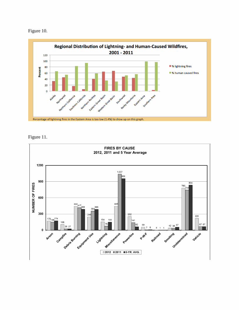

+++++++++++++++++++++++++++++++
Risk of pine beetles increase on forests with no thinning
Pine beetles have killed millions of trees in Canada and in the United States Foresters and
entomologists know that pine beetle outbreaks are cyclical in nature When pine trees are under
stress they attract pine beetles Trees undergo stress when they are too close together (ie too
dense) and things get worse when there is a drought Once conditions are right the beetles thrive
in stressed trees and the progeny attack more trees and the domino effect begins Foresters and
ecologists know that pine beetle cycles have occurred naturally over thousands of years
Figure 14
One factor that increases the risk of a beetle outbreak are policies that do not permit the thinning
of trees State and national forestry organizations know the risk of a beetle outbreak is higher in
counties occupied by National Forests For example in Texas the US Forest Service says that
ldquoVery little suppression took place during the last outbreak A majority of those treatments were
designed to protect RCW habitat as mandated by the Endangered Species act SPB were left
alone in most of the wilderness and killed large acreagesrdquo In contrast some ldquoenvironmentalrdquo
groups object to beetle suppression methods that involve cutting trees in wilderness areas As a
result thinning operations are delayed beetle attack stressed trees and then large populations of
beetles spread to adjacent privately-owned forests After the trees die the risk of wildfire
increases Wildfires start (due to carelessness or accidents or arson) and large expenditures are
made to put the fire out Journalists then report that carbon dioxide caused the inferno The
public concern over wildfires might cause some in Washington to want to increase the cost of
energy For example this month my electrical cooperative sent me an e-mail suggesting that
new EPA regulations could increase my bill by 50 Of course we know that increasing the cost
of energy will hurt the poor more than the wealthy
Figure 15
Foresters tell the public that the best way to prevent a beetle outbreak is to thin the forest to will
increase tree health We also know that planting too many seedlings per acre will also increase
the risk of beetles
httpwwwforestrystatealusPublicationsTREASURED_Forest_Magazine200520Summer
How20to20Grow20Beetle20Bait20-20Revisitedpdfly-owned forests
In contrast the public also tells foresters how to manage beetle risks in wilderness areas The
following is just two pages of a seven-page document illustrating how much time and man-hours
are wasted before operations to reduce the risk of pine beetles can precede in wilderness areas
+++++++++++++++++++++++++++++++
Dr South offers a bet on sea level rise for year 2024
In the past I have had the good fortune to make a few bets with professors
(httpwwwaaesauburneducommpubshighlightsonlinesummer99southhtml) For example
I won a bet on the future price of oil and was successful in betting against Dr Julian Simon on
the price of sawtimber (ie he sent me a check a year after making the bet) Five years ago I
offered to bet on an ldquoice freerdquo Arctic by the summer of 2013 but a BBC journalist [who wrote a
2007 article entitled ldquoArctic summers ice-free lsquoby 2013rsquo rdquo] and several ice experts declined my
offer To date the number of bets I have made has been limited since I have a hard time finding
individuals who are confident enough to make a wager on their predictions
I would like to take this opportunity to offer another ldquoglobal warmingrdquo bet This time the
outcome will be based on sea level data for Charleston SC Recently I was told that ldquoIf we do
nothing to stop climate change scientific models project that there is a real possibility of sea
level increasing by as much as 4 feet by the end of this centuryrdquo
At Charleston the rate of increase in sea level has been about 315 mm per year A four foot
increase (over the next 86 years) could be achieved by rate of 14 mm per year I am willing to
bet $1000 that the mean value (eg the 310 number for year 2012 in Figure 16) will not be
greater than 70 mmyr for the year 2024 I wonder is anyone really convinced the sea will rise
by four feet and if so will they take me up on my offer Dr Julian Simon said making bets was
a good way to see who was serious about their beliefs and who is just ldquotalking the talkrdquo
Figure 16
Annual change in sea level at Charleston SC
Figure 17
httptidesandcurrentsnoaagovsltrendssltrends_stationshtmlstnid=8665530
Selected References
Arno SF 1980 Forest fire history in the northern Rockies Journal of Forestry 78460-465
Botts H Jeffery T Kolk S McCabe S Stueck B Suhr L 2013 Wildfire hazard risk Report
Residential Wildfire Exposure Estimates for the Western United States CoreLogic Inc httpwwwcorelogiccomabout-usresearchtrendswildfire-hazard-risk-reportaspx
Dennison PE Brewer SC Arnold JD Moritz MA 2014 Large wildfire trends in the
western United States 1984ndash2011 Geophysical Research Letters
Guyette RP Spetich MA Stambaugh MC 2006 Historic fire regime dynamics and forcing
factors in the Boston Mountains Arkansas USA Forest Ecol Manage 234293ndash304
Hao Z AghaKouchak A Nakhjiri N Farahmand A 2014 Global integrated drought
monitoring and prediction system Scientific Data 1 Article number 140001
Layser EF 1980 Forestry and climatic change Journal of Forestry 78678-682
Meyn A Schmidtlein S Taylor SW Girardin MP Thonicke K Cramer W 2013
Precipitation-driven decrease in wildfires in British Columbia Regional Environmental
Change 13(1) 165-177
Stein SM Menakis J Carr MA Comas SJ Stewart SI Cleveland H Bramwell L Radeloff
VC 2013 Wildfire wildlands and people understanding and preparing for wildfire in the
wildland-urban interfacemdasha Forests on the Edge report Gen Tech Rep RMRS-GTR-299 Fort
Collins CO US Department of Agriculture Forest Service Rocky Mountain Research Station
36 p
Stephens SL Mclver JD Boerner REJ Fettig CJ Fontaine JB Hartsough BR Kennedy PL
Dylan WS 2012 Effects of forest fuel-reduction treatments in the United States Bioscience
63549-560
Swetnam T Baisan C 1996 Historical fire regime patterns in the southwestern United States
since AD 1700 In CD Allen (ed) Fire Effects in Southwestern Fortest Proceedings of the 2nd
La Mesa Fire Symposium pp 11-32 USDA Forest Service Rocky Mountain Research Station
General Technical Report RM-GTR-286
LETTERS
What If Our GuessesAre Wrong
This old professor would like to com-ment on four ldquoclimate changerdquo articles A1973 article entitled ldquoBrace yourself foranother ice agerdquo (Science Digest 5757ndash61)contained the following quote ldquoMan isdoing these thingshellip such as industrial pol-lution and deforestation that have effects onthe environmentrdquo A 1975 article aboutldquoWeather and world foodrdquo (Bulletin of theAmerican Meteorological Society 561078ndash1083) indicated the return of an ice agewould decrease food production The au-thor said ldquothere is an urgent need for a bet-ter understanding and utilization of infor-mation on weather variability and climatechangehelliprdquo Soon afterwards Earle Layserwrote a paper about ldquoForests and climaterdquo(Journal of Forestry 78678ndash682) The fol-lowing is an excerpt from his 1980 paperldquoOne degree [F] may hardly seem signifi-cant but this small change has reduced thegrowing season in middle latitudes by twoweeks created severe ice conditions in theArctic caused midsummer frosts to returnto the upper midwestern United States al-tered rainfall patterns and in the winter of1971ndash1972 suddenly increased the snowand ice cover of the northern hemisphere byabout 13 percent to levels where it has sinceremainedrdquo (Bryson 1974) Spurr (1953) at-tributed significant changes in the forestcomposition in New England to mean tem-perature changes of as little as 2 degreesGenerally the immediate effects of climaticchange are the most striking near the edge ofthe Arctic (Sutcliffe 1969 p 167) wheresuch things as the period of time ports areice-free are readily apparent However otherexamples cited in this article show that sub-tle but important effects occur over broadareas particularly in ecotonal situations suchas the northern and southern limits of theboreal forest or along the periphery of a spe-ciesrsquo range
Among these papers Layserrsquos paper hasbeen cited more often ( 20 times) but forsome reason it has been ignored by several
authors (eg it has not been cited in anyJournal of Forestry papers) Perhaps it is for-tunate that extension personnel did notchoose to believe the guesses about a comingice age If they had chosen this ldquoopportunityfor outreachrdquo landowners might have beenadvised to plant locally adapted genotypesfurther South (to lessen the impendingthreat to healthy forests) Since the coolingtrend ended such a recommendation wouldhave likely reduced economic returns for thelandowner
A fourth article was about ldquostate serviceforestersrsquo attitudes toward using climate andweather informationrdquo (Journal of Forestry1129ndash14) The authors refer to guessesabout the future as ldquoclimate informationrdquoand in just a few cases they confuse thereader by mixing the terms ldquoclimaterdquo andldquoweatherrdquo For example a forecast that nextwinter will be colder than the 30-year aver-age is not an example of a ldquoseasonal climateforecastrdquo Such a guess is actually a ldquoweatherforecastrdquo (like the ones available from wwwalmanaccomweatherlongrange) Every-one should know that the World Meteoro-logical Organization defines a ldquoclimate nor-malrdquo as an average of 30 years of weather data(eg 1961ndash1990) A 3-month or 10-yearguess about future rainfall patterns is tooshort a period to qualify as a ldquofuture climateconditionrdquo Therefore young foresters (50years old) are not able to answer the questionldquohave you noticed a change in the climaterdquosince they have only experienced one climatecycle They can answer the question ldquohaveyou noticed a change in the weather overyour lifetimerdquo However 70-year-olds cananswer the question since they can comparetwo 30-year periods (assuming they stillhave a good memory)
Flawed computer models have overesti-mated (1) the moonrsquos average temperature(2) the rate of global warming since the turnof the century (3) the rate of melting of Arc-tic sea ice (4) the number of major Atlantichurricanes for 2013 (5) the average Febru-ary 2014 temperature in Wisconsin (136degC) etc Therefore some state service forest-ers may be skeptical of modelers who predict
an increase in trapped heat and then a fewyears later attempt to explain away theldquomissing heatrdquo Overestimations might ex-plain why only 34 out of 69 surveyed forest-ers said they were interested in ldquolong-rangeclimate outlooksrdquo Some of us retired forest-ers remember that cooling predictions madeduring the 1970s were wrong Even ldquointer-mediate-termrdquo forecasts for atmosphericmethane (made a few years ago with the aidof superfast computers) were wrong There-fore I am willing to bet money that theldquolong-range outlooks of climate suitabilityrdquofor red oak will not decline by the amountpredicted (ie tinyurlcomkykschq) I dowonder why 37 foresters (out of 69 sur-veyed) would desire such guesses if outreachprofessionals are not willing to bet money onthese predictions
I know several dedicated outreach per-sonnel who strive to provide the public withfacts regarding silviculture (eg on mostsites loblolly pine seedlings should be plantedin a deep hole with the root collar 13ndash15 cmbelowground) However if ldquoright-thinkingrdquooutreach personnel try to convince land-owners to alter their forest managementbased on flawed climate models then I fearpublic support for forestry extension mightdecline I wonder will the public trust us ifwe donrsquot know the difference between ldquocli-materdquo and ldquoweatherrdquo wonrsquot distinguish be-tween facts and guesses and wonrsquot betmoney on species suitability predictions forthe year 2050
David B SouthPickens SC
Unsafe PracticesOn the cover of the January 2014 issue
I see at least a bakerrsquos dozen foresters andloggers standing in the woods and not a sin-gle hardhat is in sight
We often hear how we should be men-toring young people and new foresters Idonrsquot believe unsafe practices should bechampioned on the cover of American for-estryrsquos principal publication
Douglas G TurnerNewtown PA
258 Journal of Forestry bull May 2014
NZ JOURNAL OF FORESTRY November 2009 Vol 54 No 36
Some foresters are concerned about increasing CO2 levels in the atmosphere while others doubt that CO2 has been the main driver of climate change over the
past million years or over the past two centuries (Brown et al 2008) We three admit that (1) we do not know what the future climate will be in the year 2100 (2) we do not pretend to know the strength of individual feedback factors (3) we do not know how much 600 ppm of CO2 will warm the Earth and (4) we do not know how the climate will affect the price of pine sawlogs in the year 2050 (in either relative or absolute terms) The climate is not a simple system and therefore we believe it is important to ask questions The following 15 questions deal mainly with global climate models (GCM)
A LIST OF QUESTIONS
1 Have any of the climate models been verified
Relying on an unverified computer model can be costly NASA relies on computer models when sending rockets to Mars and the model is verified when the landing is successful However when using one unverified computer model a $125 million Mars Climate Orbiter crashed on September 23 1999 The model was developed by one team of researchers using English units while another used metric units This crash demonstrates how costly an unverified computer model can be to taxpayers At the time Edward Weiler NASArsquos Associate Administrator for Space Science said ldquoPeople sometimes make errorsrdquo
Is it possible that people sometimes make errors when developing complex models that simulate the Earthrsquos climate Is it possible that some models might have ldquocause and effectrdquo wrong in the case of feedback from clouds Is it possible to construct models that produce precise (but inaccurate) estimates of temperature in the future Do some researchers believe in computer predictions more than real data
A report by the International Panel on Climate Change (IPCC) shows a predicted ldquohot zonerdquo in the troposphere about 10 km above the surface of the equator (IPCC 2007b Figure 91f) Why has this ldquohot zonerdquo not been observed We do not know of any paper that reports the presence of this theoretical hot spot Is the absence of this hot zone (Douglass et al 2007) sufficient to invalidate the climate
models If not why not
---------------------
IPCC figure TS26 includes computer projections of four CO2 emission scenarios for the years 2000 to 2025 (IPCC 2007a) Figure 1 is an updated version with extra data points The mean of the projections for global temperatures are jagged suggesting that for some years the temperature is predicted to increase (eg 2007) while in others the temperature is predicted to decline slightly (eg 2008) However observed data for 2006 2007 and 2008 all fall below the projections Although several models suggest the temperature for 2008 should be about 059 degC above the 1961-1990 mean the value in 2008 was 0328degC (are all three digits past the decimal point significant) Although we should not expect any given year to lie on the line this value is outside the range of ldquouncertaintyrdquo listed for green red and blue lines and is almost outside the uncertainty range for the orange line If the observed data falls outside the range of uncertainty for eight years into the future why should foresters be ldquobelieverdquo the models will be accurate (ie lie within the uncertainty bar) 100 years into the future At what point do we admit the Earthrsquos climate is not tracking with the ldquovirtualrdquo climate inside a computer Is the theoretical ldquohot spotrdquo above the equator a result of programming error More importantly how much money are foresters willing to spend on the output of unverified computer models
2 Is it possible to validate climate models
ldquoVerification and validation of numerical models of natural systems is impossible This is because natural systems are never closed and because model results are always non-unique Models can be confirmed by the demonstration of agreement between observation and prediction but confirmation is inherently partial Complete confirmation is logically precluded by the fallacy of affirming the consequent and by incomplete access to natural phenomena Models can only be evaluated in relative terms and their predictive value is always open to question The primary value of models is heuristicrdquo (Oreskes et al 1994)
3 How accurate are the predictions of climate models
Australian Bureau of Meteorology uses computer models to project weather outlook for three months into the future The Bureaursquos web page states that ldquoThese outlooks should be used as a tool in risk management and decision making The benefits accrue from long-term use say over ten years At any given time the probabilities may seem inaccurate but taken over several years the advantages of taking
1David South is a Forestry Professor at Auburn University Bill Dyck is a Science and Technology Broker who has worked for the plantation forest industry and Peter Brown is a Registered Forestry Consultant The authorsrsquo statements should not be taken as representing views of their employers or the NZIF Full citations may be found at
httpsfpauburnedusfwssouthcitationshtml
Some basic questions about climate modelsDavid B South Peter Brown and Bill Dyck1
Professional paper
NZ JOURNAL OF FORESTRY November 2009 Vol 54 No 3 7
account of the risks should outweigh the disadvantagesrdquo Is this statement simply a hope or is it supportable by data These computer model predictions can be compared with actual temperature data over a ten year period The results could illustrate if farmers (who invest money based on the predictions) have benefited from the models or have they suffered from use of the models The difference can provide evidence to illustrate if the 3-month forecasts are any better than flipping a coin One reason why many farmers do not use these 3-month forecasts is because in some areas the models are no better than a random guess
Some claim it is more difficult to predict weather three months into the future than it is to predict the climate 100 years into the future We question this belief system What is the record of predicting climate 100 years into the future Which of the 23 climate models is the most accurate when predicting past events Is a complex computer program that predicts the average temperature for NZ in the past more accurate than one that predicts the average temperature for the Earth 100 years from now Which prediction would be more accurate (determined by predicted minus actual degC) Which set of comparisons has the greater standard deviation
We know that climate models can vary widely in their guesses about how much rain a specific region on Earth might receive (Singer 2008) So how accurate are climate models when predicting the past When models predict precipitation for a given location we can compare the prediction with actual records For example Lim and Roderick (2009) provided predictions of annual precipitation for the last three decades of the 20th Century Examination of the output from 39 computer scenarios reveals that predictions of NZ annual precipitation (Figure 2) ranged from 936 mm to 1851mmyr (mean of 1293 mm standard deviation was 226 mm) The recorded mean rainfallprecipitation of 29 AWIS stations (located mostly at towns or cities) for the years 1971-2000 was 1419 mm but the mean of 27 AWIS stations (not including Milford Sound and Mount Cook) was 1115 mm Neither value represents the actual mean precipitation value for NZ in fact we do not know of an accurate estimate One cannot take 268680 km2 and multiply it by some number (say 13 m) to determine the mass of water that fell on NZ in 1999 Of the 39 computer estimates of past NZ precipitation how can we identify the one that is closest to the actual value for NZ if we cannot even determine the actual value
4 Most climate models have clouds as a positive feedback mechanism If clouds actually produce a negative feedback then CO2 caused global warming is a non-issue (ie warming over then next 100 years might be 05 ordmC) Do climate models have clouds modelled correctly
ldquoAll 23 IPCC climate models now exhibit positive cloud and water vapour feedbackrdquo (Roy Spencer personal
Figure 2 A comparison of predicted rainfall from 20 climate models (adapted from Lim and Roderick 2009) There are 39 output scenarios (bars) with some climate models producing seven estimates and some with only one estimate Nobody knows the mass of precipitation that fell on NZ during the 30 year period and therefore we do not know which computer simulation is closest to the actual value for average rainfall in NZ
Figure 1 A comparison of observed surface temperature means (Hadcrut3) with model projections of Hadcrut3 global averages (adapted from Figure TS26 in IPCC technical summary - page 69) Observed annual mean temperatures are shown (black dots) along with decadal averages (1990-2005 line) Multi-model mean projections (2000-2013 lines) from the IPCC (2007a) report for the SRES B1 A1B and A2 scenarios (top three lines) and a ldquocommitmentrdquo scenario The orange ldquocommitmentrdquo curve shows means of 16 model projections of warming if greenhouse gas and aerosol concentrations were held constant from the year 2000 The uncertainty range indicated against the right-hand axis is for the ldquocommitmentrdquo scenario only Observed values for 2006 2007 and 2008 are all below the ldquocommitmentrdquo line and the observed value for 2008 might lie below the uncertainty range
Professional paper
NZ JOURNAL OF FORESTRY November 2009 Vol 54 No 38
communication) Most climate modellers assume that weak warming will decrease the amount of clouds which reduces the albedo of the Earth A lower albedo (ie less cloud cover) results in more warming
In contrast Spencer and Braswell (2008) suggest that clouds likely produce a negative feedback Weak warming seems to increase the amount of clouds which increases the albedo of the Earth (Figure 3) If increases in CO2 results in more clouds this will invalidate most climate models Roy Spencer said that ldquoif feedbacks are indeed negative then manmade global warming becomes for all practical purposes a non-issuerdquo What real-world data prove that increasing CO2 will result in fewer clouds
In 1988 Steven Schneider said ldquoClouds are an important factor about which little is knownrdquo (Revkin 1988) ldquoWhen I first started looking at this in 1972 we didnrsquot know much about the feedback from clouds We donrsquot know any more now than we did thenrdquo
Did climate models have the feedback from clouds correct in 1988 Is the feedback from clouds any different now than it was three decades ago Does the magnetic activity of the sun affect cosmic rays and the formation of clouds (Svensmark and Calder 2007) Do climate modellers include cosmic rays in their models Do climate modellers really believe their 2009 models have the formation of clouds correct in their models
5 Can we estimate how much of the +076degC temperature departure recorded in February 1998 (Figure 4) can be attributed to El Nintildeo and how much can be attributed to the CO2 that originates from burning of fossil fuels
Steven Schneider (Revkin 1988) said ldquoTo begin with the magnitude of the various perturbations (to use the scientistsrsquo delicate word) of the environment are difficult to predict And estimates of even the immediate effects of those perturbations are unreliable Still harder to predict are the ground-level consequences of these effects - for example the number of feet by which sea level will rise given a particular rise in the temperature of the globe or the effects on phytoplankton of a particular increase in ultraviolet radiation caused by a particular reduction in the ozone layer Harder yet to predict - lying really entirely in the realm of speculation - are the synergistic consequences of all or some of these effects And lying completely beyond prediction are any effects that have not yet been anticipatedrdquo
ldquoFor all these reasons the margin for error is immense And that of course is the real lesson to be learned from the worldrsquos earlier attempts at predicting global perils What the mistakes show is that in these questions even the most disinterested and professional predictions are filled with uncertainty Uncertainty in such forecasts is not a detail soon to be cleared up it is part and parcel of the new situation - as inextricably bound up with it as mounting levels of carbon dioxide or declining levels of ozone For
Figure 4 Globally averaged satellite-based temperature of the lower atmosphere (where zero = 20 year average from 1979 to 1998) February 1998 was 076 degC above the 20-year average Data provided by Professors John Christy and Roy Spencer University of Alabama Huntsville
Figure 3 A negative cloud feedback would increase the Earthrsquos albedo (figure provided by Dr Roy Spencer)
Professional paper
NZ JOURNAL OF FORESTRY November 2009 Vol 54 No 3 9
the scientistsrsquo difficulties do not stem merely from some imperfections in their instruments or a few distortions in their computer models they stem from the fundamental fact that at this particular moment in history mankind has gained the power to intervene in drastic and fateful ways in a mechanism - the ecosphere - whose overall structure and workings we have barely begun to grasprdquo
6 How did the IPCC determine that it is extremely unlikely that warming in the past 50 years was caused by natural fluctuations
Table 94 in WG1 (page 792 IPCC 2007b) provides a synthesis of ldquoclimate change detection resultsrdquo Regarding surface temperature the authors state that it is extremely likely (gt95) that ldquowarming during the past half century cannot be explained without external radiative forcingrdquo We wonder exactly what does this statement mean Are the authors simply predicting that researchers (eg Svensmark and Calder 2007 Spencer and Braswell 2008 Klotzbach et al 2009) will never publish papers to suggest that natural variation in clouds could explain the warming
We agree that humans have altered surface temperatures by construction of roads and cities afforestation producing black carbon (ie soot) burning of fuel (which releases heat and water vapour) We have no doubt that temperatures records are biased upwards because of ldquoheat islandsrdquo and because thermometers are often located in improper locations (Klotzbach et al 2009) However it is not clear how the ldquogt95 likelihoodrdquo value was obtained Was it obtained from ldquoan elicitation of expert viewsrdquo (IPCC 2005) or from a quantitative analysis of output from climate models (Tett et al 1999)
7 What system was sampled when declaring an anthropogenic change has been detected with less than 1 probability
In 2001 the IPCC panel concluded that ldquomost of the observed warming over the last 50 years is likely due to increases in greenhouse gas concentrations due to human activitiesrdquo In 2007 the IPCC authors go on to say that ldquoAnthropogenic change has been detected in surface temperature with very high significance levels (less than 1 error probability)rdquo(IPCC 2007b) We wonder how the authors went about calculating a p-value of lt1 if there is confounding between CO2 increases and natural changes in clouds We asked a few IPCC experts they said the p-value was obtained by generating a data set from a computer model In other words you create a virtual world without people generate hypothetical temperatures from the virtual world compare the two sets (virtual world with people and virtual world without people) and then generate a p-value
In 2007 Dr Bob Carter (Adjunct Professorial Research Fellow - James Cook University) wrote ldquoIn the present state
of knowledge no scientist can justify the statement lsquoMost of the observed increase in globally averaged temperature since the mid-20th century is very likely due [90 per cent probable] to the observed increase in anthropogenic greenhouse gas concentrationsrsquo as stated in the IPCCrsquos 2007 Summary for Policy Makersrdquo We agree with Dr Carter We assume that virtual worlds were sampled to determine the 1 probability We claim that the 1 probability was applied to output from climate models and not to replications made from the real world
8 One climate model suggests that increasing the albedo of the Earthrsquos surface from deforestation is stronger than the CO2 effect from deforestation Would harvesting native forests in temperate and boreal zones (plus making wood furniture and lumber from the harvested logs) and converting the land to pastureland cool the Earth
After examining a virtual Earth Bala et al (2007) said ldquoWe find that global-scale deforestation has a net cooling influence on Earthrsquos climate because the warming carbon-cycle effects of deforestation are overwhelmed by the net cooling associated with changes in albedo and evapotranspirationrdquo Has this climate model been verified If an increase the albedo (from deforestation) is more powerful than the CO2 effect (South 2008a) why are albedo credits (South and Laband 2008) not included in Climate Trading Schemes
9 IPCC authors predict an increase in the number of record hot temperatures and that this will often cause a decline in the number of record cold temperatures Are there data to support this claim Is it true that an increase in record high temperatures will result in a decline in record low temperatures
Solomon and others (IPCC 2007a) say that ldquolinking a particular extreme event to a single specific cause is problematicrdquo and we concur However the authors go on to say that ldquoAn increase in the frequency of one extreme (eg the number of hot days) will often be accompanied by a decline in the opposite extreme (in this case the number of cold days such as frosts)rdquo We do not know of a reference to support this claim We question the claim that the probability of a record cold event in January or July is less now than it was in the 19th century In fact in 2009 six US states set cold temperature records (115 year data) for the month of July (IA IL IN OH PA WV) Why did these records occur if the probability of a cold July is less now than it was in 1893
We also question the claim that ldquoIn some cases it may be possible to estimate the anthropogenic contribution to such changes in the probability of occurrence of extremesrdquo How is this possible Other than simply guessing we fail to see how a scientist could estimate an anthropogenic contribution to an increase in frequency of record coldhigh
Professional paper
NZ JOURNAL OF FORESTRY November 2009 Vol 54 No 310
temperatures Rare events do occur in nature Researchers can certainly show a correlation but how would they determine how much of the 076 degC departure in Figure 4 is anthropogenic We ldquoestimaterdquo that 99 of this value is due to El Nintildeo but we admit this estimate can not be verified
Solomon Qin Manning and others suggest temperatures for a given region or for the Earth follow a ldquofamiliar lsquobellrsquo curverdquo and when the climate warms (for whatever reason) the entire distribution is shifted to the right (Figure 5) They suggest that a histogram of the pattern of temperature occurrences is similar for both the ldquoprevious climaterdquo
and the ldquonewrdquo warmer climate We propose an alternate hypothesis (Figure 6) The distribution is negatively skewed with the tails about the same as before A third hypothesis suggests that the warmed distribution becomes negatively skewed and flatter (ie platykurkic) This hypothesis is supported by predictions of ocean temperatures by the Max Planck Institute (National Assessment Synthesis Team 2000 page 83) Are there any actual data to support the IPCC hypothesis that assumes no change in kurtosis or skewness
In Table 1 we provide some extreme high and low temperatures for selected land based locations in the Southern Hemisphere Note that for these locations no record high temperature occurred after 1975 and all but one record low temperature occurred after 1970 The occurrence of extreme low temperatures following record high temperatures in the southern hemisphere is interesting especially since this is counter to the ldquono change in skew or kurtosisrdquo hypothesis The theory presented in Figure 5 suggests a 0 probability of a record extreme cold event occurring after global warming
We predict that one or more of the records in Table 1 will be broken by the year 2100 If Antarctica drops below -90 degC someone might claim it was caused by humans (perhaps due to chemicals depleting the ozone layer) Likewise if a record high temperature occurs in Australia or New Zealand we will likely read that it was caused by humans The experts
Figure 6 Histogram showing actual data (N = 367) from satellites over the period (December 1978 to June 2009) Each solid square represents the number of months that the temperature of the troposphere (above the southern hemisphere oceans) varied from an arbitrary mean value Data (ie solid squares) obtained from the Climate Center University of Alabama at Huntsville (httpwwwncdcnoaagovoaclimateresearchuahncdclt) The dashed line represents a hypothetical distribution from a cooler period in the past In this graph the tails from both curves are deliberately identical The hypothetical line was drawn so that the probability of extreme events is not changed
Figure 5 Schematic showing the IPCC view that little or no skew and kurtosis occurs when the mode shifts by +07 degC The authors suggest the probability of extreme low temperatures decrease in proportion to the probability of high temperature (Figure 1 Box TS5 from IPCC 2007a)
Table 1 Dates of record high and low temperatures for some southern hemisphere locations (as of December 2008) Note that in these cases the record low temperature occurred after the record high temperature Although these records do not prove anything they are not hypothetical Note that no record high temperature occurred after 1975 and all record low temperatures but one occur after 1970
Countrylocation Record degC Date
Antarctica High 146 5 January 1974
Low -892 21 July 1983
Argentina High 489 11 December 1905
Low -33 1 June 1907
Australia High 507 2 January 1960
Low -23 29 June 1994
New Zealand High 424 7 February 1973
Low -216 3 July 1995
South Africa High 50 3 November 1918
Low -186 28 June 1996
South America High 491 2 January 1920
Low -39 17 July 1972
Professional paperProfessional paper
NZ JOURNAL OF FORESTRY November 2009 Vol 54 No 3 11
quoted might even take an unscientific approach and provide a probability in an attempt to prove the event was anthropogenic
10 Solar irradiance that reaches the Earthrsquos surface has declined since 1950 How much of reduction in irradiance is due to an increase in clouds and how much is due to an increase in pollution (ie soot and aerosols)
ldquoAs the average global temperature increases it is generally expected that the air will become drier and that evaporation from terrestrial water bodies will increase Paradoxically terrestrial observations over the past 50 years show the reverserdquo (Roderick and Farquhar 2002) How much of the ldquoglobal dimmingrdquo (Stanhill 2005) is due to humans caused air pollution and how much is due to a negative feedback from clouds
11 Why do some forest researchers use statistical downscaling approaches when the scenarios have largely been regarded as unreliable and too difficult to interpret
Wilby and others (2004) have pointed out that some modellers combine coarse-scale (ie hundreds of kilometres) global climate models with higher spatial resolution regional models sometimes having a resolution as fine as tens of kilometres Most of the statistical downscaling approaches ldquoare practiced by climatologists rather than by impact analysts undertaking fully fledged policy oriented impact assessments This is because the scenarios have largely been regarded as unreliable too difficult to interpret or do not embrace the range of uncertainties in GCM projections in the same way that simpler interpolation methods do This means that downscaled scenarios based on single GCMs or emission scenarios when translated into an impact study can give the misleading impression
of increased resolution equating to increased confidence in the projectionsrdquo (Wilby et al 2004)
12 When comparing similar locations and the same number of weather stations in NZ has the average temperature changed much since 1860
We agree that natural events affect the Earthrsquos temperature (eg McLean et al 2009) We also agree that human activities such as deforestation afforestation irrigation road construction city construction etc can alter the albedo of the Earthrsquos surface However we are uncertain that average temperatures experienced in NZ during 1971 to 2000 are that much different than the temperatures experienced from 1861 to 1866 (Table 2) Why do temperatures records from Hokitika NZ (since 1866) show no increase in temperature (Gray 2000)
Predicted annual temperature changes (in degC) relative to 1980-1999 have been predicted for 12 climate models (Table A21 Ministry for the Environment 2008) All 12 models predict an increase in temperature for NZ (for the period 2030 to 2049) A German model predicts only a 033 degC increase while a Japanese model predicts a 2 degC increase In contrast an older model (of unknown origin) predicts that NZ will be cooler in July 2029 than it was in July of 1987 (Revkin 1988) There are only about two decades to go before the year 2030 so it will be interesting to see which of the 13 models is closest to the observed data When compared to 1987 will NZ be cooler in the winter of 2028 than most other locations in the world (Revkin 1988) or will it be about 2 degC warmer (eg miroc32 hires)
13 Do outputs from climate models allow some researchers to selectively ignore real-world observations
Farman et al (1985) were the first to report a reduction
Table 2 A comparison of temperature data from five locations in New Zealand with predicted temperature in 2040 Pre-1868 data are from New Zealand Institute Transactions and Proceedings 1868 (httptinyurlcom7ycpl6) and post-1970 data are from National Institute of Water and Air Research (httptinyurlcoma5nj3c) Guesses for annual mean temperature for the year 2040 are in brackets (from Table 22 Ministry for the Environment 2008) Table adapted from Vincent Gray
Station Years of data Before 1867 Years of data 1971-2000 2040
degC degC degC
Auckland 15 157 25 151 [160]
Taranaki - New Plymouth 12 137 20 136 [145]
Nelson 16 128 25 126 [135]
Christchurch 11 128 26 121 [130]
Dunedin 15 104 26 110 [119]
Mean 131 129
Professional paperProfessional paper
NZ JOURNAL OF FORESTRY November 2009 Vol 54 No 312
in the Antarctic ozone hole Some experts at first dismissed the observations of the British scientist since Farmanrsquos findings differed with predictions generated using NASA computer models (Schell 1989) This is not the only case where output from an unverified computer model was initially given more credence than actual observations Recently Svensmark and Calder (2007) provide data to propose a new theory of global warming Have researchers relied on an unverified computer model to disprove a new theory of climate change (Pierce and Adams 2009)
14 Do foresters rely on predicted timber prices that are generated from combining three complex computer models
A climate model a biogeochemistry model and an economics model were used to predict standing timber prices for the United States (Joyce et al 2001) Prices were predicted to increase by 5 to 7 from 2000 to 2010 but no error bars were included the graph In contrast actual prices for standing sawlogs in 2009 are generally lower than they were in 2000 (in some cases 40 lower) Would any forestry consultant rely on 10-year price forecasts generated by combining three complex computer models Do researchers actually believe they can determine what the price of standing timber would be in the year 2050 if CO2 levels in the atmosphere were kept at 355 ppmv (Ireland et al 2001)
15 To capture the public imagination should foresters offer up scary scenarios
Stephen Schneider (Schell 1989) said ldquoas scientists we are ethically bound to the scientific method in effect promising to tell the truth the whole truth and nothing but - which means that we must include all the doubts the caveats the ifs ands and buts On the other hand we are not just scientists but human beings as well And like most people wersquod like to see the world a better place which in this context translates into our working to reduce the risk of potentially disastrous climatic change To do that we need to get some broad-based support to capture the
publicrsquos imagination That of course entails getting loads of media coverage So we have to offer up scary scenarios make simplified dramatic statements and make little mention of any doubts we might have This lsquodouble ethical bindrsquo we frequently find ourselves in cannot be solved by any formula Each of us has to decide what the right balance is between being effective and being honest I hope that means being bothrdquo
Conclusions
We are concerned the scientific method is being downplayed in todayrsquos world Hypothesis testing is an irreplaceable tool in science but some no longer test hypothesis and others do not declare their doubts Now all that is needed to set policy is an unverified computer model some warnings about the future some name calling and a good marketing program Debate is essential to scientific progress but it seems it is no longer in vogue Sometimes those who ask questions (like the 15 above) are ignored suppressed or attacked with name calling (eg see Witze 2006 Seymour and Gainor 2008 South 2008b)
Our profession should be a place where questions about computer models (either process based forestry models or three-dimensional climate models) are welcomed Debate should be encouraged and hypotheses should be tested (not simply proposed) However it now seems a number of researchers and foresters have accepted the hypothesis that CO2 is the primary driver of a changing climate Some ignore factors such as changes in cloud cover changes in surface albedo (Gibbard et al 2005) changes in cosmic rays increases in soot (in air and on ice) and the Pacific Decadal Oscillation Ignoring these factors appears to be driven by the idea that the Earthrsquos complex climate system is relatively easy to control by planting more trees on temperate and boreal grasslands
We hope our profession will rise above soothsaying and will encourage debate on topics and policies that affect our forests As NZIF members if we choose not to question authority we might be accused of violating our code of ethics
Professional paper
What if Climate Models are wrong
People who trust IPCC climate projections (eg Figure 1) also believe that Earths atmospheric Greenhouse Effect is a radiative phenomenon and that it is responsible for raising the average surface temperature by 33degC compared to an airless environment According to IPCC Third Assessment Report (2001) For the Earth to radiate 235 watts per square meter it should radiate at an effective emission temperature of -J9degC with typical wavelengths in the infrared part of the spectrum This is 33degC lower than the average temperature of J4degC at the Earths surface Mainstream climate science relies on a simple formula based on Stefan-Boltzmann (S-B) radiation law to calculate Earths average temperature without an atmosphere (ie -19degC) This formula is also employed to predict Moons average temperature at -20 C (253K) (eg NASA Planetary Fact Sheet) But is the magnitude of the atmospheric greenhouse effect really 33 C What if the surface temperature of Earth without an atmosphere were much colder What if the popular mean temperature estimate for the Moon were off by more than 50 C
Although we cannot experimentally verify the -19 C temperature prediction for a hypothetical airless Earth we could check if the predicted -20 C average temperature for the Moon is correct After all the Moon can be viewed as a natural grey-body equivalent of Earth since it orbits at the same distance from the Sun and has virtually no atmosphere (the gas pressure at the lunar surface is only about 3 x 10⁻¹⁰ Pa) Recent data from the Diviner instrument aboard NASAs Lunar Reconnaissance Orbiter as well as results from detailed thermo-physical models (eg Vasavada et al 19992012) indicate that the Moon average surface temperature is actually -76 C (1973K) Diviner measurements discussed by Vasavada et al (2012) show that even at the lunar equator (the warmest latitude on the Moon) the mean annual temperature is -60 C (213K) or 40 C cooler than the above theoretical global estimate Why such a large discrepancy between observed and calculated lunar temperatures
According to a new analysis by Volokin amp ReLlez (2014) climate scientists have grossly overestimated Moons average temperature and Earths black body temperature for decades due to a mathematically incorrect application of the S-B law to a sphere The current approach adopted by climate science equates the mean physical temperature of an airless planet (Tgb K) with its effective emission temperature (Te K) calculated from the equation
(1)
where So is the solar irradiance (W m-2) ie the shortwave flux incident on a plane
perpendicular to solar rays above the planets atmosphere a p is the planet average shortwave albedo E is the surface thermal emissivity (095 = E = 099) and (J = 56704xlO-8 W m-2 K-4 is the
1
12
- Model Average 09
-0- Avg of two Satellite datasets
Avg of four Balloon datasets
06 The finear trend of aU tim e series intersectsat ze ro at 1979 with the
c values shown as drpartures from that trilnd line
01
IReal World J
00
IGIObal Mid-Tropospheric Tem perat ure S-year averages
-03 1975 1980 1985 1990 1995 2000 2005 2010 2015 2020 2025
IA THE UN IVERSITY OF
A LABAMA IN HUNTSV ILLE
Figure 1 Model projections of global mid-tropospheric temperature (red line) compared to observed temperatures (blue and green lines) Figure courtesy of Dr John Christy
S-B constant The factor V4 serves to re-distribute the solar flux from a flat surface to a sphere It arises from the fact that the surface area of a sphere (4nR2) is 4 times larger than the surface area of a flat disk (7CR2) with the same radius R Inserting appropriate parameter values for Earth in Eq (1) ie So = 13617 W m-2 ap = 0305 and E = 10 produces Te = 2542K (-19 C) which is the basis for the above IPCC statement We note that the -20 C (253K) temperature estimate for the Moon is obtained from Eq (1 ) using ap = 0305 which is Earths albedo that includes the effect of clouds and water vapor on shortwave reflectivity However the correct albedo value is the Moon 01 2 - 013 which yields ~270 K (- 3 C) for the Moon average temperature according to Eq (1)
Equation (1) employs a spatially averaged absorbed solar flux to calculate a mean surface temperature This implies a uniform distribution of the absorbed solar energy across the planet surface and a homogeneous temperature field However these assumptions are grossly inaccurate because sunlight absorption on a spherical surface varies greatly with latitude and time of day resulting in a highly non-uniform distribution of surface temperatures This fact along with the non-linear (4th root) dependence of temperature on radiative flux according to S-B law creates a relationship known in mathematics as Holders inequality between integrals (eg Abualrub and Sulaiman 2009 Wikipedia Holders inequality) Holders inequality applies to certain types of non-linear functions and states that in such functions the use of an arithmetic average for the independent distributed variable will not produce a physically
2
correct mean value for the dependent variable In our case due to a non-linear relationship between temperature and radiative flux and a strong dependence of the absorbed solar flux on latitude one cannot correctly calculate the true mean temperature of a uni-directionally illuminated planet from the spatially averaged radiative flux as attempted in Eq (1) Due to Holders inequality the effective emission temperature produced by Eq (1) will always be significantly higher than the physical mean temperature of an airless planet ie Te raquo Tgb
Volokin amp ReLlez (2014) showed that in order to derive a correct formula for the mean physical temperature of a spherical body one must first take the 4th root of the absorbed radiation at every point on the planet surface and then average (integrate) the resulting temperature field rather than calculate a temperature from the spatially averaged solar flux as done in Eq (1) Using proper spherical integration and accounting for the effect of regolith heat storage on nighttime temperatures Volokin amp ReLlez (2012) derived a new analytical formula for the mean surface temperature of airless planets ie
(2)
where ltIgt(1Je) is given by
ltIgt(1Je) = (1 -1Je)025 + 0931 1Je 025 (3)
Here ae is the effective shortwave albedo of the planet surface 1Je (eta) is the effective fraction of absorbed solar flux stored as heat in the regolith through conduction and ltIgt(1Je) 10 is a dimensionless scaling factor that boosts the average global temperature above the level expected from a planet with zero thermal inertia ie if the surface were completely nonshyconductive to heat Thanks to 1Je gt 0 (non-zero storage of solar energy in the regolith) the night side of airless celestial bodies remains at a significantly higher temperature than expected from the cosmic microwave background radiation (CMBR) alone This increases the mean global planetary temperature The fraction of solar flux stored in regolith can theoretically vary in the range 00 1Je 10 In reality however due to physical constrains imposed by the regolith thermal conductivity this range is much narrower ie 0005 lt 1Je lt 0015 which limits the temperature enhancement factor to 125 lt ltIgt(1Je) lt 132 According to Eq (3) ltIgt(1Je) has a non-linear dependence on 1Je - it increases for 00 1Je 05 and decreases when 05 1Je 10 reaching a maximum value of 1627 at 1Je = 05 However since it is physically impossible for a planets regolith to store on average as much as 50 of the absorbed solar flux as heat ltIgt(1Je) cannot practically ever reach its theoretical maximum
Independent thermo-physical calculations along lunar latitudes yielded 1Je = 000971 for the Moon hence ltIgt(1Je) = 129 according to Eq (3) Due to the lack of moisture and convective heat transport between soil particles in an airless environment the apparent thermal conductivity of the regolith of celestial bodies without atmosphere is much lower than that on Erath resulting in values for 1Je close to 001 Volokin amp ReLlez (2014) showed that Eq (2) quite accurately predicts Moons true average surface temperature of 1973 K (within 025 K)
2using observed and independently derived values for So = 13617 W m- ae = 013 and
3
E = 098 and TJe In general Fonnula (2) is expected to be valid for any airless spherical body provided So 015 W m-2
If solar irradiance is lower than 015 W m-2 then the relative
contribution ofCMBR to planets temperature becomes significant and another more elaborate fonnula for Tgb needs be used (see Volokin amp ReLlez 2014)
Equation (2) demonstrates that Tgb is physically incompatible with Te via the following comparison Using So = 13617 ae = 013 and E = 098 in Eq (1) yields Te = 2702K for the Moon This estimate is 215K higher than the maximum theoretically possible temperature Tgb = 2487K produced by Eq (2) using the same input parameters and a physically unreachable peak value of ltp(TJ) = 1627 corresponding to TJe = 05 Therefore it is principally impossible for an airless planet to reach an average global temperature as high as its effective emission temperature This renders Te a pure mathematical construct rather than a measurable physical quantity implying that Te is principally different from Tgb and should not be confused it
Earths atmospheric greenhouse effect (AGE) can be measured as a difference between the actual average global surface temperature (Ts) and the mean temperature of an equivalent grey body with no atmosphere orbiting at the same distance from the Sun such as the Moon Adopting Te as the grey-bodys mean temperature however produces a meaningless result for AGE because a non-physical (immeasurable) temperature (Te) is being compared to an actual physical temperature (Ts) Hence the correct approach to estimating the magnitude of AGE is to take the difference between Ts and Tgb ie two physical palatable temperatures Using the current observed average global surface temperature of 144degC (2876K) (NOAA National Climate Data Center Global Surface Temperature Anomalies) and the above estimate of Earths true gray-body mean temperature (ie Moons actual temperature) we obtain AGE =
2876 K - 1973 K = 903 K In other words the greenhouse effect of our atmosphere is nearly 3 times larger than presently assumed This raises the question can so-called greenhouse gases which collectively amount to less than 04 of the total atmospheric mass trap enough radiant heat to boost Earths average near-surface temperature by more than 90 K Or is there another mechanism responsible for this sizable atmospheric thennal effect in the lower troposphere Observations show that the lower troposphere emits on average 343 W m-2 of long-wave radiation towards the surface (eg Gupta et al 1999 Pavlakis et al 2003 Trenberth et al 2009) Such a thennal flux is 44 larger than the global averaged solar flux absorbed by the entire Earth-atmosphere system (ie 238-239 W m-2
) (Lin et al 2008 Trenberth et al 2009) This fact implies that the lower troposphere contains more kinetic energy than can be accounted for by the solar input alone Considering the negligible heat storage capacity of air these measurements suggest the plausibility of an alternative non-radiative AGE mechanism Consequently if another major AGE mechanism existed that is not considered by the current climate science what would this imply for the reliability and accuracy of climate-model projections based on the present radiative Greenhouse paradigm
In closing we concur with physicist and Nobel Prize laureate Richard Feynman who said It does not make any difference how beautiful your guess is it does not make any difference how smart you are who made the guess or what his name is - if it disagrees with experiment it is wrong That is all there is to it (1964 lecture at Cornell University)
4
5
References Abualrub NS and WT Sulaiman (2009) A Note on Houmllders Inequality International Mathematical Forum 4(40)1993-1995 httpwwwm-hikaricomimf-password200937-40-2009abualrubIMF37-40-2009-2pdf Gupta S K Ritchey N A Wilber A C and Whitlock C A (1999) A Climatology of Surface Radiation Budget Derived from Satellite Data J Climate 12 2691ndash2710 IPCC Third Assessment Report (2001) Working Group I The Scientific Basis Chapter 1 httpwwwipccchipccreportstarwg1pdfTAR-01PDF Lin B Paul W Stackhouse Jr Patrick Minnis Bruce A Wielicki Yongxiang Hu Wenbo Sun Tai-Fang Fan and Laura M Hinkelman (2008) Assessment of global annual atmospheric energy balance from satellite observations J Geoph Res Vol 113 p D16114 NASA Planetary Facts Sheet (httpnssdcgsfcnasagovplanetaryfactsheet) NOAA National Climate Data Center Global Surface Temperature Anomalies (httpwwwncdcnoaagovcmb-faqanomaliesphp) Pavlakis K G D Hatzidimitriou C Matsoukas E Drakakis N Hatzianastassiou and I Vardavas (2003) Ten-year global distribution of downwelling longwave radiation Atmos Chem Phys Discuss 3 5099-5137 Trenberth KE JT Fasullo and J Kiehl (2009) Earthrsquos global energy budget BAMS March311-323 Vasavada A R J L Bandfield B T Greenhagen P O Hayne M A Siegler J-P Williams and D A Paige (2012) Lunar equatorial surface temperatures and regolith properties from the Diviner Lunar Radiometer Experiment J Geophys Res 117 E00H18 doi1010292011JE003987 Vasavada A R D A Paige and S E Wood (1999) Near-surface temperatures on Mercury and the Moon and the stability of polar ice deposits Icarus 141 179ndash193 doi101006icar19996175 Volokin D and ReLlez L (2014) On the Average Temperature of Airless Spherical Bodies and the Magnitude of Earths Atmospheric Thermal Effect (under review) Wikipedia Houmllders inequality (httpenwikipediaorgwikiHC3B6lders_inequality)
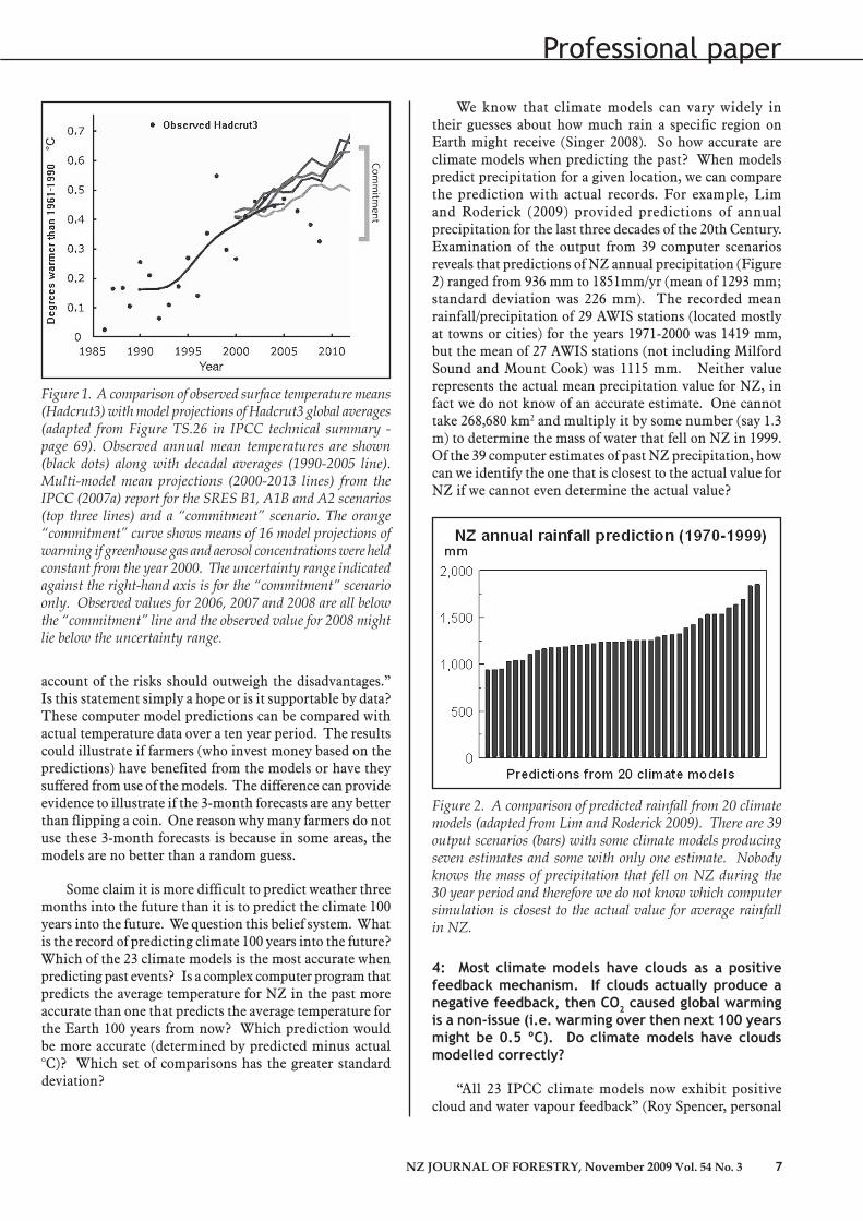