texas water resources institute annual technical … water resources institute annual technical...

Texas Water Resources Institute Annual Technical Report

FY 2002

Introduction

Research ProgramDuring 2002-03, TWRI supported 10 research projects to graduate students at 6 universities in Texas,including Texas A&M University, Baylor University, Rice University, West Texas A&M University, theUniversity of Texas at Austin, and Texas Tech University.

In broad terms, these studies focused on such broad issues as irrigation (1 study), water quality (5 studies),wastewater (3 studies), aquatic biology (1 study), flooding and runoff (2 studies), computer modeling (3studies), bays (1 study), wetlands (1 study) and human health (1 study).

Nyland Falkenberg of Texas A&M University carried out field research in South Texas (Uvalde) todevelop improved technologies to manage irrigation needs and control biological stressors facingagricultural crops. Jordan Furnans of the University of Texas at Austin utilized complex computer modelsto simulate the development of algal blooms off the Texas coast. Jennifer Hadley developed a computersimulation model that will provide real-time estimates of runoff throughout Texas over the World WideWeb. June Wolfe at Baylor is exploring the role of periphyton in processing and removing phosphorusfrom streams using laboratory studies. Jude Benavides of Rice created a high-tech website thatincorporates the latest in computer simulation modeling to provide real-time estimates of flooding indowntown Houston. Judy Vader of Texas A&M University investigated the fate of atrazine in lakesediments at selected sites throughout Texas. Kevin Heflin of West Texas A&M University tested whetherthe use of cattle feeds with reduced phosphorus concentrations might lessen nutrient runoff. Audra Morseof Texas Tech measured concentrations of antibiotics in wastewater plants and effluent runoff in the TexasHigh Plains to determine if there might be possible human health effects. Matthew Simmons of TexasA&M University worked to design and restore a wetland in an urbanized portion of the Dallas, TX area.Amanda Bragg of Texas A&M University determined whether the use of a chemical additive (struvite)might reduce phosphorus runoff from dairy wastes.

Enhanced Flood Warnings for the Texas Medical Center: ASecond Generation Flood Alert System (FAS2)

Basic Information

Title:Enhanced Flood Warnings for the Texas Medical Center: A Second GenerationFlood Alert System (FAS2)

Project Number: 2002TX47B

Start Date: 3/1/2002

End Date: 2/1/2003

Funding Source: 104B

Congressional District:

7th

Research Category: None

Focus Category: Floods, Models, Hydrology

Descriptors: None

Principal Investigators:

Jude A. Benevides, Philip B. Bedient

Publication

1. Benavides, Jude. Enhanced Flood Warnings for the Texas Medical Center: A Second GenerationFlood Alert System (FAS2). Texas Water Resources Institute SR 2003-017.

Title: Enhanced Flood Warnings for the Texas Medical Center: A Second Generation Flood Alert System (FAS2)

Keywords : Flood warning; Flood alert; NEXRAD; Flood protection; Brays Bayou, Texas

Medical Center. Duration: March 2002 – Feb 2003 Federal Funds Requested: $5,000.00 Non-Federal (Matching) Funds Pledged: $10,980.00 Principal Investigator: Jude A. Benavides, Graduate Student, Dept. of Civil and

Environmental Engineering, Rice Univ., MS-317, 6100 Main St., Houston, TX, 77005. E-mail: [email protected]

Ph: 713-348-2398 Co-Principal Investigator: Philip B. Bedient, Ph.D., P.E., Hermann Brown Professor of

Engineering, Dept. of Civil and Environmental Engineering, Rice Univ., E-mail: [email protected]

Congressional District: U.S. Congressional District # 2670

List of Publications Used in this Study:

1. Anagnostou, E.N., W.F. Krajewski, D.J. Seo, E.R. Johnson (1998). "Mean-Field Rainfall Bias Studies for WSR-88D." J. of Hydrol. Eng., 3(3): 149-159.

2. Bedient, P.B., B.C. Hoblit, D.C. Gladwell, and B.E. Vieux (2000). “NEXRAD Radar for Flood Prediction in Houston,” J. of Hydrol. Eng., 5(3): 269 – 277.

3. Bedient, P.B. and W.C. Huber (2002). Hydrology and Floodplain Analysis, 3rd Edition. Prentice Hall Publishing Co., Upper Saddle River, NJ, 763.

4. Benavides, J.A. (2002). “Floodplain Management Issues in Hydrology” Chapter 12 (pp. 682-713) of Hydrology and Floodplain Analysis, 3rd Ed. (P.B. Bedient and W.C. Huber). Prentice-Hall.

5. Borga, M. (2002). "Accuracy of Radar Rainfall Estimates for Streamflow Simulation." J. Hydrol., 267: 26-39.

6. Carpenter, T. M., J. A. Sperfslage, K.P. Georgakakos, T. Sweeney, D.L. Fread (1999). "National threshold runoff estimation utilizing GIS in support of operational flashflood warning systems." J. of Hydrol., 224: 21-44.

7. Carpenter, T.M., K.P. Georgakakos, J.A. Sperfslagea (2001). “On the Parametric and NEXRAD-radar Sensitivities of a Distributed Hydrologic Model Suitable for Operational Use.” J. of Hydrol., 253:169-193.

8. Collier, Christopher G. (1996). Applications of Weather Radar Systems: A Guide to Uses of Radar Data in Meteorology and Hydrology. John Wiley and Sons, Chichester, England.

9. Crosson, W.L., C.E. Duchon, R. Raghavan, and S.J. Goodman. (1996). “Assessment of Rainfall Estimates Using a Standard Z-R Relationship and the Probability Matching Method Applied to Composite Radar Data in Central Florida.” J. of Appl. Meteorol., 35(8): 1203-1219.

10. Crum, T.D., R.L. Alberty, D.W. Burgess (1993). "Recording, Archiving, and Using WSR-88D Data." Bull. Amer. Meteorological Soc., 74(4): 645-653.

11. FEMA and HCFCD (2002). Off the Charts. T.S. Allison Public Report, Harris County Flood Control District, Texas.

12. Finnerty, B., and D. Johnson. (1997). “Comparison of National Weather Service Operational Mean Areal Precipitation Estimates Derived from NEXRAD Radar vs. Rain Gage Networks.” International Association for Hydraulic Research (IAHR) XXVII Congress, San Francisco, California. <http://hsp.nws.noaa.gov/hrl/papers/compar.htm>.

13. HCFCD (2000). Project Brays, Harris County Flood Control District, Texas.

14. Hoblit, B.C., B.E. Vieux, A.W. Holder, and P.B. Bedient, (1999). “Predicting With Precision,” ASCE Civil Engineering Magazine, 69(11): 40-43.

15. Hydrologic Engineering Center (1998), HEC-HMS, Hydrologic Modeling System, U.S. Army Corps of Eng, Davis, CA,

16. Liscum, F., and B.C. Massey (1980). “Technique for Estimating the Magnitude and Frequency of Floods in the Houston, Texas, Metropolitan Area,” US Geological Survey, Water Resources Division: Austin, Texas.

17. Mimikou, M.A., and E.A. Baltas. (1996). “Flood Forecasting Based on Radar Rainfall Measurement.” J. of Water Resour. Plng. and Mgmt., 122(3): 151-156.

18. National Weather Service (NWS). (1980). “Flood Warning System – Does Your Community Need One?” U.S. Department of Commerce, National Oceanic and Atmospheric Administration, National Weather Service: Silver Spring, Maryland.

19. National Weather Service (NWS). (1997). Automated Local Flood Warning Systems Handbook. Weather Service Hydrology Handbook No. 2. U.S. Department of Commerce, National Oceanic and Atmospheric Administration, National Weather Service, Office of Hydrology: Silver Spring, Maryland.

20. Ogden, F.L., H.O. Sharif, S.U.S. Senarath, J.A. Smith, M.L. Baeck (2000). "Hydrologic Analysis of the Fort Collins, Colorado, Flash Flood of 1997." J. of Hydrol., 228: 82-100.

21. Ogden, F.L., P.Y. Julien. (1994). “Runoff Model Sensitivity to Radar Rainfall Resolution.” J. of Hydrol., 158: 1-18.

22. Serafin, R.J., and J.W. Wilson, (2000). “Operational Weather Radar in the United States: Progress and Opportunity,” Bull. Amer. Meteorological Soc., 81(3): 501-518.

23. Schell, G.S., C.A. Madramootoo, G.L. Austin, and R.S. Broughton. (1992). “Use of Radar Measured Rainfall for Hydrologic Modeling.” Canadian Agricultural Engineering: 34(1): 41-48.

24. Shedd, R.C., and R.A. Fulton. (1993). “WSR-88D Precipitation Processing and its Use in National Weather Service Hydrologic Forecasting” Engineering Hydrology: Proceedings of the Symposium, San Francisco, CA, 25-30 July 1993.

25. Vieux, B.E. (2001). Distributed Hydrologic Modeling GIS, Kluwer Publishing, Holland.

26. Vieux, B. E. and P. B. Bedient (1998). “Estimation of Rainfall for Flood Prediction from WSR-88D Reflectivity: A Case Study, 18–18 October, 1994,” J. of Weather and Forecast., 13(2): 407-415.

27. Vieux, B.E., and J.E. Vieux (2002). "Vflo(tm): A Real-Time Distributed Hydrologic Model." Hydrologic Modeling for the 21st Century, Subcommittee on Hydrology of the Advisory Committee on Water Information, Las Vegas, NV, July, 2002.

28. Wilson, J.W., and E.A. Brandes (1979). “Radar Measurement of Rainfall - A Summary,” Bull. Amer. Meteorological Soc., 60(9): 1048-1058.

29. Wolfson, M.M., B.E. Forman, R.G. Hallowell, and M.P. Moore. (1999). “The Growth and Decay Storm Tracker.” Amer. Meteorological Soc. 8th Conf. on Aviation, Range and Aerospace Meteorology, Dallas, TX, 10-15 January 1999.

Results and Progress to Date:

Significant progress has been made over the last year with respect to developing an

enhanced flood warning system for Brays Bayou and the Texas Medical Center in Houston,

Texas. Research has been made possible by a wide range of funding sources in addition to the

TWRI, including the Federal Emergency Management Agency (FEMA), the Texas Medical

Center (TMC), and Rice University. The research funds provided by TWRI were specifically

used to upgrade computer hardware capabilities to permit the wide ranging and intense

computational analyses performed as part of this research.

The second generation Rice University / Texas Medical Center Flood Alert System

(FAS2) has upgraded the capabilities of the current FAS by incorporating recent advances in

NEXRAD technology, weather prediction tools and GIS-based distributed hydrologic models.

This section briefly presents results and progress to date in each of these areas.

Next-Generation Radar and Quantitative Precipitation Forecasts

The lead-time afforded by the first generation FAS is being improved by the

incorporation of a Quantitative Precipitation (QPF) algorithm in its rainfall analysis process. The

QPF algorithm selected for analysis and application to a hydrologic model was based on the

Growth and Decay Storm Tracker (GDST) developed at MIT (Wolfson, Forman et al. 1999) .

The GDST provides forecasts of 16- level precipitation at grid scales as small as 1 km2. GDST-

based data has been obtained through Vieux and Associates, Inc. (VAI). The data product

provided by VAI, called PreVieux, provides up to 60-minute forecasts (or extrapolations based

on radar images) for each radar volume scan. Forecasts are provided in 5 minute bins; therefore,

each radar scan has 12 associated forecast images or datasets beginning with the t+5 minute scan

and continuing with t+10, t+15 and so forth up to t+60 minutes. The algorithm currently uses

16-level, base reflectivity, lowest radar tilt data.

The goal of this portion of the research was to evaluate the performance of the GDST

from a hydrologic perspective, first from a rainfall intensity perspective and then later

incorporate the data into a hydrologic model. The impetus for this research was based on the

previous use and performance of the original FAS. It was observed that while the FAS provided

about 2 hours of lead time from a stric tly hydrologic perspective, system users were deriving

qualitative estimates of rainfall in the future from observed storm motion in the radar image

loops. Any method to quantify the future position and intensity of existing storms would greatly

reduce the error associated with these qualitative estimates. Figure 1 provides an example of the

GDST data as provided by VAI. The figure shows the progression of a frontal storm as

Figure 1 : GDST (PreVieux TM) data in gridded format over Brays Bayou

Near Real-Time Radar

Image (+5 min)

Forecast Image

+30 min

Forecast Image

+60 min

inches/hour

predicted by the algorithm. The grid values are intensities in inches/hour and are superimposed

on the subwatersheds of Brays Bayou.

QPF data based on the GDST algorithm was obtained through VAI for the period May

2002 through December 2002. Twenty-seven separate rainfall events have been identified and

collected over that period. Although the data is available in gridded format as seen previously,

for the purposes of this study, the data was provided in subbasin averaged rainfall format. Figure

2 shows an example of this basin averaged data for a storm event on April 7th, 2003, during

Time + 5

Time + 15

Time + 30

Time + 45

Time + 60 Current DPA

Time + 0

Cumulative Grid Format (+60)

Figure 2 : QPF (PreVieux TM) and DPA data for a storm cell moving west to east across Brays Bayou on April 7th, 2003 (Color schemes for each legend are

different)

which an isolated storm cell moved from west to east across Brays Bayou. The images on the

left are a PreVieuxTM product operating in real-time and show the cumulative predicted rainfall

expected over a 60 minute period in inches. Snapshots of the basin averaged values were taken

at 15 minute intervals. The image in the lower right corner shows the same data accumulated

over 60 minutes but in the 1 km2 grid format. The image on the right is the radar image

displayed on the current FAS website, which shows the Digital Precipitation Array product. The

DPA exhibits rainfall (in inches) that has fallen over the previous 60 minutes in a 4 km2 grid

format.

On-going research is focusing on comparing the QPF data at various forecast time

intervals (+15, +30, +45, and +60) to the actual radar data and then rain gages to determine the

feasibility of incorporating it with a hydrologic model. Preliminary results are indicating that the

algorithm performs acceptably well for line storms (well-organized frontal systems) up to the

+45 to +60-minute forecast interval. While the algorithm does not perform as well for

convective systems, exhibiting the approximately the same skill for frontal storms at only the

+30 min forecast interval, additional research must be performed to confirm the results.

Additionally, the QPF algorithm’s performance remains to be evaluated once coupled with and

used as input to a hydrologic model.

Development of Real-Time Hydrologic Models

The second major improvement to the original FAS completed as part of this research is

the creation of real- time hydrologic models that make the best use of radar data, QPFs, and the

information dissemination capabilities of the internet. Two real-time models have been

developed and are scheduled to eventually replace the “nomograph” approach used in the current

system. Two models were developed, one a distributed hydrologic model and the other a lumped

parameter hydrologic model, to enable the system to draw on the strengths of each modeling

approach.

The distributed model being used in this study was created using a proprietary software

package called VfloTM, developed by VAI. The Brays Bayou VfloTM model was developed by

Eric Stewart and has been calibrated and validated against historical storms. A real-time

operational structure for this particular model has been developed by VAI and will be

incorporated in the new system shortly. Figures 3 and 4 show the Vflo interface and two

different scale views of the Brays Bayou model.

Figure 3 : Screenshot of the newly developed Brays Bayou VfloTM Distributed Hydrologic Model

Figure 4 : Close-up screenshot of the Brays Bayou VfloTM model showing both overland and stream flow connectivity

The lumped parameter model created for use in this study was developed using the

standard HEC-1 / HEC-HMS hydrologic modeling programs used in flood studies throughout the

United States. However, the Brays Bayou HEC-1 model has been upgraded with a novel real-

time interface, permitting both the incorporation of real-time rainfall data and the dissemination

of real-time flow hydrographs for Brays Bayou. The interface has been tested for several small

storm events in early 2003. The Real-Time HEC-1 Brays Bayou Model (RT HEC-1) remains to

be calibrated and validated against both historical and real-time storms. It is hoped that this will

be completed by late Summer / early Fall 2003. Figure 5 illustrates the RT HEC-1 real-time

output for a small storm event over Brays Bayou on March 3rd, 2003. The graphs show the

Figure 5 : Real-Time HEC-1 model results for a small storm over Brays Bayou (uncalibrated)

rd

progression of the flood wave past Main St. The vertical red line in the center represents the

“now-line” or time of current observation. The light blue line is the observed stream flow data as

recorded by the Harris County Office of Emergency Management (HCOEM). The dark blue line

represents the modeled hydrograph based on HEC-1 runs using Digital Precipitation Array

(DPA) NEXRAD radar as rainfall input. The rainfall intensities are illustrated with gray

hyetographs in each figure. The differences between the observed and modeled hydrographs are

attributed to the fact that the model is currently uncalibrated and the fact that the storm event was

quite small.

System Redundancy and Web-based Improvements

A wide range of operational system improvements have been completed. These include

the securing of a second radar rainfall feed from the KGRK NEXRAD installation located in

central Texas. This second feed is in addition to the currently used KHGX NEXRAD feed

located in Dickinson, Texas. The need for radar feed redundancy was highlighted in the summer

of 2002 when the KHGX installation was out of service for approximately 2 weeks after it

suffered multiple lightning strikes. The system now has the capability to illustrate radar images

and process radar rainfall data from each installation.

Additional system servers are currently being installed for a total of three server

locations: Rice Univeristy, the Texas Medical Center, and the University of Oklahoma. The

multiple server locations will allow the alert system to continue to process information and issue

warnings and flood updates even in the event of a local loss of electrical power. Additional

methods of communicating these alerts are being implemented to include automated email,

pager, and cell phone alerts.

A number of improvements have been made to the current website including improving

the efficiency of the web page by developing custom JAVA scripts, enabling the system to

withstand a larger number of “hits” during critical times of operation.

Improved Alert Level Information for Harris Gully and the Texas Medical Center (TMC)

A detailed study has been completed of historical rainfall and stream flow levels at the

Harris Gully / Brays Bayou confluence in order to determine a new set of alert level data for the

Texas Medical Center. The updated alert levels are still in the process of being evaluated and

verified, although initial results are indicating that the action levels might become less stringent –

effectively reducing the number of false alarms and thus, reducing inefficiencies and costs to the

overall operation of the TMC. These new alert levels are being developed in close cooperation

with TMC emergency response personnel and other consultant agencies currently working on the

flood proofing/flood protection measures in the “tunnel system” of the TMC.

Reduced Phosphorus Pollution from Dairies by Removal ofPhosphorus from Wastewater through Precipitation of Struvite

Basic Information

Title:Reduced Phosphorus Pollution from Dairies by Removal of Phosphorus fromWastewater through Precipitation of Struvite



End Date: 2/1/2003



8th


Focus Category: Agriculture, Water Quality, Treatment

Descriptors: None


Amanda Bragg, Kevin McInnes

Publication

1. Bragg, Amanda. Reducing Phosphorus in Dairy Effluent Wastewater through Flocculation andPrecipitation. Texas Water Resources Institute SR 2003-009.

Reducing Phosphorus in Dairy Effluent Wastewater

through Flocculation and Precipitation

Amanda Bragg Department of Soil and Crop Sciences

Texas A&M University College Station, Texas

Objective

The objective of my research is to find methods to reduce the phosphorus concentration in dairy effluent wastewater through removal of suspended solids and precipitation of calcium or magnesium-ammonium phosphates.

Hypothesis The majority of phosphorus in fresh dairy effluent is associated with suspended

solids. Removal of solids before wastewater enters the holding lagoons would considerably reduce phosphorus content of water that is held in the lagoons, and reduce phosphorus applied to land when the water is used for irrigation. In addition, based on chemical solubilities, it should be possible to precipitate soluble phosphorus remaining in wastewater as calcium and magnesium-ammonium phosphates if the pH of the wastewater were raised with an addition of ammonium hydroxide. Combined with flocculation of solids, precipitation of soluble phosphorus could leave wastewater applied to fields with agronomically manageable levels of phosphorus.

Materials and Methods Fresh dairy effluent samples were obtained from a 2000-head dairy in Comanche,

Texas. Samples were collected before the wastewater entered the lagoons and stored at room temperature in 50-gallon plastic drums. The drums were open to the room air through a small hole in the barrels' bung. Solids were re-suspended once when the barrels were placed in the laboratory and then allowed to settle with time. Subsamples were withdrawn from the barrels at the time of resuspension and at weekly intervals thereafter.

Flocculation

Suspended solids in the subsamples were flocculated with a mixture of diallyl-dimethyl ammonium chloride (DADMAC) and a medium charge density, high molecular weight, cationic polyacrylamide (PAM). The flocculant was mixed with 40 mL of effluent and allowed to settle. After the floccules settled, clear solution was decanted and analyzed for phosphorus, sodium, ammonium, calcium, magnesium, zinc, manganese, copper, iron, and potassium. Concentrations in flocculated samples were compared to untreated samples.

Precipitation

Studies were conducted to determine when and how high the pH should be raised to precipitate phosphorus. These studies involved filtering the solution after flocculation and then adding ammonium hydroxide solution to 40 mL of the effluent to produce pHs

from 8.8 to 9.3. Other studies focused on the effect that flocculated material had on precipitation and that concentration of flocculant used to remove the suspended solids had on precipitation.

Results

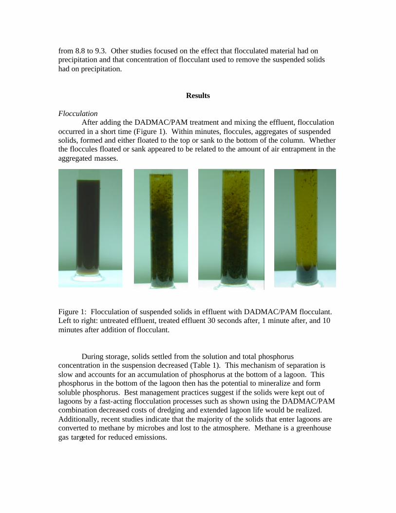
Flocculation After adding the DADMAC/PAM treatment and mixing the effluent, flocculation

occurred in a short time (Figure 1). Within minutes, floccules, aggregates of suspended solids, formed and either floated to the top or sank to the bottom of the column. Whether the floccules floated or sank appeared to be related to the amount of air entrapment in the aggregated masses.

Figure 1: Flocculation of suspended solids in effluent with DADMAC/PAM flocculant. Left to right: untreated effluent, treated effluent 30 seconds after, 1 minute after, and 10 minutes after addition of flocculant.

During storage, solids settled from the solution and total phosphorus concentration in the suspension decreased (Table 1). This mechanism of separation is slow and accounts for an accumulation of phosphorus at the bottom of a lagoon. This phosphorus in the bottom of the lagoon then has the potential to mineralize and form soluble phosphorus. Best management practices suggest if the solids were kept out of lagoons by a fast-acting flocculation processes such as shown using the DADMAC/PAM combination decreased costs of dredging and extended lagoon life would be realized. Additionally, recent studies indicate that the majority of the solids that enter lagoons are converted to methane by microbes and lost to the atmosphere. Methane is a greenhouse gas targeted for reduced emissions.

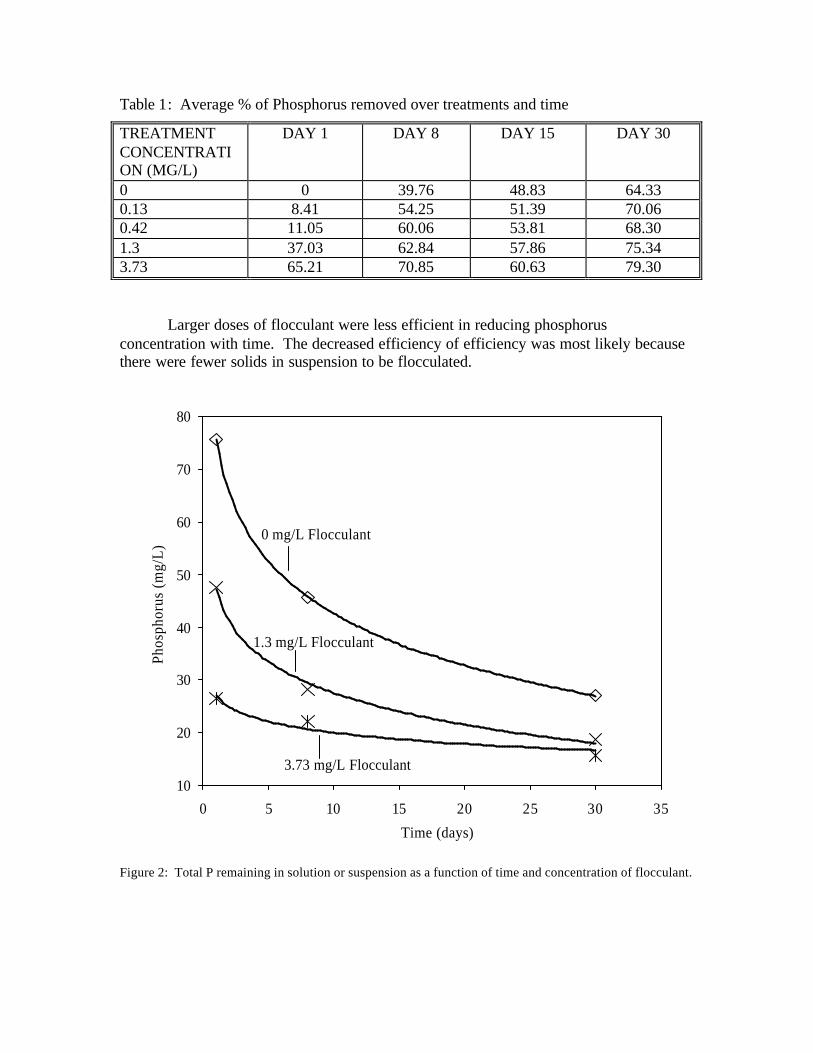
Table 1: Average % of Phosphorus removed over treatments and time

TREATMENT CONCENTRATION (MG/L)

DAY 1 DAY 8 DAY 15 DAY 30

0 0 39.76 48.83 64.33 0.13 8.41 54.25 51.39 70.06 0.42 11.05 60.06 53.81 68.30 1.3 37.03 62.84 57.86 75.34 3.73 65.21 70.85 60.63 79.30

Larger doses of flocculant were less efficient in reducing phosphorus

concentration with time. The decreased efficiency of efficiency was most likely because there were fewer solids in suspension to be flocculated.

0 mg/L Flocculant

1.3 mg/L Flocculant

3.73 mg/L Flocculant10

20

30

40

50

60

70

80

0 5 10 15 20 25 30 35

Time (days)

Phos

phor

us (m

g/L)

Figure 2: Total P remaining in solution or suspension as a function of time and concentration of flocculant.

Precipitation When effluent pH was raised above 9 with addition of NH4OH, soluble

phosphorus and calcium declined considerably (Table 2). The concentrations of magnesium did not show a significant change after the pH was raised so the reduction in phosphorus was probably as one or a combination of numerous possible calcium phosphates compounds. The phosphorus which was removed by raising the pH was not precipitated out as struvite, an ammonium-magnesium phosphate. Struvite forms readily in effluent from swine operations, but not from dairy operations. Table 2: Average Phosphorus and Calcium reduction after raising the pH to 9.1 with NH4OH at 30 days after suspension.

FLOCCULANT

CONC.

P BEFORE

P AFTER CA BEFORE

CA AFTER

mg/L mg/L mg/L % reduction

mg/L mg/L % reduction

0 25 26 0 217 217 0 0.13 27 9 65 250 31 87 0.42 26 7 71 274 29 89 1.3 18 3 81 274 16 94 3.73 16 2 90 260 14 94

Conclusion Phosphorus concentrations in dairy effluent can be reduced considerably by

treating the effluent with flocculates to remove suspended solids and then with a base such as ammonium hydroxide to precipitate soluble phosphates.

Increase Water Use Efficiency: Implementation of LimitedIrrigation for Crop Biotic and Abiotic Stress Management

Basic Information

Title:Increase Water Use Efficiency: Implementation of Limited Irrigation for CropBiotic and Abiotic Stress Management



End Date: 2/1/2003



23rd


Focus Category: Agriculture, Irrigation, Water Use

Descriptors: None


Nyland R. Falkenberg, Giovanni Piccinna

Publication

1. Falkenberg, Nyland. Site Specific Management of Plant Stress Using Infrared Thermometers andAccu-Pulse. 2002 American Society of Agronomy Meeting (ASA), Indianapolis, IN.

2. Falkenberg, Nyland. Remote Sensing for Site Specific Management of Biotic and Abiotic Stress inCotton. 2003 Beltwide Cotton Conference, Nashville, TN.

3. Falkenberg, Nyland. Will be presenting again at the Beltwide Cotton Conference in San Antonio, TXand in Denver, CO at the American Society of Agronomy Meeting for the 2003-04 meetings.

4. Falkenberg, N. R., G. Piccinni, M. K. Owens, and J. T. Cothren. Increased Water UseEfficiency-Limited Irrigation to Manage Crop Stress: A Remote Sensing Study. Texas WaterResources Institute SR 2003-003.

REMOTE SENSING FOR SITE-SPECIFIC MANAGEMENT OF BIOTIC AND ABIOTIC STRESS IN COTTON

Nyland Falkenberg1, Giovanni Piccinni1, M.K. Owens1, and Dr. Tom Cothren2

1Texas Agricultural Research and Extension Center Uvalde, TX

2Texas Agricultural Experiment Station College Station, TX

Abstract

This study evaluated the applicability of remote sensing instrumentation for site-specific management of abiotic and biotic stress on cotton grown under a center pivot. Three different irrigation regimes (100%, 75%, and 50% ETc) were imposed in the cotton field to: 1) monitor canopy temperatures of cotton with infrared thermometers (IRTs) to pinpoint areas of biotic and abiotic stresses, 2) compare aerial infrared photography to IRTs mounted on center pivots to correlate areas of biotic and abiotic stresses, and 3) to relate yield and yield parameters relative to canopy temperatures. Pivot mounted IRTs and IR cameras were able to differentiate water stress between the irrigation regimes. However, only the IR cameras were effectively able to distinguish between biotic (cotton root rot) and abiotic (drought) stresses with the assistance of ground-truthing. Cooler canopy temperatures were reflected in higher lint yields. The 50% ETc regime had significantly higher canopy temperatures, which were reflected in significantly lower lint yields when compared to the 75 and 100% ETc regimes. Deficit irrigation up to 75% ETc had no impact on yield, indicating that for this year water savings were possible without yield depletion. Canopy temperatures were effective in monitoring plant stress during the canopy development.

Introduction In 1993, the Texas Legislature placed water restrictions on the farming industry by limiting growers to a maximum use of 2 acre-foot of water per year in the Edwards Aquifer Region. Since then, maximization of agricultural production efficiency has become a high priority for numerous studies in the Winter Garden Area of Texas. Recent investigations have proposed Site-Specific Management (SSM) as an alternative to address this problem. SSM involves satellite-based remote sensing technology and mapping systems to detect specific areas suffering from stress within a field (i.e. water, insect, and disease stress). Crop canopy temperature has been found to be an effective indicator of plant water stress (Moran, 1994). Coupled with remote sensing technology, this concept allows collection and analysis of temperature data from crops using infrared thermometers (IRTs). IRTs mounted on irrigation systems or operated from aircraft can detect water stress by recording changes in leaf temperature caused by the alteration of the soil-plant water flow continuum (Hatfield and Pinter, 1993; Michels et al., 1999). Therefore, remote sensing equipment and mapping systems provide an excellent potential for producers to grow crops under high water use efficiency, by treating only the areas where treatment is needed (i.e. irrigation).

Objectives The overall objectives of this project are as follow: 1) use remote sensing instrumentation for locating areas showing biotic and abiotic stress signs and/or symptoms in a cotton field, 2) evaluate canopy temperature changes in cotton with the use of IRTs, 3) and assess yield and yield parameters relative to the canopy temperatures.

Materials and Methods The experiment was conducted at the Texas A&M Agricultural Research and Extension Center in Uvalde, Texas. Cotton variety Stoneville 4892B/Round-up Ready was planted in a circle at 50,000 ppa on 40-inch row spacing and grown under a center-pivot LESA (Low Elevation Sprinkler Application) irrigation system. Furrow dikes were placed between beds to increase water capture and minimize run-off. The soil type is a Knippa clay soil (fine-silty, mixed, hyperthermic Aridic Calciustolls) with a pH of 8.1. Three irrigation regimes (100%ETc, 75%ETc, and 50% ETc) were replicated twice in a randomized block design. A 90-degree wedge was divided equally into six 15-degree regimes, which were maintained at the above mentioned (ETc) values. Thirty Exergen (Irt/c.01-T80F/27C) infrared thermometers (IRTs) were mounted at approximately 15- foot spacing along the pivot length to scan the canopy temperature as the pivot moved. The IRTs recorded canopy temperatures every 10 seconds, and average temperature values every 60 seconds, on a 21X Campbell Scientific datalogger. In addition, canopy temperature differences were determined among treatments using a helicopter equipped with a Mikron 7200 LWIR (Long Wave- length Infrared) infrared camera with infrared band of 8-14 microns. Physiological parameters (i.e., leaf water and osmotic potential) were taken from leaves to determine the level of stress imposed by the different irrigation regimes and the presence of disease. Temperature data were statistically analyzed by ANOVA and separated by Fisher’s LSD at α= 0.05. Aerial infrared temperature readings were analyzed by using the program Mikroscan 2.6.

Results and Discussion Environmental conditions for the 2002 cotton season showed that the minimum and maximum temperatures were normal for the area, but excessive rainfall in the month of July prevented the imposition of differential irrigation regimes. Significant differences in canopy temperature were detected in all three irrigation regimes, with a linear increase in canopy temperature resulting from a decrease in plant water availability. Extreme temperatures detected early in crop development were related to the detection of bare soil and moisture availability in the soil by the IRTs. Pivot mounted IRTs were effective in detecting crop canopy temperature differences between the 3 irrigation regimes. Early in the season there were significant differences between all three irrigation regimes; however, at the end of the growing season no significant differences were found between the 100 and 75% ETc regimes. These results are also best explained by yield differences. No significant differences in lint yield were found between the 75% and 100% ETc

regimes. Yield from the 50% regime were significantly less than the 75% and 100% ETc regimes. This yield reduction is associated with increased canopy temperatures of this regime. Yields were 1160 lb/acre, 1420 lb/acre, and 1600 lb/acre for the 50%, 75%, and 100% ETc treatments, respectively. Abiotic and biotic stress can be differentiated better by the Mikron 7200 than the pivot mounted IRTs because of its increased image scanning resolution. The IR camera was able to detect distinct canopy temperature differences between all 3 irrigation regimes. Biotic stress (root rot) was detected by using the camera before symptoms could be detected visually. Pivot mounted IRTs and IR cameras were able to differentiate water stress between the irrigation regimes, but only IR cameras were able to distinguish between abiotic and biotic stress. There was an excellent correlation between canopy temperature and lint yield. Deficit irrigation up to 75% ETc had no impact on yield, indicating that water savings are possible without yield depletion. Also, canopy temperature can be an excellent tool to monitor plant stress.

References

Barnes, E.M., P.J. Pinter, B.A. Kimball, D.J. Hunsaker, G.W. Wall, and R.L. LaMorte. 2000. Precision irrigation management using modeling and remote sensing approaches. In 4th Decennial Nat. Irri. Symposium. 332-337.

Bugbee, B., M. Droter, O. Monje, and B. Tanner. 1998. Evaluation and modification of

commercial infra-red transducers for leaf temperature measurement. advances in space research. 1-10.

Burke, J.J., J. L. Hatfield, and D. F. Wanjura. 1990. A thermal stress index for cotton. Agron. J. 82: 526-530. Ehler, W.I., S.B. Idso, R.D. Jackson, and R.J. Reginato. 1978. Diurnal changes in plant water potential and canopy temperatures of wheat as affected by drought. Agron.

J. 70: 999-1004. Grimes, D.W., H. Yamada, and S.W. Hughs. 1987. Climate-normalized cotton leaf water

potentials for irrigation scheduling. Agri Water Mgmt. 12: 293-304. Hatfield, J.L. 1990. Measuring plant stress with an infrared thermometer. HortScience.

25: 1535-1538. Hatfield, J. L., and P.J. Pinter, Jr. 1993. Remote sensing for crop protection. Crop Prot. 12: 403-413. Humes, K.S., W.P. Kustas, and M.S. Moran, Use of remote sensing and reference site

measurements to estimate instantaneous sur face energy balance components over a semiarid rangeland watershed. Water Resources Research, Vol. 30, No. 5, pp. 1363-1373, 1994.

Isdo, S.B., R.J. Reginato, D.C. Reicosky, and J.L. Hatfield. 1982. Determining soil- induced plant water potential depressions in Alfalfa by means of infrared thermometry. Agronomy Journal. 73: 826-830.

Jeger, M. J. and S.D. Lyda. 1986. Phymatotrichum root rot (Phymatotrichum

omnivorum) in cotton: environmental correlates of final incidence and forecasting criteria. Annals of Applied Biology. 109: 523-534.

Jenkins, J.N., J.C. McCarty, and W.L. Parrott. 1990. Competition between adjacent

fruiting forms in cotton. Crop Sci. 30: 857-860. Kenerley, C.M., and M.J. Jeger. 1990. Root colonization by Phymatotrichum

omnivorum and symptom expression of Phymtotrichum root rot in cotton in relation to planting date, soil temperature and soil water potential. Plant Pathology. 39: 489-500.

Kenerley, C.M., T.L. White, M.J. Jeger, and T.J. Gerik. 1998. Sclerotial formation and

strand growth of Phymatotrichopsis omnivore in minirhizotrons planted with cotton at different soil water potentials. 47: 259-266.

King, C.J., and H.F. Loomis. 1929. Cotton root rot investigations in Arizona. Journal

Agricultural Research. 39: 199-221.

Kustas, W.P., M.S. Moran, K.S. Humes, D.I. Stannard, P.J. Pinter, Jr., L.E. Hipps, E. Swiatek, and D.C. Goodrich, Surface energy balance estimates at local and regional scales using optical remote sensing from an aircraft platform and atmospheric data collected over semiarid rangelands, Water Resources Research, Vol. 30, No. 5, pp. 1241-1259, 1994.

Lyda, S.D., 1978. Ecology of Phymatotrichum omnivorum. Annual Review of

Phytopathology. 16: 193-209. Maas, S.J., G.J. Fitzgerald, W.R. DeTar, and P.J. Pinter Jr. 1999. Detection of water

stress in cotton using Multispectral remote sensing. Proc-Beltwide-Cotton- Conf. 1: 584-585.

Mahrer, Y. 1990. Irrigation Scheduling with an Evapotranspiration Model: A Verification

Study. Acta Hort. (ISHS) 278:491-500 Marani, A., R.B. Hutmacher, and C.J. Phene. 1993. Validation of CALGOS: simulation

of leaf water potential in drip- irrigated cotton. Proc-Beltwide-Cotton-Conf. 3: 1225-1228.

Michels, G.J. Jr., G. Piccinni, C.M. Rush, and D.A. Fritts. 1999. Using infrared transducers to sense greenbug (homoptera: aphididae) infestations in winter

wheat. Southwestern Entomologist. 24: 269-279.

Moran, M.S., Y. Inoune, and E.M. Barnes. 1997. Opportunities and limitations for

image-based remote sensing in precision crop management. Remote Sens. Environ. 61: 319-346.

Nilsson, H.E. 1995. Remote sensing and image analysis in plant pathology. Annual

Review of Phtopathology. 33: 489-527. Plant, R.E., D.S. Munk, B.R. Roberts, R.N. Vargas, R.L. Travis, D.W. Rains, and R.B.

Hutmacher. 2001. Application of Remote Sensing to Strategic Questions in Cotton Management and Research. Journal of Cotton Science. 5: 30-41.

Rogers, C.H. 1942. Cotton root rot studies with special reference to sclerotia, covercrops,

rotations, tillage, seedling rates, soil fungicides, and effects on seed quality. Bulletin 614, Texas Agricultural Experiment Station, 45pp.

Rush, C.M., D.R. Upchurch, and T.J. Gerik. 1984. In situ observations of Phymatotrichum

omnivorum with a boroscope minirhizotron system. Phytopathology. 74: 104-105. Schepers, J.S., and D.D. Francis. 1998. Precision agriculture – what’s in our future. Commun. Soil Sci. Plant Anal. 29: 1463-1469. Streets, R.B., and H.E. Bloss. 1973. Phymatotrichum Root Rot. APS Monograph no. 8.,

St. Paul, Minnesota, USA: American Phytopathological Society. Stewart, R.B., E. I. Mukammal, and J. Wiebe. 1978. The use of thermal imagery in

defining frost prone areas in the Niagra fruit belt. Remote Sens. Environ. 7: 187-202.

Wanjura, D.F., D.R. Upchurch, J.R. Mahan. 1992. Automated irrigation based on

threshold canopy temperature. Trans ASAE. 35: 153-159. Yang, C. and G.L. Anderson. 2000. Mapping grain sorghum yield variability using

airborne digital videography. Precision agriculture. 2: 7-23. Acknowledgements Megan Laffere Cotton Physiology Workgroup at College Station For additional information email: [email protected]

Higher-Order Statisticts in Transport and Evolution of Algae Blooms

Basic Information

Title: Higher-Order Statisticts in Transport and Evolution of Algae Blooms



End Date: 2/1/2003


Congressional District: 10th


Focus Category: Water Quality, Nutrients, Ecology

Descriptors: None

Principal Investigators: Jordan E. Furnans, Ben R. Hodges

Publication

1. Furnans, Jordan, David Maidment, and Ben Hodges. An Integrated Geospatial Database for TotalMaximum Daily Load Modeling of the Lavaca Bay - Matagorda Bay Coastal Area. Texas WaterResources Institute SR 2002-018.

Higher-Order Statistics in Transport and Evolution of Algae Blooms

By Jordan Furnans The purpose of this project was to determine the capacity of numerical models for transporting distributive information needed for accurate modeling of algal blooms. The first phase of this project involved a numerical analysis of the feasibility of modifying the standard transport equation for quantities more accurately described by higher order statistics rather than just by mean values. This numerical exercise demonstrated reasonable results are obtainable as by applying the transport equation to local mean values across the distribution of the quantity transported by the flow. It also demonstrated the need to develop “particle tracking” capabilities in the numerical models in order to accurately describe the energy flux path the particles & transported objects follow in the flow. This path determines the environmental conditions to which the transported substance is subjected, and therefore aides in determining the affects of the conditions on the time history of the transported substance. In reference to algal blooms, the energy flux path is vital in determining the life history of the algae particles contributing to a bloom. The second phase of this project involved the development of sub-grid scale particle tracking capabilities within the 3D hydrodynamic model ELCOM. This work was conducted while I was researching at the University of Western Australia on a US Fulbright Fellowship. The particle tracking model that was developed has been checked for accuracy against field measurements of drifter movement in Lake Kinneret (Israel) as well as in the Marmion Marine Park in Western Australia. Further analysis is being conducted, but the preliminary results are that the particle tracking model follows directly from the results of the hydrodynamic model, and variations between field and numerical drifter results are predominantly indicators of the overall inaccuracy of the hydrodynamic model given the boundary conditions imposed. The third phase of this work will involve the quantification of horizontal dispersion/diffusion coefficients detemined from field and numerical drifters. This work will form the final portion of my Ph.D. research, which will be completed by May, 2004. The papers that are currently under development as a result of the TWRI grant are:

1. On Horizontal Dispersion in the Coastal Boundary Layer 2. Numerical Modeling of Lagrangian Drifters

These working titles are likely to be changed. The first paper focuses on the calculation of horizontal dispersion coefficients in the costal zone using field and numerical drifters in Marmion Marine Park. The second paper details the working numerics and the accuracy of the particle tracking routine within the ELCOM model, as verified against an analytically derived velocity field. Each of these topics will be addressed in the final report submitted to TWRI in June, 2003.

Real-Time Distributed Runoff Estimation Using NEXRADPrecipitation Data

Basic Information

Title: Real-Time Distributed Runoff Estimation Using NEXRAD Precipitation Data



End Date: 2/1/2003




Focus Category: Models, Floods, Hydrology

Descriptors: None

Principal Investigators: Jennifer Hadley, Raghavan Srinivasan

Publication

1. Hadley, Jennifer. Near Real-Time Runoff Estimation Using Spatially Distributed Radar RainfallData. Texas Water Resources Institute SR-2003-015.

The objective of this study is to develop near real-time runoff estimation for Texas using precipitation data from the Next Generation Weather Radar (NEXRAD) network. This will provide information useful for flood mitigation, reservoir operation, and watershed and water resource management practices. Materials and Methods The datasets used in this analysis were the USGS Multi-Resolution Land Characteristic (MRLC) dataset, the USDA-NRCS State Soil Geographic Database (STATSGO), and the Next Generation Weather Radar (NEXRAD) data. The MRLC dataset served as the land cover information and the STATSGO database was used to determine the hydrologic soil group for the analysis areas. Corrected NEXRAD data was used for daily precipitation information. The runoff estimates for each grid cell were calculated using the Soil Conservation Service (SCS) Curve Number Method, which provides a means of estimating runoff based on land uses, soil types, and precipitation. This calculation is based on the retention parameter, S, initial abstractions, Ia (surface storage, interception, and infiltration prior to runoff), and the rainfall depth for the day, Rday, (all in mm H2O). The retention parameter is variable due to changes in soil type, land use, and soil moisture, and is defined as:

S = (1000 / CN-10), where CN is the assigned SCS curve number For the runoff calculations, initial abstractions were approximated as 0.2S, and NEXRAD rainfall maps were used to identify Rday. The runoff equation becomes: Qsurf = (Rday – 0.2S)2 / (Rday + 0.8 S) Runoff will occur only when Rday > Ia (Neitsch et al., 2001). A curve number (CN) grid was generated based on the MRLC and STATSGO datasets at a 100m × 100m resolution with the use of ESRI’s ArcInfo and the ArcGIS 3.1.2 raster calculator. The CN was assigned based on average soil moisture conditions (Table 1), and then altered to account for the antecedent soil moisture conditions. Table 1. Curve number assignments based on land use / land cover

Land Use/ Land Cover Curve Numbers (Soil Hydrologic Group A, B, C, D)

Water 100 Urban 77, 85,90,92 Forest 36, 60, 73, 79

Rangeland 30, 58, 71, 78 Pasture 49, 69, 79, 84

Agriculture 67, 78, 85, 89 Wetland 100

Real-Time Distributed Runoff Estimation Using NEXRAD Precipitation Data Progress Report by

Jennifer Hadley, Forest Science Department, TAMU

2

Figure 1. “True” runoff summary map.

Figure 2. Average runoff summary map.

The antecedent soil moisture conditions were defined as dry (wilting point), average, or wet (field capacity), and were based on the previous five-day rainfall totals (Table 2) (Mitchell et al., 1993). Table 2. Rainfall break points for antecedent soil moisture conditions.

An Arc Macro Language (AML) script and batch file was used with ESRI’s ArcInfo software to make the daily calculations for the study period, April 1 - 15, 2002. First, the rainfall totals for March 27 - 30 were calculated. This information was then used to estimate the antecedent soil moisture conditions for April 1. Through the use of an “if- then” statement, the script then applied the appropriate CN grid to the NEXRAD rainfall data to calculate the “true” runoff for the current day. A batch file was then used to create a semi-automated way of processing the data for each consecutive day in the study period. For comparison purposes, the runoff maps were re-calculated using only average antecedent soil moisture conditions, and summary and difference maps were generated for the two map sets. An additional AML was used to calculate total runoff for the “true” and average runoff datasets (Figures 1& 2). This same AML then subtracted the “true” runoff summary from the average runoff summary to generate a difference map (Figure 3). “True” runoff ranged from 16.29 – 1,706.56 mm, whereas average runoff ranged from 0 – 355.36 mm. The differences between the “true” and average summaries ranged from -40.29 – 1,706.56 mm.

Antecedent Moisture Conditions Rainfall Range

I - Wilting Point < 12 mm

II – Average 12-41 mm

III – Field Capacity > 41 mm

3

Figure 3. Difference map: “true” – average runoff.

Results and Discussions Although the runoff vales estimated in this analysis have not been calibrated they do highlight the potential issues involved in estimating runoff without accounting for the antecedent conditions along with land cover and soil hydrologic group. In general, the “true” runoff was substantially higher than the average values. In some cases however, the average calculations did generate higher runoff, as evidenced by the negative values in the difference map. This could be attributed to the fact that the antecedent soil moisture conditions were generally wetter than average, generating additional runoff when factored into the calculations, or dryer than average in the case of the over-estimated average runoff values. Although the runoff values generated here are not indicative of actual runoff values for Texas, they do illustrate the need for accurately estimating antecedent soil moisture conditions in surface runoff calculations. Future Considerations The results of this analysis need further calibration and validation to determine the appropriate rainfall break-points for various antecedent soil moisture conditions and to evaluate the accuracy of runoff estimates. The process of generating these maps must also be automated to achieve the ultimate goal of the research, which is a daily surface runoff map of Texas at a resolution of 4km × 4km. Once calibration and validation procedures are complete, these runoff maps would be made available on the World Wide Web (WWW) for use by public and private water resource managers and various government agencies. References Cited Mitchell, J.K., B.A. Engel, R. Srinivasan, R.L. Bingner, and S.S.Y. Wang, 1993. Validation of AGNPS for Small Mild Topography Watersheds Using an Integrated AGNPS/GIS. In Advances in Hydro-Science and Engineering, Volume I, ed. S.S.Y.Wang, 503-510. University, MS: Center for Computational Hydroscience and Engineering. Neitsch, S.L., J.G. Arnold, J.R. Kiniry, and J.R. Williams, 2001. Soil and Water Assessment Tool Theoretical Documentation. Blackland Research Center, Texas Agricultural Experiment Station. Temple, Texas. 93-115.

Reduced Phosphorus Concentrations in Feedlot Manure and Runoff

Basic Information

Title: Reduced Phosphorus Concentrations in Feedlot Manure and Runoff



End Date: 2/1/2003




Focus Category: Agriculture, Water Quality, Nutrients

Descriptors: None

Principal Investigators: Kevin Heflin, Brent W. Auvermann

Publication

Reduced Phosphorus Concentrations in Feedlot Manure and Runoff

Progress Report By

Kevin Heflin A beef cattle feeding trial was conducted at the TAES/ USDA-ARS experimental feedyard, at Bushland, Texas. The feeding trial focused on the reduction of phosphorus in the cattle diet to reduce the concentration of phosphorus in the excreted manure. The 188 cattle were fed 4 different diets with varying levels of phosphorus in 18 feed pens from June-December 2002. Each feed pen measured 6m x 27m (162m2). Surfaces for 12 of the feed pens consisted of compacted fly ash, and the remaining 6 pen surfaces were native soil. Water samples were collected from 6 different rain events that produced sufficient runoff from the pen surfaces. Water samples were collected with an ISCO 3700 that was activated automatically by runoff waters. Each sampler is capable of collecting 24 samples with each sample containing 1000 ml. Water samples were collected at 5 minute intervals until all 24 bottles were filled or runoff levels were not sufficient to trigger the sampler. Due to the large volume of water samples (500+) results are still pending.

Fate of a Representative Pharmaceutical in the Environment

Basic Information

Title: Fate of a Representative Pharmaceutical in the Environment



End Date: 2/1/2003




Focus Category: Toxic Substances, Ecology, Non Point Pollution

Descriptors: None

Principal Investigators: audra.morse.1, Andrew Jackson

Publication

1. Morse, Audra and Andrew Jackson. Fate of a representative pharmaceutical in the environment.TexasWater Resources Institute TR-227.

Fate of a representative pharmaceutical in the environment

Final Report

Submitted to

Texas Water Resources Institute

By:

Audra Morse, Ph.D. Andrew Jackson, Ph.D., P.E.

May, 2003

ii

TABLE OF CONTENTS

Abstract iii

List of Tables iv

List of Figures v

INTRODUCTION 1

BACKGROUND 4

Amoxicillin 5

Antibiotics in the Environment 9

Antibiotic Resistance 12

Antibiotic Resistance in WWTP Influent 12

Antibiotic Resistance in WWTPs and Their Discharges 13

WWTP Discharges and Their Effect on the Natural Environment 14

Antibiotic Resistance Transfer 15

Summary 16

Lubbock Water Reclamation Plant 16

EXPERIMENTAL PROCEDURE 19

Fate of Amoxicillin in a Water Reclamation Plant—Lubbock, TX 19

Antibiotic Resistance 19

Disk Diffusion Susceptibility Tests 19

Antibiotic Resistance in the LWRP 20

Media Preparation and Sterilization Procedures 21

Sterilization 22

Amoxicillin Quantification 22

RESULTS AND DISCUSSION 23

Fate of amoxicillin in a Water Reclamation Plant—Lubbock, TX 23

Antibiotic Resistance in the LWRP 24

CONCLUSIONS AND RECOMMENDATIONS 28

BIBLIOGRAPHY 30

APPENDIX 35

iii

ABSTRACT

The purpose of this research was to determine the fate of amoxicillin in the City

of Lubbock’s Water Reclamation Plant and to determine the antibiotic resistance patterns

in the plant. Amoxicillin was detected in the influent of the plant during one month of

the study, but amoxicillin was not detected at any other plant flow streams. The

antibiotic resistance patterns of the LWRP varied monthly; heterotrophic bacteria were

resistant to most of the antibiotics investigated during the nine month study.

iv

LIST OF TABLES

Table 1. Concentrations of selected antibiotics applied in Germany 10 Table 2. Summary of antibiotics in streams in U.S. 11 Table 3. Antibiotics and concentrations of susceptibility disks 20 Table 4. Summary of antibiotics and resistance mechanisms 21 Table 5. Amoxicillin concentrations in the LWRP 23 Table 6. Antibiotic Resistance in the Influent of the LWRP 25 Table 7. Antibiotic Resistance in the Primary Sludge of the LWRP 25 Table 8. Antibiotic Resistance in the Activated Sludge of the LWRP 26 Table 9. Antibiotic Resistance in the Effluent of the LWRP 26 Table A.1. LWRP susceptibility test results for June 36 Table A.2. LWRP susceptibility test results for July 37 Table A.3. LWRP susceptibility test results for August 38 Table A.4. LWRP susceptibility test results for September 39 Table A.5. LWRP susceptibility test results for October 40 Table A.6. LWRP susceptibility test results for November 41 Table A.7. LWRP susceptibility test results for December 42

v

LIST OF FIGURES

Figure 1. Sources, pathways, and sinks of pharmaceuticals 2 Figure 2. Chemical structure of amoxicillin and penicilloic acid 6 Figure 3. Structure of Gram-positive and Gram-negative bacteria 7 Figure 4. Beta- lactamases and their distribution in nature 8 Figure 5. Schematic of the LWRP 18

1

INTRODUCTION

As existing potable water supplies are depleted and populations continue to grow

in arid and semi-arid areas of the country, including West Texas, the need for complete

recycling of wastewater for water distribution may become necessary. Already the

dilution factor for wastewater effluent continues to decrease with shorter and shorter

intervals between release and reuse. Many municipalities are in fact using treated

effluent in their primary water source although it may have spent some time in a natural

water course. Historically, the concern with recycled wastewater has been the presence

of disease-causing organisms called pathogens. However, a more recent concern of

reusing wastewater for consumption is the presence of chemical contaminants, including

a new category of compounds: personal care products and pharmaceuticals.

Pharmaceuticals, including anti- inflammatories, ant ibiotics, caffeine, hormones,

antidepressants, and others have been observed in various water bodies (Ternes et al.,

1998; Heberer et al., 1998; Hirsch et al., 1999; Qiting and Xiheng, 1988).

Antibiotics are one especially troubling class of compounds due to the build-up of

resistance in microbial populations. Antibiotics enter the environment from a variety of

sources including discharges from domestic wastewater treatment plants and

pharmaceutical companies, runoff from animal feeding operations, infiltration from

aquaculture activities, leachate from landfills, and leachate from compost made of animal

manure containing antibiotics (Figure 1). However, antibiotics are not confined to the

natural aquatic environment. Detectable concentrations of antibiotics have been observed

in tap water (Herberer et al., 1998; Masters, 2001). The startling fact is that these

compounds are passing through water treatment processes and contaminating drinking

water supplies. The concentrations of these contaminants typ ically range from

nanogram/liter (ng/L) to microgram/liter (µg/L); the consequences of their presence at

these concentrations are unknown. The overall potential for antibiotic removal by

biological and physiochemical treatment systems and simultaneous risk of antibiotic

resistance development has been relatively unexplored.

2

Figure 1. Sources, pathways, and sinks of pharmaceuticals (Kummerer, 2001).

Research has begun to determine the concentrations of antibiotics in the

environment, and from this information, the health effects to humans and animals may be

estimated by toxicologists. An additional problem that may be created by the presence of

antibiotics at low concentrations in the environment is the development of antibiotic

resistant bacteria. In recent years, the incidence of antibiotic resistant bacteria has

increased and many people believe the increase is due to the use of antibiotics (Walter

and Vennes, 1985). The presence of antibiotics can result in selective pressure that

favors organisms that possess genes coding for antibiotic resistance. This may pose a

serious threat to public health in that more and more infections may no longer be

treatable with known antibiotics (Hirsch et al., 1999). In the event that antibiotic

resistance is spread from nonpathogenic to pathogenic bacteria, epidemics may result. In

fact, bacteria have been observed to transfer their resistance in laboratory settings as well

as the natural environment (Kanay, 1983).

3

The objective of this research was to investiga te the effect of a representative

pharmaceutical in a biological water reclamation system. The antibiotic evaluated in this

study was amoxicillin, which is a semi-synthetic, beta- lactam antibiotic used for a variety

of infections. The focus of this particular project is to determine the fate of amoxicillin in

the City of Lubbock’s Wastewater Reclamation Plant and to determine the antibiotic

resistance patterns in the plant.

4

BACKGROUND

Pharmaceuticals are used in large quantities in human and veterinary medicine or

as food additives in animal production (Stan and Heberer, 1997). In animal feeding

operations, antibiotics are often prescribed as a preventative measure to keep the animals

healthy. The abuse of antibiotics has been rampant since Fleming’s discovery of

penicillin. Antibiotics were prescribed for the treatment of many illnesses and at doses

that may have been inappropriate. There are many forms of antibiotic misuse and abuse.

For instance, viral illnesses should not be treated with antibiotics. Also, patients should

be educated on compliance issues and the importance of proper use of the antibiotic.

Misuse, which includes not completing the prescription, can lead to resistance

development (Leiker, 2000a). Preventative measures that may be taken by a clinician to

reduce antibiotic resistance development include using the most appropriate spectrum

antibiotic for each infection, shortening the duration of antibiotic treatment, knowing

local resistance patterns, and limiting antimicrobial prophylaxis if possible (Leiker,

2000a).

Due to the overuse of antibiotics, bacteria have developed resistances to

antibiotics. There are three main modes of antibiotic resistance that generally render the

antibiotic ineffective, but not all bacteria use the same resistance mechanisms. The first

mechanism prevents the antibiotic from binding with and entering the organism, which

has been observed in some P. aeruginosa (Leiker, 2000b); this form of resistance is

related to Multi-Drug Efflux. Other examples are Steptococcus pnuemoniae and Group A

Streptococci penicillin-resistant mutants that have been isolated in the laboratory due to

immense and common selective pressure; these mutants contain altered penicillin-binding

proteins (Tomasz and Munoz, 1995). The second type of resistance mechanism is the

production of an enzyme that inactivates the antibiotic. The classic example of this

resistance mechanism is the production of beta-lactamase enzymes in H. influenze and M.

catarrhalis, which destroys the beta- lactam ring of the beta- lactam antibiotic. There are

many different enzymes produced by bacteria that are capable of degrading the beta-

lactam ring. Fortunately for bacteria, this type of resistance may be spread to other

bacteria through a process called “transference” (Leiker, 2000b). The last form of

bacterial resistance is the change in the internal binding site of the antibiotic. For

5

example, the site to which the antibiotic binds has been altered so that the antibiotic may

no longer bind, which makes the bacteria are resistant to the antibiotic. This process has

been observed in penicillin- resistant S. pneumoniae.

Antibiotic resistance may spread using various mechanisms, including

conjugation, transduction, and transformation. In conjugation, DNA may be transferred

from one bacterial cell to another in the form of a plasmid. Plasmids may carry genetic

information in addition to the information contained on a chromosome, which bacteria

may use under special conditions. For instance, plasmids may carry the genetic

information for antibiotic resistance, virulence, bacteriocins, and metabolic activity

(Madigan et al., 2000). Transduction is the process in which a part of a donor

chromosome is packaged into a phage head and transferred by viruses. If the virus

packaging mechanism selects genes that confer antibiotic resistance, then resistance may

be spread to bacterial cells infected by the viruses. Transformation is the process in

which cells take up free DNA from the environment (Snyder and Champness, 1997). If

the DNA contains antibiotic resistance genes, then antibiotic resistance may be conferred

to the transformant. Thus the transformant now has the genetic material encoding

antibiotic resistance.

Amoxicillin

Amoxicillin is an orally absorbed broad-spectrum antibiotic with a variety of

clinical uses including ear, nose, and throat infections and lower respiratory tract

infections. As a chemical modification of ampicillin, which is poorly absorbed after oral

administration, amoxicillin is better absorbed by the gastrointestinal tract than ampicillin

(Sum et al., 1989). Amoxicillin is prescribed for the treatment of infections of beta-

lactamase-negative stains, which are bacterial strains that do not possess the ability to

produce beta- lactamase enzymes. Figure 2 presents the chemical structures of

amoxicillin (R=0H) and penicilloic acid, a transformation product produced during beta-

lactam ring cleavage.

6

Figure 2. Chemical structure of amoxicillin (left) and penicilloic acid (right)

(Connor et al., 1994).

Amoxicillin is a semi-synthetic penicillin obtaining its antimicrobial properties

from the presence of a beta- lactam ring. Amoxicillin and other penicillin- like antibiotics

target bacterial cell walls. Beta- lactam antibiotics bind to and inhibit the enzymes needed

for the synthesis of peptidoglycan, a component of bacterial cell walls. As bacteria

multiply and divide, the defective walls cannot protect the organism from bursting in

hypotonic environments and cell death occurs.

Many mechanisms exist for resistance to beta-lactam antibiotics. Resistance is

considered an increase in the minimal inhibitory concentration (MIC) of the antibiotic,

which could be the result of many different mechanisms, whereas tolerance does not alter

the bacteria's susceptibility to the drug but improves bacterial survival during treatment.

For optimal bactericidal action, the dose must be greater than the organism's MIC. In the

case of beta-lactam antibiotics, this dose is approximately four to five times the MIC.

When antibiotic concentration is less then the MIC, bacteria recover from the exposure

and begin growth (Ronchera, 2001). When the drug is prescribed to a patient with the

infection, the dose will be greater than the MIC. However, it is unlikely that wastewater

containing urine and feces will have antibiotic concentrations greater than the MIC;

therefore, antimicrobial effects will probably not be observed. However, low

concentrations of antibiotics encourage the development of antibiotic resistance. Thus,

wastewater streams containing urine and feces likely aid in the development of antibiotic

resistance. In S. aureus, which is a major human pathogen, three mechanisms of beta-

7

lactam resistance have been identified: (1) beta- lactamase-mediation inactivated through

hydrolysis of the beta- lactam nucleus, (2) penicillin-binding proteins (PBP)-associate

intrinsic resistance due to the lower of the affinity of PBPs or the acquisition of new

PBPs, and (3) tolerance of the beta-lactam antibiotic as a result of autolysins inhibition

(Georgepapadakou et al.,1988). PBPs are the enzymatic targets of beta-lactam

antibiotics. Beta- lactam resistance due to the alteration of PBPs has been detected in

many isolates as well as most of the major human invasive pathogens (Tomasz, 1988).

For Gram-negative organisms, such as E. coli and nitrifying organisms, another

mechanism of resistance to beta- lactam antibiotics, including amoxicillin, is the hindering

of diffusion of the antibiotic by the outer membrane, which acts as a permeability barrier

(Frere and Joris, 1988). Antibiotics must pass through porins, which are non specific

outer membrane channels. The antibiotics ability to pass through porins depends on the

size, hydrophobicity, and charge of the antibiotic (Danziger and Pendland, 1995). In

addition, the outer membrane prevents the leaking of beta- lactamases into the culture

environment (Frere and Joris, 1988). All bacteria may be divided into Gram-positive and

Gram-negative organisms. The classification was developed by Gram, which is based on

a dye procedure; the color of the dyed bacteria is related to the composition of bacterial

cell walls. Gram-positive organisms appear blue following a Gram stain, and they posses

a thick layer of peptidoglycan and no outer membrane. Beta- lactam antibiotics easily

penetrate the thick layer of peptidoglycan in Gram-positive bacteria (Danziger and

Pendland, 1995). Gram-negative organisms have an outer membrane and a thin layer of

peptidoglycan inside the periplasmic space and are stained red in a Gram stain. Figure 3

is a drawing of the cell wall structures of Gram-negative and Gram-positive bacteria.

Figure 3. Structure of Gram-positive and Gram-negative bacteria (Madigan et al., 2000).

8

As mentioned previously, beta-lactamases are enzymes that cleave the beta-

lactam ring and render the antibiotic useless. The genetic information for beta-

lactamases is contained on either plasmids or chromosomes; however, genes for

resistance are usually carried by plasmids. Beta-lactamase production may be either

constitutive or inducible. Constitutive production results in a constant level of beta-

lactamase production, which is independent of exposure to antibiotics. If beta- lactamase

production is inducible, then beta- lactamases are produced following exposure to a

signal, such as a beta-lactam antibiotic. Furthermore, production of the beta- lactamases

ceases when the bacterium is no longer exposed to the signal (Danziger and Pendland,

1995). Beta-lactamases are classified according to (1) their genetic location

(chromosome vs. plasmid), (2) gene expression (inducible vs. constitutive), (3)

microorganism, (4) inhibition by beta-lactamase inhibitors, and (5) substrate. Figure 4

presents beta- lactamases and their distribution in nature.

Figure 4. Beta- lactamases and their distribution in nature (Danziger and Pendland,

1995).

9

To reduce the potential for beta- lactam cleavage, beta- lactamase inhibitors are

frequently combined with beta- lactam antibiotics. The purpose of the beta- lactamase

inhibitors is to prevent the beta- lactamases from inactivating the antibiotic thereby

increasing the effectiveness of the antibiotic. Examples of beta- lactamase inhibitors are

sulbactam, clavulanate, and tazobactam (Danziger and Pendland, 1995). In many cases,

amoxicillin is combined with clavulanic acid, a beta- lactamase inhibitor.

Antibiotics in the Environment

Drug residues, including antibiotics, have been observed in various aquatic

environments including groundwater, surface water, and tap water (Alvero, 1987;

Campeau et al., 1996). Sources of antibiotics include the treatment of human infections,

veterinary use (e.g., animal feeding operations), aquaculture, and land application of

compost containing sludge from wastewater treatment plants. In human uses, which will

be the primary focus of this paper, antibiotics enter waste streams through feces and

urine. To demonstrate, Hoeverstadt et al. (1986) detected several antibiotics in human

feces, including trimethoprim and doxycycline in concentrations ranging from 3 to 40

mg/kg and erythromycin concentrations from 200 to 300 mg/kg. The concentration of

antibiotics in urine is dependent on dosage, type of dosing (intravenous, intramuscular, or

oral), food and beverage consumption, and elapsed time since dosage (Mastrandrea et al.,

1984). In addition, absorption is also a property of the antibiotics. For example,

amoxicillin is a chemically modified form of ampicillin and the modifications improve its

absorption characteristics.

Extreme difficulties arise in estimating the mass of antibiotics entering the

environment. In general, records containing the quantity of antibiotics prescribed

annually are incomplete and the data available varies from country to country.

Furthermore, it is unknown if the medication is taken as prescribed. Absorption rates

vary for each individual further complicating the estimate of antibiotics entering the

environment. Therefore, researchers have begun analyzing environmental samples for

the presence of antibiotics. Table 1 presents the concentration of antibiotics present in

secondary effluent and surface water in Germany.

10

Table 1. Concentrations of selected antibiotics applied in Germany (Zwiener et al.,

2001).

Antibiotic

Prescribed Mass

(tons/yr)

Secondary Effluent

Concentration (µg/L)

Surface Water

Concentration (µg/L)

Clarithromycin 1.3-2.6 0.24 0.26

Erythromycin 3.9-19.8 6.00 1.70

Roxithromycin 3.1-6.2 1.00 0.56

Chloramphenicol -- 0.56 0.06

Sulfamethoxazole 16.6-76 2.00 0.48

Trimethoprim 3.3-15 0.66 0.20

In the United States, the U.S. Geological Survey completed a study that measured

the concentrations of 95 organic wastewater contaminant s (OWCs) in water samples

from 139 streams in thirty states during 1999 and 2000 (Kolpin et al., 2002). OWCs

include pharmaceuticals, hormones, and other organic contaminants. The compounds

detected represented a wide range of residential, industrial, and agricultural sources. The

most frequently detected compounds were coprostanol (fecal steroid), cholesterol (animal

and plant steroid), insect repellant (N,N-diethyltoluamide), caffeine, triclosan

(antimicrobial disinfectant), fire retardant (tri(2-chloroethyl)phosphate), and a nonionic

detergent metabolite (4-nonylphenol). In addition to these compounds, 31 veterinary and

human antibiotic and antibiotic metabolites were investigated. Fourteen of the 31

antibiotics were not detected in this study. Table 2 contains the antibiotic, frequency of

detection, maximum detected concentration (µg/L), and median detected (µg/L)

concentration of the remaining 17 antibiotics.

11

Table 2. Summary of antibiotics in streams of the U.S. (Kolpin et al., 2002).

Antibiotic

Number of

Samples

Reporting

Level (µg/L)

Frequency

(%)

Max

(µg/L)

Median

(µg/L)

Chlortetracycline (1) 84 0.10 2.4 0.69 0.42

Ciprofloxacin 115 0.02 2.6 0.03 0.02

Erythromycin-H20 104 0.05 21.5 1.7 1.0

Lincomycin 104 0.05 19.2 0.73 0.06

Norfloxacin 115 0.02 0.9 0.12 0.12

Oxytetracycline (2) 84 0.10 1.2 0.34 0.34

Roxithromycin 104 0.03 4.8 0.18 0.05

Sulfadimethozine (2) 84 0.05 1.2 0.06 0.06

Sulfamethazine (1) 104 0.05 4.8 0.12 0.02

Sulfamethazine (2) 84 0.05 1.2 0.22 0.22

Sulfamethizole (1) 104 0.05 1.0 0.13 0.13

Sulfamethoxazole (1) 104 0.05 12.5 1.9 0.15

Sulfamethoxazole (3) 84 0.023 19 0.52 0.066

Tetracycline (2) 84 0.10 1.2 0.11 0.11

Trimethoprim (1) 104 0.03 12.5 0.71 0.15

Trimethoprim (3) 84 0.014 27.4 0.30 0.013

Tylosin (1) 104 0.05 13.5 0.28 0.04

Several studies have identified antibiotics in wastewater treatment plant (WWTP)

flow streams and in WWTP effluents (Stelzer et al., 1985; Grabow et al., 1976; Bell,

1979; Misra et al., 1979; Radtke and Gist, 1989; Malik and Ahmad, 1994) at

concentrations from ng/L to µg/L. Alder et al. (2000) detected up to 0.8 µg/L of

cirpofloxacin in a WWTP effluent and 0.01 to 0.29 µg/L in the WWTP influent. Hirsch

12

et al. (1999) found erythromycin concentrations up to 6 µg/L in WWTP effluent.

Ciprofloxacin was observed in hospital effluent at concentrations between 3 and 89 µg/L,

which is significantly higher than concentrations presented in other studies. Amoxicillin

concentrations in wastewater from a German hospital were between 28 and 82.7 µg/L

(Henninger et al., 2000). Peniciloly groups were observed at concentrations greater than

25 ng/L and 10 µg/L in river water and potable water, respectively (Halling-Sorensen et

al., 1998). Therefore, wastewater treatment plants (WWTPs) are receiving wastes that

contain low concentrations of antibiotics. Exposure to small concentrations of antibiotics

selects for organisms resistant to antibiotics. Subsequently, WWTPs may be a reservoir

of antibiotics as well as antibiotic resistant bacteria.

Antibiotic Resistance

Antibiotic resistance has been observed in various aquatic environments including

river and costal areas, domestic sewage, surface water and sediments, lakes, sewage

polluted ocean water, and drinking water (Merzioui and Baleux, 1994). These aquatic

environments represent a variety of ecosystems and may include a variety of climates.

The consequences of antibiotic resistant organisms may be different for each

environment.

WWTPs are used to treat domestic and industrial wastewater so that it may be

disposed in the natural aquatic environment, including rivers, lakes and streams, with

minimal impact on aquatic life. Currently, the WWTP effluent must meet regulatory

limits for suspended solids, nutrients, fecal coliforms, total coliforms, and a biological

oxygen demand; however, regulatory limits have not been developed for antibiotic agents

and the effect of low antibiotic concentrations and antibiotic resistance development

receives limited attention. The role of WWTPs on the spread of antibiotic resistance to

the natural environment is an important key to the ecological impact of human

discharges.

Antibiotic Resistance in WWTP Influent

WWTPs typically accept discharges from hospitals and may receive discharges

from pharmaceutical plants. Guardabassi et al. (1998) investigated the antibiotic

13

resistance of Acintobacter spp. in sewers receiving waste from a hospital and

pharmaceutical plant. The level of susceptibility to six antimicrobial agents was

determined in 385 Acinetobacter strains isolated from samples collected upstream and

downstream from the hospital and pharmaceutical plant. The antimicrobial agents

analyzed include amoxicillin, oxytetracycline, chloramphenicol, sulfamethoxazole,

gentamicin, and ciprofloxacin. A prevalence of oxytetracycline resistance was observed

to increase in the sewer as the result of hospital discharge; however, the level of

resistance decreased downstream of the discharge.

Antibiotic Resistance in WWTPs and Their Discharges

The incidence of outbreaks involving waterborne antibiotic-resistant bacteria has

led to a serious problem of the death of patients who do not respond to antibiotics. One

source of antibiotic-resistant bacteria in the environment is effluent from WWTPs

(Hassani et al., 1992). The purpose of the Hassani et al. (1992) study was to evaluate the

distribution of Aeromonas species present in wastewater treatment ponds to determine the

effect of treatment on drug resistance incurred by the species. The importance of

evaluating Aeromonas species is that they are a broad group of organisms commonly

found in aquatic environments. During the course of this 17-month study, the

distribution of the Aeromonas observed in the system differed between the cold and

warm months. The most common species of Aeromonas observed were A. caviae, A.

hydrophila, and A. sobria. Seven antibiotics (amoxicillin, cephalothin, streptomycin,

trimethoprim-sulfamethoxazole, chloramphenicol, polymyxin B, and nalidixic acid) were

tested on 264 isolates in this study. All of the isolates were resistant to amoxicillin and

73 percent exhibited resistance to cephalothin, both of which are beta- lactam antibiotics.

The overall frequency of multiple antibiotic resistances among bacterial isolates was 77

percent and the antibiotic resistance index for the total strains was 0.29. Temperature

appeared to have an effect on multiple-drug resistance. During the warm months, the

level of resistance was greater in the bacteria isolated from the influent than those

isolated in the effluent from the pond. Overall, the A. sobria were more susceptible to the

antibiotics investigated in this study than either A. caviae or A. hydrophila. In addition,

each species exhibited different resistance patterns than the other species. For example,

14

the resistance to cephalothin of A. caviae, A. hydrophila and A. sobria were 91, 96 and 9

percent, respectively.

Another study evaluated the effect of wastewater stabilization ponds on antibiotic

resistance on Aeromonas (Imzilin et al., 1996). Differences in resistance patterns of

Aeromonas isolated from the raw sewage and stabilization pond effluent were not

observed. All strains possessed multiple resistances, including resistance to ampicillin,

amoxicillin, and novobiocin. Approximately 90 percent of the strains of A. hydrophila

and A. caviae were resistant to cephalothin, and almost 80 percent of the A. sobria were

susceptible. The results of this study are fairly similar to the results obtained from the

study by Hassani et al. (1992).

Mezriou and Baleux (1994) investigated the antibiotic resistance of 879 E. coli

strains isolated from raw domestic sewage and the effluent from aerobic lagoons and

activated sludge plants. Both aerobic lagoons and activated sludge plants are used to

reduce the BOD5 leaving the treatment facility. The results of this study indicate that the

aerobic lagoons were effective in removing fecal coliforms in the wastewater, but the

system selected for antibiotic resistant E. coli by selecting for E. coli. The number of

antibiotic resistant strains of E. coli in the effluent increased as compared to the influent.

For both the inflow and outflow, the incidence of antibiotic resistance increased as the

number of antibiotics was reduced from seven to one. The maximum polyresistance for a

strain was seven antibiotics (ampicillin, mezlocillin, gentamicin, netilmicin, tobramycin,

doxycyclin, and chloramphenicol). The level of antibiotic resistant E. coli strains in the

outflow of the activated sludge was not constant and did not appear to develop in a

manner similar to the aerated lagoon. In both the activated sludge and aerated lagoon

system, resistance to quinolones and aminosides was not observed.

WWTP Discharges and Their Effect on the Natural Environment

To evaluate the impact of urban effluent, including WWTP discharges, Goni-

Urriza et al. (2000) investigated antibiotic resistance in bacteria isolated from the Arga

River in Spain. River samples were collected upstream and downstream of the water

discharged from the city of Pamplona’s WWTP. Enterobacteriaceae, from human and

animal commensal flora, and Aeromonas were investigated. Most Aeromonas (72

15

percent) and 20 percent of the Enterobacteriaceae were resistant to nalidixic acid, which

is a quinolone. The rate at which antibiotic resistances decreased downstream from the

discharge was similar for the two groups of bacteria. Genetic analysis indicated that

these resistances were mostly chromosomal mediated for Enterobacteriaceae and

exclusively chromosomally mediated for Aeromonas. Other studies have observed less

resistance of native and fecal bacteria upstream of urban areas and WWTP discharges,

increased resistance immediately downstream of urban areas and WWTP discharges, and

decreased resistance farther downstream (Boon and Cattanach, 1999; Pathak et al., 1993;

Iwane et al., 2001). Another study by Gonzalo et al. (1989) evaluated antibiotic

resistance and virulence factors of 418 E. coli strains isolated from river water receiving

sewage discharge. The data indicated that bacteria from less contaminated water present

less antibiotic resistance and virulence factors than those isolated from highly

contaminated water. The results suggest that antibiotic resistance and virulence factors

do not survive well in environments without selective pressure.

Natural aquatic environments, including lakes, rivers, and streams are

environments in which antibiotic resistance may be developed. Arvanitdou et al. (1997)

investigated the transfer of antibiotic resistance among Salmonella strains isolated from

surface waters in northern Greece. Differences in antibiotic use and climate conditions

resulted in geographic variations of antibiotic resistance among bacteria in surface water.

The study showed that 24 percent of the Salmonella strains tested showed resistance to

one or more of the antibiotics tested. Resistance to streptomycin was most common but

was not transferable in all cases. However, ampicillin resistance (ampicillin is a beta-

lactam antibiotic) was transferable. The authors believed these findings supported the

presence of a common plasmid-mediated TEM type beta- lactamase. In one case,

ampicillin resistance was cotransferred with resistance to aminoglycosides. Bacteria of

non-fecal origin in natural aquatic environments free of natural anthropogenic influence

demonstrated antibiotic resistance to one or more antibiotics; resistance may not be

plasmid-mediated (Magee and Quinn, 1991).

Antibiotic Resistance Transfer

16

One of the greatest concerns of antibiotic resistance is the spread of antibiotic

resistance from one bacterial species to another, especially in the case of resistance

transfer between nonpathogenic to pathogenic bacteria. Antibiotic resistance has been a

concern in an institutionalized environment such as a hospital; however, it may also be a

concern in aquatic environments such as wastewater treatment systems. Resistance to

newer beta- lactam agents was observed between Klebsiella pneumoniae and E. coli in a

hospital in France, as observed by a decreased susceptibility of E. coli to cefotaxime.

Three beta- lactamases were identified mediating cefotaxime resistance as well as

penicllin and other cephalosporin resistance. Therefore, these beta-lactamases were

termed extended broad-spectrum beta- lactamases (Jarlier et al., 1988).

Evidence suggests that healthy members of a community may contain a reservoir

of bacterial antibiotic resistance genes even in commensal flora (Shanahan et al., 1994).

These resistance reservoirs may complicate treatment of infections by invading pathogens

who transfer resistance to nonpathogens. In Gram-negative bacteria, resistance is

commonly mediated by TEM-1 beta- lactamases, which have been shown to account for

up to 80 percent of all plasmid-mediated resistance. In Edinburgh, U.K., antibio tic

resistance was observed in healthy human subjects, including resistance to ampicillin.

Plasmids containing TEM-1 beta- lactamases encoding information were present

throughout the community and were believed to be culprit of many extended-spectrum

beta-lactamases.

Summary

These studies indicate that industrial and domestic discharges may affect the

antibiotic resistance patterns observed in a WWTP. Furthermore, WWTPs have the

ability to alter the antibiotic resistance patterns of bacteria in ecosystems containing the

WWTP outfall. As a consequence, environmental bacteria, pathogens, and non-

pathogens may confer resistance to currently prescribed antibiotics.

Lubbock Water Reclamation Plant

The Lubbock Water Reclamation Plant (LWRP), located in Lubbock, Texas,

served as the test facility for the fate of amoxicillin in a full-scale wastewater treatment

17

plant. The flow rate for the LWRP is approximately 20 MGD. Figure 5 is a flow

diagram of the LWRP. Note that there are three process streams for the plant, which

have been the result of plant expansions over the many years of operation. Primary

treatment of the influent to the plant consists of screening and grit removal. After

primary treatment, the flow streams are split before secondary treatment. For secondary

biological treatment, the plant employs activated sludge in Plants 3 and 4. Plant 2 uses

biotowers for secondary treatment. The facility does not employ tertiary removal.

Instead, the effluent is used to irrigate farmland, discharged to Yellow House Canyon, or

sent to XCEL. Sludge from secondary treatment is thickened, digested in anaerobic

digesters, dewatered and landfilled.

The fate of amoxicillin in the LWRP was determined by measuring the ambient

concentrations of amoxicillin at four locations in the plant over nine months. The

objective of this experiment is to investigate the fate of amoxicillin in a full-scale

wastewater treatment plant. Due to the dilution of urine by other wastewater streams

entering a full-scale wastewater treatment plant as well as biotic activity in sewer

systems, amoxicillin concentrations were expected to be near the detection limit in the

influent and effluent of the plant, respectively.

18

Figure 5. Schematic of the LWRP.

Lift Station

Bar Screens

Grit Chamber

Plant 2 Plant 3 Plant 4

Primary Clarifiers

Biotowers

Influent

Secondary Clarifiers

Primary Clarifiers

Aeration Basin


Primary Clarifiers

Aeration Basin


EP1

LLAS HLAS

XCEL

EP2

HLAS Stream Discharge

Chlorine Contact

Filters

Cl2 Cl2 Cl2

19

EXPERIMENTAL PROCEDURE

Fate of Amoxicillin in a Water Reclamation Plant--Lubbock, TX

Wastewater samples were collected from the influent, primary sludge, activated

sludge basin, and the effluent of the Plant 4 of the LWRP. Samples were collected by

LWRP personnel on the second Friday of each month from May to December. Samples

were taken immediately to the ESL and filtered using a 0.45 µm filter. The primary

sludge samples were centrifuged before filtering. The wastewater samples were filtered

to prevent clogging of the C18 cartridges, which were required by the amoxicillin

preparation procedure. All amoxicillin wastewater samples were analyzed in triplicate.

Antibiotic Resistance

The change in antibiotic resistance in the LWRP was investigated at four

locations in the plant over eight months. To investigate the occurrence of antibiotic

resistance in microorganisms in the systems examined in this research the disk diffusion

susceptibility test was performed on samples obtained from the systems.

To investigate antibiotic resistance of the bacteria used in LWRP, samples were

collected from the influent, activated sludge tank, primary sludge and effluent. Samples

were collected, by LWRP personnel on the second Friday of each month from May to

December in sterile, 1-L bottles. The samples were immediately taken to the ESL and

analyzed.

The disk diffusion susceptibility test was performed to determine if heterotrophic

organisms in the LWRP samples were resistant to multiple antibiotics. The LWRP

samples were plated on nutrient agar and Hinton-Mueller plates. The antibiotics

investigated in this study include amoxicillin with clavulanic acid and three other beta

lactam antibiotics: penicillin, ampicillin, and cephalothin. Other antibiotics investigated

in this study were bacitracin, ciprofloxacin, rifampin, streptomycin, tetracycline, and

vancomycin. Table 3 lists the antibiotics and their concentrations used in this study.

Table 4 presents a summary of the antibiotics investigated and their mechanisms.

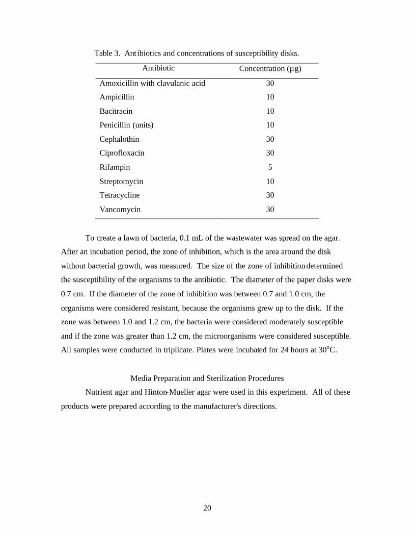
20

Table 3. Ant ibiotics and concentrations of susceptibility disks.

Antibiotic Concentration (µg)

Amoxicillin with clavulanic acid 30

Ampicillin 10

Bacitracin 10

Penicillin (units) 10

Cephalothin 30

Ciprofloxacin 30

Rifampin 5

Streptomycin 10

Tetracycline 30

Vancomycin 30

To create a lawn of bacteria, 0.1 mL of the wastewater was spread on the agar.

After an incubation period, the zone of inhibition, which is the area around the disk

without bacterial growth, was measured. The size of the zone of inhibition determined

the susceptibility of the organisms to the antibiotic. The diameter of the paper disks were

0.7 cm. If the diameter of the zone of inhibition was between 0.7 and 1.0 cm, the

organisms were considered resistant, because the organisms grew up to the disk. If the

zone was between 1.0 and 1.2 cm, the bacteria were considered moderately susceptible

and if the zone was greater than 1.2 cm, the microorganisms were considered susceptible.

All samples were conducted in triplicate. Plates were incubated for 24 hours at 30oC.

Media Preparation and Sterilization Procedures

Nutrient agar and Hinton-Mueller agar were used in this experiment. All of these

products were prepared according to the manufacturer's directions.

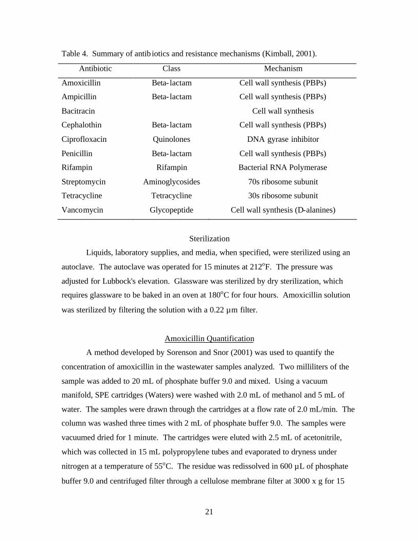
21

Table 4. Summary of antib iotics and resistance mechanisms (Kimball, 2001).

Antibiotic Class Mechanism

Amoxicillin Beta- lactam Cell wall synthesis (PBPs)

Ampicillin Beta- lactam Cell wall synthesis (PBPs)

Bacitracin Cell wall synthesis

Cephalothin Beta- lactam Cell wall synthesis (PBPs)

Ciprofloxacin Quinolones DNA gyrase inhibitor

Penicillin Beta- lactam Cell wall synthesis (PBPs)

Rifampin Rifampin Bacterial RNA Polymerase

Streptomycin Aminoglycosides 70s ribosome subunit

Tetracycline Tetracycline 30s ribosome subunit

Vancomycin Glycopeptide Cell wall synthesis (D-alanines)

Sterilization

Liquids, laboratory supplies, and media, when specified, were sterilized using an

autoclave. The autoclave was operated for 15 minutes at 212oF. The pressure was

adjusted for Lubbock's elevation. Glassware was sterilized by dry sterilization, which

requires glassware to be baked in an oven at 180oC for four hours. Amoxicillin solution

was sterilized by filtering the solution with a 0.22 µm filter.

Amoxicillin Quantification

A method developed by Sorenson and Snor (2001) was used to quantify the

concentration of amoxicillin in the wastewater samples analyzed. Two milliliters of the

sample was added to 20 mL of phosphate buffer 9.0 and mixed. Using a vacuum

manifold, SPE cartridges (Waters) were washed with 2.0 mL of methanol and 5 mL of

water. The samples were drawn through the cartridges at a flow rate of 2.0 mL/min. The

column was washed three times with 2 mL of phosphate buffer 9.0. The samples were

vacuumed dried for 1 minute. The cartridges were eluted with 2.5 mL of acetonitrile,

which was collected in 15 mL polypropylene tubes and evaporated to dryness under

nitrogen at a temperature of 55oC. The residue was redissolved in 600 µL of phosphate

buffer 9.0 and centrifuged filter through a cellulose membrane filter at 3000 x g for 15

22

minutes. Then, 500 µL of the filtrate was transferred to a 15 mL polypropylene tube.

Next, 75 µL of derivitization reagent I was added and the sample was vortex-mixed for

30 seconds. After 10 minutes, 450 µL of derivitization reagent II was added and the

sample was vortex-mixed for 60 seconds. The samples were placed in a water bath

(55oC) to react for 30 minutes. The samples were cooled in cool water and transferred to

vials. The samples were quantified using an HPLC. The injection volume was 500 µL

and the mobile phase flow-rate was 1.0 mL/min. The detection wavelength was 323 nm.

The analytical instrument was calibrated on each day of analysis, and QC samples were

run at a maximum of 20 samples, followed by blanks, to ensure that the instrument was

still calibrated correctly.

23

RESULTS AND DISCUSSION

Fate of Amoxicillin in a Water Reclamation Plant--Lubbock, TX

To investigate the concent ration of amoxicillin in a full-scale wastewater

treatment plant, wastewater samples were collected from the Lubbock Wastewater

Reclamation Plant (LWRP) in Lubbock, Texas. Samples were collected on the second

Friday of every month between May and December 2002. The samples were

immediately taken to the ESL and analyzed for amoxicillin and antibiotic resistance. All

samples were analyzed in triplicate. The purpose of this experiment was to monitor the

fate of amoxicillin in the LWRP to determine if amoxicillin was present in the plant’s

influent and effluent.

During the eight-month experiment, amoxicillin was detected in the influent of

the plant only in the May samples; amoxicillin was not detected at any other sample

locations during any of the months of this study. Table 5 presents a summary of the

amoxicillin analysis. NA indicates not applicable. Due to equipment problems, samples

could not be analyzed in December.

Table 5. Amoxicillin concentrations in the LWRP.

Amoxicillin Concentration (mg/L)

Month Influent Primary Sludge Activated Sludge Effluent

May 0.15 <0.10 <0.10 <0.10

June <0.10 <0.10 <0.10 <0.10

July <0.10 <0.10 <0.10 <0.10

August <0.10 <0.10 <0.10 <0.10

September <0.10 <0.10 <0.10 <0.10

October <0.10 <0.10 <0.10 <0.10

November <0.10 <0.10 <0.10 <0.10

December NA NA NA NA

During the entire course of the experiment, amoxicillin was not detected in the

effluent of the LWRP. The results suggested that amoxicillin may not represent an

24

environmental concern. This supported the hypothesis that amoxicillin would not be

present at levels that may exert an impact on reclaimed wastewater end-users or aquatic

life.

Antibiotic Resistance in the LWRP

A summary of the results of the antibiotic resistance tests performed using the

LWRP wastewater are presented in Tables 6 through 9. Due to the large volume of data

collected, a summary of the data is presented herein and the remaining data are presented

in the appendices of this document. In the tables, S indicates the bacteria were

susceptible to the antibiotic, MR indicates the bacteria were moderately resistant, and R

indicates the bacteria were resistant to the antibiotic. In general, the bacteria in the plant

were resistant to the beta- lactam antibiotics, including penicillin, ampicillin, and

cephalothin. Bacteria in the influent were more resistant to the antibiotics examined than

in the other flow streams. Bacteria in the plant were usually resistant to bacitracin and

vancomycin. The resistance to amoxicillin with clavulanic acid, streptomycin, rifampin,

and ciprofloxacin varied monthly.

The data showed that antibiotic resistance patterns changed in the plant, which

may be a consequence of the organisms present and the fluctuations of organism

population (Hassani et al., 1992; Imzilin et al., 1996). Of particular interest to this study

was the resistance to the beta- lactam antibiotics. The organisms were resistant to the

beta-lactam antibiotics. Generally, bacteria grew completely up to the disk. The

resistance observed in the LWRP complemented the results obtained from the JSC-WRS

and the TTU-WRS. Both systems illustrated resistance to the beta- lactam antibiotics.

The addition of the beta- lactamase inhibitor, clavulanic acid, slightly reduced

(moderately resistant versus resistant) the organisms' resistance to the amoxicillin, as

compared to the resistance patterns of other beta- lactam antibiotics.

In addition, the bacteria exhibited different antibiotic resistant mechanisms. Table

4 contained the antibiotic and the mechanism of disinfection. The results of this

experiment indicated the prevalence of antibiotic resistance in the LWRP and possible

health effects and concerns to the ecosystems and end users of the water containing

LWRP discharges. The concern of antibiotic resistance transfer from bacteria in the

25

effluent of the LWRP to bacteria in the surrounding environment is a concern, especially

if antibiotic resistance is spread to pathogenic bacteria.

Table 6. Antibiotic Resistance in the Influent of the LWRP.

Antibiotic Jun Jul Aug Sept Oct Nov Dec

Amoxicillin with

clavulanic acid

R R R MR S S R

Ampicillin R R R R R R R

Bacitracin R R R NA R R R

Cephalothin R R R R R R R

Ciprofloxacin S R R S R S MR

Penicillin R R R R R R R

Rifampin R R MR MR R R R

Streptomycin MR R MR R S R R

Tetracycline NA R R R NA NA NA

Vancomycin R R R R R R R

Table 7. Antibiotic Resistance in the Primary Sludge of the LWRP.


Amoxicillin with

clavulanic acid

MR S MR MR MR R R

Ampicillin R R R R R R R



Ciprofloxacin MR S MR S MR MR S


Rifampin R MR MR R R R MR

Streptomycin MR MR S R R R R

Tetracycline NA R MR R NA NA NA


26

Table 8. Antibiotic Resistance in the Activated Sludge of the LWRP.


Amoxicillin with

clavulanic acid

S R S MR S S S

Ampicillin R R S R R R R



Ciprofloxacin S R S S R S MR


Rifampin S MR MR S R R R

Streptomycin MR R S R S MR S

Tetracycline NA R S MR NA NA NA


Table 9. Antibiotic Resistance in the Effluent of the LWRP.


Amoxicillin with

clavulanic acid

S S S R S S S

Ampicillin R R MR R S S S


Cephalothin R R MR R MR MR R

Ciprofloxacin S R S R S S S

Penicillin R R R R MR R R

Rifampin MR MR S R R S MR

Streptomycin S S R R S S S

Tetracycline NA S S R NA NA NA

Vancomycin R R S R R R R

27

In the LWRP, bacteria were resistant to multiple antibiotics. The greatest concern

was that antibiotic resistant bacteria in the effluent of the LWRP may spread the genetic

information encoding antibiotic resistance to organisms in the environment of the LWRP

outfall. As a consequence, changing the antibiotic resistance properties of the bacteria in

an ecosystem may disrupt the ecosystem, and the water may be a health hazard to end-

users. For example, say a person uses the LWRP water to irrigate his/her farmland.

During a visit at the farm, the farmer cuts their hand and the reclaimed wastewater comes

into contact with the wound. Bacteria present in the water may infect the cut and the

farmer may be hospitalized with a difficult infection to cure. This scenario is possible

with the use of reclaimed wastewater. One solution to the aforementioned situation is to

thoroughly disinfect the wastewater before releasing to the environment or the end users.

This will minimize the bacterial population in the wastewater and minimize the exposure

of the receiving ecosystem to antibiotic resistant bacteria.

Amoxicillin was detected in the influent of the LWRP on only one occasion

during the eight-month study. Amoxicillin was not detected in the plant’s flow streams

(primary sludge, activated sludge or in the LWRP effluent). Due to the dilution of toilet

flush water, 28 percent of interior residential water use (Metcalf and Eddy, 1991) with

other domestic and municipal water flow streams, the concentration of amoxicillin is

anticipated to be at or below the detection limit. In addition, it is unlikely that everyone

served by the LWRP would be on antibiotics. Higher concentrations of amoxicillin may

be observed in the effluent of a hospital or other medical facility; however, samples of

this nature were not collected in this research. Based on the results of this study,

amoxicillin, when present, is be believed to be degraded in the microbially-active sewer

systems that transmit wastewater from the producers to the wastewater treatment plant.

Thus, it is unlikely that amoxicillin would be present in the influent of the LWRP at

concentrations greater than detected in this study.

28

CONCLUSIONS AND RECOMMENDATIONS

A recent concern of reusing wastewater for consumption is the presence of

chemical contaminants, including a new category of compounds: personal care products

and pharmaceuticals. Antibiotics are an especially troubling class of compounds due to

their ability to produce antibiotic resistance in bacterial populations. Antibiotics enter the

environment from a variety of sources including discharges from domestic wastewater

treatment plants and pharmaceutical companies, runoff from animal feeding operations,

infiltration from aquaculture activities, leachate from landfills, and leachate from

compost made of animal manure containing antibiotics. However, antibiotics are not

confined to the natural aquatic environment. Detectable concentrations of antibiotics

have been observed in tap water (Herberer et al., 1998; Masters, 2001). The startling fact

is that these compounds are passing through water treatment processes and contaminating

drinking water supplies. The concentrations of these contaminants typically range from

nanogram/liter (ng/L) to microgram/liter (µg/L); the consequence of their presence at

these concentrations is unknown. The overall potential for antibiotic removal by

biological and physiochemical treatment systems and simultaneous risk of antibiotic

resis tance development has been relatively unexplored. The objective of this research

was to investigate the effect of a representative pharmaceutical in a biological water

reclamation system. The antibiotic evaluated in this study was amoxicillin, which is a

semi-synthetic, beta- lactam antibiotic used for a variety of infections. The objective of

this particular project is to determine the fate of amoxicillin in the City of Lubbock’s

Wastewater Reclamation Plant and determine the antibiotic resistance patterns in the

plant.

Amoxicillin was detected in the influent of the LWRP on only one occasion

during the eight-month study. Amoxicillin was not detected in the plant’s flow streams

(primary sludge or activated sludge or in the LWRP effluent). Due to the small

percentage of the cities population on amoxicillin at any given time and the ease at which

amoxicillin is degraded, it is unlikely that amoxicillin would be present in the influent of

the LWRP at concentrations greater than detected in this study. In the LWRP, bacteria

were resistant to multiple antibiotics. Resistance to beta-lactam antibiotics was common,

29

as indicated by the results of the and disk diffusion tests. The beta- lactam antibiotics

investigated include penicillin, ampicillin, amoxicillin, and cephalothin. For the disk

diffusion tests, amoxicillin was only available combined with the beta- lactamase

inhibitor, clavulanic acid. In many cases, the beta- lactamase inhibitor was ineffective

and organisms in the systems investigated were resistant to the beta- lactam, beta-

lactamase inhibitor combination. Thus, the bacteria in the LWRP had the genetic

mechanisms for beta- lactamase production, which provided resistance to beta-lactam

antibiotics and beta- lactamase inhibiting compounds (i.e., clavulanic acid), which may be

the consequence of overproduction of beta- lactamases or bacterial mutations in the

clavulanic acid target.

The greatest concern is that antibiotic resistant bacteria in the effluent of the

LWRP may spread the genetic information encoding antibiotic resistance to organisms in

the environment of the LWRP outfall. As a consequence, changing the antibiotic

resistance properties of the bacteria in the ecosystem may disrupt the ecosystem and the

water may be a health hazard to end-users. For example, a person uses the LWRP water

to irrigate their farmland. During an irrigation event, the farmer cuts his/her hand and the

reclaimed wastewater comes into contact with the wound. Bacteria present in the water

may infect the cut and the farmer may be hospitalized with a difficult infection to cure.

This is a scenario is possible with the use of reclaimed wastewater.

One solution to the aforementioned situation is to thoroughly disinfect the

wastewater before releasing to the environment or end-users. This will minimize the

bacterial population in the wastewater and minimize the exposure of the receiving

ecosystem to antibiotic resistant bacteria. However, disinfection requirements may need

to become more stringent to protect the ecosystems downstream from the wastewater

treatment plant’s outfall.

30

BIBLIOGRAPHY

Alder, A.C., McArdell, C.S., Giger, W., Golet, E.M., Molnar, E., and Nipales, N.S. (2000). Presentation held at the conference Antibiotics in the Environment. CWIEM East Anglian Region, 2 February 2000. Alvero, C.C. (1987). Antibiotic resistance of heterotrophic bacterial flora of two lakes. System Appl Microbiol, 9, 169-172. Arvanitidou, M., Tsakris, A., Constantinidis, T.C., and Katsouyannopoulos, V.C. (1997). Transferable antibiotic resistance among Salmonella strains isolated from surface water. Water Resources, 31(5), 1112-1116.

Atlas, R.M. (1995). Handbook of Media for Environmental Microbiology, (p 34), Boca Raton, Florida: CRC Press, Inc. APHA, AWWA, and WEF. (1998) Standard Methods for the Examination of Water and Wastewater, 20th Edition. Bell, R.B. (1978). Antibiotic resistance patters of fecal coliforms isolated from domestic sewage before and after treatment in an aerobic lagoon, Can J Microbiol, 24, 886-888. Boon, P.I, and Cattanach, M. (1999). Antibiotic resistance of native and faecal bacteria isolated from rivers, reservoirs and sewage treatment facilities in Victoria, south-eastern Australia, Letters in Applied Microbiology, 28, 164-168. Campeau, R.C., Gulli, L.F., Graves, J.F. (1996). Drug resistance in Detroit River Gram-negative bacilli, Microbios, 88: 205-212. Connor, S.C., Everett, J.R., Jennings, K.R., Nicholson, J.K, and Woodnutt, G. (1994). High resolution 1H NMR spectroscopic studies of the metabolism and excretion of ampicillin in rats and amoxycillin in rats and man, J. Pharm. Pharmacol, 46, 128-134. Danziger, L.H. and S.L. Pendland. (1995). Bacterial resistance to beta- lactam antibiotics. American Journal of Health-System Pharmacists, 52(Supplement 2), S3-S8. Droste, R.L. (1997). Theory and practice of water and wastewater treatment (p 531), New York, John Wiley and Sons, Inc. Frere, M. and Joris, B. (1988). Beta-Lactamase-Induced Resistance, Antibiotic of Bacterial Cell Surface Assembly and Function, (p 468), Washington, D.C.: American Society of Microbiology. Georgopapadakou, N.H., Cumming, L.M, LaSala, E.R., Unowsky, J. and Pruess, D.L. (1988). Overproduciton of Penicillin-Binding Protein 4 in Staphylococcus aureus Is

31

Associated with Methicillin Resistance, Antibiotic of Bacterial Cell Surface Assembly and Function, (p 597), Washington, D.C.: American Society of Microbiology. Goni-Urriza, M., Capdepuy, M., Arpin, C., Raymond, N., Caumette, P. and Quent in, C. (2000). Impact of an Urban Effluent on Antibiotic Resistance of Riverine Enterobacteriaceae and Aeromonas spp. Applied and Environmental Microbiology, 66(1), 125-132. Gonzalo, M.P., Arribas, R.M., Latorre, E., Baquero, F. and Martines, J.L. (1989). Sewage dilution and loss of antibiotic resistance and virulence determinants in E. coli. FEMS Microbiology Letters, 59, 93-96. Grabow, W.O.K, Van Zyl, M., and Prozesky, O.W. (1976). Behavior in convential sewage purification processes of coliform bacteria with transferable or non-transferable drug resistance. Water Research, 10, 717-723. Guardabassi, L., Petersen, A., Olsen, J.E., and Dalsgaard, A. (1998). Antibiotic Resistance in Acinetobacter spp. Isolated From Sewers Receiving Waste Effluent, from a Hospital and a Pharmaceutical Plant. Applied and Environmental Microbiology, 64(9), 3499-3502. Halling-Sorensen, B., Nielsen, S.N., Lanzky, P.F., Ingerslev, F., Holten Lutzhoft, H.C., and Jorgensen, S.E. (1998). Occurrence, Fate and Effects of Pharmaceutical Substances in the Environment--A Review. Chemosphere, 36(2), 357-393. Handal, T. and Olsen, T. (2000). Antimicrobial resistance with focus on oral beta-lactamases, Eur J Oral Sci, 108, 163-174. Hassani, L., Imziln, B., Boussaid, A., and Gauthier, M.J. (1992). Seasonal Incidence of and Antibiotic Resistance Among Aeromonas Species Isolated from Domestic Wastewater Before and After Treatment in Stabilization Ponds. Microbial Ecology, 23, 227-237. Heberer, T., Schmidt-Baumler, K. and Stan, H.J. (1998). Occurrence and Distribution of organic contaminants in the aquatic system in Berlin. Part I: Drug Residues and other polar contaminants in Berlin surface and groundwater. Acta hydrochim. hydrobiol, 26, 272-278. Henninger E., Herrel, M, Strehl, E, Kummer, K, (2001). Emission of Pharmaceuticals, Contrast Media, Disinfectants, and AOX from Hospitals, in Pharmaceuticals in the Environment. Sources, Fate, Effects and Risks, (pp. 29-41). Berlin, Germany: Springer-Verlag. Hirsch, R., Ternes, T., Haberer, K., and Kratz, K.L. (1999). Occurrence of antibiotics in the aquatic environment, Sci Total Environ, 225, 109-118.

32

Hoeverstadt, T., Carlstedt-Duke, B., Lingaas, E. (1986). Influence of oral intake of seven different antibiotics on faecal short-chain fatty acid excretion in healthy subjects. Scand J Gastroenterol, 21, 997-1003. Imziln, B., Lafdal, Y.M.O, and Jana, M. (1996). Effect of wastewater stabilization ponds on antimicrobial susceptibility and haemolysin occurrence among motile Aeromonas strains. World Journal of Microbiology and Biotechnology, 12, 385-390. Iwane, T., Urase, T. and K. Yamamoto. (2001). Possible impact of treated wastewater discharge on incidence of antibiotic resistant bacteria in river water. Water Science and Technology, 43(2), 91-99. Jarlier, V., Nicolas, M.-H., Fournier, G., and Philippon, A. (1988). Extended broad-spectrum beta- lactamases conferring transferable resistance to newer beta-lactam agents in Enterobacteriaceae: Hospital prevalence and Susceptibility Patterns. Reviews of Infectious Diseases, 10(4), 867-878. Masters, R.W. (2001). Pharmaceuticals and Endocrine Disruptors in Rivers and on Tap. Water Resources Update, 120, 1-3. Kanay, H. (1983). Drug-resistance and distribution of conjugative R-plasmids in E. coli strains isolated from healthy adult animals and humans. Japanese Journal of Veterinary Science, 45, 171-178. Koplin, D.W., Furlong, E.T., Meyer, M.T., Thurman, E.M., Zaugg, S.D., Barber, L.B., and Buxton, H.T. (2002). Pharmaceuticals, Hormones, and Other Organic Wastewater Contaminants in U.S. Streams, 1999-2000: A National Reconnaissance. Environmental Science and Technology, 36, 1202-1211. Kummerer, K. eds. Pharmaceuticals in the Environment: Sources, fate, effects and risks. Berlin: Springer-Verlag. Leiker, T. (2000a). What You Can Do About Antimicrobial Resistance, October, www.fhsu.edu/nursing/otisitis/do_about.html. Leiker, T. (2000b). Bacterial Resistance, October, www.fhsu.edu/nursing/otisitis/resist.html. Madigan, M.T., Martinko, J.M., and Parker, J. (2000). Brock Biology of Microorganisms, 9th Edition, (68), Upper Saddle River, N.J.: Prentice Hall. Malik A., and Ahmad, M. (1994). Incidence of drug and metal resistance in E. coli strains from sewage water and soil. Chem Environ Res, 3, 3-11. Magee, A.M. and Quinn, J.P. (1991). Antibiotic resistance in the bacteria of a remote upland river catchment. Letters in Applied Microbiology, 13, 145-149.

33

Masters, R.W. (2001). Pharmaceuticals and Endocrine Disruptors in Rivers and on Tap. Water Resources Update, 120, 1-3. Mastrandrea, V., Ripa, S., La Rosa, F., and Tarsi, R. (1984). Human Intravenous and Intramuscular Pharmacokinetics of Amoxicillin. International Journal of Clinical Pharmaceutical Research, IV(3), 209-212. Metcalf and Eddy, Inc. (1991). Wastewater Engineering: Treatment, Disposal and Reuse (p 17), Boston, Irwin McGraw-Hill. Mezrioui, N. and Baleux, B. (1994). Resistance Patterns of E. Coli Strains Isolated from Domestic Sewage Before and After Treatment in Both Aerobic Lagoon and Activated Sludge. Water Resources, 28(11), 2399-2406. Misra, D.S., Kumar A., and Singh, I.P. (1979). Antibiotic resistances and transfer factor (R+) in E.coli isolated from raw sewage. Indian J Med Res, 70, 559-562. Pathak, S.P., Bhattacherjee, J.W. and Ray, P.K. (1993). Seasonal variation in survival and antibiotic resistance among various bacterial populations in a tropical river. Journal of General and Applied Microbiology, 39, 47-56. Qiting, J. and Xiheng, Z. (1988). Combination process of anaerobic digestion and ozonation technology for treating wastewater from antibiotic production. Water treat, 3, 285-291. Radtke, T.M. and Gist, G.L. (1989). Wastewater sludge disposal--antibiotic resistant bacteria may pose health hazard. J Environ Health, 52, 102-105. Ronchera.C. (2001). Continuous infusion of beta- lactam antibiotics: a potential strategy to improve parenteral antimicrobial therapy, PharmPK, www.boomer.org/pkin/consensus/bl.html. Shanahan, P.M.A., Thomson, C.J., and Amyes, S.G.B. (1994). Beta- lactam resistance in aerobic commensal faecal flora. International Journal of Antimicrobial Agents, 3, 259-266. Snyder, L. and Champness, W. (1997). Molecular Genetics of Bacteria, (pp. 472-480), ASM Press, Washington, D.C. Sorensen, L.K. and Snor, L.K. (2001). Determination of eight penicillins in serum from cattle and pigs by generic HPLC method, Chromatographia, 53, 367-371. Stan, H.J. and Heberer, T. (1997). Pharmaceuticals in the Aquatic Environment. Analusis Magazine, 25(7), 20-23.

34

Stelzer, W., Ziegert E., and Schneider, E. (1985). The occurrence of antibiotic resistant Klebsiellae in wastewater. Zentralbl Mikrobiology, 140, 283-291. Sum, Z.-M., Sefton, A.M., Jepson, A.P., and Williams, J.D. (1989). Comparative pharmacokinetic study between lenampicillin, bacampicillin, and amoxicillin. Journal of Antimicrobial Chemotherapy, 23, 861-868. Ternes, T.A., Stumpf, M., Schuppert, B. and Haberer, K. (1998). Simultaneous Determination of antiseptics and acidic drugs in sewage and river water, Vom Wasser, 90, 295-309. Tomasz, A. (1988). Resistance and Tolerance to beta-Lactam Antibiotics in Pneumoncocci and in Staphylococcus aureus, Antibiotic of Bacterial Cell Surface Assembly and Function, (p 616), Washington, D.C.: American Society of Microbiology. Tomasz, A. and Munoz, R. (1995). β-Lactam Antibiotic Resistance in Gram-Positive Bacterial Pathogens of the Upper Respiratory Tract: A Brief Overview of Mechanisms. Microbial Drug Resistance, 1(2),103-109.

Walter, M.V. and Vennes, J.W. (1985). Occurrence of multiple-antibiotic resistant enteric bacteria in domestic sewage and oxidative lagoons. Applied and Environmental Microbiology, 50, 930-933.

Zwiener, C., Gremm, T.J., and Frimmel, F.H. (2001). Pharmaceutical Residues in the Aquatic Environment and their Significance for Drinking Water Production, (p. 82), Pharmaceuticals in the Environment: Sources, Fate, Effects and Risks, Berlin, Germany: Springer.

35

APPENDIX

36

Table A.1. LWRP Susceptibility test results for June. INFLUENT Diameter of Disk (cm) Average Stnd Dev Results Amoxicillin w/ clav.acid 1.2 0.7 1.0 1.0 0.3 Resistant Ampicillin 0.7 0.7 0.7 0.7 0.0 Resistant Bacitracin 0.7 0.7 0.7 0.7 0.0 Resistant Cephalothin 0.7 0.7 0.7 0.7 0.0 Resistant Penicillin 0.7 0.7 0.7 0.7 0.0 Resistant Ciprofloxacin 0.8 2.3 0.7 1.3 0.9 Susceptible Rifampin 1.0 0.9 0.7 0.9 0.2 Resistant Streptomycin 0.8 2.0 0.7 1.2 0.7 Mod. Resistant Tetracycline NA NA NA NA NA NA Vancomycin 0.8 0.7 0.7 0.7 0.1 Resistant PRIMARY SLUDGE Diameter of Disk (cm) Average Stnd Dev Results Amoxicillin w/ clav.acid 1.3 1.1 1.0 1.1 0.2 Mod. Resistant Ampicillin 0.7 0.9 0.7 0.8 0.1 Resistant Bacitracin 0.7 0.7 0.7 0.7 0.0 Resistant Cephalothin 0.7 0.7 0.7 0.7 0.0 Resistant Penicillin 0.7 0.7 0.7 0.7 0.0 Resistant Ciprofloxacin 1.0 1.0 1.2 1.1 0.1 Mod. Resistant Rifampin 0.9 1.2 0.9 1.0 0.2 Resistant Streptomycin 1.0 1.2 1.0 1.1 0.1 Mod. Resistant Tetracycline NA NA NA NA NA NA Vancomycin 0.7 0.7 0.9 0.8 0.1 Resistant ACTIVATED SLUDGE Diameter of Disk (cm) Average Stnd Dev Results Amoxicillin w/ clav.acid 2.8 1.1 1.4 1.8 0.9 Susceptible Ampicillin 0.7 0.7 1.0 0.8 0.2 Resistant Bacitracin 0.8 1.0 0.8 0.9 0.1 Resistant Cephalothin 0.7 0.8 0.7 0.7 0.1 Resistant Penicillin 0.7 0.7 0.7 0.7 0.0 Resistant Ciprofloxacin 1.6 1.0 1.7 1.4 0.4 Susceptible Rifampin 1.2 2.1 1.4 1.6 0.5 Susceptible Streptomycin 1.4 1.2 2.4 1.7 0.6 Susceptible Tetracycline NA NA NA NA NA NA Vancomycin 0.8 0.8 0.7 0.8 0.1 Resistant EFFLUENT Diameter of Disk (cm) Average Stnd Dev Results Amoxicillin w/ clav.acid 1.8 2.4 1.4 1.9 0.5 Susceptible Ampicillin 0.7 0.7 0.7 0.7 0.0 Resistant Bacitracin 0.7 0.7 1.1 0.8 0.2 Resistant Cephalothin 0.7 0.7 0.7 0.7 0.0 Resistant Penicillin 0.7 0.7 0.7 0.7 0.0 Resistant Ciprofloxacin 2.1 1.9 1.9 2.0 0.1 Susceptible Rifampin 1.2 1.2 1.1 1.2 0.1 Mod. Resistant Streptomycin 1.9 2.2 2.2 2.1 0.2 Susceptible Tetracycline NA NA NA NA NA NA Vancomycin 0.8 0.8 0.9 0.8 0.1 Resistant

37

Table A.2. LWRP susceptibility test results for July. INFLUENT

Diameter of Disk

(cm) Average Stnd Dev Results Amoxicillin w/ clav.acid 1.2 0.9 1.0 1.0 0.2 Resistant Ampicillin 0.7 0.7 0.7 0.7 0.0 Resistant Bacitracin 0.7 0.7 0.7 0.7 0.0 Resistant Cephalothin 0.7 0.7 0.7 0.7 0.0 Resistant Penicillin 0.7 0.7 0.7 0.7 0.0 Resistant Ciprofloxacin 0.7 0.7 0.7 0.7 0.0 Resistant Rifampin 0.8 1.0 1.1 1.0 0.2 Resistant Streptomycin 0.7 0.9 0.9 0.8 0.1 Resistant Tetracycline 0.8 0.8 1.0 0.9 0.1 Resistant Vancomycin 0.7 0.7 0.7 0.7 0.0 Resistant PRIMARY SLUDGE

Diameter of Disk

(cm) Average Stnd Dev Results Amoxicillin w/ clav.acid 1.1 1.7 1.4 1.4 0.3 Susceptible Ampicillin 0.7 0.7 0.7 0.7 0.0 Resistant Bacitracin 0.7 0.8 0.9 0.8 0.1 Resistant Cephalothin 0.7 1.0 0.7 0.8 0.2 Resistant Penicillin 0.7 0.7 0.7 0.7 0.0 Resistant Ciprofloxacin 1.0 1.4 1.5 1.3 0.3 Susceptible Rifampin 1.1 1.2 1.2 1.2 0.1 Mod. Resistant Streptomycin 0.9 1.2 1.3 1.1 0.2 Mod. Resistant Tetracycline 0.8 1.1 1.0 1.0 0.2 Resistant Vancomycin 0.9 0.9 0.8 0.9 0.1 Resistant ACTIVATED SLUDGE

Diameter of Disk

(cm) Average Stnd Dev Results Amoxicillin w/ clav.acid 0.7 1.1 0.9 0.3 Resistant Ampicillin 0.7 0.7 0.7 0.0 Resistant Bacitracin 0.7 0.8 0.8 0.1 Resistant Cephalothin 0.7 0.7 0.7 0.0 Resistant Penicillin 0.7 0.7 Resistant Ciprofloxacin 0.7 0.7 0.8 0.7 0.1 Resistant Rifampin 1.0 1.5 0.8 1.1 0.4 Mod. Resistant Streptomycin 0.7 0.7 0.7 0.7 0.0 Resistant Tetracycline 1.0 0.7 0.7 0.8 0.2 Resistant Vancomycin 0.7 0.7 0.7 0.7 0.0 Resistant EFFLUENT

Diameter of Disk

(cm) Average Stnd Dev Results Amoxicillin w/ clav.acid 1.8 1.8 1.6 1.7 0.1 Susceptible Ampicillin 0.8 0.7 0.7 0.7 0.1 Resistant Bacitracin 0.8 0.9 0.8 0.8 0.1 Resistant Cephalothin 0.8 1.0 1.0 0.9 0.1 Resistant Penicillin 0.7 0.7 0.7 0.7 0.0 Resistant Ciprofloxacin 1.1 0.8 0.7 0.9 0.2 Resistant Rifampin 1.2 1.4 1.0 1.2 0.2 Mod. Resistant Streptomycin 1.6 1.4 8.0 3.7 3.8 Susceptible Tetracycline 1.6 1.4 1.2 1.4 0.2 Susceptible Vancomycin 0.8 1.0 0.8 0.9 0.1 Resistant

38

Table A.3. LWRP susceptibility test results for August. INFLUENT

Diameter of Disk

(cm) Average Stnd Dev Results Amoxicillin w/ clav.acid 0.7 0.8 1.0 0.8 0.2 Resistant Ampicillin 0.7 0.7 0.7 0.7 0.0 Resistant Bacitracin 0.7 0.7 0.7 0.7 0.0 Resistant Cephalothin 0.7 0.7 0.7 0.7 0.0 Resistant Penicillin 0.7 0.7 0.7 0.7 0.0 Resistant Ciprofloxacin 0.9 0.7 1.0 0.9 0.2 Resistant Rifampin 1.1 0.7 1.4 1.1 0.4 Mod. Resistant Streptomycin 1.4 1.1 1.1 1.2 0.2 Mod. Resistant Tetracycline 0.8 1.0 1.0 0.9 0.1 Resistant Vancomycin 0.7 0.7 0.8 0.7 0.1 Resistant PRIMARY SLUDGE

Diameter of Disk

(cm) Average Stnd Dev Results Amoxicillin w/ clav.acid 1.1 1.0 1.3 1.1 0.2 Mod. Resistant Ampicillin 0.8 0.7 0.7 0.7 0.1 Resistant Bacitracin 0.7 0.7 0.7 0.7 0.0 Resistant Cephalothin 0.7 0.7 0.7 0.7 0.0 Resistant Penicillin 0.7 0.7 0.7 0.7 0.0 Resistant Ciprofloxacin 1.2 1.1 1.1 1.1 0.1 Mod. Resistant Rifampin 1.0 1.2 1.0 1.1 0.1 Mod. Resistant Streptomycin 1.0 1.4 1.4 1.3 0.2 Susceptible Tetracycline 1.2 1.0 1.2 1.1 0.1 Mod. Resistant Vancomycin 0.7 0.7 0.7 0.7 0.0 Resistant ACTIVATED SLUDGE

Diameter of Disk

(cm) Average Stnd Dev Results Amoxicillin w/ clav.acid 1.8 1.7 1.2 1.6 0.3 Susceptible Ampicillin 1.0 1.2 1.6 1.3 0.3 Susceptible Bacitracin 0.7 0.7 0.7 0.7 0.0 Resistant Cephalothin 0.7 0.7 0.7 0.7 0.0 Resistant Penicillin 0.7 0.7 0.7 0.7 0.0 Resistant Ciprofloxacin 1.4 2.8 1.8 2.0 0.7 Susceptible Rifampin 1.0 0.8 1.1 1.0 0.2 Mod. Resistant Streptomycin 1.4 1.9 1.2 1.5 0.4 Susceptible Tetracycline 1.0 1.6 1.8 1.5 0.4 Susceptible Vancomycin 0.7 0.7 0.7 0.7 0.0 Resistant EFFLUENT

Diameter of Disk

(cm) Average Stnd Dev Results Amoxicillin w/ clav.acid 1.2 2.2 2.4 1.9 0.6 Susceptible Ampicillin 1.0 1.2 1.0 1.1 0.1 Mod. Resistant Bacitracin 0.8 1.0 0.7 0.8 0.2 Resistant Cephalothin 0.7 0.7 2.2 1.2 0.9 Mod. Resistant Penicillin 0.7 0.7 1.2 0.9 0.3 Resistant Ciprofloxacin 1.0 2.0 2.4 1.8 0.7 Susceptible Rifampin 1.8 1.6 2.2 1.9 0.3 Susceptible Streptomycin 1.1 0.8 0.7 0.9 0.2 Resistant Tetracycline 3.8 4.0 3.8 3.9 0.1 Susceptible Vancomycin 1.2 1.0 1.8 1.3 0.4 Susceptible

39

Table A.4. LWRP susceptibility test results for September. INFLUENT

Diameter of Disk

(cm) Average Stnd Dev Results Amoxicillin w/ clav.acid 1.0 1.1 1.4 1.2 0.2 Mod. Resistant Ampicillin 0.7 0.7 0.7 0.7 0.0 Resistant Bacitracin - - - - - - Cephalothin 0.7 0.7 0.7 0.7 0.0 Resistant Penicillin 0.7 0.7 0.7 0.7 0.0 Resistant Ciprofloxacin 1.3 1.4 1.2 1.3 0.1 Susceptible Rifampin - - 1.1 1.1 - Mod. Resistant Streptomycin - 0.8 - 0.8 - Resistant Tetracycline 0.8 1.1 0.9 0.9 0.2 Resistant Vancomycin 0.7 - - 0.7 - Resistant PRIMARY SLUDGE

Diameter of Disk

(cm) Average Stnd Dev Results Amoxicillin w/ clav.acid 1.2 1.2 1.2 1.2 0.0 Mod. Resistant Ampicillin 0.7 0.7 0.7 0.7 0.0 Resistant Bacitracin - - - - - - Cephalothin 0.7 0.7 0.7 0.7 0.0 Resistant Penicillin 0.7 0.7 0.7 0.7 0.0 Resistant Ciprofloxacin 1.3 1.4 1.2 1.3 0.1 Susceptible Rifampin 1.0 - - 1.0 - Resistant Streptomycin - 1.0 - 1.0 - Resistant Tetracycline 1.0 1.0 1.0 1.0 0.0 Resistant Vancomycin - - 0.7 0.7 - Resistant ACTIVATED SLUDGE

Diamet er of Disk

(cm) Average Stnd Dev Results

Amoxicillin w/ clav.acid 0.9 1.3 1.2 1.1 0.2 Moderately Resistant

Ampicillin 0.7 0.7 0.7 0.7 0.0 Resistant Bacitracin - - - - - - Cephalothin 0.7 0.7 0.7 0.7 0.0 Resistant Penicillin 0.7 0.7 0.7 0.7 0.0 Resistant Ciprofloxacin 1.1 1.6 1.6 1.4 0.3 Susceptible Rifampin 1.5 - - 1.5 - Susceptible Streptomycin - 0.8 - 0.8 - Resistant Tetracycline 1.1 1.1 1.0 1.1 0.1 Mod. Resistant Vancomycin - - 0.7 0.7 - Resistant EFFLUENT

Diameter of Disk

(cm) Average Stnd Dev Results Amoxicillin w/ clav.acid 1.3 0.8 1.0 1.0 0.3 Resistant Ampicillin 0.7 0.7 0.7 0.7 0.0 Resistant Bacitracin - - - - - - Cephalothin 0.7 0.7 0.7 0.7 0.0 Resistant Penicillin 0.7 0.7 0.7 0.7 0.0 Resistant Ciprofloxacin 0.7 0.8 0.8 0.8 0.1 Resistant Rifampin 1.0 - - 1.0 - Resistant Streptomycin 1.1 0.7 - 0.9 0.3 Resistant Tetracycline 0.7 0.7 0.8 0.7 0.1 Resistant Vancomycin 0.7 - 0.7 0.7 0.0 Resistant

40

Table A.5. LWRP susceptibility test results for October. INFLUENT

Diameter of Disk

(cm) Average Stnd Dev Results Amoxicillin w/ clav.acid 1.2 1.5 1.4 1.4 - Susceptible Ampicillin 0.7 0.7 - 0.7 - Resistant Bacitracin 0.7 0.7 - 0.7 - Resistant Cephalothin 0.9 0.7 - 0.8 - Resistant Penicillin 0.7 0.7 - 0.7 - Resistant Ciprofloxacin 0.7 0.7 - 0.7 - Resistant Rifampin 0.8 0.8 - 0.8 - Resistant Streptomycin 1.9 1.0 - 1.5 - Susceptible Tetracycline - - - - - - Vancomycin 0.7 0.7 - 0.7 - Resistant PRIMARY SLUDGE

Diameter of Disk

(cm) Average Stnd Dev Results Amoxicillin w/ clav.acid 0.9 1.2 - 1.1 - Mod. Resistant Ampicillin 0.7 0.7 - 0.7 - Resistant Bacitracin 0.7 0.7 - 0.7 - Resistant Cephalothin 0.7 0.7 - 0.7 - Resistant Penicillin 0.7 0.7 - 0.7 - Resistant Ciprofloxacin 1.4 0.9 - 1.2 - Mod. Resistant Rifampin 0.7 0.7 - 0.7 - Resistant Streptomycin 0.7 0.7 - 0.7 - Resistant Tetracycline - - - - - - Vancomycin 0.7 0.7 - 0.7 - Resistant ACTIVATED SLUDGE

Diameter of Disk

(cm) Average Stnd Dev Results Amoxicillin w/ clav.acid 1.6 1.6 - 1.6 - Susceptible Ampicillin 0.7 0.7 - 0.7 - Resistant Bacitracin 0.7 0.7 - - - Resistant Cephalothin 0.7 0.7 - 0.7 - Resistant Penicillin 0.7 0.7 - 0.7 - Resistant Ciprofloxacin 0.9 0.7 - 0.8 - Resistant Rifampin 0.7 0.7 - 0.7 - Resistant Streptomycin 0.8 1.7 - 1.3 - Susceptible Tetracycline - - - - - - Vancomycin 0.7 0.7 - 0.7 - Resistant EFFLUENT

Diameter of Disk

(cm) Average Stnd Dev Results Amoxicillin w/ clav.acid 1.8 2.2 - 2.0 - Susceptible Ampicillin 1.2 1.4 - 1.3 - Susceptible Bacitracin 0.7 0.8 - 0.8 - Resistant Cephalothin 1.2 1.2 - 1.2 - Mod. Resistant Penicillin 1.2 0.9 - 1.1 - Mod. Resistant Ciprofloxacin 2.0 1.2 - 1.6 - Susceptible Rifampin 1.0 - - 1.0 - Resistant Streptomycin 2.0 1.6 - 1.8 - Susceptible Tetracycline - - - - - - Vancomycin 0.7 0.7 - 0.7 - Resistant

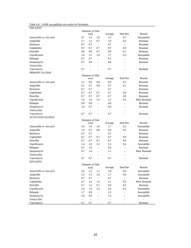
41

Table A.6. LWRP susceptibility test results for November. INFLUENT

Diameter of Disk

(cm) Average Stnd Dev Results Amoxicillin w/ clav.acid 0.7 1.9 2.0 1.5 0.7 Susceptible Ampicillin 1.1 1.2 0.7 1.0 0.3 Resistant Bacitracin 0.7 0.7 - 0.7 - Resistant Cephalothin 0.7 0.7 0.7 0.7 0.0 Resistant Penicillin 0.8 0.8 0.7 0.8 0.1 Resistant Ciprofloxacin 2.0 1.5 1.6 1.7 0.3 Susceptible Rifampin 0.7 0.7 - 0.7 - Resistant Streptomycin 0.7 0.8 - 0.8 - Resistant Tetracycline - - - - - - Vancomycin 0.7 - - 0.7 - Resistant PRIMARY SLUDGE

Diameter of Disk

(cm) Average Stnd Dev Results Amoxicillin w/ clav.acid 1.1 0.8 0.8 0.9 0.2 Resistant Ampicillin 0.7 0.7 0.8 0.7 0.1 Resistant Bacitracin 0.7 0.7 - 0.7 - Resistant Cephalothin 0.7 0.7 0.7 0.7 0.0 Resistant Penicillin 0.7 0.7 0.7 0.7 0.0 Resistant Ciprofloxacin 1.0 1.0 1.5 1.2 0.3 Mod. Resistant Rifampin 0.8 0.8 - 0.8 - Resistant Streptomycin 1.0 0.7 - 0.9 - Resistant Tetracycline - - - - - - Vancomycin 0.7 0.7 - 0.7 - Resistant ACTIVATED SLUDGE

Diameter of Disk

(cm) Average Stnd Dev Results Amoxicillin w/ clav.acid 1.6 1.6 2.0 1.7 0.2 Susceptible Ampicillin 1.2 0.7 0.8 0.9 0.3 Resistant Bacitracin 0.7 0.7 - 0.7 - Resistant Cephalothin 0.7 0.7 0.7 0.7 0.0 Resistant Penicillin 0.7 0.7 0.7 0.7 0.0 Resistant Ciprofloxacin 1.4 2.0 1.2 1.5 0.4 Susceptible Rifampin 0.7 1.0 - 0.9 - Resistant Streptomycin 0.7 1.4 - 1.1 - Mod. Resistant Tetracycline - - - - - - Vancomycin 0.7 0.7 - 0.7 - Resistant EFFLUENT

Diameter of Disk

(cm) Average Stnd Dev Results Amoxicillin w/ clav.acid 2.0 2.2 1.1 1.8 0.6 Susceptible Ampicillin 1.5 1.3 2.4 1.7 0.6 Susceptible Bacitracin 0.7 0.7 - 0.7 - Resistant Cephalothin 0.7 1.0 1.6 1.1 0.5 Mod. Resistant Penicillin 0.7 1.2 0.7 0.9 0.3 Resistant Ciprofloxacin 2.4 1.4 2.2 2.0 0.5 Susceptible Rifampin 1.7 0.9 - 1.3 - Susceptible Streptomycin 1.6 0.9 - 1.3 - Susceptible Tetracycline - - - - - - Vancomycin 0.7 0.7 - 0.7 - Resistant

42

Table A.7. LWRP susceptibility test results for December. INFLUENT Diameter of Disk (cm) Average Stnd Dev Results Amoxicillin w/ clav.acid 0.9 0.9 0.9 0.9 0.0 Resistant Ampicillin 0.7 0.7 0.8 0.7 0.1 Resistant Bacitracin 0.7 0.7 0.7 0.7 0.0 Resistant Cephalothin 0.8 0.7 0.7 0.7 0.1 Resistant Penicillin 0.7 0.7 0.7 0.7 0.0 Resistant Ciprofloxacin 1.2 1.1 1.0 1.1 0.1 Mod. Resistant Rifampin 0.7 0.7 0.8 0.7 0.1 Resistant Streptomycin 0.7 0.7 0.8 0.7 0.1 Resistant Tetracycline - - - - - - Vancomycin 0.7 0.7 0.7 0.7 0.0 Resistant PRIMARY SLUDGE Diameter of Disk (cm) Average Stnd Dev Results Amoxicillin w/ clav.acid 0.9 1.0 1.0 1.0 0.1 Resistant Ampicillin 0.7 0.8 0.8 0.8 0.1 Resistant Bacitracin 0.7 0.7 - 0.7 - Resistant Cephalothin 0.7 0.7 0.7 0.7 0.0 Resistant Penicillin 0.7 0.7 0.7 0.7 0.0 Resistant Ciprofloxacin 1.5 1.5 1.1 1.4 0.2 Susceptible Rifampin 1.1 1.1 - 1.1 - Mod. Resistant Streptomycin 0.8 0.8 - 0.8 - Resistant Tetracycline - - - - - - Vancomycin 0.7 0.7 - 0.7 - Resistant ACTIVATED SLUDGE Diameter of Disk (cm) Average Stnd Dev Results Amoxicillin w/ clav.acid 1.0 1.6 1.4 1.3 0.3 Susceptible Ampicillin 0.8 0.7 0.7 0.7 0.1 Resistant Bacitracin 0.8 0.8 - 0.8 - Resistant Cephalothin 0.7 0.7 0.7 0.7 0.0 Resistant Penicillin 0.7 0.7 0.8 0.7 0.1 Resistant Ciprofloxacin 1.2 1.2 1.2 1.2 0.0 Mod. Resistant Rifampin 0.9 0.8 - 0.9 - Resistant Streptomycin 1.6 1.1 - 1.4 - Susceptible Tetracycline - - - - - - Vancomycin 0.7 0.7 - 0.7 - Resistant EFFLUENT Diameter of Disk (cm) Average Stnd Dev Results Amoxicillin w/ clav.acid 2.8 2.0 1.0 1.9 0.9 Susceptible Ampicillin 1.0 1.4 2.0 1.5 0.5 Susceptible Bacitracin 0.7 1.0 1.6 1.1 0.5 Resistant Cephalothin 1.4 0.9 0.7 1.0 0.4 Resistant Penicillin 2.0 1.0 0.7 1.2 0.7 Resistant Ciprofloxacin 2.0 1.6 2.2 1.9 0.3 Susceptible Rifampin 1.5 1.2 0.7 1.1 - Mod. Resistant Streptomycin 3.1 1.8 2.0 2.3 - Susceptible Tetracycline - - - - - - Vancomycin 0.7 1.0 0.9 0.9 - Resistant

Urban Forested Wetland Restoration

Basic Information

Title: Urban Forested Wetland Restoration



End Date: 2/1/2003


Congressional District: 3rd


Focus Category: Wetlands, Ecology, Hydrology

Descriptors: None

Principal Investigators: Matthew Simmons, Steve Whisenant

Publication

1. Simmons, Matthew. Urbanizing Watersheds and Changing River Flood Dynamics: Implications forUrban Wetland Restoration. Texas Water Resources Institute SR 2003-016.

2. Simmons, Matthew, X. Ben Wu, and Steve Whisenant. Structure and Function of Old-growth andDisturbed Bottomlands Near Dallas, TX. Texas Water Resources Institute SR 2003-002.

Simmons 1

URBANIZING WATERSHEDS AND CHANGING RIVER FLOOD DYNAMICS:

IMPLICATIONS FOR URBAN WETLAND RESTORATION

MATTHEW SIMMONS1

Department of Rangeland Ecology and Management, Texas A&M University, College Station,

Texas 77843 USA

Abstract. Urbanization alters rive r hydrology, morphology, water quality, and habitat and

ecology. Most of these associated changes are due to an increase in impervious surface cover

(ISC) throughout the watershed. But the spatial location of urban areas within the watershed also

greatly influences river hydrology. As river hydrology changes, functions and structure of

riverine wetlands associated with the hydrology may be impacted. In order to increase the long-

term success of wetland restoration attempts within an urbanizing environment, it is necessary to

quantify potential impacts to the wetlands as hydrology continues to change. This study

investigated the effects of increased ISC on stream hydrology between 1972 and 1995 for a sub-

watershed located north of Dallas, Texas. Moving window and FRAGSTATS analyses

calculated the degree and location of ISC throughout the basin, and U.S. Geologic Survey

stream-gauge data were analyzed to determine changes in steam hydrology between the 2 time

periods. Average ISC for the watershed increased from 2 to 11% between 1972 and 1995, but

highest cover (50–80%) occurred along the southern and eastern borders. Annual river flooding

frequency and duration doubled between 1972 and 1995, and flooding velocity increased from

31.4 to 35.4 m3/sec. Wetland restoration attempts within the watershed should address the

potential for future hydrologic changes as ISC continues to increase.

Key words: urbanization; impervious surface cover; wetlands; wetland restoration; hydrologic

regime

INTRODUCTION

The process of urbanization impacts streams in many ways that include alterations to

hydrology, morphology, water quality, and habitat and ecology (Schueler 1992). Changes to

these stream attributes are caused by an increase of impervious surface cover (ISC) associated

1 [email protected]

Simmons 2

with the process of urbanization. With increasing ISC, soil water infiltration decreases, which

increases surface runoff. The degree of urban surface runoff is typically proportional to the

amount of ISC. For example, as ISC reaches 10–20% within a catchment basin, runoff increases

twofold; 35–50% ISC causes a threefold increase in runoff; and 75–100% ISC increases surface

runoff more than fivefold over forested regions (Arnold and Gibbons 1996).

The increased runoff associated with urbanization affects stream hydrology in many

ways. The time lag between the center of the precipitation event to the center of the peak flow

discharge decreases as urbanization increases (Espey et al. 1965). Stream velocity and the

associated erosive forces increase, as do the magnitude and frequency of flooding events

(Schueler 1992).

Although the degree of urbanization, as measured by the percent cover of impervious

surface cover, is one of the most important factors determining stream hydrography, the location

of urbanization within the watershed also plays an important role. Sheeder et al. (2002) found

dual urban and rural hydrograph peaks based on the degree and spatial location of urbanization

within the watershed. The first peak is a result of drainage from the urban area followed closely

by drainage from the rural area. Although not addressed in the article, flood duration may

increase as a result of the two flooding peaks occurring consecutively. Hirsch et al. (1990)

theorize that if lower reaches of a basin become urbanized with little development in the upper

basin, water from the lower urban portion could drain before the arrival of water from the upper

portion, thus decreasing flooding magnitude but increasing duration.

The effects of urbanization on stream hydrology can have serious implications for the

long-term sustainability and health of riverine wetlands. Riverine wetlands are those located

within floodplains of rivers and streams. As hydrology is the most important determinant of

wetland structure and function (Mitsch and Gosselink 2000), and because the hydroperiod of

riverine wetlands are inextricably connected with the flooding regime of the associated river, an

altered hydroperiod caused by urbanization may significantly alter wetland structure and

function that had developed under pre-urban conditions.

Not only is the changing hydrology an important consideration for potential impacts on

urban wetlands, but this has important implications for urban wetland restoration attempts as

well. Most wetland restoration failures have been attributed to a failure to restore a proper

hydrologic regime (Kunz et al. 1988, Kusler 1990, Mitsch and Gosselink 2000, Stolt et al. 2000).

Simmons 3

For example, restoration projects resulting in wetlands becoming too wet for bottomland species

may limit above ground production, while those resulting in dry conditions may not support

obligate wetland species (Niswander and Mitsch 1995). Wetland restoration attempts within

urbanizing watersheds need to consider the changing hydrology in order to ensure hydrologic

levels suitable for optimal wetland production. Hydrologic conditions at the time of restoration

may be very different from those some years down the road as urbanization within the watershed

continues to increase. It is, therefore, imperative to quantify the degree and location of

urbanization within the watershed with the associated hydrologic alterations over time, and be

able to predict future hydrologic impacts based on past and present land-use changes.

A bottomland hardwood forest restoration project is currently being undertaken in Dallas

County, Texas. As urbanization within the watershed has increased, river hydrologic regimes

have been altered. Because the potential for continued urbanization exis ts, it is necessary to

quantify past land use change to predict impacts of future land use changes on the restored

wetland. The objectives of this study were to (1) determine the location and degree of

urbanization within the East Fork Trinity watershed before and during urbanization and relate it

to hydrologic changes of Rowlett Creek, which is located within the watershed, and (2) given the

degree of urbanization and hydrologic alteration, determine necessary steps to take to ensure the

long-term success of restored wetlands within the watershed.

METHODS

Study area

The East Fork Trinity watershed is located north of Dallas, Texas, in Dallas and Collin

counties and was delineated by the US Environmental Protection Agency (2002). A sub-

watershed within the East Fork Trinity watershed was derived from a digital elevation model

with 30-m resolution to limit the watershed to include only the hydrologic area of interest

directly influenced by urbanization. The extent of this watershed is 374 km2.

The climate of the region includes mild winters and hot summers averaging 9º and 29ºC,

respectively. Average annual precipitation is 94 cm, which occurs throughout the year but peaks

slightly during the spring (NOAA 2003). The Dallas metropolitan area has experienced rapid

urban growth, as much as 400% since 1970 (Knauss 2001).

Simmons 4

Image preparation and analysis

Aerial photographs from 1972 were used for pre-urban analyses. DOQQs from 1995

with 1-m resolution were downloaded from the Texas Natural Resources Information System

website (TNRIS 2003) for use of comparison to the 1972 photos. It became apparent that time

would limit the amount of the watershed that could be analyzed for this study. Consequently, a

sub-watershed was then chosen based on its small size (31 km2) and close proximity to the U.S.

Geologic Survey (USGS) stream-gauge station used for the hydrologic analyses.

Land cover types for the grids created from the photos and DOQQs were classified using

unsupervised classification in ERDAS IMAGINE 8.6 (ERDAS IMAGINE 2002). The resulting

50 classes were then manually combined into 5 classes based on visual estimates from the photos

and DOQQs. These cover classes included woody, herbaceous, bare ground, impervious surface,

and water. The classification was still not entirely accurate as much of the actual water and

herbaceous cover were classified as woody. These areas were subsequently manually delineated

and appropriately reclassified.

The amount of cover of each class was determined for the entire sub-watershed in

ArcView (ESRI 1998), but because spatial location of urbanization within a watershed is also

important in determining hydrologic changes over time, a moving window approach was used in

combination with FRAGSTATS v. 3 (McGarigal and Marks 1995) to determine patch attributes

at a finer scale. Patch attributes calculated included cover, number of patches, mean patch size,

and edge density.

Moving windows with a 356-m radius were systematically shifted in 178-m steps across

the classified grids. At least 50% of each window needed to include data from within the sub-

watershed in order to be included in the analyses. An ArcView script was then used to perform

the FRAGSTATS metrics in all moving windows.

Hydrologic analyses

To compare hydrologic changes over time, stream-gauge data for Rowlett Creek were

downloaded from the USGS website (NWISWeb Data for USA 2003). Analysis of the data

included 5-year intervals centered on the 2 dates for which aerial photos and DOQQs were

available, 1972 and 1995, respectively. Annual flooding frequency and duration were calculated

for 2 flooding heights, 28 and 89 cm above base flow elevations. The average duration of a

Simmons 5

single flooding event was calculated by dividing the total annual flood duration by the number of

annual floods. Average flooding magnitude (m3/sec) of floods greater than 28 cm was also

calculated for each of the time periods.

RESULTS

Image analyses

Percent cover values of each cover class were calculated for the entire sub-watershed for

1972 and 1995 (Table 1). Percent woody cover almost doubled between years from 9 to 17%.

Because it was difficult to distinguish between bare ground and ISC during the classification

procedure, these 2 cover classes are listed both separately and combined. ISC alone increased

over fivefold between years from 2 to 11%, while combining bare ground and ISC resulted in a

little under double the cover in 1995 compared to 1972 (8 to 15%).

Table 1. Percent cover of different land-cover classes summarized for the entire sub-

watershed in 1972 and 1995.

1972 1995

Woody 9% 17%

Herbaceous 81% 67%

Bare ground + ISC 8% 15%

Bare ground 6% 4%

ISC 2% 11%

Water 0.8% 1.2%

Results of FRAGSTATS analyses showed differing changes in cover for different areas

of the sub-watershed between years. Percent woody cover as well as the size and numbers of

woody patches have increased over much of the sub-watershed (Fig. 1). Edge density also

increased between years (Fig. 1d). The most pronounced increases in numbers and cover of

woody patches in 1995 were centered around areas where patch number and cover were highest

in 1972.

An increase in ISC between years was mainly restricted to a few scattered areas

throughout the sub-watershed (Fig. 2). ISC cover was highest in 1995 along the southern and

Simmons 6

eastern edges of the basin (Fig. 2a). These areas are located close to the mouth of the basin. The

number of ISC patches increased between years, but the mean patch size decreased (fig. 2b, c).

These results, in combination with high edge densities of 3000/ha (Fig. 2d), indicate that ISC

increased but became more fragmented between years.

Hydrologic analyses

Because urbanization has a greater effect on smaller floods (Hirsch et al. 1990), analyses

of flooding frequency and duration were separated into small floods (28 cm) and larger floods

(89 cm). Despite this separation, both annual flooding frequency and duration of Rowlett Creek

doubled between years for both heights (Table 2).

Table 2. Average annual flooding frequency and duration for small and larger floods

for 2 time periods. The data represent 5-yr averages centered on 1972 and 1995.

Frequency (#/yr) Duration (days/yr)

1972 1995 1972 1995

Small floods (28 cm) 9.6 18.4 15.8 31.6

Larger floods (89 cm) 4.6 8.8 6 11.4

Disregarding flooding height, the average duration for a single flooding event increased

from 40 hrs to 42hrs between 1972 and 1995. The average flood velocity remained the same

between the 2 time periods (Fig. 3), but when extreme low and high floods were discounted

flood velocities increased from 31.4 to 35.4 m3/sec.

Simmons 7

Figure 1. Results of FRAGSTATS analyses for woody cover within the sub-watershed

performed on grids generated from moving window analyses. Figures in the left column refer to

1972 and those in the right to 1995. (a) Percent cover, (b) number of patches, (c) mean patch

size, and (d) edge density.

b. No. of patches

1995 1972 a. Percent Cover

c. Mean Patch Size (ha)

d. Edge Density (#/ha)

0 2km

4

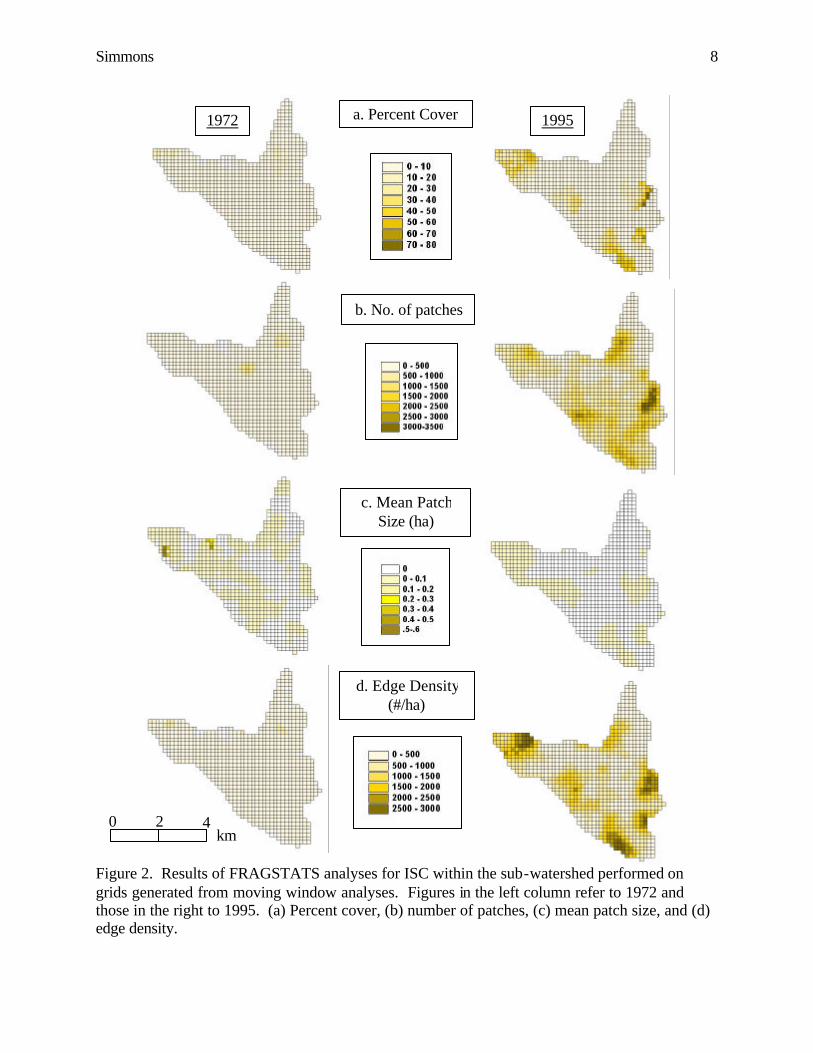
Simmons 8

Figure 2. Results of FRAGSTATS analyses for ISC within the sub-watershed performed on grids generated from moving window analyses. Figures in the left column refer to 1972 and those in the right to 1995. (a) Percent cover, (b) number of patches, (c) mean patch size, and (d) edge density.

1995 1972 a. Percent Cover

0 2km

4

b. No. of patches

c. Mean Patch Size (ha)

d. Edge Density (#/ha)

Simmons 9

Flooding Magnitude for the 1970s and 1990s

29

30

31

32

33

34

35

36

Average Median & Mode

1970s

1990s

Figure 3. Average, median, and mode flooding magnitude for

the 5-yr periods from 1970 to 1974 and 1993 to 1997.

DISCUSSION

The results of the FRAGSTATS analyses seem initially counterintuitive. Woody cover

increased with an increase in number of patches and patch size, while ISC increased with

increasing number of patches but decreasing patch size. One would expect that as urbanization

increases, ISC patch size would also increase and woody cover would decrease. These results

can be explained by 2 phenomena: (1) land that was used for agriculture had been cleared of

woody cover, but the conversion to urban land allowed woody cover to increase, and (2) this

doubling of woody cover would appear to fragment the ISC from an aerial photo or DOQ, thus

creating smaller ISC patch sizes. Viewing the original 1972 aerial photos revealed very little

woody cover in presumably newly developed urban areas. By 1995, the trees had grown to an

extent that they covered housetops and streets, thereby fragmenting ISC. Analyses of patch

attributes may have yielded more accurate results had the woody patches within ISC patches

been discounted.

Spatial location of urban patches varied throughout the sub-watershed. This spatial

complexity makes it difficult to directly relate the influence of spatial location of ISC to specific

hydrologic variables. However, a clear relationship does exist between changes in the amount of

ISC and changes to the hydrologic regime. In 1972, only 2% of the sub-watershed was covered

by ISC. In 1995, ISC increased to 11%. By that time annual flooding frequency and duration

had doubled, and average flooding magnitude and single flood duration also increased.

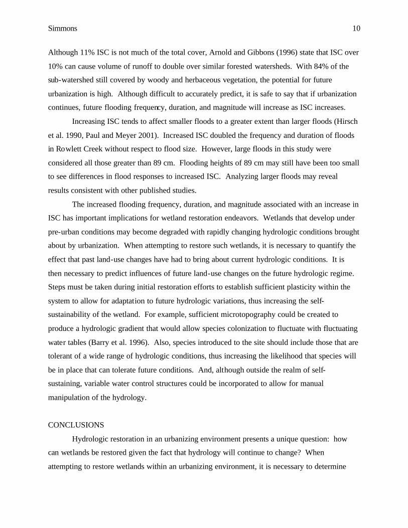
Simmons 10

Although 11% ISC is not much of the total cover, Arnold and Gibbons (1996) state that ISC over

10% can cause volume of runoff to double over similar forested watersheds. With 84% of the

sub-watershed still covered by woody and herbaceous vegetation, the potential for future

urbanization is high. Although difficult to accurately predict, it is safe to say that if urbanization

continues, future flooding frequency, duration, and magnitude will increase as ISC increases.

Increasing ISC tends to affect smaller floods to a greater extent than larger floods (Hirsch

et al. 1990, Paul and Meyer 2001). Increased ISC doubled the frequency and duration of floods

in Rowlett Creek without respect to flood size. However, large floods in this study were

considered all those greater than 89 cm. Flooding heights of 89 cm may still have been too small

to see differences in flood responses to increased ISC. Analyzing larger floods may reveal

results consistent with other published studies.

The increased flooding frequency, duration, and magnitude associated with an increase in

ISC has important implications for wetland restoration endeavors. Wetlands that develop under

pre-urban conditions may become degraded with rapidly changing hydrologic conditions brought

about by urbanization. When attempting to restore such wetlands, it is necessary to quantify the

effect that past land-use changes have had to bring about current hydrologic conditions. It is

then necessary to predict influences of future land-use changes on the future hydrologic regime.

Steps must be taken during initial restoration efforts to establish sufficient plasticity within the

system to allow for adaptation to future hydrologic variations, thus increasing the self-

sustainability of the wetland. For example, sufficient microtopography could be created to

produce a hydrologic gradient that would allow species colonization to fluctuate with fluctuating

water tables (Barry et al. 1996). Also, species introduced to the site should include those that are

tolerant of a wide range of hydrologic conditions, thus increasing the likelihood that species will

be in place that can tolerate future conditions. And, although outside the realm of self-

sustaining, variable water control structures could be incorporated to allow for manual

manipulation of the hydrology.

CONCLUSIONS

Hydrologic restoration in an urbanizing environment presents a unique question: how

can wetlands be restored given the fact that hydrology will continue to change? When

attempting to restore wetlands within an urbanizing environment, it is necessary to determine

Simmons 11

changes in the degree and spatial location of urbanization over time. This study has shown that

flooding frequency, duration, and magnitude increased as urbanization increased. It is important

to note that these conclusions were based on analyses completed on a portion of the watershed.

However, it is safe to say that as urbanization continues flooding dynamics will continue to

change. Instead of fighting against them, allowing the system to respond to these changes, by

creating hydrologic gradients, introducing species with wide environmental tolerances, and

installing variable water control structures, will increase the probability of continued restoration

success.

ACKNOWLEDGEMENTS

Special thanks are extended to Paikho Rho and Humberto Perotto for their assistance

with software applications and advice on proper remote-sensing methodologies. Funding for this

project was supported by the Department of Rangeland Ecology and Management, the City of

Garland, Texas, and the Texas Water Resources Institute.

LITERATURE CITED

Arnold, C. L., and C. J. Gibbons. 1996. Impervious surface coverage: the emergence of a key

environmental indicator. Journal of the American Planning Association 62:243–258.

Barry, W. J., A. S. Garlo, and C. A. Wood. 1996. Duplicating the mound-and-pool

microtopography of forested wetlands. Restoration & Management Notes 14:15–21.

ERDAS IMAGINE. 2002. ERDAS Field Guide Sixth Edition. Leica Geosystems, Atlanta,

Georgia, USA.

Espey, W. H., C. W. Morgan, and F. D. Masch. 1965. A study of some effects of urbanization

on storm runoff from a small watershed. Center for Research in Water Resources,

University of Texas, Austin, Texas, USA.

ESRI (Environmental System Research Institute). 1998. ArcView GIS 3.2a. Environmental

Systems Research Institute, Inc., Redlands, California, USA.

Hirsch, R. M., J. F. Walker, J. C. Day, and R. Kallio. 1990. The influence of man on hydrologic

systems. Pages 329–359 in M. G. Wolman and H. C. Riggs, editors. Surface water

hydrology (The Geology of North America, Volume 0-1). The Geologic Society of

America, Boulder, Colorado, USA.

Simmons 12

Knauss, Philip. 2001. Growth trends in the Dallas-Fort Worth metropolitan statistical area.

http://www.ace.uiuc.edu/Classes/up406/samples/1KnausDAL2001.PDF, University of

Illinois, Champaign-Urbana, Illinois, USA.

Kunz, K., M. Rylko, and E. Somers. 1988. An assessment of wetland mitigation practices

in Washington State. National Wetlands Newsletter 10:2–4.

Kusler, J. A. 1990. Views on scientific issues relating to restoration and creation of

wetlands. Pages 217–230 in G. Bingham, E. H. Clark, L. V. Haywood, and M. Leslie,

editors. Issues in wetland protection. The Conservation Foundation, Washington D.C.,

USA.

McGarigal, K., and B. J. Marks. 1995. FRAGSTATS: Spatial pattern analysis program for

quantifying landscape structure. USDA Forest Service, General Technical Report PNW-

351.

Mitsch, W. J., and J. G. Gosselink. 2000. Wetlands. Third edition. John Wiley & Sons,

New York, New York, USA.

Niswander, S. F., and W. J. Mitsch. 1995. Functional analysis of a two-year-old created

in-stream wetland: hydrology, phosphorous retention, and vegetation survival and

growth. Wetlands 15:212–225.

NOAA (National Oceanic and Atmospheric Administration). 2003. Climate,

http://www.noaa.gov/climate.html.

NWISWeb Data for USA. 2003. http://waterdata.usgs.gov/nwis.

Paul, M. J., and J. L. Meyer. 2001. Stream in the urban landscape. Annual Review of

Ecology and Systematics 32:333–365.

Sheeder, S. A., J. D. Ross, and T. N. Carlson. 2002. Dual urban and rural hydrograph signals in

three small watersheds. Journal of the American Water Resources Association 38:1027–

1040.

Schueler, T. R. 1992. Mitigating the adverse impacts of urbanization on streams: a

comprehensive strategy for local governments. Pages 21–31 in P. Kumble and T.

Schueler, editors. Watershed restoration sourcebook. Metropolitan Council of

Governments, College Park, Maryland, USA.

Stolt, M. H., M. H. Genthner, W. L. Daniels, V. A. Groover, S. Nagle, and K. C. Hearing.

Simmons 13

2000. Comparison of soil and other environmental conditions in constructed and

adjacent palustrine reference wetlands. Wetlands 20:671–683.

TNRIS. 2003. Texas Natural Resources Information System, http://www.tnris.state.tx.us/.

US Environmental Protection Agency. 2002. Surf your watershed, http://www.epa.gov/surf/.

Adsorption and Desorption of Atrazine on Selected LakeSediments in Texas

Basic Information

Title: Adsorption and Desorption of Atrazine on Selected Lake Sediments in Texas



End Date: 2/1/2003




Focus Category: Agriculture, Surface Water, Sediments

Descriptors: None

Principal Investigators: Judy A. Vader, Scott Senseman

Publication

1. Vader, J. A., S. A. Senseman, and M. C. Dozier. Adsorption and Desorption of Atrazine fromVarious Lake Sediments in Texas. Texas Water Resources Institute SR 2003-004.

Adsorption and Desorption of Atrazine from Various Lake

Sediments in Texas

Report

Judy A. Vader

June 1, 2003

Department of Soil and Crop Science

Texas A&M University

College Station, Texas

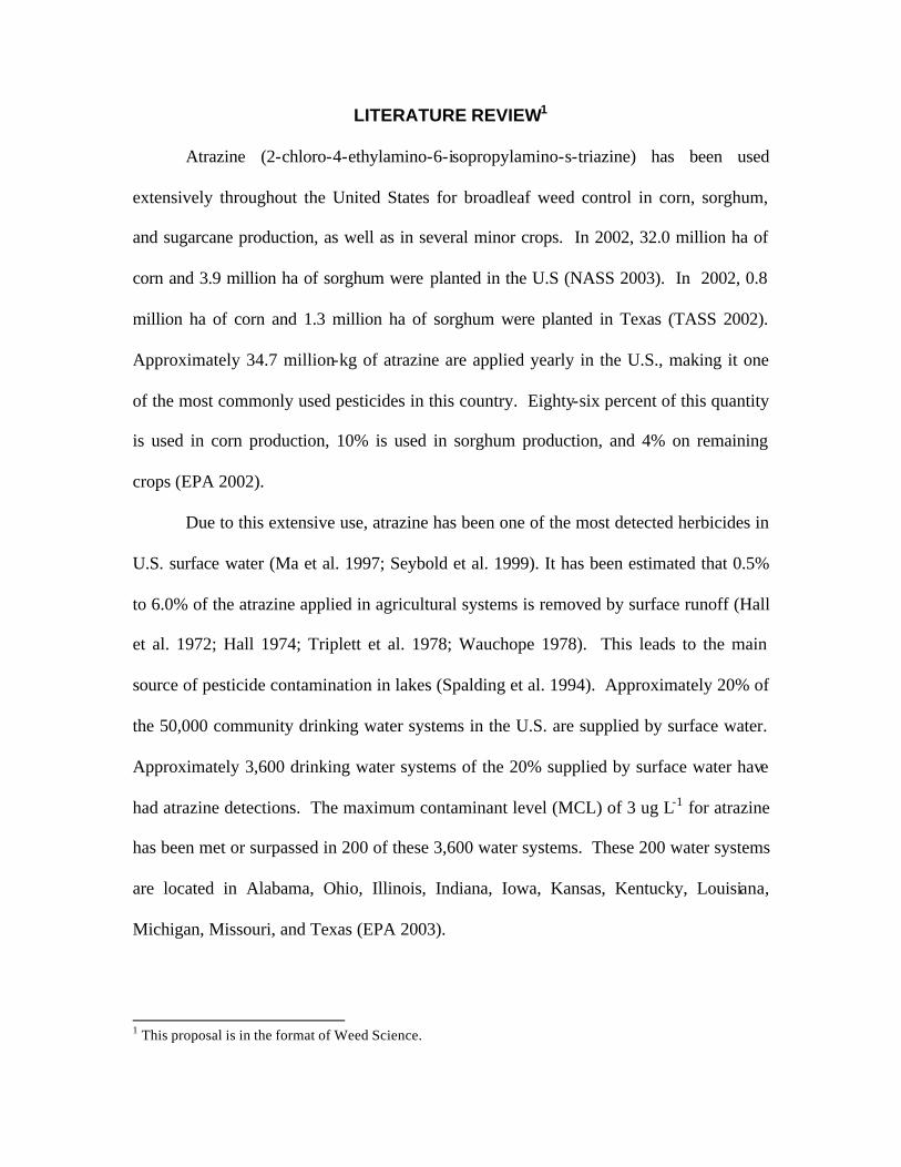
LITERATURE REVIEW1

Atrazine (2-chloro-4-ethylamino-6-isopropylamino-s-triazine) has been used

extensively throughout the United States for broadleaf weed control in corn, sorghum,

and sugarcane production, as well as in several minor crops. In 2002, 32.0 million ha of

corn and 3.9 million ha of sorghum were planted in the U.S (NASS 2003). In 2002, 0.8

million ha of corn and 1.3 million ha of sorghum were planted in Texas (TASS 2002).

Approximately 34.7 million-kg of atrazine are applied yearly in the U.S., making it one

of the most commonly used pesticides in this country. Eighty-six percent of this quantity

is used in corn production, 10% is used in sorghum production, and 4% on remaining

crops (EPA 2002).

Due to this extensive use, atrazine has been one of the most detected herbicides in

U.S. surface water (Ma et al. 1997; Seybold et al. 1999). It has been estimated that 0.5%

to 6.0% of the atrazine applied in agricultural systems is removed by surface runoff (Hall

et al. 1972; Hall 1974; Triplett et al. 1978; Wauchope 1978). This leads to the main

source of pesticide contamination in lakes (Spalding et al. 1994). Approximately 20% of

the 50,000 community drinking water systems in the U.S. are supplied by surface water.

Approximately 3,600 drinking water systems of the 20% supplied by surface water have

had atrazine detections. The maximum contaminant level (MCL) of 3 ug L-1 for atrazine

has been met or surpassed in 200 of these 3,600 water systems. These 200 water systems

are located in Alabama, Ohio, Illinois, Indiana, Iowa, Kansas, Kentucky, Louisiana,

Michigan, Missouri, and Texas (EPA 2003).

1 This proposal is in the format of Weed Science.

Due to the detections in Texas, some monitoring programs have been initiated.

Eight lakes around the Dallas area of North Texas, were analyzed by the Texas A&M

Pesticide Fate Laboratory in College Station, TX for the presence of atrazine in the lake

water. These eight lakes consisted of Big Creek Lake, Joe Pool Lake, Lavon Lake,

Bardwell Lake, Lake Waxahachie, Lake Aquilla, Lake Tawakoni, and Richland-

Chambers Reservoir. Concentrations have primarily ranged from 0.3 ug L-1 to 0.5 ug L-1

through out the year in the source water of these lakes. Occasionally, concentrations

have ranged from 30 to 50 ug L-1 atrazine during the spring months following atrazine

applications. Higher concentrations of pesticides typically have been found in both

ground and surface water following initial herbicide application (Pionke et al.1990;

Spalding et al. 1989; Triplett et al.1978; Wauchope 1978; Wu et al. 1983). All eight

lakes have been placed on the Texas 2000 Clean Water Act Section 303(d) list because

the atrazine concentrations in finished drinking water indicated contamination of source

water. Seven of these lakes were classified as “threatened” lakes meaning that the

finished drinking water from these lakes had a concentration of 1.5 ug L-1 atrazine or

50% of the MCL. Aquilla Lake was classified as an impaired body of water due to the

fact that its finished drinking water exceeded the MCL of 3 ug L-1 (TNRCC 2002).

Although not deemed a human carcinogen, atrazine has become a growing

concern regarding human and wildlife health due to its presence in surface water. Sexual

abnormalities in frogs and a decrease in length and weight have been linked to atrazine

contamination (Carr et al. 2003; Diana et al. 2000; Morgan 1996; Reeder et al. 1998;

Tavera-Mendoza 2002). Lab studies on frogs have shown observed sexual abnormalities

at atrazine concentrations of >20 ug L-1. Above 200 ug L-1 of atrazine, both frog length

and weight decreased (Diana et al. 2000). High atrazine concentrations had no effect on

survival (Diana et al. 2000). It was concluded in these studies that atrazine

concentrations in natural water were too low to cause a threat to wildlife (Carr et al.

2003; Diana et al. 2000; Morgan 1996; Reeder et al. 1998; Tavera-Mendoza 2002).

Recently it was reported that concentrations as low as 0.1 ug L-1 were shown to cause

sexual abnormalities in frogs in the laboratory (Hayes et al. 2002). This concentration is

below the EPA’s MCL. The same study reported seeing frog abnormalities in natural

water at concentrations ranging from 0.2 ug L-1 and greater although no other

contaminants were studied (Hayes et al. 2002). A study on cricket frogs (Acris crepitans)

concluded that 2.7% of frogs collected from different sites in Illinois during a 3-year

period were intersexed. Along with atrazine, polychlorinated biphenyl (PCB) and

polychlorinated dibenzofuron (PCDF) were found in the samples collected (Reeder et al.

1998). More research is needed to determine if atrazine is the sole cause of such

abnormalities.

Atrazine, a symmetrical triazine, has several different fates in lake water

including hydrolysis, photolysis, adsorption, and desorption (Gao et al. 1998; Goswami

et al. 1971; Konstantinou et al. 2001; Mersie et al. 1998a; Moreau et al. 1997; Wauchope

et al. 1985). Atrazine has a relatively low water solubility (33 mg L-1) and moderate

adsorption (average Koc = 100 ml g-1), but little is known about the interaction of atrazine

and sediment (Mersie et al. 1998b). Along with atrazine, three of its metabolites have

been found in lake water (EPA 2003). These metabolites are desethyl atrazine (DEA),

desisopropyl atrazine (DIA), and diaminochlorotriazine (DACT).

Often sediment has been questioned as a potential storage reservoir, transport

vehicle, and ultimately a long-term contamination source of organic compounds like

atrazine. Adsorption and desorption of organic compounds to soil depends on several

different factors, including sand, silt, and clay contents, organic matter, pH, and aerobic

and anaerobic environment. Soil and water pH plays a primary role in the adsorption

behavior of atrazine. As pH decreases, the cationic fraction is increased, increasing

atrazine adsorption to soil (Clay et al. 1990a; Gao et al. 1998; Rae et al. 1998; Weber

1970). Likewise, atrazine tends to desorb as pH increases (Jenks et al. 1998).

Atrazine adsorbs to both organic matter and clays. Organic matter has a greater

affinity to atrazine compared to clay (Gao et al.1998; Laird et al. 1994; Ying et al. 2000).

Atrazine affinity to soil increases as organic matter increases (Patakioutas et al. 2002).

This increase in organic matter decreases the amount desorbed (Jenks et al. 1998).

A decrease in soil particle size increases the adsorption of atrazine to soil and

decreases the amount susceptible to desorption. Its high affinity to clay and silt particles

is greater due to greater surface area compared with coarser textures (Sonon et al. 1995).

However, if pH decreases and organic matter increases, or a combination of the two, the

affinity of a sandy soil to atrazine increases (Gao et al. 1998).

In several studies, it has been shown that the total amount of atrazine adsorbed to

a soil or sediment is not completely desorbed. Normally small fractions (5.5 to 40 %) of

the amount adsorbed were desorbed demonstrating that relatively large amounts of

atrazine potentially are adsorbed or degraded (Clay 1990b; Gao 1998; Jenks et al. 1998;

Pignatello et al. 1991; Seybold 1996).

As in soils, sediments may have different adsorptive characteristics and, therefore,

may have different affinities for organic compounds like atrazine. Unlike soil, sediment

is found in an anaerobic environment and often contains a greater amount of organic

matter, which may affect adsorption capacities of sediments (Seybold 1999).

A classification system for adsorption isotherms was designed by Giles et al.

(1960). This design classified adsorption patterns of soils in four different categories.

The different isotherms included the S, C, L, and H-type isotherms. The S-type occurs

where lower concentrations of the pesticide remain in water, mid- level concentrations

adsorb, and high concentrations reach a maximum adsorption. The C-type isotherm,

demonstrates constant partitioning of a compound across a range of concentrations and a

maximum adsorption is never reached. The L-type isotherm (Langmuir) demonstrates a

relatively high affinity at lower concentrations, but then reaches maximum adsorption at

higher concentrations. The H-type isotherm (high affinity) is similar to the L-type but

has a higher affinity at low concentrations and reaches a maximum (Weber 1970).

The difference between the amount of a herbicide adsorbed to a soil or sediment

and the amount of the herbicide desorbed from the same soil or sediment is known as

hysteresis. No one mechanism influences the adsorption and desorption process of a

compound in the same way. Several types of bonds, varying in strength between the

sediment and herbicide, can cause adsorption. The same bonds influences the herbicides

desorption. Bonds range from weak bonds such as London-van der Waals forces to

strong bonds such as covalent bonds. In desorption, the weaker bonds are broken, but the

stronger ones may not be over come. Without the release of these stronger bonds,

equilibrium during the desorption process is never met. This in part explains the amount

of certain herbicides, which remain adsorbed even after several desorption cycles

(Koskinen et al. 1990).

Another concern in the possible sediment storage and recontamination factor is

the degradation and persistence of atrazine once adsorbed to the sediment. Past studies,

have shown that the half- life of atrazine is variable among soils and sediments. The

average field half- life is 60 d, but the half- life has ranged from 39 d to 261 d (Vencill

2002). In sediments collected from estuarine water, atrazine’s half- life of 15 to 20 d was

reported (Jones et al. 1982), and a half- life of 145 d was reported from Wisconsin lake

sediments (Armstrong et al. 1967; Jones et al. 1982).

Many different factors contribute to atrazine degradation once adsorbed to soil.

Atrazine is susceptible to breakdown by UV light (photolysis) after application into

hydroxyatrazine and N-desethylated atrazine (Vencill 2002; Jordan et al. 1970).

Photolysis is faster in soil systems than in water because photolysis is hindered by the

presence of organic matter in surface water (Konstantinou et al. 2001). In soils at a

moderately acidic pH ranging between 5.5 to 6.5, atrazine degradation to hydroxyatrazine

is due to chemical hydrolysis, and at moderately neutral pH in soils, hydrolysis is

partially driven by an increase in microbial activity (Vencill 2002; Blumhorst et al.

1994). Hydrolysis is slower at more basic values ranging from 7.5 to 8 in soils (Vencill

2002; Blumhorst et al. 1994). In anaerobic environments, pH is typically higher than

aerobic situations and has a low rate of atrazine hydrolysis and also atrazine dealkylation

by microbes (Goswami et al. 1971; Jones et al. 1982; Klint et al. 1993).

Soil bacteria can drive microbial hydroxylation and mineralization. Some

Pseudomonas species have been observed to mineralize atrazine in both aerobic and

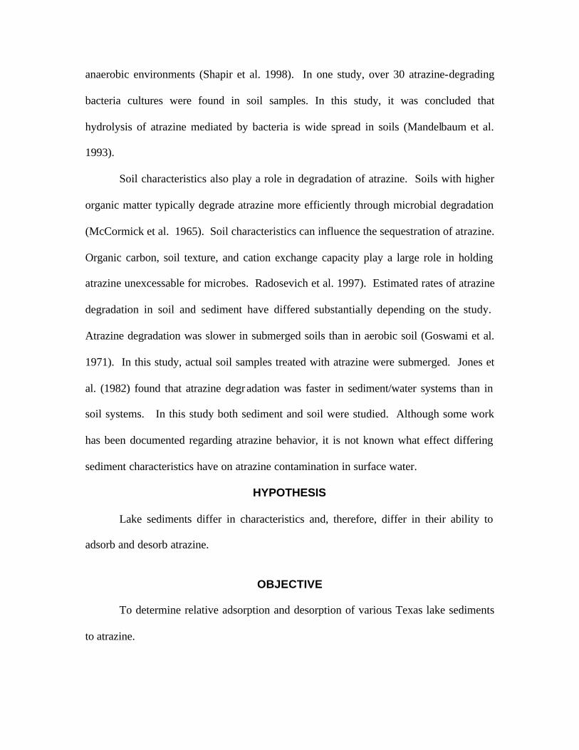
anaerobic environments (Shapir et al. 1998). In one study, over 30 atrazine-degrading

bacteria cultures were found in soil samples. In this study, it was concluded that

hydrolysis of atrazine mediated by bacteria is wide spread in soils (Mandelbaum et al.

1993).

Soil characteristics also play a role in degradation of atrazine. Soils with higher

organic matter typically degrade atrazine more efficiently through microbial degradation

(McCormick et al. 1965). Soil characteristics can influence the sequestration of atrazine.

Organic carbon, soil texture, and cation exchange capacity play a large role in holding

atrazine unexcessable for microbes. Radosevich et al. 1997). Estimated rates of atrazine

degradation in soil and sediment have differed substantially depending on the study.

Atrazine degradation was slower in submerged soils than in aerobic soil (Goswami et al.

1971). In this study, actual soil samples treated with atrazine were submerged. Jones et

al. (1982) found that atrazine degradation was faster in sediment/water systems than in

soil systems. In this study both sediment and soil were studied. Although some work

has been documented regarding atrazine behavior, it is not known what effect differing

sediment characteristics have on atrazine contamination in surface water.

HYPOTHESIS

Lake sediments differ in characteristics and, therefore, differ in their ability to

adsorb and desorb atrazine.

OBJECTIVE

To determine relative adsorption and desorption of various Texas lake sediments

to atrazine.

MATERIALS AND METHODS

Eight lake sediments were collected from sites where atrazine was detected during

an earlier study. All eight lakes were located in northeast Texas and were used as

community water use systems.

Sediment collection and preparation.

Sediment samples were collected using an Eckman dredge from a bridge or boat

depending on site availability at each individual lake. Samples were placed in 3.75-L

Ziploc bags and placed in a cooler for transport back to the laboratory. Once back at the

laboratory, samples were dried on paper in the greenhouse. The sediment samples were

then ground with a soil grinder and then a mortar and pestle as needed to get uniform

particle size. After grinding, sediments were passed through a 2-mm sieve. Subsamples

were characterized by the Texas A&M Soil Characterization Laboratory for texture,

percent organic carbon, pH, CEC, extractable bases, and % base saturation.

Batch equilibrium adsorption and desorption.

Four 2-g samples were weighed out for each collection and placed into separate

35-ml centrifuge tubes. Initial standard solutions were made using a ring- labeled atrazine

standard combined with an analytical grade atrazine standard in methanol. One hundred

uL of the initial standard solutions were added to each centrifuge tube along with 5-ml of

0.01M CaCl2 solution to provide a constant ionic strength during the adsorption-

desorption experiment. This provided a concentration of approximately 8.41 Bq mL-1 14C

material in all samples, and 0.5, 1.0, 2.0, and 5.0 ug mL-1 of analytical grade, non-radio

labeled atrazine.

The samples were placed on a table shaker and shaken for 24 h. Tubes were then

removed and centrifuged for 10 min. A 2-mL aliquot were then removed from the

supernant of each sample and placed in glass scintillation vials along with 10 ml of

scintillation fluid for the adsorption study. The remaining solution (1ml) was removed

from the samples and replaced with fresh 0.01M CaCl2 solution. Samples were then

shaken again for 24 h. Another 2-ml aliquot were removed and placed in glass

scintillation vials along with 10 ml of scintillation fluid for analysis of atrazine

desorption. The procedure was repeated two more times in a 48-h period. The aliquots

in scintillation fluid were then placed on a Beckman LS6500 Multipurpose scintillation

counter. Each sample was counted for 20 min.

The relative affinity of atrazine to a sediment was determined by the Freundlich

equation.

X/M = KC1/n (1)

log X/M = log K + 1/n log C (2)

Where, X/M equals the amount adsorbed per amount adsorbent, C represent the solution

concentration at equilibrium, and K and n are constants. K represents the affinity of the

herbicide to the sediment, and 1/n is the slope. If n is approximately 1, K represents the

distribution coefficient, Kd.

Isotherms were characterized, by graphing X/M on the y-axis and C on the x-axis.

Hysteresis was determined, by graphing the adsorption amounts using log X/M on the y-

axis and log C on the x-axis. Desorption of two initial concentrations of 1.0 ug mL-1 and

5.0 ug mL-1 were chosen to determine desorption behavior of atrazine from the selected

sediments. These desorption amounts were subtracted from the total amount adsorbed at

the specified concentration. The result was the amount of atrazine remaining adsorbed

after the consequent desorption steps. The difference between adsorption and desorption

showed the amount of atrazine that was desorbed. This also provided a way of

determining the degree of hysteresis.

The experiment was executed in a completely randomized block design and

replicated four times. Linear regression was used to determine Kd. Percent desorption

was determined using total amount atrazine adsorbed and total amount of atrazine

remaining adsorbed after desorption process. The general linear model (GLM) procedure

was used to determine differences between Kd values and percent desorption between the

different lake sediments (SAS 1985). Tukey’s studentized range was used for mean

separation of Kd values and percent desorption to determine differences between

adsorption and desorption of the various sediments.

RESULTS AND DISCUSSION

The texture of the sediments varied from a loamy fine sand at Richland-Chambers

Reservoir to a clay at both Big Creek Lake and Aquilla Lake (Table 1). The organic

carbon content ranged from a 0.45% at Richland-Chambers Reservoir to a 2.98% at Big

Creek Lake (Table 2). This is approximately a difference of 2.5%. The pH of the

sediments ranged from a 6.4 at Big Creek Lake to a 7.8 at Lake Tawakoni (Table 3).

Both Big Creek Lake and Aquilla Lake are both clays and high in % organic carbon, but

the sediment at Aquilla Lake has a pH of 7.4, a one-point increase in pH from the

sediment of Big Creek Lake. It has been stated, as pH decreases, it increases atrazine

adsorption (Clay et al. 1990a; Gao et al. 1998; Rae et al. 1998; Weber 1970).

On the graphical representation of the Freundlich Equation for Big Creek Lake,

Lake Waxahachie, Richland Chambers Reservo ir, and Aquilla Lake, log of X/M is found

on the y-axis and log of C is found on the x-axis (graph 1, 2, 3, &4). The solid black line

represents the adsorption curve with points located for initial concentration 0.5 ug ml-1,

1.0 ug ml-1, 2.0 ug ml-1, and 5.0 ug ml-1. The y- intercepts for Big Creek Lake, Lake

Waxahachie, Richland Chambers Reservoir, and Aquilla Lake were 0.65, 0.48, 0.26, and

0.40 respectively. The y-intercept is used to determine K adsorption values for each lake.

All adsorption curves were linear and had n values ranging from 0.98 to 1.02. Since n

was approximately 1.00, K = Kd can be assumed. Initial concentrations of 1.0 ug ml-1

and 5.0 ug ml-1 were chosen to draw desorption curves. Desorption curves (dashed lines)

for Big Creek Lake, Lake Waxahachie, Richland Chambers Reservoir, and Aquilla Lake

show that 78%, 84%, 92%, and 88% of the atrazine initially adsorbed remains adsorbed

to the sediment respectively (Graphs 1, 2, 3, &4). Hysteresis is present due to the

difference in adsorption and desorption (Graph 1, 2, 3, &4). If hysteresis did not occur,

the amount initially adsorbed would then have been desorbed, causing the desorption

curves to fall on top of the adsorption curve.

Kd values ranged from 1.8 at Richland Chambers Reservoir to a 4.5 at Big Creek

Lake (Table 4). Sediment from Richland Chambers Reservoir was a loamy fine sand,

low in organic carbon, and had a pH of 7.7. Sediment from Big Creek Lake consisted of

clay, high organic carbon and a pH of 6.4. Sediment from Aquilla Lake had a Kd value

of 2.5, which differed by 2 points from Big Creek Lake. Aquilla Lake was also a clay,

high in organic carbon, but had a pH of 7.4.

The Kd value of Big Creek Lake was significantly different than all other

sediments. The Kd values of Richland Chambers Reservoir and Lake Tawakoni were not

significantly different from each other but were significantly different than all other

sediments. There was a +.84 correlation between percent organic carbon and Kd, there

was a -.75 correlation between pH and Kd, and a +.74 correlation between percent clay

and Kd.

Percent desorption ranged from 7.6% at Richland Chambers Reservoir to 21.6%

at Big Creek Lake, a difference of 14% (Table 4). Lake Tawakoni and Richland

Chambers Reservoir consis ted of fine, loamy, sandy type materials low in organic

carbon. The percent desorption of these two lakes were significantly different than the

percent desorption of Joe Pool Lake, Lavon Lake, and Big Creek lake, which consisted of

higher clay content and higher organic carbon content.

A correlation of +.81 is seen between Kd values and percent desorption (Graph

5). The more atrazine a sediment adsorbs, the more atrazine a sediment desorbs. The

less atrazine a sediment adsorbs, the less atrazine a sediment desorbs.

Conclusion

There were differences in atrazine adsorption and desorption to the various

sediments. This suggests that availability in water once sediment has been contaminated

depends on characteristics of individual sediments.

Sediment Data

Big Creek Lake Clay Joe Pool Lake Silty clay LavonLake Silty clay Bardwell Lake Silty clay

loam LakeWaxahachie Silty clay loam Aquilla

Lake Clay

Lake Tawakoni Very fine sandy loam Richland-Chamber Reservoir Loamy fine sand

Texture

Table 1. Texture characteristics of 8 various lake sediments. Samples were characterized by the Texas A&M Soil Characterization Laboratory, College Station, TX

% Organic Carbon Big Creek Lake 2.98 Joe Pool Lake 1.87 Lavon Lake 2.07 Bardwell Lake

1.37 Lake Waxahachie

1.45 Aquilla Lake

2.08 Lake Tawakoni

0.58 Richland-Chamber Reservoir 0.45

Sediment Data

Table 2. Organic Carbon content of 8 various lake sediments. Samples were characterized by the Texas A&M Soil Characterization Laboratory, College Station, TX

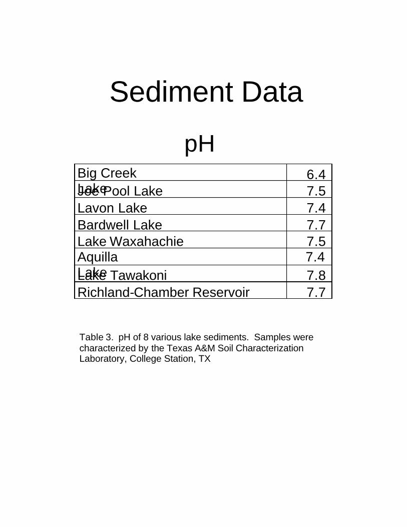
Sediment Data

pH

7.4

Big Creek Lake

6.4 Joe Pool Lake 7.5 Lavon Lake 7.4 Bardwell Lake 7.7 Lake Waxahachie 7.5 Aquilla Lake Lake Tawakoni 7.8 Richland-Chamber Reservoir 7.7

Table 3. pH of 8 various lake sediments. Samples were characterized by the Texas A&M Soil Characterization Laboratory, College Station, TX

Big Creek

Log C

-1.5 -1.0 -0.5 0.0 0.5

1.0

-0.4

-0.2

0.0

0.2

0.4

0.6

0.8

1.0

Graph 1. Graphical representation of the Freundlich equation.

Log X/M

Waxahachie

Log C

-1.5 -1.0 -0.5 0.0 0.5 1.0 -0.4

-0.2

0.0

0.2

0.4

0.6

0.8

1.0


Log X/M

Richland Chambers

Log C -1.5 -1.0 -0.5 0.0 0.5 1.0

-0.4

-0.2

0.0

0.2

0.4

0.6

0.8

1.0


Log X/M

Aquilla

Log C -1.5 -1.0 -0.5 0.0 0.

5 1.0

-0.4

-0.2

0.0

0.2

0.4

0.6

0.8

1.0


Log X/M

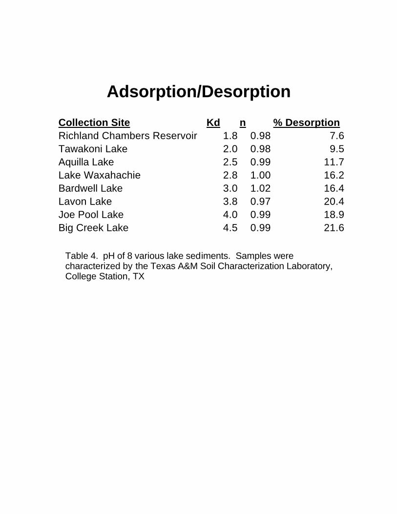
Adsorption/Desorption

Collection Site Kd n % Desorption Richland Chambers Reservoir 1.8 0.98 7.6 Tawakoni Lake 2.0 0.98 9.5 Aquilla Lake 2.5 0.99 11.7 Lake Waxahachie 2.8 1.00 16.2 Bardwell Lake 3.0 1.02 16.4 Lavon Lake 3.8 0.97 20.4 Joe Pool Lake 4.0 0.99 18.9 Big Creek Lake 4.5 0.99 21.6

Table 4. pH of 8 various lake sediments. Samples were characterized by the Texas A&M Soil Characterization Laboratory, College Station, TX

Kd vs. % Desorption

Kd 1.5 2.0 2.5 3.0 3.5 4.0 4.5 5.0

6 8

10

12

14

16

18

20

22

24 %

Desorption

Graph 5. Relationship between Kd and % Desorption.

Literature Cited Ahrens, W.H., 2002. Herbicide handbook. 8th ed. p 27. Weed Sci. Soc. Am.

Champaign, IL. Armstrong, D.E., C. Chesters, and R.F. Harris. 1967. Atrazine hydrolysis in soil. Soil

Sci. Sco. Am. Proc. 31:61-66.

Basta, N.T., R.L. Huhnke, and J.H. Stiegler. 1997. Atrazine runoff from conservation tillage systems: a simulated rainfall study. J. Soil and Water Cons. 52:44-48.

Clay, S.A., W.C. Koskinen. 1990. Adsorption and Desorption of Atrazine,

Hydroxyatrazine, and S-Glutathiioone Atrazine on Two Soils. Weed Science. 38:262-266.

Gao, J.P., J. Maguhn, P. Spitzauer, and A. Kettrup. 1998. Sorption of persticides in the sediment of the Teufelsweiher poond (southern Germany). I: Equilibrium assessments, effect of organic carbon content and pH. Wat. Res. 32:1662-1672.

Giles, C.H., T.H. MacEwan, S.N. Nakhwa, and D. Smith. 1960. A system of classification of solution adsorption isotherms, and its use in diagnosis of adsorption mechanisms and in measurement of specific surface areas of solids. J. Chem. Soc. 3973.

Hall, J.K. 1974. Erosional losses of s-triazine herbicides. J. Environ. Quality.

3:174-180. Hall, J.K., M. Pawlus, and E.R. Higgins. 1972. Losses of atrazine in runoff water and

soil sediment. J. Environ. Qual. 1:172-176. Jones, T.W., W.M. Kemp, J.C. Stevenson, and J.C. Means. 1982. Degradation of

atrazine in estuarine water/sediment systems and soils. J. Environ. Qual. 11:632-638.

Koskinen, W.C., S.S. Harper. 1990. The Retention Process: Mechanisms. Pesticides in

the soil environment: processes, impacts, and modeling. SSSA Book Series. 2:51-77.

Laird, D.A., P.Y. Yen, W.C. Koskinen, T.R. Steinheimer, and R.H. Dowdy. 1994.

Sorption of atrazine on soil clay components. Environ. Sci. Technol. 28:1054- 1061.

Ma, L., and R.F. Spalding. 1997. Herbicide persistence and mobility in recharge lake watershed in York, Nebraska. J. Environ. Qual. 26:115-125.

Mersie, W., C. Seybold, D. Tierney, and C. McName. 1998. Effect of temperature,

disturbance and incubation time on release and degradation of atrazine in water

columns over two types of sediments. Chemosphere. 36:1867-1881. [NASS] National Agricultural Statistics Service. 2003. Graphs on planted and harvested

U.S. corn and sorghum acres. Available at http://www.usda.gov/nass/aggraphs/crops.htm.

Patakioutas, G. T.A. Albanis. 2002. Adsorption-desorption studies of alachlor,

metolachlor, EPTC, chlorothalonil and pirimiphos-methyl in contrasting soils. Pest Manag Sci. 58:353-362.

Pionke, H.B., and D.W. Glotfelty. 1990. Contamination of groundwater by atrazine and

selected metabolites. Chemosphere. 21:813-822. Rae, J.E., C.S. Cooper, A. Parker, and A. Peter. 1998. Pesticide sorption onto aquifer

sediments. J. Geochemical Exploration. 64:263-276.

Seybold, C.A., and W. Mersie. 1996. Adsorption and desorption of atrazine, deethylatrazine, deisopropylatrazine, hydroxyatrazine, and metolachlor in two soils from Virginia. J. Environ. Qual. 25:1179-1185.

Seybold, C.A., W. Mersie, C. McName, and D. Tierney. 1999. Release of atrazine (14C)

from two undisturbed submerged sediments over a two-year period. J. Environ. Qual. 47: 2156-2162.

Spalding, R.F., D.D. Snow, D.A. Cassada, and M.E. Burbach. 1994. Study of pesticide

occurrence in two closely spaced lakes in northeastern Nebraska. J. Environ. Qual. 23:571-578.

Spalding, R.F., and D.D. Snow. 1989. Stream levels of agrichemicals during a spring

discharge event. Chemosphere. 19:1129-1140. Sonon, L.S. and A.P. Schwab. 1995. Adsorption characteristics of atrazine and alachlor

in Kansas soils. Weed Sci. 43:461-466. [TASS] Texas Agricultural Statistics Service. 2003. Crop production summary with

comparisons. Available at http://www.nass.usda.gov/tx/mcorn.htm. [TNRCC] Texas natural resource conservation commission. 2002. Draft 2002 Texas

water quality inventory and 303(d) list. Available at http://www.tnrcc.state.tx.us/water/quality/02_twqmar/index.html.

Triplett, G.B., B.J. Conner, and W.M. Edwards. 1978. Transport of atrazine and

simazine in runoff from conventional and no-tillage corn. J. Environ. Quality. 7:77-83.

Wauchope, R.D. 1978. The pesticide content of surface water draining from agricultural

fields – a review. J. Environ. Qual. 7:459-465. Weber, J.B., 1970. Mechanism of adsorption of s-triazines by clay colloids and factors

affection plant availability. Residue Reviews. 32:93-130. Wu, T.U., D.L. Correll, and H.E.H. Remenapp. 1983. Herbicide runoff from

experimnetal watersheds. J. Environ. Qual. 12:330-336. [EPA] U.S. Environmental Protection Agency. 2003. Atrazine interim re-registration

eligibility decision. Prevention, pesticides and toxic substances. Ying, G.G. and B. Williams. 2000. Laboratory study on the interaction between

herbicides and sediments in water systems. Environmental Pollution. 107:399-405.

Zhang, X.C., L.D. Norton, and M. Hickman. 1997. Rain pattern and soil moisture

content effects on atrazine and metolachlor losses in runoff. J. Environ. Qual. 26:1539-1547.

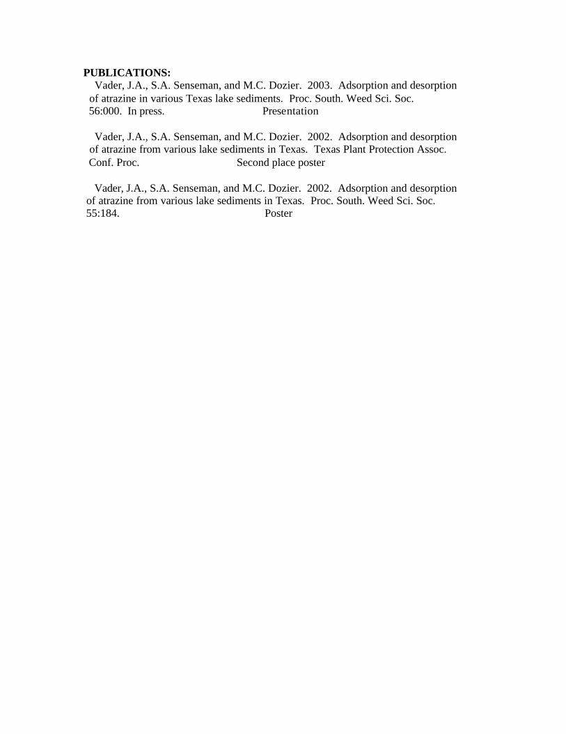
PUBLICATIONS: Vader, J.A., S.A. Senseman, and M.C. Dozier. 2003. Adsorption and desorption of atrazine in various Texas lake sediments. Proc. South. Weed Sci. Soc. 56:000. In press. Presentation Vader, J.A., S.A. Senseman, and M.C. Dozier. 2002. Adsorption and desorption of atrazine from various lake sediments in Texas. Texas Plant Protection Assoc. Conf. Proc. Second place poster Vader, J.A., S.A. Senseman, and M.C. Dozier. 2002. Adsorption and desorption of atrazine from various lake sediments in Texas. Proc. South. Weed Sci. Soc. 55:184. Poster

The Role of Suspended Clays in Phosphrus Processing by Lotic Periphyton

Basic Information

Title: The Role of Suspended Clays in Phosphrus Processing by Lotic Periphyton



End Date: 2/1/2003




Focus Category: Surface Water, Water Quality, Nutrients

Descriptors: None

Principal Investigators: june.e..wolfe.iii.1, Owen T. Lind

Publication

WOLFE - TWRI Graduate Research Enhancement Grant Progress Report March 2002 - February 2003 Project Title: Nutrient processing by in-stream periphyton in a reservoir-

watershed landscape Principle Investigator: Mr. June E. Wolfe, III Co-Principle Investigator: Dr. Owen T. Lind

First Quarter Activity - (March-May 2002):

• Received grant funds and assigned an account number through the Baylor University budget office.

• Ordered supplies – Dionex Ion Chromatograph (IC) Atlas Suppressor. • Became familiar with ion chromatography techniques for

orthophosphate determination in laboratory stream samples. • Became familiar with spectrophotometric techniques for total

phosphorus determination in laboratory stream samples.

Second Quarter Activity - (June-August 2002):

• Ordered supplies – Micro-filtration glassware, filters, and long path equipment for Genesys 5 spectrophotometer.

• Paid student fees for summer seminar course – Basin Watershed Modeling (1 hr).

• Conducted preliminary experiments to develop operating procedures for laboratory streams and determine phosphorus sorption potential of laboratory stream construction materials.

• Developed handling and storage procedures for laboratory stream water samples.

• Developed spreadsheets for data handling.

Third Quarter Activity - (September-November 2002):

• Paid student fees for two courses (Biology Seminar – 1 hr, Interdisciplinary Teaching – 1 hr).

• Logged 1349 travel miles (Temple to Waco and return). • Completed the required Dissertation Research Proposal and filed with

Baylor Biology Department. • Further development of laboratory techniques for phosphorus analysis. • Developed methodologies for determining periphyton biomass.

Fourth Quarter Activity – (December 2002– February 2003)

• Paid student fees for one course (Wetland Ecology – 4 hrs) • Ordered supplies - Polyethylene sample bottles, plastic centrifuge

tubes, high temperature crucibles, chemical reagent. • Requested reimbursement for travel expensed incurred during fall

semester commute. • Became familiar with techniques for measuring clay turbidity in

laboratory streams. • Developed turbidity curves for clays under investigation. • Became familiar with techniques for separating suspended clays from

water samples using a centrifuge. • Evaluated three laboratory stream substrates as phosphorus

sources/sinks.

Information Transfer

Basic Information

Title: Information Transfer



End Date: 2/1/2003




Focus Category: Law, Institutions, and Policy, Management and Planning, Waste Water

Descriptors: None

Principal Investigators: Ric W. Jensen, C. Allan Allan Jones

Publication

1. Gerston, Jan. December 2002. Water and Wastewater Utilities Enhance System Security. TexasWater Resources newsletter.

2. Jensen, Ric. September 2002. TWRI Mills Scholars Program Aids TAMU Graduate Students; Soiland Water Grants Support Research, Extension Efforts, Texas Water Resources newsletter.

3. Jensen, Ric. 2002. New Waves newsletter (3 issues). 4. Alexander, Rachel. 2002. Rio Grande Basin Initiative Outcomes newsletter (2 issues).

Information Transfer Program TWRI 2002

PI: Ricard W. “Ric” Jensen, Ph.D. Articles describing research projects of the Texas Water Resources Institute (TWRI) were publicized in the “Texas Water Resources” and “New Waves” newsletters. These articles presented information about TWRI research to the public in easily understood terms. At the same time, significant efforts were made to describe TWRI research projects on the World Wide Web. This includes a full description of each US Geological Survey (USGS) Project awarded by TWRI and links to popular articles. Special efforts were made to obtain products of funded studies (for example, journal articles, papers, posters, and presentations) and to then make these available to the public. For example, more than 70 special reports and technical reports were web-posted during 2002 that summarize the results of Institute research. TWRI continues efforts to assure the timely communication and dissemination of water resources news via email through the “TWRI WaterTalk” list server. More than 400 people now subscribe to the list server. They are sent 5 messages per day about water resources news, new books and other resources, and meetings and conferences. Significantly, the list server is used to alert researchers and policy makers about opportunities to take part in funding opportunities and to form collaborations for building team partnerships. As a result of publicizing these programs through the list server and Web site, TWRI has significantly increased the number of individuals that apply for competitive grants programs, including those funded by USGS and NIWR. This creates, in turn, more opportunities for collaborative research and extension efforts. More than ever, TWRI is expanding its role to include several research and extension programs supported by external grants. For example, the Institute is working with Texas Cooperative Extension to manage the Rio Grande Basin Initiative, which is funded by the U.S. Department of Agriculture Cooperative State Research Education and Extension Service (USDA/ CSREES). Other significant grants now being administered and publicized by the Institute include projects to market composted dairy manure, efforts to advance hydrologic modeling, and work to investigate the ecological effects of brush control.

In addition to publication and Web site, TWRI has been involved in several meetings, workshops, and conferences. Some of these efforts involve hosting or co-hosting events dealing with bacterial source tracking, the desalination of coastal and inland waters, advances in water related computer modeling, and other topics. Training supported by TWRI included the education of groundwater district managers, and training of small water systems personnel about wellhead protection.

Information Transfer Program

USGS Summer Intern Program

Student Support

Student Support

CategorySection 104Base Grant

Section 104RCGP Award

NIWR-USGS Internship

Supplemental Awards

Total

Undergraduate 3 6 0 0 9

Masters 5 3 0 0 8

Ph.D. 5 0 0 0 5

Post-Doc. 0 0 0 0 0

Total 13 9 0 0 22

Notable Awards and AchievementsJordan Furnans, Ph.D. student at the University of Texas Austin, received a prestigious FullbrightScholarship to help him continue research funded under the USGS 104 program.

Jennifer Hadley, Masters student in Forest Science, Texas A&M University, won the TAMU ViceChancellors award for Teaching in 2003.

Matt Simmons, a Ph.D. graduate student in the department of Rangeland Ecology and Management atTexas A&M University, was asked to present research findings at the Ecological Society of Americaannual conference.

Judy Vader, Masters student in Soil and Crop Sciences, Texas A&M University, won 2nd place at the2003 Texas Plant Protection Society Conference with a poster depicting her USGS based research.

Publications from Prior Projects

texas water resources institute annual technical … water resources institute annual technical...

Documents