text segmentation with topic models - journal for language

Martin Riedl, Chris Biemann

Text Segmentation with Topic Models

This article presents a general method to use information retrieved fromthe Latent Dirichlet Allocation (LDA) topic model for Text Segmentation:Using topic assignments instead of words in two well-known Text Segmenta-tion algorithms, namely TextTiling and C99, leads to significant improve-ments. Further, we introduce our own algorithm called TopicTiling, which isa simplified version of TextTiling (Hearst, 1997). In our study, we evaluateand optimize parameters of LDA and TopicTiling. A further contributionto improve the segmentation accuracy is obtained through stabilizing topicassignments by using information from all LDA inference iterations. Fi-nally, we show that TopicTiling outperforms previous Text Segmentationalgorithms on two widely used datasets, while being computationally lessexpensive than other algorithms.

1 Introduction

Text Segmentation (TS) is concerned with “automatically break[ing] down documentsinto smaller semantically coherent chunks” (Jurafsky and Martin, 2009). We assumethat semantically coherent chunks are also similar in a topical sense. Thus, we view adocument as a sequence of topics. This semantic information can be modeled usingTopic Models (TMs). TS is realized by an algorithm that identifies topical changes inthe sequence of topics.TS is an important task, needed in Natural Language Processing (NLP) tasks, e.g.

information retrieval and text summarization. In information retrieval tasks, TS canbe used to extract segments of the document that are topically interesting. In textsummarization, segmentation results are important to ensure that the summarizationcovers all themes a document contains. Another application could be a writing aid toassist authors with possible positions for subsections.In this article, we use the Latent Dirichlet Allocation (LDA) topic model (Blei

et al., 2003). We show that topic IDs, assigned to each word in the last iterationof the Bayesian inference method of LDA, can be used to improve TS significantlyin comparison to methods using word-based features. This is demonstrated on threealgorithms: TextTiling (Hearst, 1997), C99 (Choi, 2000) and a newly introducedalgorithm called TopicTiling. TopicTiling resembles TextTiling, but is conceptuallysimpler since it does not have to account for the sparsity of word-based features.In a sweep over parameters of LDA and TopicTiling, we find that using topic IDs

of a single last inference iteration leads to enormous instabilities with respect to TSerror rates. These instabilities can be alleviated by two modifications: (i) repeating the

JLCL 2012 – Band 27 (1) – 47-69

Riedl, Biemann

inference iterations several times and selecting the most frequently assigned topic IDfor each word across several inference runs, (ii) storing the topic IDs assigned to eachword for each iteration during the Bayesian inference and selecting most frequentlyassigned topic ID (the mode) per word. Both modifications lead to similar stabilization,however (ii) needs less computational resources. Furthermore, we can also show thatthe standard parameters recommended by Griffiths and Steyvers (2004) do not alwayslead to optimal results.

Using what we have learned in these series of experiments, we evaluate the performanceof an optimized version of TopicTiling on two datasets: The Choi dataset (Choi, 2000)and a more challenging Wall Street Journal (WSJ) corpus provided by Galley et al.(2003). Not only does TopicTiling deliver state-of-the-art segmentation results, italso performs the segmentation in linear time, as opposed to most other recent TSalgorithms.The paper is organized as follows: The next section gives an overview of TS algo-

rithms. Then we introduce the method of replacing words by topic IDs, lay out threealgorithms using these topic IDs in detail, and show improvements for the topic-basedvariants. Section 5 evaluates parameters of LDA in combination with parameters ofour TopicTiling algorithm. In Section 6, we apply the method to various datasets andend with a conclusion and a discussion.

2 Related Work

Topic segmentation can be divided into two sub-fields: (i) linear topic segmentation and(ii) hierarchical topic segmentation. Whereas linear topic segmentation deals with thesequential analysis of topical changes, hierarchical segmentation concerns with findingmore fine grained subtopic structures in texts.

One of the first unsupervised linear topic segmentation algorithms was introduced byHearst (1997): TextTiling segments texts in linear time by calculating the similaritybetween two blocks of words based on the cosine similarity. The calculation is accom-plished by two vectors containing the number of occurring terms of each block. LcSeg,a TextTiling-based algorithm, was published by Galley et al. (2003). In comparisonto TextTiling, it uses tf-idf term weights, which improves TS results. Choi (2000)introduced an algorithm called C99, that uses a matrix-based ranking and a clusteringapproach in order to relate the most similar textual units. Similar to the previousintroduced algorithms, C99 uses words. Utiyama and Isahara (2001) introduced one ofthe first probabilistic approaches using Dynamic Programming (DP) called U00. DP isa paradigm that can be used to efficiently find paths of minimum cost in a graph. TextSegmentation algorithms using DP, represent each possible segment (e.g. every sentenceboundary) as an edge. Providing a cost function that penalizes common vocabularyacross segment boundaries, DP can be applied to find the segments with minimal cost.

Related to our work are a modified C99 algorithm, introduced by Choi et al. (2001)that uses the term-representation matrix in latent space of LSA in combination witha term frequency matrix to calculate the similarity between sentences and two DP

48 JLCL


approaches described in Misra et al. (2009) and Sun et al. (2008): here, topic modelingis used to alleviate the sparsity of word vectors. The algorithm of Sun et al. (2008)follows the approach described in Fragkou et al. (2004), but uses a combination of topicdistributions and term frequencies. A Fisher kernel is used to measure the similaritybetween two blocks, where each block is represented as a sequence of sentences. Thekernel uses a measure that indicates how much topics two blocks share, combinedwith the term frequency, which is weighted by a factor that indicates how likely theterms belong to the same topic. They use entire documents as blocks and generatethe topic model using the test data. This method is evaluated using an artificiallygarbled Chinese corpus. In a similar fashion, Misra et al. (2009) extended the DPalgorithm U00 from Utiyama and Isahara (2001) using topic models. Instead of usingthe probability of word co-occurrences, they use the probability of co-occurring topics.Segments with many different topics have a low topic-probability, which is used as acost function in their DP approach. (Misra et al., 2009) trained the topic model on acollection of the Reuters corpus and a subset of the Choi dataset, and tested on theremaining Choi dataset. The topics for this test set have to be generated for eachpossible segment using Bayesian inference methods, resulting in high computationalcost. In contrast to these previous DP approaches, we present a computationally moreefficient solution. Another approach would be to use an extended topic model thatalso considers segments within documents, as proposed by Du et al. (2010). A furtherapproach for text segmentation is the usage of Hidden Markov Model (HMM), firstintroduced by Mulbregt et al. (1998). Blei and Moreno (2001) introduced an AspectHidden Markov Model (AHMM) which combines an aspect model (Hofmann, 1999)with a HMM. The limiting factor of both approaches is that a segment is assumed tohave only one topic. This problem has been solved by Gruber et al. (2007) who extendsLDA to consider the word and topic ordering using a Markov Chain. In contrast toLDA, not a word is assigned to a topic, but a sentence, so the segmentation can beperformed sentence-wise.

In early TS evaluations, Hearst (1994) measured the fitting of the estimated segmentsusing precision and recall. But these measures are considered inappropriate for the task,since the distance of a falsely estimated boundary to the correct one is not consideredat all. With Pk (Beeferman et al., 1999), a measure was introduced that regulates thisproblem. But there are issues concerning the Pk measure, as it uses an unbalancedpenalizing between false negatives and false positives. WindowDiff (WD) (Pevznerand Hearst, 2002) solves this problem, but most published algorithms still use thePk measure. In practice, both measures are highly correlated. While there are newerpublished metrics (see Georgescul et al. (2006), Lamprier et al. (2007) and Scaiano andInkpen (2012)), in practice still the two metrics Pk and WD are commonly used.

To handle near misses, Pk uses a sliding window with a length of k tokens, which ismoved over the text to calculate the segmentation penalties. This leads to followingpairs: (1, k), (2, k + 1), ..., (n− k, n), with n denoting the length of the document. Foreach pair (i, j) it is checked whether positions i and j belong to the same segment or todifferent segments. This is done separately for the gold standard boundaries and the

JLCL 2012 – Band 27 (1) 49

Riedl, Biemann

estimated segment boundaries. If the gold standard and the estimated segments do notmatch, a penalty of 1 is added. Finally, the error rate is computed by normalizing thepenalty by the number of pairs (n− k), leading to a value between 0 and 1. A valueof 0 denotes a perfect match between the gold standard and the estimated segments.The value of parameter k is assigned to half of the number of tokens in the documentdivided by the number of segments, given by the gold standard.According to Pevzner and Hearst (2002), a drawback of the Pk measure is its

unawareness of the number of segments between the pair (i, j). WD is an enhancementof Pk: the number of segments between position i and j are counted, where again thedistance between the positions is parameterized by k. Then the number of segments iscompared between the gold standard and the estimated segments. If the number ofsegments are not equal, 1 is added to the penalty, which is again normalized by thenumber of pairs to get an error rate between 0 and 1.The first hierarchical algorithm was proposed by Yaari (1997), using the cosine

similarity and agglomerative clustering approaches. A hierarchical Bayesian algorithmbased on LDA is introduced by Eisenstein (2009). In our work, however, we focus onlinear topic segmentation.LDA was introduced by Blei et al. (2003) and is a generative model that discovers

topics based on a training corpus. Model training estimates two distributions: Atopic-word distribution and a topic-document distribution. As LDA is a generativeprobabilistic model, the creation process follows a generative story: First, for eachdocument a topic distribution is sampled. Then, for each document, words are randomlychosen, following the previously sampled topic distribution. Using the Gibbs inferencemethod, LDA is used to apply a trained model for unseen documents. Here, words areannotated by topic IDs by assigning the most probable topic ID on the basis of the twodistributions. Note that the inference procedure, in particular, marks the differencebetween LDA and earlier dimensionality reduction techniques such as Latent SemanticAnalysis.

3 Text Segmentation Datasets

In this paper we use two datasets: A document collection generated based on the Browncorpus and a more challenging corpus generated using WSJ documents.

3.1 Choi Dataset

The Choi dataset (Choi, 2000) is commonly used in the field of TS (see e.g. Misraet al. (2009); Sun et al. (2008); Galley et al. (2003)). It is an artificially generatedcorpus generated from the Brown corpus and consists of 700 documents. Each documentconsists of ten segments. The document generation was performed extracting consecutivesnippets of 3-11 sentences from different documents from the Brown corpus. 400documents consist of segments with a sentence length of 3-11 sentences and there are100 documents each with sentence counts of 3-5, 6-8 and 9-11.

50 JLCL


3.2 Galley Dataset

Galley et al. (2003) present two corpora for written language, each having 500 documents,which are also generated artificially. In comparison to Choi’s dataset, the segmentsin its ’documents’ vary from 4 to 22 segments, and are composed by concatenatingfull source documents. Use of full documents make this corpus a more realistic onein comparison to the one provided by Choi. One dataset is generated based on WSJdocuments of the Penn Treebank (PTB) project (Marcus et al., 1994) and the other isbased on Topic Detection Track (TDT) documents (Wayne, 1998). As the WSJ datasetseems to be harder (consistently higher error rates across several works), we use thisdataset for experimentation.

4 From Words to Topics

4.1 Method to Represent Words with Topic IDs

The method (see also Misra et al., 2009; Sun et al., 2008) for using information gainedby topic models is conceptually simple: Instead of using words directly as features tocharacterize textual units, we use their topic IDs as assigned by Bayesian inference. LDAinference assigns a topic ID to each word in the test document in each inference iterationstep, based on a TM trained on a training corpus. The first series of experiments usethe topic IDs assigned to each word in the last inference iteration. Figure 1 depicts thegeneral setup.

Figure 1: Basic concept of text segmentation using Topic Models

First, preprocessing steps1 like tokenizing, sentence segmentation, part-of-speechtagging or filtering are applied to the training and test documents.

1we use the DKPro framework, http://code.google.com/p/dkpro-core-asl/

JLCL 2012 – Band 27 (1) 51

Riedl, Biemann

The training data used to estimate the topic models should ideally be from the samedomain as the test documents. Since no information about the test data should informthe training, no test documents should be used for the topic model estimation, eventhough topic models belong to the unsupervised learning paradigm. The topic model isestimated once in advance and can then be used for inference on the test documents:LDA inference assigns a topic ID to each word in the test document and generates adocument topic distribution.An example of a text annotated with topic IDs, taken from the WSJ test data, is

presented in Figure 2. One can clearly see the boundary by looking at the most probabletopic IDs. The first text is about a telecommunication company, having mostly topicID 2 assigned to words. The second segment is about an anti-government rally in SouthAfrica. Most words of this segment are annotated with topic ID 37. The topic IDs arenot assigned statically per word, but converge from Gibbs Sampling inference, whichiterates over the words and re-samples topic IDs according to the per-document topicdistribution and the per-topic word probabilities from the previous inference step. Forexample, the word people (marked bold in Figure 2) is marked with topic 37 since thistopic is highly probable in the document. Using this word in a different context wouldmost likely lead to a different topic ID.

Mr:62 .:97 Pohs:2 ,:2 previously:4 executive:2 vice:2 president:2 and:17 chief:2 operating:2officer:2 ,:72 was:2 named:2 interim:2 president:2 and:73 chief:2 executive:2 officer:2 after:17David:2 M:27 .:36 Harrold:65 ,:2 a:84 company:2 founder:2 ,:26 resigned:2 from:91 the:34posts:2 for:62 personal:61 reasons:2 in:84 August:2 .:58 Cellular:70 said:54 Robert:2 J:61.:42 Lunday:2 Jr:18 .:31 ,:44 its:57 chairman:2 and:73 another:25 founder:2 ,:31 resigned:2from:91 the:57 company:2 ’s:24 board:2 to:10 pursue:2 the:10 sale:55 of:67 his:28 telephone:31company:42 ,:74 Big:10 Sandy:50 Telecommunications:31 Inc:2 .:74APARTHEID:37 FOES:37 STAGED:41 a:37 massive:37 anti-government:37 rally:37 in:40South:37 Africa:37 .:19 More:29 than:34 70:45 ,:26 000 people:37 filled:17 a:22 soccer:37stadium:88 on:46 the:34 outskirts:37 of:93 the:24 black:37 township:37 of:45 Soweto:37 and:37welcomed:11 freed:37 leaders:37 of:98 the:57 outlawed:37 African:37 National:45 Congress:87.:72 It:79 was:55 considered:37 South:37 Africa:37 ’s:33 largest:90 opposition:67 rally:37 .:37

Figure 2: Excerpt from a test document, taken from Galley’s WSJ corpus. Each word is followedby a colon and a number, which represents the topic ID.

In the example, all tokens are used for topic model estimation — it is also possibleto filter tokens by parts-of-speech or very short sentences for the purpose of modelestimation and inference. This is expected to lead to even sparser topic distributions.

Once the topic IDs are assigned, most previous segmentation algorithm can be applied,using the topic ID of each word instead of the word itself.In this work, we implement topic-based versions of C99 (Choi, 2000), TextTiling

(Hearst, 1994) and develop a new TextTiling-based method called TopicTiling. Ouraim is to find a simplified algorithm that could solve the segmentation problem usingtopic IDs.

52 JLCL


4.2 Text Segmentation Algorithms using Topic Models

4.2.1 C99 using Topic Models

The topic-based version of the C99 algorithm (Choi, 2000), called C99LDA, dividesthe input text into minimal units on sentence boundaries. A similarity matrix Sm×mis computed, where m denotes the number of units (sentences). Every element sij iscalculated using the cosine similarity (e.g. Manning and Schütze, 1999) between uniti and j. For these calculations, each unit i is represented as a T -dimensional vector,where T denotes the number of topics selected for the topic model. Each element tkof this vector contains the number of times topic ID k occurs in unit i. Next, a rankmatrix R is computed to improve the contrast of S: Each element rij contains thenumber of neighbors of sij that have lower similarity scores then sij itself. This stepincreases the contrast between regions in comparison to matrix S. In a final step, atop-down hierarchical clustering algorithm is performed to split the document into msegments. This algorithm starts with the whole document considered as one segmentand splits off segments until the stop criteria are met, e.g. the number of segments or asimilarity threshold. At this, the ranking matrix is split at indices i, j that maximizethe inside density function D.

D =m∑k=1

sum of ranks within segment karea within segment k (1)

As a threshold-based criterion, the gradient δD is introduced as δD(n) = D(n)−D(n−1).The threshold can then be calculated by µ + c× σ, where mean µ and the standarddeviation σ are calculated from the gradients2.

4.2.2 TextTiling using Topic Models

In TTLDA, the topic-based version of TextTiling (TT) (Hearst, 1994), documents arerepresented as a sequence of n topic IDs instead of words. TTLDA splits the documentinto topic-sequences, instead of sentences, where each sequence consists of w topic IDs.To calculate the similarity between two topic-sequences, called sequence-gap, TTLDAuses k topic-sequences, named block, to the left and to the right of the sequence gap.This parameter k defines the so-called blocksize. The cosine similarity is applied tocompute a similarity score based on the topic frequency vectors of the adjacent blocksat each sequence-gap. A value close to 1 indicates a high similarity among two blocks,a value close to zero denotes a low similarity. Then for each sequence-gap a depth scoredi is calculated for describing the sharpness of a gap, given by

di = 1/2(hl(i)− si + hr(i)− si).

2c = 1.2 as in Choi (2000).

JLCL 2012 – Band 27 (1) 53

Riedl, Biemann

The function hl(i) returns the highest similarity score on the left side of the sequence-gap index i that does not increase and hr(i) returns the highest score on the right side.Then all local maxima positions are searched based on the depth scores.

In the next step, these obtained maxima scores are sorted. If the number of segmentsn is given as input parameter, the n highest depth scores are used, otherwise a cut-offfunction is used that applies a segment only if the depth score is larger than µ− σ/2,where mean µ and the standard deviation σ are calculated based on the entirety ofdepth scores. As TTLDA calculates the depth on every topic-sequence using the highestgap, this could lead to a segmentation in the middle of a sentence. To avoid this, afinal step ensures that the segmentation is positioned at the nearest sentence boundary.

4.2.3 TopicTiling

This section introduces our own Text Segmentation algorithm called TopicTiling whichis based on TextTiling, but conceptually simpler. TopicTiling assumes a sentence sias the smallest basic unit. Between each position p between two adjacent sentences,a coherence score cp is calculated. To calculate the coherence score, we exclusivelyuse the topic IDs assigned to the words by inference: Assuming an LDA model withT topics, each block is represented as a T -dimensional vector. The t-th element ofeach vector contains the frequency of the topic ID t obtained from the respectiveblock. The coherence score is calculated by cosine similarity for each adjacent “topicvector”. Values close to zero indicate marginal relatedness between two adjacent blocks,

0 5 10 15 20 25 30

0.0

0.2

0.4

Sentence

cosi

ne s

imila

rity

Figure 3: Similarity scores plotted for a document. The vertical lines indicate all possible segmentboundaries. The solid lines indicate segments chosen by the threshold criterion, when thenumber of segments is not given in advance.

whereas values close to one denote a substantial connectivity. Next, the coherencescores are plotted to trace the local minima (see Figure 3). These minima are utilizedas possible segmentation boundaries. But rather using the cp values itself, a depth scoredp is calculated for each minimum (cf. TextTiling, Hearst (1997)). In comparison toTopicTiling, TextTiling calculates the depth score for each position and than searchesfor maxima. The depth score measures the deepness of a minimum by looking at thehighest coherence scores on the left and on the right and is calculated using this formula

54 JLCL


(cf. depth score formula in the previous section):

dp = 1/2 ∗ (hl(p)− cp + hr(p)− cp)

The functionality of the function hl (highest peak on the left side) and hr (highestpeak on the right side) is illustrated in Figure 4. The function hl(p) iterates to the

●

●

●

●

●

●

●

●

1 2 3 4 5 6 7 8

0.0

0.4

0.8

1.2

sequence

cohe

renc

e sc

ore

highest right (hr)highest left (hl)

local minimum

Figure 4: Illustration of the highest left and the highest right peak according to a local minimum.

left as long as the score increases and returns the highest coherence score value. Thesame is done, iterating in the other direction with the hr(p) function. According to theillustration, hl(4) = 0.93, the score value at position 2, and hr(4) = 0.99 from the valueat position 7.

If the number of segments n is given as input, the n highest depth scores are used assegment boundaries. Otherwise, a threshold is applied (cf. TextTiling). This thresholdpredicts a segmentation if the depth score is larger than µ − σ/2, with µ being themean and σ being the standard variation calculated on the depth scores.The algorithm runtime is linear in the number of possible segmentation points, i.e.

the number of sentences: for each segmentation point, the two adjacent blocks aresampled separately and combined into the coherence score. This is the main differencesto the dynamic programming approaches for TS described in (Utiyama and Isahara,2001; Misra et al., 2009).

4.3 Experiment: Word-based vs. Topic-based Methods

To show the impact of the topic-based representation introduced in Section 4.1, weshow results for TT and C99 using words and topic IDs, and for TopicTiling.

4.3.1 Experimental Setup

As laid out in Section 4.1, an LDA Model is estimated on a training dataset and usedfor inference on the test set. To ensure that we do not use information from the testset, we perform a 10-fold Cross Validation (CV) for all reported results. To reduce thevariance stemming from the random nature of sampling and inference, the results foreach fold are calculated 30 times using different LDA models.While we aim at not using the same documents for training and testing by using a

folded CV scheme, it is not guaranteed that all testing data is unseen, since the same

JLCL 2012 – Band 27 (1) 55

Riedl, Biemann

source sentences can find their way in several artificially crafted documents. We coulddetect that all sentences from the training subset also occur in the test subset, but notin the same combinations. This makes the Choi data set artificially easy for supervisedapproaches. This problem, however, affects all evaluations on this dataset that use anykind of training, be it LDA models in Misra et al. (2009) or tf-idf values in Fragkouet al. (2004) and Galley et al. (2003).

The LDA model is trained with T = 100 topics, 500 sampling iterations and symmetrichyperparameters as recommended by Griffiths and Steyvers (2004)(α = 50/N andβ = 0.01), using the JGibbsLda implementation of Phan and Nguyen (2007). Unseendata is annotated with topic information, using LDA inference, sampling i = 100iterations. Inference is executed sentence-wise, since sentences form the minimal unitof our segmentation algorithms and we cannot use document information in the testsetting. The performance of the algorithms is measured using Pk and WindowDiff(WD) metrics, cf. Section 2. The C99 algorithm is initialized with a 11×11 rankingmask, as recommended in Choi (2000). TT is configured according to Choi (2000) withsequence length w = 20 and block size k = 6.

4.3.2 Results

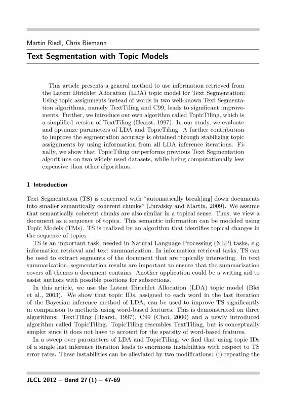
The experiments are executed in two settings using the C99 and TT implementations3:using words (C99, TT) and using topics (C99LDA, TTLDA). TT and C99 use stemmedwords and filter out words using a stopword list. C99 additional removes words usingpredefined regular expressions. In the case of topic-based variants, no stopword filteringor stemming was deemed necessary. Table 1 shows the result of the different algorithmswith segments provided and unprovided.

Method Segments provided Segments unprovidedPk WD Pk WD

C99 11.20 12.07 12.73 14.57C99LDA 4.16 4.89 8.69 10.52TT 44.48 47.11 49.51 66.16TTLDA 1.85 2.10 16.41 21.40TopicTiling 2.65 3.02 4.12 5.75TopicTiling 1.50 1.72 3.24 4.58(filtered)

Table 1: Results by segment length for TT with words and topics (TTLDA), C99 with words andtopics (C99LDA) and TopicTiling using all sentences and using only sentences with morethan 5 word tokens (filtered).

We note that WD values are always higher than the appropriate Pk values. Butwe also observe that these measures are highly correlated. First we discuss resultsfor the setting with number of segments provided (see column 2-3 of Table 1). Asignificant improvement for C99 and TT can be achieved when using topic IDs. In case

3We use the implementations by Choi available at http://code.google.com/p/uima-text-segmenter/.

56 JLCL


of C99LDA, the error rate is at least halved and for TTLDA the error rate is reducedby a factor of 20. The newly introduced algorithm TopicTiling as described above doesnot improve over TTLDA. Analysis revealed that the Choi corpus includes also captionsand other “non-sentences” that are marked as sentences, which causes TopicTilingto introduce false positive segments since the topic vectors are too sparse for theseshort “non-sentences”. We therefore filter out “sentences” with less than 5 words (seebottom line in Table 1). This leads to smaller errors values in comparison to the resultsachieved with TTLDA. Without the number of segments given in advance (see columns3-4 in Table 1), we again observe significantly better results, comparing topic-basedmethods to word-based methods. But the error rates of TTLDA are unexpectedlyhigh. We discovered in data analysis that TTLDA estimates too many segments, asthe topic ID distributions between adjacent sentences within a segment are often toodiverse, especially in face of random fluctuations from the topic assignments. Estimatingthe number of segments is better achieved using TopicTiling instead of TTLDA evenwithout any additional sentence filtering. As we aimed to find a simple algorithm thatcan cope with the topic-based approach, we will use TopicTiling for the next series ofexperiments.

5 Sweeping the Parameter Space of LDA

Aside from the main parameter, the number of topics or dimensions T , surprisingly littleattention has been spent to understand the interactions of hyperparameters, the numberof sampling iterations in model estimation and interference, and the stability of topicassignments across runs using different random seeds in the LDA topic model. Whileprogress in the field of topic modeling is mainly made by adjusting prior distributions(e.g. Sato and Nakagawa, 2010; Wallach et al., 2009), or defining more complex mixturemodels (Heinrich, 2011), it seems unclear whether improvements, reached on intrinsicmeasures like perplexity or on application-based evaluations, are due to an improvedmodel structure or could originate from sub-optimal parameter settings or due to therandomized nature of the sampling process.These subsections address these issues by systematically sweeping the parameter

space and evaluating LDA parameters with respect to text segmentation results achievedby TopicTiling.

5.1 Experimental Setup

Again, the Choi dataset (see Section 3.1) is used, applying a 10-fold CV as described inSection 4.3.1. To assess the robustness of the TM, we sweep over varying configurationsof the LDA model, and plot the results using Box-and-Whiskers plots: the box indicatesthe quartiles and the whiskers are maximally 1.5 times Interquartile Range (IQR) orequal to the data point that has not a distance larger than 1.5 times IQR. The followingparameters are subject to our exploration:

JLCL 2012 – Band 27 (1) 57

Riedl, Biemann

• T : Number of topics used in the LDA model. Common values vary between 50and 500.

• α : Hyperparameter that regulates the sparseness topic-per-document distribution.Lower values result in documents being represented by fewer topics (Heinrich,2004). Recommended: α = 50/T (Griffiths and Steyvers, 2004)

• β : Reducing β increases the sparsity of topics, by assigning fewer terms to eachtopic, which is correlated to how related words need to be, to be assigned to atopic (Heinrich, 2004). Recommended: β = {0.1, 0.01} (Griffiths and Steyvers,2004; Misra et al., 2009)

• mModel estimation iterations. Recommended / common settings: m = 500−5000(Griffiths and Steyvers, 2004; Wallach et al., 2009; Phan and Nguyen, 2007)

• i Inference iterations. Recommended / common settings: 100 (Phan and Nguyen,2007)

• d Mode of topic assignments. At each inference iteration step, a topic ID isassigned to each word within a document (represented as a sentence in ourapplication). With this option (d = true), we count these topic assignmentsfor each single word in each iteration. After all i inference iterations, the mostfrequent topic ID is chosen for each word in a document.

• r Number of inference runs: We repeat the inference r times and assign themost frequently assigned topic per word at the final inference iteration for thesegmentation algorithm. High r values might reduce fluctuations due to therandomized process and lead to a more stable word-to-topic assignment.

• w Window: We introduce a so-called window parameter that specifies the numberof sentences to the left and to the right of position p that define two blocks:sp−w, sp−w+1, . . . , sp and sp+1, . . . , sp+w, sp+w+1.

All introduced parameters parameterize the TM. Other works stabilize topic assignmentsby averaging assignments probed from every 50-100th iteration. Examining this effectmore closely, we look at the mechanisms of using several inference runs r to find thecorrect segments and the mode of topic assignments d. Further, we did not find previouswork that systematically varies TM parameters in combination with measures otherthan perplexity.

5.2 Parameter Sweeping Evaluation

5.2.1 Number of Topics T

To provide a first impression of the data, a 10-fold CV is calculated and the segmentationresults are visualized in Figure 5. Each box plot is generated from the Pk values of 700

58 JLCL


Topic Number

P_k

val

ue

0.0

0.1

0.2

0.3

0.4

0.5

3 10 20 50 100

250

500

●

●

●●

●

●

●

● ● ● ● ●●

●

●● ●●

●●

●●

●

●●

●

●

●

●

●

●

●

●

●

●

●

●

●●

●

●

●

●

●

●

●

●●●

●

●●

●

●

●●

●

●●

●●

●

●●

●

●

●●

●

●

●

●

●

●

●

●

●

●

●●

●

●●

●

●●●

●

●

●●●●●

●

●●●

●

●

●

●

●

●

●

●

●

●

●●

●

●●●

●

●

●

●●●

●

●

Figure 5: Box plots for different number of topics T . Each box plot is generated from the averagePk value of 700 documents, α = 50/T , β = 0.1, m = 1000, i = 100, r = 1.

documents. As expected, there is a continuous range of topic numbers, namely between50 and 150 topics, where we observe the lowest Pk values. Using too many topicsleads to overfitting of the data and too few topics result in too general distinctions tograsp text segment information. This general picture is in line with other studies thatdetermine an optimum for T , (cf. Griffiths and Steyvers, 2004), which is specific tothe application and the data set.

5.2.2 Estimation and Inference iterations

The next step examines the robustness of the model estimation iterations m neededto achieve stable results. 600 documents are used for training an LDA model and theremaining 100 documents are segmented using this model. This evaluation is performedusing 100 topics (as this number leads to stable results according to Figure 5) andperformed using 20 and 250 topics. To assess stability across different model estimationruns, we trained 30 LDA models using different random seeds. Each box plot in Figures6 is generated from 30 mean values, calculated from the Pk values of the 100 documents.The variation indicates the score variance for the 30 different models.

Number of topics: 20

number of sample iterations

P_k

val

ue

0.1

0.2

0.3

0.4

2 3 5 10 20 50 100

300

500

1000

● ● ●●

●●

●

●

●

●

●

●

●

●●

● ● ● ● ● ● ● ● ● ●

●

● ● ●

●

●

●

●●

●● ●● ●

●

●

0.02

0.04

0.06

0.08

0.10

50 100

300

500

1000

●

●

●

●● ● ● ● ● ● ● ● ● ●

●

●

●

●●

●●●

●●

●

●



P_k

val

ue

0.0

0.1

0.2

0.3

0.4

2 3 5 10 20 50 100

300

500

1000

● ● ● ●●

●

●

●

●

●

●

●● ● ● ● ● ● ● ● ● ● ● ● ●

●

●

●

●

●

● ●

0.02

0.04

0.06

0.08

0.10

50 100

300

500

1000

●

●

●

●● ● ● ● ● ● ● ● ● ● ● ●

●

●

● ●



P_k

val

ue

0.1

0.2

0.3

0.4

2 3 5 10 20 50 100

300

500

1000

● ● ● ●●

●

●

●

●

●

●

●●

● ● ● ●●

● ● ●●

● ● ●

●●

●

●

●

●

●

●

●●

●

●

0.02

0.04

0.06

0.08

0.10

50 100

300

500

1000

●

●

●

●● ●

● ●

●

● ● ●●

● ● ●

●

●●

●

●

Figure 6: Box plots with different model estimation iterations m, with T=20,100,250 (from left toright), α = 50/T , β = 0.1, i = 100, r = 1. Each box plot is generated from 30 meanvalues calculated from 100 documents.

JLCL 2012 – Band 27 (1) 59

Riedl, Biemann

Using 100 topics (see Figure 6), the burn-in phase starts with 8–10 iterations andthe mean Pk values stabilize after 40 iterations. But looking at the inset for large mvalues, significant variations between the different models can be observed: note thatthe Pk error rates are between 0.021 - 0.037. As expected using 20 and 250 topicsleads to worse results as with 100 topics. Looking at the plot with 250 topics, a robustrange for the error rates can be found between 20 and 100 sample iterations. Withmore iterations m, the results get both worse and unstable: as the ’natural’ topics ofthe collection have to be split in too many topics in the model, perplexity reductionthat drives the estimation process leads to random fluctuations, which the TopicTilingalgorithm is sensitive to. Manual inspection of models for T = 250 revealed that infact many topics do not stay stable across estimation iterations. In the next step wesweep over several inference iterations i using 100 topics. Starting from 5 iterations,error rates do not change much, see Figure 7a. But there is still substantial variance,between about 0.019 - 0.038 for inference on sentence units.

number of inference iterations

P_k

val

ue

0.01

0.02

0.03

0.04

2 3 5 10 20 50 100

●

●

● ● ● ●● ● ●

●● ●

● ● ●●

●

●

●

●

(a) number of inferences i

number of repeated inferences

P_k

val

ue

0.01

0.02

0.03

0.04

1 3 5 10 20

●

●

●

●

●

●

(b) repeated inference runs r

number of inference iterations

P_k

val

ue

0.01

0.02

0.03

0.04

2 3 5 10 20 50 100

●

●

●●

● ●●

●

●

(c) mode method d = true

Figure 7: Figure a) shows the box plots for different inference iterations i, Figure b) shows the boxplots for several inference runs r and Figure c) presents the usage of the mode methodd = true. All remaining parameters are set to the default values.

5.2.3 Repeat the inference r times

To decrease this variance, we assign the topic not only from a singe inference run, butrepeat the inference calculations several times, denoted by the parameter r. Then thefrequency of assigned topic IDs per token is counted across the r single runs, and weassign the most frequent topic ID (frequency ties are broken randomly). The box plotfor several evaluated values of r is shown in Figure 7b. This log-scaled plot shows thatboth variance and Pk error rate can be substantially decreased. Already for r = 3, weobserve a significant improvement in comparison to the default setting of r = 1 andwith increasing r values, the error rates are reduced even more: for r = 20, variance anderror rates are cut in less than half of their original values using this simple operation.

60 JLCL


5.2.4 Mode of topic assignment d

In the previous experiment, we use the topic IDs that have been assigned most frequentlyat the last inference iteration step. Now, we examine something similar, but for all iinference steps of a single inference run: we select the mode of topic ID assignments foreach word across all inference steps. The impact of this method on error and varianceis illustrated in Figure 7c. Using a single inference iteration, the topic IDs are almostassigned randomly. After 20 inference iterations Pk values below 0.02 are achieved.Using further iterations, the decrease of the error rate is only marginal. In comparisonto the repeated inference method, the additional computational costs of this methodare much lower as the inference iterations have to be carried out anyway in the defaultapplication setting. Note that this is different from using the overall topic distributionas determined by the inference step, since this winner-takes-it-all approach reducesnoise from random fluctuations. As this parameter stabilizes the topic IDs at lowcomputational costs, we recommend using this option in all setups where subsequentsteps rely on single topic assignments.

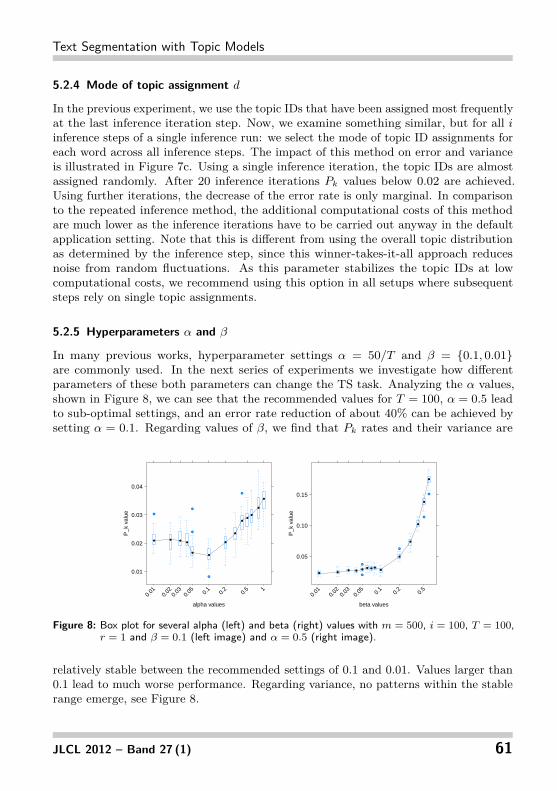
5.2.5 Hyperparameters α and β

In many previous works, hyperparameter settings α = 50/T and β = {0.1, 0.01}are commonly used. In the next series of experiments we investigate how differentparameters of these both parameters can change the TS task. Analyzing the α values,shown in Figure 8, we can see that the recommended values for T = 100, α = 0.5 leadto sub-optimal settings, and an error rate reduction of about 40% can be achieved bysetting α = 0.1. Regarding values of β, we find that Pk rates and their variance are

alpha values

P_k

val

ue

0.01

0.02

0.03

0.04

0.01

0.02

0.03

0.05 0.

10.

20.

5 1

● ● ●●

●●

●

●

●●

●

●

●

●

●

●

●

●

beta values

P_k

val

ue

0.05

0.10

0.15

0.01

0.02

0.03

0.05 0.

10.

20.

5

● ●● ●

●● ● ●

●

●

●

●

●

●

●

●

●

●

●

Figure 8: Box plot for several alpha (left) and beta (right) values with m = 500, i = 100, T = 100,r = 1 and β = 0.1 (left image) and α = 0.5 (right image).

relatively stable between the recommended settings of 0.1 and 0.01. Values larger than0.1 lead to much worse performance. Regarding variance, no patterns within the stablerange emerge, see Figure 8.

JLCL 2012 – Band 27 (1) 61

Riedl, Biemann

5.2.6 Window Parameter w

The optimal window parameter has to be specified according to the documents thatare segmented.

Topic Tiling Window

P_k

mea

sure

0.0

0.1

0.2

0.3

0.4

0.5

1 2 3 4 5 6 7 8 9 10 11 12 13 14 15 16 17 18 19 20 21 22 23 24

● ● ● ● ●●

●●

●

●●

● ● ●

●●

●●

●●

●●

● ●●

●

●●

●

●●

●

●

●

●

●

●

●

●

●●

●●●

●

●

●

●

●

●

●●

●●

●●

●

●

●

●●

●

●●●●

●●

●

●

●

●

●

●

●

●

●

●

●

●●

●

●

●

●

●●

●

●

●

●

●

●

●

●

●●

●

●

●●●

●●

●

●

●●

●

●

●

●

●

●

●

●

●

●

●●

●●

●

●

●

●

●

●

●

●

●

●

●

●

●

●

●

●

●

●

●

●

●

●

●

●

●●

●

●

●

●●

●

●

●

●

●

●●

●

●●

●●

●

●

●

●

●

●●

●●●●●

●

●●

●●

●

●

●

●

●●

●●●●

●

●

●

●●

●

●

●

●●

●

●

●

●

●

●

●

●

●

●●

●

●

●

●

●

●●

●

●

●

●

●

●

●

●●

●

●

●

●

●●

●

●●

●

●●

●●

●

●

●

●

●

●

●

●

●●

●●●

●

●●●●●

●

●●

●

●●●●●

●

●

●

●

●

●

●

●

●

●

●●

●

●

●

●

●

●

●●●●

●●

●

●

●

●

●

●

●

●

●●

●●●

●

●●

●

●

●

●

●

●

●

●●

●●

●

●

●

●●

●

●

●

●

●

●

●

●

●

●

●●

●

●

●

●

●●

●●

●

●●

●

●

●

●

●

●

●

●●

●●●

●

●

●

●

●●

●●

●

●

●●

●● ●

●

●

●

●

●●

●●

●●

●●●

●●

●

●●●

●

●●

●

●

●

●

●

●

●

●

●

●

●

●●

●

●

●

●

●

●

●

● ●●

●

●●

●

●

●

(a) window parameter

0.00 0.01 0.02 0.03 0.04 0.050

5010

015

0P_k values

Den

sity

default valuesalpha=0.01r=20d=truecombined

(b) Error distributions

Figure 9: Figure a) represents the box plots for varying window parameter w with m = 500, i = 100,T = 100, α = 50/T , β = 0.1, r = 1. The Density of the error distribution for the systemaccording to Table 2 is shown in Figure b).

Using the Choi corpus we observe that the window parameter could be increasedto a size of 3 before the error rate increases. Since the segment sizes vary from 3-11sentences we expect a decline for w > 3, which is confirmed by the results shown inFigure 9a.

5.3 Putting it all together

Until this point, we have examined different parameters with respect to stability anderror rates one at the time. Now, we combine what we have learned from this and striveat optimal system performance. Table 2 shows Pk error rates for the different systems.At this, we fixed the following parameters: T = 100, m = 500, i = 100, β = 0.1. For thecomputations we use 600 documents for the LDA model estimation, apply TopicTilingto the 100 remaining documents and repeat this 30 times with different random seeds.

System Pk error σ2 var.red. red.

default 0.0302 0.00% 2.02e-5 0.00%α = 0.1 0.0183 39.53% 1.22e-5 39.77%r = 20 0.0127 57.86% 4.65e-6 76.97%d = true 0.0137 54.62% 3.99e-6 80.21%combined 0.0141 53.45% 9.17e-6 54.55%

Table 2: Comparison of single parameter optimizations, and combined system. Pk averages andvariance are computed over 30 runs, together with reductions relative to the default setting.Default: α = 0.5, r = 1, d = false. combined: α = 0.1, r = 20, d = true

62 JLCL


We observe massive improvements for optimized single parameters. The α-tuningresults in an error rate reduction of 39.77% in comparison to the default configurations.Using r = 20, the error rate is cut in less than half its original value. Also for the modemechanism (d = true) the error rate is halved but slightly worse than when using therepeated inference. Regarding the practice to assign the most frequent topic ID selectedfrom every 50-100th iteration, we conclude that – at least in our application – a muchsmaller number of iterations suffices when taking assignments from all iterations. Here,allowing long inference periods to account for possible topic drifts seems not required.Using combined optimized parameters does not result to additional error decreases. Weattribute the slight decline of the combined method in both the error rate Pk and thevariance to complex parameter interactions that shall be examined in further work. InFigure 9b, we visualize these results in a density plot. It becomes clear that repeatedinference leads to slightly better and more robust performance (higher peak) thanthe mode method. We attribute the difference to situations, where there are severalhighly probable topics in our sampling units, and by chance the same one is picked foradjacent sentences that belong to different segments, resulting in failure to recognizethe segmentation point. However, since the differences are miniscule, only using themode method might be more suitable for practical purposes since its computationalcost is lower.

6 Comparison to other Algorithms

In a last series of experiments, we compare the performance of TopicTiling to otherTS algorithms on several datasets. All LDA models for these series were created usingT = 100, α = 50/T , β = 0.01, m = 500, i = 100.

6.1 Evaluation on the Choi Dataset

The evaluation uses the 10-fold CV setting as described in Section 4.3.1. For thisdataset, no word filtering based on parts of speech was deemed necessary. The resultsfor different parameter settings are listed in Table 3. Using only the window parameter

seg. size 3-5 6-8 9-11 3-11Pk WD Pk WD Pk WD Pk WD

d=false,w=1 2.71 3.00 3.64 4.14 5.90 7.05 3.81 4.32d=true,w=1 3.71 4.16 1.97 2.23 2.42 2.92 2.00 2.30d=false,w=2 1.46 1.51 1.05 1.20 1.13 1.31 1.00 1.15d=true,w=2 1.24 1.27 0.76 0.85 0.56 0.71 0.95 1.08d=false,w=5 2.78 3.04 1.71 2.11 4.47 4.76 3.80 4.46d=true,w=5 2.34 2.65 1.17 1.35 4.39 4.56 3.20 3.54

Table 3: Results based on the Choi dataset with varying parameters.

without the mode (d = false), the results demonstrate a significant error reductionwith a window of 2 sentences. An impairment is observed when using a too large

JLCL 2012 – Band 27 (1) 63

Riedl, Biemann

window (w=5) (cmp. Section 5.2.6). We can also see that the mode method improvesthe results when using a window of 1, except for the documents having small segmentsranging from 3-5 sentences. The lowest error rates are obtained with the mode methodand a window size of 2. As described in Section 4.2.3, the algorithm is also able toautomatically estimate the number of segments using a threshold value (see Table 4).

3-5 6-8 9-11 3-11Pk WD Pk WD Pk WD Pk WD

d=false,w=1 2.39 2.45 4.09 5.85 9.20 15.44 4.87 6.74d=true,w=1 3.54 3.59 1.98 2.57 3.01 5.15 2.04 2.62d=false,w=2 15.53 15.55 0.79 0.88 1.98 3.23 1.03 1.36d=true,w=2 14.65 14.69 0.62 0.62 0.67 0.88 0.66 0.78d=false,w=5 21.47 21.62 16.30 16.30 6.01 6.14 14.31 14.65d=true,w=5 21.57 21.67 17.24 17.24 6.44 6.44 15.51 15.74

Table 4: Results on the Choi dataset without providing the number of segments

As can be seen the optimized parameters leads to worse results for segments of length3-5. This is caused by the smoothing effect of the window parameter which leads toless detected boundaries. But the results of the other documents are comparable to theones shown in Table 3. Some results (see segment length 6-8 and 3-11 with parameterd=true and w=2) are even better than the results with segments provided which isattributed to the remaining variance in the probabilistic inference computations. Thethreshold method can outperform the setup with a given number of segments, sincenot recognizing a segment produces less error in the measures than predicting a wrongsegment. Table 5 presents a comparison of the performance of TopicTiling compared todifferent algorithms in the literature.

Method 3-5 6-8 9-11 3-11TT (Choi, 2000) 44 43 48 46C99 (Choi, 2000) 12 9 9 12U00 (Utiyama and Isahara, 2001) 9 7 5 10LCseg (Galley et al., 2003) 8.69F04 (Fragkou et al., 2004) 5.5 3.0 1.3 7.0M09 (Misra et al., 2009) 2.2 2.3 4.1 2.3TopicTiling (d=true, w=2) 1.24 0.76 0.56 0.95

Table 5: Lowest Pk values for the Choi data set for various algorithms in the literature with providedsegment number.

It is obvious that the results are far better than current state-of-the-art results. Usinga one-sample t-test with α = 0.05 we can state significant improvements in comparisonto all other algorithms. With error rates below the 1% range, TS on the Choi datasetcan be considered as solved. However, since the dataset is comparatively easy, andtest data has probably been seen during model training (cf. Section 4.3), we assess theperformance of our algorithm on a second dataset.

64 JLCL


6.2 Evaluation on Galley’s WSJ Dataset

The evaluation on Galley’s WSJ dataset is performed, using a topic model created fromthe WSJ collection of the PTB. The dataset for model estimation consists of 2499WSJ articles, and is the same dataset Galley used as a source corpus. The evaluationgenerally leads to higher error rates than in the evaluation for the Choi dataset, asshown in Table 6.

Parameters All words FilteredPk WD Pk WD

d=false,w=1 37.31 43.20 37.01 43.26d=true,w=1 35.31 41.27 33.52 39.86d=false,w=2 22.76 28.69 21.35 27.28d=true,w=2 21.79 27.35 19.75 25.42d=false,w=5 14.29 19.89 12.90 18.87d=true,w=5 13.59 19.61 11.89 17.41d=false,w=10 14.08 22.60 14.09 22.22d=true,w=10 13.61 21.00 13.48 20.59

Table 6: Results for Galley’s WSJ dataset using different parameters with using unfiltered documents(column 2-3) and with filtered documents using only verbs, nouns (proper and common)and adjectives (column 3-4).

This table shows results of the WSJ data when using all words of the documentsfor training a topic model and assigning topic IDs to new documents. It also showsresults using only nouns (proper and common), verbs and adjectives4. Considering theunfiltered results, we observe that performance benefits from using the mode assignedtopic ID and a window larger than one. In case of the WSJ dataset, we find the optimalsetting for the window parameter to be 5. As the test documents contain whole articles,which consist of at least 4 sentences, a larger window is advantageous here, yet a valueof 10 is too large. Filtering the documents for parts of speech leads to ∼ 1% absoluteerror rate reduction, as can be seen in the last two columns of Table 6. Again, weobserve that the mode assignment always leads to better results, gaining at least 0.6%.Especially the window size of 5 helps TopicTiling to decrease the error rate to a thirdof the value observed with d=false and w=1. Table 7 shows the results we achieve withthe threshold-based estimation of segment boundaries for the unfiltered and filtereddata.In contrast to the results obtained with the Choi dataset (see Table 4) no decline

occurs, when using the threshold approach in combination with the window method.We attribute this due to the small segments and documents in the Choi dataset. Part-of-speech-based filtering is always advantageous over using all words here. Also a decreaseof both error rates, Pk and WD, is detected when using the mode and using a largerwindow size. An improvement is even gained for a window of size 10. This can beattributed to the fact that using small window sizes, too many boundaries are detected.

4as identified by the Treetagger http://code.google.com/p/tt4j/

JLCL 2012 – Band 27 (1) 65

Riedl, Biemann

Parameters All words FilteredPk WD Pk WD

d=false,w=1 53.07 72.78 52.63 72.66d=true,w=1 53.42 74.12 51.84 72.57d=false,w=2 46.68 65.01 44.81 63.09d=true,w=2 46.08 64.41 43.54 61.18d=false,w=5 30.68 43.73 28.31 40.36d=true,w=5 28.29 38.90 26.96 36.98d=false,w=10 19.93 32.98 18.29 29.29d=true,w=10 17.50 26.36 16.32 24.75

Table 7: Table with results the WSJ dataset without providing the number of segments. Columns2 and 3 show the results when using all words of the documents. Columns 4 and 5 showthe results with part-of-speech-based filtering.

As the window approach smooths the similarity scores, this leads to less segmentationboundaries and improved results.

Table 8 presents the results of other algorithms, as published in Galley et al. (2003),in comparison to TopicTiling. Again, TopicTiling improves over the state of the art.

Method Pk WDC99 Choi (2000) 19.61 26.42U00 Utiyama and Isahara (2001) 15.18 21.54LCseg Galley et al. (2003) 12.21 18.25TopicTiling (d=true,w=5) 11.89 17.41

Table 8: List of results based on the WSJ dataset. Values for C99, U00 and LCseg as stated inGalley et al. (2003).

The improvements with respect to LCseg are significant using a one-sample t-test withα = 0.05.

7 Conclusion

In this article we showed that replacing words in documents by topic IDs, as assigned bythe Bayesian inference method of LDA, leads to better results in the Text Segmentationtask. This technique is applied in the TT and C99 algorithms. Additionally, weintroduced a simplified algorithm based on TT called TopicTiling that outperforms thetopic-based versions of TT and C99. In contrast to other TS algorithms using topicmodels (Misra et al. (2009); Sun et al. (2008)), the runtime of TopicTiling is linearin the number of sentences. This makes TopicTiling a fast algorithm with complexityof O(n) (n denoting the number of sentences) as opposed to O(n2) of the dynamicprogramming approach as discussed in Fragkou et al. (2004).During sweeping the parameter space of LDA and TopicTiling (see Section 5) we

show that repeating the Bayesian inference several times and using the most frequentlyassigned topic IDs in the last iteration not only reduces the variance, but also improves

66 JLCL


overall results. We obtain almost equal performance, when selecting the most frequenttopic ID (mode) assigned per word across each inference step. Although the error ratesare slightly higher in our experiments, this method is preferred, as the computationalcost is much lower than repeating the inference step several times. This method isnot only applicable to Text Segmentation, but in all applications where performancecrucially depends on stable topic ID assignments per token. Using the Choi datasetand the Galleys WSJ dataset we can show significant improved results in comparisonto actual state-of-the-art algorithms.For further work, we would like to devise a method to detect the optimal setting

for the window parameter w automatically, especially in a setting where the numberof target segments is not known in advance. This is an issue that is shared with theoriginal TextTiling algorithm. Moreover, we will extend the usage of our algorithm tomore realistic corpora.

More interesting is the perspective on possible applications. Equipped with a highlyreliable segmentation mechanism, we would like to apply text segmentation as a writingaid to assist authors with feasible segmentation boundaries. This could be applied in aninteractive manner by giving feedback about the coherence during the writing process.As the author is responsible for accepting such segmentation, the need for automaticallydetermining the number of segments would be dispensable, and subject to tuning tothe author’s preferences.Another direction of research that is more generic for approaches based on topic

models is the question of how to automatically select appropriate data for topic modelestimation, given only a small target collection. Since topic model estimation iscomputationally expensive, and topic models for generic collections (think Wikipedia)might not suit the needs of a specialized domain (such as with the WSJ data), it is apromising direction to look at target-domain-driven automatic corpus synthesis.

8 Acknowledgments

This work has been supported by the Hessian research excellence program “Landes-Offensive zur Entwicklung Wissenschaftlich-ökonomischer Exzellenz” (LOEWE) as partof the research center “Digital Humanities”.

References

Beeferman, D., Berger, A., and Lafferty, J. (1999). Statistical models for text segmentation.Machine learning, 34(1):177–210.

Blei, D. M. and Moreno, P. J. (2001). Topic segmentation with an aspect hidden markov model.In Proceedings of the 24th annual international ACM SIGIR conference on Research anddevelopment in information retrieval, SIGIR ’01, pages 343–348, New Orleans, Louisiana,USA.

Blei, D. M., Ng, A. Y., and Jordan, M. I. (2003). Latent Dirichlet Allocation. Journal ofMachine Learning Research, 3:993–1022.

JLCL 2012 – Band 27 (1) 67

Riedl, Biemann

Choi, F. Y. Y. (2000). Advances in domain independent linear text segmentation. In Proceed-ings of the 1st North American chapter of the Association for Computational Linguisticsconference, pages 26–33, Seattle, WA, USA.

Choi, F. Y. Y., Wiemer-Hastings, P., and Moore, J. (2001). Latent semantic analysis for textsegmentation. In Proceedings of EMNLP, pages 109–117, Pittsburgh, PA, USA.

Du, L., Buntine, W., and Jin, H. (2010). A segmented topic model based on the two-parameterpoisson-dirichlet process. Machine Learning, 81(1):5–19.

Eisenstein, J. (2009). Hierarchical text segmentation from multi-scale lexical cohesion. InProceedings of Human Language Technologies: The 2009 Annual Conference of the NorthAmerican Chapter of the Association for Computational Linguistics, pages 353–361, Boulder,CO, USA.

Fragkou, P., Petridis, V., and Kehagias, A. (2004). A Dynamic Programming Algorithm forLinear Text Segmentation. Journal of Intelligent Information Systems, 23(2):179–197.

Galley, M., McKeown, K., Fosler-Lussier, E., and Jing, H. (2003). Discourse segmentation ofmulti-party conversation. In Proceedings of the 41st Annual Meeting on Association forComputational Linguistics, volume 1, pages 562–569, Sapporo, Japan.

Georgescul, M., Clark, A., and Armstrong, S. (2006). An analysis of quantitative aspects in theevaluation of thematic segmentation algorithms. In Proceedings of the 7th SIGdial Workshopon Discourse and Dialogue, pages 144–151, Sydney, Australia.

Griffiths, T. L. and Steyvers, M. (2004). Finding scientific topics. Proceedings of the NationalAcademy of Sciences, 101:5228–5235.

Gruber, A., Rosen-Zvi, M., and Weiss, Y. (2007). Hidden topic markov models. In In Proceedingsof Artificial Intelligence and Statistics, San Juan, Puerto Rico.

Hearst, M. A. (1994). Multi-paragraph segmentation of expository text. In Proceedings of the32nd annual meeting on Association for Computational Linguistics, pages 9–16, Las Cruces,NM, USA.

Hearst, M. A. (1997). TextTiling : Segmenting Text into Multi-paragraph Subtopic Passages.Computational Linguistics, 23(1):33–64.

Heinrich, G. (2004). Parameter estimation for text analysis. Technical report, University ofLeipzig, http://www.arbylon.net/publications/text-est.pdf.

Heinrich, G. (2011). Typology of mixed-membership models: Towards a design method. InMachine Learning and Knowledge Discovery in Databases, volume 6912 of Lecture Notes inComputer Science, pages 32–47. Springer Berlin / Heidelberg. 10.1007/978-3-642-23783-6 3.

Hofmann, T. (1999). Probabilistic Latent Semantic Analysis. In Proceedings of Uncertainty inArtificial Intelligence, UAI’99, pages 289–296, Stockholm, Sweden.

Jurafsky, D. and Martin, J. H. (2009). Speech and Language Processing: An Introduction toNatural Language Processing, Speech Recognition, and Computational Linguistics. PearsonInternational Edition.

68 JLCL


Lamprier, S., Amghar, T., Levrat, B., and Saubion, F. (2007). ClassStruggle. In Proceedingsof the 2007 ACM symposium on Applied computing - SAC ’07, page 600, New York, NewYork, USA. ACM Press.

Manning, C. and Schütze, H. (1999). Foundations of statistical natural language processing.MIT Press, Cambridge, MA.

Marcus, M., Kim, G., Marcinkiewicz, M. A., Macintyre, R., Bies, A., Ferguson, M., Katz, K.,and Schasberger, B. (1994). The Penn Treebank: Annotating predicate argument structure.In Proceedings of the workshop on Human Language Technology, pages 114–119, Plainsboro,NJ, USA.

Misra, H., Yvon, F., Jose, J. M., and Cappe, O. (2009). Text Segmentation via Topic Modeling:An Analytical Study. In Proceeding of the 18th ACM Conference on Information andKnowledge Management, pages 1553–1556, Hong Kong.

Mulbregt, P. v., Carp, I., Gillick, L., Lowe, S., and Yamron, J. (1998). Text segmentation andtopic tracking on broadcast news via a hidden markov model approach. In Proceedings of5th International Conference on Spoken Language Processing, Sydney, Australia.

Pevzner, L. and Hearst, M. A. (2002). A Critique and Improvement of an Evaluation Metricfor Text Segmentation. Computational Linguistics, 28(1):19–36.

Phan, X.-H. and Nguyen, C.-T. (2007). GibbsLDA++: A C/C++ implementation of latentDirichlet allocation (LDA). http://jgibblda.sourceforge.net/.

Sato, I. and Nakagawa, H. (2010). Topic Models with Power-Law Using Pitman-Yor ProcessCategories and Subject Descriptors. Science And Technology, (1):673–681.

Scaiano, M. and Inkpen, D. (2012). Getting more from segmentation evaluation. In ProceedingsConference of North American Chapter of the Association for Computational Linguistics:Human Language Technologies, pages 362–366, Montreal, Canada.

Sun, Q., Li, R., Luo, D., and Wu, X. (2008). Text segmentation with LDA-based Fisher kernel.Proceedings of the 46th Annual Meeting of the Association for Computational Linguisticson Human Language Technologies, pages 269–272.

Utiyama, M. and Isahara, H. (2001). A statistical model for domain-independent text seg-mentation. In Proceedings of the 39th Annual Meeting on Association for ComputationalLinguistics, pages 499–506, Toulouse, France.

Wallach, H., Mimno, D., and McCallum, A. (2009). Rethinking LDA: Why priors matter. InNIPS, Vancouver, B.C., Canada.

Wayne, C. (1998). Topic detection and tracking (TDT): Overview & perspective. In Proceedingsof the Broadcast News Transcription and Understanding Workshop, Lansdowne, Virginia.

Yaari, Y. (1997). Segmentation of expository texts by hierarchical agglomerative clustering. InProceedings of the Conference on Recent Advances in Natural Language Processing, TzigovChark, Bulgaria.

JLCL 2012 – Band 27 (1) 69

text segmentation with topic models - journal for language

Documents