texture and bubble size measurements for modelling
TRANSCRIPT

Texture and Bubble Size Measurements for
Modelling Concentrate Grade
in Flotation Froth Systems
Gordon Forbes
Thesis Presented for the Degree of
DOCTOR OF PHILOSOPHY
in the Department of Chemical Engineering
UNIVERSITY OF CAPE TOWN
August 2007


Synopsis
Numerous machine vision systems for froth flotation have been developed over the last
ten years; however, there are many aspects of the systems that still require further devel-
opment before they become one of the standard instruments present on industrial flotation
operations. This thesis aims to address these problems by developing improved measure-
ment techniques and showing how these measurements can be used to model the concen-
trate grade of the flotation cell being monitored in a manner which is directly usable by
plant personnel.
This thesis presents an improvement to the watershed algorithm for the measurement of
bubble size distributions in flotation froths. Unlike the standard watershed algorithm, it is
able to measure accurate bubble size distributions when both large and tiny bubbles are
present in a flotation froth image.
Flotation froths with “dynamic bubble size distributions” are introduced and methods
of reducing the high dimensional bubble size distribution data associated with them are
discussed. A method of using characteristic histograms of frequently occurring bubble
size distributions is introduced and shown to be an appropriate method to use.
A number of standard texture measures are tested to determine which texture measures
are best suited to the classification of flotation froth images. Results show that the Fourier
ring and texture spectrum based features perform well whilst having a relatively small
computational cost for classifying new images.
Video footage from selected industrial operations has been used for the development of
improved algorithms for the measurement of froth surface descriptors. Analyses of the
relationships between froth velocity, bubble size, froth class and concentrate grade are
i

Synopsis
made. The results show that it is possible to use a unified approach to model the concen-
trate grade, irrespective of the site on which the measurements are made. Results from
three industrial case studies show that bubble size and texture measures can be used to
identify froth classes. Furthermore, the combination of froth class and froth velocity in-
formation is shown to consistently account for the most variation in the data when the
concentrate grade is modelled using a linear combination of these two measurements.
ii

Declaration
I hereby certify that the work embodied in this thesis is the result of original research and
has not been submitted for another degree at any other university or institution.
Gordon Forbes
February 2007
iii

iv

Acknowledgements
I would like to thank the following for their invaluable assistance:
• My supervisors, Dee Bradshaw, Gerhard de Jager and Fred Nicolls for their support
and encouragement.
• The Department of Labour, the National Research Foundation and the Department
of Chemical Engineering at UCT for their financial support of this research project.
Opinions expressed and conclusions arrived at in this thesis are those of the author
and are not necessarily to be attributed to the National Research Foundation.
• Sandy Lambert (Anglo Platinum) and Ray Shaw (Rio Tinto) for funding this
project.
• Bernard Oostendorp, Doug Hatfield and the staff at the Amandelbult UG2 concen-
trator for their assistance during the platinum test work.
• Sameer Morar, Howard Markham and the staff at the Kennecott Utah Copper Con-
centrator for their assistance during the 2004 copper test work.
• The staff at the Kennecott Utah Copper Concentrator for their assistance during the
2006 copper and molybdenum test work.
• Liza Forbes for her assistance during the 2006 copper and molybdenum test work,
help with proof reading and unending love and support.
v

vi

Publications
Peer reviewed conference papers:G. Forbes and G. de Jager. Texture measures for improved watershed segmentation of
froth images. In Fifteenth Annual Symposium of the Pattern Recognition Association ofSouth Africa, pages 1–6, Grabouw, 2004.
G. Forbes and G. de Jager. Bubble size distributions for froth classification. In SixteenthAnnual Symposium of the Pattern Recognition Association of South Africa, pages 99–104,
Langebaan, South Africa, 2005.
G. Forbes, G. de Jager, and D. J. Bradshaw. Effective use of bubble size distribution
measurements. In XXIII International Mineral Processing Congress, pages 554–559,
Istanbul, Turkey, 2006.
G. Forbes and G. de Jager. Unsupervised classification of dynamic froths. In Proceedingsof the Seventeenth Annual Symposium of the Pattern Recognition Association of SouthAfrica, pages 189 – 194, Parys, South Africa, 2006.
Peer reviewed journal papers:G. Forbes and G. de Jager. Unsupervised classification of dynamic froths. Accepted for
pubilcation in SAIEE Africa Research Journal, 2007
Patents:G. Forbes and G. de Jager. A method of determining the size distribution of bubbles in
the froth in a froth flotation process,"SmartFroth 5", Adams & Adams Patent Attorneys
Pretoria A&A REF: 2006/01520. Date of Filing 21 February 2006.
vii

viii

Contents
1 Introduction 1
1.1 Application in Industry . . . . . . . . . . . . . . . . . . . . . . . . . . . 2
1.2 Current System Limitations . . . . . . . . . . . . . . . . . . . . . . . . . 2
1.3 Objectives . . . . . . . . . . . . . . . . . . . . . . . . . . . . . . . . . . 3
1.4 Scope . . . . . . . . . . . . . . . . . . . . . . . . . . . . . . . . . . . . 4
1.4.1 Research areas not addressed . . . . . . . . . . . . . . . . . . . . 6
1.4.1.1 Fundamental Interactions . . . . . . . . . . . . . . . . 6
1.4.1.2 Froth Recovery . . . . . . . . . . . . . . . . . . . . . 6
1.4.1.3 Ore Characteristics . . . . . . . . . . . . . . . . . . . 6
1.4.1.4 Non-linear Models . . . . . . . . . . . . . . . . . . . . 7
1.4.1.5 Froth Colour . . . . . . . . . . . . . . . . . . . . . . . 7
1.4.1.6 Flotation Control . . . . . . . . . . . . . . . . . . . . 7
1.4.1.7 Industrial System . . . . . . . . . . . . . . . . . . . . 7
1.5 Overview of Layout . . . . . . . . . . . . . . . . . . . . . . . . . . . . . 8
2 Literature Review 11
ix

Contents
2.1 Froth Flotation . . . . . . . . . . . . . . . . . . . . . . . . . . . . . . . 12
2.1.1 Grinding Circuit . . . . . . . . . . . . . . . . . . . . . . . . . . 12
2.1.2 Flotation Circuit . . . . . . . . . . . . . . . . . . . . . . . . . . 12
2.1.3 Flotation Control . . . . . . . . . . . . . . . . . . . . . . . . . . 17
2.2 Advantages of Machine Vision Systems . . . . . . . . . . . . . . . . . . 18
2.3 Machine Vision for Flotation Control . . . . . . . . . . . . . . . . . . . . 19
2.3.1 Expert Systems . . . . . . . . . . . . . . . . . . . . . . . . . . . 19
2.3.2 Mass Flow Rate Control . . . . . . . . . . . . . . . . . . . . . . 20
2.3.3 Concentrate Grade Prediction . . . . . . . . . . . . . . . . . . . 20
2.4 Texture Measures for Flotation Froths . . . . . . . . . . . . . . . . . . . 21
2.5 Flotation Froth Bubble Size Measurement . . . . . . . . . . . . . . . . . 22
2.6 Flotation Froth Velocity Measurement . . . . . . . . . . . . . . . . . . . 23
2.7 Machine Vision Measurements & Metallurgical Performance . . . . . . . 25
2.8 Critical Review of Available Literature . . . . . . . . . . . . . . . . . . . 26
2.8.1 Sampling of Video Footage . . . . . . . . . . . . . . . . . . . . 26
2.8.2 Texture . . . . . . . . . . . . . . . . . . . . . . . . . . . . . . . 26
2.8.3 Bubble Size Measurement . . . . . . . . . . . . . . . . . . . . . 27
2.8.4 Velocity . . . . . . . . . . . . . . . . . . . . . . . . . . . . . . . 27
2.8.5 Metallurgical Performance . . . . . . . . . . . . . . . . . . . . . 27
2.9 Objectives . . . . . . . . . . . . . . . . . . . . . . . . . . . . . . . . . . 29
3 Experimental Methodology & Data Sets 31
x
Contents
3.1 Introduction to SmartFroth . . . . . . . . . . . . . . . . . . . . . . . . . 31
3.2 SmartFroth - Hardware . . . . . . . . . . . . . . . . . . . . . . . . . . . 32
3.2.1 Cameras . . . . . . . . . . . . . . . . . . . . . . . . . . . . . . . 33
3.2.2 Zoom and focus settings . . . . . . . . . . . . . . . . . . . . . . 34
3.2.3 Lighting . . . . . . . . . . . . . . . . . . . . . . . . . . . . . . . 34
3.2.4 Camera Mounting and Placement . . . . . . . . . . . . . . . . . 37
3.2.5 Recording Data . . . . . . . . . . . . . . . . . . . . . . . . . . . 40
3.2.6 Calibration . . . . . . . . . . . . . . . . . . . . . . . . . . . . . 40
3.2.7 Computer Requirements . . . . . . . . . . . . . . . . . . . . . . 41
3.3 SmartFroth - Software . . . . . . . . . . . . . . . . . . . . . . . . . . . 41
3.3.1 Colour . . . . . . . . . . . . . . . . . . . . . . . . . . . . . . . 42
3.3.2 Bubble Size . . . . . . . . . . . . . . . . . . . . . . . . . . . . . 42
3.3.2.1 Histogram Equalisation . . . . . . . . . . . . . . . . . 42
3.3.2.2 Low Pass Filtering . . . . . . . . . . . . . . . . . . . . 42
3.3.2.3 Watershed Segmentation . . . . . . . . . . . . . . . . 43
3.3.3 Stability . . . . . . . . . . . . . . . . . . . . . . . . . . . . . . . 47
3.3.4 Velocity . . . . . . . . . . . . . . . . . . . . . . . . . . . . . . . 50
3.3.4.1 Block Matching . . . . . . . . . . . . . . . . . . . . . 50
3.3.4.2 Bubble Tracking . . . . . . . . . . . . . . . . . . . . . 50
3.3.4.3 Stability . . . . . . . . . . . . . . . . . . . . . . . . . 50
3.4 Other Machine Vision Packages for Froth Flotation . . . . . . . . . . . . 52
3.4.1 JK Frothcam . . . . . . . . . . . . . . . . . . . . . . . . . . . . 52
xi

Contents
3.4.2 VisioFroth . . . . . . . . . . . . . . . . . . . . . . . . . . . . . 52
3.4.3 FrothMaster . . . . . . . . . . . . . . . . . . . . . . . . . . . . . 53
3.5 Texture Measures . . . . . . . . . . . . . . . . . . . . . . . . . . . . . . 53
3.5.1 First Order Statistics . . . . . . . . . . . . . . . . . . . . . . . . 54
3.5.2 Greyscale Co-occurrence Matrices . . . . . . . . . . . . . . . . . 56
3.5.3 Fourier Ring/Wedge Filters . . . . . . . . . . . . . . . . . . . . . 57
3.5.4 Gabor Filter Bank . . . . . . . . . . . . . . . . . . . . . . . . . 59
3.5.5 Autoregressive 2D Linear Predictor Model . . . . . . . . . . . . 61
3.5.6 Laws’ Filter Masks . . . . . . . . . . . . . . . . . . . . . . . . . 63
3.5.7 Texture Spectrum . . . . . . . . . . . . . . . . . . . . . . . . . . 64
3.5.8 Wavelets . . . . . . . . . . . . . . . . . . . . . . . . . . . . . . 67
3.6 Classification Methods . . . . . . . . . . . . . . . . . . . . . . . . . . . 69
3.6.1 Geometric Separability Index . . . . . . . . . . . . . . . . . . . 69
3.6.2 KNN Classification . . . . . . . . . . . . . . . . . . . . . . . . . 70
3.6.3 Gaussian Mixture Models . . . . . . . . . . . . . . . . . . . . . 73
3.7 Distribution Distance Measures . . . . . . . . . . . . . . . . . . . . . . . 77
3.7.1 Kolmogorov-Smirnov . . . . . . . . . . . . . . . . . . . . . . . 77
3.7.2 Chi Square . . . . . . . . . . . . . . . . . . . . . . . . . . . . . 77
3.7.3 Cramer / von Mises Distance . . . . . . . . . . . . . . . . . . . . 78
3.7.4 Jeffrey-divergence . . . . . . . . . . . . . . . . . . . . . . . . . 78
3.7.5 Minkowski Distance . . . . . . . . . . . . . . . . . . . . . . . . 78
3.8 Other Techniques . . . . . . . . . . . . . . . . . . . . . . . . . . . . . . 78
xii

Contents
3.8.1 Principal Component Analysis . . . . . . . . . . . . . . . . . . . 79
3.8.2 Unsupervised Classification . . . . . . . . . . . . . . . . . . . . 79
3.9 Introduction to the Data Sets & Froth Classification . . . . . . . . . . . . 83
3.10 Froth Image Data Set . . . . . . . . . . . . . . . . . . . . . . . . . . . . 83
3.11 Discussion on Industrial Data Sets . . . . . . . . . . . . . . . . . . . . . 85
3.11.1 Physical Sampling . . . . . . . . . . . . . . . . . . . . . . . . . 85
3.11.2 Experimental Test Design . . . . . . . . . . . . . . . . . . . . . 85
3.11.3 Number of Data Sets . . . . . . . . . . . . . . . . . . . . . . . . 86
3.11.4 Froth Classes . . . . . . . . . . . . . . . . . . . . . . . . . . . . 87
3.11.5 Identification of Froth Classes . . . . . . . . . . . . . . . . . . . 88
3.12 Platinum Data Set . . . . . . . . . . . . . . . . . . . . . . . . . . . . . . 89
3.12.1 Experimental Setup . . . . . . . . . . . . . . . . . . . . . . . . . 89
3.12.2 Assays . . . . . . . . . . . . . . . . . . . . . . . . . . . . . . . 90
3.12.3 Froth Classes . . . . . . . . . . . . . . . . . . . . . . . . . . . . 90
3.13 Molybdenum Data Set . . . . . . . . . . . . . . . . . . . . . . . . . . . 92
3.13.1 Camera Installation . . . . . . . . . . . . . . . . . . . . . . . . . 92
3.13.2 Process Adjustments . . . . . . . . . . . . . . . . . . . . . . . . 92
3.13.3 Samples . . . . . . . . . . . . . . . . . . . . . . . . . . . . . . . 93
3.13.4 Assays . . . . . . . . . . . . . . . . . . . . . . . . . . . . . . . 94
3.13.5 Froth Classes . . . . . . . . . . . . . . . . . . . . . . . . . . . . 95
3.14 Copper 2004 Data Set . . . . . . . . . . . . . . . . . . . . . . . . . . . . 97
3.14.1 Camera Installation . . . . . . . . . . . . . . . . . . . . . . . . . 97
xiii

Contents
3.14.2 Process Adjustments . . . . . . . . . . . . . . . . . . . . . . . . 97
3.14.3 Samples . . . . . . . . . . . . . . . . . . . . . . . . . . . . . . . 97
3.14.4 Assays . . . . . . . . . . . . . . . . . . . . . . . . . . . . . . . 98
3.14.5 Froth Classes . . . . . . . . . . . . . . . . . . . . . . . . . . . . 98
3.15 Copper 2006 Data Set . . . . . . . . . . . . . . . . . . . . . . . . . . . . 100
3.15.1 Camera Installation . . . . . . . . . . . . . . . . . . . . . . . . . 100
3.15.2 Process Adjustments . . . . . . . . . . . . . . . . . . . . . . . . 100
3.15.3 Sampling . . . . . . . . . . . . . . . . . . . . . . . . . . . . . . 102
3.15.4 Analyses . . . . . . . . . . . . . . . . . . . . . . . . . . . . . . 102
3.15.4.1 Assays . . . . . . . . . . . . . . . . . . . . . . . . . . 102
3.15.4.2 Video Analyses . . . . . . . . . . . . . . . . . . . . . 103
4 Measurement Advances 105
4.1 Improving the Watershed Segmentation Using Texture Measures . . . . . 106
4.1.1 Limitations of the Watershed Algorithm . . . . . . . . . . . . . . 106
4.1.2 Overview of proposed improvement . . . . . . . . . . . . . . . . 109
4.1.3 Classification of Tiny Bubbles . . . . . . . . . . . . . . . . . . . 109
4.1.4 Contrast . . . . . . . . . . . . . . . . . . . . . . . . . . . . . . . 113
4.1.5 Modifying the Watershed . . . . . . . . . . . . . . . . . . . . . . 113
4.1.5.1 First Pass . . . . . . . . . . . . . . . . . . . . . . . . 113
4.1.5.2 Input Image Modification . . . . . . . . . . . . . . . . 115
4.1.5.3 Second Pass . . . . . . . . . . . . . . . . . . . . . . . 115
xiv

Contents
4.1.6 Discussion . . . . . . . . . . . . . . . . . . . . . . . . . . . . . 115
4.2 Reducing BSD Data For Classification . . . . . . . . . . . . . . . . . . . 120
4.2.1 Dynamic Bubble Size Distributions . . . . . . . . . . . . . . . . 120
4.2.2 Testing Methodology . . . . . . . . . . . . . . . . . . . . . . . . 122
4.2.3 Single value descriptors . . . . . . . . . . . . . . . . . . . . . . 123
4.2.4 BSD search . . . . . . . . . . . . . . . . . . . . . . . . . . . . . 127
4.2.5 Aggregate BSDs . . . . . . . . . . . . . . . . . . . . . . . . . . 128
4.2.6 Dimensionality Reduced Aggregate BSD . . . . . . . . . . . . . 130
4.2.7 Frequently Occurring BSDs . . . . . . . . . . . . . . . . . . . . 131
4.2.8 Results . . . . . . . . . . . . . . . . . . . . . . . . . . . . . . . 133
4.2.8.1 Platinum Results . . . . . . . . . . . . . . . . . . . . . 133
4.2.8.2 Copper 2004 Results . . . . . . . . . . . . . . . . . . . 134
4.2.9 Discussion . . . . . . . . . . . . . . . . . . . . . . . . . . . . . 135
4.3 Automatic Learning of Froth Classes . . . . . . . . . . . . . . . . . . . . 137
4.3.1 Algorithm Details . . . . . . . . . . . . . . . . . . . . . . . . . 137
4.3.2 Validation of Results . . . . . . . . . . . . . . . . . . . . . . . . 139
4.4 Texture Measures For Flotation . . . . . . . . . . . . . . . . . . . . . . . 143
4.4.1 Texture Measures Tested . . . . . . . . . . . . . . . . . . . . . . 143
4.4.2 Classification of Froth Images . . . . . . . . . . . . . . . . . . . 145
4.4.3 Results . . . . . . . . . . . . . . . . . . . . . . . . . . . . . . . 145
4.4.4 Discussion . . . . . . . . . . . . . . . . . . . . . . . . . . . . . 146
4.5 Summary of Advances . . . . . . . . . . . . . . . . . . . . . . . . . . . 147
xv

Contents
5 Machine Vision Performance Relationships – Platinum Data Set 149
5.1 Froth Velocity & Concentrate Grade . . . . . . . . . . . . . . . . . . . . 151
5.2 Bubble Size & Concentrate Grade . . . . . . . . . . . . . . . . . . . . . 154
5.3 Froth Class & Concentrate Grade . . . . . . . . . . . . . . . . . . . . . . 158
5.4 Froth Class, Velocity & Concentrate Grade . . . . . . . . . . . . . . . . 161
5.5 Bubble Size, Velocity & Concentrate Grade . . . . . . . . . . . . . . . . 163
5.6 Feed Grade . . . . . . . . . . . . . . . . . . . . . . . . . . . . . . . . . 165
5.7 Summary & Discussion . . . . . . . . . . . . . . . . . . . . . . . . . . . 168
6 Machine Vision Performance Relationships – Molybdenum Data Set 171
6.1 Froth Velocity & Concentrate Grade . . . . . . . . . . . . . . . . . . . . 172
6.2 Bubble Size Measurement . . . . . . . . . . . . . . . . . . . . . . . . . 174
6.2.1 Visible Pulp Areas . . . . . . . . . . . . . . . . . . . . . . . . . 174
6.2.2 Motion Blur . . . . . . . . . . . . . . . . . . . . . . . . . . . . . 175
6.2.3 Transparent Froth . . . . . . . . . . . . . . . . . . . . . . . . . . 176
6.2.4 Poor Segmentation Results . . . . . . . . . . . . . . . . . . . . . 176
6.3 Texture Measures for Froth Identification . . . . . . . . . . . . . . . . . 177
6.4 Froth Class & Concentrate Grade . . . . . . . . . . . . . . . . . . . . . . 179
6.5 Froth Class, Velocity & Concentrate Grade . . . . . . . . . . . . . . . . 182
6.6 Feed versus Froth Class . . . . . . . . . . . . . . . . . . . . . . . . . . . 188
6.7 Process Conditions versus Froth Class . . . . . . . . . . . . . . . . . . . 190
6.8 Summary & Discussion . . . . . . . . . . . . . . . . . . . . . . . . . . . 191
xvi

Contents
7 Machine Vision Performance Relationships – Copper 2006 Data Set 195
7.1 Froth Velocity & Concentrate Grade . . . . . . . . . . . . . . . . . . . . 196
7.2 Bubble Size & Concentrate Grade . . . . . . . . . . . . . . . . . . . . . 199
7.3 Automatic Classification of Froth Classes using Bubble Size Distributions 202
7.4 Froth Class & Concentrate Grade . . . . . . . . . . . . . . . . . . . . . . 207
7.5 Froth Class, Velocity & Concentrate Grade . . . . . . . . . . . . . . . . 210
7.6 Feed versus Froth Class . . . . . . . . . . . . . . . . . . . . . . . . . . . 215
7.7 Process Conditions versus Froth Class . . . . . . . . . . . . . . . . . . . 216
7.8 Summary & Discussion . . . . . . . . . . . . . . . . . . . . . . . . . . . 220
8 Summary, Conclusions & Further Work 223
8.1 Summary . . . . . . . . . . . . . . . . . . . . . . . . . . . . . . . . . . 223
8.1.1 Improved Bubble Size Measurement . . . . . . . . . . . . . . . . 223
8.1.2 Characterisation of Froths with Dynamic BSDs . . . . . . . . . . 224
8.1.3 Texture Measures for Flotation Froths . . . . . . . . . . . . . . . 225
8.1.4 Surface Descriptor - Concentrate Grade Relationships . . . . . . 225
8.1.4.1 Platinum Data Set . . . . . . . . . . . . . . . . . . . . 225
8.1.4.2 Molybdenum Data Set . . . . . . . . . . . . . . . . . . 226
8.1.4.3 Copper 2006 Data Set . . . . . . . . . . . . . . . . . . 227
8.1.5 A Unified Approach . . . . . . . . . . . . . . . . . . . . . . . . 228
8.2 Conclusions . . . . . . . . . . . . . . . . . . . . . . . . . . . . . . . . . 230
8.3 Further Work . . . . . . . . . . . . . . . . . . . . . . . . . . . . . . . . 231
xvii
Contents
8.3.1 Research . . . . . . . . . . . . . . . . . . . . . . . . . . . . . . 231
8.3.1.1 Fundamental Understanding of Froth Classes . . . . . . 231
8.3.1.2 Ore Characteristics . . . . . . . . . . . . . . . . . . . 231
8.3.1.3 Utilising Additional Froth Surface Descriptors . . . . . 231
8.3.1.4 Predictive Capacity . . . . . . . . . . . . . . . . . . . 232
8.3.2 Development . . . . . . . . . . . . . . . . . . . . . . . . . . . . 232
8.3.2.1 Robust Software Implementation . . . . . . . . . . . . 232
8.3.2.2 Robust Hardware Development . . . . . . . . . . . . . 233
8.3.2.3 Implementation of a Machine Vision System . . . . . . 233
8.3.2.4 Machine Vision for Flotation Froth Control . . . . . . . 233
Appendices 235
Bibliography 237
xviii

Acronyms
BSD Bubble Size Distribution
BWS Black-White Symmetry
CBSD Cumulative Bubble Size Distribution
CCTV Closed Circuit Television
CvM Cramer / von Mises
DC Direct Current
DD Degree of Direction
DV Digital Video
GLCM Grey Level Co-occurrence Matrix
GMM Gaussian Mixture Model
GSCOM Grey Scale Co-occurrence Matrix
GS Geometric Symmetry
GSI Geometric Separability Index
KNN K Nearest Neighbour
KS Kolmogorov-Smirnov
LED Light Emitting Diode
MDS Micro-Diagonal Structure
MHS Micro-Horizontal Structure
MLA Mineral Liberation Analyser
MVS Micro-Vertical Structure
PAL Phase Alternating Line
PCA Principal Component Analysis
RMS Root Mean Square
SVHS Super Video Home System
UCT University of Cape Town
VHS Video Home System
xix

xx

Chapter 1
Introduction
Flotation is a separation process used in many mining operations to upgrade the desired
mineral concentration before further downstream processing. The operation of the flota-
tion process is a complex one which is not entirely understood. Each flotation cell has
numerous input parameters (reagent dosage, froth depth, air flow rate) and is also affected
by numerous disturbance variables (ore type, mill performance). Typically, plant opera-
tors inspect the state of the froth visually, taking into account such parameters as velocity,
bubble size, texture, colour and stability. Based on the state of the froth, the operator
might make changes to one or more of the input parameters in order to achieve optimal
performance.
Numerous machine vision systems have been developed since the 1980s with the aim
of improving the control of froth flotation cells. Machine vision systems for froth flota-
tion typically consist of a video camera and light pointing directly at the froth surface.
The video signal is then sent to a computer, which processes the video signal and returns
a variety of measurements. The advantage of having a machine vision system making
measurements of the froth surface is that they are able to produce consistently reliable
measurements that are available 24 hours a day. They also have the potential to pick
up small changes that are not noticeable even by experienced operators. With the ever in-
creasing size of industrial flotation plants, and the limited personnel resources available to
run the flotation plants, having machines which can monitor all of the cells is particularly
useful. Typically measurements made by machine vision systems include froth velocity,
colour, bubble size, texture and stability.
1
Chapter 1: Introduction
1.1 Application in Industry
Despite numerous research projects on the development of such systems, the uptake of
machine vision systems for flotation froth analysis into the minerals processing industry
is slow. Typically, flotation froth machine vision research projects have been performed
using video footage from only one industrial operation, with a limited range of operating
conditions (often the operating conditions used are extreme conditions that do not gener-
ally occur under normal operation). This has resulted in systems which work under the
specific conditions on which they were designed, but do not work well when used on other
concentrators. Experience has shown that although all froth flotation processes are using
the same underlying principles, there is a very large difference in the characteristics of
the froths on different mines. This is generally the result of processing different ore bod-
ies, but is also affected by site specific operating conditions. The result is that numerous
studies which have shown how concentrate grade can be predicted over short time frames
have not been extended to permanent industrial installations, or to other sites.
1.2 Current System Limitations
Typically the research into machine vision systems for flotation froths has been done in
two separate parts. The design and implementation of the measurement algorithms is
typically done by electrical engineers who use a limited amount of video footage that has
been captured from a flotation cell. The video footage is often taken by a metallurgist
working on the mine. The result is that the electrical engineer develops a measurement
based on the limited video footage he has. The methods however, do not scale well to
other froths because they have not been considered by the electrical engineer. When
the system is used on site by metallurgists, they do not understand the limitations of the
system, and poor results are achieved. What is needed from the electrical engineer’s point
of view is to combine the design of the measurements with exposure to the variety of
froths that exist. From the metallurgist’s point of view, there is the need to have at least
some understanding of how the measurements are performed so they will know if the
results are appropriate or not.
2

Chapter 1: Introduction
Experience has shown that the current state of the art algorithms for calculating the bubble
size of flotation froths only work well when a close to uniform bubble size distribution
exists. Poor results are obtained when both large and small bubbles are present. There
is therefore a need to develop advanced algorithms which are capable of providing ac-
curate bubble size measurements for froths with heterogeneous bubble size distributions.
Current methods focus on measuring bubble size distributions for single frames of froth
video footage. However, the existence of froths with “dynamic bubble size distributions”
(froths with rapidly changing bubble size distributions) have been identified and there is
need to formulate an approach that is capable of accurately identifying froth classes under
such dynamic conditions.
Due to the structural behaviour of flotation froths it is not always possible to accurately
measure bubble size distributions. In such cases texture measurements can be used to
describe the froth surface. Some researches have even gone so far as to estimate the bubble
size distribution from texture measurements. Despite numerous researchers using texture
methods for flotation froth classification, there is no current methodology to adequately
compare the variety of texture measures on a suitable data set so as to determine which
texture measures are best suited for the analysis of flotation froths.
1.3 Objectives
This thesis forms part of the University of Cape Town’s collaborative research programme
between the Departments of Electrical and Chemical Engineering to develop a machine
vision instrument for measuring the properties of the visible froth in a flotation cell.
This thesis does not aim to develop such an instrument, but rather to address a sub-set of
the research areas in this larger project. In particular, this thesis aims:
1. To improve bubble size measures by designing an algorithm which is capable of
giving accurate bubble size measurements when both large and tiny bubbles are
present in an image of flotation froth.
2. To determine a methodology for sampling and classifying flotation froths which
exhibit dynamic bubble size distributions.
3

Chapter 1: Introduction
3. To determine which texture measures are best suited to flotation froth imageanalysis by testing a large number of texture measures on a suitably large data base
of flotation froths.
4. To show that relationships exist between machine vision froth surface descrip-tors and the metallurgical performance that can be readily used by industrial
operations to predict the concentrate grade of flotation cells.
5. To show that a unified approach for modelling concentrate grade exists, that
can be systematically applied to industrial flotation operations.
1.4 Scope
In order to achieve these aims, the texture and bubble size measurement have been devel-
oped and tested on a broad range of data from numerous industrial case studies. These
include, a data set from a platinum concentrator that has a flotation froth which has a het-
erogenous bubble size distribution, a data set from a copper concentrator where the froth
typically exhibits a dynamic bubbles size distribution, and a data set from a molybdenum
concentrator for which bubble size measurements do not achieve reliable results and for
which the use of texture measures are appropriate.
For each of these data sets, the appropriate selection of measurement (bubble size, dy-
namic bubble size or texture) is discussed. After the selection of an appropriate measure-
ment, relationships between the measurements, froth velocity and the concentrate grade
of the flotation cell being monitored are presented and discussed.
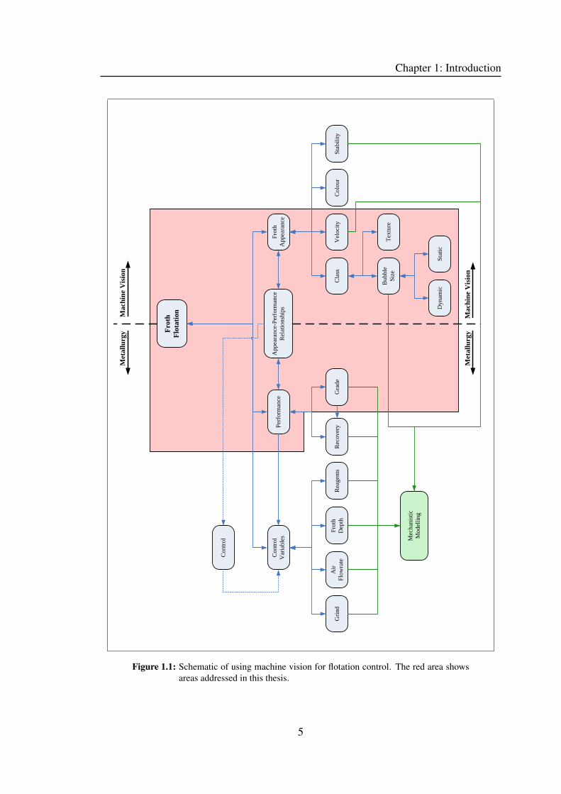
Figure 1.1 shows an overview schematic of using machine vision systems for flotation
control, with the specific areas of work addressed by this thesis indicated in red. These
include the improvement of texture and bubble size measurements and their use in con-
junction with froth velocity measurements for the modelling of the concentrate grade of
the flotation cell being monitored.
4
Chapter 1: Introduction
Perf
orm
ance
Frot
hA
ppea
ranc
e
Cla
ssV
eloc
itySt
abili
tyC
olou
r
Bub
ble
Size
Text
ure
Dyn
amic
Stat
ic
Rea
gent
s
Con
trol
Var
iabl
es
Frot
hD
epth
Air
Flow
rate
Rec
over
yG
rade
App
eara
nce-
Perf
orm
ance
Rel
atio
nshi
ps
Con
trol
Frot
hFl
otat
ion
Met
allu
rgy
Mac
hine
Vis
ion
Met
allu
rgy
Mac
hine
Vis
ion
Grin
d
Mec
hani
stic
Mod
ellin
g
Figure 1.1: Schematic of using machine vision for flotation control. The red area shows
areas addressed in this thesis.
5

Chapter 1: Introduction
1.4.1 Research areas not addressed
As this thesis only deals with a sub-set of a larger research programme, it is important to
state the areas which are within the scope of this thesis and those which are beyond its
scope.
1.4.1.1 Fundamental Interactions
The relationships between the fundamental interactions in the froth phase, pulp phase
and the froth surface descriptors are beyond the scope of this thesis and will not be dealt
with. This is particularly important in light of both the experimental design and the re-
sults presented in this thesis. The focus of this work is the development of appropriate
measurements and demonstrating that a relationship exists between the machine vision
measurements made and the concentrate grade of the flotation cell being measured. The
exact nature of the relationships and their fundamental causes will not be discussed.
1.4.1.2 Froth Recovery
Metallurgical performance of flotation cells is typically specified by the grade and the
recovery of the desired mineral(s). The grade and recovery are related, with their de-
pendency typically being shown on a grade-recovery curve. Improved performance can
typically be achieved by either moving to the desired point on the grade-recovery curve,
or by shifting the entire curve. Shifting the grade-recovery curve is typically achieved
by improving grind / reagent addition. The existence of relationships between the froth
surface descriptors and recovery will not be explored in this thesis.
1.4.1.3 Ore Characteristics
This thesis does not explore the existence of relationships relating the froth surface de-
scriptors to the characteristics of the ore being processed in terms of its grind, mineral
content and liberation. Only the relationship between the froth surface descriptors and
assay grade of the feed is examined.
6

Chapter 1: Introduction
1.4.1.4 Non-linear Models
Numerous non-linear models are used to explain the relationship between the machine
vision froth surface descriptors and the concentrate grade assay values in this work. Due
to the large array of non-linear models available, it was not possible to use all of them.
Non-linear models tested in this work include: 2nd and 3rd order polynomials, power
relationships (axb and axb + c) and exponential relationships (abx and abx + cdx). Fur-
thermore, the use of multiple non-linear regression models falls outside the scope of this
thesis.
1.4.1.5 Froth Colour
The colour of flotation froths and their relationship to metallurgical performance is an area
of ongoing research [45, 32]. Although many publications have shown its usefulness, it is
still difficult to calibrate effectively so that the large number of disturbances are accounted
for. Platinum froths generally look grey, thus making colour analysis inappropriate. The
manner in which this work is performed means that colour analysis of flotation froths can
be easily incorporated into concentrate grade prediction calculations in future work.
1.4.1.6 Flotation Control
The design and implementation of a flotation control system that uses the observed rela-
tionships between froth concentrate grade and the various machine vision froth descriptors
will not be dealt with in this thesis.
1.4.1.7 Industrial System
Although this thesis aims to develop improved bubble size and texture measurements as
well as demonstrate that a relationship exists between the measurements and the concen-
trate grade of the flotation cell being monitored, it does not aim to deliver a stand-alone
piece of equipment that is able to do these tasks in an industrial setting. No hardware
development (camera, lighting, and computer modification) is presented in this thesis.
7

Chapter 1: Introduction
1.5 Overview of Layout
The rest of the thesis is proceeds as follows (Figure 1.2 shows a graphical representation
of the thesis layout):
Introduction[Chapter 1]
Background&
Literature[Chapter 2]
Measurement[Chapter 4]
Results[Chapters 5,6,7]
Discussion&
Conclusions[Chapter 8]
ExperimentalMethodology
[Chapter 3]
Introduction toMachine Vision
In Flotation
Review ofMachine Vision
In Flotation
AlgorithmDetails
SmartFroth Data Sets
Bubble SizeAdvances Texture
PlatinumIndustrial
Data
MolybdenumIndustrial
Data
CopperIndustrial
Data
Figure 1.2: Overview of the thesis layout.
Chapter 2 provides the literature review for the work presented in this thesis. It begins with
an overview of the flotation process. Next it discusses the use of machine vision systems
for improving the performance of flotation cells. A review of the different machine vision
measurement techniques for analysing flotation froths follows. Finally, a critical review
of these methods is made and the objectives of this thesis restated.
Chapter 3 discusses the numerous aspects of experimental procedure used in this work.
It begins by detailing both the hardware and software components of the UCT flotation
froth machine vision system, SmartFroth (the work presented in Chapter 3 is the result of
the research of numerous staff and students at UCT). Next, a technical overview of a large
number of “off-the-shelf” texture algorithms that have been developed is given, followed
by an overview of certain classification algorithms which are used in this thesis and an
overview of numerous distance measures that can be used to calculate the dissimilarity
between bubble size distributions. Finally, the details of the four data sets on which the
results are based are discussed.
Chapter 4 presents novel research which addresses objectives one, two and three. It be-
gins by discussing the limitations of the traditional watershed algorithm. This is followed
by improving the algorithm so that flotation froths which have both large and tiny bubbles
can be successfully segmented. Next, it discusses how to deal with the high dimensional
8

Chapter 1: Introduction
data present in bubble size distributions. Flotation froths with dynamic bubble size dis-
tributions are introduced and ways of classifying them as characteristic histograms of
frequently occurring bubble size distributions are discussed.
The next three chapters address objective number four, presenting results from test work
campaigns. Chapter 5 presents results from an industrial case study on the platinum-
producing Amandelbult UG2 concentrator. Results show that bubble size measurements
can be used to identify froth classes which in turn provide meaningful information on the
metallurgical performance of the flotation cell being monitored.
Chapter 6 presents results from an industrial case study of a flotation cell on the molyb-
denum circuit at the Kennecott Utah Copper Concentrator. Results show how texture
measures can be used to classify froths for which it is not possible to determine accurate
bubble size distributions. The observed relationships between froth class, froth velocity
and metallurgical performance of the flotation cell being monitored are presented. Results
show that the combination of froth velocity and froth class provide valuable information
on the metallurgical performance of the flotation cell being monitored.
In Chapter 7 results are presented for a flotation cell on the copper circuit at the Kennecott
Utah Copper Concentrator. The flotation cell studied had flotation froths with dynamic
bubble size distributions. Froth classes were automatically determined using unsuper-
vised clustering algorithms. Again, the observed relationships between froth class, froth
velocity and metallurgical performance are presented. The combination of froth velocity
and froth class is shown to account for a significant amount of the variability in the data.
Chapter 8 provides a summary of the work that has been performed and a discussion on a
unified approach that can be applied to all three industrial data sets. It ends with a set of
conclusions and suggestions for further work to be done.
9

Chapter 1: Introduction
10
Chapter 2
Literature Review
The aims of this chapter are: to provide a detailed overview of previous research that has
been done on machine vision systems for froth flotations, to provide a critical review of
this research, highlighting specific areas which need further attention, and to present the
set of objectives for this thesis, based on the limitation in the research which has been
done so far.
The chapter begins with a brief overview of the flotation process. Next it describes how
machine vision technology can be used to improve the performance of flotation processes.
After this, a detailed review of the different measurements that have been developed by
various researchers for measuring flotation froth parameters with machine vision systems
are presented. A critical review of this research is presented, indicating areas which re-
quire further input. Key areas of interest include sampling methodologies, texture and
bubble size measurement limitations, and the observed relationships between froth sur-
face descriptors and metallurgical performance. Based on the limitations of the current
research into machine vision systems for froth flotation, a number of objectives for this
thesis are presented.
The critical review and discussion presented in this chapter requires an understanding of
the algorithms on which the measurements of flotation froth systems are made. If the
reader is unfamiliar with these algorithms and techniques, reading Chapter 3 in advance
is advised.
11

Chapter 2: Literature Review
2.1 Froth Flotation
Due to the low head grades of ore being mined (typically 0.5 to 1% for porphyry copper
ores and 1 to 5 ppm for platinum ores), it is necessary to upgrade the concentration of the
desired mineral prior to further processing such as smelting. Froth flotation is a physico-
chemical separation process that is often used in the mining and minerals industry to
remove unwanted waste (gangue) material from the desirable mineral(s).
2.1.1 Grinding Circuit
The process begins with the grinding circuit, where the ore is first crushed, and then milled
to obtain a particle size distribution that is typically sub 100μm. The desired particle size
distribution differs from mine to mine, and is typically a function of the mineralogy of the
ore. The reason for the grinding is to liberate the grains of the desired mineral(s). Water
is added to the mills to transport the ore through the mill and onwards to the classification
section. The mix of ore and water is known as slurry. Closed loop control of the milling
is achieved by using a classification circuit. This is typically achieved using either hydro-
cyclones or a set of screens. Hydro-cyclones are a density separation device, that have
an underflow of coarse particles and an overflow of fine particles. For a screen, the fine
particles pass through the screen, while the coarse particles do not. In both cases, the
coarse particles are fed back to the mill for re-grinding. The fine particles are passed
on to the flotation section. It is not uncommon to have multiple mills, screens and hydro-
cyclones in the grinding circuit. Figure 2.1 shows a typical schematic of a grinding circuit.
2.1.2 Flotation Circuit
Before being pumped into the flotation cells, the slurry typically goes through a set of
conditioning tanks. Various reagents are added to the slurry at the conditioning tanks,
which allow for the time required for the reagents to react with the slurry before the
flotation process begins.
12

Chapter 2: Literature Review
Ball Mill
Rod Mill
Sump
Hydrocyclone
To Flotation
Crusher
Feed
Figure 2.1: Typical grinding circuit diagram.
The slurry is pumped from the conditioning tanks into the first flotation cell. A Flotation
cell is essentially a large tank that contains an impeller to agitate the slurry/air mix, and by
so doing, promote contacting between air bubbles and particles in the slurry. Air spargers
are used to introduce air to the flotation cell. In some flotation cells the rate at which air
is added is fixed, while in other models it is possible to set the air flow rate to a desired
amount.
The agitation from the impeller creates turbulence within the flotation cell. The turbu-
lence in turn promotes particle-bubble collisions. Hydrophobic particles will attach to
the air bubbles, and rise to the surface. The air bubbles form a froth layer on top of
the pulp (slurry). The froth layer overflows the top of the cell into a launder, where the
concentrated material is collected. The upward motion of the air bubbles results in the un-
selective transport of particles to the froth layer in the bubbles’ slipstream. This process
is known as entrainment. Figure 2.2 is a cross section through a flotation cell showing
valuable particles in red and gangue particles in green.
If the froth depth is shallow, it is likely that these entrained particles (most of which are
gangue) will report to the concentrate, lowering the grade. Deeper froth depths have more
time for unattached particles to drain back through the pulp due to gravity. The result is
fewer gangue particles reporting to the concentrate. A level sensor is used to determine
the froth depth, which is controlled in closed loop by varying the flow rate of the pulp
through the tailings outlet.
13

Chapter 2: Literature Review
Figure 2.2: A cross section through a flotation cell (source: Sameer Morar).
Figure 2.3: Three flotation banks on an industrial flotation plant.
14

Chapter 2: Literature Review
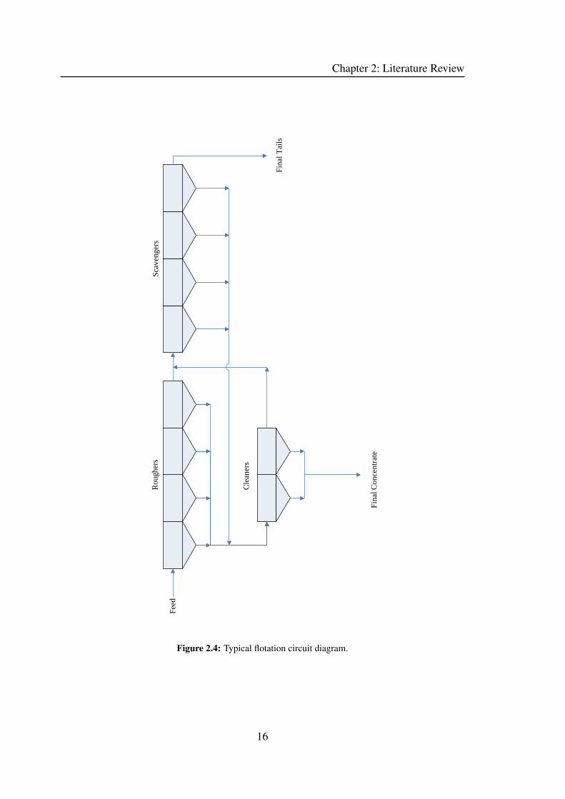
Flotation banks are generally arranged in banks to allow multistage treatment of the slurry,
with recycle loops to ensure that no excess of valuables is lost in the final tailings. Fig-
ure 2.3 shows an industrial flotation bank installation, while Figure 2.4 shows a typical
schematic of a bank of flotation cells.
The chemical state of the pulp in the flotation cell is of utmost importance to ensure that
optimal performance is achieved. Various reagents are added to the pulp for a variety of
reasons:
1. CollectorsThe adsorption of collectors on the surface of minerals renders them hydrophobic
and so enables bubble-particle bonding. It is important for flotation collectors to be
selective so as to not enable flotation of undesired gangue minerals.
2. FrothersFrothers are surface active reagents that interact with the water content of the slurry,
reducing its surface tension. This allows for the formation of thin liquid films that
make up the froth layer. Dosing too little frother will result in an unstable froth
which will collapse, resulting in minimal concentrate being produced. High frother
dosage can result in an overly stable froth, minimising the drainage of entrained
particles and so resulting in lower concentrate grades.
3. ActivatorsActivators are used when the collector will not naturally adsorb onto the mineral
surfaces. Under such circumstances, activators can be used to activate the surface
so that the collector will be able to attach to the desired mineral. It is important to
minimise the inadvertent activation of gangue minerals, as this will result in a lower
grade because they will also report to the concentrate.
4. DepressantsThe adsorption of depressants on the surface of minerals renders them hydrophillic.
Similarly to collectors, depressants are required to be selective so as to prevent the
depression of valuable minerals.
The reagents added to the flotation cell have many competing effects. This means that
it is often particularly difficult to determine the optimal reagent suite for an industrial
flotation plant. Changes in the ore supplied from the mine exacerbate this problem as
ideally different ores should be treated with different reagent suites.
15
Chapter 2: Literature Review
Rou
gher
sSc
aven
gers
Cle
aner
s
Fina
l Tai
ls
Fina
l Con
cent
rate
Feed
Figure 2.4: Typical flotation circuit diagram.
16

Chapter 2: Literature Review
2.1.3 Flotation Control
Despite having been used for over a century, the process of flotation is still not well un-
derstood and is an area of continuing research. Numerous disturbance variables make it
difficult to control a flotation circuit. In particular, the feed to the circuit is constantly
changing in terms of its mass flow rate, mineral composition, level of liberation and par-
ticle size distribution.
On-stream analysers are often used to measure the concentration of various minerals in
slurry streams. This is typically achieved using X-ray diffraction techniques.These ma-
chines tend to be expensive, require extensive maintenance and calibration and are not
able to sample very frequently. As a result, they are used for performance monitoring
rather than closed loop control.
The control of the flotation circuit is traditionally maintained by experience plant person-
nel. These operators visually inspect the state of the froth, and based on their observations,
will make adjustments to one or more of the air flow rate to the cell, the froth depth or
reagent dosage flow rates. Aspects of the froth which the operator will look at include the
froth velocity, colour, bubble size distribution, texture and stability. The disadvantages of
using such a method for control are numerous. Industrial flotation plants keep increasing
in size, while keeping the number of personnel to a minimum. This means that an oper-
ator is not able to continually inspect each flotation cell resulting in a lag time between
when a flotation cell starts to underperform and when the situation is corrected. There is
no guarantee that two operators will make the same decision when the froth of a flotation
cell is in the same state. It is also extremely difficult to determine whether the changes
made by the operator do in fact improve the flotation performance as it is the operator’s
visual inspection which is being used as a performance measure. It is also important to
realise that flotation froths from different ore bodies will look very different, so what may
be a good froth on one flotation plant is not necessarily good for another plant. This
means that operators who are new to a flotation plant will need to learn from others how
the froth looks when the circuit is performing well.
17

Chapter 2: Literature Review
Figure 2.5: Schematic of a typical machine vision system for froth flotation control.
2.2 Advantages of Machine Vision Systems
From the mid-1980s, research groups around the world started projects to see if it would
be possible to use machine vision technology to make appropriate measurements of the
froth surface of a flotation cell using a video camera and machine vision algorithms.
Typically, the signal from the video camera is also recorded onto tapes so that it may be
analysed further at a later stage. A schematic of the typical setup of a machine vision
system is shown in Figure 2.5.
There are a number of distinct advantages of having a machine vision system making
measurements of the froth surface. These include:
1. ConsistencyDifferences in experience levels of individual operators means that there is no guar-
antee that they will have the same opinion of what state the froth is in at any given
time or how best to improve suboptimal conditions. Measurements from a machine
vision system will be consistent across all cells monitored provided that they have
been appropriately calibrated.
2. AvailabilityMachine vision technology is able to provide measurements 24 hours a day. This
is particularly useful considering the large size of modern industrial flotation plants
and the limited number of personnel who operate them.
18

Chapter 2: Literature Review
3. Closed Loop ControlBetter control can be achieved in a closed loop control system. By having consistent
accurate measurements available it is possible to implement closed loop control of
flotation cells. This is not possible when operators make manual adjustments to the
air flow rate, froth depth and reagent dosage levels.
4. Historical DataMachine vision systems can be linked with historian databases. This means that
additional information will be available to determine the cause of faults. It can also
be used to determine optimal condition settings and for training of personnel.
5. High Frequency MeasurementMachine vision systems are able to make high frequency measurements (typically
at 25-30Hz) this means that machine vision systems are able to identify froth states
which have high frequency components which would not be identifiable by an op-
erator. An example of this is the distinguishing of froth states which have dynamic
bubble size distributions (see Section 4.2.1).
2.3 Machine Vision for Flotation Control
Over the years, different approaches have been used by researchers to provide valuable
outputs from machine vision systems for froth flotation control. The next sections discuss
some of the approaches taken.
2.3.1 Expert Systems
Cipriano et al. [11, 12] developed a machine vision system, ACEFLOT, which was used
to provide an expert system with a number of measurements of the froth surface (velocity,
bubble size, colour, stability). The expert system identified certain predefined froth types
when the measurements were in certain ranges. For instance, an excess of lime was indi-
cated by a very slow moving, yellow froth with small bubbles. This could be detected by
the machine vision system by analysing the colour, speed and bubble size measurements.
19
Chapter 2: Literature Review
The expert system gave suggestive corrective actions such as “adjust pH”, but was not
used in closed loop control.
2.3.2 Mass Flow Rate Control
Hatfield and Bradshaw [26] and van Schalkwyk [67] show how machine vision measure-
ments can be used to control the concentrate mass flow rate by adjusting the air flow rate
to the cell on the rougher bank of a platinum concentrator.
2.3.3 Concentrate Grade Prediction
The most common use of machine vision systems found in literature is that of concentrate
grade prediction. There are numerous methods of determining these predictions from the
machine vision systems. Some of the most common approaches in earlier research used
neural networks. These are essentially non-linear models that find a best-fit mapping
between a number of froth surface descriptor inputs and measured concentrate grade out-
puts. More recently, researchers have moved away from the neural network approach
because of it being essentially a “black box”. This is part of the move from characteris-
ing the froth to measuring the froth characteristics [66], a move which has come about
largely due to the limited adoption of machine vision technology on industrial sites. Mea-
surements which directly mimic what operators do when they analyse the froth are better
suited for industrial operations as they are more tangible for plant personnel who would
prefer to not have to deal with complex non-linear models.
The other common technique is to use multiple linear regression of a variety of froth
surface descriptors to determine a model between the descriptors and the concentrate
grade.
Nguyen and Thornton [51] show that texture measures can be used to successfully iden-
tify a variety of froth classes in a coal flotation circuit. They also show that the texture
measures have relationships with the ash and solids content of the froth.
20

Chapter 2: Literature Review
Gorain [19] shows that a linear relationship exists between froth velocity and the con-
centrate grade for a lead flotation circuit as well as a zinc flotation circuit. Kaartinen
and Hyötyniemi [32] show that a combination of stability, colour, speed and bubble size
descriptors can be used to predict the grade of zinc concentrate.
Morar et al. [45] show that the molybdenum, iron and copper grade affect the colour of
the flotation froth. They proceed to show that a linear combination of velocity, stability
and colour measurements can be used to predict copper concentrate grade.
Bartolacci et al. [4] show how various machine vision algorithms can be used to predict
zinc concentrate grade on an industrial flotation plant. They also present results showing
that performance is improved when controlling to a bubble size set point by changing
reagent dosage.
Heinrich [29] showed that a relationship exists between the colour of copper froths and
their concentrate grade. He also proposed a methodology for implementing closed loop
control based on his findings.
Aldrich et al. [1] showed that there were strong correlations between bubble size and
stability measurements with grade and recovery data from a set of batch flotation tests
with varying reagent conditions. The batch tests were performed on a Merensky platinum
ore.
2.4 Texture Measures for Flotation Froths
Numerous texture measures have been used to classify froth images into labelled froth
classes. Moolman et al. [44] show that the Fourier ring texture measurement can be used
to identify different froth classes from an industrial copper operation and that the Fourier
coefficients were related to the bubble size and shape of the flotation froth. Hyötyniemi
and Ylinen [31] and Niemi et al. [52] use the combination of Fourier rings with greyscale
values to identify different froth classes. Their sampling of the froth was at a rate of one
image every 20 seconds. This is not frequent enough to be able to accurately analyse flota-
tion froths with dynamic bubble size distributions, which are introduced later in Section
4.2.1.
21

Chapter 2: Literature Review
Moolman et al. [42] show how both spatial grey level dependence matrices and neighbour-
ing grey level dependence matrices can be used in conjunction with a neural network to
identify five different froth classes from an industrial copper flotation cell. Liu et al. [37]
show that texture features extracted from neighbouring grey level dependence and spatial
grey level dependence matrices appear to be well suited to characterising coal flotation
froths in batch tests.
Nguyen and Thornton [51] introduce the use of the texture spectrum measurement to clas-
sify froths into distinct classes from industrial coal operations. The entire texture spectrum
is used, rather than the reduced set of texture features suggested by He and Wang [28],
because of findings which show no relationship between three texture features and the
identified froth classes [50]. They also show that a nonlinear relationship exists between
the mid_TU peak of the texture spectrum and the bubble size of the flotation froth. The
samples taken were limited to fifty-eight images collected from an entire flotation bank.
This is a small number of images considering the capabilities of video recording equip-
ment. Such a small number of image samples is unlikely to be representative and is also
not able to provide insight into flotation froths with dynamic bubble size distributions.
Bartolacci et al. [4] compare grey level co-occurrence matrix based and wavelet transform
based texture measurements to determine which is best suited for concentrate grade pre-
diction on an industrial zinc operation. The GLCM based methods provide much better
results than the wavelet approach, although both are found to be suited to the task of froth
class identification.
2.5 Flotation Froth Bubble Size Measurement
Guarini et al. [21] describe their method of making bubble size measurements by search-
ing radially at 30◦ intervals for minima. The minima are then joined by elliptical arcs to
identify the individual bubbles. They suggest that the bubble size together with HSI colour
measurements are good froth descriptors, but provide no links between the measurements
and metallurgical performance.
Hargrave, Brown and Hall [23] show that the process conditions can be used to predict
the fractal measurements of the froth structure, and in so doing predict the bubble size
22

Chapter 2: Literature Review
distribution of the froth. This is done to be able to understand how changes in the process
conditions affect the froth structure.
Numerous researchers have worked on using the watershed algorithm for bubble size
measurement of flotation froths [59, 35, 76, 7]. Wright [76] shows that the comparison of
machine vision segmented bubbles to hand segmented bubbles is a difficult task, which
the chi-square test is not suited to: it is possible to have confidence that the segmented im-
ages are both statistically different and statistically the same depending on the bin width
chosen for the bubble size distribution characterisation. Francis [13], discusses various
preprocessing techniques that can be used to improve the results from the bubble segmen-
tation algorithms. These typically take the form of various non-linear filters. Botha [7]
identifies the problem of segmenting flotation froth bubbles which have both large and
tiny bubbles present. He suggested the use of a marker bubble area ratio threshold to
identify areas of fine froth, and acknowledges that there is need for further research into
this area.
Sweet [61] applies the algorithms developed by Wright to both batch and industrial cells.
He shows that different reagent regimes results in different bubble size profiles for batch
flotation tests. Plant test work also showed that the bubble size changes were detectable
by the machine vision system when reagent step changes were made.
Wang et al. [72, 73] present a set of image processing algorithms to determine bubble size
distributions and associated measurements. They initially classify an image based on a
calculation on the white spots of the image, and then proceed to delineate individual bub-
bles using a valley edge detection algorithm. No relationships between the measurements
and metallurgical performance indicators are presented.
2.6 Flotation Froth Velocity Measurement
Moolman et al. [41] develop a method of adding froth velocity information to textural
measures, by modifying the camera such that froths with high velocity appear blurred.
This blurring is in effect a new froth class that can be identified by textural measures.
23

Chapter 2: Literature Review
Nguyen [50] describes the pixel tracing algorithm to measure the velocity of flotation
froths. The algorithm developed by Nguyen is based on the assumption that there is no
distortion between consecutive frames of video. This assumption may well have been
valid for the froths on which Nguyen was working, but does not hold for all flotation
froths, particularly those with dynamic bubble size distributions. The algorithm was de-
signed to be a fast robust measure. However, due to the rapid improvement of computer
technology these limitations are not longer problematic, with the result that more accurate
froth velocity measurements can be made in real time.
Botha et al. [8] describe a method of determining froth velocity by tracking markers from
the watershed between frames of consecutive interlaced video footage. In this manner, a
motion vector field can be created from each bubble in the image, and the average velocity
of the flotation froth can be calculated.
Francis and de Jager [15, 14] describe three methods for measuring the velocity of a
flotation froth: block matching, optical flow and a watershed segmentation based method.
Francis et al. [18] then compare these algorithms to the pixel tracing algorithm used by
Nguyen [50]. Both the optical flow and the block matching algorithms outperform the
pixel tracing method. The watershed based velocity estimate is shown to have the poorest
performance. Francis and de Jager later introduce the Szeliski metric as a method for
comparing motion vector fields in a quantitative manner [16].
Hatfield and Bradshaw [26] show that the watershed based velocity measure is best suited
for specific slow moving froths where its sub-pixel accuracy is desirable. They also show
that it is possible to predict the concentrate mass flow rate using froth velocity measure-
ments. Van Schalkwyk [67] shows how it is possible to control froth velocity by changing
the air flow rate to the cell on an industrial flotation operation.
24

Chapter 2: Literature Review
2.7 Machine Vision Measurements & Metallurgical Per-formance
Cipriano et al. [11] detail the implementation of an expert system which uses bubble size,
colour, froth velocity and froth stability measurements. The expert system identifies in
what state the froth is, and then applies a set of if .. then rules. However, no details are
given for the set of rules that the expert system uses and no metallurgical performance
data is provided.
Kaartinen and Hyötyniemi [32] describe a multi-camera system that uses multivariate
statistical methods on a number of flotation froth surface descriptors (colour, bubble size,
velocity, collapse rate) to predict zinc concentrate grade on an industrial operation. Sam-
pling takes three seconds per cell with only a single frame of footage being used to cal-
culate the bubble size. Whilst these methods may have been appropriate for the flotation
froths analysed in their research, using a single frame to determine bubble size measure-
ments is not suited for all flotation froths, particularly those exhibit dynamic bubble size
distributions (Section 4.2.1).
Moolman et al. [43] show how Sammon maps can be used to reduce the dimensionality
of multi-dimensional texture information. They also show the relationship between the
Sammon map and concentrate grade so that the metallurgical performance of the cell can
be monitored.
Liu et al. [36] use the combination of colour measurements and bubble size distribution
measurements to create a two dimensional process monitoring chart. Test work was per-
formed on an industrial zinc column, and showed that the different steady state conditions
form separate clusters in the process monitoring chart.
Bartolacci et al. [4] show the results of a controller designed to keep the flotation cell at an
optimal bubble size, by changing the CuSO4 addition to the cell. It was found that with
the controller operational, the desired bubble size was achieved for a larger percentage
of time than when it was not operating. From this it is inferred that the performance
25

Chapter 2: Literature Review
of the cell was maximised. The performance improvement was confirmed by anecdotal
evidence provided by plant personnel. No performance data was collected to indicate an
actual improvement. Reagent consumption was reduced by 42% when the controller was
operational.
2.8 Critical Review of Available Literature
2.8.1 Sampling of Video Footage
Within the body of literature relating to machine vision systems for flotation froth there
is a tendency to not publish the exact details of the camera setup. This is specifically
with regard to the number of flotation cells which were used on industrial sites, and the
sampling frequencies and durations. As is seen later in Section 4.2.1 when froths with
dynamic bubble size distributions are introduced, the sampling of the video footage of the
flotation froth is often critical.
The duration of sampling campaigns is also often not reported. It is important to know
how many times a specific froth class was present during a test campaign and if it ap-
peared at numerous times throughout the campaign, or whether it was only present for
one continuous interval. These criteria have a great impact on the validity of the results
of the research, but tend to be neglected.
2.8.2 Texture
Despite many researchers having used texture measurements for froth classification and
concentrate grade prediction, there has up to now not been a comprehensive comparison
of the huge array of texture measures available with an appropriately large data set of
flotation froth images from multiple industrial operations. Such a comparison would be
able to give detailed results on which measurement(s) should be used to classify flotation
froths using texture measures.
26

Chapter 2: Literature Review
2.8.3 Bubble Size Measurement
Despite the improvements in measuring bubble size distributions of flotation froths, there
is still no appropriate method for measuring both large and tiny bubbles in a flotation froth
simultaneously. Research is still required to determine what methods are best suited to
reducing the high dimensionality of bubble size distribution data so that it can be readily
utilised. To overcome the high dimensionality problem, bubble size data is typically re-
duced to either a mean [53, 12, 30, 32], median (p50) or an eightieth percentile (p80)
value. Alternatively, the data is reduced to a set of classes such as small, medium,
large [61]. These reductions are not always appropriate, and can result in the loss of
most of the information contained in a bubble size distribution (see Section 4.2. There is
a need to determine the best way this data reduction can be achieved so as to preserve the
information present in the bubble size distribution.
The sampling of video footage for bubble size distributions is critical for froths which
have rapidly changing bubble size distributions. Despite this requirement, there is no
commentary on the existence of this problem or how to deal with it in the literature on
machine vision systems for flotation froths. Further research is needed to address this
problem.
2.8.4 Velocity
Block matching velocity algorithms provide a robust velocity measure that is suitable for
most flotation froth image analysis scenarios. It is the velocity measure that is used in this
thesis unless specified otherwise.
2.8.5 Metallurgical Performance
Research into predicting metallurgical performance from flotation froth surface descrip-
tors is usually limited by one of the following points: statistical analysis using multiple
linear regression models use large numbers of input variables and quote R2 values as
performance indicators. This is inappropriate as an increasing number of input variables
always results in an improved R2 value. Adjusted R2 values should be used in such cases
27

Chapter 2: Literature Review
as it allows for the meaningful comparison of regression models with differing numbers
of input variables.
When comparing results taken from multiple flotation cells in a bank, such as was done by
Hargrave and Hall [24], it is important to compare them individually in order to observe
trends between metallurgical performance and concentrate grade. There will always be a
natural change in concentrate grade down the bank because the feed to the next cell is the
tailings from the current cell. This means that any observed trends between the flotation
froth descriptors and the concentrate grade are likely to be artificial. Such trends tend
to obscure the desired relationship between metallurgical performance and the individual
cells. It is necessary to be able to identify changes within a single cell if one is to make
any useful predictions from the observed trends.
The repeatability of tests is generally not discussed. Often froth classes are identified, and
algorithms are shown to be able to distinguish between them. However, it is important
for such research, that each froth class has occurred more than once. Ideally they should
have occurred on different days and under different reagent regimes.
Research which uses “black box” approaches such as neural networks (and to a lesser
degree data reduction techniques such as principal component analysis) show some good
results for predicting metallurgical performance. The disadvantage of such techniques
is that the output values are not easy to work with and typically represent no physical
quantity, but are rather simply points in space. This means that although such research
will aid operations by predicting performance, they do not represent easily recognisable
physical qualities. Experience has shown that personnel on industrial operations prefer to
use direct measures of known physical quantities rather than data that has been combined
from many sources in a non-linear manner [66].
Most research on machine vision systems for froth flotation is performed in relative iso-
lation. Due to the vested commercial interest with proprietary machine vision systems,
there are no publicly available data sets of video footage of flotation froths and corre-
sponding metallurgical performance data. This means that each research group works on
a relatively isolated problem with systems being designed with one or two specific flota-
tion froths in mind. This results in systems which work well for certain flotation froths
but poorly for other flotation froths. What is still required is a unified approach which can
be applied to most (if not all flotation froths) with confidence that reliable measurements
28

Chapter 2: Literature Review
will be made. While it is unlikely that such a unified approach can rely on a small set of
measurements, it should be possible to have a systematic approach which can be applied
for the measurement of surface descriptors for most flotation froths, which will ensure
that the appropriate measurements are made for the flotation froth being monitored.
2.9 Objectives
With the comments from the previous section in mind, the specific objectives of this are
restated. This thesis aims:
1. To improve bubble size measures by designing an algorithm which is capable of
giving accurate bubble size measurements when both large and tiny bubbles are
present in an image of flotation froth.
2. To determine a methodology for sampling and classifying flotation froths which
exhibit dynamic bubble size distributions.
3. To determine which texture measures are best suited to flotation froth imageanalysis by testing a large number of texture measures on a suitably large data base
of flotation froths.
4. To show that relationships exist between machine vision froth surface descrip-tors and the metallurgical performance that can be readily used by industrial
operations to predict the concentrate grade of flotation cells.
5. To show that a unified approach for modelling concentrate grade exists, that
can be systematically applied to industrial flotation operations.
29

Chapter 2: Literature Review
30

Chapter 3
Experimental Methodology & Data Sets
This chapter presents the details of the experimental work carried out in this thesis. It be-
gins with an overview of the UCT machine visions system for the analysis flotation froths,
SmartFroth, both in terms of the hardware and software requirements of the system.
Next, a variety of texture measurements are discussed. These texture measures form the
foundation of the texture work presented in Chapter 4 which determines which texture
measures are best suited for the classification of flotation froth images.
Classification methods, measures for the comparison of distributions and other techniques
used in Chapter 4 are presented next. These sections provide the detail of the tests per-
formed in subsequent chapters.
Finally, the data sets used for this thesis are presented. These include: the platinum data
set, two copper data sets, the molybdenum data set and the froth image data set.
3.1 Introduction to SmartFroth
The SmartFroth system forms the foundation on which most of the work presented in this
thesis is based. It is the result of the research of many MSc and PhD students. The Smart-
Froth system is a fully functional machine vision system that can be used to measure a
31

Chapter 3: Experimental Methodology & Data Sets
variety of features relating to the surface of a flotation froth. Despite being a robust use-
able system, there are still many areas where the measurements can be improved so that
they will be more accurate and apply to a greater number of flotation froths. The algo-
rithmic details in presented in this chapter are the prior work of previous UCT students.
In the subsequent chapters, modifications and improvements to the algorithms mentioned
here will be proposed and tested. The improvements to these algorithms presented in the
subsequent chapters form part of the novel contributions of this thesis.
It is important to have at least some understanding of how the measurements are made on
an algorithmic level. This knowledge allows one to understand when a particular measure-
ment will be accurate and when it will not. This is much the same as understanding the
limitations of any measurement device. For example, different thermometers are designed
for different temperature ranges. Also there are different ways of measuring temperature
(alcohol thermometers, mercury thermometers, thermocouples, solid-state integrated cir-
cuits, etc.). Each of these will give temperature measurements for a given substance, but
for the best precision and accuracy there will be an optimal choice for each substance
that has its temperature measure. In much the same way, there are numerous algorithms
and hardware solutions that allow the measurement of various flotation froth descriptors.
However, the choice of algorithm and hardware solution for a given flotation froth can
greatly affect the precision and accuracy of the measurements made.
3.2 SmartFroth - Hardware
At the simplest level, a machine vision system for monitoring flotation froths consists of a
video camera and light mounted above the flotation froth, with the output from the video
camera connected to a computer. Software on the computer then makes measurements on
the images embedded in the video signal it receives. These measurements are then either
displayed for operators to make decisions from or used in a closed loop control system.
Due to the difference in design of flotation cells, it is not easy to ensure that a single piece
of equipment is suited for analysing the flotation froth of any flotation cell in the world.
As such, there is an array of equipment which can be used to set up a machine vision
system to monitor flotation froths. This section will discuss the equipment used in a few
32

Chapter 3: Experimental Methodology & Data Sets
typical installations on concentrators. An important factor in the installation is whether
or not it is going to be a temporary (typically less than two months) installation or a long-
term installation (typically greater than two months). Short-term installations are usually
done when collecting data on a sampling campaign, as they are quicker to set up and take
down when finished.
3.2.1 Cameras
Two main types of cameras are typically used. Standard CCTV Colour board cameras
with an appropriate zoom lens, which is enclosed in a waterproof mounting is typically
used for the long-term installations. These cameras run of a 12V power supply and have a
PAL composite video output. An example of such a video camera is show in Figure 3.1a.
(a) (b)
Figure 3.1: A CCTV board camera with lens and a typical camcorder used for capturing
video sequences of flotation froths.
For short-term installations, digital camcorders are typically used. The output from the
camcorders is either a PAL composite video output, or via the IEEE1394 firewire stan-
dard. An example of a typical camera installation is show in Figure 3.1b.
33

Chapter 3: Experimental Methodology & Data Sets
3.2.2 Zoom and focus settings
The zoom and focus of the CCTV cameras needs to be set up so that the field of view
is appropriately sized and in focus. The zoom level is set such that the largest possible
bubbles take up approximately 20% of the image. It is not possible to determine an
accurate bubble size distribution measurement if the bubble is larger than the field of
view of the camera. Ideally, the smallest bubbles should have an area of a few pixels so
that they too can be identified. Because of this, the setup for each cell will be different.
Typical fields of view vary from 133×100mm to 400×300mm. Figure 3.2 shows two
different fields of view, although the bubble size in the images is approximately the same.
Figure 3.2: Two froth images with different fields of view.
For a digital camcorder, the zoom can be adjusted easily by using the zoom function. The
focus is also adjusted automatically by the camera, but can also be set to manual mode if
desired.
3.2.3 Lighting
Correct illumination of the froth is of the utmost importance. Whether flotation cells are
indoors or outdoors the illumination is generally not suited to the capturing of high quality
images with a video camera. Because of this additional illumination and shielding from
other light sources is usually required. Figures 3.3 and 3.4 show the typical illumination
of froths before additional lighting and shielding have been installed.
34

Chapter 3: Experimental Methodology & Data Sets
Figure 3.3: A poorly illuminated froth with multiple highlights on the froth surface result
in poor bubble size measurement.
Figure 3.4: Patches of sunlight falling onto the field of view of the camera system results
in poor measurements and should be avoided.
35

Chapter 3: Experimental Methodology & Data Sets
Due to the nature of the watershed algorithm (used for the bubble size distribution mea-
surements), it is desirable to have a single highlight on the top of each bubble. See Fig-
ure 3.3 for an example of a poorly illuminated froth and Figure 3.5 for an example of
well illuminated froths with single highlights on each bubble. Since each light used will
create a highlight (unless appropriate diffusing is used), the solution is to use a single high
brightness light. This typically takes the form of a 500W halogen light. The disadvantage
of a 500W halogen light is the heat that is generated. The combination of heat, a sensitive
bulb, vibration of heavy machinery and an often wet environment means that these lights
are not very suitable for long-term installations as the bulbs and glass panes of the lights
often break.
Figure 3.5: Two well illuminated froths. Note the single highlights on each bubble.
An alternative solution has been designed which makes use of a ring of high power LEDs
which are focused on a single point so as to ensure a single highlight on the froth. Since
LEDs run much cooler than 500W halogen lights, the associated problems are overcome.
The ring of LEDs is mounted around the camera. This can be seen in Figure 3.6.
Sometimes it is necessary to use a hood, to shield the froth from external light sources
(typically the sun and overhead lighting). This needs to be done when the lighting used
is not powerful enough to damp out the effect of the external lighting, which results in
multiple highlights on the froth surface. In some partially open concentrators, shadows
and patches of light are sometimes cast across the froth surface. Figures 3.3 and 3.4 shows
examples of such events. It is also important to use a hood to shield the froth from ambient
lighting fluctuations when colour test work is being performed. This however is not dealt
with in this work. An example of a camera with a hood installed is shown in Figure 3.7a.
36

Chapter 3: Experimental Methodology & Data Sets
Figure 3.6: SmartFroth camera in waterproof housing with ring of LEDs for consistent
illumination.
3.2.4 Camera Mounting and Placement
For long-term installations it is usually necessary to have an on site technician construct
some appropriate mounting equipment for the camera, light and hoods. For temporary
installations, both cameras and lights can usually be mounted using articulated arms with
clamps on the end. Figure 3.7 shows two examples of a long-term installation and Fig-
ure 3.8 shows two examples of short-term camera installations.
It is important to mount the camera such that it is observing an area of froth which is
representative of the cell it is monitoring. As such it is best if it is place in a central
area rather than in a corner. The variety of cell designs needs to be taken into account.
In particular, the launder positions need to be considered. The placement of the camera
should be such that the viewing area is parallel to the direction of flow of the concentrate
over the launder. It should also be close the lip of the launder, although the launder should
not be visible in the resulting video footage. Figure 3.9 shows an example of the field of
view for two well placed camera systems.
37

Chapter 3: Experimental Methodology & Data Sets
(a) (b)
Figure 3.7: A long-term installation of the SmartFroth camera system. (a) camera, light-
ing and hood. (b) camera and lighting only.
Figure 3.8: Two short-term SmartFroth camera installations.
38

Chapter 3: Experimental Methodology & Data Sets
Figure 3.9: Fields of view for two cameras. The red rectangles mark the fields of view
and the blue arrows the direction of froth flow.
39

Chapter 3: Experimental Methodology & Data Sets
3.2.5 Recording Data
For the purpose of gathering data for later processing and further research it is often
necessary to record the video footage to tape. This is typical of experimental campaigns
such as those conducted for the work presented in this thesis. The recording of video
footage is typically not a concern for long-term installations.
It is important to be able to record the video data for later processing. Uncompressed
video data captured to a hard disk for a long duration is unfeasible due to the exces-
sive data rates involved. A five minute video segment will require approximately two
gigabytes of storage (resolution of 320×240, frame rate of 25fps). Digital video from a
camcorder is compressed using motion JPEG compression, and requires approximately
two gigabytes of storage for ten minutes of footage (resolution of 720×576, frame rate of
25fps, using motion JPEG compression).
Because of this, the video footage is typically recorded onto a tape, using either a super
VHS (SVHS) video machine and tapes or using miniDV video tapes when camcorders
are used. These video tapes can then be used at a later stage for further processing and
testing.
3.2.6 Calibration
In order to convert all measurements made from pixels2 to mm2 it is necessary to know
how many millimetres there are in a given number of pixels. This is typically done using
either a tape measure, or a custom checkerboard type calibration sheet (see Figure 3.10).
It is also important to take the pixel aspect ratio of the device into account when using a
digital camcorder, as they have a pixel aspect ratio of 1.067. This means that a pixel is a
rectangle, rather than a square.
Calibration is only really necessary in order to compare the results from camera sys-
tems which are mounted on different cells. If one is only examining one cell, it is only
necessary to convert from pixels to millimetres so that the results are more readily un-
derstandable and can be incorporated into models which require the measurements in this
format.
40

Chapter 3: Experimental Methodology & Data Sets
(a) (b)
Figure 3.10: (a) Determining the relationship between pixels and millimetres using a tape
measure. (b) Using a checkerboard with known block sizes.
3.2.7 Computer Requirements
The SmartFroth software is highly processor intensive. Although it can run on any com-
puter running Windows 2000 or Windows XP, an Intel Pentium 4, 3GHz processor or
greater is recommended. SmartFroth has been designed to give high-frequency measure-
ments (a set of measurements every 2 seconds), and therefore a computer will only process
the video from a single camera. The only additional hardware required is a frame-grabber
card to capture the video and an IEEE1394 firewire card to process digital video directly
from a digital camcorder.
3.3 SmartFroth - Software
This section describes the algorithms found within the SmartFroth software that perform
the variety of measurements on froth images. The software can be run in a variety of
different modes for online, offline and batch processing. The libraries on which it is built
are also available in MATLAB which helps with prototyping of new measurements. The
texture and improved watershed algorithms will not be discussed in this section. Instead,
only the measurements that have been developed by others will be dealt with here.
41

Chapter 3: Experimental Methodology & Data Sets
3.3.1 Colour
Although the colour measurements generated by SmartFroth are not used in this work,
a brief description will be given here. The digital image being processed is an RGB24
image. From this, it is relatively simple to compute a set of values for the mean red,
green and blue values of the image. It is also possible to convert from the RGB colour
space to other colour spaces, including: LCH, XYZ and linear RGB. Conversion to the
Lab colour space is made possible by normalising against a calibration patch of known
constant colour. For further information on algorithms used for colour determination of
flotation froths, the reader is referred to: Heinrich [29], Morar et al. [45] and Bonifazi et
al. [6].
3.3.2 Bubble Size
This section outlines the standard measurement of bubble size as described in Wright’s
master’s thesis [76].
3.3.2.1 Histogram Equalisation
The input image is subjected to a histogram equalisation (contrast stretch). This is per-
formed in order to maximise the contrast in the image as well as to ensure that the illu-
mination of the image is consistent prior to further processing. Histogram equalisation
is achieve by finding the points on the histogram which correspond to the maximal h%
and minimal h% of pixels (where h% is a user-specified number). The histogram is then
stretched linearly such that the points corresponding to the maximal h% and minimal h%
have maximal and minimal values respectively. All values above and below the minimal
and maximal values are then forced to have the corresponding minimal or maximal value.
Figures 3.11 and 3.12 show this process graphically.
3.3.2.2 Low Pass Filtering
Low pass filtering is necessary to remove noise from the input image. If this is step is not
performed, the result is over-segmentation of the image. The filtering is performed using
42
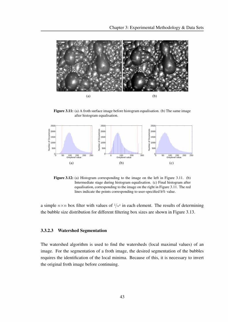
Chapter 3: Experimental Methodology & Data Sets
(a) (b)
Figure 3.11: (a) A froth surface image before histogram equalisation. (b) The same image
after histogram equalisation.
0 50 100 150 200 2500
500
1000
1500
2000
2500
Greylevel value
Num
ber
of O
ccur
ence
s
(a)
0 100 200 3000
500
1000
1500
2000
2500
Greylevel value
Num
ber
of O
ccur
ence
s
(b)
0 50 100 150 200 2500
500
1000
1500
2000
2500
Greylevel value
Num
ber
of O
ccur
ence
s
(c)
Figure 3.12: (a) Histogram corresponding to the image on the left in Figure 3.11. (b)
Intermediate stage during histogram equalisation. (c) Final histogram after
equalisation, corresponding to the image on the right in Figure 3.11. The red
lines indicate the points corresponding to user-specified h% value.
a simple n×n box filter with values of 1/n2 in each element. The results of determining
the bubble size distribution for different filtering box sizes are shown in Figure 3.13.
3.3.2.3 Watershed Segmentation
The watershed algorithm is used to find the watersheds (local maximal values) of an
image. For the segmentation of a froth image, the desired segmentation of the bubbles
requires the identification of the local minima. Because of this, it is necessary to invert
the original froth image before continuing.
43
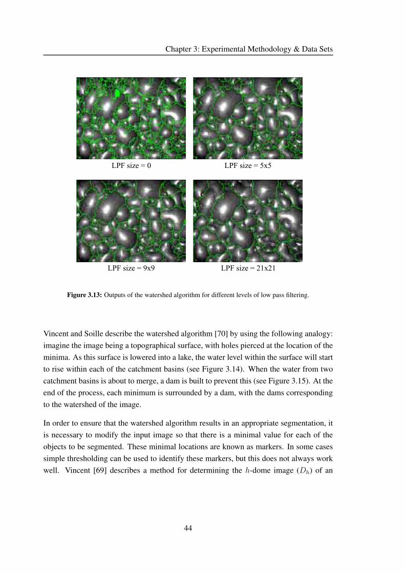
Chapter 3: Experimental Methodology & Data Sets
Figure 3.13: Outputs of the watershed algorithm for different levels of low pass filtering.
Vincent and Soille describe the watershed algorithm [70] by using the following analogy:
imagine the image being a topographical surface, with holes pierced at the location of the
minima. As this surface is lowered into a lake, the water level within the surface will start
to rise within each of the catchment basins (see Figure 3.14). When the water from two
catchment basins is about to merge, a dam is built to prevent this (see Figure 3.15). At the
end of the process, each minimum is surrounded by a dam, with the dams corresponding
to the watershed of the image.
In order to ensure that the watershed algorithm results in an appropriate segmentation, it
is necessary to modify the input image so that there is a minimal value for each of the
objects to be segmented. These minimal locations are known as markers. In some cases
simple thresholding can be used to identify these markers, but this does not always work
well. Vincent [69] describes a method for determining the h-dome image (Dh) of an
44

Chapter 3: Experimental Methodology & Data Sets
image (I), which can be applied for marker extraction:
Dh(I) = I − ρI(I − h), (3.1)
where ρI(J) is the greyscale reconstruction of I from J . This process is illustrated in
Figures 3.14 to 3.16.
A threshold is then applied to the h-dome image so as to generate a binary marker image,
M .
A homotopic transform is used to combine the marker image and the original image such
that the original image has minima where the markers are present and such that non-
catchment basins are filled up. This is achieved by calculating the modified image I ′
using a greyscale reconstruction [69]:
I ′ = ρ∗min(I+1,(m+1)M)((m + 1)M), (3.2)
where M is the binary marker image and m is the maximal value of pixels in I .
The watershed algorithm can be applied to the modified image, I ′, to determine the final
segmentation of bubbles. The output from the watershed segmentation for various low
pass filter values can be seen in Figure 3.13.
Once the segmentation has been calculated, it is possible to isolate each of the blobs in
the segmentation (a blob is a segmented region and ideally will correspond to a single
bubble). From the blobs it is possible to determine a bubble size distribution (in pixels2 or
in mm2 if calibrated). While the measurement presented here is typically referred to as the
bubble size, it is important to note that it is not in fact the true bubble size of the flotation
froth, as this in fact dependent on the 3D nature of the bubbles inside the froth. What is
actually being calculated is the surface film distribution of the flotation froth. Additional
measurements such as the circularity, ellipticity and Sauter mean bubble diameter (d32)
can easily be calculated. The Sauter mean diameter is the diameter of the sphere which
has the same volume/surface area ratio as the bubble being measured.
45

Chapter 3: Experimental Methodology & Data Sets
Figure 3.14: Minima, catchment basins and watersheds (Source: Vincent and Soille [70]).
Figure 3.15: Building dams as the water level rises (Source: Vincent and Soille [70]).
Figure 3.16: Determining h-domes from image I (Source: Vincent [69]).
46

Chapter 3: Experimental Methodology & Data Sets
3.3.3 Stability
For a detailed description of the stability algorithm, the reader is referred to Hatfield [25]
and Morar et al. [46]. A measure of the stability of the froth is calculated by examining
the difference between consecutive frames after image registration has taken place. The
image registration is achieved by taking a Fourier transform of both images. Typically
a subregion of 256×128 pixels is analysed (this being the largest area that is a power
of 2 that can be selected from a 320×240 pixel image). The Fourier transform of the
first image is multiplied by the complex conjugate of the Fourier transform of the second
image. The result is then transformed to the space domain, and normalised by the average
of the energy of the two images. The result of this operation is a matrix which has a peak
at the spatial offset between the two images. The height of the peak is also a measure
of how similar the two images are. Figures 3.17 to 3.20 show two images, their Fourier
transforms and the resulting correlation matrix which is used to register the two images.
The images are then registered, and the second frame is subtracted from the first. The
mean absolute difference between the registered frames can then be calculated and used
as a measure of the stability of the froth. An alternative calculation can be made by
determining the percentage of the image which has undergone a change greater than a
user-specified amount. This value is calculated by thresholding the absolute difference
image and calculating the percentage of pixels which have a value of one. Figure 3.21
shows the result of this calculation. The pixels which have been highlighted in red are
areas of the image which have undergone the user-specified amount of change since the
previous frame.
47

Chapter 3: Experimental Methodology & Data Sets
Figure 3.17: Two consecutive frames of video footage. Note the bubble that has burst.
Figure 3.18: Cropped areas of size 256×128 on which the Fourier transform can be easily
calculated.
Figure 3.19: Fourier transforms of corresponding images in Figure 3.18.
48

Chapter 3: Experimental Methodology & Data Sets
Figure 3.20: Space domain correlation peak.
Figure 3.21: Original image with red areas indicating the areas of change.
49

Chapter 3: Experimental Methodology & Data Sets
3.3.4 Velocity
Three velocity measures are discussed here. Typically only the first two (block matching
and bubble tracking) are used. In order to calculate a velocity measure, one needs to look
at a sequence of frames. Typical sequence lengths for SmartFroth vary between two and
five frames. The measurements are made for all consecutive pairs of frames and the mean
velocity measurement is used. All work in this thesis will be based on the block matching
velocity measurement unless otherwise specified.
3.3.4.1 Block Matching
The first frame is subdivided into a user-specified number of blocks. Cross correlation
is used to search within a window in the subsequent frame for the best match to each of
the individual blocks. In this way a motion vector field is generated. The mean values
of the motion vector field are used as the final velocity measure. For details on how the
block matching algorithm is performed efficiently, the reader is referred to the work of
Francis and de Jager [17]. A resultant motion vector field from using the block matching
algorithm is shown in Figure 3.22.
3.3.4.2 Bubble Tracking
As the watershed algorithm gives the output details of each individual bubble in the froth
image, it is possible to use this information to track bubbles over multiple frames to deter-
mine a velocity measure. The centroids of the bubbles are tracked over multiple frames,
with additional information such as bubble size being used to ensure that the same bubble
is matched in subsequent frames. Only bubbles which can be successfully tracked over
a given number of frames are used to calculate the final mean velocity measure. More
details can be found in Francis’ PhD Thesis [13]. A resultant motion vector field from
using the bubble tracking algorithm is shown in Figure 3.23.
3.3.4.3 Stability
As has already been mentioned, the froth stability measurement requires an image regis-
tration step. The output of this registration can be used as a coarse velocity measure. The
disadvantage of this velocity measure is that there is only one motion vector per frame.
50

Chapter 3: Experimental Methodology & Data Sets
Figure 3.22: Resulting motion vector field from the block matching velocity calculation.
Figure 3.23: Resulting motion vector field from the bubble matching velocity calculation.
51

Chapter 3: Experimental Methodology & Data Sets
3.4 Other Machine Vision Packages for Froth Flotation
This section gives a brief comparison of how commercially available machine vision sys-
tems for froth flotation make their measurements. Due to the commercial nature of these
products, it is often difficult to find accurate details on the algorithms they use. It is also
important to realise that the quality of measurement from any camera system is dependent
largely on two things, firstly the quality of the algorithms which make the measurements,
and secondly, the manner in which the installation has been set up (appropriate lighting,
zoom level, focus, etc.)
3.4.1 JK Frothcam
JK Frothcam was one of the original machine vision systems for analysing flotation froths.
It has not seen much development since its introduction in 1994.
Velocity measures are made using the pixel tracing technique [50]. Whilst this was ap-
propriate for the level of computing power available in the 1990s, this method sacrifices
accuracy for speed. It is in effect a block match using a single block. This means that it is
not robust against effects such as shearing and popping bubbles.
The texture spectrum is used to identify which class the froth is in by comparing against
the texture spectrums of user specified known classes [51].
The bubble size measurement is based on the MID_TU measurement from the texture
spectrum. A non-linear relationship has been shown to relate this measure to the mean
bubble size of certain flotation froths [30].
3.4.2 VisioFroth
VisioFroth was developed by Metso Minerals Cisa, with numerous installations found on
industrial flotation cells around the world.
VisioFroth uses a Fourier transform based method for calculating the froth velocity [58].
This method, is a fast way of calculating the disparity between two images. However, like
the pixel tracing algorithm, it can be adversely affected by popping and shearing bubbles.
52

Chapter 3: Experimental Methodology & Data Sets
The bubble size measurement used employs a watershed based approach [58]. Specific
details are hard to come by, but it has been acknowledged that the algorithm does not per-
form well when images with both large and tiny bubbles are present simultaneously [58].
It is not easy to determine how the VisioFroth stability parameter is calculated. However,
Runge et al. [58] mention a method that reports the change in bubble surface area, based
on the analysis of bubble size data from consecutive frames.
3.4.3 FrothMaster
Unlike other froth camera systems which send a video signal to a computer, the Out-
okumpu FrothMaster is a self contained device that outputs 4-20mA signals. It outputs,
froth velocity, stability and bubble size details. The available literature does not detail the
algorithms used by this camera system.
3.5 Texture Measures
The texture of a flotation froth image is related to the bubble size distribution of the flota-
tion froth. It is not always possible to accurately determine the bubble size distribution.
Under such circumstances it is best to use a texture measure to classify the flotation froth
instead. Examples of such instances will be dealt with later in Chapter 6.
Numerous texture measures have been proposed in literature, and many of them will be
outlined in the subsequent sections. There is no agreement on which texture method is
best suited to use on flotation froths. In fact, no comprehensive tests have been made
to determine which texture methods are best suited to flotation froths. The reason that
many texture measures exist is that different approaches are often suited for different
texture recognition problems. However, no texture measures have been designed with
flotation froths in mind. The temperature measurement analogy is appropriate here as
well. As there are many ways of determining temperature (alcohol thermometers, mercury
thermometers, thermocouples, solid-state integrated circuits, etc.), there are many ways
of measuring texture. However, unlike in the temperature case where an actual ground
53

Chapter 3: Experimental Methodology & Data Sets
truth exists from which we can determine how well our temperature measurement device
works for a given scenario, ground truth for texture is not well defined.
Texture measurements are typically tested by using a data set consisting of numerous
images of multiple textures. The textures are then divided into different classes, where
each class has members which have similar textures. Texture measures can then be used
to see how well they can discriminate between these classes. If they can discriminate
well, then they are good texture measures.
3.5.1 First Order Statistics
First order statistical methods are the simplest measures for the textural description of im-
ages. They describe the histogram of a greyscale image and contain no spatial information
about the image they describe. As a result, they are generally very poor at discriminating
between different textures. Furthermore, they are not invariant to illumination changes.
Figure 3.24 shows three different textures, all of which have the same histogram (Fig-
ure 3.25), and therefore the same first order statistics. This simple example shows that
they are a poor method for texture discrimination.
Figure 3.24: Three different textures with the same first order statistics.
54

Chapter 3: Experimental Methodology & Data Sets
0 50 100 150 200 2500
0.01
0.02
0.03
0.04
0.05
0.06
Greyscale Value
Num
ber
of O
ccur
ence
s
Figure 3.25: Histogram for textures in Figure 3.24.
Typical first order statistical features used for texture discrimination include [33]:
Mean:1
N
∑a,b
im(a, b) (3.3)
Variance:1
N − 1
∑a,b
(im(a, b) − mean)2 (3.4)
Standard Deviation:√
variance (3.5)
RMS Level:
√∑a,b im(a, b)2
N(3.6)
Integral:∑a,b
im(a, b) (3.7)
Skewness:1
N
∑a,b(im(a, b) − mean)3
standard deviation3 (3.8)
Kurtosis:1
N
∑a,b(im(a, b) − mean)4
standard deviation4 (3.9)
Entropy: −n−1∑i=0
pi log2(pi) (3.10)
Contrast:
n−1∑i=0
i2pi (3.11)
where
55

Chapter 3: Experimental Methodology & Data Sets
N is the number of pixels in the image
im(a, b) is the grey level value at point (a, b)
n is the total number of grey levels
pi = fi/N where fi is the frequency of occurrence of grey level i
3.5.2 Greyscale Co-occurrence Matrices
The use of greyscale co-occurrence matrices (GSCOMs) is based on Julesz’s conjec-ture, that the human eye uses similar second order statistics to discriminate between tex-
tures [20]. Greyscale co-occurrence matrixes (also referred to as grey level co-occurrence
matrices and grey-tone spatial-dependence matrices) describe the probability of neigh-
bouring pixels having certain grey level values. The greyscale co-occurrence matrix, Pij ,
is an n × n matrix which can be mathematically expressed as:
Pij =∑
a
∑b
u(a, b) (3.12)
where
u(a, b) =
{1 if s(a, b) = t(a − d1, b − d2)
0 otherwise(3.13)
and
s(a, b) =
{1 if im(a, b) = i
0 otherwise(3.14)
t(a, b) =
{1 if im(a, b) = j
0 otherwise(3.15)
(d1, d2) is the user-specified distance vector and im is the input image with n grey levels.
Haralick et al. suggested fourteen textural features that can be calculated from the
56

Chapter 3: Experimental Methodology & Data Sets
GSCOM. Features that are typically used in the literature include [22, 60, 54]:
Energy (Angular Second Moment):∑i,j
P 2ij (3.16)
Entropy: −∑i,j
Pij log Pij (3.17)
Contrast:∑i,j
|i − j|Pij (3.18)
Homogeneity:∑i,j
Pij
1 + |i − j| (3.19)
Correlation:∑i,j
(i − μx)(j − μy)Pij
σxσy
(3.20)
Inverse Difference Moment:∑i,ji�=j
Pij
|i − j| (3.21)
Maximum Probability: max(Pij) (3.22)
3.5.3 Fourier Ring/Wedge Filters
A combination of ring and wedge filters can be applied in the spatial frequency domain
in order to extract texture features [56, 63, 75]. The ring filters contain spatial frequency
information, while the wedge filters contain directional information. The power spectrum
of the Fourier transform is defined as:
E = |F (u, v)|2. (3.23)
The total power within the ring is computed:
fring =
∫ 2π
0
∫ r2
r1
|F (r, θ)|2 rdr dθ, (3.24)
where r1 and r2 define the ring filter (see Figure 3.26).
57
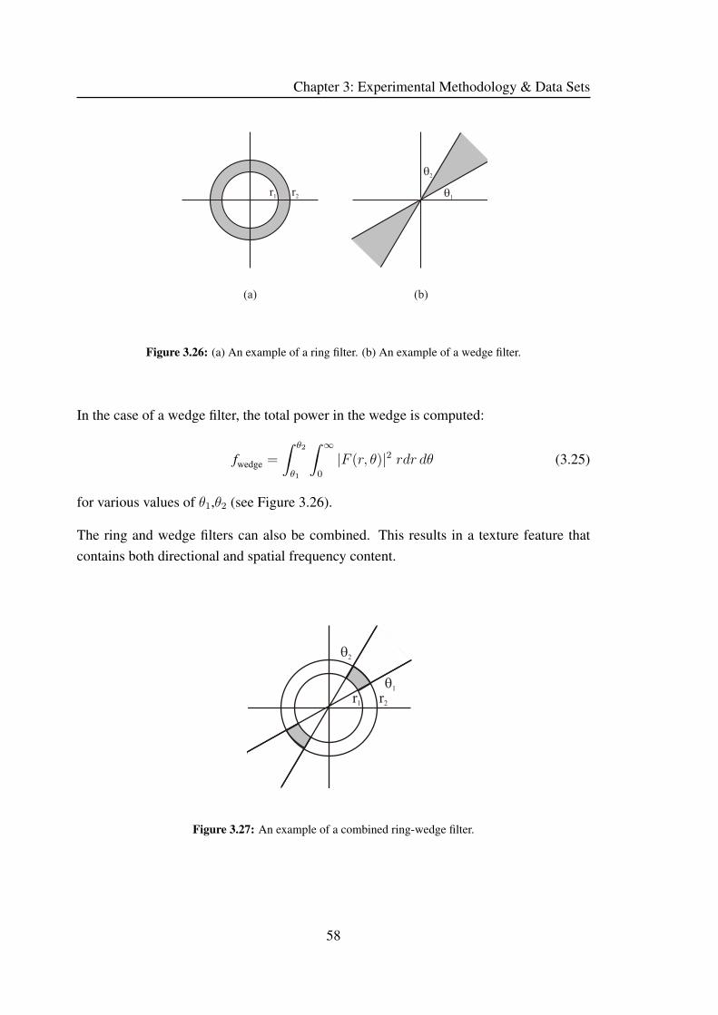
Chapter 3: Experimental Methodology & Data Sets
Figure 3.26: (a) An example of a ring filter. (b) An example of a wedge filter.
In the case of a wedge filter, the total power in the wedge is computed:
fwedge =
∫ θ2
θ1
∫ ∞
0
|F (r, θ)|2 rdr dθ (3.25)
for various values of θ1,θ2 (see Figure 3.26).
The ring and wedge filters can also be combined. This results in a texture feature that
contains both directional and spatial frequency content.
Figure 3.27: An example of a combined ring-wedge filter.
58

Chapter 3: Experimental Methodology & Data Sets
The total power in the combined ring/wedge region is computed:
fring,wedge =
∫ θ2
θ1
∫ r2
r1
|F (r, θ)|2 rdr dθ. (3.26)
3.5.4 Gabor Filter Bank
The Gabor filter bank technique for texture feature extraction is very similar to the
ring/wedge technique. The main difference is that the ring/wedge filter is replaced with
a Gabor filter (sinusoidally modulated Gaussian in the space domain). Figure 3.28 shows
the space and spatial frequency domain representation of a Gabor Filter.
(a) (b)
Figure 3.28: (a) Gabor filter in the space domain. (b) Contour plot of its spatial frequency
domain response.
The space domain response for the Gabor filter is given by the formula [40, 74]:
g(x, y) =(
12πσxσy
)exp
[− 1
2
(x′2σ2
x+ y′2
σ2y
)]exp
(2πix′
λ
)(3.27)
x′ = x cos φ − y sin φ (3.28)
y′ = x sin φ + y cos φ. (3.29)
59

Chapter 3: Experimental Methodology & Data Sets
While the spatial frequency domain response for the Gabor filter is given by the for-
mula [40, 74]:
G(u, v) = C exp[− 2π2
(σ2
x
(u′ − 1
λ
)2+ σ2
y(v′)2
)](3.30)
u′ = v cos φ − v sin φ (3.31)
v′ = u sin φ + v cos φ (3.32)
C = const. (3.33)
(a) (b)
Figure 3.29: (a) Gabor filter in the spatial domain. (b) The spatial frequency response of
the Gabor filter (after Wang et al. [74]).
Figure 3.29 shows the relationships between the various parameters in both the space and
spatial frequency domain.
Texture features are calculated by evaluating:
fgabor =
∫ ∞
0
∫ ∞
0
|G(u, v)F (u, v)|2 dudv (3.34)
G(u, v) is the spatial frequency domain Gabor filter response
F (u, v) is the Fourier transform of the input image
60

Chapter 3: Experimental Methodology & Data Sets
for a set of filters that have varying rotations (φ), wavelengths of the Gabor filter (λ) and
widths of the Gaussian kernel (σ2x and σ2
y), such that they majority of the spatial frequency
domain is covered by the set of filters.
3.5.5 Autoregressive 2D Linear Predictor Model
Simple linear predictors are used to predict the next value of a signal using previous
samples. The number of previous samples used is known as the order of the predictor.
For example, a 3rd order linear predictor, predicting sample number n, will have the
form:
s̃(n) =3∑
k=1
aks(n − k). (3.35)
The error between the actual value and the predicted value of sample number n is:
e(n) = s(n) − s̃(n). (3.36)
And so the total squared error over the whole signal is:
E =∑
n
e(n)2. (3.37)
61

Chapter 3: Experimental Methodology & Data Sets
For an optimal predictor, values of a1, ..., ap that minimise the total squared error, E, are
required. These values are determined by solving the set of linear equations:⎡⎢⎢⎢⎢⎢⎢⎣s3 s2 s1
s4 s3 s2
s5 s4 s3
......
...
sn−1 sn−2 sn−3
⎤⎥⎥⎥⎥⎥⎥⎦
⎡⎢⎢⎢⎢⎣a1
a2
...
ap
⎤⎥⎥⎥⎥⎦ =
⎡⎢⎢⎢⎢⎢⎢⎣s4
s5
s6
...
sn
⎤⎥⎥⎥⎥⎥⎥⎦ (3.38)
There are numerous methods that can be used to solve this set of linear equations, they
include:
• Covariance Method [38]
• Autoregressive Method [38]
• Cholesky Decomposition [55]
To be used as a textural feature for image classification, it is necessary to extend the linear
predictor to the two dimensional case, where s is the image on which the linear predictor
is based and s̃(n, m) is the prediction of the value of the image intensity at location (n, m)
and O is the order of the predictor:
s̃(n, m) =O∑
j=1
O∑k=1
ajks(n − j, m − k). (3.39)
The squared error is:
E2(n, m) =∑
n
∑m
(s(n, m) − s̃(n, m))2. (3.40)
The coefficients ajk can then be used as a texture feature describing the image on which
the linear predictor was created.
62

Chapter 3: Experimental Methodology & Data Sets
3.5.6 Laws’ Filter Masks
Kenneth Laws [34] suggests applying a set of convolution kernels, followed by a non-
linear windowing operation to calculate texture energy features from a greyscale image.
The set of convolution kernels is generated from the following set of one dimensional
convolution kernels:
L5 = [ 1 4 6 4 1 ]
E5 = [ -1 -2 0 2 1 ]
S5 = [ -1 0 2 0 -1 ]
W5 = [ -1 2 0 -2 1 ]
R5 = [ 1 -4 6 -4 1 ].
Laws also suggested kernels of length three and seven, but they will not be discussed
here. From the set of one dimensional kernels, it is possible to generate the following
twenty-five two dimensional kernels:
L5L5 E5L5 S5L5 W5L5 R5L5
L5E5 E5E5 S5E5 W5E5 R5E5
L5S5 E5S5 S5S5 W5S5 R5S5
L5W5 E5W5 S5W5 W5W5 R5W5
L5R5 E5R5 S5R5 W5R5 R5R5 .
All of these 2D kernels are zero mean, except for the L5L5 kernel, which is not used
to calculate a texture feature, but is only used for an optional normalisation step. Laws’
method [34] was developed to classify individual pixels according to their local texture.
In this work, entire images are classified as a single texture. Because of this, the algorithm
that follows explains how to determine a single texture feature for an image, rather than a
texture feature per pixel.
The input greyscale image is convolved with each of the 2D kernels, which results in a
set of twenty-five filtered images, Fk. For each of these filtered images, the total energy
is calculated:
Ek =∑i,j
|Fk(i, j)|. (3.41)
63

Chapter 3: Experimental Methodology & Data Sets
This results in a set of twenty-four texture energy images which can be used to distin-
guish between different textures (remember that the L5L5 kernel is not used for a texture
feature).
3.5.7 Texture Spectrum
The texture spectrum is simply a frequency plot of the texture units in a greyscale plot.
He and Wang [27] developed the texture unit as follows.
For a given pixel, its texture unit is calculated by comparing it to its eight neighbouring
pixels. The texture unit, TU , is the set of Ei (i=1,2,...,8) where:
Ei =
⎧⎪⎨⎪⎩0, if Vi < V0
1, if Vi = V0
2, if Vi > V0.
(3.42)
Figure 3.30: Labelling of neighbourhood pixels.
Figure 3.30 shows the ordering of pixels used for the calculation in equation 3.42. The
texture unit number is then calculated using the following formula [27]:
NTU =8∑
i=1
Ei 3i−1. (3.43)
Figure 3.31 shows an example of how the texture unit number is determined from an input
pixel and its neighbourhood. In this manner, each pixel in an image can be labelled with
64

Chapter 3: Experimental Methodology & Data Sets
Figure 3.31: Example of determining the texture unit number from a neighbourhood of
pixels (after He and Wang [27]).
a specific texture unit number, NTU . The texture spectrum, S(i), is simply the frequency
distribution of these texture units. Not only do He and Wang suggest using the sum of
absolute differences as a distance measure between two texture spectra [27], but they also
suggest that certain texture features can be calculated from texture spectra [28]:
Black-White Symmetry =
[1 −
3279∑i=0
|S(i) − S(3281 + i)|6560∑i=0
S(i)
]× 100 (3.44)
Geometric Symmetry =
[1 − 1
4
4∑j=1
6560∑i=0
|Sj(i) − Sj+4(i)
2 ×6560∑i=0
Sj(i)
]× 100 (3.45)
Degree of Direction =
[1 − 1
6
3∑m=1
4∑n=m+1
6560∑i=0
|Sm(i) − Sn(i)|
2 ×6560∑i=0
Sm(i)
]× 100. (3.46)
65

Chapter 3: Experimental Methodology & Data Sets
They then go on to suggest a number of oriented texture features: the micro-horizontal
structure (MHS), the micro-vertical structure (MVS) and two micro-diagonal structures
(MDS1, MDS2):
MHS =6560∑i=0
S(i) × HM(i) (3.47)
MVS =6560∑i=0
S(i) × VM(i) (3.48)
MDS1 =6560∑i=0
S(i) × DM1(i) (3.49)
MDS2 =6560∑i=0
S(i) × DM2(i), (3.50)
where:
HM(i) = P (E1, E2, E3) × P (E5, E6, E7) (3.51)
VM(i) = P (E1, E8, E7) × P (E3, E4, E5) (3.52)
DM1(i) = P (E1, E2, E8) × P (E4, E5, E6) (3.53)
DM2(i) = P (E2, E3, E4) × P (E6, E7, E8) (3.54)
and P (Ea, Eb, Ec) represents the number of elements in {Ea, Eb, Ec} which have the
same value for texture unit i.
Finally, they propose the central symmetry feature:
Central Symmetry =6560∑i=0
S(i) × K(i)2 (3.55)
where K(i) is the number of pairs having the same values in the elements: (E1, E5),
(E2, E6),(E3, E7) and (E4, E8) for texture unit i.
66
Chapter 3: Experimental Methodology & Data Sets
3.5.8 Wavelets
The wavelet decomposition of an image is computed by applying a series of high and
low pass filters and subsequent sub-sampling. This process is shown graphically in Fig-
ure 3.32.
The input image (L0) is decomposed into a low resolution low pass filtered image, L1
and a set of detail images {D(h)1 , D
(v)1 , D
(d)1 }. This process is then repeated for the image
L1 for a user-specified number of times. The end result of this process is a multiscale
representation of the image L0 of depth d: {Li, D(h)i , D
(v)i , D
(d)i }i=1..d. Figure 3.33 shows
the wavelet decomposition for an image.
Texture features are typically created by taking the mean and standard deviation of the
energy in each of the sub-bands of the wavelet decomposition [3, 64, 65, 40]. These
features are referred to as the wavelet energy signatures.
Mallat [39] found experimentally that the histograms of the sub-bands of the wavelet
decomposition of an image can be modelled according to the family of exponentials:
h(u) = K e−(|u|α
)β
, (3.56)
where K is a normalisation constant. Van de Wouwer suggests that this model can be used
for texture characterisation by using the wavelet histogram signature {α, β} as a texture
feature for each of the sub-bands of the wavelet decomposition of an image. Further
details of the calculation of α and β can be found in [64].
Finally, Van de Wouwer suggests that using second order statistics instead of first order
statistics to describe each of the sub-bands of the wavelet decomposition should provide
better texture features than the wavelet histogram signatures. He suggests using wavelet
co-occurrence signatures which are obtained by calculating the co-occurrence matrix and
eight suggested features calculated from the co-occurrence matrix. These calculations are
done in the same manner as those specified in Section 3.5.2, except that the processing is
done on the sub-bands of the wavelet decomposition instead of on the original image.
67

Chapter 3: Experimental Methodology & Data Sets
2 1
1 2
1 2
1 2
1 2
2 1
Low Pass(rows)
Low Pass(cols)
Low Pass(cols)
High Pass(rows)
High Pass(cols)
High Pass(cols)
2 1 : Downsample columns1 2 : Downsample rows
Li
Li+1
Di+1
Di+1
Di+1
(h)
(v)
(d)
Figure 3.32: Flow diagram of a single step of decomposition using the discrete wavelet
transform.
Figure 3.33: Example of the wavelet decomposition of an image to depth 2.
68

Chapter 3: Experimental Methodology & Data Sets
3.6 Classification Methods
Classification algorithms “learn” characteristic features of different data sets, and can
then classify new data as belonging to one of the initial data sets. For example, a classifier
could be trained to determine whether a froth belongs to the large, fast moving bubbles
set or the small, slow moving bubbles set based on the froth’s bubble size and velocity
measurements. As with most engineering situations, tradeoffs exist. For classification
algorithms the tradeoffs typically involve performance, time to learn, time to classify new
data and complexity of the algorithm. The algorithms described are not overly compli-
cated, but provide a good basis on which decisions about the quality of measurements can
be made.
Classifiers typically undergo a training and a testing stage to determine how effective
they are at classifying input data. To achieve this, labelled data is required. Labelled
data has the associated known category for each of the input vectors. This data set is
then subdivided into testing and training data sets. The allocation of data to these sets is
typically done in a random manner. The classifier then undergoes training on the training
data set; this involves adjusting model parameters to the training data set. The classifiers
performance is then determined by classifying the data in the test data set and calculating
how many of the data points were correctly labelled.
Numerous classification methods have been developed over the years; they are however
beyond the scope of this thesis and will not be discussed. A few classifiers which are used
in this thesis are presented below.
3.6.1 Geometric Separability Index
Testing and training classifiers is a time consuming task. Thornton [62] developed a
separability index which can be quickly calculated for a data set and which gives a good
indication of how successful a classifier based on this data will be. Another advantage is
that there is no need to split the data into training and testing data sets. Thornton defines
69

Chapter 3: Experimental Methodology & Data Sets
the geometric separability index (GSI) as:
GSI(f) =
n∑i=1
[f(xi) + f(x′i) + 1] mod 2
n, (3.57)
where f is a binary target function, x is the data set, x′i is the nearest neighbour of xi and
n is the total number of data points.
This can easily be extended to the case where there are multiple classes of data:
GSI(f) =
n∑i=1
c(xi, x′i)
n(3.58)
where
c(a, b) =
{0, if f(a) �= f(b)
1, if f(a) = f(b)(3.59)
with f being a target function (no longer limited to the binary case).
The GSI calculates the fraction of the data set which have nearest neighbours of the same
class. As such, a value of one indicates a high degree of separability as all data points have
nearest neighbours of the same class. A value of 0.5 corresponds to two random data sets
with the same centre point. This number decreases as the number of classes increases,
and will have the value of 1/n for n random data sets of the same size with the same centre
point. Figure 3.34 shows a few possible GSI values for a variety of different data sets.
3.6.2 KNN Classification
K nearest neighbour (KNN) classifiers are the general case of the nearest neighbour clas-
sifier. A suitably large data set of labelled data is required for the nearest neighbour
classifier. When a new datum is to be classified, the distance between it and all samples
in the labelled data set are computed. The datum is classified as belonging to the class of
the closest point in the labelled data set. Figure 3.35 shows a graphical illustration, where
the new datum (black dot) is classified as having the same class (class 1) as its nearest
neighbour (black circle).
70

Chapter 3: Experimental Methodology & Data Sets
0 5 10 150
5
10
15Geometric Separability Index: 0.00000
Class 1Class 2
0 5 10 150
5
10
15Geometric Separability Index: 0.43000
Class 1Class 2
0 5 10 150
5
10
15Geometric Separability Index: 0.95000
Class 1Class 2
0 5 10 150
5
10
15Geometric Separability Index: 0.25333
Class 1Class 2Class 3
Figure 3.34: A few examples of different data sets and their geometric separability in-
dices.
The k nearest neighbour algorithm is similar, but a vote is held between the k nearest
neighbours to determine which class a new datum belongs to. An example of a k nearest
neighbour (k = 5) classifier is shown in Figure 3.36 where two of the nearest neighbours
belong to class 1 (red) and three belong to class 2 (blue). The resultant class allocation
will be class 2 as it is in the majority.
The main advantage of k nearest neighbour classifiers is their ease of implementation.
Their disadvantages include the storing of large labelled data sets for the classification of
new data and the processing time required to classify a new data point because of the large
number of distance calculations that need to be made. Further processing can remedy this
situation. For example a kd-tree data structure may be used for efficient determination of
the nearest neighbours.
71

Chapter 3: Experimental Methodology & Data Sets
−3 −2 −1 0 1 2 3 4
−2
−1
0
1
2
3
4
Class 1Class 2New Data Point To ClassifyNearest Neighbour
Figure 3.35: Classifying a new data point using a nearest neighbour classifier.
−6 −4 −2 0 2 4 6 8
−2
0
2
4
6
8
Class 1Class 2New Data Point To ClassifyNearest Neighbours
Figure 3.36: Classifying a new data point using a k nearest neighbour classifier.
72

Chapter 3: Experimental Methodology & Data Sets
3.6.3 Gaussian Mixture Models
Gaussian mixture models (GMM) are a probability density representation of a data set.
A multi-dimensional data set can be represented as a summation (mixture) of Gaussian
kernels and is illustrated in Figures 3.37 to 3.39. The method of fitting the Gaussian
kernels to the data is outlined below.
The user specifies the number of Gaussian kernels to be used. Initial estimates of the
centres, covariances and weights of the kernels are required. Typical initialisation uses
the k-means algorithm to generate starting points for the centres of the kernels.
After the initialisation, an iterative process of optimising the kernels’ centres and covari-
ances is performed. This process is known as the expectation maximisation algorithm.
The aim of the expectation maximisation process is to optimise the likelihood that the
data points were generated from the Gaussian mixture model. The algorithm iterates
between the following two steps:
1. Expectation Step. The data points are evaluated to determine the likelihood that
they belong to each of the Gaussian kernels being used to describe the data set. Each
point has an associated probability of being associated with each of the kernels.
2. Maximisation Step. The parameters of the kernels are re-estimated using a weight-
ing of the data points that reflects the likelihood of the kernel for explaining that data
point.
These steps are repeated until convergence occurs or a pre-specified number iterations
has been performed. The expectation maximisation algorithm does not guarantee that a
global optimum solution will be found, so good initial starting values are required.
Figure 3.40 shows the iterative process of the expectation maximisation algorithm to fit
two Gaussian mixtures to a data set. The colours of the data points (changing from blue
through purple to red) indicate the relative probability of belonging to the two Gaussian
kernels.
Classification can be achieved by fitting a GMM to each class of labelled data. When a
new datum is to be classified, its probability of being generated by each of the GMMs can
be quickly evaluated, with the class allocation being made to the class associated with the
most probable GMM.
73

Chapter 3: Experimental Methodology & Data Sets
The advantages of GMMs is that once they have been trained, classification of new data
points is extremely fast. Data storage for the trained classifier is also minimal as only a
few details about the Gaussian mixture models are required.
74

Chapter 3: Experimental Methodology & Data Sets
0 5 10 15 20 250
5
10
15
20
25
Figure 3.37: An example data set.
0 5 10 15 20 250
5
10
15
20
25
Figure 3.38: A Gaussian mixture model representation of the data set in Figure 3.37, using
two centres for each class.
05
1015
2025
0
5
10
15
20
250
0.05
0.1
0.15
0.2
Figure 3.39: A 3D Gaussian mixture model representation of the data set in Figure 3.37.
75

Chapter 3: Experimental Methodology & Data Sets
(a) (b) (c)
(d) (e) (f)
(g) (h) (i)
Figure 3.40: Iterating through a Gaussian mixture model fitting process (after Nabney and
Bishop [47].
76

Chapter 3: Experimental Methodology & Data Sets
3.7 Distribution Distance Measures
The formulae for various distance measures to compute the dissimilarity between distri-
butions are given below. These measurements are used in Chapter 4 to learn frequently
occurring bubble size distributions.
For a more detailed description of these measures, the reader is referred to Rubner et
al. [57]. These authors distinguish between marginal and complete histograms because
their work is based on the comparison of various image related features. In the work pre-
sented in this thesis this distinction is not required as only one dimensional distributions
are compared, so the differences between marginal and complete histograms is not made.
For the equations shown in the sections below, D(X, Y ) is the dissimilarity between
distributions X and Y . The quantity f(i, X) is entry number i of the distribution of
X and F (i, X) is entry number i of the cumulative distribution of X .
3.7.1 Kolmogorov-Smirnov
The Kolmogorov-Smirnov distance measure is defined as the maximum discrepancy be-
tween two cumulative size distributions. It is calculated by the formula:
D(X, Y ) = maxi
|F (i, X) − F (i, Y )|. (3.60)
3.7.2 Chi Square
The chi square statistic (χ2) is given by the formula:
D(X, Y ) =∑
i
(f(i, X) − f(i,X)+f(i,Y )
2
)2
f(i,X)+f(i,Y )2
. (3.61)
77

Chapter 3: Experimental Methodology & Data Sets
3.7.3 Cramer / von Mises Distance
The Cramer / von Mises Distance (CvM) distance measure is defined as the squared Eu-
clidean distance between the distributions:
D(X, Y ) =∑
i
(F (i, X) − F (i, Y )
)2. (3.62)
3.7.4 Jeffrey-divergence
The Jeffrey-divergence (JD) is defined by:
D(X, Y ) =∑
i
(f(i, X) log
f(i, X)f(i,X)+f(i,Y )
2
+ f(i, Y ) logf(i, Y )
f(i,X)+f(i,Y )2
). (3.63)
3.7.5 Minkowski Distance
The general form of the Minkowski distance measure is:
D(X, Y ) =( ∑
i
|f(i, X) − f(i, Y )|p) 1
p. (3.64)
Special cases of the Minkowski distance measure are frequently used:
1. Cityblock (p = 1)
2. Euclidean (p = 2)
3. Maximal (p = inf).
3.8 Other Techniques
Two additional methods, namely principal component analysis and unsupervised classifi-
cation, are presented in the next to sections. Both of these methods are used in Chapter 4.
78

Chapter 3: Experimental Methodology & Data Sets
3.8.1 Principal Component Analysis
Principal component analysis (PCA) is often used to reduce the dimensionality of high
dimensional data so that is easier to work with. This is achieved by projecting the data
onto orthogonal axes which represent the largest variations in the data.
Principal component analysis is performed as follows. First the data are normalised to
have zero mean and unit standard deviation. Next the eigenvectors and eigenvalues for
the data are calculated. The eigenvector corresponding to the highest eigenvalue is the first
principal component of the data set, and explains most of the variation seen in the data
set. The eigenvector associated with the second highest eigenvalue is the second principal
component and so on. The data can easily be rotated around the eigenvectors, and the
lower order principal components can be removed so as to reduce the dimensionality of
the data, whilst preserving as much of the variance as possible. Figure 3.41 shows the
reduction of two dimensional data to one dimensional data using principal component
analysis.
3.8.2 Unsupervised Classification
Unsupervised classification techniques are useful when labelled data sets do not exist.
Unsupervised classifiers attempt to automatically label the data by determining the clus-
ters inherent to the data. Many different unsupervised clustering algorithms exist. They
are beyond the scope of this work, and only the hierarchical unsupervised clustering al-
gorithm used in this thesis is discussed.
The hierarchical clustering algorithm goes through the following steps:
1. All data points are considered clusters, and an associated inter-distance matrix Dij
is calculated. The Euclidean distance between the data points is typically used, but
any distance measure appropriate to the task may be used.
2. Search through the inter-distance matrix to determine the clusters i and j corre-
sponding to the smallest element Dij(i �= j). Merge clusters i and j to form a new
cluster.
3. Calculate the dissimilarity between the new cluster and the remaining clusters and
then generate a new inter-distance matrix. When using the nearest neighbour
method, the distance between the new cluster, {i, j}, and another cluster, k, is
79

Chapter 3: Experimental Methodology & Data Sets
−15 −10 −5 0 5 10 15−15
−10
−5
0
5
10
15
Data Points1st Principal Component2nd Principal Component
(a)
−15 −10 −5 0 5 10 15−15
−10
−5
0
5
10
15
Data Points1st Principal Component2nd Principal Component
(b)
−15 −10 −5 0 5 10 1−1
−0.8
−0.6
−0.4
−0.2
0
0.2
0.4
0.6
0.8
1
(c)
Figure 3.41: (a) Data with principal components. (b) Data rotated around principal com-
ponent axes. (c) Data reduced to one dimension by removing 2nd principal
component.
80

Chapter 3: Experimental Methodology & Data Sets
given by min{Dik, Djk}. When using the furthest neighbour method, the distance
between the new cluster, {i, j}, and another cluster, k, is given by max{Dik, Djk}.
4. Repeat steps 2 and 3 until all clusters have been merged.
The result is what is known as a dendrogram, which shows the relative similarities of the
different clusters. Figure 3.42 shows an example of a dendrogram and the data from which
it was generated. The dendrogram can be “cut” into a user-specified number of branches
(clusters) to determine the final class allocations of the clustering algorithm. For example,
if the dendrogram in Figure 3.42 was cut so as to have three clusters, the resulting clusters
would be: {A, G, F,H, B}, {C, D} and {E}.
81

Chapter 3: Experimental Methodology & Data Sets
0 2 4 6 8 100
1
2
3
4
5
6
7
8
9
10
A
B
C
D
E
F
G
H
(a)
A G F H B C D E
(b)
Figure 3.42: (a) Data set of eight points. (b) Dendrogram created from data in (a) using
nearest neighbour method.
82

Chapter 3: Experimental Methodology & Data Sets
3.9 Introduction to the Data Sets & Froth Classification
The next sections detail the various data sets that will be used in this thesis. The first
data set consists of flotation froth images from a variety of industrial installations around
the world. The next four data sets come from industrial sites that process a variety of
metals (copper, molybdenum and platinum group metals). These data sets also include
metallurgical data that was sampled at the same time as the collection of video footage.
3.10 Froth Image Data Set
The froth image data set was created by the author by extracting frames from sequences
of video footage corresponding from a variety of different sources.
The froth classes in the froth image data set come from a variety of sources, including
copper, zinc, phosphate, molybdenum and platinum concentrators. This data set is de-
signed to be a good overview of all the types of froths that can occur (with the notable
exception of coal froths). The idea behind this selection is that if good performance can
be achieved on this data set, then it is likely that the measure will be suitable for the clas-
sification of most flotation froths. Figure 3.43 shows some example images from the froth
image data set. The full set of images in the data set can be found in Appendix B.
Eighteen froth classes were identified by selecting visually different (bubble size and
texture differences) flotation froths. The set of images within each class are consistently
visually similar, while images from the different classes are visually dissimilar. The froth
image data set consists of 18 different classes. The number of example images in each
class is variable, but is typically 1000 with a minimum of 300 example images per froth
type. The data set consists of a total of 16793 images, each with a resolution of 320×240
pixels.
83

Chapter 3: Experimental Methodology & Data Sets
Figure 3.43: Some sample images from the froth image data set. Each row is a different
texture class.
84

Chapter 3: Experimental Methodology & Data Sets
3.11 Discussion on Industrial Data Sets
Before introducing the specific details of the individual industrial data sets that are used
in this thesis, this section discusses various relevant aspects of the data sets, including the
sampling procedure, the reason for using four industrial data sets, and the identification
of froth classes.
3.11.1 Physical Sampling
The physical sampling process involved the collection of feed, concentrate and tailings
samples. At the time of sampling (which occurred once the plant was under steady state
conditions), the feed, concentrate and tailings samples were collected simultaneously. At
the same time, video footage of the flotation froth was collected. The concentrate grade
was a cumulative sample typically collected over a five minute period. In the cases where
the sampled flotation cell was the first cell in the bank, the feed sample was collected
from the bank feed stream with a sample cutter. In the case where the sampled cell was
preceded by other flotation cells, the feed was approximated by the pulp sample of the
preceding cell, collected using an in-pulp sampler. The cell tailings were approximated
by the flotation pulp of the cell being sampled, collected by means of another in-pulp
sampler at a location near the tailings valve.
Due to the duration of the sampling (typically five minutes) and the proximity of the
camera system to the location of the collection of the concentrate grade sample, it is
expected that the samples are a representative “snapshot” of the instantaneous flotation
cell conditions and are not likely to be adversely affected by the cell residence time.
3.11.2 Experimental Test Design
The goal of the test work in the industrial data sets was primarily to determine whether re-
lationships exist between the machine vision froth surface descriptors and the concentrate
grade of the flotation cell. Specific step tests have not been made, as such approaches of-
ten have results which are only valid when the other variables (which were kept constant
for the test) remain inside a narrow range.
85

Chapter 3: Experimental Methodology & Data Sets
It is important to note that the tests were conducted under what can be considered as
typical operating conditions. This is important because it can be easier to perform test
work under extreme conditions, and find relationships which explain these conditions.
However, such relationships are often not sensitive enough to be useful in the typical
operating conditions under which personnel try to keep the flotation cells.
3.11.3 Number of Data Sets
In this work, four different industrial data sets have been used. The reasons for using four
different industrial data sets as opposed to one larger data set are outlined below. The
main advantage of having one larger data set is the availability of a large number of data
points. By having a large number of data points it is much easier to determine if any
observed relationships are real.
Despite this limitation when using smaller data sets, provided the appropriate statistical
methods are employed, one can still determine whether the observed relationships are real
(statistically significant) or not. The disadvantage is that it is more likely that one will not
be statistically confident in observed relationships.
The first advantage of using multiple data sets is the diversity of the flotation froths that are
covered. It is one of this thesis’s objectives to show that a unified approach for modelling
concentrate grade exists that can be applied to most flotation froth systems (objective
number five, see Section 2.9). It would not be appropriate to extrapolate findings based
on one data set to cover multiple flotation froth systems.
In order to have a unified approach, it is necessary to have an appropriate set of froth
surface descriptors which can handle a wide range of froths. Had only one data set been
used, the developments to froth surface descriptor measurements in Chapter 4 would not
have been made. This would have resulted in a set of results that were only applicable to
one flotation froth system.
86

Chapter 3: Experimental Methodology & Data Sets
3.11.4 Froth Classes
The introduction of froth classes instead of using continuous measurements is an impor-
tant aspect of this work which needs to be explained. The identification of froth classes is
the process whereby the video samples in the data sets are manually identified into visu-
ally similar sets. This process is similar to the way an experienced flotation cell operator
would differentiate between different froth states, before making changes to the appropri-
ate setpoints as necessary. In this work, the froth classes have been identified by looking
primarily at the bubble size distribution of the froth videos. The number of froth classes
identified is not fixed, but is rather dependent on the range of visible conditions that were
apparent during the sample campaign. However, experience on the data sets used in this
thesis has shown that this number is typically less than five for a flotation cell running
under normal operating conditions. It is likely to increase under other scenarios such as
the testing of different reagents.
One of the elements of the work presented in this thesis, is the need to reduce high di-
mensionality data so that it is easier to work with. For example, Section 4.2 deals with
the problem of reducing a bubble size distribution to a single value descriptor. The diffi-
culty of dealing with high dimensional bubble size data is further complicated when one
deals with flotation froths which exhibit dynamic bubble size distributions. The use of
classification and feature extraction methods for the reduction of high dimensional data is
common in the field of pattern recognition [5].
Dealing with high dimensional data is difficult for two reasons. Firstly, one suffers from
the “curse of dimensionality” which means that there is an exponential increase in the
amount of data required to appropriately populate the sample space with each increasing
dimension [5]. This essentially means that it is not possible to determine the relationships
between high dimensional and other data without over-fitting the data. Secondly, it is
often difficult to work with high dimensional data because it is difficult to visualise and
may not have any physical meaning. This is particularly true for flotation cell operators
who prefer to work with measurements which have direct meaning [66].
This potential disadvantage of using single value descriptors is highlighted in Section 4.2.
An approach is needed that reduces the complexity of using high dimensional data such as
complete bubble size distributions or the high dimensional texture features when texture
87

Chapter 3: Experimental Methodology & Data Sets
measures are used. The solution to this is to have an intermediate state which contains as
much information as possible, but is easier to work with. Classifying the flotation froth
samples into visually similar classes can achieve this intermediate state. Furthermore,
the various froth classes are easily understandable by plant personnel, unlike using other
dimensionality reduction techniques such as principal component analysis, to which it is
difficult to attach any physical meaning.
The introduction of froth classes does reduce the amount of information pertaining to
the current state of the flotation froth. However it is a necessary step towards the un-
derstanding of the relationships between the metallurgical performance and the flotation
froth measurements. Once these initial relationships have been identified, it will justify
the use of the more complex methods required to relate the high dimensional data with
metallurgical performance. As long as the reduction associated with the introduction of
froth classes is acknowledged, and checks are performed to determine if the use of froth
classes is acceptable, the use of classification as a data reduction technique is appropriate.
3.11.5 Identification of Froth Classes
The froth classes identified in the subsequent sections were manually identified by clas-
sifying the video sequence samples into “visually similar” classes. Before this process
was performed, the filename associated with each of the video sequences was randomised
to ensure that no prior knowledge pertaining to the conditions of the sampling biased the
classification. Each froth class contains video segments which are visually similar to each
other. Generally this means that the flotation froths will have a similar bubble size distri-
bution. In the case of flotation froths with dynamic bubble size distributions, the dynamic
nature of the froth is also taken into account.
The number of froth classes identified is entirely dependent on the data set being classi-
fied. It is just coincidence that the molybdenum, platinum data and copper 2004 data set
were classified into four froth classes.
88

Chapter 3: Experimental Methodology & Data Sets
The classification into froth classes is done in much the same way that experienced flota-
tion cell operators make adjustments to the process variables based on their observations
of the state (class) of the froth. Other researchers, including Bartolacci et al. [4], Nguyen
and Thornton [51] and Aldrich et al. [2] have used this method of identifying froth classes.
The froth classes identified have been independently corroborated by experienced person-
nel so as to ensure that they represent ground truth as far as possible. The results observed
in Chapters 5 to 7 show the validity of the froth classes as they have different metallur-
gical relationships associated with them. This would not have been the case for random
froth class allocation.
The reason for using froth classes rather than a set of continuous variables based on either
bubble size or texture measurement is because this approach still remains a difficult chal-
lenge, requiring substantial amounts of data to ensure statistical confidence in observed
results. Once the relationships between froth classes and metallurgical performance have
been established, it can be used as a foundation for further research into using continuous
measurements.
3.12 Platinum Data Set
The platinum data set was collected at the Anglo Platinum Amandelbult UG2 Concentra-
tor from 21 to 23 January 2003.
3.12.1 Experimental Setup
The test work was conducted on the first rougher cell at the Amandelbult UG2 platinum
concentrator. Due to the limited time duration of the test work, it was necessary to ar-
tificially induce different froth states by making changes to the air, level and reagent
setpoints. The reason for this was to induce visually different froth classes in the flotation
cell.
When the flotation cell was operating under steady state conditions, feed and concentrate
metallurgical samples and video samples were collected so that the relationship between
89

Chapter 3: Experimental Methodology & Data Sets
the froth texture and the metallurgical performance of the cell could be determined. The
video footage was recorded to video tape so that in-depth analysis could be run offline at
a later stage. The metallurgical samples were sent for assay analysis to determine their
elemental composition. Twenty sets of feed, concentrate and video footage samples were
collected.
3.12.2 Assays
The concentrate and feed samples were analysed for:
1. Copper (Cu)
2. Platinum Group Minerals (PGM)
3. Nickel (Ni)
4. Iron (Fe)
5. Sulfur (S)
6. Chromite (Cr2O4).
The assay results for individual samples are presented in Appendix A.
3.12.3 Froth Classes
After the sampling campaign was completed, the video was divided into clips of footage
of two minutes duration that correspond to the times at which metallurgical samples were
taken. This resulted in 26 video clips each corresponding to a set of metallurgical samples
taken. These clips were then classified into visually similar froth classes without using
any of the information about what conditions the cells were in at the time the footage was
taken. Four froth classes were identified; sample images of each of these are shown in
Figure 3.44. Video footage of the different froth classes is shown in Appendix B.
90

Chapter 3: Experimental Methodology & Data Sets
(a) Foamy froth. A mixture of bubbles and foam.
(b) Mainly foam, with rapidly popping bubbles.
(c) Mainly bubbles, with a few small areas of foam.
(d) Very stable froth. Only bubbles.
Figure 3.44: Sample images of the four froth classes identified on the platinum first
rougher.
91

Chapter 3: Experimental Methodology & Data Sets
3.13 Molybdenum Data Set
This section describes the experimental setup for the molybdenum data set. The test
work was performed on the third rougher of the molybdenum circuit at the Kennecott
Utah Copper Concentrator from 3rd February to 10th February 2006. During this time
fifty-four sets of samples were collected. The molybdenum circuit at Kennecott has the
concentrate stream from the copper circuit as its feed. The molybdenum is floated and the
copper depressed. The result is that the concentrate stream is rich in molybdenum and the
tailings are rich in copper.
3.13.1 Camera Installation
It was necessary to install a camera on the cell to be monitored. Since the test work
was only performed over one week, a temporary solution was used. This consisted of
mounting a commercial camcorder and halogen light above the cell. Figure 3.45 shows
the camera and light above the cell being monitored.
3.13.2 Process Adjustments
One of the goals of the test work was to determine a variety of froth classes under normal
operating conditions. In order to achieve this, it was necessary to make adjustments to
some of the process set-points. The ranges of adjustments made is shown in Table 3.1.
Table 3.1: Range of process adjustments for test work on rougher 3 of the molybdenum
circuit.
Parameter Low Value High Value
Froth Depth 4.5" 11"
pH 10.9 11.7
Initially, changes were planned for the nitrogen addition to the cell, but it was unfeasible
as it would require making adjustments to the nitrogen addition to the other cells in the
92

Chapter 3: Experimental Methodology & Data Sets
Figure 3.45: SmartFroth camera and lighting system installed on rougher 3 of the molyb-
denum circuit.
bank as well. Appendix C contains the process parameters for the duration of the test
work.
3.13.3 Samples
Eighteen sets of steady state conditions were sampled. This totalled 54 feed, 54 bulk
concentrate, 54 tails, and 18 top-of-froth samples. Five minutes of video footage of the
cell was taken to coincide with the physical sampling of the cell, this totalled 54 video
clips of rougher 3 of the molybdenum circuit.
Samples were taken in sets of three when the process was deemed to have reached a
steady state. Despite being at steady state, it was expected that there would be slight
93

Chapter 3: Experimental Methodology & Data Sets
differences in the velocities of the froth at the time of sampling, due to uncontrollable
plant disturbances. The sets of samples were typically taken fifteen minutes apart. Shorter
periods were used when the froth velocity was high so as not to flood the concentrate
sumps.
At each sampling time, the following samples were taken:
1. Feed Sample
2. Tails Sample
3. Bulk Concentrate Sample
4. Top-of-Froth Concentrate Sample.
Due to the small amount of concentrate accumulated when taking a top-of-froth sample,
one cumulative sample was taken for each steady state condition, unlike the other samples
for which three samples were taken for each steady state condition.
3.13.4 Assays
All of the samples collected were assayed for the following by the Kennecott laboratories:
1. Copper (Cu)
2. Iron (Fe)
3. Magnesium Oxide (MgO)
4. Molybdenum Disulfide (MoS2).
Additional measurements made included:
1. Percentage solids
2. Concentrate mass flow rate.
Selected feed and top-of-froth samples were also selected for mineralogical analysis us-
ing the mineral liberation analyser (MLA). The assay results for individual samples are
presented in Appendix A.
94

Chapter 3: Experimental Methodology & Data Sets
3.13.5 Froth Classes
During the sampling campaign four distinct froth types were identified. Example images
of the froth types are shown in Figure 3.46. The full set of video segments from this data
set can be found in Appendix B.
95

Chapter 3: Experimental Methodology & Data Sets
(a) Stable froth. Well formed loaded bubbles.
(b) Pulpy froth. Visible pulpy areas between bubbles.
(c) Sliming Froth. Large areas of pulp visible.
(d) See-through froth. Small transparent bubbles.
Figure 3.46: Sample images of the four froth classes identified on the molybdenum circuit
third rougher.
96

Chapter 3: Experimental Methodology & Data Sets
3.14 Copper 2004 Data Set
The copper 2004 data set was collected on the 1st rougher cell on row four at the Ken-
necott Utah Copper Concentrator from 21 April to 6 May 2004. During this time 30 sets
of samples were collected.
3.14.1 Camera Installation
A permanent installation of the camera, LED ring for illumination and hood was made for
this test work. The output of the camera was sent to the control room via coaxial cable,
where it was recorded onto SVHS video tapes for later processing.
3.14.2 Process Adjustments
The goal of the test work was to identify a set of visually different froth classes so that
links between the classes and the metallurgical performance of the cell could be investi-
gated. In order to achieve this in a short period of time, adjustments were made to the
process parameters. They are shown in Table 3.2.
Table 3.2: Range of process adjustments for test work on rougher 1, row four of the copper
circuit.
Parameter Low Value High Value
Froth Depth 7.2" 9.9"
pH 8.9 10.5
Frother 0.0007 lb/ton 0.0602 lb/ton
Collector 0.01 lb/ton 0.04 lb/ton
3.14.3 Samples
Thirty sets of steady state conditions were sampled. This totalled 30 feed, 30 bulk concen-
trate and 30 tails samples. One minute of video footage of the cell was taken to coincide
97

Chapter 3: Experimental Methodology & Data Sets
with the physical sampling of the cell, this totalled 30 video clips of rougher 1, row 4 on
the copper circuit.
Samples were taken in sets of three when the process was deemed to have reached a
steady state. Despite being at steady state, it was expected that there would be slight
differences in the velocities of the froth at the time of sampling, due to uncontrollable
plant disturbances. The sets of samples were typically taken ten minutes apart.
At each sampling time, the following samples were taken:
1. Feed Sample
2. Tails Sample
3. Bulk Concentrate Sample.
3.14.4 Assays
All of the samples collected were assayed for the following by the Kennecott laboratories:
1. Copper (Cu)
2. Iron (Fe)
3. Molybdenum (Mo).
Additional measurements made included:
1. Percentage solids.
The assay results for individual samples are presented in Appendix A.
3.14.5 Froth Classes
During the campaign, four froth classes were identified. Sample images of the froth
classes are shown in Figure 3.47. It is important to realise that the froth classes from the
Kennecott copper circuit are particularly dynamic, and as such, a small set of still images
is not sufficient to characterise the data set. The reader is referred to the video clips in the
electronic Appendix B for a better understanding of the differences between these froth
classes.
98
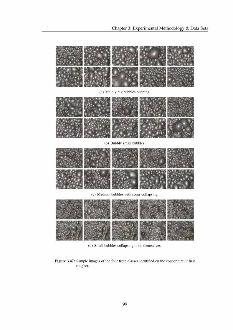
Chapter 3: Experimental Methodology & Data Sets
(a) Mainly big bubbles popping.
(b) Bubbly small bubbles.
(c) Medium bubbles with some collapsing.
(d) Small bubbles collapsing in on themselves.
Figure 3.47: Sample images of the four froth classes identified on the copper circuit first
rougher.
99

Chapter 3: Experimental Methodology & Data Sets
3.15 Copper 2006 Data Set
The 2006 copper data set was collected at the Kennecott Utah Copper Concentrator from
19 to 31 January 2006. All of the test work was conducted on the first rougher cell on row
four.
3.15.1 Camera Installation
The existing SmartFroth camera system on cell 1, row 4 was experiencing problems with
its lighting. The lighting system was swapped with a replacement system which worked
well. See Figure 3.48 for the camera and hood mounted on cell 1.
3.15.2 Process Adjustments
One of the goals of the test work was to gather data for a variety of froth classes which are
likely to occur under normal plant operating conditions. In order to achieve this, it was
necessary to make adjustments to some of the process set-points at various times. Details
of these values are given in Table 3.3.
Table 3.3: Process Adjustments made for the 2006 copper data set.
Parameter Low Value High Value
Froth Depth 7.3" 10.0"
Frother Dosage 0.015 lbs/ton 0.03 lbs/ton
Ideally, this test work campaign would have been conducted without making any changes
to the process parameters. Plant operators would be allowed to make the appropriate
changes as they saw fit, and froth video footage would have been collected as different
froth classes arose. Unfortunately, this approach could not be used due to time constraints.
This meant it was necessary to make adjustments to process parameters to ensure that a
range of froth classes were identified.
The froth depth parameter was primarily adjusted in order to obtain similar looking froths
with different froth velocities. This helped to populate the sample space for a variety
100

Chapter 3: Experimental Methodology & Data Sets
Figure 3.48: SmartFroth camera and hood system installed on cell 1, row 4 of the Ken-
necott copper circuit.
of different velocities for each froth class. The frother dosage was adjusted in order to
change the visual appearance of the froth.
Unlike sampling campaigns which are designed using the factorial method and aim to
sample at a variety of pre-specified values for each of the process parameters being ad-
justed, the goal of this sampling campaign was to generate a set of visually different froth
classes over a range of froth velocities. The input parameters which caused these froth
classes were of secondary interest. They will however be an important part of future
studies to determine how it is best to move between the different froth classes.
All other process parameters were left to be adjusted by the plant operators as per usual
101

Chapter 3: Experimental Methodology & Data Sets
operating procedure. Appendix C contains the process parameters for the duration of the
test work.
3.15.3 Sampling
Samples were taken in sets of three when the process was deemed to have reached a
steady state. Despite being at steady state, it was expected that there would be slight
differences in the velocities of the froth at the time of sampling, due to uncontrollable
plant disturbances. The sets of samples were typically taken fifteen minutes apart.
At each sampling time, the following samples were taken:
1. Feed Sample
2. Tails Sample
3. Bulk Concentrate Sample
4. Top-of-Froth Concentrate Sample.
Due to the small amount of concentrate accumulated when taking a top-of-froth sample,
one cumulate sample was taken for each steady state condition, unlike the other samples
for which three samples were taken for each steady state condition.
3.15.4 Analyses
Over the period 19 Jan 2006 to 31 Jan 2006, 35 sets of steady state conditions were
sampled. This totalled 105 feed, 105 bulk concentrate, 105 tails, and 35 top-of-froth
samples. Five minutes of video footage of the cell was taken to coincide with the physical
sampling of the cell, this totalled 105 video clips of cell 1, row 4 of the copper circuit.
The video footage can be viewed in Appendix B.
3.15.4.1 Assays
All of the samples collected were assayed for the following by the Kennecott laboratories:
102

Chapter 3: Experimental Methodology & Data Sets
1. Copper (Cu)
2. Iron (Fe)
3. Magnesium Oxide (MgO)
4. Molybdenum Disulfide (MoS2).
Additional measurements made included:
1. Percentage solids
2. Concentrate mass flow rate.
The assay results for individual samples are presented in Appendix A. Selected feed and
top-of-froth samples were also selected for mineralogical analysis using the MLA.
3.15.4.2 Video Analyses
Each of the 105 video clips was analysed using both SmartFroth and MATLAB to deter-
mine the following parameters:
1. Bubble size distribution for each frame of video
2. Froth velocity for consecutive frames of video
3. Froth texture for each frame of video.
103

Chapter 3: Experimental Methodology & Data Sets
104

Chapter 4
Measurement Advances
This chapter presents novel techniques for the improved measurement of froth surface
descriptors using machine vision technology. In so doing, it addresses the first three
objectives of this thesis.
Firstly, objective number one is addressed by showing that the current state of the art
bubble size measurements are not able to accurately segment froth images that contain
both large and tiny bubbles in the same image. An improved algorithm is presented and
shown to be able to achieve good segmentation under such conditions.
Next, objective number two is addressed. First, by introducing the concept of dynamic
bubble size distributions, and then by showing that the traditionally used single value
bubble size descriptors such as mean, p80, etc. can be inappropriate measures to use
for such flotation froths. Finally, various methods of characterising flotation froths with
dynamic bubble size distributions are presented and discussed.
Thirdly, objective number three of this thesis is addressed. Selected commonly used tex-
ture measures are tested on a suitably large data set of flotation froth images to determine
which texture measurement(s) are best suited for the analysis and classification of flota-
tion froth images.
105

Chapter 4: Measurement Advances
4.1 Improving the Watershed Segmentation Using Tex-ture Measures
4.1.1 Limitations of the Watershed Algorithm
Some flotation froths have fairly consistent bubble size distributions. Some examples of
such flotation froths can be seen in Figure 4.1. The watershed algorithm provides good
bubble segmentation in such cases. However, when both large and tiny bubbles appear in
flotation froths at the same time, the watershed algorithm performs poorly. Examples of
such flotation froths can be seen in Figure 4.2.
It is well known that the watershed algorithm performs poorly when both large and tiny
bubbles are present in an image simultaneously. Botha [7] suggested using the marker
bubble area ratio to determine areas of tiny bubbles. He also found that the texture mea-
sure of small number emphasis could be used to determine areas of tiny bubbles. However,
this method was deemed unfeasible due to excessive computation time and the sensitivity
to various parameters. Runge et al. [58] also acknowledge that the watershed algorithm
in VisioFroth is not able to successfully delineate the bubbles when both large and tiny
bubbles are present in a flotation froth image.
Wang et al. [71] have developed an algorithm to segment bubbles using valley-edge de-
tection and tracing techniques. They show that by classifying images into small, medium
or large bubbles, better segmentation can be achieved. However, they do not deal with the
case in which the flotation froth image has both large and tiny bubbles.
Figure 4.3 shows the typical results from using a watershed segmentation on an image
with both large and tiny bubbles. By adjusting the parameters of the watershed algorithm
(mainly the amount of low-pass filtering) it is possible to either under-segment the image
(and correctly identify the large bubbles) or over-segment the image (and correctly iden-
tify the tiny bubbles). It is not possible to correctly segment both the large and the tiny
bubbles simultaneously.
106

Chapter 4: Measurement Advances
(a) (b)
Figure 4.1: (a) Four flotation froth images for which the traditional watershed algorithm
segmentation works well and (b) their corresponding segmentations after run-
ning the watershed algorithm.
107

Chapter 4: Measurement Advances
(a) (b)
Figure 4.2: (a) Four flotation froth images for which the traditional watershed algorithm
segmentation works poorly and (b) their corresponding segmentations after
running the watershed algorithm.
108

Chapter 4: Measurement Advances
(a) (b)
Figure 4.3: (a) Over-segmentation of a froth image (note that all of the tiny bubbles are
correctly segmented, but the large bubbles are over-segmented). (b) Under-
segmentation of a froth image (note that all of the large bubbles are correctly
segmented, but the tiny bubbles are under-segmented).
4.1.2 Overview of proposed improvement
It is proposed that the segmentation of flotation froth images with both large and tiny
bubbles can be achieved by performing multiple passes of the watershed algorithm to
localised areas of the image, such that the areas with large bubbles are processed with
different parameters to the areas with tiny bubbles. This is achieved by initially identifying
the large bubbles correctly and under-segmenting the tiny bubbles. A texture measure can
then be applied to classify the blobs as either large bubbles or collections of tiny bubbles.
The original image can then be modified so that when the watershed algorithm is run
again, the tiny bubbles are correctly identified.
4.1.3 Classification of Tiny Bubbles
The first step to improve the watershed algorithm is to be able to identify which bubbles
have been correctly segmented and which bubbles have been under-segmented. Visual
109

Chapter 4: Measurement Advances
inspection of the results of the under-segmentation of froth images suggested that a tex-
ture measure would be appropriate to perform this classification. A data set of correctly
segmented large bubbles and under-segmented collections of tiny bubbles was generated
by hand from watershed segmented images from class 2 and 13 of the froth image data
set (see Appendix B). These data sets were chosen because they both contained clear
examples of both large and tiny bubbles in the same image. Figure 4.4 shows some exam-
ples from each class. The data set consisted of 108 examples of single bubbles and 107
examples of under-segmented collections of tiny bubbles.
As discussed in Chapter 3, there are numerous potential texture measures to use. Tests
were performed to determine how well the greyscale co-occurrence based texture mea-
sures and Laws’ 3×3 kernel based texture measures were at distinguishing between sin-
gle bubbles and collections of tiny bubbles. These texture measures were chosen because
of their ability to process small images of irregular shape. The texture spectrum was not
evaluated as it was expected that the small images would result in sparse texture spectrums
being generated.
The geometric separability index was used to determine which subsets of features were
best able to distinguish between the two data sets. The results are shown in Ta-
bles 4.1 to 4.4.
For Laws’ texture measures, at least four features are required to achieve reasonable clas-
sification. For the GSCOM measurements, 100% correct classification was possible for
all feature sets that included the contrast measure. It is clear that the contrast measure is
the best suited of the texture measures tested for the discrimination between single large
bubbles and collections of tiny bubbles. It is important to note that the data set on which
the testing was performed is somewhat artificial in that the data was chosen by hand to be
good examples of either single bubbles or collections of tiny bubbles. As such, ambiguous
cases were not selected and it is likely that 100% correct classification will not be always
achieved.
110

Chapter 4: Measurement Advances
(a)
(b)
Figure 4.4: (a) A subset of the data set of well segmented bubbles. (b) A subset of the
data set of under-segmented collections of tiny bubbles.
111

Chapter 4: Measurement Advances
Table 4.1: Separability indices for the data set using 3×3 Laws filters.
Features UsedSeparability
Index
E3E3 E3S3 S3S3 L3S3 L3L3 0.9581
E3E3 E3S3 S3L3 L3L3 0.9535
E3E3 S3E3 S3S3 S3L3 L3L3 0.9535
E3E3 S3S3 L3S3 L3L3 0.9535
E3E3 E3S3 S3E3 S3S3 S3L3 L3L3 0.9488
Table 4.2: Legend for features based on GSCOM for Tables 4.3 and 4.4.
Feature Number Feature Name
1 Maximum Probability
2 Energy
3 Contrast
4 Homogeneity
5 Entropy
Table 4.3: Separability indices for the data sets using GSCOM features.
Features Used Separability Index
1 2 3 4 5 1.000
1 2 3 4 1.000
1 2 3 5 1.000
1 2 3 1.000
1 3 4 5 1.000
1 3 4 1.000
1 3 5 1.000
1 3 1.000
2 3 4 5 1.000
2 3 5 1.000
2 3 1.000
3 4 5 1.000
3 5 1.000
3 1.000
1 2 4 5 0.995
Table 4.4: Separability indices using single GSCOM features.
Feature Separability Index
3 1.000
4 0.986
5 0.684
1 0.544
2 0.540
112
Chapter 4: Measurement Advances
4.1.4 Contrast
An examination of the GSCOM and the contrast feature show why this feature performs
particularly well in its ability to discriminate between single bubbles and collections of
tiny bubbles. Figure 4.5 shows an example of the GSCOM for both a single bubble and a
collection of tiny bubbles.
It is evident from Figure 4.5 that there is a distinct difference between the two GSCOMs
for the single bubble and the collection of tiny bubbles. The GSCOM for the single bubble
has high values along the diagonal. This is because neighbouring pixels in an image of
a single bubble tend to have similar values. The GSCOM for the image of a collection
of tiny bubbles on the other hand has a closer to uniform distribution. This is because
neighbouring pixels often have dissimilar intensities. It is because of these differences in
the GSCOM that the contrast feature:
Contrast:∑i,j
(i − j)2Pij (4.1)
can successfully discriminate between single bubbles and collections of tiny bubbles. This
is evident from the (i − j)2 term which emphasises terms far away from the diagonal.
Similarly, the homogeneity feature also performs well. It has the term |i − j| in the
denominator which emphasises terms along the diagonal of the GSCOM.
4.1.5 Modifying the Watershed
It is not simple to merge two watershed segmentations that have been created using dif-
ferent parameters. This is because there is no guarantee that the segmentation lines will
overlap one another. The method for applying and merging the results from multiple
passes of watershed segmentations is now discussed.
4.1.5.1 First Pass
The traditional watershed algorithm is applied to a flotation froth image, using a large
value for low-pass filtering to ensure that the large bubbles in the image are correctly seg-
113

Chapter 4: Measurement Advances
(a)
(b)
Figure 4.5: (a) Typical surface plot of a GSCOM for a single bubble and the image from
which it was generated. (b) Typical surface plot of a GSCOM for a collection
of tiny bubbles and the image from which it was generated.
114

Chapter 4: Measurement Advances
mented and that the tiny bubbles are under-segmented. Each blob in the image is then
classified according to its contrast value (determined from the greyscale co-occurrence
matrix). An example of an input image, the under-segmented watershed output, and clas-
sification of blobs is shown in Figures 4.6, 4.7 and 4.8 respectively.
4.1.5.2 Input Image Modification
From the classification results it is possible to generate a mask which identifies areas of
single bubbles, collections of tiny bubbles and bubble boundaries. An example of such
a mask is show in Figure 4.9. The original input image is then filtered using a low-
pass filter once more, but this time, less low pass filtering is used, to ensure the accurate
segmentation of the small bubbles. Figure 4.10 shows the result of applying the mask
to the low-pass filtered image. The result is achieved by modifying the low-pass filtered
input image such that the areas corresponding to blobs which have been identified as
single bubbles by the classification step have maximal values. The pixels which border
these single bubbles are given minimal values. The areas of the image corresponding to
collections of tiny bubbles in the classification step remain unchanged.
4.1.5.3 Second Pass
The watershed algorithm is then performed on the modified input image. Because of the
modification to the input image, the boundaries of the large bubbles are guaranteed to
be correctly identified. The tiny bubbles will also be correctly identified as they have
not been processed with too much low-pass filtering. Figure 4.11 shows the resulting
segmentation after the second watershed pass has been applied. A flow diagram of the
entire process is shown in Figure 4.12.
4.1.6 Discussion
The algorithm discussed here performs well at segmenting individual bubbles when the
flotation froth image has both large and tiny bubbles. A two-pass algorithm has been
discussed, but it is possible to extend this to an n-pass algorithm. Experience has shown,
however, that segmentation performance does not improve if more than three passes are
115

Chapter 4: Measurement Advances
Figure 4.6: Input image for segmentation.
Figure 4.7: 1st pass of watershed algorithm resulting in under-segmentation.
Figure 4.8: Results of classification according to contrast. Blue indicates single bubbles
and yellow collections of tiny bubbles.
116

Chapter 4: Measurement Advances
Figure 4.9: Classification mask generated from Figure 4.8.
Figure 4.10: Input image, after it has been low pass filtered and had the mask applied to
it.
Figure 4.11: Final watershed segmentation.
117

Chapter 4: Measurement Advances
Figure 4.12: Flow sheet of the two-pass watershed algorithm.
118

Chapter 4: Measurement Advances
used (when a image size of 320×240 pixels is used). This is most likely due to the
increasing number of parameters that need to be optimised to achieve good segmentation.
It is expected that if a larger images size is used (1024×768 pixels for example), then
the relative size of the large and tiny bubbles in the image will be different to those in
a smaller (320×240 pixels) image. Under such circumstances it is likely that more than
three passes could provide better segmentation results.
Determining the optimal parameters for a segmentation is non-trivial. The determination
of the parameter settings is best achieved using a visual approach in which the first stage
of low pass filtering is adjusted so that the large bubbles are correctly identified. When
this has been achieved, the threshold of the contrast based classifier should be adjusted
such that only single bubbles are correctly identified. Finally, the second pass low-pass
filtering should be adjusted such that an accurate segmentation is achieved for the tiny
bubbles as well.
In order to set up the parameters for an industrial flotation cell which contains both large
and tiny bubbles, it is necessary to capture video footage of the flotation cell under a
variety of conditions (all large bubbles, all tiny bubbles, and intermediate states) so that
optimal parameters can be determined that can correctly segment individual bubbles for
all of these cases.
119
Chapter 4: Measurement Advances
4.2 Reducing BSD Data For Classification
This section examines the reduction of bubble size distribution information for froth clas-
sification. To overcome the high dimensionality of bubble size distribution data, it is
typically reduced to either a mean [53, 12, 30, 32] , median (p50) or p80 value. Alterna-
tively, the data is reduced to a set of classes such as {small, medium, large} [61]. These
reductions are not always appropriate, and can result in the loss of most of the informa-
tion contained in a bubble size distribution. Whether or not such reduction of the data is
appropriate or not is generally not considered.
4.2.1 Dynamic Bubble Size Distributions
Certain froth types exhibit what has been termed “dynamic bubble size distributions”.
These dynamic BSDs occur when a flotation froth under steady state conditions has sub-
stantially different bubble size distributions over a short period of time. Not all flotation
froths exhibit this kind of behaviour, nor is it dependent on the mineral being mined. An
example of two frames of footage taken within one second of each other from a froth
which has a dynamic BSD is shown in Figure 4.13. The figure shows that two images
taken within one second of each other can have very different bubble size distributions.
The reader is referred to the copper 2006 video footage in Appendix B for a better under-
standing of the nature of flotation froths with dynamic bubble size distributions.
The correct sampling of these dynamic froths is extremely important. A single sample is
clearly insufficient to characterise such a dynamic steady state froth as the resulting BSD
measurement could have a huge range of values depending on the exact timing of when
the sample was taken. With this in mind, a set of tests was devised to determine how
effective individual bubble size measurements are at characterising such froths.
The tests were each devised with the goal of capturing certain aspects of the nature of
froths with dynamic bubble size distribution. The ideas behind the different methods
are presented here, with detailed descriptions of their implementation in the following
sections.
120

Chapter 4: Measurement Advances
A B
100
101
102
103
104
0
20
40
60
80
100
Bubble Size [pixels2]
Per
cent
age
Pas
sing
Cumulative Bubble Size Distribution
AB
Figure 4.13: An example of a froth with a dynamic BSD. The BSDs are taken from two
frames of video which are within 1 second of each other.
The single value descriptors (mean, median, p80) technique attempts to overcome the
dynamic nature of froths by sampling for a long period of time. By increasing the number
of samples, improved performance is expected as the resulting measurement will be based
on a more representative sample than measurements made from shorter sequence lengths.
The BSD search algorithm attempts to improve on the single value descriptor method
by actively searching for an optimal decision point (unlike the singular value descriptor
method which relies on a fixed decision point). Like the single value descriptor method,
better results are expected when longer, more representative samples are taken.
By not reducing the BSD to a single value, the aggregate BSD algorithm aims to retain the
information which is lost when single value descriptors are used. Once again, increased
sample length is expected to improve results in a more representative sample of the froth.
Because of the averaging nature of the aggregate BSD algorithm, neither the different
states of the froth, nor the transitions between the states are accounted for.
121

Chapter 4: Measurement Advances
The reduced dimensionality aggregate BSD algorithm is based on the aggregate BSD al-
gorithm. Once again, the additional information present in the bubble size distribution
is maintained, but in this case principal component analysis is used to reduce the dimen-
sionality.
The frequently occurring BSD algorithm attempts to characterise dynamic froths accord-
ing to the percentage of time that they are in different states. These states correspond to
different bubble size distributions. In so doing the dynamic nature of the froth is better
accounted for. Like the other methods, frequently occurring BSDs does not account for
the sequencing of transitions between the different states.
Observation and experimentation on dynamic flotation froths indicates that the state tran-
sitions are not easily captured by simple models and appear to be largely random. Because
of this, no algorithm has yet been developed which accounts for the state transitions.
There is room for further research in this area.
4.2.2 Testing Methodology
Two data sets were used for this set of tests, the platinum data set and the 2004 copper
data set. The data sets were chosen for the following reasons. The platinum data set is a
good example of a froth which does not exhibit a dynamic BSD. The copper 2004 data set
was chosen because it is a good example of a data set which does exhibit a dynamic BSD.
For both data sets, labelled froth classes already exist which can be used for determining
performance values.
The objectives of the tests were to:
1. determine whether reducing bubble size distributions to a single value, such as
mean, median or p80, is appropriate or not.
2. determine what video clip duration (number of frames) needs to be analysed in
order to overcome the problems associated with sampling dynamic BSDs.
3. determine which algorithms are best suited to classifying the state of the froth, using
bubble size information alone.
122
Chapter 4: Measurement Advances
In this work, tests are performed to determine whether certain measurements provide the
user with valuable information. These tests are similar to sensitivity tests / signal-to-noise
ratio tests. The test is constructed as follows:
Firstly, two distinctly different conditions that the user would like the measurement being
tested to be able to discriminate between, are hand picked. An analogous example would
be trying to discriminate between an apple (condition one) or an orange (condition two)
using some measurement.
Next, selected measurements are taken from a large data set containing examples of both
conditions. In the analogous example, consider measuring the diameter of fruit as a mea-
surement. Consider a data set of diameters for apples and oranges. The data set can be
analysed to determine how successfully a new fruit will be classified (as either an apple
or orange), based solely on its diameter. If it is found that apples and oranges have similar
diameters, then one can conclude that the measurement of a fruit’s diameter is not suitable
for determining if it is an apple or an orange.
This work proceeds in a similar manner, except that the measurement being analysed
will be related to the bubble size of a froth (for example, mean, median or p80). The
conditions will not be fruit, but rather images of froths at steady state, with different
bubble size distributions. If the mean bubble size (for example) is not able to distinguish
between two froth states, then the conclusion is that measuring the mean bubble size is
inappropriate, and a different measure of bubble size must be used.
4.2.3 Single value descriptors
The method of testing for single value descriptors will be discussed for the mean bubble
size calculation. It is straightforward to use the method for other calculations such as
median and p80. The mean bubble size calculation simply needs to be replaced with the
desired calculation.
The method discussed here does not provide any novel measurement of bubble size for
dynamic flotation froths. Instead, a methodology is proposed with which it is possible to
determine the suitability of using single value descriptors for the classification of dynamic
flotation froths.
123

Chapter 4: Measurement Advances
A single random sample of consecutive frames is taken from one of the video segments
in the data set. Figure 4.14 shows how multiple three frame samples can be drawn from a
video segment. Note how the starting frame for each of the samples is random, so they are
not in consecutive order. From these frames, the bubble size distribution can be calculated
using the advanced watershed algorithm (Section 4.1). The mean bubble size can then be
calculated for the sample.
This process of sampling and calculating the mean bubble size for a sample is repeated
many times. Since there are multiple samples, there are multiple values for the mean bub-
ble size. It is therefore possible to plot the distribution of mean bubble size measurements
for a froth class. Figure 4.15 shows an examples of such a distribution of mean bubble
size measurements.
The process of calculating the mean bubble size distribution for a class is done for two
froth classes from a data set. The desired result is that the mean bubble size distributions
from the two froth classes will be centred at different points and not be overlapping. Gen-
erally, it is unlikely that the two distributions will not have some degree of overlap. By
scanning along the mean bubble size axis, it possible to determine the point which will
maximise the classification performance (optimal decision boundary) of the two froth
classes by discriminating based on their mean bubble size value. Figure 4.16 shows an
example of two well separated mean bubble size distributions for two froth classes. Fig-
ure 4.17 shows an example of two poorly separated mean bubble size distributions for two
froth classes.
Once the optimal decision boundary for two froth classes has been determined, it can be
used for the classification of new samples. The mean bubble size is calculated for the new
sample and is then classified as belonging to one of the two classes depending on which
side of the decision boundary the mean value lies on.
For each class, all sequences of frames of lengths {1, 2, 3, 4, 5, 7, 10, 14, 19, 26, 37,
51, 71, 98, 136, 189, 262, 364, 504, 700} were extracted subject to there not being an
overlap of frames of more than one third the length of the sequence. In order to determine
how well the mean bubble size measurement performs at distinguishing between froth
classes, all the samples were taken for a given froth class and randomly allocated to either
a training or testing data set. For each combination of froth classes, the optimal decision
boundary was determined on the training data set. The testing data set was then used
124

Chapter 4: Measurement Advances
Time
Sample 1
Sample 3
Sample4
Sample2
Figure 4.14: An example of drawing numerous 3-frame samples from a video sequence.
0 50 100 1500
0.02
0.04
0.06
0.08
0.1
0.12
0.14
0.16
0.18
0.2
Mean Bubble Size [pixels2]
Fre
quen
cy
Figure 4.15: Mean bubble size distribution for sequences of four frames for froth class 2
from the platinum data set.
125

Chapter 4: Measurement Advances
0 50 100 150 200 250 300 350 400 450 5000
0.02
0.04
0.06
0.08
0.1
0.12
0.14
0.16
0.18
0.2
Mean Bubble Size [pixels2]
Fre
quen
cyClass B (Platinum Data Set)Class D (Platinum Data Set)Optimal Decision Boundary
Figure 4.16: Mean bubble size distributions for sequences of four frames for two well
separated froth classes.
0 50 100 150 200 250 300 350 400 450 5000
0.02
0.04
0.06
0.08
0.1
0.12
0.14
0.16
0.18
0.2
Mean Bubble Size [pixels2]
Fre
quen
cy
Class C (Platinum Data Set)Class D (Platinum Data Set)Optimal Decision Boundary
Figure 4.17: Mean bubble size distributions for sequences of four frames for two poorly
separated froth classes.
126

Chapter 4: Measurement Advances
to determine the performance of the mean bubble size measurement. This process was
repeated for both the platinum and the 2004 copper set for a variety of frame sequence
lengths.
4.2.4 BSD search
The BSD search method is similar to the reduction of the bubble size distribution to a
mean, p50 or p80 value. The difference is that the BSD is not reduced to a predefined
percentile, but rather a search is made to determine the optimal percentile to discriminate
between two classes based on a single measurement.
Once again, samples are taken from the data set. Cumulative bubble size distributions are
calculated for each of the samples. A scan is then performed for each value on the bubble
size axis. For each value, the distribution of percentage passing the current bubble size
values is plotted and once again, an optimal decision boundary can be determined. See
Figure 4.18 for an illustrative example of how this is achieved for two froth classes.
1 10 52100 1000 100000
10
20
30
40
50
60
70
80
90
100
Training DataCumulative Bubble Size Distribution
Bubble Size [pixels2]
Per
cent
age
Pas
sing
0 20 40 60 80 1000
10
20
30
40
50
60
70
80
90
100
Per
cent
age
Pas
sing
Number of Occurrences
Histogram of Percentage Passingfor Bubble Size: 52
Class A (Platinum)Class D (Platinum)Optimal Decision Boundary
Figure 4.18: BSD search for determining the optimal percentage passing value for two
froth classes.
127

Chapter 4: Measurement Advances
In this manner, an optimal decision boundary and optimal percentage passing a given
bubble size value can be determined. These values are calculated for a training data set.
After this, performance values can be determined for a test data set for differing sequence
lengths in both the platinum and 2004 copper data set.
4.2.5 Aggregate BSDs
The aggregate BSD method tries to account for the time aspect of the dynamic bubble
size distribution by merging the bubble size data from a sequence of frames. The bubble
size information is calculated for a sequence of frames of video. The bubble size mea-
surements are then combined to generate a single cumulative bubble size distribution for
the video sequence. This single cumulative BSD for the whole video sequence is referred
to as the aggregate BSD.
For each froth class, samples can be taken from the training data set. For each of these
samples, a single aggregate BSD is calculated. The result is a set of aggregate BSDs
associated with each froth class.
Next, it is necessary to determine a set of characteristic aggregate BSDs. These charac-
teristic aggregate BSDs are determined by using a hierarchical unsupervised clustering
algorithm. It is necessary to have an appropriate distance measure to compare the dis-
similarity of the aggregate BSDs. Various distance measures were tested: Kolmogorov-
Smirnov, chi square, Cramer / von Mises, Jeffery divergence and the Minkowski metric.
Results from tests to determine the best distance measure for bubble size distributions
showed no significant differences in performance. As a result, the Kolmogorov- Smirnov
distance measure was used because it is an intuitive distance measure for BSDs and is
easy to implement.
Figure 4.19 shows the results from using hierarchical unsupervised classification to de-
termine the characteristic aggregate BSDs for two froth classes (class 1 and class 2). The
left hand side of Figure 4.19 shows the entire set of aggregate BSDs for each of the froth
classes. The right hand side of Figure 4.19 shows the resulting sets of nine characteristic
BSDs for each of the froth classes. Characteristic BSDs A to I were determined from
class 1, and BSDs K to R were determined from class 2. The number of frequently occur-
128
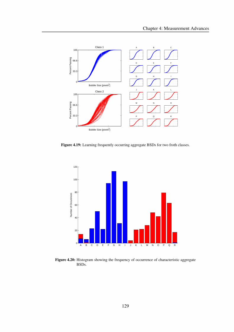
Chapter 4: Measurement Advances
0
33.3
66.6
100Class 1
Bubble Size [pixels2]
Per
cent
Pas
sing
0
33.3
66.6
100Class 2
Bubble Size [pixels2]
Per
cent
Pas
sing
A B C
D E F
G H I
J K L
M N O
P Q R
Figure 4.19: Learning frequently occurring aggregate BSDs for two froth classes.
A B C D E F G H I J K L M N O P Q R0
20
40
60
80
100
120
Num
ber
of O
ccur
ence
s
Figure 4.20: Histogram showing the frequency of occurrence of characteristic aggregate
BSDs.
129

Chapter 4: Measurement Advances
ring BSDs to use is heuristically driven. It should be large as possible such that there is a
suitable difference between the different classes identified. Nine classes have been used
here, but it is expected that using eight or ten classes would have similar results.
Once the set of characteristic aggregate BSDs has been determined, all of the samples in
the training data set are classified according to which of the characteristic aggregate BSDs
(A to R) they are most similar to. It is now possible to generate a histogram which shows
the frequency of occurrence of the characteristic aggregate BSDs for the froth classes.
Figure 4.20 shows such a histogram.
New video segments are classified by first calculating the aggregate BSD. Next, the ag-
gregate BSD is classified according to which of the characteristic BSDs (A to R) it is
most similar to. The histogram of characteristic BSDs is then used to determine the final
class allocation. For example, if the most similar characteristic BSD to the new sample
is ‘A’, then the new video segment will be classified as belonging to class 2 because there
are more class 2 occurrences of ‘A’ BSDs than class 1 occurrences of ‘A’ BSD. Alterna-
tively, if the new video segment is most similar to characteristic BSD ‘B’, then it will be
classified as belonging to class 1.
4.2.6 Dimensionality Reduced Aggregate BSD
An aggregate cumulative BSD is calculated for the video sample in the same manner
as outlined in Section 4.2.5. The aggregate cumulative bubble size distribution is then
binned into 50 bins. In effect this turns it into a fifty dimensional data point. This pro-
cedure is performed for multiple aggregate BSDs, resulting in a fifty dimensional point
cloud. The point cloud is then normalised to have zero mean and unit standard deviation.
After the normalisation process, principal component analysis is used to extract three
principal components. Three principal components are chosen because it allows for the
visualisation of the data. The data is then projected onto the three principal components
which results in the data being reduced to a three dimensional point cloud. This process
is done for a large number of training data samples two both froth classes.
New data can then be classified by converting the aggregate BSD to a fifty dimensional
point and then normalising using the same normalisation procedure mentioned previously.
130

Chapter 4: Measurement Advances
Next, the data is projected onto the principal component axes to result in a single three
dimensional point. A k nearest neighbour classifier is then used to classify the new data
point to determine which class it belongs to.
4.2.7 Frequently Occurring BSDs
The frequently occurring BSD algorithm is inspired by the work of Varma and Zisser-
man [68], but instead of finding image textons that occur frequently over an image, fre-quently occurring BSDs are determined that occur in the bubble size data.
The bubble size distributions are calculated for a random selection of frames from the
training data set. The number of frames selected needs to be representative of all the
bubble size distributions found in the data. Experimentation has shown that using 9000
samples is sufficient in most cases. The set of frequently occurring BSDs is determined
using an unsupervised hierarchical classification algorithm. This process is exactly the
same as the aggregate BSD algorithm, except that the input BSDs correspond to single
frames of video unlike the aggregate BSDs which correspond to many frames of video.
A sample video sequence can now have each individual frame classified according to
which of the frequently occurring BSDs it belongs. For example, a 10 frame sequence
could be reduced to {A, C, B, A, G, G, C, A, A,D}. These sequences can be converted
to distributions, which show the number of times a certain frequently occurring BSD
happens in the sample. Many of these distributions can be determined by taking a large
number of samples from the training data set. From this large set of distributions it is pos-
sible to use an unsupervised nearest neighbour clustering algorithm using the chi square
distance measure to determine a set of frequently occurring distributions for each froth
class. In this manner, associated with each froth class, is a set of distributions of fre-
quently occurring BSDs which are typical of samples from that class. Examples of such
distributions for two froth classes are shown in Figures 4.21 and 4.22.
New samples are classified by determining their corresponding distribution of frequently
occurring BSDs and seeing to which of the frequently occurring distributions it is most
similar (using the chi square distance measure). The sample will then be labelled accord-
ing to the class corresponding to the frequently occurring distribution to which it is most
similar.
131
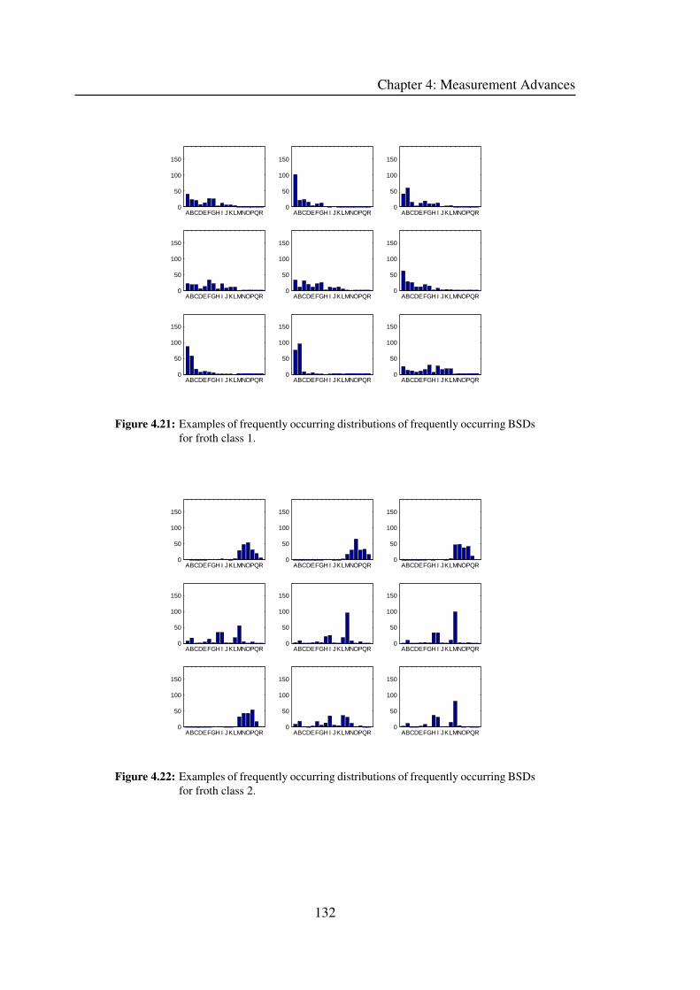
Chapter 4: Measurement Advances
ABCDEFGH I JKLMNOPQR0
50
100
150
ABCDEFGH I JKLMNOPQR0
50
100
150
ABCDEFGH I JKLMNOPQR0
50
100
150
ABCDEFGH I JKLMNOPQR0
50
100
150
ABCDEFGH I JKLMNOPQR0
50
100
150
ABCDEFGH I JKLMNOPQR0
50
100
150
ABCDEFGH I JKLMNOPQR0
50
100
150
ABCDEFGH I JKLMNOPQR0
50
100
150
ABCDEFGH I JKLMNOPQR0
50
100
150
Figure 4.21: Examples of frequently occurring distributions of frequently occurring BSDs
for froth class 1.
ABCDEFGH I JKLMNOPQR0
50
100
150
ABCDEFGH I JKLMNOPQR0
50
100
150
ABCDEFGH I JKLMNOPQR0
50
100
150
ABCDEFGH I JKLMNOPQR0
50
100
150
ABCDEFGH I JKLMNOPQR0
50
100
150
ABCDEFGH I JKLMNOPQR0
50
100
150
ABCDEFGH I JKLMNOPQR0
50
100
150
ABCDEFGH I JKLMNOPQR0
50
100
150
ABCDEFGH I JKLMNOPQR0
50
100
150
Figure 4.22: Examples of frequently occurring distributions of frequently occurring BSDs
for froth class 2.
132

Chapter 4: Measurement Advances
4.2.8 Results
4.2.8.1 Platinum Results
The results for classifying the platinum data set using the measurements outlined in Sec-
tions 4.2.3 to 4.2.7 are shown in Figure 4.23.
2 5 10 25 50 100 200 40050
60
70
80
90
100
Number of frames per sample
Per
cent
age
corr
ect c
lass
ifica
tion
Reduced Aggregate BSDAggregate BSDFrequently occuring BSDsBSD searchMean90% Passing80% PassingMedian (50% Passing)
Figure 4.23: Classification performance of bubble size distribution reduction techniques
on the platinum data set.
All of the results shown are the mean results for the measurements tested, usually over ten
to twenty test runs consisting of thousands of samples for both training and testing data
sets. It is important to note that a classification rate of 50% correct corresponds to that of
randomly assigning froth classes, and therefore is associated with very poor performance.
It is evident that the algorithms that make use of single value descriptors (mean, median
and p80) perform worse (best performance of 91.8%) than the complex bubble size de-
scriptors (worst performance of 91.5%). The increase in performance with the number of
frames in the video sample is not significant after ten frames for the single value descrip-
tors. The complex bubble size descriptors show a more consistent upwards trend with
increasing number of frames per video sample.
The dimensionality reduced aggregate BSD algorithm shows a downward trend when a
higher number of frames is used. More in-depth analysis of this phenomenon shows that
133

Chapter 4: Measurement Advances
these results are highly biased by one of the six sets of froth classes. It is suspected
that the reason for the decrease in performance is due to the large intra-class variance for
these two froth classes, resulting in the principal components not being aligned with the
inter-class variance as is desired.
4.2.8.2 Copper 2004 Results
The results for classifying the copper 2004 data set using the measurements outlined in
Sections 4.2.3 to 4.2.7 are shown in Figure 4.24.
2 5 10 25 50 100 200 40050
60
70
80
90
100
Number of frames per sample
Per
cent
age
corr
ect c
lass
ifica
tion
Reduced Aggregate BSDAggregate BSDFrequently Occurring BSDBSD search90% PassingMean80% PassingMedian (50% Passing)
Figure 4.24: Classification performance of bubble size distribution reduction techniques
on the copper 2004 data set.
The difference in performance between the single value descriptors (best performance of
71.3%) and complex bubble descriptors (worst performance of 75.3%) is much larger for
this set of copper froths than for platinum froths. The performance gap is greater than
twenty percent for large numbers of frames per sample. Again, an increase in the number
of frames processed results in a marked improvement in classification performance for
the complex bubble size descriptors. In fact, the number of frames processed has a more
significant effect on classification performance for copper froths (which have dynamic
BSDs) than for platinum froths.
The frequently occurring BSD algorithm performs better when the number of frames per
sample is large. The reason for this is likely to be that the distributions of frequently
134
Chapter 4: Measurement Advances
occurring BSDs are sparsely populated when the number of frames per sample is low.
This sparse population results in worse performance when using the chi square distance
measure.
4.2.9 Discussion
It is evident from the results that using complex bubble size descriptors results in greatly
improved classification performance. However, there is still the question of whether or
not the performance gains are worth the additional computational complexity of these
algorithms.
In the case of the platinum froth, the performance gain from using additional frames per
sample as well as the more complex descriptors is not particularly large. A more in-depth
investigation into the individual froth types being classified shows that the difference in
classification performance is mainly due to the difficulty distinguishing between one of
the six sets of froth types. If the difference between these froth types is not critical from
an operational point of view, it makes sense to use a single value descriptor such as the
p80.
For copper froths, the situation is very different. All of the single value descriptors have
performance values of less than 70% (50% correct classification corresponds to random
classification). This is largely due to the dynamic nature of the copper bubble size dis-
tribution. These dynamics are not well captured by a single value, as the amount of data
reduction taking place is too extreme. As a result of this, the single value descriptors are
almost meaningless as they fail to be able to distinguish between two visually different
froth types (which is exactly what one wants from the measurement in the first place). In
such a case, it is crucial to make use of the more complex bubble size descriptors.
The duration of the sample taken is another engineering trade off. The larger the number
of frames processed, the greater the classification performance. This is similar to most
sampling procedures where a larger number of samples results in more confidence of the
actual sample’s value. The down side of this is that it is often not appropriate to take
samples of long duration, especially when the sample is used for closed loop control
purposes. If the sample duration is too long, it is not always possible to respond in time
135

Chapter 4: Measurement Advances
to high frequency disturbances. It is for this reason that the maximum sample length used
is 400 samples. This corresponds to a 16 second long sample (at 25 frames a second).
It is important to note that the results shown here are for the specific copper and platinum
froths under investigation. They should not be generalised to all copper and platinum
froths. Experience has shown that platinum froths with dynamic bubble size distributions
do exist and that copper froths which don’t have dynamic BSDs also exist. In fact it is
important not to generalise the conditions found on one cell to the next cell in the same
bank.
When installing a machine vision system on a new site (or cell in an existing installation),
a series of tests should be performed to ensure that the appropriate bubble size measure
is being used. This is achieved by determining the range of bubble sizes present in the
froth being monitored, which in turn is achieved by adjusting input set-points (air, level,
reagents) to boundary regions of operation. Measurements of the entire bubble size dis-
tribution must be made for this selection of froth types. The discriminatory power of the
possible single value descriptors (mean, p50, p80, etc.) can then be tested to determine
whether they are providing meaningful information. This simple test will help to ensure
that the machine vision system is providing the controller/operator with useful informa-
tion which can be used to improve the flotation performance of the plant.
136

Chapter 4: Measurement Advances
4.3 Automatic Learning of Froth Classes
In this section, a method of automatically learning froth classes with dynamic bubble
size distributions is presented. It is particularly useful to be able to do this because the
manual identification of froth classes which exhibit dynamic bubble size distributions is
a particularly challenging task. This is because it is very difficult to identify both similar
and dissimilar froth classes because of the constantly changing froth surface. Being able
to automatically detect these classes will ensure consistency of results as well as saving
time and effort.
4.3.1 Algorithm Details
The algorithm is essentially a modification to the frequently occurring BSDs algorithm
presented in Section 4.2.7. As with the frequently occurring BSD algorithm, a large
sample of video data is taken, and the cumulative bubble size distributions which occur
frequently are identified using a furthest neighbour unsupervised clustering algorithm.
For this work, eight clusters are typically used. This value is chosen so that the number of
classes is small enough to ensure that there is still a visual difference between the images
from which the identified BSDs are generated. The mean cumulative bubble size distribu-
tion can then be calculated for each of the classes. The result is a set of cumulative bubble
size distributions which summarises the entire set of cumulative bubble size distributions
from the froth video segments. This resulting set of cumulative bubble size distributions
is known as the frequently occurring BSDs.
Using the frequently occurring cumulative bubble size distributions, it is possible to char-
acterise each video segment as a histogram. The histogram has the same number of bins
as the number of frequently occurring BSDs. The histogram shows the percentage of time
that the froth has a bubble size distribution similar to the frequently occurring bubble size
distributions. Figure 4.27 shows three examples of characteristic histograms of flotation
froths.
The chi-squared distance measure [49] can be used to provide a measure of dissimilarity
between the characteristic histograms of different froths. It is possible to create a dissim-
ilarity matrix for the entire data set of characteristic histograms of froth video segments.
137

Chapter 4: Measurement Advances
100
101
102
103
104
0
20
40
60
80
100
Bubble Size [pixels2]
Per
cent
age
Pas
sing
ABCDEFGH
Figure 4.25: Frequently occurring BSDs learnt from 9000 samples.
Figure 4.26: Example images of the froths represented by the cumulative BSDs in Fig-
ure 4.25.
A B C D E F G H0
10
20
30
40
50
60
Per
cent
age
of T
ime
Larger Bubbles Smaller Bubbles
A B C D E F G H0
10
20
30
40
50
60
Per
cent
age
of T
ime
Larger Bubbles Smaller Bubbles
A B C D E F G H0
10
20
30
40
50
60
Per
cent
age
of T
ime
Larger Bubbles Smaller Bubbles
Figure 4.27: The results of using unsupervised classification to determine three froth
classes. The labels of the histograms correspond to the labels of the BSDs in
Figure 4.25.
138

Chapter 4: Measurement Advances
This can be used in an unsupervised clustering algorithm (furthest-neighbour) to classify
the data set into classes with similar characteristic histograms.
The results from using the unsupervised clustering algorithm are shown in Figure 4.27.
Note that the labels of the bars in Figure 4.27 corresponds to the bubble size distributions
with the same labels in Figures 4.25 and 4.26. The characteristic histograms are clustered
into three froth classes. This number is chosen for two reasons: firstly, experience tells us
that flotation cells typically have between three to five different froth classes under normal
operating conditions and secondly, to maximise the amount of concentrate grade data per
froth class, which is important to ensure that statistically meaningful results are obtained.
4.3.2 Validation of Results
It is important to ensure that the resulting froth classes from the unsupervised clustering
algorithm are true froth classes and not artificial. The validation of the froth classes is
performed by examining the relationship between froth class, froth velocity and froth
concentrate grade. If the froth classes are just a random allocation, then the relationships
should all be the same. However, if the froth classes are real, different relationships should
emerge (provided that there are in fact different relationships between froth velocity and
concentrate grade for different froth classes.)
As will be shown in Chapter 6, while a linear model using the velocity measure alone is
not sufficient to explain the variation seen in the data, a model using the combination of
froth class and froth velocity is well suited to explain the variation observed in the data.
This suggests that it is likely that such a relationship should hold for other flotation cells
(such as the one used in the copper 2006 test work), and so it is reasonable to use the ex-
istence of a linear relationship to validate the froth classes identified by the unsupervised
clustering algorithm (see Section 7.3). If the this approach were to provide poor results
(ie. poor linear model fit), it would then be appropriate to move on to a non-linear model.
A brief overview of the statistical tests used for the comparison of regression lines from
different froth classes follows. For more detail, the reader is referred to [48, 49]. The fol-
lowing series of F-Tests are performed in order to determine whether or not the regression
lines are statistically different:
139

Chapter 4: Measurement Advances
1. F-Test for the comparison of data sets’ variance
2. F-Test for the comparison of the slopes of the regression lines
3. F-Test for the comparison of the intercepts of the regression lines
4. F-Test for the comparison of the mean of the regression lines.
An example of such a set of regression lines is shown in Figure 4.28 which corresponds
to a set of three froth classes which have been generated by randomly selecting their
membership. The values in Table 4.5 show the results from an analysis to determine
whether or not the regression lines from each of the randomly created froth classes are
statistically different. The values are all less than ninety-five percent. This indicates that
one cannot say with confidence that the lines are statistically different, and must therefore
accept the null hypothesis which is that there is no difference between these froth classes.
This is exactly what is to be expected from randomly allocated froth classes.
Figure 4.29 shows the resulting trends from using the fitting of a linear regression model
relating froth velocity to concentrate grade for each of the three froth classes determined
by the unsupervised clustering algorithm. It is evident from the figure that the trends have
different mean values, unlike the random allocation of froths in Figure 4.28.
Statistical analysis of the differences between these regression lines is show in Table 4.6.
All three of the regression lines are different from each other with at least 99.95% confi-
dence.
These results show that the techniques used here to automatically determine the froth
classes present in a set of videos of dynamic froths give meaningful results and not just a
random selection of froth classes.
140

Chapter 4: Measurement Advances
60 80 100 120 140 160 1800
5
10
15
20
25
30
Froth Velocity [mm/sec]
Cop
per
Con
cent
rate
Gra
de
Froth Class 1Froth Class 2Froth Class 3
Figure 4.28: Linear trends relating froth velocity to concentrate grade for three randomly
allocated froth classes.
Table 4.5: Summary of comparative statistics for three randomly allocated froth classes.
Froth Froth Confidence Confidence Confidence Confidence
Assay Class Class of Difference of Difference of Difference of Difference
A B in Slope in Intercept in Mean (Overall)
Copper [Cu]
1 2 84.08 10.37 55.23 84.08
1 3 53.04 34.01 66.95 66.95
2 3 56.61 29.64 64.78 64.78
141

Chapter 4: Measurement Advances
60 80 100 120 140 160 1805
10
15
20
25
30
35
Froth Velocity [mm/sec]
Cop
per
Con
cent
rate
Gra
de
Froth Class 1Froth Class 2Froth Class 3
Figure 4.29: Linear trends relating froth velocity to concentrate grade for three non-
randomly allocated froth classes.
Table 4.6: Summary of comparative statistics for three froth classes.
Froth Froth Confidence Confidence Confidence Confidence
Assay Class Class of Difference of Difference of Difference of Difference
A B in Slope in Intercept in Mean (Overall)
Copper [Cu]
1 2 7.89 99.91 99.95 99.95
1 3 5.11 99.99 100.00 100.00
2 3 61.40 99.91 99.96 99.96
142

Chapter 4: Measurement Advances
4.4 Texture Measures For Flotation
Numerous researchers have applied a variety of texture measures to the problem of clas-
sifying froth into discrete classes. For example: Nguyen [50] used the texture spectrum
for the classification of coal froth images, Moolman et al. [42] used spatial grey level
dependence matrices for the identification of copper froth classes and Bartolacci et al. [4]
used both wavelets and grey level co-occurrence matrices for predicting metallurgical
performance on zinc operations. What none of these researchers have provided is a good
reasons for why they have chosen the texture measurement they implemented over the
large number of available texture measures.
Texture measures such as those which are used for flotation froth image classification
have been designed with other textures in mind. The texture databases which are used
in their design are generally similar to the Brodatz photographic album [9]; they contain
numerous textures from a variety of sources, most of which do not look anything like
flotation froths. Since the texture measures have not been designed with flotation froth
classification in mind, it is important to test if the texture measures which are designed
for specific texture data sets will in fact perform well on flotation froth images.
This chapter begins by comparing the performance of a selection of the various texture
measurements that have been used by researchers for classifying flotation froth images as
well as a few other measures which have not been used. This is done using a Brodatz data
set similar to that which most of these algorithms will have been designed and tested on.
Next, the same texture measures are evaluated on their ability to classify flotation froth
images to see if their performance is consistent across the different data sets.
4.4.1 Texture Measures Tested
Numerous texture features were calculated for both the Brodatz and flotation froth data
sets. The list below summarises the texture measures and corresponding features which
were extracted. For details on the various texture algorithms, see Section 3.5.
• First Order StatisticsThe following features based on the first order statistics of the images were calcu-
143

Chapter 4: Measurement Advances
lated: mean, variance, standard deviation, RMS level, integral, skewness, kurtosis,
entropy and contrast.
• Greyscale Co-occurrence MatricesThe following features based on the greyscale co-occurrence matrix were calcu-
lated: energy, entropy, contrast, homogeneity, inverse difference moment and max-
imum probability. This was done for images with 256 grey levels, and for images
which had been reduced to 16 grey levels.
• Fourier RingsThe energy in each of the Fourier rings, the DC component and the total energy
were calculated for each image. This was done using three, six, nine and twelve
Fourier rings for both the magnitude and the power spectrum.
• Gabor Filter BankThe Gabor filter bank used had twenty oriented filters. Each of these was a resultant
feature.
• Autoregressive 2D PredictorAutoregressive predictors of order 1, 2 and 3 were calculated for each texture. This
resulted in four, five, and ten features respectively as the sigma value of the errors
is used as an additional feature.
• Laws’ Filter MasksLaws’ filter masks using the 3x3 and 5x5 kernels were applied to the texture images.
This resulted in eight and twenty four features respectively, as Laws suggests that
one of the filters is not used as a feature.
• Texture SpectrumThe texture spectrum was calculated for the textures. From the texture spectrum, the
features black-white symmetry, geometric symmetry, degree of direction, micro-
structure (horizontal, vertical and diagonal) and central symmetry were calculated.
This was done for images with 256 grey levels, and for images which had been
reduced to 16 grey levels.
• WaveletsA four-level wavelet decomposition was made on each image. The features ex-
144

Chapter 4: Measurement Advances
tracted were the mean and standard deviation of each of the sub-bands, as well as
wavelet histogram signatures for each of the sub-bands.
4.4.2 Classification of Froth Images
The texture measures listed in Section 4.4.1 were calculated for each of the images in the
flotation froth data set. For details of the data set used, see Section 3.10. The geometric
separability index was then calculated for the entire data set using each of the different
texture measures.
4.4.3 Results
The geometric separability index was used as a measure for determining how well the
texture measures could classify the set of 16793 images. As there are 18 classes of images,
the performance of a random class allocation would result in a geometric separability
index of 1/18 = 0.0556. An exhaustive search to determine which subset of features
resulted in the best classification of the data was performed for the texture measures that
had less than ten features. For those with more than ten features, an exhaustive search is
prohibitively large, and so only a limited number of subsets of features were tested. The
problem of feature subset selection is an active area of continuing research and beyond
the scope of this thesis. The results are shown in Table 4.7.
Table 4.7: Results from texture classification of flotation froth data set.
Texture Measure GSI Number of Features CommentsFirst Order Statistics 0.915 5
GSCOM 0.927 5
Fourier Rings 0.963 12 Magnitude Spectrum
Gabor Filter Bank 0.965 17 Magnitude Spectrum
Autoregressive 0.859 13 3rd Order
Laws’ Filter Masks 0.965 21 5x5 Kernel
Texture Spectrum 0.945 7 256 grey levels
Wavelets 0.900 7 3 Sub-bands
145

Chapter 4: Measurement Advances
4.4.4 Discussion
The results from the Brodatz data set show four texture features achieving perfect separa-
bility (the geometric separability index is shown in brackets):
1. autoregressive (1.0)
2. Laws’ filter masks (1.0)
3. texture spectrum (1.0)
4. wavelets (1.0).
From the results of the flotation froth data set the top four texture measures are (the geo-
metric separability index is shown in brackets):
1. texture spectrum (0.945)
2. Fourier rings (0.963)
3. Laws’ filter masks (0.965)
4. Gabor filters (0.965).
The trend that emerges is that the texture measures that exhibit the best performance on the
Brodatz data set are not necessarily the texture measures that exhibit the best performance
on the flotation froth data set. The two texture measures which appear in both sets of the
top four measurements are Law’s filter masks and the texture spectrum. This means that
results from texture measures for data sets such as the Brodatz album do not necessarily
indicate which texture measures are best suited to flotation froth images. In order to
determine how well a new texture measure is suited to classifying flotation froths, it must
be tested on an appropriate data set of flotation froth images.
In order for a texture measure to be viable for online, real-time analysis of flotation froths,
it needs to be relatively simple and computationally inexpensive. Because of this, it is
difficult to chose a best texture feature to use for froth flotation images based on the
results using the geometric separability index alone. The main reason for this is the high
dimensionality of the top two features for the flotation froth classification. Both the Gabor
filters and the Laws filter mask texture features have a very high number of features (17
and 21 respectively). Having such a high dimensional feature space is undesirable as one
needs an excessively large number of training data points to avoid the so called “curse of
146
Chapter 4: Measurement Advances
dimensionality”. In addition to this, both the Gabor filters and Laws’ filter masks require
applying large numbers of filters to the input image (17 and 21 respectively); this is a time
consuming task which might not outweigh the added benefit of using these methods.
As is often the case, the result is an engineering tradeoff. Here the tradeoff is between
the complexity of the texture method (time it takes to make the calculation), the dimen-
sionality of the output features (which affects the amount of training data required for
classification) and the performance of the texture measure. This suggests that it is best
to use either the Fourier ring method (which can have a variable number if rings, thus
changing the dimensionality of the feature space) or the texture spectrum method which
also performs well with only seven features.
4.5 Summary of Advances
This chapter has focussed on a variety of advances in the measurement of bubble size
distributions for flotation froths. The need for an algorithm which can accurately measure
bubble size distributions in flotation froths that contain both large and tiny bubbles has
been shown. An improvement to the watershed algorithm for bubble identification has
been discussed whereby detected blobs are classified according to their texture as being
either a single bubble or a collection of tiny bubbles. This classification stage allows
for multiple passes of the watershed algorithm using parameters optimised for different
bubble size detection each time.
Flotation froths which have dynamic bubble size distributions have been introduced and
various methods for reducing the complexity of their high dimensional bubble size distri-
butions have been investigated. For flotation froths which do not exhibit dynamic bubble
size distributions an engineering decision needs to be made as to whether the improve-
ment in classification that can be achieved by using the more complex dynamic bubble
size measurements (BSD Search, aggregate BSDs, frequently occurring BSDs, dimen-
sionality reduced BSD methods) is worth the additional computational complexity.
For flotation froths with dynamic bubble size distributions it is necessary to use the more
complex measurements. Reducing the bubble size distribution measurements to a single
value descriptor such as mean or p80 is often highly inappropriate and can result in the
loss of most of the information contained in the distribution.
147

Chapter 4: Measurement Advances
Sampling for increased durations has been shown to improve classification rates signifi-
cantly. For both data sets tested, classification rates of over 95% can be achieved when
using sample lengths of 100 frames (4 seconds).
A method of automatically learning dynamic froth classes has been proposed. This
method has been validated by showing that the resultant froth classes have statistically
different relationships between froth velocity and concentrate grade. This would not be
the case if the froth class allocation was random.
A variety of texture measures have been tested on a large data set of flotation froth images
associated with different minerals, ores and industrial operations. The results have shown
that numerous texture measures are well suited for the classification of these images.
Results have shown that Fourier ring and texture spectrum based texture measures are
best suited to flotation froth image classification for the flotation froth data set used here.
These measures can be expected to perform well on other flotation froth data sets.
148

Chapter 5
Machine Vision PerformanceRelationships – Platinum Data Set
This chapter addresses the fourth objective of this thesis: to show that a relationship exists
between machine vision measurements and the metallurgical performance (grade) that can
be readily utilised by industrial operations. To achieve this results are presented showing
the observed relationships between machine vision and metallurgical performance mea-
surements for the platinum data set.
For a machine vision system to be useful it is necessary to determine whether or not a re-
lationship exists between the observed froth descriptors (froth class, velocity, bubble size,
stability, etc.) and the metallurgical performance of the flotation cell being monitored.
The most common indicators of flotation cell performance are the concentrate grade and
the recovery of valuable minerals to the concentrate. Concentrate grade is a direct prop-
erty of the froth under a given set of conditions and does not require the analysis of flota-
tion pulp or tailings for its computation. Furthermore, from the machine vision point of
view, concentrate grade is a more appropriate performance indicator than recovery, since
the camera system only sees and analyses the very top layer of the flotation froth.
The recovery of valuables is defined as the proportion of minerals that exit the cell via
the concentrate, as opposed to via the tailings. Unlike concentrate grade, the calculation
of recovery requires the knowledge of feed grade, tailings grade, concentrate grade, feed
149

Chapter 5: Machine Vision Performance Relationships – Platinum Data Set
flow rate well as the mass flow rate of the concentrate stream. This makes it a more
difficult quantity to work with than concentrate grade. As such it will not be dealt with in
this thesis, but remains an important area for future research.
Once the existence of relationships between the machine vision measurements and the
concentrate grade have been established and their statistical significance checked, they
can potentially be used to improve the way that the flotation cell is operated. This can be
achieved by either informing personnel about the current concentrate grade of the flotation
cell or by implementing closed loop control on the flotation cell.
It is also important to investigate the relationship between machine vision measurements
and the feed to the flotation cell. If a change to the feed results in a change in machine
vision measurements, then the system can be used to detect when these changes occur and
the appropriate corrective action can be taken. It is also important to determine if observed
changes in concentrate grade are simply the result of the concentrate following changes
in the feed to the flotation cell or the result of improved performance of the flotation cell.
Three particular froth surface descriptors are considered as parameters to model the con-
centrate grade: froth velocity, bubble size and froth class data. Various combinations of
these measurements are also used. This chapter proceeds by showing the observed rela-
tionships between froth velocity, single value bubble size measurements, and concentrate
grade using both linear and non-linear models. Next, the froth classes of the platinum data
set and their method of identification are introduced. The observed relationships between
the froth classes, froth velocity and concentrate grade are presented and discussed. The
relationship between froth classes and flotation feed grade are investigated and discussed.
The chapter concludes with a summary and discussion of the results presented.
Because of the confidential nature of the platinum grade assays, all of the assay data
presented in this chapter has been normalised. While this ensures the confidentiality of
the data, it in no way changes the validity of the results presented.
150

Chapter 5: Machine Vision Performance Relationships – Platinum Data Set
5.1 Froth Velocity & Concentrate Grade
Froth velocity is an important measurement that can often be used to model the concen-
trate grade of a flotation cell. In simple terms, when the froth velocity increases there is
less time for drainage, and consequently the grade of the desirable material in the concen-
trate decreases while the grade of the gangue material in the concentrate increases.
Velocity measurements were made for each of the video segments for the samples in
the platinum data set. The relationship between the froth velocity measurements and the
concentrate grade measurements, taken at the same time, are shown in Figure 5.1 (with
a linear model fitted to the data). The use of linear models is not always appropriate for
modelling the relationship between froth velocity and concentrate. This is particularly
evident for the models relating PGMs, copper and chromite to the froth velocity, where
the residuals are not normally distributed but tend to sit in clusters either above or below
the fitted regression line. It may be more appropriate to use a non-linear model for this
data.
A number of non-linear models were fitted to the data to determine the best form of model.
The models tested include: 2nd and 3rd order polynomials, power relationships (axb and
axb + c) and exponential relationships (abx and abx + cdx). Results show that the best fits
are obtained when a non-linear power model of the form
y = a xb + c
is used (the complete set of results can be found in Appendix J). This is the form of the
non-linear model shown in Figure 5.2.
The non-linear models in Figure 5.2 provide a better fit than the linear models in Fig-
ure 5.1. The non-linear models typically account for between 51% and 80% of the vari-
ation seen in the concentrate grade, whereas the linear models (some of which violate
the assumption of normally distributed residuals) typically account for between 50% and
78%. Table 5.1 shows the differences in adjusted R2 values for the different models.
Although the linear model outperforms the non-linear model for some assays (Ni, Fe, S),
when this is the case, the additional variation in the data that is accounted for is minimal
(typically less than 2%). When the non-linear model outperforms the linear model, the
151

Chapter 5: Machine Vision Performance Relationships – Platinum Data Set
0 10 20 30 40 50 60 70 80 900
1000
2000
3000
4000
5000
6000
Froth Velocity [pixels/s]
PG
M N
orm
alis
ed C
onc
Gra
de [p
pm]
Individual SamplesRegression LineRegression Confidence LimitsSample Confidence Limits
Significance: 100.00 %Standard Error: 487.20Adj R Squared: 0.484R Squared: 0.504
0 10 20 30 40 50 60 70 80 900
2
4
6
8
10
12
Froth Velocity [pixels/s]C
u N
orm
alis
ed C
onc
Gra
de [%
] Individual SamplesRegression LineRegression Confidence LimitsSample Confidence Limits
Significance: 100.00 %Standard Error: 1.051Adj R Squared: 0.550R Squared: 0.568
0 10 20 30 40 50 60 70 80 900
2
4
6
8
10
Froth Velocity [pixels/s]
Ni N
orm
alis
ed C
onc
Gra
de [%
] Individual SamplesRegression LineRegression Confidence LimitsSample Confidence Limits
Significance: 100.00 %Standard Error: 0.546Adj R Squared: 0.538R Squared: 0.557
0 10 20 30 40 50 60 70 80 9060
65
70
75
80
85
Froth Velocity [pixels/s]
Fe
Nor
mal
ised
Con
c G
rade
[%] Individual Samples
Regression LineRegression Confidence LimitsSample Confidence Limits
Significance: 100.00 %Standard Error: 1.069Adj R Squared: 0.530R Squared: 0.549
0 10 20 30 40 50 60 70 80 900
2
4
6
8
10
12
Froth Velocity [pixels/s]
S N
orm
alis
ed C
onc
Gra
de [%
]
Individual SamplesRegression LineRegression Confidence LimitsSample Confidence Limits
Significance: 100.00 %Standard Error: 1.031Adj R Squared: 0.515R Squared: 0.534
0 10 20 30 40 50 60 70 80 900
10
20
30
40
50
60
Froth Velocity [pixels/s]
Cr 2O
4 Nor
mal
ised
Con
c G
rade
[%] Individual Samples
Regression LineRegression Confidence LimitsSample Confidence Limits
Significance: 100.00 %Standard Error: 2.899Adj R Squared: 0.770R Squared: 0.779
Figure 5.1: Linear relationship between froth velocity and concentrate grade for the plat-
inum data set.
152

Chapter 5: Machine Vision Performance Relationships – Platinum Data Set
10 20 30 40 50 60 70 80 900
1000
2000
3000
4000
5000
6000
Froth Velocity [pixels/s]
PG
M N
orm
alis
ed C
onc
Gra
de [%
] Individual SamplesRegression LineRegression Confidence LimitsSample Confidence Limits
Significance: 100.00 %Standard Error: 412.84Adj R Squared: 0.645R Squared: 0.674
10 20 30 40 50 60 70 80 900
2
4
6
8
10
12
Froth Velocity [pixels/s]
Cu
Nor
mal
ised
Con
c G
rade
[%] Individual Samples
Regression LineRegression Confidence LimitsSample Confidence Limits
Significance: 100.00 %Standard Error: 0.959Adj R Squared: 0.642R Squared: 0.670
10 20 30 40 50 60 70 80 900
2
4
6
8
10
Froth Velocity [pixels/s]
Ni N
orm
alis
ed C
onc
Gra
de [%
] Individual SamplesRegression LineRegression Confidence LimitsSample Confidence Limits
Significance: 99.96 %Standard Error: 0.570Adj R Squared: 0.519R Squared: 0.557
10 20 30 40 50 60 70 80 9060
65
70
75
80
85
Froth Velocity [pixels/s]
Fe
Nor
mal
ised
Con
c G
rade
[%] Individual Samples
Regression LineRegression Confidence LimitsSample Confidence Limits
Significance: 99.96 %Standard Error: 1.103Adj R Squared: 0.521R Squared: 0.559
10 20 30 40 50 60 70 80 900
2
4
6
8
10
12
Froth Velocity [pixels/s]
S N
orm
alis
ed C
onc
Gra
de [%
]
Individual SamplesRegression LineRegression Confidence LimitsSample Confidence Limits
Significance: 99.95 %Standard Error: 1.059Adj R Squared: 0.511R Squared: 0.550
10 20 30 40 50 60 70 80 900
10
20
30
40
50
60
Froth Velocity [pixels/s]
Cr 2O
4 Nor
mal
ised
Con
c G
rade
[%] Individual Samples
Regression LineRegression Confidence LimitsSample Confidence Limits
Significance: 100.00 %Standard Error: 2.777Adj R Squared: 0.798R Squared: 0.814
Figure 5.2: Non-linear relationship between froth velocity and concentrate grade for the
platinum data set.
153

Chapter 5: Machine Vision Performance Relationships – Platinum Data Set
Table 5.1: Adjusted R2 values for fitting linear and non-linear models to describe the
relationship between froth velocity and concentrate grade.
Model PGM Cu Ni Fe S Cr2O4
Linear 0.484 0.550 0.538 0.530 0.515 0.770
Non-Linear 0.645 0.642 0.519 0.521 0.511 0.798
additional variation in data accounted for is substantially larger (typically greater than
10%). These results suggest that a non-linear model is better for relating the froth velocity
to the concentrate grade for the platinum data set.
5.2 Bubble Size & Concentrate Grade
This section presents the results obtained when using a single value bubble size descrip-
tor to model the concentrate grade of the flotation cell being monitored. As discussed in
Chapter 4, the choice of bubble size measurement is critical to achieve optimal results.
Furthermore, using a single value bubble size descriptor is not always appropriate. How-
ever, the results for the classification of the platinum data set shown in Section 4.2.8 show
that it is possible to achieve 92% correct classification. This suggests that the use of a
single value bubble size descriptor for this data set is appropriate.
A test was performed to determine which single value bubble size descriptor was best
suited for modelling the concentrate grade of the froth. The test was performed using
both a linear and a non-linear model (the non-linear model has the same form as the one
presented in Section 5.1). The summarised results from the test are shown in Table 5.2,
with the complete set of results in Appendix H. The best results are shown in bold text for
both the linear and non-linear models.
Table 5.2: Average adjusted R2 values for fitting linear and non-linear models to rela-
tionship between various single value bubble size descriptors and concentrate
grade.
Model Mean p50 p60 p70 p80 p90
Linear 0.3993 0.2717 0.2677 0.2647 0.2626 0.3501
Non-Linear 0.4848 0.4394 0.4479 0.4570 0.5000 0.4760
154

Chapter 5: Machine Vision Performance Relationships – Platinum Data Set
For the linear models, the mean bubble size accounts for most of the variation seen in
the concentrate grade data. Therefore the linear models presented in this section show
the relationship between the mean bubble size and concentrate grade. Similarly, the p80
bubble size measurement is able to account for most of the variation in the data when a
non-linear power model is used, so the non-linear models presented in this section show
the relationship between the p80 bubble size and the concentrate grade.
Figure 5.3 shows the observed relationships between the mean bubble size measurement
and the concentrate grade assay values for the platinum data set with a linear model fitted
to the values. It is evident that the linear model is not appropriate, as the residuals are not
normally distributed around the model but tend to cluster in groups, either above or below
the model.
Figure 5.4 shows the results of a non-linear power model fitted to the p80 bubble size
data. The non-linear models explain a larger percentage of the variance in the data than
the linear models. The linear models account for between 23% and 65% of the variation
seen in the concentrate grade data, while the non-linear models account for between 31%
and 75% of the variation.
Table 5.3 shows the differences in adjusted R2 values for the different models.
Table 5.3: Adjusted R2 values for fitting linear and non-linear models to describe the
relationship between the bubble size and concentrate grade.
Model PGM Cu Ni Fe S Cr2O4
Linear 0.330 0.356 0.205 0.630 0.195 0.451
Non-Linear 0.369 0.367 0.349 0.702 0.105 0.711
It is evident from the results that a non-linear power model is better suited to explaining
the variation in the concentrate grade than a linear model, with an average increase of 7%
of the variation in the data being explained.
155

Chapter 5: Machine Vision Performance Relationships – Platinum Data Set
101
102
103
0
1000
2000
3000
4000
5000
6000
mean bubble size [pixels2]
PG
M N
orm
alis
ed C
onc
Gra
de [%
]
Individual SamplesRegression LineRegression Confidence LimitsSample Confidence Limits
Significance: 99.87 %Standard Error: 554.86Adj R Squared: 0.330R Squared: 0.357
101
102
103
0
2
4
6
8
10
mean bubble size [pixels2]C
u N
orm
alis
ed C
onc
Gra
de [%
] Individual SamplesRegression LineRegression Confidence LimitsSample Confidence Limits
Significance: 99.92 %Standard Error: 1.257Adj R Squared: 0.356R Squared: 0.382
101
102
103
0
2
4
6
8
10
mean bubble size [pixels2]
Ni N
orm
alis
ed C
onc
Gra
de [%
] Individual SamplesRegression LineRegression Confidence LimitsSample Confidence Limits
Significance: 98.82 %Standard Error: 0.716Adj R Squared: 0.205R Squared: 0.237
101
102
103
60
65
70
75
80
85
mean bubble size [pixels2]
Fe
Nor
mal
ised
Con
c G
rade
[%] Individual Samples
Regression LineRegression Confidence LimitsSample Confidence Limits
Significance: 100.00 %Standard Error: 0.948Adj R Squared: 0.630R Squared: 0.645
101
102
103
0
2
4
6
8
10
12
mean bubble size [pixels2]
S N
orm
alis
ed C
onc
Gra
de [%
] Individual SamplesRegression LineRegression Confidence LimitsSample Confidence Limits
Significance: 98.61 %Standard Error: 1.329Adj R Squared: 0.195R Squared: 0.227
101
102
103
0
10
20
30
40
50
60
mean bubble size [pixels2]
Cr 2O
4 Nor
mal
ised
Con
c G
rade
[%]
Individual SamplesRegression LineRegression Confidence LimitsSample Confidence Limits
Significance: 99.99 %Standard Error: 4.475Adj R Squared: 0.451R Squared: 0.473
Figure 5.3: Linear relationship between the mean bubble size and concentrate grade for
the platinum data set
156

Chapter 5: Machine Vision Performance Relationships – Platinum Data Set
101
102
103
0
1000
2000
3000
4000
5000
6000
p80 bubble size [pixels2]
PG
M N
orm
alis
ed C
onc
Gra
de [%
]
Individual SamplesRegression LineRegression Confidence LimitsSample Confidence Limits
Significance: 99.34 %Standard Error: 550.53Adj R Squared: 0.369R Squared: 0.420
101
102
103
0
2
4
6
8
10
12
p80 bubble size [pixels2]
Cu
Nor
mal
ised
Con
c G
rade
[%] Individual Samples
Regression LineRegression Confidence LimitsSample Confidence Limits
Significance: 99.31 %Standard Error: 1.275Adj R Squared: 0.367R Squared: 0.417
101
102
103
0
2
4
6
8
10
p80 bubble size [pixels2]
Ni N
orm
alis
ed C
onc
Gra
de [%
] Individual SamplesRegression LineRegression Confidence LimitsSample Confidence Limits
Significance: 99.08 %Standard Error: 0.663Adj R Squared: 0.349R Squared: 0.401
101
102
103
60
65
70
75
80
85
p80 bubble size [pixels2]
Fe
Nor
mal
ised
Con
c G
rade
[%] Individual Samples
Regression LineRegression Confidence LimitsSample Confidence Limits
Significance: 100.00 %Standard Error: 0.870Adj R Squared: 0.702R Squared: 0.726
101
102
103
0
2
4
6
8
10
12
p80 bubble size [pixels2]
S N
orm
alis
ed C
onc
Gra
de [%
] Individual SamplesRegression LineRegression Confidence LimitsSample Confidence Limits
Significance: 77.63 %Standard Error: 1.432Adj R Squared: 0.105R Squared: 0.177
101
102
103
0
10
20
30
40
50
60
p80 bubble size [pixels2]
Cr 2O
4 Nor
mal
ised
Con
c G
rade
[%]
Individual SamplesRegression LineRegression Confidence LimitsSample Confidence Limits
Significance: 100.00 %Standard Error: 3.320Adj R Squared: 0.711R Squared: 0.734
Figure 5.4: Non-linear relationship between p80 bubble size and concentrate grade for the
platinum data set
157

Chapter 5: Machine Vision Performance Relationships – Platinum Data Set
5.3 Froth Class & Concentrate Grade
The identification of froth classes has already been dealt with in Section 3.12. It is impor-
tant to remember that the detection of the froth classes could have been made in a number
of ways, each of with their own advantages and disadvantages. These include:
• by classification based on single value bubble size descriptors
• by classification according to dynamic bubble size based techniques such as re-
duced aggregate BSDs
• by classification based on texture measures.
Figure 5.5 shows four example images of the froth classes identified. The colour of the
border around each of the froth images is consistent with the colour of the concentrate
grade data that is presented in the figures that follow.
(a) Froth Class ‘A’. (b) Froth Class ‘B’.
(c) Froth Class ‘C’. (d) Froth Class ‘D’.
Figure 5.5: Sample images of the four froth classes identified on the Amandelbult first
rougher.
Figure 5.6 shows the observed relationships between the froth class and concentrate grade
of the cells being monitored. The figure also shows the resultant R2, adjusted R2, and
158

Chapter 5: Machine Vision Performance Relationships – Platinum Data Set
standard error values that are obtained when a model of the form
y = β0 + γ1C1 + γ2C2 + γ3C3 + ε
is used to relate the froth class to the concentrate grade data. Here βi and γi are the
regression coefficients and Ci are indicator variables that represent the froth classes [10].
Further results are presented in Tables 5.4 to 5.6, which show the number of samples
associated with each class, the mean and standard deviation of the assay values from the
results shown in Figure 5.6, and the results of Welch’s t-test calculations to determine
whether the observed values for the different froth classes are statistically different from
one another. Welch’s t-test is an adaptation of Student’s t-test [49] that can be used when
the two samples have different variances. Froth classes with statistically different mean
values are identified by bold text in Table 5.6.
Table 5.4: Number of samples for each platinum froth class.
Froth Class Number of Samples
A 8
B 6
C 6
D 6
Table 5.5: Mean and standard deviation values of the concentrate grade for the platinum
froth classes.
Froth PGM PGM Copper Copper Nickel Nickel
Class Mean Std Dev Mean Std Dev Mean Std Dev
A 2288 413 3.87 1.02 5.40 0.24
B 1459 227 1.63 0.33 3.84 0.34
C 2008 377 3.04 0.38 4.58 0.31
D 2847 809 5.07 1.72 5.76 0.42
Froth Iron Iron Sulfur Sulfur Chromite Chromite
Class Mean Std Dev Mean Std Dev Mean Std Dev
A 65.29 1.05 6.35 1.04 16.36 0.43
B 67.21 0.92 3.62 0.64 30.01 3.28
C 64.09 0.74 4.87 0.40 16.51 0.64
D 63.84 0.81 6.80 0.99 16.45 0.92
Table 5.6 shows that there is a significantly different mean concentrate grade value be-
tween the different froth classes for the majority of froth class/assay combinations. This
159

Chapter 5: Machine Vision Performance Relationships – Platinum Data Set
A B C D0
1000
2000
3000
4000
5000
Froth ClassPG
M N
orm
alis
ed C
once
ntra
te G
rade
[ppm
]
Std Err: 497.477Adj R2: 0.462R2: 0.526
A B C D0
2
4
6
8
10
Froth ClassC
u N
orm
alis
ed C
onc
Gra
de [%
]
Std Err: 1.028Adj R2: 0.569R2: 0.621
A B C D0
2
4
6
8
10
Froth Class
Ni N
orm
alis
ed C
onc
Gra
de [%
]
Std Err: 0.328Adj R2: 0.833R2: 0.853
A B C D60
65
70
75
80
Froth Class
Fe
Nor
mal
ised
Con
c G
rade
[%]
Std Err: 0.904Adj R2: 0.663R2: 0.704
A B C D0
2
4
6
8
10
12
Froth Class
S N
orm
alis
ed C
onc
Gra
de [%
]
Std Err: 0.836Adj R2: 0.681R2: 0.720
A B C D0
10
20
30
40
50
Froth Class
Cr 2O
4 Nor
mal
ised
Con
c G
rade
[%] Std Err: 1.668
Adj R2: 0.924R2: 0.933
Figure 5.6: Relationships between froth class and normalised concentrate grade for the
platinum data set.
160

Chapter 5: Machine Vision Performance Relationships – Platinum Data Set
result is significant from an operational point of view, as it means that plant personnel
can use froth class information to infer the concentrate grade of the flotation cell being
monitored. Furthermore, analyses can be performed to determine the optimal operational
froth class for the cell being monitored. Once this has been done, personnel can be alerted
when the flotation cell is not operating in the desired froth class, and corrective action can
be taken.
Table 5.6: Summary of the statistical confidence of differences in the mean value of the
concentrate for various mineral and froth class combinations, using Welch’s
t-test.
Class 1 Class 2 PGM Copper Nickel Iron Sulfur Chromite
A B 99.98 99.94 100.00 99.66 99.99 99.98A C 93.74 78.45 99.95 97.27 99.48 35.93
A D 83.36 83.45 89.45 98.74 57.68 16.00
B C 100.00 98.42 99.73 99.99 99.65 99.98B D 99.52 99.32 100.00 99.99 99.99 99.99C D 96.33 94.50 99.96 41.18 99.69 10.28
The results in Table 5.7 show that a simple model based solely on the classification of the
flotation froth can account for between 46% and 83% of the variation in the concentrate
grade data.
Table 5.7: Adjusted R2 values for fitting a linear model to describe the relationship be-
tween froth class and concentrate grade.
Model PGM Cu Ni Fe S Cr2O4
Froth Class 0.462 0.569 0.833 0.663 0.681 0.924
5.4 Froth Class, Velocity & Concentrate Grade
In this section a combination of froth velocity and froth class measurements is used to
model concentrate grade, to determine if better results can be obtained using multiple
parameters. The concentrate grade is modelled as a function of froth class and froth
velocity. The results show that there are generally no significant relationships relating
the froth class and velocity to the concentrate grade for the platinum data set. Figure 5.7
161

Chapter 5: Machine Vision Performance Relationships – Platinum Data Set
shows the results for modelling the copper grade. These results are typical of the other
assays, the rest of which can be seen in Appendix G.
0 10 20 30 40 50 60 70 80 900
2
4
6
8
10
12
Froth Velocity [pixels/s]
Cu
Nor
mal
ised
Con
c G
rade
[%] Individual Samples Significance: 25.52 %
Standard Error: 1.089Adj R Squared: −0.144R Squared: 0.019
(a) Froth Class ‘A’.
0 10 20 30 40 50 60 70 80 900
2
4
6
8
10
12
Froth Velocity [pixels/s]C
u N
orm
alis
ed C
onc
Gra
de [%
] Individual Samples Significance: 10.44 %Standard Error: 0.365Adj R Squared: −0.244R Squared: 0.005
(b) Froth Class ‘B’.
0 10 20 30 40 50 60 70 80 900
2
4
6
8
10
12
Froth Velocity [pixels/s]
Cu
Nor
mal
ised
Con
c G
rade
[%] Individual Samples Significance: 37.38 %
Standard Error: 0.414Adj R Squared: −0.169R Squared: 0.065
(c) Froth Class ‘C’.
0 10 20 30 40 50 60 70 80 900
2
4
6
8
10
12
Froth Velocity [pixels/s]
Cu
Nor
mal
ised
Con
c G
rade
[%] Individual Samples
Regression LineRegression Confidence LimitsSample Confidence Limits
Significance: 96.86 %Standard Error: 1.006Adj R Squared: 0.657R Squared: 0.725
(d) Froth Class ‘D’.
Figure 5.7: Relationship between froth class, froth velocity and concentrate grade for the
platinum data set.
Due to the short nature of the test work campaign, there is only a narrow range of veloc-
ities associated with each froth class. This is the likely reason for not observing trends
relating the froth velocity to concentrate grade for the different froth classes.
Another limitation which prevents the determination of any significant relationship be-
tween froth velocity, froth class, and concentrate grade is the limited number of data
points associated with each froth class. The results from this analysis should therefore be
considered inconclusive, with further tests being required to determine if a relationship
exists. These tests would need to ensure that both more samples are collected and that a
greater range of froth velocities are sampled for the different froth classes.
162

Chapter 5: Machine Vision Performance Relationships – Platinum Data Set
5.5 Bubble Size, Velocity & Concentrate Grade
Another possible combination of froth surface descriptors for modelling the concentrate
grade is that of bubble size and froth velocity. When a linear model based on these two
measurements is used to model the concentrate grade, the results show that the addition
of the bubble size parameter only carries a significance of 45.8% (ie. not significant), as
shown is in Table 5.8. The resultant model has not been plotted in a figure because of the
difficulty of plotting a multiple linear regression model in two dimensions.
Table 5.8: Summary of the significance of independent variables for modelling concen-
trate grade as a linear function of mean bubble size and velocity.
Model Parameter Significance
Intercept 91.6
Mean Bubble Size 45.8
Froth Velocity 95.6
These results are not in agreement with those presented in Section 5.2, which show that
a significant relationship exists between bubble size and concentrate grade. This discrep-
ancy occurs because the bubble size and velocity measurements are co-linear, as is seen
in Figure 5.8. The co-linearity between bubble size and froth velocity means that the two
model parameters are not independent (a requirement for linear regression models) and
explains why the addition of the bubble size measurement does not add any new informa-
tion to the regression model.
The most likely reason for the co-linearity of the two measurements is the short duration
of the test campaign, where adjustments were made to the froth depth in order to change
the visible top-of-froth state. Although it is possible that there bubble size and froth
velocity are always co-linear, it is suspected that the short duration and execution of the
test campaign are the main contributing factors.
163

Chapter 5: Machine Vision Performance Relationships – Platinum Data Set
101
102
103
10
20
30
40
50
60
70
80
Fro
th V
eloc
ity [p
ixel
s/s]
Mean Bubble Size [pixels2]
Figure 5.8: Co-linear relationship between froth velocity and mean bubble size for the
platinum data set.
164

Chapter 5: Machine Vision Performance Relationships – Platinum Data Set
5.6 Feed Grade
This section examines the relationships between the feed to the cell and the froth class
observed by the machine vision system. The reason for examining the feed is twofold:
firstly, it is important to see if the cell performance is correlated with the feed, and sec-
ondly, to explore the potential that the froth class can provide information about the feed
to the cell.
Figure 5.9 show the observed relationships between froth classes and feed grade of the
cells being monitored. Table 5.9 shows the results of t-test calculations to determine
whether the observed values for the different froth classes are statistically different from
one another. Froth classes with statistically different mean values are identified by bold
text.
Table 5.9: Summary of the statistical confidence of differences in the mean value of the
feed for various mineral and froth class combinations using Welch’s t-test.
Class 1 Class 2 PGM Copper Nickel Iron Sulfur Chromite
A B 38.05 63.75 38.40 87.99 18.16 62.31
A C 50.70 44.32 4.56 43.39 55.85 90.46
A D 71.72 89.20 94.02 68.93 90.78 43.05
B C 76.86 78.20 37.53 99.97 48.05 99.79B D 87.62 92.89 88.56 17.03 84.88 1.78
C D 33.89 62.35 94.43 89.94 17.07 91.39
Except for the iron and chromite for classes ‘B’ and ‘C’, there is no statistical difference
between the mean values of the different froth classes. This means that the variations seen
in the concentrate grade are not a function of the feed to the flotation cell.
Figure 5.10 shows the relationship between the p80 bubble size and the feed to the flota-
tion cell being monitored. As is the case for the froth classes, no significant relationship
relates the p80 bubble size to the feed assay values, indicating the froth bubble size is not
dependent on the assay grade of the feed.
The froth class and bubble size variations are therefore likely to have arisen as a result
of feed independent conditions (such as air, level, reagents, etc.), and they can probably
be manipulated by adjusting these conditions. How specific froth class/bubble size com-
binations can be achieved by manipulating these parameters is beyond the scope of this
thesis.
165

Chapter 5: Machine Vision Performance Relationships – Platinum Data Set
A B C D0
10
20
30
40
50
60
70
Froth Class
PG
M N
orm
alis
ed F
eed
Gra
de [p
pm]
A B C D0.08
0.09
0.1
0.11
0.12
Froth ClassC
u N
orm
alis
ed F
eed
Gra
de [%
]
A B C D0.7
0.72
0.74
0.76
0.78
0.8
0.82
Froth Class
Ni N
orm
alis
ed F
eed
Gra
de [%
]
A B C D80
85
90
95
100
105
Froth Class
Fe
Nor
mal
ised
Fee
d G
rade
[%]
A B C D
0.1
0.15
0.2
0.25
Froth Class
S N
orm
alis
ed F
eed
Gra
de [%
]
A B C D105
110
115
120
125
130
135
140
145
Froth Class
Cr 2O
4 Nor
mal
ised
Fee
d G
rade
[%]
Figure 5.9: Relationships between froth class and normalised feed grade for the platinum
data set. (Note that although there appears to be different numbers of samples
in some of the graphs, this is not the case. Some of the samples have the same
assay values.)
166

Chapter 5: Machine Vision Performance Relationships – Platinum Data Set
101
102
103
0
10
20
30
40
50
60
70
p80 Bubble Size
PG
M N
orm
alis
ed F
eed
Gra
de [p
pm]
101
102
103
0.08
0.09
0.1
0.11
0.12
0.13
p80 Bubble Size
Cu
Nor
mal
ised
Fee
d G
rade
[%]
101
102
103
0.7
0.72
0.74
0.76
0.78
0.8
0.82
p80 Bubble Size
Ni N
orm
alis
ed F
eed
Gra
de [%
]
101
102
103
80
85
90
95
100
105
p80 Bubble Size
Fe
Nor
mal
ised
Fee
d G
rade
[%]
101
102
103
0.05
0.1
0.15
0.2
0.25
p80 Bubble Size
S N
orm
alis
ed F
eed
Gra
de [%
]
101
102
103
100
110
120
130
140
150
p80 Bubble Size
Cr 2O
4 Nor
mal
ised
Fee
d G
rade
[%]
Figure 5.10: Relationships between p80 bubble size and normalised feed grade for the
platinum data set.
167

Chapter 5: Machine Vision Performance Relationships – Platinum Data Set
These results indicate that the observed froth classes (or p80 bubble size) are not a func-
tion of the feed, but are in fact a measure of the performance (concentrate grade) of the
flotation cell.
5.7 Summary & Discussion
The results presented in this chapter have shown that relationships exist between:
• froth velocity and concentrate grade
• froth bubble size and concentrate grade
• froth class and concentrate grade.
The relationships between froth velocity and concentrate grade and froth bubble size and
concentrate grade have been show to be best modelled with a non-linear function of the
form
y = a xb + c.
For the relationship between the froth classes and concentrate grade, a linear model has
been shown to be sufficient.
The results from this chapter are summarised in Table 5.10. It shows the adjusted R2
values for each of the variables used to model the concentrate grade of the platinum data
set. It is evident that by using a combination of froth velocity and froth class it is possible
to account for the greatest percentage of the variation seen in the concentrate grade. This
is true for all except for the iron assay, where the bubble size accounts for an additional
4% of the variation.
Table 5.10: Adjusted R2 values for fitting various models to concentrate grade.
Model PGM Cu Ni Fe S Cr2O4
Froth Velocity (Linear) 0.484 0.550 0.538 0.530 0.515 0.770
Froth Velocity (Non-Linear) 0.645 0.642 0.519 0.521 0.511 0.798
Bubble Size (Linear) 0.330 0.356 0.205 0.630 0.195 0.451
Bubble Size (Non-Linear) 0.369 0.367 0.349 0.702 0.105 0.711
Froth Class (Linear) 0.462 0.569 0.833 0.663 0.681 0.924
168

Chapter 5: Machine Vision Performance Relationships – Platinum Data Set
The results from the direct combination of froth velocity and froth class show no im-
provement to the model relating these measurements to concentrate grade. It is suspected
that the reason for this is largely due to the limited nature of the data set, which does not
have a sufficiently large range of froth velocities for the different froth classes. However,
there are indications (see Figure 5.7d) that with more data the combination of these two
measurements could explain an even greater percentage of the variation in the data.
Analysis of the feed to the flotation cell has discovered no significant relationship between
the feed and the froth class present on the surface. Further analysis shows no significant
relationship between the feed to the flotation cell and the mean bubble size.
The results suggest that the observed relationships can be used by plant personnel to
improve the performance (grade) of the flotation cell. By making the appropriate adjust-
ments, the flotation cell’s froth velocity and froth class can be changed so that it operates
in an optimal regime (froth class and velocity combination).
Although the models presented do not account for all of the scatter seen in the concentrate
data for the platinum data set, it is important to realise that it is the mean concentrate grade
value under a specific regime that is important. This is largely due to the combination of
variability in feed and long residence times of the flotation cell. Even if it were possible to
account for all of the variation seen in the data, it would not be possible to make changes
to the flotation cell quickly enough to ensure that optimal performance is achieved. In fact,
it is likely that if such rapid changes to the process parameters (air, level and reagents)
were made the result would be an unstable operation of the flotation cell, with decreased
performance.
169

Chapter 5: Machine Vision Performance Relationships – Platinum Data Set
170

Chapter 6
Machine Vision PerformanceRelationships – Molybdenum Data Set
This chapter presents the results from test work carried out on the molybdenum circuit at
Kennecott Utah Copper Concentrator in February 2006. The chapter continues to address
the fourth objective this thesis: to show that a relationship exists between machine vision
measurements and the metallurgical performance (grade), and that this relationship can
be readily utilised by industrial operations.
The chapter begins by presenting and discussing the observed relationship between the
froth velocity and concentrate grade for the molybdenum data set. Next, it discusses why
it is not feasible to make accurate bubble size measurements for the flotation froths in
the molybdenum data set. Texture measures are presented as an appropriate alternative
measurement to use when accurate bubble size measurements cannot be made. Next, the
observed relationships between the froth classes (based on texture measurements), froth
velocity, and the concentrate grade are presented.
Finally, the observed relationships between the froth classes, feed, and process operat-
ing conditions are presented and discussed. The chapter ends with a discussion on the
observed relationships between the machine vision measurements and the concentrate
grade, and suggests how the results may be used to improve the performance of industrial
flotation cell operation.
171

Chapter 6: Machine Vision Performance Relationships – Molybdenum Data Set
6.1 Froth Velocity & Concentrate Grade
A linear regression model was used to model the concentrate grade using the froth velocity
as the independent parameter. Figure 6.1 shows the observed relationships between froth
velocity and the assay values of the concentrate. No significant relationship between froth
velocity and magnesium oxide grade was found.
0 50 100 1500
5
10
15
Cop
per
[Cu]
in C
onc
Froth Velocity [mm/sec]
R Squared: 0.403Adj R Squared: 0.392Standard Error: 1.818Significance: 100.00 %Individual Samples
Regression LineRegression Confidence LimitsSample Confidence Limits
0 50 100 1500
5
10
15
Iron
[Fe]
in C
onc
Froth Velocity [mm/sec]
R Squared: 0.596Adj R Squared: 0.589Standard Error: 1.410Significance: 100.00 %Individual Samples
Regression LineRegression Confidence LimitsSample Confidence Limits
0 50 100 1500
5
10
15
20
Mag
nesi
um O
xide
[MgO
] in
Con
c
Froth Velocity [mm/sec]
R Squared: 0.045Adj R Squared: 0.027Standard Error: 2.005Significance: 87.64 %Individual Samples
0 50 100 1500
20
40
60
80
100
120
Mol
ybde
num
Dis
ulfid
e [M
oS2] i
n C
onc
Froth Velocity [mm/sec]
R Squared: 0.448Adj R Squared: 0.437Standard Error: 15.844Significance: 100.00 %Individual Samples
Regression LineRegression Confidence LimitsSample Confidence Limits
Figure 6.1: Results showing the observed relationships between froth velocity and con-
centrate assay values with linear models fitted.
Analysis of the residuals of these linear models reveals that the residuals for the copper
model are not normally distributed. This means that the assumptions under which the
model is based are invalid. Similar problems occur for the molybdenum disulfide model,
which has decreasing residual values with increasing froth velocity. These results show
that the observed relationship should be disregarded and suggest that a non-linear model
172

Chapter 6: Machine Vision Performance Relationships – Molybdenum Data Set
may be more appropriate for explaining the relationship. The plots of residuals for all of
the trends shown in Figure 6.1 can be found in Appendix E.
As in Chapter 5, a non-linear power model of the form
y = a xb + c
was used to model the relationship between the froth velocity and the concentrate grade.
The results are shown in Figure 6.2.
0 50 100 1500
5
10
15
Cop
per
[Cu]
in C
onc
Froth Velocity [mm/sec]
Individual SamplesRegression LineRegression Confidence LimitsSample Confidence Limits
Significance: 100.00 %Standard Error: 1.849Adj R Squared: 0.383R Squared: 0.406
0 50 100 1500
5
10
15
Iron
[Fe]
in C
onc
Froth Velocity [mm/sec]
Individual SamplesRegression LineRegression Confidence LimitsSample Confidence Limits
Significance: 100.00 %Standard Error: 1.429Adj R Squared: 0.585R Squared: 0.601
0 50 100 1500
5
10
15
20
Mag
nesi
um O
xide
[MgO
] in
Con
c
Froth Velocity [mm/sec]
Individual Samples Significance: 94.01 %Standard Error: 1.945Adj R Squared: 0.103R Squared: 0.137
0 50 100 1500
20
40
60
80
100
120
Mol
ybde
num
Dis
ulfid
e [M
oS2] i
n C
onc
Froth Velocity [mm/sec]
Individual SamplesRegression LineRegression Confidence LimitsSample Confidence Limits
Significance: 100.00 %Standard Error: 16.033Adj R Squared: 0.435R Squared: 0.456
Figure 6.2: Results showing the observed relationships between froth velocity and con-
centrate assay values with non-linear models fitted.
A summary of the adjusted R2 values for both the linear and non-linear models is shown
in Table 6.1.
173

Chapter 6: Machine Vision Performance Relationships – Molybdenum Data Set
Table 6.1: Adjusted R2 values when froth velocity is used to model the concentrate grade.
Cu Fe MgO MoS2
Linear Model 0.392 0.589 0.027 0.437Non-Linear Model 0.383 0.585 0.103 0.435
It is evident from these results that the non-linear model does not differ greatly from
the linear model. In fact, the non-linear model has an almost linear relationship for the
range of froth velocities measured. Furthermore, the adjusted R2 values for the non-linear
models are generally lower than those of the linear models. This is a consequence of an
increase in the degrees of freedom in the model with no substantial increase in the amount
of variability in the data being accounted for. Froth velocity alone is not particularly suited
to the modelling of concentrate grade, and a combination of measurements might perform
better.
6.2 Bubble Size Measurement
Figure 6.3 shows four example images from the video footage collected from the molyb-
denum third rougher cell. Visual inspection of the molybdenum froth suggests that it is
ill-suited to being segmented using the watershed algorithm (or most available bubble size
measurements for that matter). One of the images (Figure 6.3a) is suitable for segmen-
tation. The other three have specific problems which make the accurate measurement of
the bubble size distribution unfeasible. These problems are explained below.
6.2.1 Visible Pulp Areas
Some of the froth images have areas which contain not bubbles but pulp (Figure 6.3b
and 6.3c). Since the watershed algorithm is designed for flotation froths which consist
only of bubbles, it is expected that these regions of pulp will result in poor segmentation
of the molybdenum froth images. Other froth segmentation algorithms which also rely
on gradient based methods [21, 72, 73] will give poor results for the same reason. This is
further complicated by the fact that the pulp areas reflect light and appear as highlights.
174

Chapter 6: Machine Vision Performance Relationships – Molybdenum Data Set
(a) Froth well suited to watershed seg-
mentation.
(b) Froth with visible areas of pulp
(c) Froth with visible areas of pulp and
motion blur
(d) Transparent Froth
Figure 6.3: Sample images of different froth conditions which can be difficult to segment.
This is a problem because the gradient based methods assume that the highlights in the
image are the centres of individual bubbles (see Chapter 3 for details on the watershed
algorithm).
6.2.2 Motion Blur
Figure 6.3c illustrates the problem of motion blur. Because of the small size of the bubbles
on the molybdenum circuit and their relatively high froth velocity, motion blur occurs.
This blurring prevents the watershed algorithm from providing an accurate bubble size
distribution of the froth. While the blurring could be reduced by using improved camera
and lighting systems, it is important to note that it is a limitation of the data set which is
used in this thesis.
175

Chapter 6: Machine Vision Performance Relationships – Molybdenum Data Set
6.2.3 Transparent Froth
The final problem is that certain flotation froths are sometimes transparent in nature.
This transparent nature of the bubbles is not immediately obvious from still images (Fig-
ure 6.3d), but is evident when they are directly observed. Such froths are also unsuitable
for segmentation using the watershed algorithm (or other gradient based methods) as it
relies on a decreasing greyscale value from the bubble highlight to the bubble boundary.
A smooth gradient does not exist for the bubble images in froths such as this: it is possible
to see the second layer of bubbles underneath the top layer, which results in an irregular
profile from the centre to the edge of the bubbles in the image.
The problem of transparent froth is not limited to the molybdenum data set. It is known
to occur in other flotation systems as well. Figure 6.4 shows an example from the froth
image data set presented in Chapter 3. Figure 6.5 shows the typical greyscale profiles
through a bubble for a transparent and an opaque froth.
Figure 6.4: An example image of a transparent froth from a phosphate concentrator.
6.2.4 Poor Segmentation Results
Figure 6.6 shows the results of an attempt to segment the images in Figure 6.3 using the
watershed algorithm. It is evident that the watershed algorithm does not perform well at
segmenting the bubbles in the molybdenum data set. This is because numerous individ-
ual bubbles have been erroneously over-segmented into multiple regions, collections of
tiny bubbles are under-segmented, and areas of pulp are over-segmented and erroneously
combined with individual bubbles.
176

Chapter 6: Machine Vision Performance Relationships – Molybdenum Data Set
(a) (b)
Figure 6.5: (a) Typical profile of a bubble in a transparent froth. (b) Typical profile of a
bubble in an opaque froth.
Figure 6.6: Attempted watershed segmentation of the images in Figure 6.3.
6.3 Texture Measures for Froth Identification
As shown in the previous section, accurate bubble size measurements are not possible for
the molybdenum data set. Texture is an alternative measure which is related to the bubble
size distribution for flotation froths. In fact, previous researchers [50] have shown that it
177

Chapter 6: Machine Vision Performance Relationships – Molybdenum Data Set
is possible to estimate the mean bubble size of a flotation froth using the combination of
a non-linear model and appropriate texture measurements.
Texture measures alone typically take the form of multidimensional data which are often
difficult to interpret as they do not directly represent any obvious physical characteristics
of the image they were calculated from. For this reason, researchers typically use the
texture measurements to identify the froth as belonging to one of a set of froth classes [31,
42, 50, 52].
Chapter 4 has shown which texture measures are suited to the identification of flotation
froth classes. Results of similar tests are presented here to see if the best texture measures
for the molybdenum data set are consistent with the results in Chapter 4. To achieve this,
two different classification methods are used to both train and test a variety of texture
measures on the molybdenum data set.
The first classifier used is a k nearest neighbour classifier (KNN) and the second a Gaus-
sian mixture model (GMM) classifier. For details of the classification methods the reader
is referred to Section 3.6. The reasoning behind choosing these two classifiers is that they
represent two different approaches, the KNN requiring large amounts of training data to
be kept for the classification stage, and the GMM having reduced the training data to a
minimal data model.
The best performance data is summarised in Table 6.2. For an in-depth view of the results
showing the classification performance for the classifier using different numbers of neigh-
bours and Gaussian centres, see Appendix D. From these results it is clear that a number
of texture measures can be used to achieve very high (> 95%) classification results for the
molybdenum data set. The Fourier ring method achieves the best classification results.
Example images of the four different froth classes which can be successfully identified
using texture measures are shown in Figure 6.7. The border colours of the different froth
class images are consistent with the colours used to present the observed relationships
between the froth classes and concentrate grade, feed grade, and process conditions later
in the chapter.
Thus, despite not being able to accurately measure the bubble size distribution of the
flotation froths, it is possible to classify the froths according to texture measures which
give an indirect measure of the bubble size.
178

Chapter 6: Machine Vision Performance Relationships – Molybdenum Data Set
Table 6.2: Results from classification of molybdenum data set using a variety of texture
measures.
Texture GMM Classification KNN Classification
Measure Results Results
Fourier rings 99.52 99.71
Texture spectrum 97.28 98.09
Laws’ filter masks 96.72 98.70
Gabor filters 96.56 97.83
Autoregressive 95.93 98.42
GSCOM 90.36 93.78
Statistics 83.19 94.20
Figure 6.7: Sample images of the different froth classes that can be identified using texture
measures.
6.4 Froth Class & Concentrate Grade
It has been shown that the froth velocity measurement accounts for 39%, 59% and 44%
of the variation in the copper, iron and molybdenum disulfide in the concentrate grade
179

Chapter 6: Machine Vision Performance Relationships – Molybdenum Data Set
respectively. This section presents the observed relationship between the froth class and
the concentrate grade of the flotation cell being monitored, to determine if the froth class
is better able to account for the variability observed in the concentrate grade data.
Figure 6.8 shows the observed relationships between the froth classes and the concentrate
grade of the flotation cell. Table 6.3 shows the mean assay values from the results shown
in Figure 6.8. Table 6.4 gives the statistical confidence that there is a true difference
between the mean values of the froth classes for each of the assays performed (calculated
using Welch’s t-test for samples with unequal variances). Values which have greater than
95% confidence of different mean values are highlighted.
A B C D0
2
4
6
8
10
Cop
per
[Cu]
Con
cent
rate
Gra
de
Froth Class
Std Err: 1.341Adj R2: 0.684R2: 0.703
A B C D0
2
4
6
8
10
Iron
[Fe]
Con
cent
rate
Gra
de
Froth Class
Std Err: 1.255Adj R2: 0.691R2: 0.710
A B C D0
2
4
6
8
10
12
14
16
18
Mag
nesi
um O
xide
[MgO
]C
once
ntra
te G
rade
Froth Class
Std Err: 1.821Adj R2: 0.224R2: 0.270
A B C D0
20
40
60
80
100
Mol
ybde
num
Dis
ulfid
e [M
oS2]
Con
cent
rate
Gra
de
Froth Class
Std Err: 12.310Adj R2: 0.676R2: 0.696
Figure 6.8: Results showing the observed relationships between froth classes and concen-
trate assay values.
180

Chapter 6: Machine Vision Performance Relationships – Molybdenum Data Set
Table 6.3: Mean values of the concentrate grade for the molybdenum froth classes.
Froth Class Copper Iron Magnesium Molybdenum
A 2.37 3.07 36.72 50.87
B 6.93 6.79 65.01 14.75
C 6.05 7.3 60.39 12.61
D 4.41 3.89 31.47 46.71
Despite some scatter and overlap in the concentrate grades for the different froth classes,
the results are positive. When a linear model of the form
y = β0 + γ1C1 + γ2C2 + γ3C3 + ε
is used to relate the froth class to the concentrate grade data there is a substantial im-
provement in the amount of variation in the data which is explained by the model. The
R2, adjusted R2, and standard error values for the model fits are shown in the top left cor-
ner of each of the graphs in Figure 6.8. Over 67% of the variation in the data is explained
for the copper, iron and molybdenum disulfide grade values, an average improvement of
21% when compared to using froth velocity to model the concentrate grade.
The results are further validated by the results presented in Table 6.4, which show that for
most of the combinations of froth classes there is a statistically significant difference in
the mean value of the concentrate grade assays. This means that it is possible to improve
the performance of the flotation cell being monitored by ensuring that it operates under
the desired froth class. The task of determining which froth class is most desirable is best
done by an experienced metallurgist, by analysing the positive and negative contributions
of each of the elements in the assays reporting to the final concentrate. A summary of the
Table 6.4: Summary of the statistical confidence of differences in the mean value of the
concentrate for different froth classes and assays using Welch’s t-test.
Class 1 Class 2Copper Iron Magnesium Molybdenum
Conf. of Diff. Conf. of Diff. Conf. of Diff. Conf. of Diff.
A B 100.0 100.0 99.6 100.0A C 100.0 100.0 93.5 100.0A D 99.3 89.3 97.0 59.8
B C 76.8 59.0 100.0 74.2
B D 99.2 99.9 40.8 100.0C D 98.3 100.0 99.9 100.0
181

Chapter 6: Machine Vision Performance Relationships – Molybdenum Data Set
adjusted R2 values when froth classes are used to model the concentrate grade is shown
in Table 6.5.
Table 6.5: Adjusted R2 values when froth classes used to model the concentrate grade of
the molybdenum data set.
Cu Fe MgO MoS2
Adjusted R2 0.684 0.691 0.224 0.676
6.5 Froth Class, Velocity & Concentrate Grade
As an alternative to using a single machine measurement to model the concentrate grade
of the molybdenum data set, this section presents the results when both froth class and
froth velocity measurements are used to model the concentrate grade. A model of the
form
y = β0 + β1X + γ1C1 + γ2C2 + γ3C3 + ε
is used to relate the froth class and froth velocity to the concentrate grade data, where βi
and γi are the regression coefficients, Ci are indicator variables that represent the froth
classes, X is the froth velocity, and ε is the residual error in the model [10].
The observed relationships are shown in Figures 6.9 to 6.12, with the different coloured
sub-figures showing the velocity/concentrate relationship for each of the froth classes. It
is evident from the results that for froth classes ‘A’ and ‘B’ statistically significant linear
relationships relate the froth velocity to the concentrate grade, while for froth classes ‘C’
and ‘D’ such relationships cannot be confirmed. The most likely explanation is that the
data set in use is limited. It is evident from the results that for froth classes ‘C’ and ‘D’
there is not much variation in the froth velocity data. It is possible that linear relationships
do exist relating the froth velocity to the concentrate grade for these froth classes as well,
but further testing over a broader range of velocities is required to confirm this.
A further point of interest is that the relationships relating the froth velocity to the con-
centrate grade are significantly different for each of the froth classes. Results from a set
of statistical tests to determine if the models were statistically different from one another
are shown in Table 6.6 (values greater than 95% confidence have been highlighted). Dif-
182
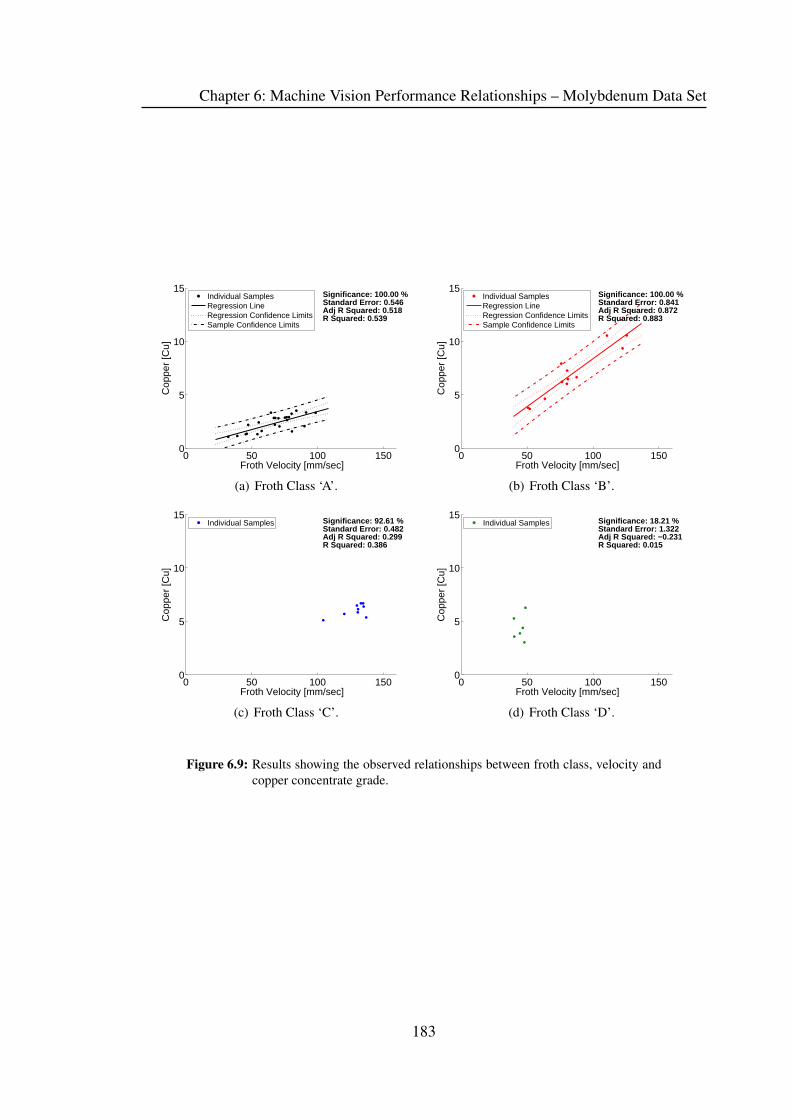
Chapter 6: Machine Vision Performance Relationships – Molybdenum Data Set
0 50 100 1500
5
10
15
Froth Velocity [mm/sec]
Cop
per
[Cu]
R Squared: 0.539Adj R Squared: 0.518Standard Error: 0.546Significance: 100.00 %Individual Samples
Regression LineRegression Confidence LimitsSample Confidence Limits
(a) Froth Class ‘A’.
0 50 100 1500
5
10
15
Froth Velocity [mm/sec]
Cop
per
[Cu]
R Squared: 0.883Adj R Squared: 0.872Standard Error: 0.841Significance: 100.00 %Individual Samples
Regression LineRegression Confidence LimitsSample Confidence Limits
(b) Froth Class ‘B’.
0 50 100 1500
5
10
15
Froth Velocity [mm/sec]
Cop
per
[Cu]
R Squared: 0.386Adj R Squared: 0.299Standard Error: 0.482Significance: 92.61 %Individual Samples
(c) Froth Class ‘C’.
0 50 100 1500
5
10
15
Froth Velocity [mm/sec]
Cop
per
[Cu]
R Squared: 0.015Adj R Squared: −0.231Standard Error: 1.322Significance: 18.21 %Individual Samples
(d) Froth Class ‘D’.
Figure 6.9: Results showing the observed relationships between froth class, velocity and
copper concentrate grade.
183

Chapter 6: Machine Vision Performance Relationships – Molybdenum Data Set
0 50 100 1500
2
4
6
8
10
12
14
Froth Velocity [mm/sec]
Iron
[Fe]
R Squared: 0.492Adj R Squared: 0.469Standard Error: 0.752Significance: 99.99 %Individual Samples
Regression LineRegression Confidence LimitsSample Confidence Limits
(a) Froth Class ‘A’.
0 50 100 1500
2
4
6
8
10
12
14
Froth Velocity [mm/sec]
Iron
[Fe]
R Squared: 0.877Adj R Squared: 0.865Standard Error: 0.716Significance: 100.00 %Individual Samples
Regression LineRegression Confidence LimitsSample Confidence Limits
(b) Froth Class ‘B’.
0 50 100 1500
2
4
6
8
10
12
14
Froth Velocity [mm/sec]
Iron
[Fe]
R Squared: 0.351Adj R Squared: 0.258Standard Error: 0.532Significance: 90.70 %Individual Samples
(c) Froth Class ‘C’.
0 50 100 1500
2
4
6
8
10
12
14
Froth Velocity [mm/sec]
Iron
[Fe]
R Squared: 0.014Adj R Squared: −0.232Standard Error: 1.087Significance: 17.71 %Individual Samples
(d) Froth Class ‘D’.
Figure 6.10: Results showing the observed relationships between froth class, velocity and
iron concentrate grade.
184

Chapter 6: Machine Vision Performance Relationships – Molybdenum Data Set
0 50 100 1500
5
10
15
Froth Velocity [mm/sec]
Mag
nesi
um O
xide
[MgO
]
R Squared: 0.356Adj R Squared: 0.327Standard Error: 1.899Significance: 99.79 %Individual Samples
Regression LineRegression Confidence LimitsSample Confidence Limits
(a) Froth Class ‘A’.
0 50 100 1500
5
10
15
Froth Velocity [mm/sec]
Mag
nesi
um O
xide
[MgO
]
R Squared: 0.874Adj R Squared: 0.861Standard Error: 0.512Significance: 100.00 %Individual Samples
Regression LineRegression Confidence LimitsSample Confidence Limits
(b) Froth Class ‘B’.
0 50 100 1500
5
10
15
Froth Velocity [mm/sec]
Mag
nesi
um O
xide
[MgO
]
R Squared: 0.433Adj R Squared: 0.352Standard Error: 0.658Significance: 94.60 %Individual Samples
(c) Froth Class ‘C’.
0 50 100 1500
5
10
15
Froth Velocity [mm/sec]
Mag
nesi
um O
xide
[MgO
]
R Squared: 0.018Adj R Squared: −0.228Standard Error: 1.256Significance: 19.87 %Individual Samples
(d) Froth Class ‘D’.
Figure 6.11: Results showing the observed relationships between froth class, velocity and
magnesium oxide concentrate grade.
185

Chapter 6: Machine Vision Performance Relationships – Molybdenum Data Set
0 50 100 1500
20
40
60
80
100
120
Froth Velocity [mm/sec]
Mol
ybde
num
Dis
ulfid
e [M
oS2]
R Squared: 0.521Adj R Squared: 0.500Standard Error: 11.780Significance: 99.99 %Individual Samples
Regression LineRegression Confidence LimitsSample Confidence Limits
(a) Froth Class ‘A’.
0 50 100 1500
20
40
60
80
100
120
Froth Velocity [mm/sec]
Mol
ybde
num
Dis
ulfid
e [M
oS2]
R Squared: 0.664Adj R Squared: 0.631Standard Error: 3.382Significance: 99.88 %Individual Samples
Regression LineRegression Confidence LimitsSample Confidence Limits
(b) Froth Class ‘B’.
0 50 100 1500
20
40
60
80
100
120
Froth Velocity [mm/sec]
Mol
ybde
num
Dis
ulfid
e [M
oS2]
R Squared: 0.252Adj R Squared: 0.145Standard Error: 2.373Significance: 83.16 %Individual Samples
(c) Froth Class ‘C’.
0 50 100 1500
20
40
60
80
100
120
Froth Velocity [mm/sec]
Mol
ybde
num
Dis
ulfid
e [M
oS2]
R Squared: 0.014Adj R Squared: −0.232Standard Error: 9.315Significance: 17.71 %Individual Samples
(d) Froth Class ‘D’.
Figure 6.12: Results showing the observed relationships between froth class, velocity and
molybdenum disulphide concentrate grade.
186

Chapter 6: Machine Vision Performance Relationships – Molybdenum Data Set
ferences in the regression models are tested by determining if the models have the same
slope, intercept, and mean value in a statistical sense. If any one of these values is differ-
ent, it means that the regression models are statistically different from one another. The
final column of Table 6.6 is most important, as it shows the confidence in the regression
models being statistically different. It is evident that this is the case for most of the froth
class and assay combinations. These results suggest that the combination of froth velocity
and froth class will account for more of the variation seen in the data than any one of the
measurements alone.
Table 6.6: Summary of the statistical confidence of differences in the froth velocity –
concentrate grade models for the molybdenum data set.
Froth Froth Confidence of Confidence of Confidence of Confidence of
Assay Class Class Difference Difference Difference Difference
1 2 in Slope in Intercept in Mean (Overall)
Copper
A B 100.00 100.00 100.00 100.00A C 6.14 99.95 99.97 99.97A D 4.24 100.00 100.00 100.00B C 94.67 100.00 100.00 100.00B D 33.08 82.96 90.84 90.84
C D 2.20 40.65 69.50 69.50
Iron
A B 3.03 100.00 100.00 100.00A C 25.27 57.23 77.88 77.88
A D 1.60 4.02 51.92 51.92
B C 98.30 100.00 100.00 100.00B D 18.67 99.57 99.75 99.75C D 87.44 100.00 100.00 100.00
Magnesium
A B 4.40 16.43 57.86 57.86
A C 52.32 100.00 100.00 100.00A D 99.97 99.58 99.99 99.99B C 18.37 99.95 99.97 99.97B D 65.10 100.00 100.00 100.00C D 100.00 98.98 99.93 100.00
Molybdenum
A B 1.67 100.00 100.00 100.00A C 10.57 99.40 99.60 99.60A D 99.94 100.00 100.00 100.00B C 9.11 98.32 98.89 98.89B D 90.23 19.67 60.14 90.23
C D 38.91 100.00 100.00 100.00
187

Chapter 6: Machine Vision Performance Relationships – Molybdenum Data Set
The R2, adjusted R2, and standard error values presented in Figures 6.9 to 6.12 are for the
froth class specific regression models. Table 6.7 shows the adjusted R2 values when the
complete model is used to relate froth class, froth velocity, and concentrate grade.
Table 6.7: Adjusted R2 values when froth classes and velocity are used to model the con-
centrate grade of the molybdenum data set.
Cu Fe MgO MoS2
Adjusted R2 0.917 0.899 0.545 0.839
The results show that the combination of froth class and velocity far outperform the use of
either of these measurements on their own to model the concentrate grade. Almost 90%
of the variation in the data can be accounted for in the copper and iron assays, and over
80% of the variation can be accounted for in the molybdenum disulfide assay.
6.6 Feed versus Froth Class
It is possible that the variations seen in the concentrate grade as a function of froth class
are in fact caused by changes in the feed rather than changes in the operation of the cell
being monitored. In order to determine if this the case, it is necessary to determine if
a relationship exists between the feed to the flotation cell and the froth classes that are
identified at the time of sampling.
If no such relationship exists between the froth class and the feed, then one can be sure that
the relationship between the froth velocity, froth class, and concentrate grade presented
in the previous section can be readily used to improve the operation of the flotation cell
being monitored.
However, if there is a relationship between the feed to the flotation cell and the froth class,
it means that it may not be possible to stay in the desired optimal froth class by making
changes to the operating conditions of the flotation cell alone. In such cases, the froth
class information may be used to detect changes in the feed. Personnel can be notified of
such changes and make adjustments to the operating conditions (air flow rate, froth depth,
reagent dosage) which are optimal for the type of feed related to the identified froth class.
188

Chapter 6: Machine Vision Performance Relationships – Molybdenum Data Set
Figure 6.13 shows the observed relationship between the feed to the flotation cell and the
froth classes. Data points to the left hand side of the dotted line are from the left hand
y-axis, and data points to the right hand side of the dotted line correspond to the right hand
y-axis. The data points indicate the mean assay values of the feed for each of the froth
classes (coloured according to the froth classes shown in Figure 6.7). The bars indicate
the range within which 99% of the values fall.
0
5
10
15
20
25
30
35
40
Fee
d A
ssay
Val
ue
0
1
2
3
4
5
6
Cu Fe S SiO2
Al2O
3As MgO MoS
2
Fee
d A
ssay
Val
ueFigure 6.13: Relationship between froth classes and feed to the flotation cell.
From these results, it is evident that the froth class does not give an indication of the feed
to the cell with the exception of froth class ‘D’ (green). Froth class ‘D’ has higher than
normal (froth class ‘A’, ‘B’, ‘C’) copper and aluminium grades. The fact that there is no
major difference between the feeds of the different froth classes indicates that froth class
information can be used to move from one class to another (with the exception of froth
class ‘D’). Plant personnel can therefore make the appropriate adjustments to move to the
desired froth class when the flotation cell is in the ‘A’, ‘B’ or ‘C’ regime. On the other
hand, when froth class ‘D’ is present, the plant personnel will know that this is a result of
a change to the feed in the flotation cell and that different corrective action is required.
189

Chapter 6: Machine Vision Performance Relationships – Molybdenum Data Set
6.7 Process Conditions versus Froth Class
In order to determine how best to operate a flotation cell being monitored by a machine
vision system, it is necessary to determine if there is any relationship between the process
conditions (air flow rate, froth depth, reagent addition, etc.) of the flotation cell and the
machine vision measurements. If such relationships do exist, they can be readily used in
conjunction with the machine vision measurements to optimise the performance of the
flotation cell being monitored.
Figure 6.14 shows the observed relationships between the process conditions of the flota-
tion cell and the froth classes from the molybdenum data set. The data points indicate the
mean values for a given process condition, while the bars indicate the region into which
99% of the measurements fall. Data points to the left of the dotted line should be read off
the left vertical axis and data points to the right of the dotted line should be read off the
right hand vertical axis. The units of the vertical axes are shown in square brackets under
the corresponding measurements on the horizontal axis.
0
100
200
300
400
500
600
0
10
20
30
40
50
Feed Rate[tph]
Frother Dosage[g/m3]
Froth Depth[inches]
pH Percent Solids
Figure 6.14: Relationship between froth classes and process conditions of the flotation
cell.
It is clear that there are considerable differences between the process conditions of the
different froth classes. Class ‘A’ (black) has wide ranges of operation for most of the
190

Chapter 6: Machine Vision Performance Relationships – Molybdenum Data Set
process conditions. This suggests that there is no guaranteed easy way to move the froth
class into this state. The most viable way to achieve a class ‘A’ froth appears to be by
increasing the froth depth of the flotation cell.
Other froth classes (such as class ‘D’ (green)) have much more isolated process condi-
tions. This suggests that by making the appropriate changes to the process conditions the
flotation cell could be made to exhibit a class ‘D’ froth. There are, however, numerous
conditions which could be changed and it is not clear from the limited data presented here
which adjustments should be made to generate a class ‘D’ froth. The results suggest that
a likely way is by decreasing the percent solids to approximately 40% (as this is the only
process condition which has no overlap with the other froth classes).
It is also important to remember that froth class ‘D’ has a higher copper grade in the feed
(see the previous section). This means that it is not yet clear whether it is the percent
solids, the grade of the feed, or a combination of the two which has resulted in froth class
‘D’ being observed. This can only be clarified by performing more test work over a much
longer period.
The results presented in this section have shown that it should be possible to move be-
tween different froth classes by making the appropriate adjustments to the process con-
ditions of the flotation cell. It is not trivial to decouple the effects from the multiple
variables which affect the flotation cells, particularly when a short test work campaign
is performed. Further (long term) work is required to isolate exactly how the different
variables will impact on the observed froth class.
6.8 Summary & Discussion
In this chapter results have been presented for relating machine vision measurements
(froth class and froth velocity) to the concentrate grade of the flotation cell being moni-
tored. These results are summarised in Table 6.8.
For the case where the froth velocity alone is used to model the concentrate grade, re-
sults show that linear models are not appropriate. When a non-linear power model is
fitted to the data, the results are interesting: no additional variation is accounted for, and
the models response is largely linear in the range for which data points were sampled.
191

Chapter 6: Machine Vision Performance Relationships – Molybdenum Data Set
Table 6.8: Summary of standard errors and adjusted R2for predicting copper grade of the
concentrate.
Features Used Copper Iron Magnesium Molybdenum
Froth Velocity (Linear) 0.392 0.589 0.027 0.437
Froth Class 0.684 0.691 0.224 0.676
Froth Class & Velocity 0.917 0.899 0.545 0.839
These results suggest that additional measurements are required to explain the non-linear
variation in the concentrate grade data.
Using bubble size measurements for the molybdenum data set has been shown to be in-
appropriate: it is not always possible to accurately segment the flotation froth images
because the bubbles are sometimes transparent. When this occurs, the assumptions of
the watershed algorithm (and other gradient based bubble delineation algorithms) are vi-
olated, leading to poor segmentations. As an alternative measure to bubble size, texture
measures have been shown to be suitable for identifying different froth classes. Numerous
texture measures have been tested and it has been shown that over 99% correct classifi-
cation can be achieved using Fourier ring based texture measures. Using a linear model,
the texture measures typically account for between 67% and 69% of the variation in the
concentrate grade. This shows that texture measures can be used for the improvement of
the operation of flotation cells.
The combination of froth velocity and froth class information accounts for a much larger
percentage (typically over 20%) of the variation in the data compared to using one of
these parameters to model the concentrate grade of the flotation cell being monitored. For
the copper concentrate grade, over 90% of the variation in the grade can be accounted for
using this simple linear model, while for the iron in the concentrate grade, 89% of the
variation in the data is accounted for.
With the possible exception of froth class ‘D’, the froth classes are not a function of the
feed to the flotation cell. Analysis of the process conditions at the time of operation
suggest that it should be possible to achieve the desired froth class/velocity combination
by making the appropriate adjustments. However, due to the large number of variables
that affect the system it is not clear how best the changes between froth classes are to be
achieved. This is an area where further research is required.
192

Chapter 6: Machine Vision Performance Relationships – Molybdenum Data Set
The combination of an appropriate texture measure, classifier and froth velocity measure
can be used to provide personnel with information related to the concentrate grade of the
cell being monitored. First the class of the current state of the froth is identified. Second,
the froth velocity is measured. The combination of these two measurements can then
be used to give an indication of the current concentrate grade of the cell. Based on this
output value, personnel may either decide to leave the current input variable settings (air
flow rate, froth depth, reagent dosage) or make changes to achieve better performance.
The determination of the optimal froth class and velocity regime to operate in is best made
by experienced metallurgists, as it will typically involve numerous tradeoffs relating to
the concentrate grade of both desirable and undesirable minerals. This should be readily
achievable by analysis of the different froth class/velocity responses (Figures 6.9 to 6.12).
How best to manipulate process conditions to ensure that an optimal froth class is present
on a flotation cell is a difficult problem that requires more research before a set of sys-
tematic approaches can be developed. The results presented here give some indications
of how this may be achieved. However, the limited number of samples, coupled with a
high number of process variables makes it difficult to come to any conclusion with a high
degree of certainty.
While the same concentrate grade can be achieved under different froth class/velocity
regimes, this in no way means that the approach used is inappropriate. While it would be
useful to have the different froth class-velocity responses having no overlap, it is unlikely
that this would be the case: a large number of variables all interact to cause the final
concentrate grade. It is likely that different combinations of the these variables can give
rise to the same concentrate grade. In the same way, it is likely that different combinations
will result in different froth classes being observed, and that at different froth velocities
the same concentrate grade can be achieved.
193

Chapter 6: Machine Vision Performance Relationships – Molybdenum Data Set
194

Chapter 7
Machine Vision PerformanceRelationships – Copper 2006 Data Set
As has been the case for the previous chapters, this chapter addresses objective num-
ber four of the thesis, namely to show that a relationship exists between machine vision
measurements and the metallurgical performance (grade) which can readily be used by
industrial operations. In this chapter, data will be presented from test work carried out
on the copper circuit at Kennecott Utah Copper Concentrator in January 2006. For more
details on the data set, see Section 3.15.
The chapter begins by presenting the observed relationship between froth velocity and
concentrate grade. Next the results of using both linear and non-linear models to relate
the bubble size to concentrate grade are discussed. How bubble size measurements can
be used for the classification of froths with dynamic bubble size distributions, which are
needed to characterise the froths in this data set, are presented next. It is then shown
how unsupervised classification techniques can be used to automatically determine froth
classes based on the bubble size measurements. Next, the relationships between the froth
classes and the concentrate grade of the cell being monitored are presented. This is done
for two reasons, to validate the classes determined automatically, and to show how the
froth class identification can provide useful information about the concentrate grade of the
flotation cell. The combination of froth velocity and froth class for modelling concentrate
grade is then presented.
195

Chapter 7: Machine Vision Performance Relationships – Copper 2006 Data Set
It is important to note that the classification of froth classes in this chapter is entirely
automatic . This is unlike the previous chapters which have presented results which have
been based on an initial hand classification of the flotation froth videos by experienced
personnel. The potential for bias is therefore minimised, and the method is more efficient
for froth class identification.
7.1 Froth Velocity & Concentrate Grade
As mentioned in previous chapters, froth velocity is typically related to the mass flow rate
of the concentrate and to the grade of the concentrate. A simple linear regression model
was fitted to the froth velocity and assay data. The observed relationships between the
froth velocity and concentrate grade of the flotation cell being monitored on the copper
circuit are shown in Figure 7.1.
The observed trends do not account for a large amount of the variation in the data. Only
49% and 64% of the variation in the copper and iron assay data respectively is accounted
for using the froth velocity. Substantially less variation is accounted for in the magnesium
and molybdenum assays.
The observed trends behave as expected. The increase in velocity results in an increased
amount of material non-selectively reporting to the concentrate via entrainment. This
results in an increased amount of gangue being recovered, which decreases the proportion
of floatable material in the concentrate.
Non-linear models of the form
y = a xb + c
were fitted to the data (see Figure 7.2). The result was a lower adjusted R2 value for most
of the assay values (see Table 7.1) due to an increase in the degrees of freedom with no
additional variation in the data being accounted for (an increase of 0.3% was seen in the
adjusted R2 value for the molybdenum disulfide assay). It is also interesting to note that
the non-linear models show a largely linear response, particularly within the bounds of
the observed froth velocities.
196

Chapter 7: Machine Vision Performance Relationships – Copper 2006 Data Set
0 50 100 150 2000
5
10
15
20
25
30
35
40
Cop
per
[Cu]
in C
once
ntra
te
Froth Velocity [mm/sec]
R Squared: 0.495Adj R Squared: 0.490Standard Error: 3.465Significance: 100.00 %Individual Samples
Regression LineRegression Confidence LimitsSample Confidence Limits
0 50 100 150 2000
5
10
15
20
25
30
35
40
45
Iron
[Fe]
in C
once
ntra
te
Froth Velocity [mm/sec]
R Squared: 0.643Adj R Squared: 0.639Standard Error: 2.578Significance: 100.00 %Individual Samples
Regression LineRegression Confidence LimitsSample Confidence Limits
0 50 100 150 2000
1
2
3
4
5
Mag
nesi
um O
xide
[MgO
] in
Con
cent
rate
Froth Velocity [mm/sec]
R Squared: 0.389Adj R Squared: 0.383Standard Error: 0.523Significance: 100.00 %Individual Samples
Regression LineRegression Confidence LimitsSample Confidence Limits
0 50 100 150 2000
1
2
3
4
5
6
7
8
Mol
ybde
num
Dis
ulfid
e [M
oS2] i
n C
once
ntra
te
Froth Velocity [mm/sec]
R Squared: 0.137Adj R Squared: 0.129Standard Error: 1.013Significance: 99.99 %Individual Samples
Regression LineRegression Confidence LimitsSample Confidence Limits
Figure 7.1: Observed linear relationships between froth velocity and concentrate grade.
197

Chapter 7: Machine Vision Performance Relationships – Copper 2006 Data Set
0 50 100 150 2000
5
10
15
20
25
30
35
40
Cop
per
[Cu]
Con
c G
rade
[%]
Froth Velocity [pixels/s]
Individual SamplesRegression LineRegression Confidence LimitsSample Confidence Limits
Significance: 100.00 %Standard Error: 3.499Adj R Squared: 0.485R Squared: 0.495
0 50 100 150 2000
5
10
15
20
25
30
35
40
45
Iron
[Fe]
Con
c G
rade
[%]
Froth Velocity [pixels/s]
Individual SamplesRegression LineRegression Confidence LimitsSample Confidence Limits
Significance: 100.00 %Standard Error: 2.598Adj R Squared: 0.637R Squared: 0.644
0 50 100 150 2000
1
2
3
4
5
Mag
nesi
um O
xide
[MgO
] Con
c G
rade
[%]
Froth Velocity [pixels/s]
Individual SamplesRegression LineRegression Confidence LimitsSample Confidence Limits
Significance: 100.00 %Standard Error: 0.527Adj R Squared: 0.380R Squared: 0.392
0 50 100 150 2000
1
2
3
4
5
6
7
8
Mol
ybde
num
Dis
ulfid
e [M
oS2] C
onc
Gra
de [%
Froth Velocity [pixels/s]
Individual SamplesRegression LineRegression Confidence LimitsSample Confidence Limits
Significance: 99.90 %Standard Error: 1.016Adj R Squared: 0.132R Squared: 0.149
Figure 7.2: Observed non-linear relationships between froth velocity and concentrate
grade.
198

Chapter 7: Machine Vision Performance Relationships – Copper 2006 Data Set
This suggests that the use of froth velocity alone to model the concentrate grade is not suf-
ficient. In order to account for more of the variability in the data it is therefore necessary
to use a combination of froth surface descriptors, rather than froth velocity alone.
Table 7.1: Adjusted R2 values for fitting linear and non-linear models to the relationship
between froth velocity and concentrate grade.
Model Cu Fe MgO MoS2
Linear 0.4903 0.6392 0.3828 0.1287
Non-Linear 0.4853 0.6374 0.3802 0.1318
7.2 Bubble Size & Concentrate Grade
As has been shown in Chapter 4, single value froth descriptors are often inappropriate
to use (especially when the flotation froth exhibits a dynamic bubble size distribution).
For completeness, results are presented here showing the observed relationships between
single value bubble size descriptors and the concentrate grade of the flotation cell for the
copper 2006 data set.
As in Chapter 5, it is still necessary to determine which of the single value descriptors
is most appropriate. Both linear and non-linear power models were fitted to a range of
single value bubble size descriptors. The results from these tests are shown in Table 7.2.
Table 7.2: Average adjusted R2 values for fitting linear and non-linear models to the rela-
tionship between various single value bubble size descriptors and concentrate
grade.
Model Mean p50 p60 p70 p80 p90
Linear 0.1297 0.0550 0.0822 0.1033 0.1240 0.1381Non-Linear 0.1911 0.0793 0.1305 0.1758 0.2153 0.2102
For the linear model the p90 bubble size is best able to account for the variation in the
data, while the p80 bubble size is found to perform the best for the non-linear model. The
resultant linear and non-linear fits when using the p90 and p80 bubble size to model the
concentrate grade for the copper 2006 data set are shown in Figure 7.3 and 7.4.
199

Chapter 7: Machine Vision Performance Relationships – Copper 2006 Data Set
It is evident from the results that the linear models are not well suited to capturing the
relationship between the bubble size and the concentrate grade. Residuals tend to cluster
in groups either above or below the regression line, and it is evident by just observing the
data that a non-linear model is more suited to the task. This is confirmed in Table 7.3,
which presents the adjusted R2 values for the linear and non-linear models and shows that
non-linear models perform better.
Table 7.3: Adjusted R2 values for fitting linear and non-linear models to the relationship
between the p90 bubble size and concentrate grade.
Model Cu Fe MgO MoS2
Linear 0.3554 0.0996 0.0839 0.0136
Non-Linear 0.4239 0.1824 0.1784 0.0765
101
102
103
0
5
10
15
20
25
30
35
40
Cop
per
[Cu]
in C
onc
p90 Bubble Size [pixels2]
Individual SamplesRegression LineRegression Confidence LimitsSample Confidence Limits
Significance: 100.00 %Standard Error: 4.001Adj R Squared: 0.320R Squared: 0.327
Significance: 100.00 %Standard Error: 4.390Adj R Squared: 0.182R Squared: 0.190
Significance: 100.00 %Standard Error: 4.229Adj R Squared: 0.241R Squared: 0.248
Significance: 100.00 %Standard Error: 4.104Adj R Squared: 0.285R Squared: 0.292
Significance: 100.00 %Standard Error: 3.968Adj R Squared: 0.332R Squared: 0.338
Significance: 100.00 %Standard Error: 3.896Adj R Squared: 0.355R Squared: 0.362
101
102
103
0
5
10
15
20
25
30
35
40
45
50
Iron
[Fe]
in C
onc
p90 Bubble Size [pixels2]
Individual SamplesRegression LineRegression Confidence LimitsSample Confidence Limits
Significance: 99.81 %Standard Error: 4.113Adj R Squared: 0.082R Squared: 0.091
Significance: 89.26 %Standard Error: 4.259Adj R Squared: 0.016R Squared: 0.025
Significance: 98.30 %Standard Error: 4.194Adj R Squared: 0.045R Squared: 0.055
Significance: 99.64 %Standard Error: 4.138Adj R Squared: 0.071R Squared: 0.080
Significance: 99.91 %Standard Error: 4.086Adj R Squared: 0.094R Squared: 0.103
Significance: 99.94 %Standard Error: 4.073Adj R Squared: 0.100R Squared: 0.108
101
102
103
0
0.5
1
1.5
2
2.5
3
3.5
4
Mag
nesi
um O
xide
[MgO
] in
Con
c
p90 Bubble Size [pixels2]
Individual SamplesRegression LineRegression Confidence LimitsSample Confidence Limits
Significance: 99.90 %Standard Error: 0.634Adj R Squared: 0.093R Squared: 0.102
Significance: 91.84 %Standard Error: 0.659Adj R Squared: 0.020R Squared: 0.029
Significance: 97.72 %Standard Error: 0.652Adj R Squared: 0.040R Squared: 0.050
Significance: 99.09 %Standard Error: 0.647Adj R Squared: 0.056R Squared: 0.065
Significance: 99.57 %Standard Error: 0.643Adj R Squared: 0.068R Squared: 0.077
Significance: 99.83 %Standard Error: 0.637Adj R Squared: 0.084R Squared: 0.093
101
102
103
0
1
2
3
4
5
6
7
8
9
10
Mol
ybde
num
Dis
ulfid
e [M
oS2] i
n C
onc
p90 Bubble Size [pixels2]
Individual Samples Significance: 93.64 %Standard Error: 1.072Adj R Squared: 0.024R Squared: 0.033
Significance: 74.06 %Standard Error: 1.084Adj R Squared: 0.003R Squared: 0.012
Significance: 72.73 %Standard Error: 1.084Adj R Squared: 0.002R Squared: 0.012
Significance: 71.45 %Standard Error: 1.084Adj R Squared: 0.001R Squared: 0.011
Significance: 73.02 %Standard Error: 1.084Adj R Squared: 0.002R Squared: 0.012
Significance: 87.70 %Standard Error: 1.078Adj R Squared: 0.014R Squared: 0.023
Figure 7.3: Observed linear relationships between p90 bubble size and concentrate grade.
200

Chapter 7: Machine Vision Performance Relationships – Copper 2006 Data Set
101
102
103
0
5
10
15
20
25
30
35
40
Cop
per
[Cu]
in C
onc
p80 Bubble Size [pixels2]
Significance: 100.00 %Standard Error: 3.845Adj R Squared: 0.378R Squared: 0.390
Significance: 100.00 %Standard Error: 4.347Adj R Squared: 0.206R Squared: 0.221
Significance: 100.00 %Standard Error: 4.088Adj R Squared: 0.297R Squared: 0.311
Significance: 100.00 %Standard Error: 3.866Adj R Squared: 0.372R Squared: 0.384
Significance: 100.00 %Standard Error: 3.702Adj R Squared: 0.424R Squared: 0.435
101
102
103
0
5
10
15
20
25
30
35
40
45
50
Iron
[Fe]
in C
onc
p80 Bubble Size [pixels2]
Significance: 99.99 %Standard Error: 3.894Adj R Squared: 0.185R Squared: 0.201
Significance: 70.29 %Standard Error: 4.277Adj R Squared: 0.017R Squared: 0.036
Significance: 96.88 %Standard Error: 4.169Adj R Squared: 0.066R Squared: 0.084
Significance: 99.81 %Standard Error: 4.046Adj R Squared: 0.121R Squared: 0.138
Significance: 99.99 %Standard Error: 3.901Adj R Squared: 0.182R Squared: 0.198
101
102
103
0
0.5
1
1.5
2
2.5
3
3.5
4
Mag
nesi
um O
xide
[MgO
] in
Con
c
p80 Bubble Size [pixels2]
Significance: 100.00 %Standard Error: 0.595Adj R Squared: 0.209R Squared: 0.225
Significance: 91.45 %Standard Error: 0.654Adj R Squared: 0.045R Squared: 0.064
Significance: 99.31 %Standard Error: 0.636Adj R Squared: 0.096R Squared: 0.114
Significance: 99.92 %Standard Error: 0.621Adj R Squared: 0.137R Squared: 0.154
Significance: 99.99 %Standard Error: 0.606Adj R Squared: 0.178R Squared: 0.194
101
102
103
0
1
2
3
4
5
6
7
8
9
10
Mol
ybde
num
Dis
ulfid
e [M
oS2] i
n C
onc
p80 Bubble Size [pixels2]
Significance: 23.00 %Standard Error: 1.095Adj R Squared: −0.008R Squared: 0.011
Significance: 93.04 %Standard Error: 1.063Adj R Squared: 0.050R Squared: 0.068
Significance: 96.17 %Standard Error: 1.056Adj R Squared: 0.062R Squared: 0.080
Significance: 97.81 %Standard Error: 1.050Adj R Squared: 0.073R Squared: 0.091
Significance: 98.12 %Standard Error: 1.048Adj R Squared: 0.077R Squared: 0.094
Figure 7.4: Observed non-linear power relationships between p90 bubble size and con-
centrate grade.
201

Chapter 7: Machine Vision Performance Relationships – Copper 2006 Data Set
7.3 Automatic Classification of Froth Classes using Bub-ble Size Distributions
In Section 4.3, an algorithm was presented which can automatically detect froth classes
from bubble size distribution data by first characterising the froths according to their bub-
ble size distribution dynamics, and then using an unsupervised clustering algorithm to
cluster the characterised froths into froth classes.
This same method is used here to automatically cluster the data from the copper 2006
data set into froth classes. Unlike the example in Section 4.3, a slightly modified ver-
sion, which allows some user intervention, is presented here. The first step in the learning
process is to identify the bubble size distributions which occur frequently throughout the
entire data set. The froth video sequences are sampled to get a representative sample of
froth images. The bubble size distribution is then calculated for each of these images,
and the bubble size distributions are presented to an unsupervised classification algorithm
(see Section 3.8.2 for details on unsupervised classification). The results from the un-
supervised classification algorithm are shown in Figure 7.5. Figure 7.6 shows example
images of froths with the bubble size distributions shown in Figure 7.5.
At this stage it is possible to characterise video clips of froth as histograms of frequently
occurring bubble size distributions. These characteristic histograms are passed to an un-
supervised clustering algorithm to determine the nine most frequently occurring charac-
teristic histograms. Figure 7.7 shows the resulting nine most frequently occurring charac-
teristic histograms from the copper 2006 data set.
Although one could in principle use the nine output froth classes to determine the links
between froth class and metallurgy for the data set, having such a high number of froth
classes will result in statistically insignificant models relating the froth classes and con-
centrate grade. This is because of the limited number of metallurgical samples in the data
set.
Visual inspection of the characteristic histograms reveals that many are similar to one an-
other (for example Figure 7.7b and 7.7c). From this set of characteristic clusters a subset
of clusters is chosen. This is done in a similar manner to the classification of other froth
data sets by hand. An experienced operator can gauge how visually similar the froths are
202

Chapter 7: Machine Vision Performance Relationships – Copper 2006 Data Set
100
101
102
103
104
0
20
40
60
80
100
Bubble Size [pixels2]
Per
cent
age
Pas
sing
ABCDEFGH
Figure 7.5: Frequently occurring BSDs learnt from 9000 samples.
Figure 7.6: Example images of the froths represented by the cumulative BSDs in Fig-
ure 7.5.
203

Chapter 7: Machine Vision Performance Relationships – Copper 2006 Data Set
A B C D E F G H0
10
20
30
40
50
60
Per
cent
age
of T
ime
Larger Bubbles Smaller Bubbles
(a)
A B C D E F G H0
10
20
30
40
50
60
Per
cent
age
of T
ime
Larger Bubbles Smaller Bubbles
(b)
A B C D E F G H0
10
20
30
40
50
60
Per
cent
age
of T
ime
Larger Bubbles Smaller Bubbles
(c)
A B C D E F G H0
10
20
30
40
50
60
Per
cent
age
of T
ime
Larger Bubbles Smaller Bubbles
(d)
A B C D E F G H0
10
20
30
40
50
60
Per
cent
age
of T
ime
Larger Bubbles Smaller Bubbles
(e)
A B C D E F G H0
10
20
30
40
50
60
Per
cent
age
of T
ime
Larger Bubbles Smaller Bubbles
(f)
A B C D E F G H0
10
20
30
40
50
60
Per
cent
age
of T
ime
Larger Bubbles Smaller Bubbles
(g)
A B C D E F G H0
10
20
30
40
50
60
Per
cent
age
of T
ime
Larger Bubbles Smaller Bubbles
(h)
A B C D E F G H0
10
20
30
40
50
60
Per
cent
age
of T
ime
Larger Bubbles Smaller Bubbles
(i)
Figure 7.7: Nine detected characteristic histograms of the copper 2006 data set.
204

Chapter 7: Machine Vision Performance Relationships – Copper 2006 Data Set
using the nine characteristic histograms as indicators. From the set of histograms, three
are chosen which best represent the original set of nine. The result is that the characteristic
histograms of Figure 7.7b, 7.7e and 7.7h are chosen as froth classes.
The reason for choosing these specific characteristic histograms is that there are only
a small number of video segments that can be characterised by the histograms in Fig-
ures 7.7a and 7.7i; they are therefore not representative of the data set as a whole. Fur-
thermore, the remaining characteristic histograms have many similarities: the selection of
characteristic histograms b,e and h results in the most representative set of characteristic
histograms for the copper data set.
The individual froth video segments from the data set can now be classified according to
which of these three characteristic histograms they are most similar to. The final set of
characteristic histograms is shown in Figure 7.8. Appendix F contains the characteristic
histograms for each of the samples in the 2006 copper data set.
205

Chapter 7: Machine Vision Performance Relationships – Copper 2006 Data Set
A B C D E F G H0
10
20
30
40
50
60
Per
cent
age
of T
ime
Larger Bubbles Smaller Bubbles
(a) Froth Class ‘A’.
A B C D E F G H0
10
20
30
40
50
60
Per
cent
age
of T
ime
Larger Bubbles Smaller Bubbles
(b) Froth Class ‘B’.
A B C D E F G H0
10
20
30
40
50
60
Per
cent
age
of T
ime
Larger Bubbles Smaller Bubbles
(c) Froth Class ‘C’.
Figure 7.8: Final set of three froth class characteristic histograms.
206

Chapter 7: Machine Vision Performance Relationships – Copper 2006 Data Set
7.4 Froth Class & Concentrate Grade
Once the flotation images has been classified into froth classes, the class information can
be used as a parameter in modelling concentrate grade. Figure 7.9 shows the observed
relationships between the froth classes and the concentrate grade of the flotation cell being
monitored, while Table 7.4 summarises the adjusted R2 values when froth classes are used
to model the concentrate grade.
The results presented in Figure 7.9 may not appear to be particularly useful, because of
the large degree of overlap between the data from the different froth classes. However,
this is not as big a problem as one might initially expect. It is important to remember
that the mean assay values for the different froth classes and the associated standard error
values are crucial for the correct interpretation of the data. Table 7.5 shows the mean
assay values and standard deviations for the different froth classes identified.
If the mean values of the different froth classes are significantly different from one an-
other, then the froth class information is very useful for the operation of the flotation cell
being monitored. This is the case for the data presented here. Table 7.6 clearly shows
that there is a statistically significant difference in the mean values for the different froth
classes for most of the assay values (values which have significance of over 95% are high-
lighted). This means that it is more beneficial to operate in a froth ‘class C’ than in a ‘class
A’ regime. The benefits are a 70% increase in copper grade and a 26% decrease in the
magnesium oxide grade.
While the results show that there is long term benefit to operating under specific froth
class regimes, the results also show that the froth class information alone is not sufficient
to account for most of the variation seen in the concentrate assay values. The linear model
based of the froth classes alone is able to account for 46% of the variation in the copper
data and only for 26% and 24% of the variation seen in the iron and magnesium oxide
data respectively. Therefore in order to explain more of the variation in the data, and in so
doing to be able to achieve better prediction when the model is used, the use of additional
machine vision surface descriptors in the model is required.
207

Chapter 7: Machine Vision Performance Relationships – Copper 2006 Data Set
A B C0
5
10
15
20
25
30
35
Froth Class
Cop
per
[Cu]
Std Err: 3.575R2: 0.473Adj R2: 0.457
A B C0
5
10
15
20
25
30
35
Froth Class
Iron
[Fe]
Std Err: 3.701R2: 0.278Adj R2: 0.256
A B C0
0.5
1
1.5
2
2.5
3
3.5
4
4.5
5
Froth Class
Mag
nesi
um O
xide
[MgO
]
Std Err: 0.580R2: 0.264Adj R2: 0.242
A B C0
1
2
3
4
5
6
7
8
Froth Class
Mol
ybde
num
Dis
ulfid
e [M
oS2]
Std Err: 1.053R2: 0.087Adj R2: 0.059
Figure 7.9: Observed relationships between froth class and concentrate grade.
208

Chapter 7: Machine Vision Performance Relationships – Copper 2006 Data Set
Table 7.4: Adjusted R2 values when froth classes are used to model the concentrate grade.
Cu Fe MgO MoS2
Adjusted R2 0.4572 0.2565 0.2423 0.0592
Table 7.5: Mean values of the concentrate grade for the copper froth classes.
Froth ClassCopper Iron Magnesium Molybdenum
Mean Std Dev Mean Std Dev Mean Std Dev Mean Std Dev
A 12.99 4.04 20.39 4.40 2.01 0.73 2.13 1.24
B 19.68 3.28 25.66 3.27 1.21 0.50 2.82 1.07
C 22.09 3.67 23.74 3.78 1.48 0.54 2.27 0.39
Table 7.6: Summary of the statistical confidence of differences in the mean value of the
concentrate for various mineral and froth class combinations using Welch’s
t-test.
Class 1 Class 2 Copper Iron Magnesium Molybdenum
A B 100.0 100.0 100.0 98.5A C 100.0 99.0 99.2 40.7
B C 97.8 93.1 92.6 99.8
209

Chapter 7: Machine Vision Performance Relationships – Copper 2006 Data Set
7.5 Froth Class, Velocity & Concentrate Grade
As seen in previous chapters, the combination of froth velocity and froth class measure-
ments have resulted in improved models of the concentrate grade. This section presents
the results of using the combination of froth class and froth velocity to model the concen-
trate grade assays of the copper 2006 data set.
A model of the form
y = β0 + β1X + γ1C1 + γ2C2 + ε
is used to relate the froth class and froth velocity to the concentrate grade data, where
βi and γi are the regression coefficients, and Ci are indicator variables that represent the
froth classes, X is the froth velocity, and ε is the residual error in the model [10].
The results showing the observed relationships are shown in Figures 7.10 to 7.13. It is
evident that a combination of froth class and linear relationship between froth velocity and
concentrate is well suited for modelling the relationship between froth class, velocity, and
concentrate grade. It is also important to note that the adjusted R2 parameters are given
for the linear model relating froth velocity to concentrate grade on a ‘per froth class’ basis.
The actual adjusted R2 values for the entire model are given in Table 7.7. The model is
able to account for over 65% of the variation in the concentrate grade data for both the
copper and the iron assays.
Table 7.7: Adjusted R2 values when froth classes and velocity are used to model the con-
centrate grade.
Cu Fe MgO MoS2
Adjusted R2 0.6758 0.6564 0.4411 0.1323
It is important to note that for each of the assays in Figures 7.10 to 7.13, the observed
regression lines relating froth velocity to concentrate grade for the different froth classes
have different slopes and centres of mass. These results prove that the unsupervised clas-
sification algorithm used in Section 7.3 are real froth classes and not just random allo-
cations. If the froth classes had been random, there would be no statistical differences
between the observed trends. Table 7.8 shows the results from the statistical analysis to
determine whether the observed trends have statistically different regression lines. The
210

Chapter 7: Machine Vision Performance Relationships – Copper 2006 Data Set
0 50 100 150 2000
10
20
30
40
Froth Velocity [mm/sec]
Cop
per
[Cu]
R Squared: 0.302Adj R Squared: 0.275Standard Error: 3.438Significance: 99.76 %Individual Samples
Regression LineRegression Confidence LimitsSample Confidence Limits
(a) Froth Class ‘A’.
0 50 100 150 2000
10
20
30
40
Froth Velocity [mm/sec]
Cop
per
[Cu]
R Squared: 0.395Adj R Squared: 0.385Standard Error: 2.569Significance: 100.00 %Individual Samples
Regression LineRegression Confidence LimitsSample Confidence Limits
(b) Froth Class ‘B’.
0 50 100 150 2000
10
20
30
40
Froth Velocity [mm/sec]
Cop
per
[Cu]
R Squared: 0.629Adj R Squared: 0.605Standard Error: 2.309Significance: 99.99 %Individual Samples
Regression LineRegression Confidence LimitsSample Confidence Limits
(c) Froth Class ‘C’.
Figure 7.10: Observed relationships between froth velocity, froth class and concentrate
grade.
211

Chapter 7: Machine Vision Performance Relationships – Copper 2006 Data Set
0 50 100 150 2000
10
20
30
40
Froth Velocity [mm/sec]
Iron
[Fe]
R Squared: 0.592Adj R Squared: 0.577Standard Error: 2.859Significance: 100.00 %Individual Samples
Regression LineRegression Confidence LimitsSample Confidence Limits
(a) Froth Class ‘A’.
0 50 100 150 2000
10
20
30
40
Froth Velocity [mm/sec]
Iron
[Fe]
R Squared: 0.431Adj R Squared: 0.421Standard Error: 2.489Significance: 100.00 %Individual Samples
Regression LineRegression Confidence LimitsSample Confidence Limits
(b) Froth Class ‘B’.
0 50 100 150 2000
10
20
30
40
Froth Velocity [mm/sec]
Iron
[Fe]
R Squared: 0.704Adj R Squared: 0.684Standard Error: 2.122Significance: 100.00 %Individual Samples
Regression LineRegression Confidence LimitsSample Confidence Limits
(c) Froth Class ‘C’.
Figure 7.11: Observed relationships between froth velocity, froth class and concentrate
grade.
212

Chapter 7: Machine Vision Performance Relationships – Copper 2006 Data Set
0 50 100 150 2000
1
2
3
4
5
Froth Velocity [mm/sec]
Mag
nesi
um O
xide
[MgO
]
R Squared: 0.172Adj R Squared: 0.140Standard Error: 0.680Significance: 97.18 %Individual Samples
Regression LineRegression Confidence LimitsSample Confidence Limits
(a) Froth Class ‘A’.
0 50 100 150 2000
1
2
3
4
5
Froth Velocity [mm/sec]
Mag
nesi
um O
xide
[MgO
]
R Squared: 0.181Adj R Squared: 0.166Standard Error: 0.456Significance: 99.92 %Individual Samples
Regression LineRegression Confidence LimitsSample Confidence Limits
(b) Froth Class ‘B’.
0 50 100 150 2000
1
2
3
4
5
Froth Velocity [mm/sec]
Mag
nesi
um O
xide
[MgO
]
R Squared: 0.804Adj R Squared: 0.790Standard Error: 0.245Significance: 100.00 %Individual Samples
Regression LineRegression Confidence LimitsSample Confidence Limits
(c) Froth Class ‘C’.
Figure 7.12: Observed relationships between froth velocity, froth class and concentrate
grade.
213

Chapter 7: Machine Vision Performance Relationships – Copper 2006 Data Set
0 50 100 150 2000
1
2
3
4
5
6
Froth Velocity [mm/sec]
Mol
ybde
num
Dis
ulfid
e [M
oS2]
R Squared: 0.122Adj R Squared: 0.088Standard Error: 1.183Significance: 93.14 %Individual Samples
(a) Froth Class ‘A’.
0 50 100 150 2000
1
2
3
4
5
6
Froth Velocity [mm/sec]
Mol
ybde
num
Dis
ulfid
e [M
oS2]
R Squared: 0.039Adj R Squared: 0.022Standard Error: 1.063Significance: 86.68 %Individual Samples
(b) Froth Class ‘B’.
0 50 100 150 2000
1
2
3
4
5
6
Froth Velocity [mm/sec]
Mol
ybde
num
Dis
ulfid
e [M
oS2]
R Squared: 0.394Adj R Squared: 0.353Standard Error: 0.311Significance: 99.30 %Individual Samples
Regression LineRegression Confidence LimitsSample Confidence Limits
(c) Froth Class ‘C’.
Figure 7.13: Observed relationships between froth velocity, froth class and concentrate
grade.
214

Chapter 7: Machine Vision Performance Relationships – Copper 2006 Data Set
results show that, in the case of copper grade, the model of combined parameters is statis-
tically significant, with over 65% of the variation in the data being explained by the model.
This indicates that froth class and froth velocity are a particular successful combination
when modelling concentrate grade for the copper 2006 data set.
Table 7.8: Summary of the statistical confidence of differences in the froth velocity - con-
centrate grade models for the copper 2006 data set.
Froth Froth Confidence of Confidence of Confidence of Confidence of
Assay Class Class Difference Difference Difference Difference
A B in Slope in Intercept in Mean (Overall)
Copper
1 2 63.07 99.99 100.00 100.001 3 95.30 100.00 100.00 100.002 3 94.58 100.00 100.00 100.00
Iron
1 2 37.97 90.30 95.08 95.081 3 93.21 9.60 54.94 93.21
2 3 97.73 57.88 79.62 97.73
Magnesium
1 2 2.26 99.27 99.62 99.621 3 95.51 65.00 83.39 95.512 3 99.34 66.07 84.10 99.34
Molybdenum
1 2 34.41 53.53 76.66 76.66
1 3 2.23 53.10 76.28 76.28
2 3 23.99 87.99 93.88 93.88
7.6 Feed versus Froth Class
As in the previous chapters, the effect of the flotation feed grade on the froth surface
descriptors needs to be examined. It is useful to determine if a relationship exists between
the feed to the flotation cell being observed and the froth classes observed. If there is a
relationship, then it is possible that the froth class is driven by the feed to the flotation cell,
rather than by the process parameters under which the flotation cell is being operated. If
this is the case, then the machine vision system can be used to alert plant personnel when
changes in the feed to the flotation cell (indicated by a change in froth class) has occurred.
The necessary steps can then be made to adjust the process parameters of the flotation cell
to ensure that optimal performance is achieved.
215

Chapter 7: Machine Vision Performance Relationships – Copper 2006 Data Set
Figure 7.14 shows the observed relationship between the feed to the flotation cell and the
froth classes. Data points to the left hand side of the dotted line are from the left hand
y-axis, and data points to the right hand side of the dotted line correspond to the right
hand y-axis. The data points indicate the mean assay values of the feed for each of the
froth classes. The bars indicate the range within which 99% of the values fall.
0
10
20
30
40
50
60
Fee
d A
ssay
Val
ue
0
0.5
1
1.5
2
2.5
Al2O
3Fe MgO SiO
2Cu MoS
2S
Fee
d A
ssay
Val
ue
Figure 7.14: Relationship between froth classes and feed to the flotation cell.
Figure 7.15 shows the observed relationship between the p80 bubble size and the feed to
the flotation cell being monitored.
It is evident from the results that there is no clear relationship between the feed to the
flotation cell and the bubble size or froth class identified. These results also suggest that
it will be possible for operators to move between froth classes by making the appropriate
adjustments as the froth classes are not determined by the feed to the cell.
7.7 Process Conditions versus Froth Class
Figure 7.16 shows the relationships between the froth classes and the process parameters
at the times when the froth classes were present. Data points to the left hand side of the
216

Chapter 7: Machine Vision Performance Relationships – Copper 2006 Data Set
101
102
103
5.5
6
6.5
7
Alu
min
ium
Oxi
de [A
l 2O3]
p80 Bubble Size [pixels2]10
110
210
30.35
0.4
0.45
0.5
0.55
0.6
0.65
0.7
0.75
Cop
per
[Cu]
p80 Bubble Size [pixels2]
101
102
103
2.5
3
3.5
4
4.5
5
Iron
[Fe]
p80 Bubble Size [pixels2]10
110
210
32
2.5
3
3.5
4
4.5
5
Mag
nesi
um O
xide
[MgO
]
p80 Bubble Size [pixels2]
101
102
103
0.06
0.07
0.08
0.09
0.1
0.11
0.12
0.13
Mol
ybde
num
Dis
ulfid
e [M
oS2]
p80 Bubble Size [pixels2]10
110
210
30.4
0.6
0.8
1
1.2
1.4
1.6
1.8
2
Sul
phur
[S]
p80 Bubble Size [pixels2]
Figure 7.15: Relationships between p80 bubble size and feed grade for the copper 2006
data set.
217
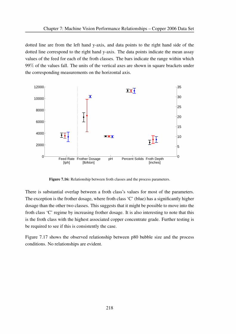
Chapter 7: Machine Vision Performance Relationships – Copper 2006 Data Set
dotted line are from the left hand y-axis, and data points to the right hand side of the
dotted line correspond to the right hand y-axis. The data points indicate the mean assay
values of the feed for each of the froth classes. The bars indicate the range within which
99% of the values fall. The units of the vertical axes are shown in square brackets under
the corresponding measurements on the horizontal axis.
0
2000
4000
6000
8000
10000
12000
0
5
10
15
20
25
30
35
Feed Rate[tph]
Frother Dosage[lb/kton]
pH Percent Solids Froth Depth[inches]
Figure 7.16: Relationship between froth classes and the process parameters.
There is substantial overlap between a froth class’s values for most of the parameters.
The exception is the frother dosage, where froth class ‘C’ (blue) has a significantly higher
dosage than the other two classes. This suggests that it might be possible to move into the
froth class ‘C’ regime by increasing frother dosage. It is also interesting to note that this
is the froth class with the highest associated copper concentrate grade. Further testing is
be required to see if this is consistently the case.
Figure 7.17 shows the observed relationship between p80 bubble size and the process
conditions. No relationships are evident.
218

Chapter 7: Machine Vision Performance Relationships – Copper 2006 Data Set
101
102
103
2800
3000
3200
3400
3600
3800
4000
4200
4400
Fee
d R
ate
[tph]
p80 Bubble Size [pixels2]10
110
210
332
32.5
33
33.5
34
34.5
Per
cent
Sol
ids
p80 Bubble Size [pixels2]
101
102
103
5
6
7
8
9
10
11
12
Fro
th D
epth
[inc
hes]
p80 Bubble Size [pixels2]10
110
210
39.4
9.6
9.8
10
10.2
10.4
10.6
10.8
11
pH
p80 Bubble Size [pixels2]
101
102
103
14
16
18
20
22
24
26
28
30
32
Fro
ther
Dos
age
[lb/k
ton]
p80 Bubble Size [pixels2]
Figure 7.17: Relationships between p80 bubble size and process conditions for the copper
2006 data set.
219

Chapter 7: Machine Vision Performance Relationships – Copper 2006 Data Set
7.8 Summary & Discussion
The results presented in this chapter have shown that relationships exist between:
• froth velocity and concentrate grade
• froth bubble size and concentrate grade
• froth class and concentrate grade.
Results have shown that when froth velocity is used to model the concentrate grade, a
linear model is sufficient. Results from using a non-linear model do not account for
more variation in the data than the linear model. Furthermore, the best fit non-linear
models tend to have largely linear responses in the ranges where the velocity values were
sampled.
For the single value bubble size measurements, a non-linear relationship exists between
the measurement and the concentrate grade values. The use of non-linear models is more
appropriate as they fit the data better, accounting for more variation in the data. The use
of multiple non-linear models to relate the froth velocity and bubble size measurements
to concentrate grade are beyond the scope of this thesis, and have not been presented.
Techniques for automatically detecting and characterising froth classes from flotation
froths which exhibit dynamic bubble size distributions have been presented. The result-
ing froth classes have been validated by showing that the relationship between the froth
velocity and concentrate grade is statistically significantly different for each of the froth
classes, something which would not occur had the classes been the result of a random
class allocation. This technique allows for the consistent identification of froth classes
in a simple time efficient manner. Classifying froth classes by hand is a time consuming
task and is particularly difficult when the froths being classified have dynamic bubble size
distributions.
The relationship between the froth classes and the concentrate grade has been shown to
account for a greater percentage of the variation seen in the concentrate grade data than
using single value bubble size descriptors when both linear and non-linear models are
used (see Table 7.9).
220

Chapter 7: Machine Vision Performance Relationships – Copper 2006 Data Set
The best results are obtained when a combination of froth class and froth velocity are
used to model the concentrate grade. Such models account for over 65% of the variation
seen in the copper and iron concentrate grade. The results also show that the relationship
between froth velocity and concentrate grade is different for each of the froth classes. This
effect provides valuable insight for plant personnel on how to achieve better performance
of the flotation cell being monitored. Under a certain froth class regime, they will be able
to adjust the velocity of the froth so that the desired grade set point can be achieved.
The results from this chapter are summarised in Table 7.9, which shows the adjusted R2
values for each of the variables used to model the concentrate grade of the copper 2006
data set.
Table 7.9: Adjusted R2 values for fitting various models to concentrate grade.
Model Cu Fe MgO MoS2
Froth Velocity (Linear) 0.4903 0.6392 0.3828 0.1287
Froth Velocity (Non-Linear) 0.4853 0.6374 0.3802 0.1318
Bubble Size (Linear) 0.3554 0.0996 0.0839 0.0136
Bubble Size (Non-Linear) 0.4239 0.1824 0.1784 0.0765
Froth Class 0.4572 0.2565 0.2423 0.0592
Froth Class & Velocity 0.6758 0.6564 0.4411 0.1323
Analysis of the feed to the flotation cell at the time of sampling has shown that there is
no significant relationship between the feed assay results and the froth class present or
the bubble size of the flotation froth. This means that machine vision systems will not be
suited to detecting changes in the feed to the flotation cell. It is important to remember,
that the data presented here is the assay values of the feed. These do not completely
describe the feed to the cell. Further research looking at the assays on a size by size and
mineralogical basis could reveal that there is a relationship between these aspects of the
feed to the flotation cell and the froth class observed on the surface. If this is the case,
the froth class identification can also be used to alert the plant personnel to changing feed
conditions and the appropriate corrective action can then be taken.
Analysis of the process conditions at the time of sampling has revealed that froth class
‘C’ occurred when the frother dosage was relatively high. What is interesting to note is
that this observation is not clear in Figure 7.17, which shows the relationship between the
p80 bubble size and the various process conditions. This once again highlights one of the
221

Chapter 7: Machine Vision Performance Relationships – Copper 2006 Data Set
advantages of using froth classes instead of single value descriptors to characterise the
bubble size distribution of a flotation froth.
As has already been seen for the molybdenum data set, the metallurgical results for the
copper 2006 data set also show how the identification of froth classes and measurement of
froth velocity can provide plant personnel with valuable information pertaining to the con-
centrate grade of the flotation cell being monitored. It has been shown that it is possible to
identify which froth class has the best metallurgical performance (in terms of concentrate
grade of the desired metal). The machine vision system can be used to identify whether
the flotation cell is operating under the desired conditions or not. In this manner, personnel
can be alerted to undesirable operational conditions and make the necessary adjustments
to improve the performance of the flotation cell.
As has been mention in the discussion section of the previous chapter (Section 6.8), the
fact that different froth class/velocity combinations can give rise to the same concentrate
grade is not unexpected. In fact, it can be of direct benefit to the plant personnel. This
means that there is often a choice of how they can move to the desired concentrate grade
set point. For example, if it is not known how to change between different froth classes,
the froth velocity may be adjusted to achieve the desired results.
222

Chapter 8
Summary, Conclusions & Further Work
8.1 Summary
The review of the literature on machine vision systems for analysing flotation froths has
revealed a number of items which still need to be addressed before machine vision systems
become a standard feature in froth flotation operations.
8.1.1 Improved Bubble Size Measurement
Until now, the current state of the art bubble size measurement algorithms have been lim-
ited to providing accurate bubble size measurements on flotation froths with homogenous
bubble size distributions only. Analysis of flotation froths with both large and tiny bubbles
present has resulted in poor segmentation results.
An improvement to the watershed algorithm has been developed which enables the ac-
curate determination of froth bubble size distributions when both large and tiny bubbles
are present simultaneously. The new algorithm makes use of a texture based classifier
to determine whether the output blobs from a single pass watershed algorithm have been
successfully identified, or if they are in fact a collection of tiny bubbles which requires
further segmentation. The classifier uses a simple threshold on the contrast feature, de-
223

Chapter 8: Summary, Conclusions & Further Work
termined from a greyscale co-occurrence matrix. The classification stage’s output is used
to modify the input image such that a second pass of the watershed algorithm can be
performed using different parameters optimised for smaller bubble detection. The modi-
fications to the input image are such that the second stage of watershed processing retains
the correct segmentation from the large bubbles as identified by the first watershed stage.
It is possible to adjust the algorithm so that it has as many stages as desired. Experi-
mentation shows that more than three levels are not useful for images 320×240 pixels in
size.
8.1.2 Characterisation of Froths with Dynamic BSDs
The most effective way to deal with the abundance of information that is present in ac-
curate bubble size distributions has been an important but unexplored area of research.
Typically bubble size distributions are reduced to a single value descriptor such as a mean
or p80 value. Such simplifications of bubble size distribution data are often inappropri-
ate, as too much information is lost. This results in the inability to differentiate between
froths with different bubble size distributions. This is a particular problem for flotation
froths which exhibit dynamic bubble size distributions. For these froths it is imperative
that appropriate data reduction techniques are used. A number of methods for charac-
terising flotation froths with dynamic bubble size distributions have been proposed and
tested. The best of these is the characterisation of flotation froths with a histogram of
their frequently occurring bubble size distributions.
An extension to the characterisation of flotation froths using a histogram of frequently
occurring bubble size distributions has also been presented. In this extension, an unsuper-
vised classification algorithm is used to automatically learn the froth classes from a data
set of flotation froths which exhibit dynamic bubble size distributions. The results of the
algorithm are shown to be true froth classes rather than a random assignment of samples
to froth classes. This is achieved by showing that the relationship between froth velocity
and concentrate grade is statistically different for each of the froth classes.
224

Chapter 8: Summary, Conclusions & Further Work
8.1.3 Texture Measures for Flotation Froths
Previous researchers have used a number of different texture measures for the classifica-
tion of flotation froth images. However, most of the researchers give no reasons for their
choice of texture measure. This problem is compounded by the fact that most researchers
use data sets a single industrial operation. There are also no freely available databases of
flotation froths on which the variety of texture measures can be tested in order to deter-
mine their efficiency.
A large number of texture measures were tested on a data set that consists of a variety
of flotation froths from a number of different industrial operations. The data set consists
of 18 different froth classes, with a total of 16793 images. The results showed that most
texture measures perform well at discriminating between different froths. Laws’ filter
masks and Gabor filters showed the best results. However, implementation of these tex-
ture features is not always advisable, as their improved performance comes at a cost of
increased processing time. Texture measures based on Fourier rings and texture spectrum
have shown to provide good results while maintaining a simple implementation and the
quick classification of new samples.
8.1.4 Surface Descriptor - Concentrate Grade Relationships
The advanced methodology developed to measure the bubble size and texture of flotation
froths was used to determine the existence of relationships between froth surface descrip-
tors and the concentrate grade of the cell being monitored. Data sets from three different
industrial operations were used to show how machine vision systems can be used when
different types of froth are present.
8.1.4.1 Platinum Data Set
The relationship between froth velocity and concentrate grade was examined. The results
showed that a non-linear power model accounted for more of the variation in the data than
a linear model.
225

Chapter 8: Summary, Conclusions & Further Work
Analysis of the relationship between single value bubble size measurements and the con-
centrate grade showed that the mean bubble size measurement performed best when linear
models were used and that the p80 measurement performed best when non-linear power
models were used. The results showed that non-linear power models were better suited
to model the concentrate grade, as they explained on average 7% more of the variation in
the data than a linear model.
Analysis of the relationship between the froth classes and the concentrate grade showed
that on average 69% of the variation in the data could be accounted for using froth class
information alone.
The results from tests combining the froth velocity, bubble size and froth class informa-
tion to better explain the variation in the concentrate grade were inconclusive. The results
did not improve the amount of variation in the data that could be explained. There are
two reasons for this result. Firstly, there was not sufficient froth velocity range associated
with each of the froth classes to result in an improved relationships. Secondly, the bub-
ble size and froth velocity measurements were co-linear. This resulted in no significant
improvement when the combination of froth velocity and bubble size were used to model
the concentrate grade.
Examination of the various methods tested showed that the best model fit for the concen-
trate grade could be achieved using one of: froth velocity, froth class, and bubble size
measurements. Froth velocity gave best results for PGM and copper assays, froth class
the best results for the nickel, sulfur and chromite assays, and bubble size measures gave
the best results for the iron assay.
8.1.4.2 Molybdenum Data Set
In the second industrial case study, texture measurements were used to identify froth
classes of a flotation froth for which accurate bubble size measurements were not possible,
because of transparent bubbles. The concentrate grade was modelled as a function of froth
velocity, froth class and the combination of froth velocity and class.
The concentrate grade was modelled as a function of the froth velocity using both linear
and non-linear models. The results showed that neither model was particularly well suited
226

Chapter 8: Summary, Conclusions & Further Work
to explaining the data. The non-linear model was found to have a largely linear response
for the range of froth velocities sampled. The linear model was found to account for an
average of 36% of the variation in the data, while the non-linear model accounted for an
average of 38% of the variation in the concentrate grade data.
When the concentrate grade was modelled using a linear function of froth class, an av-
erage of 57% of the variation in the data could be accounted for. The addition of froth
velocity to the model, resulted in a further improvement. When the combination of froth
velocity and froth class were used to model the concentrate grade, an average of 80% of
the variation in the concentrate assay data could be accounted for.
Analysis of the feed to the flotation cell at the time of sampling indicates that for one
of the froth classes present there is a statistically significantly higher copper feed grade.
This suggests that froth class information can be used to provide information pertaining
to the feed to the flotation cell. Analysis of the process conditions at the time of sampling
suggests that it may be possible to move between the different froth classes by changing
process conditions. However, due to the high dimensionality of the variables which can
result in the presence of a specific froth class, it is not possible to know if the feed or the
process conditions were the dominant factor that caused a particular froth class. Further
investigations are required to this end.
8.1.4.3 Copper 2006 Data Set
In the final case study, froth class identification is achieved automatically using an un-
supervised clustering algorithm. This is necessary as the flotation froth in this data set
exhibits a dynamic bubble size distribution. However, for the sake of completeness, the
relationship between single value bubble size descriptors and the concentrate grade have
been analysed as well.
As was the case for the molybdenum and platinum data sets, both linear and non-linear
models were used to relate the froth velocity to the concentrate grade. Again, there was
minimal difference between the two models, with the non-linear model having a largely
linear response for the ranges of froth velocity sampled. An average of 41% of the varia-
tion in the copper data could be accounted for using froth velocity alone.
227

Chapter 8: Summary, Conclusions & Further Work
As was the case for the platinum data set, it was necessary to determine which bubble
size measurement is best suited for modelling the concentrate grade. Results showed that
the p90 measurement performed best for linear models, and that the p80 measurement
performed best for non-linear models. Using a non-linear model based on the p80 bubble
size measurement it is possible to account for an average of 20% of the variation in the
data.
When the froth classes (as identified by unsupervised classification techniques) were used
to model the concentrate grade, the result was that an average of 28% of the variation in
the data could be accounted for. The addition of froth velocity to this model, resulted in
further improvement, with an average of 48% of the variation in the data being accounted
for. It is important to note that the results for modelling the molybdenum disulfide grade
of the concentrate were particularly poor, and that this resulted in a substantial lowering
of the average performance (over 65% of the variation in the copper and iron assays can
be explained using the model).
Analysis of the bulk feed assay at the time of sampling showed no relationship between
froth class or bubble size and the feed grade to the flotation cell.
8.1.5 A Unified Approach
The results presented in this thesis have shown that a unified approach can be taken to
modelling the concentrate grade of the flotation froths. For the three industrial case
scenarios presented, the same result has been achieved. The best way (of the methods
tested) to model the concentrate grade is to use a linear model containing froth classand froth velocity measurements. The results from the 2004 copper data set showing
the relationship between froth class, velocity and concentrate grade have been included in
Appendix I. These results once again confirm the value of using the combination of froth
class and velocity, although it should be noted that the relatively small size of the data set
means that the results should be treated with care.
The manner in which the froth class is detected can vary between different industrial in-
stallations. For some flotation cells, it is possible to classify the flotation froths using
multiple methods. For example, the froth classes in the platinum data set can be identified
228

Chapter 8: Summary, Conclusions & Further Work
using: single value bubble size descriptors, characteristic histograms for froths with dy-
namic BSDs, or using texture measurements such as Fourier rings. Due to the limitation
of some of the measurement techniques available, it is not always possible to make all of
these measurements. For example, the molybdenum data set needed to be analysed by
texture methods, and the copper 2006 data set needed to be analysed using characteristic
histograms for flotation froths with dynamic BSDs.
The results from the unified approach can be readily used by plant personnel. Although
the relationships are not the same for different flotation cells, the same approach of iden-
tifying froth classes and using them in combination with froth velocity can be used on
different flotation cells. By studying the various froth class/velocity relationships for the
different concentrate assays, it is possible to identify the desired froth class and velocity
set point for the flotation cell to be operated at. The machine vision system can then be
set up to measure both the froth class and froth velocity. These measurements can then be
used to alert the plant personnel when the cell being monitored is not operating under the
desired conditions.
The fact that a unified approach using froth class information for all three industrial data
sets examined has outperformed the other methods tested is a clear indication that the
use of froth classes as an intermediate data reduction technique is appropriate. The in-
troduction of froth classes reduces the high dimensionality of data that needs to be dealt
with, but still provide sufficient information that meaningful results can be achieved for
the modelling of concentrate grade data.
229

Chapter 8: Summary, Conclusions & Further Work
8.2 Conclusions
This thesis has attempted to address a number of problems associated with machine vision
systems for froth flotation. Methodologies have been presented for the improved bubble
size and texture measurement. Furthermore, relationships between these froth surface
descriptors and the flotation cell’s concentrate grade have been established. In so doing,
the objectives that were set out in Section 2.9 have been met. Specifically:
1. An improved algorithm for bubble identification has been presented. This al-
gorithm makes use of multiple watershed passes and a texture based identifier to
identify tiny bubbles. The result is an algorithm that performs well at identifying
bubbles in flotation froth images even when the images contain both large and tiny
bubbles simultaneously.
2. Flotation froths which exhibit dynamic bubble size distributions have been identi-
fied. Ways of characterising these froths for classification have been discussed and
the method of using histograms of frequently occurring bubble size distributions
has been shown to be an appropriate.
3. Investigations found that Fourier ring and texture spectrum based texture mea-sures are best suited for the analysis of flotation froths. They achieve good
performance while requiring short processing time to classify new images.
4. Observed trends relating froth class, froth velocity and bubble size measure-ments to concentrate grade of the cell being monitored have been presented.
These show consistently that the combination of froth class and froth velocity mea-
surements provide valuable information pertaining to the concentrate grade of the
flotation cell.
5. A unified approach of combining froth class and velocity information has been
shown to outperform the use of bubble size, individual froth class, and velocity
measurements for modelling the concentrate grade. This approach can be read-
ily utilised by plant personnel because it is easy to understand and determine the
desired operating point of the flotation cell.
230

Chapter 8: Summary, Conclusions & Further Work
8.3 Further Work
There are numerous possible extensions to the work presented in this thesis. They are
addressed in the following sections, and have been divided into research and development
categories.
8.3.1 Research
8.3.1.1 Fundamental Understanding of Froth Classes
There is a large amount of research that still needs to be performed into understanding
the fundamental links between the froth classes and the interactions within the flotation
cell. At the moment there is limited understanding of the mechanisms that result in the
appearance of the surface of the flotation cell. Understanding these relationships from a
fundamental level will provide valuable information on the causes of the different froth
classes and also provide valuable information on how to move between the different froth
classes.
8.3.1.2 Ore Characteristics
The relationships between froth surface descriptors and ore characteristics have not been
fully examined in this thesis. Further research is required to determine whether relation-
ships exist between ore characteristics such as grind, mineral content, and liberation and
the froth surface descriptors.
8.3.1.3 Utilising Additional Froth Surface Descriptors
Other froth surface descriptors have been developed with the intention of using them to
understand the metallurgical performance of the cell being monitored. Two such mea-
surements which have not been addressed in this thesis are the colour and stability mea-
surements. The analysis of the colour of flotation froths is an area which still requires
231

Chapter 8: Summary, Conclusions & Further Work
further research to provide robust calibrated information pertaining to the metallurgi-
cal/mineralogical state of the flotation froth being monitored. When such measurements
are available, research into using the combination of froth class, velocity and colour mea-
surements together should be made. Ideally this should be done in such a manner that the
contribution from each of the measurements can be viewed in isolation so as to have a
better understanding of what causes the changes.
8.3.1.4 Predictive Capacity
This thesis has not addressed the predictive capacity of the models examined in previous
chapters. In order for the predictive capacity of these models to be effectively tested, it
is necessary to perform a plant trial of suitably long duration. The trial will need to be
divided into two stages, a training stage, where the best models for relating the froth class
and velocity to concentrate grade are determined, followed by a testing stage, where the
performance of the prediction of the model is compared against the actual concentrate
grade measurements.
8.3.2 Development
8.3.2.1 Robust Software Implementation
The algorithms developed in this thesis are not all readily available in an industrialised so-
lution (although the Fourier ring based texture measure, Gaussian mixture model classifi-
cation system and improved watershed algorithm have been implemented in the industrial
solution). Many of the more advanced algorithms have been prototyped in MATLAB; as
such they typically run offline. It is important that the algorithms developed in this thesis
be rewritten so that they form part of an industrialised machine vision system. This is a
necessary step before any long-term tests can be carried out on an industrial operation.
232

Chapter 8: Summary, Conclusions & Further Work
8.3.2.2 Robust Hardware Development
Even though a large amount of research has been performed to develop robust machine
vision systems for froth flotation, there are still some hardware problems which need to be
solved. These include the development of solutions to deal with the often uneven lighting
of flotation cells, particularly when they are outdoors; developing ways of transmitting
the large amounts of data associated with machine vision systems across very noisy en-
vironments; and ensuring that the developed hardware is able to withstand the rigours of
industrial operations.
8.3.2.3 Implementation of a Machine Vision System
The observed relationships have shown the advantage of having a machine vision system
to provide useful information on the concentrate grade of the flotation cell. The first step
is to have a metallurgist determine an optimal froth velocity and froth class combination
for the flotation cell being monitored. The machine vision system can then be used to
alert the operator when the flotation cell is not operating under the desired conditions.
8.3.2.4 Machine Vision for Flotation Froth Control
Over time, the operators should develop an understanding of how to move from undesir-
able froth classes to the desirable froth class. When suitable knowledge exists on how to
achieve this, an expert system can be set up to perform closed loop control of the flotation
cell, thus keeping the flotation cell under the desired conditions.
233

Chapter 8: Summary, Conclusions & Further Work
234

Appendices
The appendices for this thesis are on the attached DVD disc. A brief summary of the
different appendices is given below.
Appendix AAppendix A contains the assay values for the industrial data sets.
Appendix BAppendix B contains video segments and image sequences for each of the samples in the
various data sets.
Appendix CAppendix C contains the process parameters for the various industrial data sets.
Appendix DAppendix D contains the classification performance data on the molybdenum data set for
the KNN and GMM classifiers with different sequence length and classifier parameters.
Appendix EAppendix E contains the plots of residual errors for the statistical analyses relating froth
velocity to concentrate grade.
Appendix FAppendix F contains the final set of characteristic histograms for the copper 2006 data
set.
235

Appendices
Appendix GAppendix G contains the froth class/velocity relationships for the platinum data set.
Appendix HAppendix H contains the complete set of results of the bubble size/concentrate grade
relationships for the platinum data set.
Appendix IAppendix I contains the froth class, velocity, concentrate grade relationships for the 2004
copper data set.
Appendix JAppendix J contains the various non-linear models used to explain the froth veloc-
ity/concentrate grade relationship for the platinum data set.
236

Bibliography
[1] C. Aldrich, D. W. Moolman, S. J. Bunkell, M. C. Harris, and D. A. Theron. Rela-
tionship between surface froth features and process conditions in the batch flotation
of a sulphide ore. Minerals Engineering, 10:1207 – 1218, 1997.
[2] C. Aldrich, D. W. Moolman, F. S. Gouws, and G. P. J. Schmitz. Machine learning
strategies for control of flotation plants. Control Engineering Practice, (5):263 –
269, 1997.
[3] S. Arivazhagan and L. Ganesan. Texture classification using wavelet transform.
Pattern Recognition Letters, 24:1513–1521, 2003.
[4] G. Bartolacci, P. Pelletier, J. Tessier, C. Duchesne, P.-A. Bossé, and J. Fournier. Ap-
plication of numerical image analysis to process diagnosis and physical parameter
measurement in mineral processes - Part I: Flotation control based on froth textu-
ral characteristics. In Centenary of Flotation Symposium, pages 73 – 84, Brisbane,
Queensland, 2005.
[5] C. Bishop. Pattern Recognition and Machine Learning, chapter 1. Springer, 2006.
[6] G. Bonifazi, S. Serrantia, F. Volpe, and R. Zucob. Characterisation of flotation froth
colour and structure by machine vision. Computers & Geosciences, 27:1111–1117,
2001.
[7] C. P. Botha. An on-line machine vision flotation froth analysis platform. Master’s
thesis, University of Stellenbosch, 1999.
237

Bibliography
[8] C. P. Botha, D. M. Weber, M. v. Olst, and D. W. Moolman. A practical system for
realtime on-plant flotation froth visual parameter extraction. In Proceedings of IEEEAfricon, volume 1, Cape Town, South Africa, 1999.
[9] P. Brodatz. Textures: A Photographic Album for Artists and Designers. Dover, New
York, 1966.
[10] S. Chatterjhee, A. Hadi, and B. Price. Regression Analysis By Example. Wiley,
2000.
[11] A. Cipriano, M. Guarini, A. Soto, H. Briseño, and D. Mery. Expert supervision of
flotation cells using digital image processing. In Proceedings of the 20th Interna-tional Mineral Processing Congress, pages 281 – 292, Aachen, Germany, 1997.
[12] A. Cipriano, M. Guarini, R. Vidal, A. Soto, C. Sepúlveda, D. Mery, and H. Briseño.
A real time visual sensor for supervision of flotation cells. Minerals Engineering,
11:489 – 499, 1998.
[13] J. J. Francis. Machine vision for froth flotation. PhD thesis, University of Cape
Town, 2001.
[14] J. J. Francis and G. de Jager. An investigation into the suitability of various motion
estimation algorithms for froth imaging. In Proceedings of the 1998 South AfricanSymposium on Communications and Signal Processing - COMSIG ’98, pages 139–
142, Rondebosch, South Africa, 1998.
[15] J. J. Francis and G. de Jager. Watershed segmentation based motion estimation of
froth image sequences. In Proceedings of the Ninth Annual South African Workshopon Pattern Recognition, pages 44–49, Stellenbosch, South Africa, 1998.
[16] J. J. Francis and G. de Jager. Towards quantitative comparison of motion estimation
algorithms. In Proceedings of the Twelth Annual Symposium of the Pattern Recog-nition Association of South Africa, pages 59 – 64, Franschhoek, South Africa, 2001.
[17] J. J. Francis and G. de Jager. A sum square error based successive elimination
algorithm for block motion estimation. In Proceedings of the Thirteenth AnnualSymposium of the Pattern Recognition Association of South Africa, pages 101 –
105, Langebaan, South Africa, 2002.
238

Bibliography
[18] J. J. Francis, G. de Jager, and D. Bradshaw. Motion estimation in froth image se-
quences. In Minerals Engineering 2000, Cape Town, South Africa, 2000.
[19] B. K. Gorain. Optimisation of flotation circuits with large flotation cells. In Cente-nary of Flotation Symposium, pages 843 – 851, Brisbane, Australia, 2005.
[20] C. Gotlieb and H. Kreysig. Texture descriptors based on co-occurence matrices. In
Computer Vision, Graphics and Image Processing, pages 70–86, 1990.
[21] M. Guarini, A. Cipriano, A. Soto, and A. Guesalaga. Using image processing tech-
niques to evaluate the quality of mineral flotation process. In Proceedings of the6th International Conference on Signal Processing, Applications and Technology,
Boston, 1995.
[22] R. Haralick. Statistical and structural approaches to texture. Proceedings of theIEEE, 67:786 – 804, 1979.
[23] J. M. Hargrave, G. J. Brown, and S. T. Hall. Use of fractal dimensions in describing
froth structure. In Proceedings of the XX IMPC, pages 87 – 93, Aachen, Germany,
1997.
[24] J. M. Hargrave and S. T. Hall. Diagnosis of concentrate grade and mass flowrate in
tin flotation from colour and surface texture analysis. Minerals Engineering, 10:613
– 621, 1997.
[25] D. P. Hatfield. The Implications of Froth Structure and Surface Appearance forFlotation Performance. PhD thesis, University of Cape Town, 2005.
[26] D. P. Hatfield and D. J. Bradshaw. The relationship between concentrate yield and
descriptors from a machine vision system in a platinum flotation application. In
International Mineral Processing Congress XXII, Cape Town, 2003.
[27] D. He and L. Wang. Texture unit, texture spectrum, and texture analysis. IEEETransactions on Geoscience and Remote Sensing, 28(4):509–512, 1990.
[28] D. He and L. Wang. Texture features based on texture spectrum. Pattern Recogni-tion, 24(5):391–399, 1991.
239

Bibliography
[29] G. Heinrich. An investigation into the use of froth colour as sensor for metallurgical
grade in a copper system. Master’s thesis, University of Cape Town, 2003.
[30] P. N. Holtham and K. K. Nguyen. On-line analysis of froth surfcae in coal and
mineral flotation using JKFrothCam. International Journal of Mineral Processing,
64:163–180, 2002.
[31] H. Hyötyniemi and R. Ylinen. Modeling of visual flotation froth data. ControlEngineering Practice, 8:313 – 318, 2000.
[32] J. Kaartinen and H. Hyötyniemi. Combining multi-camera-data of flotation circuit
with PCA and PLS. In Centenary of Flotation Symposium, pages 121 – 125, Bris-
bane, Australia, 2005.
[33] A. Kafner. An investigation into the design of a low cost machine vision system
for monitoring material flow in the mineral processing industry. Master’s thesis,
University of Cape Town, 1993.
[34] K. I. Laws. Rapid texture identification. In Proc. SPIE Image Processing for MissileGuidance, 1980.
[35] J. Liu. Application of the watershed boundary technique to automatically segment
surface froth images. Master’s thesis, University of Cape Town, 1995.
[36] J. J. Liu, J. F. MacGregor, C. Duchesne, and G. Bartolacci. Flotation froth moni-
toring using multiresolutional multivariate image analysis. Minerals Engineering,
18:65–76, 2005.
[37] W. Liu, M. Lu, F. Wang, and Y. Wang. The relationship between coal flotation froth
characteristics and feature measures. In 18th Annual International. Pittsburgh CoalConference, Newcastle, Australia, 2001.
[38] J. Makhoul. Linear predicition: A tutorial review. IEEE Transactions on PatternAnalysis and Machine Intelligence, pages 561–580, 1975.
[39] S. Mallat. A theory for multiresolutional signal decomposition: The wavelet repre-
sentation. IEEE Transactions on Pattern Analalysis Machine Intelligence, 2(7):674–
691, 1989.
240

Bibliography
[40] B. S. Manjunath and W. Y. Ma. Texture features for browsing and retrieval of image
data. IEEE Transactions on Pattern Analalysis Machine Intelligence, 18:837–842,
1996.
[41] D. W. Moolman, C. Aldrich, J. S. J. v. Deventer, and D. J. Bradshaw. The interpreta-
tion of flotation froths surfaces by using digital image analysis and neural networks.
Chemical Engineering Science, 50:3501 – 3513, 1995.
[42] D. W. Moolman, C. Aldrich, J. S. J. v. Deventer, and W. W. Stange. The classification
of froth structures in a copper flotation plant by means of a neural net. InternationalJournal of Mineral Processing, 43:193 – 208, 1995.
[43] D. W. Moolman, C. Aldrich, G. P. J. Schmitz, and J. S. J. V. Deventer. The interre-
lationship between the froth characteristics and flotation performance of industrial
flotation plants. Minerals Engineering, 9:837 – 854, 1996.
[44] D. W. Moolman, C. Aldrich, J. S. J. van Deventer, and W. W. Stange. Digital image
processing as a tool for on-line monitoring of froth in flotation plants. MineralsEngineering, 7:1149 – 1164, 1994.
[45] S. H. Morar, G. Forbes, G. S. Heinrich, D. J. Bradshaw, D. King, B. J. I. Adair,
and L. Esdaile. The use of a colour parameter in a machine vision system, Smart-
Froth, to evaluate copper flotation performance at Rio Tinto’s Kennecott Utah Cop-
per Concentrator. In Centenary of Flotation Symposium, pages 147 – 151, Brisbane,
Queensland, 2005.
[46] S. H. Morar, D. P. Hatfield, N. Barbian, D. Bradshaw, J. J. Cilliers, and B. Triffett. A
comparison of flotation froth stability measurements and their use in the prediction
of concentrate grade. In Proceedings of the XXIII International Minerals ProcessingCongress, pages 739 – 744, Istanbul, Turkey, 2006.
[47] I. Nabney and C. Bishop. Netlab neural network software.
http://www.ncrg.aston.ac.uk/netlab/, Last accessed Februrary 2007.
[48] T. J. Napier-Munn. Analysing plant trials by comparing recovery-grade regression
lines. Minerals Engineering, 11(10):949 – 958, 1998.
241

Bibliography
[49] T. J. Napier-Munn. An introduction to comparative statistics and experimental de-
sign for minerals engineers, 2005.
[50] K. K. Nguyen. Flotation Froth Characterisation By Using Vision Technology. PhD
thesis, University of Queensland, 1998.
[51] K. K. Nguyen and A. J. Thornton. The application of texture based image analysis
techniques in froth flotation. In Proceedings of the DICTA-95, the 3rd Conferenceon Digital Imaging Computing Techniques and Applications, pages 371 – 376, Bris-
bane, Australia, 1995. Australian Pattern Recognition Society.
[52] A. J. Niemi, H. Hyötyniemi, and R. Ylinen. Image analysis and vision systems for
processing plants. In The Second International Conference on Intelligent Processingand Manufacturing of Materials, Honolulu, Hawaii, 1999.
[53] A. J. Niemi, R. Ylinen, and H. Hyötyniemi. On characterization of pulp and froth
in cells of flotation plant. International Journal of Mineral Processing, 51:51 – 65,
1997.
[54] N. Pican, E. Trucco, M. Ross, D. M. Lane, Y. Petillot, and I. T. Ruiz. Texture
analysis for seabed classification: Co-occurence matrices vs self-organising maps.
In OCEAN ’98, Nice, France, 1998.
[55] T. Randen. Filter and Filterbank Design For Texture Recognition. PhD thesis, Nor-
wegian University of Science and Technology, 1997.
[56] T. Randen and J. H. Husoy. Filtering for texture classification: A comparative study.
In IEEE Trans. on Pattern Analysis and Machine Intelligence, volume 21, pages
291–310, 1999.
[57] Y. Rubner, J. Puzicha, C. Tomasi, and J. M. Buhmann. Empirical evaluation of
dissimilarity measures for color and texture. Computer Vision and Image Under-standing Journal, (84):25–43, 2001.
[58] K. Runge, J. McMaster, M. Wortley, D. L. Rosa, and O. Guyot. A correlation be-
tween visiofroth measurements and the performance of a flotation cell. In Ninth MillOperators’ Conference, pages 19 –21, Fremantle, Western Australia, 2007.
242
Bibliography
[59] N. Sadr-Kazemi and J. J. Cilliers. An image processing algorithm for measure-
ment of flotation froth bubble size and shape distributions. Minerals Engineering,
10(10):1075 – 1083, 1997.
[60] D. Smutek, T. Tjahjadi, R. Sara, M. Svec, P. Sucharda, and S. Svacina. Image
texture analysis of sonograms in chronic inflamations of thyroid gland. Technical
report, Czech Technical University, April 2001.
[61] C. Sweet. The application of a machine vision system to relate to froth surface char-
acteristics to the metallurgical performance of a PGM flotation process. Master’s
thesis, University of Cape Town, 2000.
[62] C. Thornton. Separability is a learner’s best friend. In Proceedings of the FourthNeural Computation and Psychology Workshop: Connectionist Representations,
pages 40–47, 1997.
[63] M. Tuceryan and A. K. Jain. The handbook of pattern recognition and computer
vision. pages 207–248. World Scientific Publishing, 1998.
[64] G. Van de Wouwer. Wavelets For Multiscale Texture Analysis. PhD thesis, Univer-
siteit Antwerpen, 1998.
[65] G. Van de Wouwer, P. Scheunders, and D. Van Dyck. Statistical texture characteriza-
tion from discrete wavelet representations. IEEE Transactions on Image Processing,
8(4):592–598, 1999.
[66] M. Van Olst, N. Brown, P. Bourke, and S. Ronkainen. Improving flotation plant
performance at cadia by controlling and optimising the rate of froth recovery using
outokumpu frothmaster. In Seventh Mill Operators’ Conference, pages 127 – 135,
Kalgoorlie, Australia, 2000.
[67] T. van Schalkwyk. Multivariable control of a rougher flotation cell. Master’s thesis,
University of Cape Town, 2002.
[68] M. Varma and A. Zisserman. A statistical approach to texture classification from
single images. International Journal of Computer Vision, 62(1–2):61–81, 2005.
243

Bibliography
[69] L. Vincent. Morphological grayscale reconstruction in image analysis: Applications
and efficient algorithms. IEEE Transactions on Image Processing, 2(2):176 – 201,
1993.
[70] L. Vincent and P. Soille. Watersheds in digital spaces: An efficient algorithm based
on immersion simulations. IEEE Transactions on Pattern Analalysis Machine Intel-ligence, 13(6):583 – 598, 1991.
[71] W. Wang, F. Bergholm, and B. Yang. Froth delineation based on image classifica-
tion. Minerals Engineering, 16:1183–1192, 2003.
[72] W. X. Wang, O. Stephansson, and S. C. Wang. On-line setup in a cellar of a flota-
tion plant. In 15th International Conference on Pattern Recognition (ICPR’00),volume 4, pages 791 – 794, 2000.
[73] W. X. Wang, B. Yang, F. Bergholm, and T. B. Kloow. Image analysis and computer
vision for mineral froth. In Flotation 2003, Helsinki, 2003.
[74] X. Wang, X. Ding, and C. Liu. Gabor filters-based feature extraction for character
recognition. Pattern Recognition, 38:369–379, 2005.
[75] J. Weska, C. Dyer, and A. Rosenfeld. A comparative study of texture measures for
terrain classification. IEEE Transactions on Systems, Man and Cybernetics, 6:269–
285, 1976.
[76] B. Wright. The development of a vision-based flotation froth analysis system. Mas-
ter’s thesis, University of Cape Town, 1999.
244