The Allocation of Talent: Finance versus Entrepreneurship

Kirill Shakhnov, EUI †

JOB MARKET PAPER

First version: January 2015This version: November 2014

Abstract

The rapid growth of the US financial sector has driven policy debate on whether it is sociallydesirable. I propose a heterogeneous agent model with asymmetric information and matchingfrictions that produces a tradeoff between finance and entrepreneurship. By becoming bankers,talented individuals efficiently match investors with entrepreneurs, but do not internalize thenegative effect on the pool of talented entrepreneurs. Thus, the financial sector is inefficientlylarge in equilibrium, and this inefficiency increases with wealth inequality. The model explainsthe simultaneous growth of wealth inequality and finance in the US, and why more unequalcountries have larger financial sectors.

Keywords: talent, financial sector, matching, productivity.

JEL Classification: E44, G14, L26, O15.

†European University Institute, kirill.shakhnov@eui.euI would like to thank Juan Dolado, Boyan Jovanovic, Tim Kehoe, Omar Licandro, Evi Pappa and Franck Portierfor many useful comments and suggestions. I am deeply indebted to Árpád Ábrahám and Ramon Marimon for alltheir advice and guidance.

1

Introduction

“We are throwing more and more of our resources, including the cream ofour youth, into financial activities remote from the production of goods andservices, into activities that generate high private rewards disproportionateto their social productivity.”

— James Tobin (1984)

The growth of the financial sector is well known and well documented. Figure 1 shows that theshare of finance in GDP as well as employment has increased substantially since the Second WorldWar. The figure shows that finance accounts for a higher share of GDP than of employment beforethe Second World War and after the 1980s (Philippon and Reshef, 2012). More importantly, whilethe share of finance in employment has stabilized after the 1980s, the share of finance in GDP hascontinued to rise.

Figure 1: The growth of the financial sector in the US

The substantial expansion of the financial sector has driven a debate on whether this expansionis socially desirable. On the one hand, the former chairman of the Federal Reserve, Alan Greenspan(2002) stated: “[M]any forms and layers of financial intermediation will be required if we areto capture the full benefit of our advances in technology and trade.” This idea is related to avast literature arguing that financial development causes economic growth, because by relaxingfinancial constraints the financial sector corrects capital misallocation and consequently mitigatesproductivity losses from financial frictions. (See Schumpeter (1934) for an early contribution andalso Merton (1995). Brunnermeier et al. (2012) review the macroeconomic implications of financialfrictions, while Levine (2005) provides a survey of an even larger empirical literature.)

On the other hand, critics of the financial sector suggest that it might have negative implicationsfor the allocation of talent. Another former chairman of the Federal Reserve, Paul Volcker (2010)

2

clearly stated the issue: “[I]f the financial sector in the United States is so important that itgenerates 40% of all the profits in the country. . .What about the effect of incentives on all ourbest young talent, particularly of a numerical kind, in the United States?” Furthermore, thisconcern has been vividly expressed on both sides of the Atlantic, in particular by Lord Turner,the former chairman of the UK’s Financial Services Authority, who stated in 2009 that the financialsector had increased “beyond a socially reasonable size.” Barack Obama (2012) and James Tobin(1984) tend to agree. This concern has been supported by empirical findings. For example, Berkeset al. (2012) suggest that finance starts having a negative effect on output growth when creditto the private sector reaches 100% of GDP. Other authors, such as Goldsmith (1995) and Lucas(1988), claim that the role of finance has been overstated, and argue that it responds passively toeconomic growth.

In order to evaluate these claims in a structured way, I build a model in which financial inter-mediation potentially enhances welfare but draws some talented individuals away from production.The model includes three key elements: (a) heterogeneous agents who differ in terms of capitaland talent; (b) an occupational choice between being a banker or an entrepreneur; (c) financialfrictions. Heterogeneity and an occupational choice provide a framework to study the allocation ofcapital (wealth) and talent. Talent is important for both industry and the financial sector: moretalent in industry means more output is produced per unit of capital, while more talent in financemeans capital is potentially allocated more efficiently. Financial frictions in the form of privateinformation cause the misallocation of capital, because investors cannot distinguish between tal-ented and ordinary entrepreneurs. Since talented bankers can make this distinction, the financialsector can potentially correct this misallocation.

The model generates four important insights about the financial sector. First, it implies thatthe optimal (constrained efficient) size of the financial sector is larger for countries or periods withhigher wealth and talent inequality, because in these cases the potential productivity losses fromcapital misallocation are particularly severe. The planner faces a tradeoff between the misallo-cation of capital and the misallocation of talent. Second, the decentralized equilibrium exhibitsa misallocation of talent: the financial sector absorbs talent beyond the socially desirable level,because it provides talented agents with an opportunity to extract an excessive informationalrent due to the presence of externalities. When agents make their occupational choice betweenfinance and entrepreneurship, they do not internalize the negative externality that they imposeon investors: the more bankers there are, the fewer talented entrepreneurs and good investmentopportunities there are. Third, even though the equilibrium is generically inefficient, efficiencycan be restored by taxing the financial sector. Fourth, the model provides a novel explanation forthe growth of finance by linking it to an increase in wealth inequality. In the dynamic framework,this effect is self-reinforcing: small initial differences in wealth among investors cause substantialincome inequality among entrepreneurs, which is translated into greater wealth inequality nextperiod. Wealthy investors are willing to pay a higher premium for financial services that increasethe return on their savings, and so the greater is the dispersion of wealth, the higher is the price offinancial services. This higher price induces a larger fraction of talented agents to pursue careersin finance. Hence, the growth of finance and the increase in wealth inequality go hand in hand.

3

Some papers provide indirect empirical evidence on the misallocation of talent. Data fromcollege graduates in the US suggests that the financial sector has become one of the most populardestinations for graduates of elite universities, regardless of their major. For example, Shu (2012),studying the career choices of MIT graduates, concludes that careers in finance attract studentswith high levels of raw academic talent. She concludes that the overall allocation of talent isinefficient. (See also Goldin and Katz (2008) for Harvard graduates, and Wadhwa et al. (2006) forEngineering Management graduates at Duke University.) In addition, Kneer (2012) finds that USbanking deregulation reduces labor productivity disproportionately in industries that are relativelyskill-intensive. Finally, MGI (2011) estimates that the United States may face a shortfall of almosttwo million technical and analytic workers over the next ten years.

This paper is related to a vast literature on misallocation, particularly to papers attributingthe misallocation of capital to financial frictions (Buera and Shin, 2013; Midrigan and Xu, 2014).Whereas most papers focus on the impact of frictions on output and the allocation of capital, andabstract away from its impact on the labor market and the allocation of human capital (Jovanovic(2014) is one of the exceptions), this paper argues that financial development has an importantimpact on the allocation of both capital and talent, which cannot be neglected. The issue ofallocative efficiency has also been studied theoretically in relation to venture capital. For example,Jovanovic and Szentes (2013) show that the competitive equilibrium is always socially optimal,while in search-matching models such as Michelacci and Suarez (2004), the Hosios condition musthold for the equilibrium to be efficient.

Apart from the current paper, three recent papers have analyzed whether the expansion of thefinancial sector is efficient. The financial sector is inefficient in all three papers, but the sourceof the inefficiency is different. Murphy et al. (1991) argue that the flow of talented individualsinto law and finance might not be entirely desirable, because even though private returns in theseoccupations are high, social returns might be higher in other occupations. However, they provideno reason for the disparities between social and private returns. The study of Philippon (2010) isthe first that acknowledges the meaningful role of the financial sector, a monitoring device thathelps to overcome the opportunistic behavior of entrepreneurs. The allocation is not optimalin his model, because the projects developed by entrepreneurs have higher social benefits thanprivate ones; therefore, they need to be subsidized with respect to workers and bankers. Boltonet al. (2011) focus on financial innovations, in the sense that the financial sector creates a newover-the-counter (OTC) market. Informed dealers in the OTC market extract excessive rents, andconsequently the financial sector attracts too many individuals. However, none of these papersseek to explain the growth of the financial sector; none of them consider the financial sector asfinancial intermediaries connecting investors and entrepreneurs; neither Murphy et al. (1991) norPhilippon (2010) allow for excessive informational rent extraction; and finally, neither Philippon(2010) nor Bolton et al. (2011) have a role for talent in either finance or industry.

Many studies analyze the causes of the expansion of the financial sector. Several explanationshave been suggested: the fluctuation of trust in financial intermediaries (Gennaioli et al., 2013);the increasing efficiency of the production sector (Bauer and Mora, 2014); structural change in

4

finance (Cooley et al., 2013); and asset bubbles (Cahuc and Challe, 2012). None of them connectthe expansion of the financial sector and the increase in wealth inequality. The only paper thatpartially attributes the growth of finance to capital accumulation is Gennaioli et al. (2013). I focusnot on aggregate capital accumulation, but rather on increasing wealth inequality. I show thatthe growth of wealth inequality alone is enough to fully explain the growth of finance. This is inline with Piketty and Zucman (2014)’s argument that the primary reason for increased inequalityis the fact that financial services associated with asset management generate superior returns anddisproportionately affect the wealthy. According to Greenwood and Scharfstein (2013), much ofthe growth of the financial sector comes from asset management, which is mostly a service forwealthy individuals.

The calibrated model qualitatively replicates well other features of the US data: the increasein wealth inequality, the productivity slowdown, and the growth of the financial sector as a shareof both employment and GDP. The model predicts that the financial sector would continue togrow as a share of GDP, but not of employment. It also provides an additional explanation forthe US productivity slowdown. Furthermore, cross-country regressions show that, in line with thepredictions of the model, inequalities of wealth and talent are positively associated with the sizeof the financial sector.

The paper is structured as follows. Section 1 describes the static version of the model andpolicy results. Section 2 provides the dynamic version of the model and quantitative analysis.Section 3 performs a cross-country analysis to confirm the findings. The last section discusses thepaper, concludes, and motivates further research.

1 Static model

There are two opposing views on finance. On the one hand, a large literature on financeand development establishes a positive link between finance and aggregate output. From thetheory side, the standard way to think about the issue is that, due to financial frictions, there ismisallocation of capital and consequently output losses, which can be severe. The financial sectorplays an important role in overcoming or at least mitigating the effect of these frictions. Basedon this view, the main policy prescription is to promote the development of the financial sector.On the other hand, the Great Recession has cast doubt on the efficiency of the rapid growth offinance, suggesting that possible rent seeking behavior might be involved. The model presentedbelow features financial frictions that generate capital misallocation. The financial sector cancorrect this misallocation at the cost of talent misallocation.

I adopt the “classical” view of financial intermediaries as institutions that connect surplusagents (investors) and deficit agents (entrepreneurs). Financial intermediaries are efficient atobtaining information, but they require talent to acquire this information. A talented banker canscreen entrepreneurs to discover the best investment opportunities, and sells this information toan investor. The financial sector in the model is clearly a productive sector, because it mitigatesinformational frictions.

5

1.1 Environment

The economy consists of two types of agents: investors and entrepreneurs. To produce output,two inputs are required: capital and an idea. Investors have wealth but no investment opportuni-ties of their own, while entrepreneurs have ideas but need external funding.

Agents are heterogeneously endowed with talent and wealth. (Since capital is the only assetin the economy, the terms “wealth” and “capital” are used interchangeably.) Investors can becapital-abundant or capital-scarce, while entrepreneurs can be talented or ordinary. Entrepreneurscan choose whether to remain entrepreneurs or to become bankers instead. In industry, talenttranslates into capital productivity. The more talented is the entrepreneur, the more output isproduced from a unit of capital. In finance, talent affects bankers’ ability to distinguish betweentalented and ordinary entrepreneurs or to sort them, as we shall see below.

I consider a two-sided one-to-one matching market: to produce, one entrepreneur needs tobe matched with one investor. The economy is subject to financial frictions: two-sided privateinformation, meaning that the types of entrepreneurs (investors) are not publicly observable. Wheninvestors are looking for investment opportunities, they do not know whether an entrepreneurthat they meet is talented or ordinary. The same holds for entrepreneurs: entrepreneurs do notknow whether an investor they are dealing with is capital-abundant or -scarce. Even thoughthe latter assumption seems questionable at first, in the venture capital industry it is commonfor entrepreneurs to be imperfectly informed about the total wealth of investors.1 Two-sidedprivate information guarantees that the outcome is random matching in the case of continuesdistribution over types, because it is impossible to write an enforceable contract based on only oneobservable outcome for two unobesrvable inputs. In the case of discrete distributions, we need tobe sure that two different pairs of inputs lead to the same output (F (zH , kL) = F (zL, kH)). Theliterature on assortative matching states that as long as the private information is one-sided, thereis a separating equilibrium that supports the same positive assignment as in the full-informationequilibrium assignment. In the economy with private information, but without matching, theaggregate outcome is exactly as in random matching, because investors optimally allocate equalshares to every entrepreneur. Matching simply ensures that all funds are not allocated to oneentrepreneur. Alternatively, we can simply assume that without financial intermediation, theinvestment technology in the economy is random matching.

All agents are assumed to be risk-neutral and discount the future at a zero rate, so all agentsmaximize their incomes.

1In the model, the wealth of investors is invested fully; immediately afterwards, a one-time investment outputis produced. In reality, it is more complicated. Even after engaging with a venture capitalist, the entrepreneurfaces a substantial degree of uncertainty about the total amount of investment, because of staging. Staging is oneof the central incentive mechanisms used in the venture capital industry (Sahlman, 1990). As shown by Bienz andHirsch (2011), staging is frequently implemented through multiple negotiated financing rounds. Furthermore, theventure capital literature often assumes that neither the inputs of the investor nor those of the entrepreneur arecontractible. The standard feasible contract in the venture capital literature specifies only a sharing rule and aninitial investment, but not the total investment, which, like entrepreneurial inputs, is assumed to be noncontractible.

6

1.2 Simple model without finance

This subsection presents a simple static general equilibrium model with unobserved heterogene-ity. The model without finance and full information is a variant of the standard static model oftwo-sided matching in which a Becker–Brock type of assignment problem arises (Becker, 1973). Iadd to this framework two features: two-sided private information and intermediation. Two-sidedprivate information ensures that the assignment should be random—without intermediation (thefinancial sector), there is no mechanism to enforce positive assignment (assortative matching).The full dynamic model presented in the next subsection will incorporate this same static modelinto a dynamic framework.

In this section, for the sake of simplicity, I consider a very particular distribution of wealth andtalent: there is a unit mass of agents with talent and no capital, who can be talented zH or ordinaryzL; there is a unit mass of agents with capital and no talent, who can be capital-abundant kH orcapital-scarce kL. The share of capital-abundant investors (talented entrepreneurs) is denoted asβi (βe). Hence, the mass of agents with capital is equal to the mass of agents with talent. Agentswith capital and no talent are potential investors, while agents with no capital and talent can beeither entrepreneurs or bankers. Every investor can be matched with at most one entrepreneur.Hence, I consider the simplest case of matching, which is one-to-one matching. Furthermore, Iassume that all short-sided agents are matched with certainty.2 The outcome of the match isgiven by a strictly supermodular function F (z, k) depending on both capital and talent. The strictsupermodularity in the discrete case is given by:

F (zH , kH) + F (zL, kL) > F (zH , kL) + F (zL, kH) (1)

Condition (1) suggests that positive assortative matching maximizes the sum of match outputswhen the entrepreneur’s type and the investor’s type are complements in the match output func-tion.

Figure 2 shows the outcome of matches in this economy. Since investors and entrepreneurs canbe of only two types, we have four possible outcomes (sky blue, yellow, pink and orange). I intro-duce an additional notation FIJ = F (zI , kJ), where I, J = {H,L}, I stands for the entrepreneur’stype and J stands for the investor’s type. For example, FHL is the outcome of a match between ahigh-type entrepreneur and a low-type investor; the yellow area is the combination of two colors:green zH and brown kL.

1.3 First best vs. random matching

In this section, I define the first best as an optimal allocation under the constraint of thematching technology. Since the financial sector mitigates information frictions but does not di-rectly contribute to production, the first best in this economy is the allocation in which nobody

2One-to-one matching can be viewed as a technological constraint. Many-to-one matching, different specifica-tions of the matching function and a continuum of types over talent and wealth are discussed in section 4 below.

7

Figure 2: Model without bankers

is a banker and all talented agents are matched with investors. Under the supermodularity as-sumption on the production function (outcome of the match) and observability of types, the mostefficient outcome in this economy is positive assortative matching—when high-type entrepreneursare matched with high-type investors, and low-type entrepreneurs are matched with low-type in-vestors (see the Becker–Brock efficient matching theorem). However, in the case when FHL = FLH

assortative matching cannot be achieved due to two-sided private information about types, so Iconsider the assortative matching outcome as the first-best allocation. The only possible outcomein the economy with private information and without a financial sector is random matching.

The simple example below shows the disparity between the first best and random matching:the loss of aggregate output due to the misallocation of capital caused by private information inthis economy can be severe. I consider the case in which the production function is simply theproduct of two inputs F = zk. I assume that the value of the high type is one with probability one-quarter, while the value of the low type is zero with the complementary probability for both thedistribution of talent and the distribution of wealth. Hence, only if two high types are matched isany output (one unit) produced. It happens with probability 1/16 in the case of random matchingand with probability 1/4 in the case of assortative matching (the first best). Table 1 summarizesthe information described above. As we can see, output is four times lower in the case of randommatching compared to the first best due to capital misallocation. This brings us to the first mainquestion of whether the financial sector can mitigate this capital misallocation.

1.4 The role of finance in the model

The financial sector clearly provides many useful functions to the economy, as discussed insection 4. This paper focuses on two services: intermediation and sorting between investors andentrepreneurs. It is important to remember that the most desirable outcome is assortative match-

8

Table 1: The simple example

value probability

zH 1 1/4zL 0 3/4

kH 1 1/4kL 0 3/4

Random matching 1/16Assortative matching 1/4

ing. All investment goes to industry. Bankers are good at sorting, but they do not directly produceany output. The quality of sorting depends on talent. Both finance and industry require talent.While talent in industry increases the firm’s productivity, talent in finance gives an advantage inobtaining information and therefore increases the quality of sorting. By the latter, I mean that thefinancial sector brings the allocation as close as possible to the allocation under assortative match-ing. However, the allocation under assortative matching cannot be achieved. As a reminder, thefirst-best allocation is the allocation under assortative matching; the allocation without financialintermediation is the allocation under random matching. I call the allocation with financial inter-mediation the allocation under intermediated matching. It is important to distinguish between theconstrained efficient allocation under intermediated matching, discussed in the next subsection,and the decentralized allocation under intermediated matching, discussed later.

For most of this paper, if not specified otherwise, I consider an extreme case in which onlythe high-type zH banker can match a talented entrepreneur and a capital-abundant investor forsure, while the low-type zL banker can only match randomly. This assumption has two possibleinterpretations. Under the first interpretation, the quality of sorting depends on the talent ofthe agent who does the sorting. A banker with ability z can distinguish between ideas withproductivity z and z′ < z. Hence, the planner would only consider allocating talented zH agentsto finance.

Under the second interpretation, there is a cost of screening ψ(z) per project discovered, whichdepends on talent. If this cost is high enough for the low type while low enough for the hightype, ψ(zL) � ψ(zH), then the planner might find it optimal to allocate to intermediation someof the talented agents, who can provide efficient matches at a small cost, while she would notallocate any of the ordinary agents to intermediation because of their higher matching costs. Inother words, the financial sector provides a useful service (sorting) because it has an informationadvantage, but requires talent to realize this advantage. This accords with Philippon and Reshef’s(2012) empirical observation that working in a world of innovative finance requires talent.3

Even though the model can be applied to the financial sector as a whole, private equity finance3In other words, talented bankers provide an investment opportunity with a superior return because of their

informational advantage. We can also think of agents as having different search costs in the case of search frictions.

9

is a subindustry for which the assumptions of the model are particularly valid: matching andinformation superiority. A private equity fund precisely does matching between a few selectedyoung firms and high-net-worth individuals. The private equity fund provides an opportunityto invest in a few companies over a long-term horizon for a small number of wealthy investors(You can find more details in Appendix B.1). Information superiority of the financial sector withrespect to is a fairly standard assumption in finance literature supported by empirical evidence(Durnev et al., 2004; Luo, 2005; Chen et al., 2006). Furthermore, this paper abstracts from apotentially interesting extension, the trustworthiness of bankers, because the social planner canalways punish bankers for an undesirable outcome in the case of intermediated matching, and it isalways possible to write a contract between a banker and an investor/entrepreneur, which insurestruth-telling.

I introduce an additional technical assumption: limited capacity. A banker has no capacityadvantage in comparison with ordinary investors. Each banker can only provide transactionsupport for one deal at a time. This assumption is to ensure that one banker cannot undo allprivate information frictions. This assumption is discussed in detail in section 4.

Figure 3: Model with bankers

To sum up, the two assumptions imply that if the share γ of talented agents βe is allocated tothe financial sector, they can match at most γβe talented entrepreneurs. To be precise, min{γ, 1−γ}βe talented entrepreneurs are matched by bankers with capital-abundant investors and max{1−2γ, 0}βe are left for random matching. Figure 3 summarizes the situation stated above anddescribes the outcome of matches in the case of γ ≤ 1/2. It is very similar to Figure 2, but withthe addition of the financial sector. Out of talented agents βe, the share γ is allocated to thefinancial sector, while the share 1 − γ, together with all ordinary agents 1 − βe, is allocated to

10

industry. We observe losses (the white area) because some investors remain unmatched, and gains(the sky blue area) because the number of efficient matches increases.

1.5 Constrained efficiency

In this subsection, I introduce the notion of constrained efficiency. A social planner faces thesame private information constraints as individuals do. To overcome these constraints, the plannercan choose consumption of agents based on observables (the number of bankers and the outcomesof matches) to make sure that a fraction of talented agents selfselect themselves into the financialsector. Since only talented agents zH can distinguish between good and bad projects, they arethe only agents that need to be considered as possible bankers. For simplicity, I assume thatthe number of investors is always greater than the number of bankers.4 Hence, some investorsare matched with nobody. By allocating the fraction γ of talented agents to finance, the plannergains the value of intermediated matches between talented entrepreneurs and capital-abundantinvestors FHH and incurs two costs: the direct cost is due to the fact that γβe investors becomeunmatched; the indirect one is that the probability of being randomly matched with talentedentrepreneurs drops substantially. Because of risk neutrality, the constrained efficient allocationis one that maximizes aggregate output. The precise expression for aggregate output is given by

Y = maxγ

{(βi−min{γ,1−γ}βe)(1−min{γ,1−γ}βe) [max{1− 2γ, 0}βeFHH + (1− βe)FLH ] +

(1−βi)(1−min{γ,1−γ}βe) [max{1− 2γ, 0}βeFHL + (1− βe)FLL] + min{γ, 1− γ}βeFHH

}.

(2)

As soon as γ exceeds 1/2, all talented entrepreneurs are matched with capital-abundant investors.There is no gain to allocating an additional talented agent to the financial sector. Therefore, theconstrained efficient allocation γ∗ cannot exceed 1/2; otherwise we would observe pure losses inthe quantity of talented entrepreneurs without any additional gains from matching, which cannotbe efficient.

Proposition 1 describes the solution of problem (2):

Proposition 1. The constrained efficient allocation γ∗ is always the corner solution of problem(2), i.e. γ∗ can be either 0 or 1/2.

Proof. See Appendix A.1.

I calculate ∆Y, the difference between the values of the planner’s objective (2) with γ = 1/2and γ = 0. This difference is given by

∆Y = (1/2− βi)βe(FHH − FHL)− βe

2 FHL −(1− βi)(1− βe)βe

2− βe (FLH − FLL). (3)

After analyzing expression (3) above, we can conclude that if βi ≥ 1/2, γ∗ = 0 is the onlypossible solution of the planner’s problem. For γ∗ = 1/2 to be the solution, two conditions must

4I prove that this is necessary for the existence of a decentralized equilibrium. See the proof of Proposition 2 inappendix A.2

11

be satisfied: βi < 1/2, and FHH needs to be high enough. In other words, it is efficient tohave a financial sector if two requirements are met: the probability of a random match betweena talented entrepreneur and a capital-abundant investor is relatively low, but the value of thismatch is relatively high. I provide two potential interpretations of this result. On the one hand,one might think that the level of development affects the optimal size of the financial sector. Ina developing country with weak institutions, it is difficult for an investor to meet the “right”entrepreneur. Hence, it is essential for such countries to develop their financial sectors to mitigatethe effect of underdeveloped institutions. The conclusion might be that the more developed acountry is, the less likely it is to benefit from the financial sector. This conclusion seems at best tobe counter-factual. However, Mayer-Haug et al. (2013) observe that entrepreneurial talent is morerelevant in developing economies. Furthermore, empirical evidence suggests that the misallocationof capital is a particularly acute problem in developing countries. On the other hand, having afinancial sector is efficient for countries with higher degrees of wealth or talent inequality. Themore unequal a country is, the higher are the benefits from the presence of the financial sector.I provide empirical support for the latter interpretation in section 3. (See also Restuccia andRogerson (2008) for the argument that resource misallocation shows up as low TFP, and Hsiehand Klenow (2009) for empirical evidence on misallocation in China and India.)

If we go back to the simple example in Table 1 and calculate aggregate output in the constrainedefficient case, we obtain 1/2βeFHH = 1/8, which is twice as large as in the case of random matching(the economy without finance), but still two times lower than in the first best. In the case of thesimple example, we can say that the financial sector undoes half of the financial friction.

1.6 Decentralized equilibrium

In this subsection, I study the decentralized equilibrium (DE) and compare it to the constrainedefficient allocation to answer the question of whether the financial sector attracts the right amountof talent. The main difference between the DE and the constrained efficient allocation is the factthat the occupational choice of agents depends on the private returns in the two sectors, asopposed to social returns in the planner’s case. The planner chooses consumption of agents basedon observables (the number of bankers and the outcomes of a match) to make sure that the rightnumber of talented agents to self-select themselves into finance and at the same time how muchconsumption they should get. Given the information structure, it is a complicated task for themarket to solve, because the number of talented agents in finance affects the way the surplus isshared between three parties: an investor, an entrepreneur and a banker. On the one hand, surplusis created by agents in industry (entrepreneurs). On the other hand, private information frictionscreate an information rent that can be captured by agents in the financial sector (bankers). Inaddition, due to matching it is important to understand how the outcome of the project is splitbetween the investor and the entrepreneur. The most natural way to do this is Nash bargaining,where the bargaining power of the entrepreneur δ ∈ [0, 1] is exogenously given, and the bargainingpower of the investor is the complement 1− δ.

The timing of the problem is as following. The problem is one shoot game. First, anticipating

12

equilibrium outcomes agents choose occupations and cannot reoptimize. The talented bankerscreens entrepreneurs until she finds a talented one. If the banker succeeds, she signs a contact toseek exclusive representation promising to deliver a investor with a capital kH in the exchange forfees pe. The banker posts a contract for in exchanges for fee pi promising to match with a talentedentrepreneur zH . If an investor and an entrepreneur agree to sign a contract with a banker, theymeet and split the outcome of the match according to the entrepreneurial bargaining power δ.Then, the banker collects fees potentially from both parties pi and pe. Investors and entrepreneurscan always prefer to be matched randomly for free. Random matching is the outside option forinvestors and entrepreneurs. In addition, I study the equilibrium of occupational choice in purestrategy. Agents cannot mix to be a banker and an entrepreneur with a positive probability.

The rest remains as outlined in subsection 1.1. The banker with talent zH can distinguishbetween entrepreneurs with productivity zH and zL < zH . She can sell this information to aninvestor for price pi and an entrepreneur for price pe. Each talented banker can discover at mostone talented entrepreneur zH and consequently makes at most one match between a capital-abundant investor and a talented entrepreneur. If an investor (entrepreneur) pays pi (pe), sheknows that she will be matched with a high-type counterpart with certainty; otherwise, she canalways choose to be randomly matched for free. I assume that if there are more bankers thantalented entrepreneurs, γ > 1/2, some of the bankers discover nothing and therefore receive zeroincome. In this case, bankers bear all the risk and need to be compensated for this. Equilibriumprices are set competitively.

Returning to the Nash bargaining problem, to solve the problem, I need to define the bargain-ing power, the surplus of the match and the outside options of the two counterparties. The outsideoption to intermediated matching is random matching. Hence, the problem must be solved back-wards. First, I provide the solution for random matching with a given size of the financial sectorγ. Then, I use the solution for random matching as the outside options for the intermediatedmatching problem.

To solve a Nash bargaining problem following Nash (1950, 1953), I need to define the setof feasible utility payoffs from an agreement U and the utility payoffs to the players from adisagreement D. Since preferences are linear, the sets U and D are given by

U ={

(xe, xi)|xe + xi = F (z, k), xj ≥ 0}, (4)

D ={

(de, di)|}, (5)

where xe and xi are the payoffs to the entrepreneur and to the investor. The entrepreneur’s payoffis

xe = arg max[(x− de)δ(F (z, k)− x− di)1−δ

]. (6)

The solutions are:

xe = δ(F (z, k)− di

)+ (1− δ)de, (7)

xi = (1− δ) (F (z, k)− de) + δdi. (8)

13

As every banker can discover at most one good project, the total number of discovered goodprojects that are different from each other is min{γ, 1− γ}. It is worth mentioning that, contraryto the planner’s solution to problem (2), γ∗ ≤ 1/2, the market outcome can be any number in theinterval [0, 1].

Assume that investors have no access to a storage technology, while entrepreneurs have noopportunity for outside borrowing. Thus, the outside options for a random match—the set D in(5)—are (0, 0). The solution of the Nash bargaining problem gives the value of random matchingfor a capital-abundant investor. Note that not all investors are matched. The value of randommatching is equal to the probability of matching with somebody Prm multiplied by the sum ofproducts of the probability of being matched with a talented (ordinary) entrepreneur PrH (PrL)and the value of the match for a capital-abundant investor (1− δ)F (zI , kH). It turns out that:

Prm = 1− γβe −min{γ, 1− γ}βe1−min{γ, 1− γ}βe ,

P rH = (1− γ −min{γ, 1− γ})βe1− γβe −min{γ, 1− γ}βe ,

P rL = 1− βe1− γβe −min{γ, 1− γ}βe .

Hence the outside option for intermediated matching is

di = 1− δ1−min{γ, 1− γ}βe [(1− γ −min{γ, 1− γ})βeFHH + (1− βe)FLH ] + γβe

1− γβe0. (9)

Equation (9) defines the value of random matching for a capital-abundant investor, which is theoutside option of a capital-abundant investor when negotiating a deal with a talented entrepreneurafter intermediated matching. It is important to note that an increase in the size of the financialsector γ worsens the outside option of the capital-abundant investor, because it affects the relativeproportions of agents. I return to this point later on.

Similar to (9), the value of random matching for a talented entrepreneur, which is the outsideoption for bargaining in the case of intermediated matching, is

de = δ

1−min{γ, 1− γ}βe[(βi −min{γ, 1− γ}βe)FHH + (1− βi)FHL

]. (10)

Applying once again the solution of Nash bargaining (7) to the intermediated matching case, Iobtain the restriction on the prices that can be extracted from investors (11) and entrepreneurs(12):

pi ≤ (1− δ)(FHH − di − de), (11)

pe ≤ δ(FHH − di − de). (12)

Conditions (11) and (12) are the participation constraints of a capital-abundant investor and atalented entrepreneur. They state that both an investor and an entrepreneur being matched bya banker cannot be worse off in comparison to the random matching scenario. However, theseinequalities are not necessarily binding. It depends on which agents are on the short side of themarket. In addition, the prices obviously should be non-negative.

14

To complete the description of equilibria, I need an additional condition (13). For the solutionto be interior, γ ∈ (0, 1), the talented agent (zH > 0) should be indifferent between being anentrepreneur or a banker. The income of a talented banker is the probability of finding a talentedentrepreneur multiplied by the sum of the two prices that are charged to the investor and theentrepreneur. As long as there are more talented entrepreneurs in the market than bankers,the probability of finding a talented entrepreneur is equal to one. The income of a talentedentrepreneur is the share of the surplus received from the match with a capital-abundant investor.The indifference condition is therefore

min{γ, 1− γ}γ

(pi + pe) = δ(FHH − di

)+ (1− δ)de. (13)

Three conditions characterize all decentralized equilibria: the occupational choice condition (13)and two participation constraints in financial services, one for capital-abundant investors (11) andone for talented entrepreneurs (12). For the sake of space, I restrict my attention to the casein which the exogenous parameters are such that the constrained efficient size of the financialsector is strictly positive (γ∗ = 1/2). I take the view that the financial sector is essential for theeconomy. Furthermore, this is the interesting case in which to study policy, because for regionsof the parameter space in which the financial sector plays no useful role, policy analysis is trivial.Proposition 2 characterizes the decentralized equilibrium in the γ∗ = 1/2 case in terms of efficiency.A detailed analysis of all possible cases can be found in appendix A.2

Proposition 2. If it is socially efficient to have a financial sector (γ∗ = 1/2) and a decentralizedequilibrium exists,

i. It is unique, γ̂;

ii. This equilibrium is generically inefficient, γ̂ ≥ γ∗; and

iii. There exists a restriction on the set of exogenous parameters that restores the constrainedefficient allocation.

Proof. See Appendix A.2.

This restriction can be expressed as δ̂ = f(βe+, zH/zL

+, βi−, kH/kL

+). The signs beneath the

expression stand for the sign of the derivative of δ̂ with respect to the corresponding variable.

Part (iii) of Proposition 2 might look similar to the Hosios condition in the sense that thecondition ensures the externalities cancel out (Hosios, 1990). In the original case of Hosios, effi-ciency is achieved when the surplus share (bargaining power) between workers and a firm is equalto the matching share (the elasticity of the matching function). In a frictionless environment,there is a particular mechanism, directed search, that restores efficiency. However, in a frictionalenvironment with heterogeneous agents even directed search might not be sufficient. The lattermight be the case of my model.

The result stated in Proposition 2 has a very intuitive explanation. When talented agentsmake their occupational choice between finance and entrepreneurship, they do not internalize the

15

externalities that they impose on investors. The more talented agents become bankers, the smalleris the pool of good projects. The bargaining process, matching friction and timing are importantfor this result. First, a different bargaining process might incorporate more information and takeinto account the externality. Second, in the perfectly competitive market prices would adjustto eliminate the externality imposed by occupational choice. Third, an infinitely repeated game,when agents can constantly switch from random to intermediated matching and constantly changeoccupation, should converge to an efficient solution.

The opposite case, in which the set of parameters is such that the constrained efficient size ofthe financial sector is zero (γ∗ = 0) is discussed in appendix A.2. The model of Murphy et al.(1991) can be viewed as a special case of my model under parameter restrictions such that γ∗ = 0.

Proposition 2 states that the decentralized equilibrium is generically inefficient. To put itdifferently, for a given set of parameters, the solution of the decentralized equilibrium is highlyunlikely to be efficient. The question is whether it is possible to restore efficiency. The answer isyes. As discussed, there is a restriction on parameters that restores efficiency. If there is a policyinstrument that directly affects one of the exogenous parameters, it is easy to ensure efficiencyin the model. For example, if the planner could set the bargaining power of entrepreneurs to theparticular value δ̂, it would make the decentralized equilibrium efficient. However, it is not veryintuitive to think that such policies exist.

1.7 Taxation

The more interesting question is whether it is possible to restore efficiency using only one taxinstrument. Fixing the set of parameters to values such that the decentralized equilibrium existsand is inefficient, I take the tax on the financial sector to be the available tax instrument.

The issue in this economy is that the return to finance is too high in comparison with en-trepreneurship. Hence an efficient policy should decrease the return to finance and/or increasethe return to entrepreneurship. The former can be done through taxation of the financial sector.The latter can be done through subsidizing entrepreneurship. Taxation of the financial sectorhas been a hot topic since the Great Recession, especially in the European Union.5 Subsidies forentrepreneurship are quite common: governments and donors spend billions of dollars subsidizingentrepreneurship training programs around the world (see, for example, Santarelli et al. (2006)).

I show how a tax τ on bankers’ incomes can work. The revenue from this tax is distributedby lump-sum transfers T to balance the government’s budget. The last equation of system (14)represents the government’s budget constraint. The system below characterizes the equilibrium

5See the discussion of taxation proposals at the European Commission web page: http://ec.europa.eu/taxation_customs/taxation/other_taxes/financial_sector/index_en.htm.

16

with taxation:xe = (1− δ)(FHH − di(γ)− de(γ)) + T,

c = (1− δ)(FHH − di(γ)− de(γ))− 2(1− δ)T − τ,xe = 1−y

yc,

T = γβeτ.

(14)

Given the constrained efficient level γ∗ = 1/2, I impose that γ = γ∗ and calculate the correspondingtax rate. The solution of the system can be represented graphically. Figure 4 plots the tax onbanking income in percent as a function of the distortion (inefficiency) γ̂ − γ∗. The optimal taxis zero when there is no distortion, and increases with the size of the distortion as expected.The closed-form solution of the system defining the tax on banking income as a function of allexogenous parameters is:

τ = 2δ(1− δ)βeFHH(2− βe)

[2(1− βi)

βeFHH − FHL

FHH+ 1− βe

βe(1− 2δFHH − FLH

FHH− 1− 2δ − βe

2δβe(1− δ)

].

Figure 4: Tax on financial income vs. inefficiency

1.8 Comparative statics

Returning to the solution of the decentralized equilibrium, I analyze the comparative staticsof the outcome of the model as exogenous parameters change. The decentralized equilibrium isa function of all exogenous parameters: γ̂ = f(δ, βe, zH/zL, βi, kH/kL). For example, Figure 5presents the solution γ̂ as a function of the bargaining power δ. As we can see, the decentralizedequilibrium exists only for δ ∈ [0, δ̂]; there is no solution for δ > δ̂. The decentralized equilibriumcoincides with the constrained efficient outcome only for one particular value of the bargainingpower δ̂.

Figure 6 presents the solution of the decentralized equilibrium as a function of wealth kH/kL

and talent zH/zL dispersion. As we can see, wealth dispersion has a stronger impact on the sizeof the financial sector. More importantly, the static model predicts that an increase in wealthinequality will be associated with the growth of finance. When the rich get richer, they demandmore finance. This is in line with empirical evidence. However, the wealth distribution hasbeen considered completely exogenous up until now. The next section endogenizes the wealthdistribution by introducing dynamics into the model.

17

Figure 5: Fraction of bankers vs. bargaining power of entrepreneur(efficient fraction is 1/2)

Figure 6: Fraction of bankers vs. dispersion of wealth (talent)(efficient fraction is 1/2)

2 Dynamic model and quantitative analysis

2.1 Dynamic model

As we saw above, the joint distribution of wealth and talent is an important determinant of thesize of the financial sector and the degree of inefficiency. While the distribution of talent is oftenconsidered exogenous, it is difficult to think about the wealth distribution as a fully exogenousobject. In this subsection, I allow for endogenous wealth accumulation. Endogenous growth ofwealth inequality leads to expansion of the financial sector. The rich get richer because they canafford to pay high fees for financial services, which yield a higher return on their savings. Thehigher are fees, the more talented agents work in finance. Consequently, the growth of finance andthe increase in wealth inequality go hand in hand.

To introduce simple dynamics, I consider an infinite overlapping generations (OLG) model. TheOLG structure seems to be natural for two reasons. First, I study relatively long-term growth ofwealth and the size of finance (both have grown for at least the last six decades). Second, thegeneration structure is well suited to the problem, because agents undergo an interesting life cyclewith low-wealth young age and higher-wealth old age. The young make an occupational choice

18

and work in one of the two sectors. The middle-aged invest the wealth they have accumulatedwhile young. The old consume the results of this investment.

I adopt the most basic OLG model. Every individual maximizes lifetime consumption andlives for three periods: youth, middle age and old age. Individuals are born in time t, work attime t, receive their income at t+ 1 and consume at t+ 2. Individuals pass through three stagesover the life cycle: working, investment and consumption. The young are endowed with talent zand no wealth. The young make an occupational choice either to be an entrepreneur or a banker.The middle-aged are investors because they have wealth k, which they accumulated while young.The middle-aged have a choice of either being matched randomly or paying to a banker the pricepi in exchange for being matched with certainty with a talented entrepreneur. The middle-agedhave no talent, because it fully depreciated within one period. The old consume the result of theirinvestments.6

The rest remains as before. Individuals, who are born every period, can be of two types:talented or ordinary. Individuals are assumed to be risk-neutral and not to discount the future.The production function F (z, k) is strictly supermodular and depends on both capital and talent.Financial frictions are two-sided private information and one-to-one matching. The high-typezh banker can provide intermediated matching, while the low-type zL banker can provide onlyrandom matching.

To keep two types of wealth, I consider a stand-in household that abstracts from the distinctionbetween expected and realized income. Following Lucas and Rapping (1969) and more recent ex-amples (Rogerson, 2008; Gertler and Kiyotaki, 2010), the stand-in household assumption has beena popular tool in macroeconomics to keep models tractable. I introduce the stand-in householdin the following way. First, there is income sharing in finance. The realized income that everybanker receives is the same as her expected income. Hence, all young talented agents zH receivethe same income, and become capital-abundant investors when they are old. Second, there is pool-ing of investment funds to ensure that the realized income that an ordinary entrepreneur receivesis the same as her expected income. Hence, all ordinary entrepreneurs receive the same amountof capital.7 These assumptions change nothing from the point of view of expected incomes, butkeep the model tractable. If I dropped any of these assumptions, the number of types would growexponentially with a constant doubling every period.

The simple model produces life-cycle behavior consistent with the data: agents with a giventalent level undergo a relatively realistic life cycle with low-income working youth, high-incomeinvestment middle age, and retirement with high consumption and zero income. Individuals

6Alternatively, due to risk-neutrality, individuals find it optimal to save their income fully and consume onlyin the last period. The age-related decline of cognitive abilities is a well-established fact in psychology. There isno consensus regarding the magnitude of the effect or the exact mechanism. The wealth–age profile is also welldocumented. Wealth grows rapidly over the life cycle and reaches its peak during one’s 60s (the end of workingage) and flattens or slightly declines afterwards.

7We can think of this as an insurance scheme within the financial sector. If agents are slightly risk averse,uot+1 =

(cot+1

)1−ε, where ε ≈ 0, all bankers are willing to engage in income sharing, and all investors are willing toengage in fund pooling.

19

typically start to accumulate assets for their retirement during middle age, around the age of40 (Gourinchas and Parker, 2002). Wealth grows rapidly over the life cycle, reaches its peak atthe age of 60 and flattens out afterwards. Total individual consumption, including housing andnon-housing consumption, mimics individuals’ wealth (Yang, 2009).

I keep the distribution of talent constant over time, and assume an initial distribution of wealthparametrized by the share of capital-abundant investors βi0 and their wealth kH0 , and the wealth ofcapital-scarce investors kL0 . To use the solution of the static model from the previous subsection,I need to define the evolution of the wealth distribution. The system of equations below definesthe evolution of the wealth distribution in the model:

βit = βe, (15)kHt+1 = xet = δ

(F(zH , kHt

)− dit

)+ (1− δ)det , (16)

kMt = kHt (βit − βe(1− γ̂t)) + kLt ∗ (1− βit)1− βe(1− γ̂t)

, (17)

kLt+1 = δF(zL, kMt

). (18)

Due to profit sharing, all talented agents receive the same income and become investors nextperiod. Hence the share of capital-abundant investors every period, with the exception of thefirst one, is equal to βit+1 = βe, expression (15). The next-period wealth of capital-abundantinvestors kHt+1 is defined by expression (16) using the expressions for outside options in the caseof intermediated matching (10) and (9). Finally, I define the next-period wealth of capital-scarceinvestors kLt+1, expression (18). Due to fund pooling, every entrepreneur who is not matchedreceives the same amount of funds kMt , expression (17), and consequently the same income whichbecomes her next-period wealth.

The next subsection brings the model to the US data in an attempt to replicate the dynamicsof wealth and the financial sector.

2.2 The US experience

This theoretical model has been designed to explain how the role and size of the financialsector is determined and whether this size is efficient. Even though the model is simplistic, thecalibrated version of it performs surprisingly well. The goal of the dynamic model is to explainthe interrelationship between the growth of the financial sector in terms of employment and thegrowth of wealth. Therefore, I choose them as data moments to be matched.

In the first calibration exercise, I seek to explain the behavior of the whole financial sector.Then, I recalibrate the model to explain the behavior of one subindustry of the financial sector—private equity finance. Even though the model can be applied to the financial sector as a whole,private equity finance is a subindustry for which the assumptions of the model are particularlyvalid: matching and information superiority. In particular, a private equity fund precisely doesmatching between a few selected startups and high-net-worth individuals. The private equity fund

20

provides an opportunity to invest in a few companies over a long-term horizon for a small numberof wealthy investors.

Table 2: Parameter values

Parameter Value

Distribution of talent

Talented zH 6.5Ordinary zL 3.8

Share of talented βe 6.7%

Initial distribution of wealth

Capital-abundant kH0 100Capital-scarce kL0 95

Share of capital-abundant βi0 3%

Other parameters

Elasticity of talent αz 1Elasticity of capital αk 1.095

Bargaining power of entrepreneur δ 21%

The first eight parameters described in Table 2 are used to match as closely as possible theshare of employment in finance and the ratio of top 5% wealth to median wealth over time inthe US. The economy starts initially with an almost egalitarian distribution of wealth (kH = 100vs. kL = 95); otherwise the share of employment in finance immediately jumps to the steady-state level and the wealth disparity explodes. The distribution of talent remains the same everyperiod: talented agents are assumed to be 1.7 (zH/zL = 6.5/3.8 = 1.7) times more talented thanordinary ones. Following Romer (1986), the production function exhibits non-decreasing returnto scale with respect to capital (αk = 1.095, αz = 1)—it is very similar to the AK productionfunction. While the increasing return on capital generates the growth of aggregate capital, thetalent differentials ensure the rise of wealth dispersion. Choosing realistic values for the eightparameters, I recall the definition of δ̂, the maximum entrepreneurial bargaining power consistentwith the existence of an equilibrium γ̂, as a function of other parameters from Proposition 2. (Seeappendix A.2 for more detail.) The calculated value is δ̂0 = 36.6%, and it is growing with wealthdispersion, while the data suggests that the level of entrepreneurial bargaining power is rathersmall. (Kaplan and Stromberg (2003) report that the average founders’ share equals 21.3% of aportfolio company’s equity value.) Hence, I set the level of bargaining power to be 21% and keepit constant over time. Since δ < δ̂t, according to Proposition 2, the solution of the decentralizedequilibrium exists and is inefficient (γ̂t > γ∗). The inefficiency is growing over time because ofincreasing wealth dispersion. Table 2 summarizes all parameter values.

Figure 7 shows the comparison between the data and the outcome of the model. On the left-hand side, we can see the share of employment in finance over time. On the right-hand side is the

21

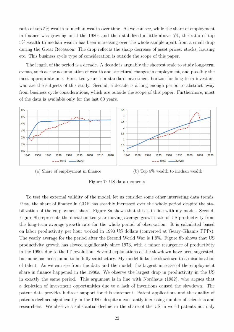
ratio of top 5% wealth to median wealth over time. As we can see, while the share of employmentin finance was growing until the 1980s and then stabilized a little above 5%, the ratio of top5% wealth to median wealth has been increasing over the whole sample apart from a small dropduring the Great Recession. The drop reflects the sharp decrease of asset prices: stocks, housingetc. This business cycle type of consideration is outside the scope of this paper.

The length of the period is a decade. A decade is arguably the shortest scale to study long-termevents, such as the accumulation of wealth and structural changes in employment, and possibly themost appropriate one. First, ten years is a standard investment horizon for long-term investors,who are the subjects of this study. Second, a decade is a long enough period to abstract awayfrom business cycle considerations, which are outside the scope of this paper. Furthermore, mostof the data is available only for the last 60 years.

(a) Share of employment in finance (b) Top 5% wealth to median wealth

Figure 7: US data moments

To test the external validity of the model, let us consider some other interesting data trends.First, the share of finance in GDP has steadily increased over the whole period despite the sta-bilization of the employment share. Figure 8a shows that this is in line with my model. Second,Figure 8b represents the deviation ten-year moving average growth rate of US productivity fromthe long-term average growth rate for the whole period of observation. It is calculated basedon labor productivity per hour worked in 1990 US dollars (converted at Geary–Khamis PPPs).The yearly average for the period after the Second World War is 1.9%. Figure 8b shows that USproductivity growth has slowed significantly since 1973, with a minor resurgence of productivityin the 1990s due to the IT revolution. Several explanations of the slowdown have been suggested,but none has been found to be fully satisfactory. My model links the slowdown to a misallocationof talent. As we can see from the data and the model, the biggest increase of the employmentshare in finance happened in the 1980s. We observe the largest drop in productivity in the USin exactly the same period. This argument is in line with Nordhaus (1982), who argues thata depletion of investment opportunities due to a lack of inventions caused the slowdown. Thepatent data provides indirect support for this statement. Patent applications and the quality ofpatents declined significantly in the 1980s despite a constantly increasing number of scientists andresearchers. We observe a substantial decline in the share of the US in world patents not only

22

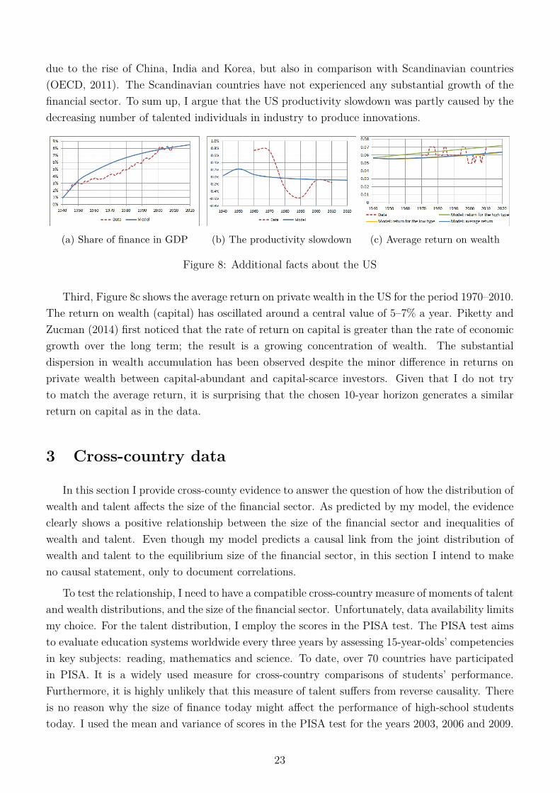
due to the rise of China, India and Korea, but also in comparison with Scandinavian countries(OECD, 2011). The Scandinavian countries have not experienced any substantial growth of thefinancial sector. To sum up, I argue that the US productivity slowdown was partly caused by thedecreasing number of talented individuals in industry to produce innovations.

(a) Share of finance in GDP (b) The productivity slowdown (c) Average return on wealth

Figure 8: Additional facts about the US

Third, Figure 8c shows the average return on private wealth in the US for the period 1970–2010.The return on wealth (capital) has oscillated around a central value of 5–7% a year. Piketty andZucman (2014) first noticed that the rate of return on capital is greater than the rate of economicgrowth over the long term; the result is a growing concentration of wealth. The substantialdispersion in wealth accumulation has been observed despite the minor difference in returns onprivate wealth between capital-abundant and capital-scarce investors. Given that I do not tryto match the average return, it is surprising that the chosen 10-year horizon generates a similarreturn on capital as in the data.

3 Cross-country data

In this section I provide cross-county evidence to answer the question of how the distribution ofwealth and talent affects the size of the financial sector. As predicted by my model, the evidenceclearly shows a positive relationship between the size of the financial sector and inequalities ofwealth and talent. Even though my model predicts a causal link from the joint distribution ofwealth and talent to the equilibrium size of the financial sector, in this section I intend to makeno causal statement, only to document correlations.

To test the relationship, I need to have a compatible cross-country measure of moments of talentand wealth distributions, and the size of the financial sector. Unfortunately, data availability limitsmy choice. For the talent distribution, I employ the scores in the PISA test. The PISA test aimsto evaluate education systems worldwide every three years by assessing 15-year-olds’ competenciesin key subjects: reading, mathematics and science. To date, over 70 countries have participatedin PISA. It is a widely used measure for cross-country comparisons of students’ performance.Furthermore, it is highly unlikely that this measure of talent suffers from reverse causality. Thereis no reason why the size of finance today might affect the performance of high-school studentstoday. I used the mean and variance of scores in the PISA test for the years 2003, 2006 and 2009.

23

I choose the mean and variance of 2009 science scores in the PISA test as a proxy for the momentsof talent distributions, because it includes the greatest number of countries. Moreover, this choicehardly affects the results, because PISA scores are highly correlated over time and disciplines: thecorrelation coefficients exceed 0.97.

To the best of my knowledge, there is no cross-country data on wealth inequality. Therefore,I have to use the income distribution as a proxy for the wealth distribution. Income inequalityis a fairly standard proxy for wealth inequality, but possibly underestimates wealth inequality.Income and wealth are not particularly well correlated either at the individual level for a givenpoint (Rodriguez et al. (2002) estimate the correlation between wealth and labor income to be0.27) or across countries (Fredriksen, 2012). However, if we measure the correlation over timebetween top income and wealth shares for a particular country, for example the US, we observethat the shares are highly correlated. The more concentrated are the shares, the higher are thecorrelations between them. In addition, the income shares are more volatile and tend to lead thewealth shares. We can see from Figure 9 that the dynamics of wealth shares closely track thedynamics of income shares for the US.

Figure 9: US top income and wealth sharesThe correlation for 10% (1%) is 0.52 (0.77)

To measure income inequality, I employ the Gini indexes from the Standardized World IncomeInequality Database (SWIID) and top income shares from the World Top Incomes Database. TheSWIID provides comparable Gini indexes of gross and net income inequality for 173 countries foras many years as possible from 1960. The World Top Incomes Database includes 45 countries forover a century for some countries.

The last issue is how to measure the size of finance. I construct the share of financial industryemployment in total employment using two datasets: the International Labour Organization (ILO)dataset, which contains employment by economic activity for 165 countries starting from 1968, and

24

the STAN Database for Structural Analysis, which contains industry-level data for employmentand output for 15 OECD countries from the 1970s up to the present.

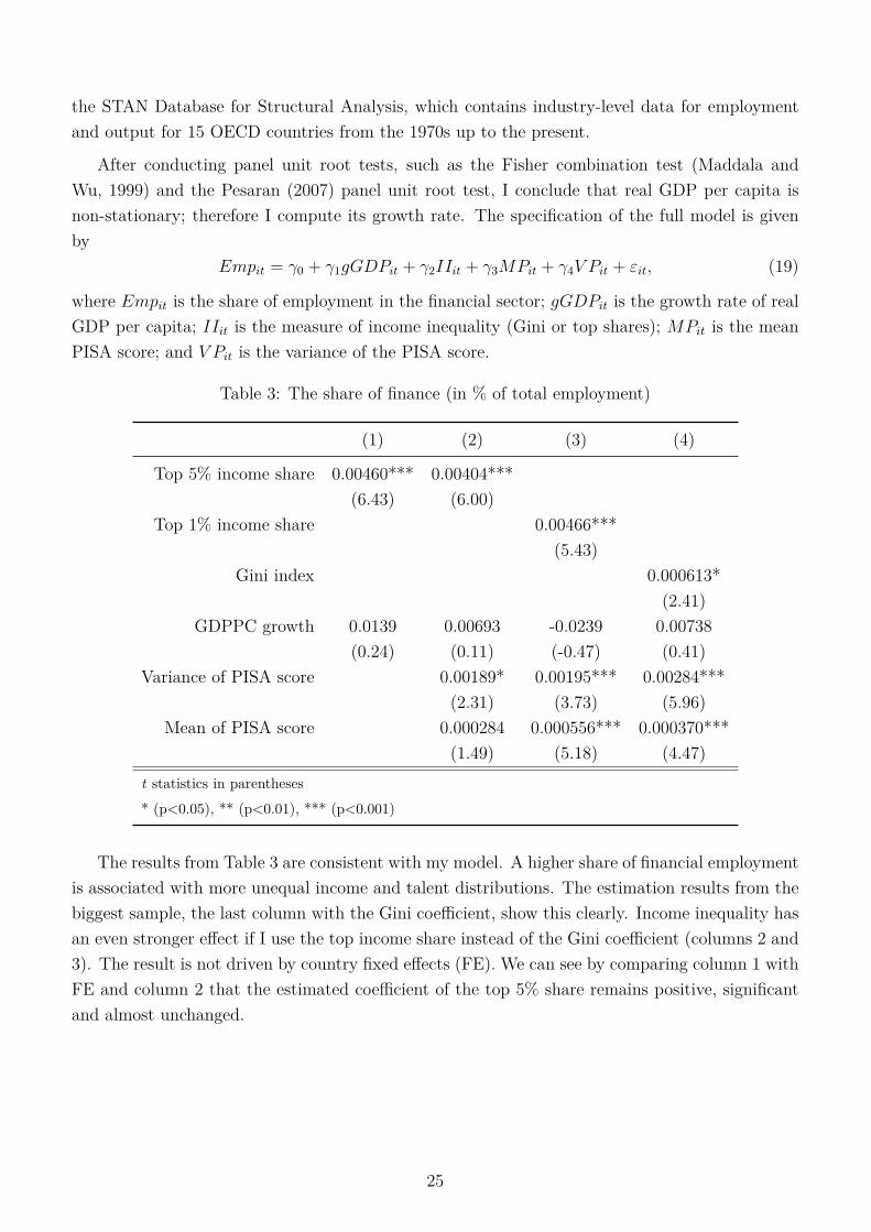
After conducting panel unit root tests, such as the Fisher combination test (Maddala andWu, 1999) and the Pesaran (2007) panel unit root test, I conclude that real GDP per capita isnon-stationary; therefore I compute its growth rate. The specification of the full model is givenby

Empit = γ0 + γ1gGDPit + γ2IIit + γ3MPit + γ4V Pit + εit, (19)

where Empit is the share of employment in the financial sector; gGDPit is the growth rate of realGDP per capita; IIit is the measure of income inequality (Gini or top shares); MPit is the meanPISA score; and V Pit is the variance of the PISA score.

Table 3: The share of finance (in % of total employment)

(1) (2) (3) (4)

Top 5% income share 0.00460*** 0.00404***(6.43) (6.00)

Top 1% income share 0.00466***(5.43)

Gini index 0.000613*(2.41)

GDPPC growth 0.0139 0.00693 -0.0239 0.00738(0.24) (0.11) (-0.47) (0.41)

Variance of PISA score 0.00189* 0.00195*** 0.00284***(2.31) (3.73) (5.96)

Mean of PISA score 0.000284 0.000556*** 0.000370***(1.49) (5.18) (4.47)

t statistics in parentheses

* (p<0.05), ** (p<0.01), *** (p<0.001)

The results from Table 3 are consistent with my model. A higher share of financial employmentis associated with more unequal income and talent distributions. The estimation results from thebiggest sample, the last column with the Gini coefficient, show this clearly. Income inequality hasan even stronger effect if I use the top income share instead of the Gini coefficient (columns 2 and3). The result is not driven by country fixed effects (FE). We can see by comparing column 1 withFE and column 2 that the estimated coefficient of the top 5% share remains positive, significantand almost unchanged.

25

4 Discussion and conclusion

In this section, I review the impact of the different assumptions on the outcome of the model:the inefficiency result and the inequality result. First, the inefficiency result states that thedecentralized equilibrium is generically inefficient. Second, the inequality result states that theendogenous growth of wealth inequality leads to the expansion of the financial sector.

Preferences and technology: First, for simplicity I assume the Cobb–Douglas productionfunction zαzkαk , which satisfies the supermodularity condition. However, the choice of a produc-tion function should not affect the results, because as long as z and k are not fully substitutable,the supermodularity condition holds. (See Topkis (1998) for a comprehensive mathematical treat-ment of supermodularity, and Milgrom and Roberts (1990) and Vives (2005) for applications ingame theory and economics.) According to the Becker–Brock theorem, the supermodularity con-dition implies that positive assortative matching is the first best allocation of my model. Hence,the results of the model remains unchanged as long as the production function is supermodular.Second, it should not be complicated to include labor as an additional input, but it would not addfurther insights on the questions addressed in this paper. It should not affect the choice of talentedagents, but it might have interesting implications for ordinary agents. Third, if we consider a riskaverse utility function instead of a risk neutral one, all agents would like to engage in risk sharing.If profit sharing and fund pooling are available options, the introduction of risk aversion does notchange anything, because expected and realized incomes are the same. If these options are notavailable, the impact of risk aversion is ambiguous. On the one hand, investors are willing to paya higher price for intermediated matching. The higher is the price, the higher is the income of abanker. On the other hand, due to higher uncertainty with respect to this income, risk aversionmakes a banking career a less attractive option.

Distribution of types: First, as long as within each period the wealth distribution is inde-pendent from the talent distribution, the investment decision is independent from the occupationalchoice. This makes the solution of the problem tractable. The consideration of the two-dimensionaljoint distribution of wealth and talent complicates the analysis enormously without much addi-tional insight for this particular question. Second, the fact that the constrained efficient allocationadmits only two values is an artifact of the discrete distribution of talent and the particular typeof information advantage for talented agents in finance: a banker with ability z can distinguishbetween ideas with productivity z and z′ < z. As long as both assumptions hold, the constrainedefficient allocation admits two values (zero and one-half) for each type of talent: the planner wouldfind it optimal either to keep the allocation under random matching or make it as close as possibleto the allocation under assortative matching by exhausting fully the opportunities for interme-diated matching. The allocation in the case of a continuous talent distribution would stronglydepend on the assumption made with respect to the impact of talent on agents’ productivity inthe two sectors. Third, I can provide intuition for the case of a continuous wealth distribution.The constrained efficient solution either have a positive share for all values of talent distribu-tion z or there exists a threshold in terms of ability z̄, that separates bankers and entrepreneurs.Calculating the decentralized equilibrium is a complicated numerical task.

26

Different types of frictions: First, this paper focuses on how the financial sector arises as aresult of one type of relevant friction, adverse selection. The financial sector clearly provides otheruseful functions to the economy: it allocates not only information, but also decision power and risk.On the theoretical side, the financial sector’s functions include: screening to mitigate the effectof adverse selection; monitoring to prevent the effects of moral hazard; auditing and punishmentto mitigate the effects of opportunistic behavior in the context of costly state verification. (SeeFreixas and Rochet (2008) for a precise survey of the theoretical literature.) Comparing my modelwith that of Bolton et al. (2011), who study moral hazard and the financial sector as a liquidityprovider, while I consider adverse selection and the financial sector as a classical intermediary, weboth obtain a similar result in terms of efficiency, but the mechanisms are substantially different.This suggests that the misallocation result might be a general feature of models with financialfrictions. Under the assumption that talent in finance affects the efficiency of monitoring, theinequality result is likely to survive as well. Second, The matching friction is clearly importantfor the inefficiency, because in the perfectly competitive market prices would take into accountthe negative externality, which arrised from the occupational choice. However, More a generalform of matching friction, many-to-one matching can be easily introduced into the environmentin at least two ways: through diminishing returns on capital and fixed costs of engaging withinvestors; or through making entrepreneurs’ bargaining power depend positively on the numberof investors in the market. Ceteris paribus, it is likely that many-to-one matching would lead tomore inefficiency in comparison to one-one matching. The more investors can be matched with oneentrepreneur, the fewer bankers are needed to restore efficiency. The income of a banker increaseswith the number investors matched with one entrepreneur. Hence, an even larger fraction oftalented agents is attracted to finance. The inefficiency should increase due to both a decline inthe constrained efficient fraction of talented agents in finance and a rise in the decentralized one.

Third, the issue of competition has been studied extensively. Monopoly is usually viewed as abad thing. However, in my framework one monopolistic firm in the financial sector might restoreefficiency, because it maximizes the total surplus by pushing all agents to their outside option. Themonopolist is always on the short side of the market. It would set the prices for its services to makeboth entrepreneurs and investors indifferent between paying for the services and being matched,and being randomly matched for free. On top of this, the monopolist can set wages for its workers(bankers) to make them indifferent between the two sectors. Hence, the monopolist could extractthe total surplus and would hire the efficient number of bankers. However, this possible advantageof a monopoly in the context of information provision does not overcome common disadvantagesof monopoly for a society.

4.1 Conclusion

This paper develops a new model of an economy with a financial sector and heterogeneousagents. The model sheds light on the role of the financial sector and its implication for the allo-cation of capital between entrepreneurs and the allocation of talent between finance and industry.Talent is important for both industry and the financial sector: more talent in industry means

27

more output is produced, while more talent in finance means capital is allocated more efficiently.The model establishes a link between the growth of the financial sector and the increase in wealthinequality. It shows that the market overproduces finance, but this inefficiency can be correctedby taxing bankers’ income. For the future, it would be interesting to quantitatively assess the sizeof this inefficiency and the importance of current wealth in limiting investment.

28

References

Bauer, C. and J. V. R. Mora (2014): “The Joint Determination of TFP and Financial SectorSize,” Working paper.

Becker, G. S. (1973): “A Theory of Marriage: Part I,” Journal of Political Economy, 81, 813–46.

Berkes, E., U. Panizza, and J.-L. Arcand (2012): “Too Much Finance?” IMF WorkingPapers 12/161, International Monetary Fund.

Bienz, C. and J. Hirsch (2011): “The Dynamics of Venture Capital Contracts,” Review ofFinance, 16, 157–195.

Bolton, P., T. Santos, and J. A. Scheinkman (2011): “Cream skimming in financialmarkets,” NBER Working Papers 16804, National Bureau of Economic Research, Inc.

Brunnermeier, M. K., T. M. Eisenbach, and Y. Sannikov (2012): “Macroeconomics withFinancial Frictions: A Survey,” NBER Working Papers 18102, National Bureau of EconomicResearch, Inc.

Buera, F. J. and Y. Shin (2013): “Financial Frictions and the Persistence of History: AQuantitative Exploration,” Journal of Political Economy, 121, 221 – 272.

Cahuc, P. and E. Challe (2012): “Produce Or Speculate? Asset Bubbles, OccupationalChoice, And Efficiency,” International Economic Review, 53, 1105–1131.

Chen, Q., I. Goldstein, and W. Jiang (2006): “Price Informativeness and Investment Sen-sitivity to Stock Price,” Review of Financial Studies, 20, 619–650.

Cooley, T. F., R. Marimon, and V. Quadrini (2013): “Risky Investments with LimitedCommitment,” NBER Working Papers 19594, National Bureau of Economic Research, Inc.

Durnev, A., R. Morck, and B. Yeung (2004): “Value-Enhancing Capital Budgeting andFirm-specific Stock Return Variation,” Journal of Finance, 59, 65–105.

Fredriksen, K. B. (2012): “Less Income Inequality and More Growth - Are they Compatible?Part 6. The Distribution of Wealth,” OECD Economics Department Working Papers No. 929,OECD.

Freixas, X. and J.-C. Rochet (2008): Microeconomics of Banking, 2nd Edition, MIT PressBooks, The MIT Press.

Gennaioli, N., A. Shleifer, and R. W. Vishny (2013): “Finance and the Preservation ofWealth,” NBER Working Papers 19117, National Bureau of Economic Research, Inc.

Gertler, M. and N. Kiyotaki (2010): “Financial Intermediation and Credit Policy in BusinessCycle Analysis,” in Handbook of Monetary Economics, ed. by B. M. Friedman and M. Woodford,Elsevier, vol. 3 of Handbook of Monetary Economics, chap. 11, 547–599.

29

Goldin, C. and L. F. Katz (2008): “Transitions: Career and Family Life Cycles of the Edu-cational Elite,” American Economic Review, 98, 363–69.

Goldsmith, R. (1995): Financial Structure and Development, vol. 1, Yale University Press.

Gordon, P. (2000): “The Americas,” Global Finance, 14.

Gourinchas, P.-O. and J. A. Parker (2002): “Consumption Over the Life Cycle,” Econo-metrica, 70, 47–89.

Greenspan, A. (2002): “World Finance and Risk Management,”http://www.federalreserve.gov/BoardDocs/Speeches/2002/200209253/default.htm.

Greenwood, R. and D. Scharfstein (2013): “The Growth of Finance,” Journal of EconomicPerspectives, 27, 3–28.

Hosios, A. J. (1990): “On the Efficiency of Matching and Related Models of Search and Unem-ployment,” Review of Economic Studies, 57, 279–98.

Hsieh, C.-T. and P. J. Klenow (2009): “Misallocation and Manufacturing TFP in China andIndia,” The Quarterly Journal of Economics, 124, 1403–1448.

Jovanovic, B. (2014): “Misallocation and Growth,” American Economic Review, 104, 1149–71.

Jovanovic, B. and B. Szentes (2013): “On the Market for Venture Capital,” Journal ofPolitical Economy, 121, 493 – 527.

Kaplan, S. N. and P. Stromberg (2003): “Financial Contracting Theory Meets the RealWorld: An Empirical Analysis of Venture Capital Contracts,” Review of Economic Studies, 70,281–315.

Kneer, C. (2012): “The Absorption of Talent into Finance: Evidence from U.S. Banking Dereg-ulation,” Job Market Paper of Tilburg University, 1–28.

Levine, R. (2005): “Finance and Growth: Theory and Evidence,” in Handbook of EconomicGrowth, ed. by P. Aghion and S. Durlauf, Elsevier, vol. 1 of Handbook of Economic Growth,chap. 12, 865–934.

Levinsohn, J. and A. Petrin (2003): “Estimating Production Functions Using Inputs toControl for Unobservables,” Review of Economic Studies, 70, 317–341.

Lucas, Robert E, J. and L. A. Rapping (1969): “Real Wages, Employment, and Inflation,”Journal of Political Economy, 77, 721–54.

Lucas, R. J. (1988): “On the mechanics of economic development,” Journal of Monetary Eco-nomics, 22, 3–42.

Luo, Y. (2005): “Do Insiders Learn from Outsiders? Evidence from Mergers and Acquisitions,”The Journal of Finance, 60, 1951–1982.

30

Maddala, G. S. and S. Wu (1999): “ A Comparative Study of Unit Root Tests with PanelData and a New Simple Test,” Oxford Bulletin of Economics and Statistics, 61, 631–52.

Mayer-Haug, K., S. Read, J. Brinckmann, N. Dew, and D. Grichnik (2013): “En-trepreneurial talent and venture performance: A meta-analytic investigation of SMEs,” ResearchPolicy, 1–23.

Merton, R. C. (1995): The Global Financial System: A Functioning Perspective, HarvardBusiness School Press.

MGI (2011): “Big data: The next frontier for innovation, competition, and productivity,” Themckinsey global institute report, The McKinsey Global Institute.

Michelacci, C. and J. Suarez (2004): “Business Creation and the Stock Market,” Review ofEconomic Studies, 71, 459–481.

Midrigan, V. and D. Y. Xu (2014): “Finance and Misallocation: Evidence from Plant-LevelData,” American Economic Review, 104, 422–58.

Milgrom, P. and J. Roberts (1990): “Rationalizability, Learning, and Equilibrium in Gameswith Strategic Complementarities,” Econometrica, 58, 1255–77.

Murphy, K. M., A. Shleifer, and R. W. Vishny (1991): “The Allocation of Talent :Implications for Growth,” The Quarterly Journal of Economics, 106, 503–530.

Nash, J. (1950): “The Bargaining Problem,” Econometrica, 18, 155–162.

——— (1953): “Two-Person Cooperative Games,” Econometrica, 21, 128–140.

Nordhaus, W. D. (1982): “Economic policy in the face of declining productivity growth,”European Economic Review, 18, 131–157.

Obama, B. (2009): “The President Explains His Larger Vision on the Economy,”http://www.whitehouse.gov/video/The-President-Explains-His-Larger-Vision-on-the-Economy.

OECD (2011): “OECD Science, Technology and Industry Scoreboard,” Oecd report, OECD.

Pesaran, M. H. (2007): “A simple panel unit root test in the presence of cross-section depen-dence,” Journal of Applied Econometrics, 22, 265–312.

Philippon, T. (2010): “Financiers versus Engineers: Should the Financial Sector be Taxed orSubsidized?” American Economic Journal: Macroeconomics, 2, 158–182.

Philippon, T. and A. Reshef (2012): “Wages and Human Capital in the U.S. Finance Industry:1909–2006,” The Quarterly Journal of Economics, 127, 1551–1609.

Piketty, T. and G. Zucman (2014): “Capital is Back: Wealth-Income Ratios in Rich Coun-tries, 1700-2010,” The Quarterly Journal of Economics.

31

Restuccia, D. and R. Rogerson (2008): “Policy Distortions and Aggregate Productivitywith Heterogeneous Plants,” Review of Economic Dynamics, 11, 707–720.

Rodriguez, S. B., J. Diaz-Gimenez, V. Quadrini, and J.-V. Rios-Rull (2002): “Updatedfacts on the U.S. distributions of earnings, income, and wealth,” Quarterly Review, 2–35.

Rogerson, R. (2008): “Structural Transformation and the Deterioration of European LaborMarket Outcomes,” Journal of Political Economy, 116, 235–259.

Romer, P. M. (1986): “Increasing Returns and Long-Run Growth,” The Journal of Politicaleconomy, 94, 1002–1037.

Sahlman, W. A. (1990): “The structure and governance of venture-capital organizations,” Jour-nal of Financial Economics, 27, 473–521.

Santarelli, E., L. Klomp, and A. Thurik (2006): “Gibrat’s Law: An Overview of the Em-pirical Literature,” in Entrepreneurship, Growth, and Innovation, ed. by E. Santarelli, SpringerUS, vol. 12 of International Studies in Entrepreneurship, 41–73.

Schumpeter, J. A. (1934): The Theory of Economic Development: An Inquiry into Profits,Capital, Credit, Interestand the Business Cycle, Transaction Publishers.

Shu, P. (2012): “Essays on Innovation, Productivity, and Talent Allocation,” MIT Job MarketPaper.

Tobin, J. (1984): “On the efficiency of the financial system,” Lloyds Bank Review, 153, 1âĂŞ15.

Topkis, D. M. (1998): Supermodularity and Complementarity, Princeton University Press, firstedition ed.

Vives, X. (2005): “Complementarities and Games: New Developments,” Journal of EconomicLiterature, 43, 437–479.

Volcker, P. (2009): “Paul Volcker: Think More Boldly,”http://online.wsj.com/articles/SB10001424052748704825504574586330960597134.

Wadhwa, V., B. A. Rissing, and G. Gereffi (2006): “Industry Trends in EngineeringOffshoring,” report, Duke University.

Yang, F. (2009): “Consumption over the Life Cycle: How Different is Housing?” Review ofEconomic Dynamics, 12, 423–443.

32

List of Figures

1 The growth of the financial sector in the US . . . . . . . . . . . . . . . . . . . . . 2

2 Model without bankers . . . . . . . . . . . . . . . . . . . . . . . . . . . . . . . . . 8

3 Model with bankers . . . . . . . . . . . . . . . . . . . . . . . . . . . . . . . . . . . 10

4 Tax on financial income vs. inefficiency . . . . . . . . . . . . . . . . . . . . . . . . 17

5 Fraction of bankers vs. bargaining power of entrepreneur . . . . . . . . . . . . . . 18

6 Fraction of bankers vs. bargaining power of entrepreneur . . . . . . . . . . . . . . 18

7 US data moments . . . . . . . . . . . . . . . . . . . . . . . . . . . . . . . . . . . . 22

8 Additional facts about the US . . . . . . . . . . . . . . . . . . . . . . . . . . . . . 23

9 Top income and wealth shares . . . . . . . . . . . . . . . . . . . . . . . . . . . . . 24

List of Tables

1 The simple example . . . . . . . . . . . . . . . . . . . . . . . . . . . . . . . . . . . 9

2 Parameter values . . . . . . . . . . . . . . . . . . . . . . . . . . . . . . . . . . . . 21

3 The share of finance (in % of total employment) . . . . . . . . . . . . . . . . . . 25

4 The size of private equity . . . . . . . . . . . . . . . . . . . . . . . . . . . . . . . . 39

5 Private equity funds . . . . . . . . . . . . . . . . . . . . . . . . . . . . . . . . . . 40

6 US real asset returns . . . . . . . . . . . . . . . . . . . . . . . . . . . . . . . . . . 40

7 Wealth distribution in the US . . . . . . . . . . . . . . . . . . . . . . . . . . . . . 40

33

A Appendix

A.1 Proof of Proposition 1

The proof is organized in the following way. First, I show that as long as γ is greater than 1/2,aggregate output Y (γ) decreases with γ. Second, depending on other parameters, Y (γ) is either astrictly increasing, or strictly decreasing, or a non-monotonic function of γ for the whole intervalγ ∈ [0, 1/2]. In the latter case, I prove that the function is a convex function for γ ∈ [0, 1/2].

For γ > 1/2, aggregate output Y (γ) is given by

Y (γ) = (βi−(1−γ)βe)(1−(1−γ)βe) (1− βe)FLH + (1−βi)

1−(1−γ)βe (1− βe)FLL + (1− γ)βeFHH . (20)

To show whether it is increasing or decreasing, we take the derivative of (20) with respect to γ:

∂Y∂γ|γ>1/2 = βe(1−βi)(1−βe)

(1−(1−γ)βe)2 FLH − βeFHH − βe(1−βi)(1−(1−γ)βe)2FLL. (21)

We need to estimate the sign of expression (21). Since F is a supermodular function, FLL ≥ 0and FHH ≥ FLH . Hence

∂Y∂γ|γ>1/2 ≤ βe(1−βi)(1−βe)

(1−(1−γ)βe)2 − βe. (22)

Expressing the two terms on the right-hand side of condition (22) using a common denominator,then replacing γ in the numerator by 1/2 (this value makes the numerator as small as possible),and finally expanding, we obtain:

∂Y∂γ|γ>1/2 ≤ βe (1−βe)(1−βi)−(1−βe+γβe)2

(1−(1−γ)βe)2 ≤ βe (1−βe)(1−βi)−(1−βe+0.25(βe)2)(1−(1−γ)βe)2 ≤ 0. (23)

Here is the end of the proof of the first part. To prove the second part, I follow a similar procedure.I calculate the first derivative and restrict my attention to the case in which the first derivative isneither positive or negative for the whole interval γ ∈ [0, 1/2]. Then, I show that in this case thesecond derivative is positive, i.e. the function is convex.

For γ ∈ [0,1/2], the aggregate output Y (γ) is given by

Y (γ) = (βi−γβe)(1−γβe) [(1− 2γ)βeFHH + (1− βe)FLH ] +

(1−βi)(1−γβe) [(1− 2γ)βeFHL + (1− βe)FLL] + γβeFHH .

(24)

Calculating the first derivative from (24), we obtain

∂Y∂γ|γ∈[0,1/2] = 1

(1−γβe)2 [βeFHH (1 + 2γβe − (γβe)2 + βiβe − βe + 2βi)−(1− βe)βe(1− βi)(FLH − FLL)− (2− βe)βe(1− βi)FHL] .

(25)

The first derivative is negative for the whole interval γ ∈ [0, 1/2] if

βeFHH (1 + 2γβe − (γβe)2 + βiβe − βe + 2βi)− (2− βe)βe(1− βi)FHL <(1− βe)βe(1− βi)(FLH − FLL).

(26)

34

The left-hand side of inequality (26) increases with γ, while the right-hand side of inequality (26)is independent of γ. Hence if inequality (26) holds for γ = 1/2, it holds for any γ ∈ [0, 1/2].

[βeFHH (1− 0.25(βe)2 + βiβe + 2βi)−(1− βe)βe(1− βi)(FLH − FLL)− (2− βe)βe(1− βi)FHL] < 0

(27)

If inequality (27) holds, the first derivative is negative. In the opposite case, the sign of thederivative is unknown. Inequality (27) imposes the restriction on the set of exogenous parameters.

We now calculate the second derivative and check its sign:

∂2Y∂γ2 |γ∈[0,1/2] = 2βe

(1−γβe)3 [βeFHH (1 + βiβe + 2βi)−(1− βe)βe(1− βi)(FLH − FLL)− (2− βe)βe(1− βi)FHL] .

(28)

If the second derivative is positive, the function is convex. I need to show that the right-handside of (28) is positive. As we have seen, when inequality (27) does not hold, the sign of the firstderivative is unknown, but it imposes the restriction on the set of exogenous parameters. Thisis the case in which we need to know the sign of the second derivative. We can estimate theright-hand side using the complementary inequality to condition (27):

βeFHH (1 + βiβe + 2βi)− (2− βe)βe(1− βi)FHL − (1− βe)βe(1− βi)(FLH − FLL) ≥βeFHH0.25(βe)2 > 0.

(29)

This completes the proof of the first part. We show that the sign of the first derivative is eithernegative or unknown. In the case in which it is unknown, we prove that the second derivative isstrictly positive. Hence, the solution of the planner’s problem can be either 0 or 1/2.

A.2 Proof of Proposition 2

The characterization of a decentralized equilibrium is the following triplet: two prices and theshare of talented agents in finance (pi, pe, γ). We have:

pi ≤ (1− δ)(FHH − di(γ)− de(γ)),pe ≤ δ(FHH − di(γ)− de(γ)),

min{γ,1−γ}γ

(pi + pe) = δ (FHH − di(γ)) + (1− δ)de(γ)− pe.(30)

As a reminder, there are three types of agents who affect the solution of intermediated match-ing: capital-abundant investors, talented entrepreneurs and bankers. The number of investors isβi, the equilibrium number of bankers is γβe, and the equilibrium number of entrepreneurs is(1 − γ)βe. There are two markets and consequently two prices that clear them: entrepreneur–banker and investor–banker. System (30) should be solved differently depending on who is on theshort side of both markets: capital-abundant investors, talented entrepreneurs or bankers. I showthat a solution exists only if capital-abundant investors are on the long side of the investor–bankermarket. Furthermore, the condition γ∗ = 1/2 imposes an additional restriction on the set of ex-ogenous parameters, and eliminates a possible solution with bankers being on the short side with

35

respect to talented entrepreneurs on the entrepreneur–banker market. However, the solution doesnot always exist. I state the existence condition as well.

The system can be solved backwards. First, we need to define who is on the short side of themarket: capital-abundant investors, talented entrepreneurs or bankers. Second, I solve the randommatching problem for a given size of the financial sector γβe to determine the outside options ofcapital-abundant investors di(γ) and talented entrepreneurs de(γ) in the case in which they decidenot to be matched with a high-type counterpart with certainty through a banker. Third, usingthe solution of random matching as outside options, I solve the intermediated matching problemfor capital-abundant investors and talented entrepreneurs.

Capital-abundant investors are on the short side: The number of capital-abundantinvestors is lower than the number of bankers who provide services for investors βi < γβe. Hence,competition among bankers drives the price pi down to zero. If the number of bankers is greaterthan the number of talented entrepreneurs, the bankers’ income is zero, because prices for theirservice are zero.

Furthermore, the number of bankers cannot be greater than the number of talented en-trepreneurs. Otherwise, bankers’ income is zero, and any talented agent strictly prefers to bean entrepreneur. Thus, if capital-abundant investors are on the short side of the investor–bankermarket, the share of talented agents in finance must be γ ≤ 1/2.

If γ ≤ 1/2 and pi = 0, the system (30) take the following form:

pe = δ(FHH − di(γ)− de(γ)),2pe = δ (FHH − di(γ)) + (1− δ)de(γ).

(31)

Substituting prices, system (31) collapses to one condition (32)

δFHH = δdi(γ) + (1 + δ)de(γ). (32)

Condition (32) does not hold unless δ = 0. Hence, capital-abundant investors cannot be on theshort side in equilibrium.

Capital-abundant investors are on the long side: The number of capital-abundantinvestors is higher than the number of bankers who provide services for investors βi ≥ γβe.Hence, bankers push capital-abundant investors to their outside options. The first equation ofsystem (30) becomes an equality. Two cases are possible.

First, if the number of bankers is lower than the number the talented entrepreneurs γ ≤ 1/2,1− 2γβe talented entrepreneurs are left for random matching. We assume that investors have noaccess to a storage technology, while entrepreneurs have no opportunity for outside borrowing.Thus, the outside options for a random match—the set D in (5)—are (0, 0). The solution ofthe Nash bargaining problem gives the value of random matching for capital-abundant investors,which is equal to the probability of matching with somebody 1−2γβe

1−γβe multiplied by the sum of twoterms: the probability of matching with a talented entrepreneur (1−2γ)βe

1−2γβe multiplied by the fractionof the project’s output received by the investor (1− δ)FHH ; and the probability of matching with

36

an ordinary entrepreneur 1−βe

1−2γβe multiplied by the fraction of the project’s output received by theinvestor (1− δ)FLH :

di = 1− 2γβe1− γβe

1− δ1− 2γβe [(1− 2γ)βeFHH + (1− βe)FLH ] . (33)

A similar expression can be obtained for the talented entrepreneur. The probability of matchingwith somebody for a talented entrepreneur is equal to 1, so

de = δ

1− γβe[(βi − γβe)FHH + (1− βi)FHL

].

Due to the supermodularity of the output function, sorting is possible. There exists a separatingequilibrium such that the incentive compatibility constraint for the capital-scarce investor holds(the low type has no incentive to mimic the high type). The capital-abundant investor is indifferentbetween being randomly matched and being matched by a banker, while the capital-scarce investoris strictly better off under random matching. In this case, the system (30) takes the form below:

pi = (1− δ)(FHH − di(γ)− de(γ)),pe = δ(FHH − di(γ)− de(γ)),

(pi + pe) = δ (FHH − di(γ)) + (1− δ)de(γ).(34)

Surprisingly, as long as γ ≤ 1/2, the income of a banker is an increasing function of the number ofbankers, while the income of an entrepreneur is a decreasing function of the number of bankers. Therise of bargaining power δ has no effect on the banker’s income and a positive one on entrepreneurialincome. The solution of the system (34) is linear in δ:

γ̃ = δ

[1βe

+ 1− βeβe

FHH − FLHFHH

− 2(1− βi)βe

FHH − FHLFHH

]− 1− βe

βeFHH − FLH

FHH. (35)

There exist two thresholds δ̄ > 0, such that γ̃ = 0, and δ̃ > 0, such that γ̃ = 1/2:

δ̄ = (1− βe)(FHH − FLH)(1− βe)(FHH − FLH) + (2βi − 1)(FHH − FHL) + FHL

, (36)

δ̃ = (1− βe/2)FHH − (1− βe)FLH(1− βe)(FHH − FLH) + (2βi − 1)(FHH − FHL) + FHL

. (37)

Depending on parameter values, both δ̄ and δ̃ can potentially be greater than 1. The solution γ̃exists only for δ ∈ [min{δ̄, 1},min{δ̃, 1}]. The solution γ̃ exists as long as δ̄ ≤ 1. Using expression(36), the latter can be rewritten as follows:

(2βi − 1)(FHH − FHL) + FHL ≥ 0. (38)

Second, the number of bankers is greater than or equal to the number of talented entrepreneursγ ≥ 1/2. Thus, all talented entrepreneurs are matched by bankers. The number of capital-abundant investors βe(1 − γ) are matched by bankers. In this case, the solution of the Nashbargaining problem for random matching is given by

di = (1− βe)1− βe(1− γ)(1− δ)FLH , (39)

de = δ

1− βe + γβe

[(βi − βe + γβe)FHH + (1− βi)FHL

]. (40)

37

If the number of bankers is greater than the number of talented entrepreneurs, competition amongbankers drives the price pi down to zero. In this case, system (30) takes the form below:

pi = (1− δ)(FHH − di(γ)− de(γ)),pe = 0,

1−γγpi = δ (FHH − di(γ)) + (1− δ)de(γ).

(41)

As we can see, the banker’s income is a decreasing function of the bargaining power δ, whileentrepreneurial income is an increasing function of δ. Furthermore, the expected income of abanker grows with γ. System (41) can be expressed in the form of a quadratic equation in γ:

γ2 +[(1− δ) (1−βe)

βeFHH−FLH

FHH+ δ−βe

βe + δ(1− δ)]γ−

−(1− δ)2 (1−βe)βe

FHH−FLH

FHH− (1− βi)(1− δ) δ

βeFHH−FHL

FHH= 0.

(42)

The solution of quadratic equation (42) contains two roots, but one root is always negative. Forthe solution to exist, the second root has to be greater than 1/2. Let γ̂ be the positive solution of(42). This solution exists as long as

δ(1 + βe(1− δ))4(1− δ) ≤ (1− βi)δFHH − FHL

FHH+ (1− βe)FHH − FLH

FHH(1/2− δ). (43)

Analyzing condition (43), we can conclude that the condition is likely to be satisfied when: thedispersion of wealth kH/kL is high; the share of capital-abundant investors βi is low; and thebargaining power of entrepreneurs δ is relatively low. Furthermore, if δ ≤ 1/2, condition (43)is likely to be satisfied when the dispersion of talent is high and the share of talented agents βe

is low. When condition (43) is satisfied with equality, it can be rewritten as the definition of δ̂defined in Proposition 2.

The constrained efficient allocation is γ∗ = 1/2: This implies that ∆Y given by expres-sion (3) is positive and can be rewritten in the following form:

(2βi − 1)(FHH − FHL) + FHL < −2(1− βi)(1− βe)

2− βe (FLH − FLL). (44)

The right-hand side of inequality (44) is negative, therefore its left-hand side is negative as well.If we compare the left-hand side of (44) with the left-hand side side of expression (38), they areexactly the same. Hence, if γ∗ = 1/2, the solution γ̃ does not exist.

A.3 The solution of the decentralized equilibrium if γ∗ = 0

In this section, I show the solution of the decentralized equilibrium in the case in which theconstrained efficient allocation is 0. The proposition below summarizes the case:

Proposition 3. If the constrained efficient allocation is γ∗ = 0, then both equilibria with few γ̃ andmany γ̂ bankers are possible. In this case, there is a range of δ ∈ [δ̃, 1], such that the decentralizedequilibrium is constrained efficient.

38

Proof : As shown in appendix A.2, the solution γ̂ exists as long as condition (43) holds, andit does not depend on whether the constrained efficient allocation is 0 or 1/2; the solution γ̃ doesnot exist if γ∗ = 1/2. The solution γ̃ exists as long as δ̄ < 1, defined by expression (36). Thelatter is likely to be satisfied if γ∗ = 0.

B Appendix

B.1 Private banking and private equity finance

This subsection introduces an alternative way of calibrating the model. Most global banks,such as Credit Suisse, Barclays, BNP Paribas, Citibank, Deutsche Bank, HSBC, JPMorgan Chaseand UBS, have a separate business unit with dedicated teams of client advisors and productspecialists exclusively for high-net-worth individuals. They provide a wide range of investmentopportunities, including bonds, stocks and more importantly private equity finance.

Private equity is an important channel through which long-term investments are made. It hasgrown steadily over the past three decades, and today private equity funds worldwide manageover $1 trillion. For some countries, such as Israel, the US and the UK, private equity accountsfor more than 5% of total investment (see Table 4 for details).

Table 4: The size of private equity

% GDP % Investment2010 2011 2010 2011

Israel 0.63 2.09 3.50 10.45UK 1.13 0.75 7.53 5.00US 0.9 0.98 5.00 5.44

China 0.16 0.33World 0.30 1.58

I would like to convince the reader that the matching assumption holds for private equity. Asmall private equity fund provides an opportunity to invest in a few companies over a long-termhorizon for a small number of wealthy investors. As we can see from Table 5, private equity fundstypically employ 12 professionals. These professionals select one or two companies each for the fundto invest in. Investments are large (over $50 million). Investors are wealthy and expected to investover a long-term horizon. The minimum required commitment rises from a median of $1 million forfunds of $100 million or less, up to a median of $10 million for funds of $1 billion or more. Thereis no active market for private equity positions, making these investments illiquid and difficultto value. Private equity funds typically have horizons of 10–13 years, during which the investedcapital cannot be redeemed. Furthermore, based on the sample of firms from the PricewaterhouseNational Venture Capital Survey, Gordon (2000) shows that 71.32% of firms reported they had

39

received more than one offer to invest from venture capitalists. The mean number of offers was3.18. This means entrepreneurs have a choice about which venture capitalists invest in theircompanies, but this choice is rather limited and matching plays an important role.

Table 5: Private equity funds

Number of Size ($ mn)N professionals investments I/P Fund Investment

VC 94 9 20 2 225 11.25Buyout 144 13 12 1 600 50

Given the long-term horizon and the high entry costs, the question is why investors are willingto engage in these investments. Investors are compensated well by substantially higher returns.Table 6 shows that the return from an investment in private equity funds is three times higherthan in stocks. We can see the comparison with inflation and the returns on other assets: stocks,gold, T-bills etc.

Table 6: US real asset returns

Period PEF S&P TBond Gold Inflation

1997-2011 9.2% 3.2% 0.4% 7.0% 2.4%1975-2011 7.5% 1.3% 4.0% 4.2%

The first important ingredient of the model is the wealth distribution. If we look at Table 7,we can conclude that at most 5% of households in the US can afford to invest at least $1 millionfor the horizon of ten years. I target 5% as the share of capital-abundant investors.

Table 7: Wealth distribution in the US

1962 1983 1989 1998 2001 2007 2010

Average 194 284 326 362 468 564 464Median 52 73 78 81 91 108 57Top 20% 786 1157 1361 1507 1976 2397 2062Top 5% 2120 3190 3841 4273 5542 6973 5842Top 1% 6491 9599 12176 13650 15627 19486 164391% to median 125 131 156 168 173 181 288

The second important ingredient of the model is the distribution of talent. The most chal-lenging exercise is to calibrate it. I use three different proxies. First, based on US firm-level dataI estimate the moments of the productivity distribution in the US. Second, based on data ondifferent test scores from the National Longitudinal Survey of Youth 1997 (NLSY97), I estimatesthe moments of the IQ distribution in the US. Finally, since my model contains only two levels of

40

talent, we might think of these as being college graduates and high-school graduates. Therefore,I use data on the share of college graduates over time as a proxy for the increase in the supply oftalent (skills).

41