Trade and the Allocation of Talent with Capital MarketImperfections.

Roberto Bonfatti, Oxford UniversityMaitreesh Ghatak, LSE∗

July 2012

Abstract

Trade liberalization in the 1980s and 1990s has been associated with a sharp increase inthe skill premium in both developed and developing countries. This is in apparent conflictwith neoclassical theory, according to which trade should decrease the relative return onthe relatively scarce factor, and thus decrease the skill premium in skill-scarce developingcountries. We develop a simple model of trade with talent heterogeneity and capital marketimperfections, and show that trade can increase the skill premium in a skill-scarce Souththat opens up to a skill-abundant North, both in the short run as well as in the long run.We show that trade has two effects: it reduces the skilled wage, and therefore drives nontalented agents out of the skilled labor force. It also reduces the cost of subsistence, therebyallowing the talented offspring of unskilled workers to go to school. This compositional effecthas a positive effect on the observed skill premium, potentially strong enough to outweighthe decrease in the skilled wage. In our framework, trade liberalization may trigger anincrease in the skill-premium in both the North and the South.

JEL Codes: F16, O15, O16Keywords: Trade Liberalization, Talent Heterogeneity, Skill Premium, Credit Market

Frictions.

∗We thank two anonymous referees, and the Co-Editor, Kala Krishna, for very helpful comments. We alsothank Chiara Binelli, Paul Beaudry, Nina Pavcnik, Priya Ranjan, Steve Redding, Eric Verhoogen for helpfulfeedback, and Sutanuka Roy for excellent research assistance. The second author would like to thank STICERDfor financial support.

1

1 Introduction

One of the most important results in Heckscher-Ohlin models of international trade, the Stolper-

Samuelson theorem, predicts that when a country opens up to international trade - and thus, its

relative price of skill-intensive goods decreases - the return of unskilled workers should increase,

relative to the return of skilled workers.1 This prediction has been confirmed in a number of

unskilled labor-abundant “early globalizers” (such as Italy, Singapore, South Korea and Taiwan)

where trade has increased the unskilled wage relative to the skilled wage (thus decreasing the

skill premium). However in the case of unskilled labor-abundant countries that have globalized

in the 1980s and 1990s (such as most of Latin America, India and Hong Kong), trade seems to

have increased the skill premium, rather than reducing it.2

This fact, sometimes called the “skill premium puzzle”, has attracted a fair bit of attention.

On the one hand, the trade literature has sought to reconcile the Latin American experience with

Heckscher-Ohlin theory (HO from now on) by arguing that trade liberalization disproportionately

affected unskilled labor-intensive industries (Revenga, 1997), or that countries such as China,

Indonesia and Pakistan made the world outside Latin America actually unskilled labor-abundant

(Davis, 1996; Wood, 1999). In these contexts, HO theory would correctly predict an increase in

the skill premium in Latin America. One problem with these interpretations is that they predict

that skill intensity should have decreased across sectors in Latin America, a prediction that has

not been confirmed in the data.3 In response to these shortcomings, the literature has turned to

alternative trade models to explain the generalized increase in wage inequality,4 or to non-trade

1More precisely, the Stolper-Samuelson theorem predicts that the real return of unskilled workers shouldincrease, whereas the real return of skilled workers should decrease.

2This has been documented by micro-studies of at least 7 countries: Chile, Mexico, Colombia, Argentina,Brazil, India and Hong Kong. See the survey by Goldberg and Pavcnik (2007) for more details.

3See Goldberg and Pavcnik (2007, p. 59) for a list of empirical papers finding that skill intensity has increasedacross most industries in Latin America.

4For example, Feenstra and Hanson (1996) study the impact of trade liberalization when this is associated withsignificant outsourcing flows from North to South. They find that this specific type of liberalization may increasethe skill premium in both countries. Verhoogen (2008) builds a heterogeneous firm trade model where firms differin productivity and quality of production, and shows that quality upgrading following trade liberalization mayresult in a higher relative white-collar wage and higher sectoral wage inequality. Helpman et al (2010) also workwith a heterogenous firm model, but emphasize labor market frictions and differences in workforce compositionacross firms. They show that trade increases the dispersion of wages paid by firms, at least in the short run. Foran excellent review of these and other recent theoretical developments, see Harrison et al (2011).

2

explanations, such as, skill biased technical change.

In this paper, we propose a way to reconcile a traditional HO model of trade liberalization

between an unskilled labor-abundant South and a skill labor-abundant North with an increase of

the skill premium in the South as well as in the North. We do so by enriching the baseline model

with talent heterogeneity, human capital accumulation, and credit constraints. The literature on

trade liberalization in the presence of credit constraints (discussed below in detail) has shown

that trade may increase human capital accumulation by relaxing the credit constraints faced by

the poor, thereby improving their access to the education system. We show that when this is

the case, trade may improve the allocation of talent to the skilled labor force, both in the short

and in the long run. This compositional effect generates an upward pressure on the observed

skilled wage, which can be strong enough to overturn the Stolper-Samuelson prediction of a

lower skill premium in the South following trade liberalization. While reconciling the Stolper-

Samuelson theorem with the Latin American experience, our model preserves the other main

features of standard HO theory, including the fact that all industries in the South become more

skill-intensive after trade liberalization.5

Our mechanism works as follows. Because of capital market imperfections, young agents

cannot borrow to pay for their subsistence while attending school. Thus, only those whose

parents have a high wage can possibly go to school. In an economy with little human capital,

unskilled wages are low, and the cost of subsistence is high relative to the income of unskilled

workers. This creates one equilibrium in which there are few skilled workers, the skilled wage is

high, and all and only the offspring of skilled workers go to school. With heterogeneous talent,

this equilibrium is “bad” in efficiency terms, in that many talented offspring of unskilled workers

are prevented from going to school while many offspring of skilled workers go to school despite

being non-talented. This is in contrast to a “good” equilibrium in which there are many skilled

workers, the skilled wage is low, and all and only the talented workers go to school independently

5Another HO feature that is preserved in our model is the fact that labor reallocates towards labor-intensiveindustries in the South. While Verhoogen (2008) finds evidence of such reallocation for Mexico, Wacziarg andWallack (2004) find little evidence of labor re-allocation across sectors following trade liberalization in a sampleof 20 countries. Importantly, we argue that our mechanism would survive if we allowed for labor market frictions(such as a high cost of firing) to slow down the inter-sectoral reallocation of labor. Rigid labor market havebeen indicated as one of the main reasons why labor reallocation to industries where a country has comparativeadvantage has been very slow in many countries (see, for example, Kambourov, 2009).

3

of the economic status of their families.

We consider an economy that is skill-scarce because it is stuck at the bad equilibrium, and

study its reaction to the liberalization of trade with a skill-abundant world. By putting a

downward pressure on the skilled wage, trade may induce many non-talented skilled workers

to drop out of the skilled labor force. At the same time, it reduces the cost of subsistence for

unskilled workers, thus making it easier for their offspring to go to school. Because many of these

previously-excluded agents are highly talented, they may still find it optimal to join the skilled

labor force despite the trade-induced drop in the skilled wage. These two effects may move the

economy from its initial equilibrium to the good equilibrium, thus increasing the average quality

of the skilled labor force. This creates an upward force on the average observed skill premium,

that can more than compensate the negative effect of trade on the skilled wage. Thus, the skill

premium may increase in the skill-scarce country, both in the short run and in the long run.6

Our results suggest that the Stolper-Samuelson theorem needs to be modified in the context of

talent heterogeneity and imperfect credit markets, to account for the possibility of compositional

changes in the skilled labor force.

The literature on trade with capital market imperfections is now quite large. An important

part of it has focused on how comparative advantage and the pattern of trade are determined

by cross country heterogeneity in the efficiency of capital markets (see for example Kletzer and

Bardhan, 1987; Wynne, 2005; and Manova, 2008). Although our result is compatible with the

idea that comparative advantage in the export of skill-intensive products may be driven by dif-

ferences in capital market development, the focus of our paper is different. More connected to

our paper is the literature on trade liberalization and skill acquisition in the presence of credit

market frictions. This literature has studied several ways in which trade liberalization may af-

fect domestic credit constraints and, through this channel, skill acquisition. In an important

contribution Cartiglia (1997) shows that trade liberalization reduces the cost of schooling in a

skill-scarce South by reducing the relative wage of skilled workers a la Stolper-Samuelson, thus

making it easier for poor, credit constrained households to send their children to school. This

6A similar result applies in the two-country version of the model (see the working paper version of the paper:Bonfatti and Ghatak, 2011). There, we show that trade may increase the skill premium in the skill-scarce country,while it always increases it in the skill-abundant country.

4

effect may be large enough to offset the standard result that trade discourages the accumulation

of the scarce factor (via the Stolper-Samuelson decrease in its relative return; see Findlay and

Kierzkowski, 1983, and Grossman and Helpman,1991), thus creating a positive association be-

tween trade liberalization and skill accumulation in South. Ranjan (2001a, 2003) enriches the

setting in Cartiglia (1997) by studying how trade may affect credit constraints also through the

distribution of income and wealth. The main intuition here is that trade increases (decreases) the

wage income and long-run wealth of unskilled workers in South (North). Assuming that credit

constraints affect mainly the children of unskilled workers, trade results in a lessening of credit

constraints in South, and a strengthening of credit constraints in North (unless credit constraints

are institutionally less present in North).7 Building on this latter result, Chesnokova and Krishna

(2009) show that the supply of skill-intensive goods in North may actually decrease following

trade liberalization, due to a strengthening of credit constraints. This carries the intriguing

implication that trade may decrease welfare in such a country.8

We borrow from this literature the basic insight that, in the presence of credit constraints,

trade may increase the supply of skilled labor in South. In particular, our result that trade may

shift South from a low-skill equilibrium to a high-skill equilibrium in the long run has much

in common with the results in Ranjan (2003). Our main innovation lies in the introduction of

the kind of talent heterogeneity that maps into heterogeneity in productivity per worker. This

allows us to investigate the compositional effects of the trade-induced increase in the skilled-labor

supply.9 Our main finding - that trade may lead to an increase in the observed skill premium -

is novel to the literature.10 It points to the importance of considering compositional effects of

7In contrast with this literature, Chesnokova (2007) provides an interesting example in which, rather thanlessening the credit constraints of workers in comparative advantage sectors, trade strengthens the credit con-straints of workers in non-comparative advantage sectors. This may lead to underinvestment in non-comparativeadvantage sectors, possibly making trade liberalization welfare-decreasing.

8Our paper is also related to the literature on trade, credit constraints and child labor, see in particular Ranjan(2001b).

9Ranjan (2003) and Chesnokova and Krishna (2009) assume talent heterogeneity that maps into heterogeneityin the cost of education. While yielding similar predictions for the impact of trade on the supply of skilled labor,this approach is not well-suited to investigate the impact of trade on the average productivity of the skilled laborforce. Ranjan (2001a) and Das (2005) assume talent heterogeneity that maps into heterogeneity in productivityper worker. They do not, however, look at the consequences of this for the distribution of productivity in theskilled labor force.

10Bardhan et al (2010) have also argued that trade liberalization in the presence of credit constraint may leadto an increase in wage inequality in South. Their mechanism is, however, substantially different from our own. In

5

trade alongside standard effects on relative wages in efficiency units, which is what the previous

literature has implicitly focused on.

The paper is organized as follows. Section 2 presents our argument in an intuitive way.

Section 3 develops the formal model, while Section 4 provides some generalizations. Finally,

Section 5 concludes.

2 Our Argument

In this section, we illustrate the intuitive logic of our argument. To do so, we begin by setting out

the simple trade model that will embedded in an overlapping generations model in our formal

model fully fleshed out in the next section.

Consider the case of a “Home” country (H) where two tradable intermediate goods, x and

y, are produced using skilled (S) and unskilled (U) labor. Production of x is relatively unskilled

labor-intensive, while production of y is relatively skilled labor-intensive. We capture this by the

following functional forms:11

x = U

y = S.

The two intermediate goods are assembled into a non tradable final good z, using a Cobb-

Douglass technology:

z = Ax12y

12

where A is total factor productivity in the z sector. There is also another non tradable final

good f in this economy, produced with constant returns to scale and using unskilled labor only

their model, credit constraints allow only a few Southern entrepreneurs (or “managers”) to invest in scale, whichis a pre-requisite for accessing a market of quality-conscious consumers in North. This creates reputational rentsfor managers in labor-intensive industries in South. In this context, an export-led boom in the labor-intensiveindustries in South may lead to higher reputational rents and skill premium in this country.

11The logic of our argument goes through for a whole class of standard production technologies where bothtypes of labor are used in both activities. See the working paper version of the paper for an example withCobb-Douglas technologies (Bonfatti and Ghatak, 2011).

6

(f = U).12

The economy is populated with a mass 2n of agents, endowed with identical preferences.

They obtain utility from consuming the two final goods:13

u = f + φ log z. (1)

We assume throughout that φ is small enough, so that all agents can afford to spend φ on

good z. This implies that all agents allocate positive expenditure on good f , which must then

be produced in equilibrium.

Suppose that our economy is endowed with stocks U and S of unskilled and skilled labor,

which are constant over time. For reasons that will be clear below, we normalize the stock of

skilled labor by n, thus defining s ≡ Sn

. A competitive equilibrium of this economy consists of

an unskilled wage (w), a skilled wage (v), two prices of the intermediate goods (px and py), and

two prices of the final goods (pz and pf ) such that these markets clear, given that all agents

behave optimally. We normalize the unskilled wage to 1. Since good f is always produced in

equilibrium, the zero-profit condition in the f industry implies that pf = 1. Similarly, given

constant returns, the zero-profit conditions in the x and y industry straightforwardly imply that

px = 1 and py = v. To simplify the notation, we rename pz ≡ p. The competitive equilibrium is

then concisely described by two prices, v and p. Now p is a straightforward function of v, given

the zero profit condition in the z sector:

p =2

Av

12 . (2)

Therefore, we can describe the competitive equilibrium even more concisely by looking at v only.

12Notice that we do not strictly need z to be non tradable; however this simplifies the description of the tradeequilibrium. To fix ideas, we may think of f as products and services typical of the “traditional” economy(e.g. subsistence agriculture, constructions, retail trade, and simple business services) and of z as services ofthe “modern” economy (e.g. utilities, telecommunications, financial services, and health care). In this context,x could represent materials and basic manufactures, while y could represent more complex machines (such ascomputers).

13Our results are robust to using other functional forms from the widely-used class u = f + v(z), where v(.) isdifferentiable, increasing, and strictly concave. However, the choice v(.) = φ log(.) simplifies the calculations byensuring that the expenditure on good z is fixed.

7

We denote the competitive equilibrium at a given time t by a subscript “t” on all prices.

We now want to study the impact of trade liberalization on this economy. Suppose that, at

time T − 1, country H is in autarchy. The competitive equilibrium is then straightforward to

derive. Because the price of f is 1 and φ is low, all agents allocate expenditure φ to good z. This

implies that the total revenue in the z sector is 2nφ. In autarchy, these revenues must be entirely

transferred to domestic producers of the intermediate goods, and so total revenues in sectors x

and y are nφ each. It follows that the total reward to skilled and unskilled labor in these sectors

is nφ each. But equilibrium in the skilled labor market then requires that nφvT−1

= sn, or:

vT−1 =φ

s. (3)

Now suppose that, at time T , country H starts trading freely with the outside world (W ). We

assume that W has the same production technology of H, but that it is relatively skill-abundant.

Furthermore, we assume that W is large relative to H, so that, following trade liberalization,

H’s price of tradable goods (x and y) are equalized to world prices.14 Since W is relatively

skill-abundant, the pre-trade wage ratio must be lower in W than in H, i.e., v∗

w∗< vT−1. By

equalizing prices of tradable goods (x and y), trade equalizes salaries as well. It follows that we

can still normalize the unskilled wage to 1 everywhere, and trade must decrease the skilled wage

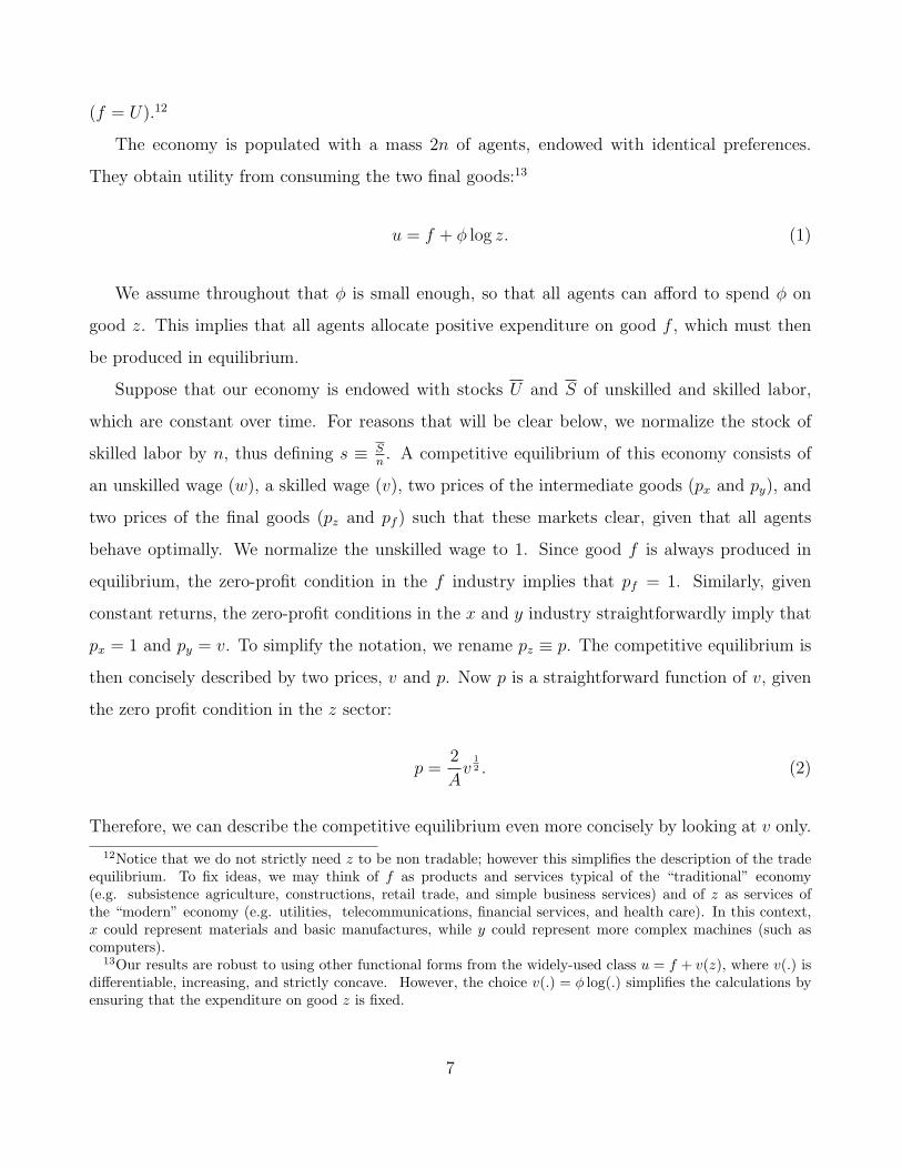
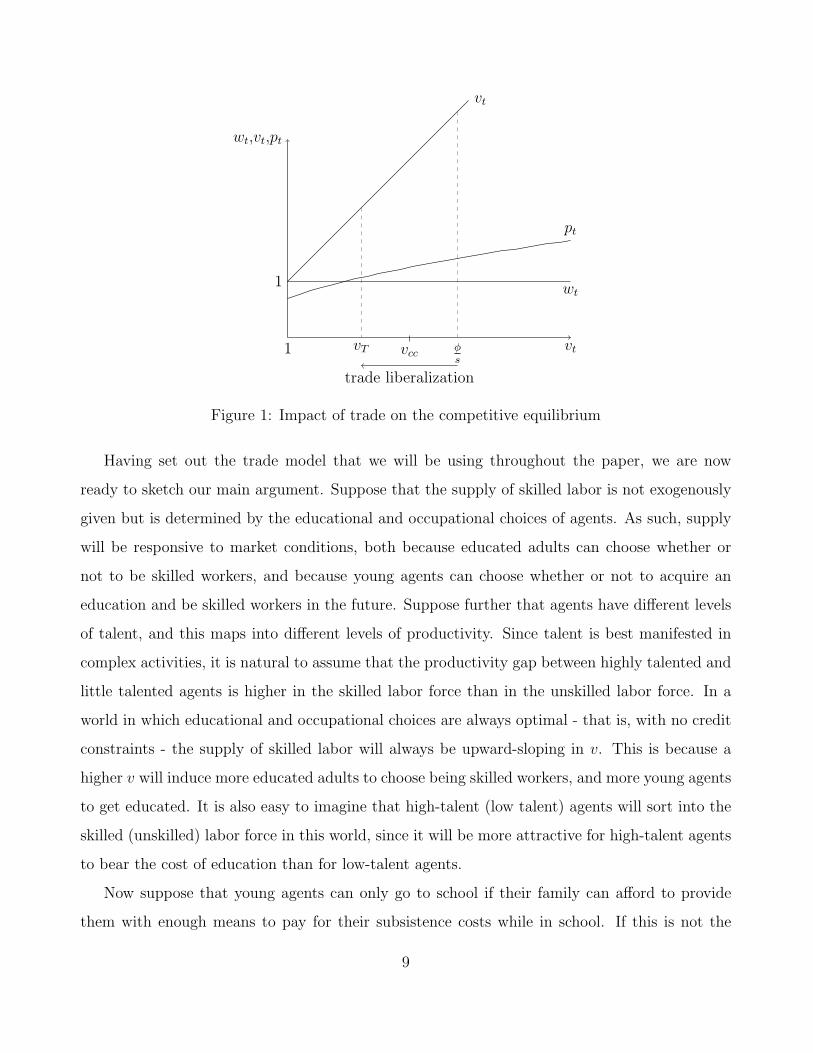
in H (vT < vT−1 = φs). Figure 1 describes the impact of trade on the competitive equilibrium.

The figure represents equilibrium wages and final good prices as functions of the equilibrium

skilled wage. As we have just seen, trade liberalization at time T decreases the skilled wage from

φs

to some lower value vT .

Clearly, trade has two consequences for the structure of wages in the domestic economy. First,

it decreases the skill premium, which we define in this paper as the ratio of average, observed

skilled to unskilled wages (here simply πt ≡ vt

wt= vt). Second, it decreases the purchasing power

of skilled wages in terms of the final goods, while it increases the purchasing power of unskilled

wage.15 This is, of course, nothing but an application of the standard Stolper-Samuelson theorem.

14We also assume W to be at steady state, so that world prices remain constant over time.15Notice that both v

p and vpz

= v fall following trade liberalization, while wp = 1

p increases and wpz

remainsconstant at 1.

8

1 vt

1

wt,vt,pt

pt

wt

vt

φs

vT vcc

trade liberalization

Figure 1: Impact of trade on the competitive equilibrium

Having set out the trade model that we will be using throughout the paper, we are now

ready to sketch our main argument. Suppose that the supply of skilled labor is not exogenously

given but is determined by the educational and occupational choices of agents. As such, supply

will be responsive to market conditions, both because educated adults can choose whether or

not to be skilled workers, and because young agents can choose whether or not to acquire an

education and be skilled workers in the future. Suppose further that agents have different levels

of talent, and this maps into different levels of productivity. Since talent is best manifested in

complex activities, it is natural to assume that the productivity gap between highly talented and

little talented agents is higher in the skilled labor force than in the unskilled labor force. In a

world in which educational and occupational choices are always optimal - that is, with no credit

constraints - the supply of skilled labor will always be upward-sloping in v. This is because a

higher v will induce more educated adults to choose being skilled workers, and more young agents

to get educated. It is also easy to imagine that high-talent (low talent) agents will sort into the

skilled (unskilled) labor force in this world, since it will be more attractive for high-talent agents

to bear the cost of education than for low-talent agents.

Now suppose that young agents can only go to school if their family can afford to provide

them with enough means to pay for their subsistence costs while in school. If this is not the

9

case, young agents must work as unskilled workers instead of going to school, thus losing the

chance to be skilled workers in their adulthood. Under these circumstances, it is conceivable

that v may be very high, and yet the supply of skilled labor may be very low (explaining why v

is high in the first place). The intuition for this is provided by Figure 1. When v is very high,

the cost of subsistence - which in our setting is fully captured by p16 - is high for families of

unskilled workers, while it is low for families of skilled workers. Thus, there will be a threshold

vcc such that if v > vcc, it is only the families of skilled workers who can pay for their children’s

subsistence while in school. For any initially low stock of s, there will then be an equilibrium in

which v is very high, and the supply of skilled workers is very low. The key thing is to notice

that since v is very high in these equilibria, children of skilled workers will have strong incentives

to go to school even if they are low-talent. The existence of low-talent workers in the skilled

labor force will then drag down the observable, average skilled wage in the economy.

What happens if country H is opened up to trade with W , along the lines described above?

Just as before, trade must decrease v: thus, the skill premium within any given pair of skilled-

unskilled workers must also decrease, along standard Stolper-Samueson lines. But what does

trade do the relative composition of the skilled/unskilled labor force? Here, there are two effects.

On the one hand, because v is now lower, some low-talent educated adults who have an education

only because they were children of skilled workers in a high-v, pre-trade economy, may want to

drop out of the skilled labor force. On the other hand, some high-talent children of unskilled

workers who would have been excluded from school in the pre-trade economy may now be able

to go to school. This is because trade has increased the purchasing power of families of unskilled

workers, and thus their capacity to pay for their children’s subsistence while in school. Both

effects push for a net transfer of talent away from the unskilled labor force and into the skilled

labor force. When we look at the observed, average skilled premium in the economy, this talent

re-allocation will make sure that trade always has a less negative effect on the skill premium than

in a world with homogenous agents and no credit constraints. In fact, we show in the next section

that trade may even have a positive effect on the skill premium. Thus, talent heterogeneity and

credit constraints make it possible that for an economy experiencing a fall in the relative price

16Recall that the price of the other final good is normalized at 1.

10

of skill-intensive goods, the predictions of the Stolper-Samuelson theorem can be reversed. We

now move to illustrating this result more formally.

3 The Model

In this section, we begin by combining the simple trade model developed in the previous section

with a model of overlapping generations (section 3.1), where the decision to become skilled is

endogenous (section 3.2). After summarizing the sequence of events in each period (section 3.3),

we solve for the autarchic steady state of this combined model (section 3.4). Our main results

are contained in section 3.5, where we study the impact of trade liberalization on the observed

skill premium in this economy.

3.1 Demographics

At any given time t, the economy is populated by two overlapping generations of agents, who

live for two periods. “Generation t− 1” is made up of agents who were born in period t− 1, and

are adult in period t. There is a mass n of such agents. “Generation t” is made up of children of

generation t− 1. They are born at the beginning of period t, and are young in this period. Since

each adult agent gives birth exactly to one child, there is a mass n of young agents in period t.

Thus, the total mass of agents in this period is 2n.

We still use the utility function in (1) to describe how agents obtain utility from the con-

sumption of final goods, but enrich the structure of agents’ preferences in two important ways.

First, all agents face a “survival constraint”, in the sense that if the agent’s utility falls below

a threshold u in any of her two periods of life, this agent dies of starvation (and gets utility

−∞). Second, adult agents also care about the gift (in terms of utility) that they give to their

11

children.17 We represent the agent’s inter-temporal optimization problem as follows:

max uit,t + 2(bit)12 (uit,t+1)

12

s.t. uit,t, uit,t+1 ≥ u

where uit,s = f it,s +φ log zit,s represents the utility obtained by agent i from generation t in period

s, and bit the gift (in terms of utility) given by agent i in generation t.

Notice that, as long as φ is small, the above optimization problem has two very convenient

properties. First, since all agents allocate expenditure φ to the consumption of z, the competitive

equilibrium is identical to the one derived in the previous section. Second, in both periods the

marginal utility of income is constant and equal to 1 when income is more than sufficient to

achieve the subsistence level of utility; it is, instead, infinitely high when income is just sufficient

to achieve this level.18 As we will illustrate in section, 3.2.2, this formulation allows us to

introduce credit constraints in a very analytically tractable way.

Finally, we assume that goods are perishable, and that there are no financial markets. Thus,

income cannot be transferred across periods.

3.2 Schooling

All agents are endowed with one unit of time in each period, and are born unskilled. In their

first period of life, they can choose whether to use their time to be an unskilled worker, or to

go to school. If they work, they can only be an unskilled worker in their second period. If

they go to school, on the contrary, they become “educated” and acquire the option of being a

skilled worker in the second period. Educated parents retain the option to be unskilled workers

in the second period. Thus, there may be three distinct groups of parents in any period t:

non educated parents, educated parents who are skilled workers, and educated parents who are

17Transfers from adult agents to their offspring are often interpreted as bequests in the literature. In oursetting, the transfers occur while the adult agents are still alive and therefore, gift seems like a more appropriateterm.

18A low φ - that is, a low optimal expense on z - ensures that the marginal utility of income is 1 in the firstperiod. The functional form for second-period utility ensures that the marginal utility of income is constant andequal to 1 in the second period as well (see Appendix B for more details). To allow for more general functionalforms would greatly complicate the algebra, without changing the logic of the argument.

12

unskilled workers.

Agents differ in their level of talent, Θ. For simplicity, talent can take only two values,

Θ = 1 and Θ = θ > 1 . We will refer to agents with these talent levels as “untalented” or “low-

talent” and “talented” or “high-talent”, respectively. We assume that talent is not inherited,

but distributed randomly across the population with a probability of observing a talented agent

being equal to β. Thus, each generation has a mass βn of talented agents and a mass (1− β)n

of non-talented agents, and the average talent in the population is:

θ ≡ βθ + 1− β.

While all agents are equally productive when they work as unskilled workers, there is a one-

to-one mapping between an agent’s level of talent and her productivity as a skilled worker. In

other words, a non-talented worker can only contribute 1 efficiency unit of skilled labor, while a

talented worker can contribute θ units. This maps into a higher wage awarded by a competitive

skilled labor market to talented agents (who receive θv) compared to non-talented agents (who

receive v). In what follows we continue to refer to v as the skilled wage, but it should be borne in

mind that what it really indicates is the skilled wage of non-talented agents, or the skilled wage

per efficiency unit of labor.

3.2.1 Participation constraints

We assume that going to school is free, as would be the case of a country where education is fully

subsidized by the government.19 Despite being free, however, going to school comes at the cost of

lost unskilled wages in the agent’s first period of life. When choosing whether to go to school or

not, agents compare this cost to the difference in wages that they can expect to receive working

as skilled workers in their second period of life. Since agents with different levels of talent can

expect to receive different skilled wages, they will also have different participation constraints.

In particular, denoting by vet+1 the skilled wage expected by period t’s young agents for period

t+ 1, an agent of talent Θi goes to school if and only if Θivet+1 − 1 > 1. This gives the following

19This is only a simplifying assumption; see section 3.2.2 for further discussion of this point.

13

participation constraints for talented and non talented agents:

vet+1θ > 2 (4)

vet+1 > 2. (5)

Notice that it is always ex-post optimal for an educated agent to be a skilled worker in period

t+ 1, provided that her expectations in period t were correct.20 Intuitively, the cost of education

is sunk in period t + 1, while the agent’s productivity is unchanged. Rational initial decisions

must then be optimal, unless external conditions have changed.

3.2.2 Credit constraints

Under the assumption that credit markets do not exist, we now move to consider how the school-

ing decisions of agents are driven not only by income maximization (as described in equations 4

and 5), but also by parental wealth. While school is free of charge, agents can only afford to go

to school if the gift that they receive from their parents is high enough to cover their subsistence

expense while in school. If this is not the case, agents must join the unskilled labor force and

pay for their own subsistence expense, or else die of starvation. Thus, the distribution of gifts

determines who can and cannot go to school from the set of young agents. We will refer to the

latter group as credit constrained young agents.

The assumption that wage income is harder to give up for poor young agents than for rich

ones is broadly consistent with the way in which educational credit constraints are modeled

in the literature.21 For example, Ranjan (2003) assumes a continuously decreasing marginal

utility of income, which, coupled with the inability to borrow from financial markets, implies

that the participation constraint of the poor is less likely to be satisfied than that of the rich.

Our innovation is that we model the marginal utility of income as decreasing at a single point

20This is clear from the fact that the ex-post participation constraints of the two types are vt+1θ > 1 andvt+1 > 1, which are always satisfied if (4) and (5) hold and vt+1 = vet+1.

21An alternative formulation is that agents must pay a fee to go school; in the literature on trade with edu-cational credit constraints, such a fee is then typically modeled as increasing in the skilled wage (e.g. Cartiglia,1997). While we believe that our formulation is more realistic, we stress that none of our results hinge on thespecific way in which we introduce educational credit constraints.

14

of the income distribution - infinite at the level of income that is needed to pay for subsistence,

constant and equal to 1 thereafter. The advantage of this formulation is that it allow us to model

credit constraints separately from participation constraints, keeping the latter linear.22 While

fully preserving the logic of the mechanism, this allows us to simplify the algebra a great deal.

This way of modeling educational credit constraints is in line with abundant empirical evidence

suggesting that a major force keeping the poor out of school is the high opportunity cost from

lost labor opportunities, given their proximity to the subsistence level of income.23

We now proceed to study the shape of the distribution of gifts, and its impact on the schooling

decisions of agents. In any period t, parents can fall into three income brackets: unskilled workers

(income 1), skilled but non-talented workers (income v), or skilled and talented workers (income

vθ). Because educated parents are free to choose whether to work in the skilled or unskilled labor

force, income in the two latter brackets cannot fall below 1 in equilibrium. Thus, the minimum

gift that is transferred in period t is 12, which is what the offspring of unskilled workers receive.

These agents are the first to become credit constrained when the cost of achieving the sub-

sistence level of utility increases. Specifically, for these agents not to be credit constrained in

period t the following condition must hold:

e(u, pt) ≤1

2(6)

where e(u, pt) is the expenditure function valued at the subsistence level of utility and at current

prices. When condition (6) does not hold, the offspring of unskilled workers must work as

unskilled workers in their first period of life, or else die of starvation.

22What we call a “credit constraint” is, strictly speaking, a further participation constraint, that young agentsface before those in (4) and (5). Young agents first assess whether it makes sense for them to go to school, giventhat this may give them the infinitely negative payoff associated with starvation. If they decide that it does -that is, if starvation is not an issue - they then assess whether it makes sense to give up a career as an unskilledworker, to work as skilled in their adulthood. Of course, the first participation constraint is only there becauseagents cannot borrow their way out of starvation, which is our rationale for calling it a credit constraint.

23For example, Cartwright (1999) argues that Colombian boys become increasingly likely to drop out of schoolas they grow older, as their opportunity cost from lost labor opportunities increases. He also finds that a 1%increase in household expenditure map into a .11% (.19%) lower probability of work for a rural (urban) child.Cartwright and Patrinos (1999) find similar results for urban Bolivia. In both cases, there is also evidence thatthe existence of household assets decrease the probability of work, suggesting the importance of credit constraintsfor schooling decisions.

15

Importantly, we can focus on that part of the expenditure function around the threshold

value 12: since φ < 1

2by assumption, and φ is the optimal expenditure on good z, the relevant

part of the expenditure function is the one at which consumption of good z is at its optimum

value ( φpt

). Since the utility from consuming this amount of z is φ log φpt

, the relevant part of the

expenditure function is simply:

e(u, pt) = φ+ u− φ logφ

pt.

That is, the cost of achieving utility u is given by the cost of the optimal consumption of z

(φ), augmented by the cost of increasing utility from φ log φpt

to u through consumption of f . We

can now re-write the expenditure function in terms of vt by plugging in (2):

e[u, pt(vt)] = F (u,A) +φ

2log vt (7)

where F (u,A) ≡ φ+ u− φ log φA2

. Not surprisingly, the cost of subsistence is always strictly

increasing in v - a measure of the scarcity of skilled labor in the economy, and thus the cost of

producing z. Moreover, the cost of subsistence takes value in the open interval (0,∞) for vt ∈

(0,∞).24 Plugging (7) into (6), we obtain:

vt ≤ exp

{1− 2F (u,A)

φ

}≡ vcc. (8)

Inequality (8) defines a threshold for the current skilled wage that is critical in determining

whether the offspring of unskilled agents are credit constrained or not. In particular, if vt ≤ vcc

the offspring of unskilled agents are not credit constrained, while they are if vt > vcc. Intuitively,

an increase in vt (that is, a more scarce skilled labor force) is associated with a high cost of

production in the z sector, a higher pt, and a higher subsistence cost (recall that e(u, p) is

increasing in p). For the offspring of unskilled workers, this increase in subsistence cost is not

24When the cost of subsistence is above φ, (7) is the relevant expression for it. Clearly, this is strictly increasingin vt, and converges to∞ as vt converges to∞. When the cost of subsistence falls below φ, the relevant expression

becomes e[u, pt(vt))] = 2v12t

A exp(uφ

), since compensated demand for f and z is, respectively, zero and exp

(uφ

).

This is also strictly increasing in vt, and converges to 0 as vt converges to zero.

16

matched by an increase in gifts, which is only linked to the unskilled wage. Thus, a high enough vt

implies that the offspring of unskilled agents must work as unskilled workers in the first period of

their life to meet their subsistence needs. Not surprisingly, the threshold vcc is always increasing

in A, the total factor productivity in the z sector. Intuitively, a more productive economy makes

the cost of subsistence smaller for any existing stock of skilled labor, thus reducing the probability

that the offspring of unskilled workers are credit constrained. In fact, we can always set A large

enough so that vt ≤ vcc, and credit constraints are not an issue for this group of agents.

We have established that a high skilled wage may be bad news for the offspring of unskilled

workers, in that it may force them to remain in the unskilled labor force as well. But how about

the credit constraints of the offspring of skilled workers? As we have already noticed, these

agents must be at least as wealthy as the offspring of unskilled workers in equilibrium. Thus, if

the latter are not credit constrained in equilibrium (it is vt ≤ vcc), the offspring of skilled workers

cannot be. If the offspring of unskilled workers are credit constrained (it is vt > vcc), we show

in Appendix A that a sufficient condition for the offspring of skilled workers not to be credit

constrained is that vcc > 1. Intuitively, a high enough vt must be good news for the offspring of

skilled workers: this is because the gift that these agents receive is linear in vt, while the cost of

subsistence is concave. It must then be the case that the former overtakes the latter for vt higher

than a certain threshold. The condition vcc > 1 makes sure that this threshold is lower than vcc,

implying that the offspring of skilled workers will never be credit constrained for vt > vcc. Since

we will anyway want to restrict our attention to cases in which vcc is high (and higher than 1,

see Section 3.4), we can safely conclude that the offspring of skilled workers will never be credit

constrained in equilibrium.

In the rest of the paper, we will study how a trade-induced decrease in vt may lead to a

relaxation in the credit constraints of the offspring of unskilled workers. In this context, the

results derived above may be seen as a corollary of the classic Stolper-Samuelson theorem. This

states that a trade-induced rise in the relative price of a good raises the real return of the factor

used intensively in the production of that good, and lowers the real return of the other factor, in

terms of both goods in the economy. In our model, trade will increase the price of good x, thus

increasing the real return to unskilled labor in terms of both x and y (and thus z). This will

17

then result into a lower cost of subsistence for the offspring of unskilled workers, relaxing their

credit constraints.

Notice that the existence of a subsistence level of utility must put a constraint on the minimum

endowment of productive factors in an economy. In this model with human capital accumulation,

this requires ruling out that there are too few educated agents at any point in time. To see this,

notice that if e(u, p) > 1, unskilled workers are never able to reach the subsistence level of utility

- not even if they do not give any gifts to their offspring. Thus, all unskilled workers would pass

away in this case, and the economy would collapse. To avoid this, we require e(u, pt) ≤ 1 at all

t. Using (7), this can be equivalently written as:

vt ≤ exp

{2− 2F (u,A)

φ

}≡ v.

Notice that, since v = vcc exp{

1φ

}, it is always the case that v > vcc. Furthermore, being a

linear function of vcc, v depends on A just as vcc does. In what follows, we will only consider

the case in which the economy never collapses, or in which vt < v in all periods. This requires

imposing some restrictions on initial conditions, as vt < v will then emerge naturally from the

agents’ schooling decisions under the model’s assumptions.

3.3 Timing and equilibrium concepts

The following events take place in each period t:

t.1 Generation t is born from parents of generation t− 1;

t.2 Educated parents decide whether to be skilled or unskilled workers. At the same time,

individuals of generation t decide whether to join the unskilled labor force or go to school.

t.3 Production takes place; all markets clear.

t.4 Gifts are made, consumption takes place.

t.5 Parents pass away.

18

Just as in section 2, a competitive equilibrium at time t is defined as a vector of prices such

that all markets clear, given that all agents behave optimally and a positive amount of good f

is produced. It is important to notice that, with endogenous schooling and working decisions,

this definition includes two additional requirements on the optimal behavior of agents. First, the

schooling decisions of young agents in t− 1 (and thus the supply of educated parents in t) must

be optimal given the prices that are realized in t. We consider this to be a feature of period t’s

equilibrium (rather than period t − 1’s) because schooling decisions in period t − 1 only affect

prices in period t.25 Second, the working decisions of educated parents at time t (and thus the

supply of skilled labor in t) must also be optimal given the prices in period t.

While the competitive equilibrium in period t is never affected by the equilibrium in period

t + 1, it may well be affected by the competitive equilibrium in period t− 1. To illustrate this,

it is useful to consider a specific parametric specification where this “path dependency” does

not take place, and then contrast it with a more general specification of the model. Suppose

that u → −∞, so that e(u, pt−1) → 0. In this case, no agents is ever credit constrained, and

schooling decisions at time t− 1 are only affected by expected prices at time t: in other words,

the equilibrium at time t is not affected by conditions prevailing at any previous period. Suppose

now that e(u, pt−1) > 0. In this case, the children of unskilled agents will be credit constrained

for vt−1 > vcc. Thus schooling decisions at time t− 1 (a feature of the equilibrium at time t) will

be affected by the level of prices at time t− 1 (a feature of the equilibrium at time t− 1).

In what follows, we will be interested both in the model’s transitional dynamics - that is, the

evolution of the competitive equilibrium over time - and its steady state. The latter is achieved

at time t if the competitive equilibrium realized at that time is identical to those realized at

times t+s, were s = 1, ...,∞. That is, all generations make the same schooling and occupational

choices in steady state, and prices remain constant over time. Notice that the model only displays

a transitional dynamics if there is path dependency (and thus credit constraints): clearly, if the

competitive equilibrium at any given point in time does not depend on earlier conditions, the

economy must be in a steady state.

25This important feature of the model relies on the fact that good f is always produced, and the relative wagedoes not depend on the amount of unskilled workers in the economy.

19

Having defined our equilibrium concept, we now move to describing the competitive equilib-

rium of country H.

3.4 Autarchy equilibrium

We begin by making two assumptions on the distribution of talent and on the level of credit

constraints in the economy:

Assumption 1. β ∈(φ2θ, φ

2

)Assumption 2. vcc > 2.

Assumption 1 requires that the number of talented agents in the population be “intermedi-

ate”, where the lower bound of the allowed range is decreasing in the ratio of the high level of

talent to the low level of talent (θ). As will be clear below, this assumption merely simplifies the

description of the equilibrium, given the discreteness of the distribution of talent. Assumption

2 requires that productivity in the economy be high enough, so that the threshold above which

the offspring of unskilled agents are credit constrained is not too small. This assumption is

necessary to make sure that there exists an equilibrium in which talented agents are not credit

constrained. This is the interesting case for us, as it is the one in which trade may lead to a

better allocation of talent in H, thus affecting the skill premium in a non-standard way. Notice

also that Assumption 2 implies vcc > 1, and so that we are safe to assume that the offspring of

skilled workers are never credit constrained in equilibrium (see section 3.2.2).

We are now ready to describe the autarchy steady state of country H. For conciseness, we

only report the schooling decisions of agents and the skilled wage in steady state:

20

Proposition 1. From any (feasible) initial stock of educated parents at t = 1, the economy

converges to a unique steady state no later than t = 3. Depending on the initial stock, this can

be:

• A “good steady state” in which v = φβθ

, and all and only the talented agents go to school.

• One from a continuum of “bad steady states” in which v ∈ (vcc, v] > φβθ

, and all and only

the offspring of skilled workers go to school.

Proof. See Appendix C.

Proposition 1 argues that from any initial stock of educated parents (which cannot be too

small, or else the economy would implode due to starvation) the economy quickly converges to

a steady state, and that there is a one-to-one mapping between the initial stock and the type

of steady state that the economy converges to. There are two, quite distinct types of steady

states. On the one hand, there is a unique “good” steady state in which all and only the talented

agents go to school, and the skilled wage is relatively low. This is a steady state in which credit

constraints are not binding, and talent is efficiently allocated to the skilled labor force. On the

other hand, there is a whole class of “bad” long-run steady states in which all and only the

offspring of skilled workers go to school, and the skilled wage is relatively high. In these steady

states credit constraints are binding for a fraction of the population, and the allocation of talent

to the skilled labor force is inefficient. Intuitively, the offspring of unskilled workers cannot afford

to go to school if v > vcc, while the offspring of skilled workers can. This implies that it will be

only the offspring of skilled workers who go to school for v > vcc. Furthermore, since vcc > 2, it

must be the case that all of them to go to school, creating a steady state in which the skilled

labor force self-perpetuates itself over time.26 The only constraint on this class of steady states

26Notice that we could relax Assumption 2 to vcc > φβθ . This would imply a slightly more complicated

transitional dynamics for the case in which v1 ∈ (vcc, 2], but not change the result that the economy convergesto one of the “bad” steady states when v1 > vcc.

21

is that v cannot be greater than v, or the economy would collapse.27

Figure 2 illustrates convergence to the steady state from any (feasible) stock of educated

parents at t = 1, and thus any (feasible) v1. Because the working decisions of young agents do

not affect the competitive equilibrium in period 1, we can treat v1 as exogenous to the schooling

decisions of generation 1. The left-hand panel represents the case in which v1 ≤ vcc. In this case,

no one is credit constrained in period 1. Because of rational expectations and certainty, this

implies that the skilled labor supply at t = 2 will include all of the talented agents of generation

1 if v2 >2θ, and all of generation 1 if v2 > 2. Under Assumption 1, demand and supply meet in

the first vertical portion of the supply schedule. Thus, the competitive equilibrium in period 2 is

such that all and only the talented agents go to school in period 1, and v2 = φβθ

. Because φβθ< vcc

by Assumption 2, this is also a steady state (the “good” steady state described in Proposition

1).

v

v

2vcc

φβθ

2θ

βθ θs

sd

ss2

Good SS

Case 1: v1 ≤ vcc

v

v

2vcc

φβθ

2θ

βθ θs

sd

ss2 ss3(ss2)′ = (ss3)

′

Good SS

Bad SS

Case 2: v1 > vcc

Figure 2: Autarchy steady states

The right-hand panel represents the case in which v1 > vcc. In this case, the offspring of

skilled workers are the only ones who can go to school in period 1. The supply of skilled labor

in period 2 is then everywhere lower than in the previous case, reflecting the fact that schools

can only attract students from a portion of the population. There are then two distinct cases. If

27Notice that the cost of subsistence ranges from 12 to 1 as v ranges from vcc to v. For these high values of the

cost of subsistence, unskilled parents live as a gift less than a share 12 of their second period’s income to their

offspring. This does not matter for our result, however, as these offspring would have been credit constrainedanyway for v > vcc.

22

educated parents in period 1 are not too few in number, the supply of skilled labor in period 2

is not too low (ss2 schedule), and v2 ≤ vcc. Because credit constraints are not binding in period

2, supply in period 3 (ss3 schedule) is identical to supply in the left-hand panel, and the economy

converges to the good steady state in period 3. If instead there are very few educated parents

and v2 > vcc ((ss2)′ schedule), credit constraints are still binding in period 2, and the offspring

of skilled workers are again the only ones that can go to school. Because v2 > 2, the number of

skilled workers in t = 2 must be the same as in t = 1. It follows that the supply of skilled labor

in t = 3 ((ss3)′ schedule) will be identical to supply in t = 2, and a “bad” steady state is reached.

Having found all the possible steady states at which H can be in autarchy, we next move

to consider how the steady state of this country may be affected by opening up to trade with a

foreign country.

3.5 Trade equilibrium

We now study what happens if, at time T , H opens up to trade with the external world (W ).

As explained in section 2, we assume that W is relatively large, and is in steady state. This

implies that the world prices of x and y are exogenous and constant over time, and H’s prices

are equalized to them following trade liberalization. We also assume that W ’s relative price of

y is initially lower than H’s, so that W ’s skilled wage per efficiency unit of labor, v∗, is lower

than v before trade liberalization.28 Clearly, this is equivalent to assuming that W is more

skill-abundant than H before trade liberalization.

Since we are interested in the impact of trade on a credit constrained economy, we assume

that H starts out at one of the bad steady states described in Proposition 1. There are then two

kinds of reasons why W may be initially more skill-abundant than H. On the one hand, this

may be due purely to weaker credit constraints in W than in H, so that a higher proportion of

people (and/or more talented people) go to school in W than in F . Alternatively, W may be

more skill-abundant due to a variety of structural factors - such as a more skill-biased technology

or a better educational system - that make the effective supply of skilled labor higher in W , for

any given level of credit constraints. While in both cases W has an initial comparative advantage

28Since trade equalizes salaries, we can normalize the skilled wage to 1 both in H and in W .

23

in the production of y, in the first case this may be dissipated over time, or even reversed. This

is because trade may move H to an equilibrium with weaker credit constraints, thus making it

as skill-abundant as W or even more. For simplicity, we assume that there are some structural

factors underpinning W ’s comparative advantage in the production of y, such that this does

not fully dissipate if H converges to its “good” equilibrium. The existence of this “structural”

comparative advantage of W requires that we assume v∗ < φβθ

from now on.29

Before investigating the impact of trade on schooling and working decisions, we must specify

the timing of trade liberalization and its relation to agents’ expectations. A full-fledged analysis

of trade liberalization in a model with rational expectations would require us to specify to what

extent trade liberalization at time T is foreseen by agents in previous periods. This is important

because, for example, the possibility of trade liberalization affects the expected skilled wage at

time T , thus influencing the schooling decisions at time T − 1. While making the analysis more

coherent, to account for the expectation of trade liberalization would greatly complicate the

model, as it would link the autarchy equilibria of the two countries to each other even before

trade is opened. At the same time, this extension would not undermine the logic of our argument

unless trade liberalization is fully foreseen - a case that we consider unlikely. For these reasons,

we choose to model trade liberalization as a fully unexpected event in period T . To facilitate the

intuition, this simple model can be thought of as substantially equivalent to one in which trade is

opened in period T , and the probability perceived beforehand that this would happen was very

low.

To introduce trade in our framework, we enrich the timing at period T (and at period T

only) by adding the following event:

T.0 Trade is opened (to remain open forever after).

29A natural way to obtain this pattern of comparative advantage is to assume that W is itself at the goodequilibrium, but that its technology is biased in favor of skilled occupations (e.g. x∗ = U and y∗ = A∗S∗, withA∗ > 1). Total supply of skilled labor would then be Aβθ > βθ, leading to v∗ < φ

βθ . Notice that it is only tosimplify the exposition that we assume this structural comparative advantage of W . We could allow for W ’scomparative advantage to dissipate fully, or be reversed, as H converges to its good equilibrium, and all of ourresults would still hold for some value of the parameters. For an example where W ’s comparative advantage fullydissipates over time, the interested reader is referred to the working paper version of the paper (Bonfatti andGhatak, 2011).

24

That is, trade is opened immediately before generation T is born in T.1, and remains open

forever after. At time T.2, educated parents decide whether to join the skilled labor force or not.

As in autarchy, this choice and the prices that form in period T.3 must constitute a competitive

equilibrium. Because conditions have unexpectedly changed, however, schooling decisions in

period T − 1 need not be optimal anymore. In particular, it may well be the case that some

of the educated parents decide to stay out of the skilled labor force, as trade has depressed

the skilled wage to a level well below what they expected when they decided to go to school.

This misalignment between expected and real prices lasts for one period only. Because there

is no uncertainty after period T - trade remains forever open, and this is common knowledge -

generation T ’s schooling decisions must correctly reflect prices as they will form under free trade

in period T + 1. Notice that trade affects the schooling decisions of generation T in two ways.

It may affect their participation constraints, by changing the level of the skilled wage in T + 1;

and it may affect their credit constraints, by changing the level of the skilled wage in T .

Our first result is presented in the following proposition:

Proposition 2. Opening up to W in period T shifts H to a new steady state in period T+1, where

v = v∗, no one is credit constrained, and only talented agents go to school. If W ’s comparative

advantage in the skill-intensive sector is not too strong, this is the good equilibrium where all of

the talented agents go to school. At all t ≥ T , H is a net importer of y.

Proof. See Appendix C.

Proposition 2 suggests that if H is at a bad steady state and it opens up to a relatively skill-

abundant world, trade may trigger a mechanism that shifts H to the good steady state within

a generation. The intuition for this result is straightforward. Because W has a comparative

advantage in y, trade reduces the price of this good in H. This reduces the reward to skilled

labor, the factor in which production of y is relatively intensive. This reduction is assumed to be

large enough to take the skilled wage below the threshold vcc. But for vT < vcc the offspring of

unskilled workers are not credit constrained anymore, and all of generation T ’s talented agents

25

can choose to go to school in period T . Furthermore, while the (expected) skilled wage has

fallen relative to its pre-trade level, it may still be high enough to motivate at least some of

these agents to go to school. Of course, this is only possible because credit constraints, and not

participation constraints, prevented these agents from joining the skilled labor force in autarchy.

On the contrary, the non-talented offspring of skilled workers - who would have gone to school

had the (expected) skilled wage remained at its pre-trade level - are now better off opting out of

the schooling system. It follows that all and only the talented agents go to school after trade is

opened, and the economy moves to the good steady state in period T + 1.30

The result that trade may move the unskilled labor-abundant country from a low human

capital equilibrium to a high human capital equilibrium is very similar to the results found

by Ranjan (2003). More generally, that trade may lead to an increase in school enrollment

among the offspring of unskilled workers is a key result in the literature on trade with credit

market frictions and trade, beginning with Cartiglia (1997). These results are consistent with a

few recent empirical studies on the impact of trade liberalization on child labor. For example,

Edmonds and Pavcnik (2005) find that a trade-induced increase in the price of rice in Vietnam

was associated with a decrease in child labor in households that were net sellers of rice, but

with an increase in households that were net buyers. Similarly, Kis-Katos and Sparrow (2010)

exploits variation in the degree of trade liberalization across Indonesian districts to argue that

trade liberalization is associated with a decrease in child labor, and that this effect is strongest

for children from low-skill backgrounds.

We now turn to the main focus of the paper, which is to consider the consequences of trade

for the skill premium. Notice that the skill premium in any period t is now given by:

πt ≡ (θS)tvt

where (θS)t denotes the average talent of members of H’s skilled labor force in period t. Following

the empirical literature, we define the skill premium as the ratio of the average wage of members

30The spirit of the model would be preserved if firing costs prevented (or slowed down) the reallocation of laborfrom sector x to sector y, because the average unskilled wage would still increase relative to the average skilledwage (see also footnote 21).

26

of the skilled labor force by the average wage of the members of the unskilled labor force (which

is always 1 in equilibrium in our model), not controlling for the unobservable talent of workers.

We begin by considering the impact of trade on the skill premium in steady state, and then we

will comment on its impact during the transitional dynamics.

The long-run effect of trade on the skill premium is described in the following proposition:

Proposition 3. Following trade liberalization in period T , H’s skill premium at all t ≥ T + 1 is

given by:

πt =θ

θ

v∗

vT−1

πT−1.

Proof. From Proposition 2, we know that (θS)t = θ for all t ≥ T + 1, and therefore πt = θv∗.

From Proposition 1, and because we have assumed that H starts out at one of the bad steady

states, we know that (θS)T−1 = θ, and therefore πT−1 = θvT−1. We may then write:

πt = θv∗ =θ

θ

v∗

vT−1

πT−1. (9)

Proposition 3 studies the effect of trade on the skill premium in the new steady state. Since

trade is opened in period T but the new steady state is reached only in period T + 1 (see

Proposition 2), we will also refer to this as the “long-run” impact of trade on the skill premium.

The proposition suggests that the new steady state skill premium in H is the product of its

pre-trade liberalization level and two distinct terms. The first is the ratio of the level of the

skilled wage post-trade liberalization to its level pre-trade liberalization ( v∗

vT−1). Because H is

on the unskilled labor-abundant side of the trade relation, this term must be smaller than 1 in

equilibrium. Thus, the impact of trade on the skill premium as described by the first term is just

as in a standard Stolper-Samuelson world: trade decreases the skill premium in the unskilled

labor-abundant country, because it decreases the skilled wage relative to the unskilled wage.

However, the second term in the product, namely θbθ , introduces an important qualification to

27

this conclusion. The term captures the extent of talent re-allocation following trade liberalization,

or, alternatively, the degree of talent misallocation in H before trade liberalization. Since θ > θ

- trade always improves the allocation of talent to the skilled labor force - this term must be

greater than 1. Thus, the immediate gist of Proposition 3 is that the Stolper-Samuelson effect

on the skill premium is always moderated by the reallocation of talent. In Appendix D we show

that it is possible to have θbθ > v∗

vT−1in our parameter space, i.e., the Stolper-Samuelson effect

may be reversed when the initial degree of talent misallocation in H is large enough.31

We have thus found that in a world with credit constraints that affect the acquisition of

human capital, trade with a large skill-abundant world will have a less negative, and possibly

a positive effect on the steady state skill-premium of a skill-scarce country. The intuition for

this result is straightforward. By increasing the real purchasing power of unskilled workers in

terms of the tradable goods in the economy, trade increases the capacity of the talented offspring

of unskilled workers to pay for their subsistence expenses when going to school. At the same

time, by lowering the skilled wage per efficiency unit of labor, trade discourages the non-talented

offspring of skilled workers to go to school as they would have done in the pre-trade world. These

two forces increase the average talent of those who go to school after trade liberalization, leading

to higher remunerations and possibly to a reversal of the Stolper-Samuelson theorem.

The result that trade liberalization may trigger convergence to a new, high skill-premium

steady state is consistent with evidence documenting an increase in the skill premium for a

protracted period of time (between eight and fifteen years) following trade liberalization. This

evidence has been presented for Chile, Mexico, Argentina, Brazil, Colombia and India (see Gold-

berg and Pavcnik, 2007, pp. 52-53 for a review of the literature).

It is important to notice that the increase in the skill premium after trade liberalization is only

possible if, for a given increase in the school enrollment of talented people, there is a sufficiently

large decrease in the school enrollment of non-talented people. These opposite movements (in and

out of the schooling system) might explain why aggregate school enrollment increased relatively

31In passing, we note that the effect of a given reallocation of talent would be even stronger if productivitydepended on talent in the unskilled labor force as well, as an increase in the average talent of the skilled laborforce would then be accompanied by a decrease in the average talent in the unskilled labor force. This point isgiven further consideration in section 4.

28

little after trade liberalization in Latin America, while the skill premium increased significantly.

This compares with the case of South-East Asia, where trade liberalization was followed by a

much larger increase in aggregate enrollment and by a decrease in the skill premium. This latter

pattern is consistent with the prediction of the Stolper-Samuelson theorem and of our model

for the case in which the movement out of the schooling system is very small relative to the

movement into the schooling system.

We next consider the effect of trade liberalization on the skill premium during the transitional

dynamics, or in the “short run”. This is summarized in the following proposition:

Proposition 4. Following trade liberalization in period T , H’s skill premium in period T is given

by:

πT = Φv∗

vT−1

πT−1

.

where Φ = 1 if v∗ > 1 and Φ = θbθ if v∗ < 1.

Proof. If v∗ > 1, all educated parents opt for staying in the skilled labor force in period T . Thus,

it is (θS)T = (θS)T−1 = θ. It follows that πT = v∗

vT−1πT−1, since πT = θv∗ and πT−1 = θvT−1. If

v∗ < 1, all non talented educated parents opt out of the skilled labor force, and it is (θS)T = θ.

It follows that πT = θbθ v∗

vT−1πT−1, since πT = θv∗ and πT−1 = θvT−1.

Proposition 4 studies the short-run effect of trade on the skill premium in H. In other words,

it studies the transitional dynamics of the skill premium, before this converges to the steady

state value described in Proposition 3.

Just as in the long-run, our model may display non standard predictions for the impact of

trade on H’s skill premium in the short run. Proposition 4 distinguishes between two cases. If

v∗ > 1, the effect of trade on the skill premium is unambiguously negative in the short run (since

29

v∗

vT−1< 1 always holds). Intuitively, the trade-induced decrease in the skilled wage is not too large

in this case, and all educated parents must then remain in the skilled labor force. This implies

that the average talent in the skilled labor force does not change, and the skill premium must then

decrease. Thus, when H opens up to a world that is not too skill-abundant - and consequently,

the price of skill-intensive goods does not fall by too much - the Stolper-Samuelson predictions

are satisfied, since our talent-reallocation channel is effectively shut down. If v∗T−1 < 1, on the

contrary, this channel can be fully at play. In particular, the extent of talent reallocation is as

high as in the long run ( θbθ ). This is for a slightly different reason, however: in the short run, the

initial misallocation of talent is corrected through the exit of the non-talented educated parents

from the skilled labor force.32

Thus, we have shown that trade-induced compositional change may result in an increase in

the skill premium in the unskilled labor-abundant country, both in the short run and in the long

run. In the short run, the downward pressure put by trade on the skilled wage may induce the

least talented of the existing skilled workers to drop out of the skilled labor force, thus increasing

its average quality. When it happens in the short run, this compositional change always extends

to the long run, as only talented young agents find it optimal to go to school after trade has

been opened. Even if it doesn’t happen in the short run, however, this compositional change still

occurs in the long run. This is because non-talented agents are more likely to join the unskilled

labor force when they are young and unskilled, rather than when they are old and already skilled.

It is easy to show that, if H was skill-abundant country, trade liberalization would always

lead to an increase in the skill premium in the short run.33 Thus, our results are consistent with

the fact that trade between unskilled labor-abundant Latin America and various skilled labor-

abundant parts of the world resulted in an increase in the skill premium in both places. Because

it preserves the standard Heckscher-Ohlin structure in which the skilled wage per efficiency unit

of labor decreases in H, our model is also consistent with the finding that skill intensity in

most Latin American industries increased after trade liberalization.34 Finally, our results are

32This outflow of labor from the tradable sectors is consistent with evidence from Brazil suggesting that tradeliberalization induced labor displacement from the formal sector to the informal and self-employment sector (seeMenezes-Filho and Muendler, 2007).

33See for example the working paper version of the paper (Bonfatti and Ghatak, 2011).34Notice, however, that in a two-country world the model would predict a decline in skill-intensity in the North,

30

also compatible with the observation that the skill premium increased homogeneously across

industries in skill-scarce countries, independently of the degree of trade liberalization to which

each industry had been exposed (see Attanasio, Goldberg and Pavcnik, 2004, for the case of

Colombia).

It is important to highlight that our short-term compositional effect may apply to all cohorts

of agents that have already acquired an education at the time of trade liberalization. This

implies that our mechanism is not incompatible with the observation that, in many countries,

trade liberalization has led to an increase in the relative wage of college graduates over a very

short period of time (see, for example, Cragg and Epelbaum, 1996, for the case of Mexico).

Following trade liberalization, low-talent agents who are close to finishing college may still find

it optimal to complete their education. Still, because of the new market conditions triggered by

trade, they may find it hard to find a skilled occupation, and may eventually decide to accept

a less skilled occupation. Thus, at least in principle, the short-run compositional effect of trade

may be at play even for agents that graduate not only before, but also immediately after, trade

liberalization. Similarly, our long-run compositional effect of trade may take no more than a few

years to manifest itself. This depends on how fast pupils close to making a higher education

decision are in reacting to changing market conditions, both on the side of their participation

constraints (for the least talented of them) and on the side of their credit constraints (for the

most talented).35

4 Generalizations

In this section, we generalize the distribution of talent. Suppose that agents may differ in

their productivity both in the skilled and unskilled labor force. In particular, we assume that

which is not in line with the empirical evidence. This suggests that factors other than trade-induced changes infactor prices - for example, a disproportionate increase in productivity in skill-intensive occupations in North -must have been at play.

35In principle, our mechanism may apply to any fixed investment in education that agents have to undertake,including the decision on whether to go to secondary school or not. Notice, however, that our simple educationalmodel does not account for the fact that agents with an intermediate level of skills may drop out of their categorynot only by working as unskilled, but also by deciding to acquire a higher education. Further research is neededto study the compositional impact of trade on the various levels of the skill premium.

31

individual productivity is a random variable drawn from a bivariate distribution(θU , θS

)defined

over [1,∞) × [1,∞). Denote by θ the level of productivity in the skilled labor force, relative

to the productivity in the unskilled labor force(θ ≡ θS

θU

). This is also a random variable, with

probability density function gr (.) and cumulative distribution function Gr (.) defined over [0,∞).

The participation constraint for a young agent with relative productivity θi is now:

vet+1θi > 2.

There is now a potentially infinite number of parental income brackets: this is because,

whether they work as skilled or unskilled, parents can have a potentially infinite number of

different productivity levels. However since the income of unskilled workers cannot fall below 1,

and skilled workers can always work as unskilled workers, the minimum gift that is transferred

in each period must still be greater than 12. The model displays two additional similarities to the

simpler model developed in the previous sections. First, the threshold below which none of the

children of unskilled workers is credit constrained is still defined by vcc (equation 8). Second, the

children of skilled workers are never credit constrained.36 However one important difference is

that in this more general model, some children of highly productive unskilled workers may not

be credit constrained for vt > vcc. The implications of this are discussed further below.

Define vg as the skilled wage at an hypothetical, “good” steady state in which no one is credit

constrained. Just as before, we introduce an assumption to guarantee that such a steady state

exists. To do this, we first need to introduce some notation. Denote by θS(v) the distribution of

productivity in the skilled labor force, when only agents with relative productivity θ ≥ 2v

are in

it. Notice that it is θS(v) = θS for all v > 2 in steady state.37 Denote by θS(v) the average of

θS(v). Then, a sufficient condition for a good steady state to exist is:

Assumption 3. vcc > max{

1, argv

{φv< θ

S(v)[1−Gr

(2v

)]}}.

36Just as in section 3.2.2, they cannot be credit constrained for vt ≤ vcc, since their parents cannot earn lessthan the minimum earned by unskilled workers; nor can they be for vt > vcc, if vcc > 1 (for the formal proof, seeAppendix A).

37For v > 2 in steady state, skilled workers in any period are all the non credit-constrained young agents of theprevious period. Because talent does not depend on parental income, the productivity distribution of this subsetof agent must be identical to that of the general population.

32

Assumption 3 requires that demand for skilled labor at v = vcc be strictly lower than supply,

given that all agents are free to decide whether to go to school or not.38 Just as Assumption 2,

this boils down to a requirement that vcc, or the productivity in the economy, be high enough.

At the same time, to avoid complicated cases in which some children of skilled workers may also

be credit constrained, we continue to assume that vcc must be greater than 1.

With a general distribution of talent, to prove the existence of bad steady states in which v >

vcc is a very complicated task. In the simpler model, any two subsequent periods in which v > vcc

featured an equal number of agents going to school, and with an equal average productivity. This

was because all and only the children of unskilled workers were credit constrained, while, for this

high level of the skilled wage, all children of skilled workers found it optimal to go to school. A

steady state was then achieved in which the skilled labor force self-perpetuated itself through

the generations, displaying a constant average productivity because of the non transmissibility of

talent. In the more general model that we are now looking at, however, the condition v > vcc is

not sufficient to rule out intergenerational mobility, since the children of some highly productive

unskilled workers may not be credit constrained. To find a steady state, we would then need to

derive a set of initial conditions, and conditions on the productivity distribution, such that the

number of such highly productive unskilled workers remains constant over time.39

Because our main interest lies in analyzing the transition from a bad steady state to the good

steady state, we sidestep these complications by simply assuming that bad steady states exist,

and that the home economy may be stuck at one of them before trade liberalization. As H opens

up in period T to a large, relatively skill-abundant world, the skilled wage in H falls from vT−1 to

v∗, to remain at that level at all subsequent periods. Just as before, we allow for the possibility

that v∗ ≤ vg, that is, W ’s comparative advantage in exporting the skill-intensive good may be

due to factors other than the severity of credit constraints in H before trade liberalization. In

38This is sufficient to guarantee that a good steady state exists for the same exact argument used in the proofof Proposition 1. First, demand is continuous and decreasing, while supply is continuous and non-decreasing.Second, demand converges to infinity as v falls to zero, while supply converges to zero. Thus, if no one is creditconstrained in period t, schooling decisions lead to vt+1 = vg ∈ (0, vcc) in period t+ 1. But since no one is creditconstrained for this level of the skilled wage, schooling decisions in period t+ 1 are exactly the same as in periodt, and a steady state is achieved.

39More precisely, for the economy to be at a bad equilibrium, we would need that, in each generation, theincrease in skilled labor due to the children of highly productive unskilled workers that decide to go to schoolperfectly offsets the decrease in skilled labor due to the children of skilled workers who decide not to go to school.

33

fact, we now remain more general as to the severity of such credit constraints. Thus, for a given

vg, H’s relatively high pre-trade skilled wage (vT−1) may now be due to both credit constraints

and other factors (if v∗ < vg < vT−1), only credit constraints (if v∗ = vg < vT−1) or only other

factors (if v∗ < vg = vT−1). To shorten the exposition, we only focus on the impact of trade on

the skill premium in the long-run.

A new version of Proposition 2 can be stated:

Proposition 2a. Opening up to W in period T shifts H to a new steady state in period T + 1,

where v = v∗ and no one is credit constrained. At all t ≥ T , H is a net importer of y.

Proof. See Appendix C.

Before moving on, we introduce a final bit of notation. Denote by θU(v) the distribution of

productivity in the unskilled labor force when only agents with relative productivity θ ≤ 2v

are

in it. Notice that it is θU(∞) = θU . Denote by θU(v) the average of θU(v). With a slight abuse

of notation, denote by θU

(v) the average productivity of agents in the unskilled labor force when

only agents with relative productivity θ > 2v

are in it. Finally, denote by λt the share of young

agents that are credit constrained in period t. Then, the general version of Proposition 3 is:

34

Proposition 3a. Following trade liberalization in T , H’s skill premium at all t ≥ T + 1 is given

by:

πt =θS

(v∗)

θS

(vT−1)

(θU (vT−1)

θU (v∗)+ ψT−1

θU

(vT−1)− θU (vT−1)

θU (v∗)

)v∗

vT−1

πT−1

where:

ψT−1 =λT−1

[1−Gr

(2

vT−1

)]Gr(

2vT−1

)+ λT−1

[1−Gr

(2

vT−1

)] .

Proof. See Appendix C.

Just as in the simpler model, the total impact of trade on the steady state skill premium is

equal to the product of a Stolper-Samuelson term(v∗

vT1

)and a compositional term. The latter,

however, is now significantly more complicated, being itself the product of two distinct terms.

The first term is the result of the fact that trade increases the relative productivity threshold

above which agents work as skilled. This implies that some agents with intermediate relative

productivity - but one that was high enough to join the skilled labor force in the pre-trade world

- now exit the skilled labor force. If these agents’ absolute productivity is low compared to that

of the surviving members of the skilled labor force, this results in an increase in the average

absolute productivity in the skilled labor force. Such an increase always goes in the opposite

direction relative to the Stolper-Samuelson effect (since θS(v∗)

θS(vT−1)

> 1), and may actually reverse

it. This is what happened in our simpler model, where the overall impact of trade on the skill

premium could be positive for a reasonable range of parameters (see Appendix D).

The second term is also the result of the increase in the relative productivity threshold, but

there is also a direct effect of the elimination of credit constraints following trade liberalization.

On the one hand, the term captures the fact that some agents with an intermediate relative

productivity - but one that was too high for them to join the unskilled labor force in the pre-

trade world - now join the unskilled labor force. If these agents’ absolute productivity is high

compared to that of the “old” members of the unskilled labor force, this results in an increase in

the average productivity of the unskilled labor force. Such an increase goes in the same direction

35

as the Stolper-Samuelson effect (since θU

(v∗)

θU

(vT−1)> 1). On the other hand, the term captures the

fact that some agents with a high relative productivity - who could not join the skilled labor

force in the pre-trade world because they were credit constrained - can now leave the unskilled

labor force and join the skilled labor force. While this does not affect the average productivity of

the skilled labor force (which is made larger, but not compositionally different), it does affect the

average productivity of the unskilled labor force. In particular, if the productivity of previously

constrained agents was high, their exit will decrease the average productivity of the unskilled

labor force.

This discussion suggests an important point: trade liberalization is now likely to have a

compositional effect on the skilled and unskilled labor force, even if there are no initial credit

constraints. This is because the impact of trade on the participation constraints is, by itself,

moving agents from one kind of occupation to the other. The fact that these agents are marginal,

rather than average, implies that such a movement may affect the average productivity in the

two kinds of occupations in interesting ways. Of course, initial credit constraints may still have

an important role in the more general model. On the one hand, the more severe are initial credit

constraints, the more the autarchy steady state will have both kinds of misallocation of talent

- agents with a comparative disadvantage in skilled occupations being part of the skilled labor

force, and agents with a comparative advantage in skilled occupations being stuck in the unskilled

labor force. As we shall see momentarily, under reasonable assumptions on the productivity

distribution this will link initial credit constraints to the compositional effect in a way that is

very similar to what we found in our simple model. On the other hand, higher initial credit

constraints imply that trade liberalization is associated with a larger movement from unskilled

to skilled occupations, with potentially important implications for how to interpret the recorded

increase in inequality in welfare terms.

While this discussion confirms that the compositional effect of trade liberalization must be

taken into account when studying the relation between trade and income inequality, our next

goal is to derive meaningful sufficient conditions under which the compositional effect goes in

the opposite direction than the Stolper-Samuelson effect, and can thus be called to account for

some of the increase in inequality that has characterized many developing countries after trade

36

liberalization. Our results are contained in the following two corollaries, that follow immediately

from Proposition 3a:

Corollary 1. With no initial credit constraints, a sufficient condition for the compositional effect

to go in the opposite direction to the Stolper-Samuelson effect is:

θS(k)

θU(k)>θS(k′)

θU(k′)

for any k and k′ such that Gr(k), Gr(k′) ∈ (0, 1), and k < k′.

Corollary 2. Jointly sufficient conditions for a higher level of initial credit constraints to map

into a compositional effect that dominates the Stolper-Samuelson effect are:

• For a given kk′< 1, θ

S(k)

θS(k′)

θU (k′)

θU (k)is increasing in k′;

• θU(k) > θU(k);

where k and k′ are such that Gr(k), Gr(k′) ∈ (0, 1).

Corollary 1 has an intuitive explanation. Suppose that we divide the population in two

groups, the first including only agents with relative productivity above threshold 2k, the second

including all other agents. Clearly, θS(k)

θU (k)is a measure of the average productivity of agents in the

first group who are skilled workers, relative to the average productivity of agents in the second

group who are unskilled workers. Corollary 1 then requires that as the threshold 2k

moves up, the

measure θS(k)

θU (k)also moves up. This condition obtains if, for example, productivity in both types

of occupations increases with θr - say agents with a stronger comparative advantage in skilled

occupations are more talented, and have thus a higher absolute productivity in both occupations

- but being talented matters more for skilled occupations than for unskilled occupations. In this

case, the agents that drop out of the skilled labor force when the threshold moves up increase

the average productivity of the skilled labor force by a lot (as they were very low-productivity

37

compared to other skilled workers), while they increase the average productivity of the unskilled

labor force by little (as their productivity is similar to that of other unskilled workers).40

Corollary 2 suggests two intuitive reasons why higher initial credit constraints are likely to

map into a compositional effect that dominates the Stolper-Samuelson effect. These reflect two

peculiar features of a credit constrained economy. On the one hand, a credit-constrained economy

can admit a very high effective skilled wage, since this is not competed away by massive inflows

into the skilled labor force.41 Many rich agents are then pushed into skilled occupations, despite

having a comparative disadvantage at them. Now if these agents are also less productive at skilled

occupations, and the distribution of θ is skewed towards the bottom, the compositional impact

of these agents moving out of the skilled labor force is likely to be stronger when initial credit

constraints are higher, since there would then be more low-productivity agents leaving the skilled

labor force following trade liberalization.42 On the other hand, a credit constrained economy

features many poor agents working in the unskilled labor force, despite having a comparative

advantage at skilled activities. To the extent that, on average, agents with a stronger comparative

advantage at skilled occupations are also more productive in unskilled occupations (for example,

because they are more talented),43 the negative impact of these agents moving out of the unskilled

labor force will be stronger when credit constraints are initially tighter, since there would then

be more of them.

One final point relates to the impact of trade liberalization on within-group wage inequality

in our framework. In the simple model of section 3, trade liberalization always leads to a

decline in wage inequality in the skilled labor force (while we have assumed away wage inequality

in the unskilled labor force). This result, however, does not necessarily carry through to a

40It is interesting to notice that if talent does not matter for productivity in unskilled activities and θ = θS

has a Pareto distribution, then the compositional effect exactly offsets the Stolper-Samuelson effect. This isbecause the Pareto distribution has a linearly increasing mean residual life, implying that it is always the case

that θS(v∗)

θS(vT−1)

= vT−1v∗ .

41On the contrary, the effective skilled wage does not need to be high in an economy that, say, is skill-scarcebecause of a skill-adverse technology. In such a case, the skilled wage would reflect the low relative productivityof skilled labor.

42The first sufficient condition in Corollary 2 suggests that this must be weighed against the changing impactof this shift on the average productivity in the unskilled labor force.

43In other words, not only does a CEO have a comparative advantage over her secretary in performing her ownCEO job, but she also has an absolute advantage in both her own job and that of her secretary.

38

more general setting. With a general distribution of talent as the one that we have used in

this section, it is in principle possible that trade liberalization leads to an increase in wage

inequality in either groups, or in both. We conjecture that this could happen if dispersion in

relative and absolute productivity was higher at the top-end of the distribution, so that agents

migrating from the skilled to unskilled labor force were relatively homogenous for the former,

and relatively heterogeneous for the latter. While beyond the scope of the current paper, this

extension could help interpret some recent evidence of a rise in within group inequality following

trade liberalization.44

5 Conclusion

In this paper we develop a model of trade liberalization and occupational choice, with capital mar-

ket imperfections. When an economy is unskilled labor-abundant because of credit constraints

that affect the schooling decisions of agents, trade liberalization may have a non-standard effect

on the skill premium. This is for two reasons. First, credit constraints may have allowed a

large number of non-talented agents in the skilled labor force. Having been attracted to the

skilled labor force by a high autarchic skilled wage, these agents may find it optimal to join the

unskilled labor force when trade puts a downward pressure on the skilled wage. Second, credit

constraints may have kept many talented agents out of the skilled labor force. To these agents,

a trade-induced decrease in the cost of subsistence implies a lessening of credit constraints, and

thus a better chance of upward mobility. Both of these effects result in an increase in the average

talent of the skilled labor force, which may lead to an increase in the skill premium despite the

trade-induced decrease in the skilled wage per efficiency unit of labor.

Our results provide a possible explanation for the fact that trade liberalization in unskilled

labor-abundant Latin America led to an increase in the skill premium in both Latin America and

its skill-abundant trade partners. One implication of this is that the increase in the skill premium

in Latin America does not necessarily need to result in a massive increase in income inequality,

as it may be (at least partly) due to a better allocation of talent and more intergenerational

44See, for example, Attanasio et Al. (2004), and Helpman et Al. (2011).

39

mobility.

While reconciling the predictions of the Stolper-Samuelson theorem with the Latin American

experience, our mechanism is not incompatible with alternative explanations that have high-

lighted the role of skill-biased technical change or of quality upgrading. In fact, one interesting

extension of our model is to consider the interaction of talent re-allocation with these other

trade-induced changes in the structure of production. Other potential extensions include study-

ing our mechanism in the context of more structural sources of comparative advantage (such as

differences in physical capital, quality of schooling, etc.), and letting the decisions of agents be

affected by the wealth distribution.

Our results lead to several empirical predictions. First, trade liberalization should result

in a higher proportion of not-so-talented educated children of well-off families to “leave” the

skilled labor force. Such shifts could take place in the context of normal (or enhanced) labor

market turnover, whereby these agents become less numerous among the newly-hired in the

more competitive skilled professions, since they prefer something easier (and, in addition, earn

rent income). In this context, our specific prediction - one that, admittedly, may be hard to

test - would be that the average quality of newly-hired skilled workers should increase following

trade liberalization. Second, we expect trade liberalization to lead to a higher degree of upward

mobility in the South. In particular, we should observe that, for countries where initially it

is mostly skilled workers who send their children to school, trade liberalization would lead to

a larger number of unskilled workers to also send their children to school. Equivalently, we

should observe that the family background of skilled workers displays an increasing proportion

of disadvantaged backgrounds following trade liberalization. Evidence of the latter kind would

provide support for our mechanism, but would also provide support for the broader literature on

trade liberalization and skill acquisition, in the presence of credit market frictions (e.g. Ranjan,

2003).

Finally, our other main empirical prediction is that, following trade liberalization, the average

talent of people completing their education in a credit-constrained South should increase. While

changes in the talent composition are typically not observable, the most recent literature on

the evolution of the US skill premium has devised techniques to identify such changes (see, for

40

example Carneiro et Al., 2001, and Carneiro and Lee, 2011). Carneiro and Lee (2011) find that

a rise in college enrolment in 1960-2000 was associated with a decrease in the average quality of

college graduates, and this had a substantial effect on the college premium. While our focus is on

a credit-constrained South, this result is compatible with what the model would have predicted

for the impact of trade liberalization on a non credit-constrained North.45 Since our model

suggests that the compositional effect of trade liberalization may be even more substantial in the

South than in the North - as it implies not only the exit of marginal agents from the skilled labour

force, but also the movement of more talented agents into the skilled labor force - we believe an

interesting avenue for future research would be to apply these identification techniques to the

case of a developing country that has opened up to international trade.

Appendices

A

We want to show that, if vcc > 1, none of the children of skilled workers is credit constrained in

period t, if vt > vcc. If member i of generation t is the child of skilled worker, her gift is 12Θpi,tvt,

where Θpi,t is the talent of the agent’s parent. Clearly, since Θp

i,t cannot take value below 1 and vcc

is defined so that e[u, pt(vcc)] = 12, therefore e[u, pt(vcc)] <

12Θpi vcc. Next, notice that the LHS of

the last inequality is increasing and concave in vt, while the RHS is increasing and linear. Since

∂LHS∂vt

∣∣∣vt=vcc

= φ2vcc

< 12Θpi = ∂RHS

∂vt

∣∣∣vt=vcc

, it must be that e[u, pt(vt)] <12Θpi vt for all vt > vcc.

B

Call mit,s the income of agent i in generation t. Because mi

t,t > φ must hold in equilibrium (see

Section 3.2.2), the marginal utility of income in period t is 1. Assume now that u is low enough,

45If the North is not credit constrained, an increase in the skill premium (per efficiency unit) following tradeliberalization induces more marginal agents to join the skilled labor force. For a formal discussion, see the workingpaper version of the paper (Bonfatti and Ghatak, 2010).

41

so that the survival constraint is not binding. Utility maximization then requires that mit,t+1 be

split equally between bit and uit,t+1. Sincemi

t,t+1

2> φ in equilibrium (see Section 3.2.2), it must

be at a maximum:

(bit)12 (uit,t+1)

12 = 2

(mit,t+1

2− φ+ φ log

φ

pt+1

) 12(mit,t+1

2− φ+ φ log

φ

pt+1

) 12

. (10)

From (10), it is clear that∂U i

t

∂mit+1

= 1.

C

Proof of Proposition 1

Denote by at and bt the number of talented and non-talented agents that go to school in

generation t (as a share of the total number of agents in generation t). Furthermore, define

et ≡ at + bt. We then focus on period t = 1 and show that, for any feasible initial conditions

a0, b0, the economy converges to one of the two types of steady state equilibria no later than

t = 3. Feasibility of initial conditions requires that θa0 + b0 ≥ φv, so that v1 ≤ v (since v > 1

by assumption, all educated parents will join the skilled labor force before this high level of the

skilled wage is reached). We can then distinguish two cases: v1 ≤ vcc and v1 ∈ (vcc, v]. If v1 ≤ vcc,

no agent is credit constrained, and schooling decisions in period 1 maximize lifetime income given

an expected skilled wage in period 2 (ve2). With rational expectations and certainty, it is always

optimal for an agent who has gone to school in t = 1 to be a skilled worker in t = 2. Thus, the

supply of skilled labor in t = 2 depends only on ve2:

ss2(ve2) =

0 if ve2 <2θ

[0, βθ] if ve2 = 2θ

βθ if 2θ< ve2 < 2[

βθ, θ]

if ve2 = 2

θ if 2 < ve2 ≤ v.

(11)

The function ss2(ve2) is continuous and monotonically increasing in ve2. In every period, the

42

demand for skilled labor (expressed as a share of the population of parents) is continuous and

monotonically decreasing in the current skilled wage, sd(v) = φv

(for v ≤ v). Furthermore,

sd(0) > ss2(0) and sd(v) < ss2(v) (since θ ≥ 1 while φv< φ

2< 1). With rational expectations,

we can substitute v2 (the equilibrium skilled wage at t = 2) for ve2 in ss2(.), and solve for the

unique v2 ∈ (0, v) and s2 (the equilibrium stock of skilled labor at t = 2) by equating demand

and supply, ss2(v2) = sd(v2). By Assumption 1, sd(2θ) > βθ and sd(2) < βθ; this makes sure that

s2 = βθ and v2 = φβθ

. By Assumption 2, φβθ< vcc, making sure that ss3(.) = ss2(.). Since sd(.) is

the same at all times, the competitive equilibrium at t = 3 is identical to that at t = 2. Since

this can be said for all t = 3, 4, ...,∞, we have shown that a steady state is achieved in t = 2,

whereby st = βθ and vt = φβθ

for all t = 2, ...,∞.

If v1 ∈ (vcc, v], all offspring of unskilled workers are credit constrained. This implies that the

supply of skilled labor at t = 2 is:

ss2(ve2) =

0 if ve2 <2θ

[0, e0βθ] if ve2 = 2θ

e0βθ if 2θ< ve2 < 2[

e0βθ, e0θ]

if ve2 = 2

e0θ if 2 < ve2 ≤ v.

(12)

It is again continuous and monotonically increasing in ve2, but lies always above (13) (except

for the case in which e0 = 1, when the two schedules are identical). Since sd(.) is the same as

before, it will then be v2 ≥ φβθ

. Feasibility of initial conditions requires that θe0 ≥ φv, so that

v2 ≤ v (notice that this may be more strict a requirement on initial conditions than θa0 +b0 ≥ φv,

which ensures v1 ≤ v). We can then distinguish two cases, v2 ∈ ( φβθ, vcc] and v2 ∈ (vcc, v]. If

v2 ∈ ( φβθ, vcc], the economy converges to the good steady state in period 3 (by the same logic used

above). If v2 ∈ (vcc, v] it must be that ss3 = ss2, since e1 = e0 (recall that vcc > 2 by assumption;

then, all offspring of skilled workers must have gone to school in t = 1). Since sd is the same at

all times, the competitive equilibrium at t = 3 is identical to that at t = 2. Since this can be said

for all t = 3, 4, ...,∞, a steady state is achieved in t = 2 in which st = θe0 and vt = φbθe0 ∈ (vcc, v]

for all t = 2, ...,∞. �

43

Proof of Proposition 2

Because vT = v∗ ≤ φβθ

and, by Assumption 1 and 2, φβθ< vcc, no one is credit constrained in

period T . Furthermore, the expected skill wage at all future periods is v∗. It follows that the

supply of skilled labor in T + 1 is:

ssT+1(v∗) =

0 if v∗ < 2θ

[0, βθ] if v∗ = 2θ

βθ if 2θ< v∗ < 2[

βθ, θ]

if v∗ = 2

θ if 2 < v∗ ≤ v.

(13)

Since v∗ ≤ φβθ

and, by Assumption 1, φβθ

< 2, it is only talented workers who go to school in

period T . If, in addition, v∗ > 2θ

(that is, W ’s comparative advantage in the skill-intensive sector

is not too strong) all the talented workers go to school. Either way, the same educational choices

are repeated exactly in period T + 1 - since no one is credit constrained and the expected skilled

wage is v∗ - implying that an equilibrium has been reached. To see that H is a net importer of

y at all t ≥ T we derive H’s import function in each t:

my,t = ydt − yst

=zdt

A[(py)t]12

− nsst(v∗)

=2φn

Apt[(py)t]12

− nsst(v∗)

=φn

v∗− nsst(v∗)

= n[sd(v∗)− sst(v∗)

].

Because sd(φβθ

)= sst

(φβθ

)at any t ≥ T (recall that no one is credit constrained from T

onwards) and v∗ < φβθ

, the RHS of the right expression is clearly positive. �

44

Proof of Proposition 2a

Because vT+s = v∗ ≤ vg ∀s = 1, ...n, and vg < vcc, no one is credit constrained in any period

after T . It follows that the supply of skilled labor is ss(v∗) = θS( 2v∗

)[1−Gr( 2

v∗)]

at all t ≥ T .

Because my,t = n[sd(v∗)− ss(v∗)

], sd(vg) = ss(vg), and v∗ < vg, it follows that my,t > 0 at all

t ≥ T . �

Proof of Proposition 3a

From Proposition 2a we know that πt = θS(v∗)

θU (v∗)v∗ at t ≥ T + 1. At the same time, we know that

because H is at a bad equilibrium while in autarchy, πT−1 = θS(vT−1)

(1−ψT−1)θU (vT−1)+ψT−1θU

(vT−1)vT−1.

Dividing πt by πT−1 and re-arranging yields the result. �

D

The skill premium increases whenever:

vT−1 <θ

θv∗. (14)

We experiment by using the highest value of v∗ allowed under current assumptions, that is

φβθ

:

vT−1 <θ

θ

φ

βθ=

φ

θβ=

φ

(θ − 1)β2 + β. (15)

Since the RHS of (15) is decreasing in β, we plug in the lowest value for β allowed under

assumption 1:

vT−1 <φ

(θ − 1) φ2

4θ2+ φ

2θ

=4θ2

θ(2 + φ)− φ. (16)

The RHS of (16) ranges between 2 and∞ as θ ranges between 1 and∞. Since vT−1 may take

value in (v,∞], condition (16) is satisfied for a reasonable range of parameter values allowed by

our assumptions.

45

References

[1] Attanasio, Orazio, Pinelopi Goldberg and Nina Pavcnik (2004). “Trade reforms and wage

inequality in Colombia” in Journal of Development Economics, Vol. 74, pp. 331-366.

[2] Bardhan, Pranab, Dilip Mookherjee and Masatoshi Tsumagari (2010). “Middlemen Margins

and Globalization”, mimeo.

[3] Bonfatti, Roberto and Maitreesh Ghatak (2011). “Trade and the Skill Premium Puzzle with

Capital Market Imperfections”, in CEPR Discussion Papers, No. 8286.

[4] Carneiro, Pedro, James J. Heckman, and Edward Vytlacil (2011). “Estimating Marginal

and Average Returns to Education”, in the American Economic Review, Vol. 101, No. 6,

pp. 275481.

[5] Carneiro, Pedro and Sobkae Lee (2011). “Trends in Quality-Adjusted Skill Premia in the

United States, 19602000”, in the American Economic Review, Vol. 101, pp. 2309-2349.

[6] Cartiglia, Filippo (1997). “Credit constraints and human capital accumulation in the open

economy” Journal of International Economics, Vol. 43, pp. 221-236.

[7] Cartwright, K. (1999). “Child labor in Colombia” in C. Grootaert and H. A. Patrinos

(Eds.), The Policy Analysis of Child labor: A Comparative Study, Washington (DC), the

World Bank.

[8] Cartwright, K. and H. A. Patrinos (1999). “Child labor in Urban Bolivia” in C. Grootaert

and H. A. Patrinos (Eds.), The Policy Analysis of Child labor: A Comparative Study, Wash-

ington (DC), the World Bank.

[9] Chesnokova, Tatyana (2007). “Immiserizing deindustrialization: A dynamic trade model

with credit constraints”, in Journal of International Economics, Vol. 73, pp. 407-420.

[10] Chesnokova, Tatyana and Kala Krishna (2009). “Skill Acquisition, Credit Constraints, and

Trade”, International Review of Economics and Finance, Volume 18, No. 2, pp. 227-238.

46

[11] Cragg, Michael Ian and Mario Epelbaum (1996). “Why Has Wage Dispersion Grown in

Mexico? Is It the Incidence of Reforms of the Growing Demand for Skills?”, Journal of

Development Economics, Vol. 51, No. 1, pp. 99-116.

[12] Das, Satya P. (2005). “Trade, skill acquisition and distribution”, in Journal of Development

Economics, Vol. 81, pp. 118-141.

[13] Davis, Donald R. (1996). “Trade Liberalization and Income Distribution”, NBER Working

Papers, No. 5693.

[14] Edmonds, Eric V. and Nina Pavcnik (2005). “The effect of trade liberalization on child

labor”, in Journal of International Economics, Vol. 65, pp. 401-419.

[15] Eicher, T. (1999). “Trade, Development and converging growth rates: Dynamic gains from

trade reconsidered”, Journal of International Economics Vol. 48, pp. 179-198.

[16] Feenstra, Robert. C. and G. Hanson (1996): “Foreign Investment, outsourcing and relative

wages”, in Robert C. Feenstra et Al. (eds), Political economy of trade policy: essays in

honor of Jagdish Bhagwati : MIT Press, Cambridge, 89-127.

[17] Findlay, R. and H. Kierzkowski (1983). “International trade and human capital: a simple

general equilibrium model”, Journal of Political Economy, Vol. 91, pp. 957-978.

[18] Goldberg, Pinelopi and Nina Pavcnik (2007). “Distributional Effects of Globalization in

Developing Countries”, in Journal of Economics Literature, Vol. 45, No. 1, pp. 39-82.

[19] Grossman, Gene and Elhanan Helpman (1991). Innovation and Growth in the Global Econ-

omy, Cambridge, MIT Press.

[20] Harrison, Ann, John McLaren and Margaret McMillan (2011). “Recent Perspectives on

Trade and Inequality”, in The Annual Review of Economics, No. 3, pp. 261-289.

[21] Helpman, Elhanan, Oleg Itskhoki and Steve Redding (2010). “Inequality and Unemployment

in a Global Economy”, in Econometrica, Vol. 78, No. 4, pp. 1239-1283.

47

[22] Helpman, Elhanan, Oleg Itskhoki, Mark Muendler and Steve Redding (2011). “Trade and

Wage Inequality: Evidence from Brazil”, mimeo, Princeton University.

[23] Kambourov, Gueorgui (2009). “labor Market Regulations and the Sectoral Reallocation of

Workers: The Case of Trade Reforms”, Review of Economic Studies, Vol. 76, No. 4, pp.

1321-1358.

[24] Kletzer, K. and P. Bardhan (1987). “Credit Markets and Patterns of International Trade”,

Journal of Development Economics, Vol. 27, pp. 57-70.

[25] Kis-Katos, K. and R. Sparrow (2010). “Child labor and trade liberalization in Indonesia”,

Journal of Human Resources, forthcoming.

[26] Manova, Kalina (2006). “Credit Constraints, Heterogeneous Firms and International Trade”,

Journal of International Economics, Vol. 76, pp. 33-47.

[27] Menezes-Filho, Naercio and Marc-Andreas Muendler (2007). “Labor reallocation in response

to trade reform”, CESifo Working Papers, No. 1936.

[28] Ranjan, P. (2001a). “Dynamic Evolution of Income Distribution and Credit-Constrained

Human Capital Investment in Open Economies”, Journal of International Economics, Vol.

55, pp. 329-358.

[29] Ranjan, P. (2001b). “Credit Constraints and the Phenomenon of Child Labor” , Journal of

Development Economics, Vol. 64, pp. 81-102.

[30] Ranjan, P. (2003). “Trade Induced Convergence Through Human Capital Accumulation in

Credit Constrained Economies” Journal of Development Economics Vol. 72, pp. 139-162.

[31] Revenga, Ana (1997). “Employment and Wage Effects of Trade Liberalization: The Case of

Mexican Manufacturing”, Journal of Labor Economics, Vol. 15, pp. 20-43.

[32] Stokey, Nancy (1991). ”Human Capital, Product Quality and Growth”, Quarterly Journal

of Economics, Vol. 106, pp. 587-616.

48

[33] Verhoogen, Erich A. (2008). “Trade, Quality Upgrading, and Wage Inequality in the Mexican

Manufacturing Sector”, Quarterly Journal of Economics, Vol. 123, No. 2, Pages 489-530.

[34] Wacziarg, Romain, and Jessica Seddon Wallack (2004). “Trade Liberalization and Inter-

sectoral Labor Movements”, Journal of International Economics, Vol. 64, pp. 411439.

[35] Wood, Adrian (1999). “Openness and Wage Inequality in Developing Countries: The Latin

American Challenge to East Asian Conventional Wisdom”, in R. Baldwin et Al. (Eds.),

Market Integration, Regionalism and the Global Economy, Cambridge, Cambridge University

Press.

[36] Wynne, Jose (2005). ”Wealth as a Determinant of Comparative Advantage, American Eco-

nomic Review, Vol. 95, pp. 226-254.

49