The Bank Lending Channel under Great Moderationand Great Recession

Yichen Shao

October 28, 2020

Abstract

This paper revisits the bank lending channel in monetary policy transmission under

the background of great moderation and great recession. Evidence shows that a cross

sectional bank lending channel exists as I investigate bank level data. Banks that

enlarge their loan spread more also have more losses on loan portfolios when facing an

adverse policy shock. Monetary policies are more likely to impact the spending on long

term assets and investments, compared to the traditional perspective that change in

policy rate mostly effect short live consumption. Some bank specific characteristics can

have large impacts on commercial banks provision of loans. Well capitalized banks,

or banks with higher deposits, are less sensitive to the change in the policy rate. I

also find that changes in banks funding pattern and business models have modified the

transmission mechanism, and securitization activity became particularly important

during the great recession when unconventional policies are adopted.

1

1 Background and Motivation

1.1 A review of monetary policy transmission channels

The transmission channels of monetary policies have long been under study and investiga-

tion, and how asset prices and general economic variables are affected as a result of monetary

policy decision forms the major strands of current literature. This paper investigates the

roles that commercial banks play in the transmission of monetary policies in United States

since mid 1980. The time period under examination covers both great moderation and the

following great recession, when the macroeconomic environments are totally different. Great

moderation features relatively stable macroeconomic fluctuations, ended by the 2008 global

financial crisis, when unconventional monetary policies are first widely adopted and zero

lower bound of nominal policy rate has been binding. This paper can fill the current existing

literature in the following aspects: I extend the investigation of spending item responses till

the unconventional policy era and try to build a connection between these non standard re-

actions with some features of the unconventional policies. The findings in the aggregate level

responses lead my further examination of the bank level data, and I try to construct a more

detailed and broader bank credit channel that fits the recent decades’ macroeconomic envi-

ronment as well as taking bank specific characteristics and financial crisis into consideration.

This paper aims at checking whether the traditional bank credit channel still plays a vital

role in the new era of monetary policies; whether the 2008 financial crisis helps amplify the

impact of monetary policies on banks lending behaviors and credit provision; and whether

the modern features and business model of commercial banks has made any difference in the

bank credit channel of monetary policy transmission.

The traditional channels of how monetary policies are transmitted have been documented

in plenty of existing studies and researches. Sim (1999)[20] used monthly data in a VAR

system to prove that innovations to monetary policy variable has the potentiall in affecting

2

the other macroeconomic variables. The response of real output to an interest rate shock

follows a hump-shaped pattern. A contractionary monetary policy shock generates negative

deviation in output from its steady state, and the bottom is observed after several horizons

and the effects then gradually die out.A puzzling effect is found by Christinao (1992)[7] as

M1, a measure of the money supply, is considered as the monetary policy instead of the

federal funds rate. The paper claims that an increase in M1 shock, interpreted as an expan-

sionary monetary policy, is followed by a decline in output. The increase in money supply

lowers the short term nominal interest rate and the short term real rate as well. With the

expectations hypothesis of the term structure, stating that the longer term interest rate is

an average of expected future short term interest rates, the lower short term real rates push

down the longer term real interest rates. Firms increase business fixed investment as they

predict the long term interest rates would decline. Additionally, this interest rate channel

should also have effects on household decisions about purchasing new real properties and

consumer durables: monetary expansion leads to more residential housing and consumer

durable expenditures. Even in the situation when the nominal interest rate hits the floor

of zero, this interest rate channel could still be effective. When the nominal rate is at zero,

an expansion in the aggregate money supply can raise the expected price level and hence

expected inflation. Thereby, the real interest rate is lowered even when the nominal rate is

at zero, and spending could be stimulated.

Because the unique role commercial banks play in the financial system, some borrowers

will not have access to the credit markets unless they receive loans from banks, but most

savers have alternative options in dealing with their money if they feel the deposit rates

offered by commercial banks are not attractive. When there is a tightening monetary policy,

the interest rate on deposits usually rises less than the policy rate, and under the assump-

tion that there is no perfect substitution of retail bank deposits, banks attract less deposits.

When banks receive fewer deposits, banks also should have fewer funds available to make

3

loans, which cause the investment spending. Given that some percentage of consumers are

borrowing constrained, aggregate consumer spending is expected to drop as well. As the

current U.S authority no loner imposes restrictions on banks interest rates ceilings paid to

saver, this bank lending channel is suspected to be not as powerful as it was. From 1966

to 1979, with regulation Q in effect, certificate of deposits (CDs) were subjected to reserve

requirements and all types of deposits are restricted by ceiling rates. Banks are hard to find

replacement of the deposits that flowed out of the banks during a tightening policy, and this

met the assumption for the bank lending channel to be in effect. 1980 to March 1986 marked

the gradual phase out of regulation Q and banks can easily erase the loss of retail deposits

by issuing CDs at market interest rates that are not required to be backed up by required

reserves, or other forms of deposit liabilities by paying higher interests. The bank lending is

suggested to be less potent and receive lots of challenges.

The balance sheet channel also arises from the asymmetries in credit markets. Under a

contraction policy, discount rate rises as the federal funds rate rises, dampens the net worth

of firms. Lower net worth indicates that lenders have less collateral against their poten-

tial loans, and banks would choose to make less amount of loans facing shrinking collateral

values. The lowered net worth of firms also generates more severe moral hazard problem

since the owners have less equity stake in their firms and they have incentives to take on

riskier investments. An important assumption in this balance sheet channel is that it is the

nominal interest rate, not the real interest rate that affects the firms’ balance sheet and cash

flow. This channel shall apply equally well to consumer spending. Declines in bank lending

generated by a contraction monetary policy should lead to a decline in consumer durables

and housing purchases by the population who do not have access to other sources of credit.

Similarly, the increase in interest rate generates a deterioration in households asset values

and cash flow as well. From the view of liquidity effect, the balance sheet channel should

also be in effect in households. Consumer durables and housings are relatively non-liquid

4

assets. If household expect themselves would be in the financial distress situation in the near

future, they would rather hold liquid assets that can easily be cashed at the market value

(such as stocks and bonds), rather than purchase durable goods or real properties. Thus, a

contraction policy should lead to a decline in household consumption as well.

1.2 Bank Credit Channels In the Context of Unconventional Mon-

etary Policies

To combat the great recession, the Federal Reserve purchased particular assets in multiple

rounds of quantitative easing (QE) since 2008. On the theory side, the large scale asset

purchases (LSAPs) lower yields and increase values of banks’ current asset holdings, thereby

should improve the condition of banks’ balance sheets and encourage banks to make more

loans. Fed officials have already documented this theoretical price impact of QE. (Yellen,

2012 [23]; Bernanke, 2012 [2]). The effects of QE on macroeconomic variables and asset

prices have been under investigation since the adoption of the policies. Krishnamurthy and

Vissing-Jorgensen (2011) [18] provides empirical evidence by evaluating the effect of the

purchase on long term treasuries and other long term bonds on interest rates. The paper

concludes that which asset classes are purchased are crucial and they found a signaling chan-

nel that there exists a unique demand for long term safe assets .

Concerns and doubts on the effectiveness of LSAPs also arise. Stroebel and Taylor (2009)

[21] examined the quantitative impact of the MBS purchase program on mortgage interest

rate spreads and their empirical results suggest that a very smallportion of the program con-

tributes to the decline in mortgage rates, the impact has not increased with the additional

purchases of MBS since the start of the program. Brunnermeier and Sannikov (2015)[6] even

debate that unconventional policies came with undesirable side effects, such as the accumu-

5

lation of asset bubbles: securitization and huge stock on derivatives improve risk sharing and

may lead to higher leverage and more frequent crises. Di Maggio and Kacperczyk (2017)[9]

find that in response to policies that keep interest rates at zero lower bounds, money funds

invest in riskier asset classes, hold less diversified portfolios.

The pass-through of zero nominal policy rates to most market rates appears to be rela-

tively strong, although with some extend of delay in timing. Jobst and Lin (2016)[16] report

in the Euro area, negative interest rate policy contributed to a modest expansion in credit

and achieve its price stability objective. Retail and household deposit rates appear to have a

floor at zero, and the unconventional policies are having very minimal effect on lowering the

bound. (Eisenschmidt and Smets (2018)[13]). The effect of QE on banks’ lending rates and

volumes depend on their business model and funding model. Some studies merely find the

transmission from policy rates to lending rates, while others discover evidence to support

the pass through of the policy rates to lending rates: not only lending rates dropped but

loan volumes have also increased. As the effectiveness of the pass through of policy rates

to commercial market rates is ambiguous, it is possible that the zero policy rate and the

unconventional policies reduce the spread between lending rates and deposit rate, shrink

net interest margins and bank profits. But banks may temper this effect by shifting their

portfolios towards riskier assets. Low nominal interest rate lowers the opportunity cost of

holding reserves and collateral. Bank can generate larger balance sheets and higher leverage.

On the side of household consumption, forward guidance and LSAPs convey the expectation

of a low policy rate even after the zero lower bound no longer binds. As suggested by the

Euler equation, current consumption and future spending should both increase as the ex-

pected nominal interest rate declines. (Drager and Nghiem (2018)[11]) The fall in nominal

interest rate plus the increase in spending generate increased expected inflation. Lower long

term nominal interest rates and higher inflation together indicate a decline in long term real

interest rates.

6

2 Facts from the Aggregate Data

In this section, I follow closely with Bernanke and Gertler (1995)[3] to investigate the re-

sponses to policy shocks using vector autoregressive framework. A vector autoregression

(VAR) is a system of ordinary lease square regressions, in which each of variable is regressed

on lagged values of both itself and the other variables in the set. The VARs I adopt in

this research include combinations of macroeconomic variables and the policy rate. The

federal funds rate is used as an indicator of monetary policy in period before 2008 finan-

cial crisis and great recession. From 2009, as the federal fund rate reached zero and is

kept at zero lower bound till 2015, I use shadow rate introduced in Wu and Xia (2016)[22],

which reflects the unconventional monetary policies, as the indicator of the real policy rate.

Unlike the observed short-term interest rate, the shadow rate, first introduced by Fischer

Black (1995)[5], is not bounded zero. The input data for the Wu and Xia model are one-

month forward rates beginning n years hence. The model uses forward rates corresponding

to n = 1/4, 1/2, 1, 2, 5, 7, and10 years. These forward rates are constructed with end-of-

month Nelson-Siegel-Svensson yield curve parameters from the Gurkaynak, Sack, and Wright

(2007)[15] dataset. In short, the shadow rate is assumed to be a linear function of three latent

variables called factors, which follow a VAR(1) process. The latent factors and the shadow

rate are estimated with the extended Kalman filter.

7

2.1 Responses from Spending Components in GDP

All data employed in this research expands from 1985 to 2019, and currently available from

St. Louis Federal Reserve database. I separate the full sample into two periods: great

moderation (1985-2008) and great recession (2009-2019). In the pre crisis period, normal

federal funds rate is used as the monetary policy rate, while in the great recession period,

since the nominal funds rate is kept at zero and could not convey any new information,

and shadow rate that is constructed to be able to go below zero is used as the policy rate.

Figure 1 is based on a VAR system that includes the log of different spending items, the

log of GDP deflator and the policy rate (in percentage). The spending items being tested

are private residential investment, domestic business investment, consumer durables, and

consumer nondurables. Figure 1 shows the estimated dynamic responses of the items to

a positive, one standard deviation shock to the federal funds rate (a sudden unanticipated

tightening of monetary policy). The impulse responses with confidence intervals are attached

as figure 8 and 9 in the appendix.

According to the response patterns shown in the upper panel of Figure 1, private residential

investment drops sharply following a monetary policy tightening and gradually goes back to

steady state after 12 months of the shock. The domestic business investment drops sharply

as well at the time of the shock but bounce back to normal level very quickly. The consump-

tion on durable goods and non-durable goods both respond weirdly as they fluctuate around

the steady state during almost all horizons and show no significance at all. Investigating

the lower panel in Figure 1, domestic business investment has the immediate response in a

policy shock. The private residential investment doesn’t decline much at the beginning, and

reaches the bottom in 6 months. Again, the consumption of durable and non durable goods

show very limit responses. However, the responses of residential and business investments

are larger quantitatively.

8

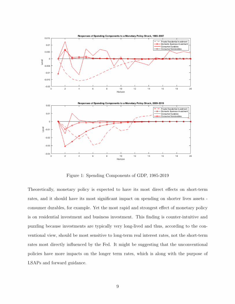
Figure 1: Spending Components of GDP, 1985-2019

Theoretically, monetary policy is expected to have its most direct effects on short-term

rates, and it should have its most significant impact on spending on shorter lives assets -

consumer durables, for example. Yet the most rapid and strongest effect of monetary policy

is on residential investment and business investment. This finding is counter-intuitive and

puzzling because investments are typically very long-lived and thus, according to the con-

ventional view, should be most sensitive to long-term real interest rates, not the short-term

rates most directly influenced by the Fed. It might be suggesting that the unconventional

policies have more impacts on the longer term rates, which is along with the purpose of

LSAPs and forward guidance.

9

2.2 Responses from Banks’ Balance Sheet

In this section I substitute the spending components in the previous VAR system with all

commercial banks’ total deposits, total loans and total security holdings. The data is revealed

by the Federal Reserve every month. The log levels of each of three bank balance-sheet

variables are all deflated by the CPI. I calculated the implied impulse response functions to

a monetary policy shock. In the conventional perspective, banks deposits are expected to

fall following in contraction monetary policy shock, because of the banks’ lending channel

in transmission. The asset components: loans and security holdings, behave differently.

The fall in assets shall mostly concentrated on the decline in security holdings, and total

loans hardly move because loans are quasi-contractual commitments whose stock is difficult

to change immediately. When facing an unanticipated increase in the policy rate, and fall

deposits, banks react to the shock by selling securities quickly. However, security holdings

begin gradually to be rebuilt, as banks re-balance their portfolios, and this is the time when

loans start to fall significantly.

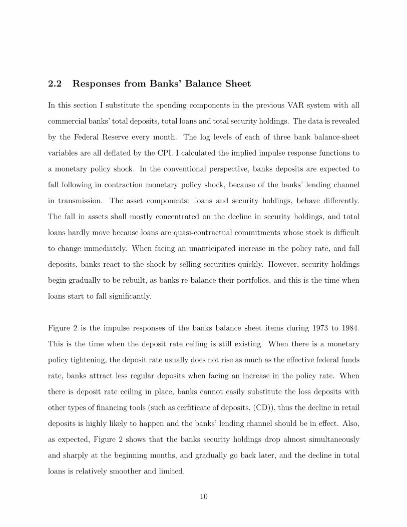
Figure 2 is the impulse responses of the banks balance sheet items during 1973 to 1984.

This is the time when the deposit rate ceiling is still existing. When there is a monetary

policy tightening, the deposit rate usually does not rise as much as the effective federal funds

rate, banks attract less regular deposits when facing an increase in the policy rate. When

there is deposit rate ceiling in place, banks cannot easily substitute the loss deposits with

other types of financing tools (such as cerfiticate of deposits, (CD)), thus the decline in retail

deposits is highly likely to happen and the banks’ lending channel should be in effect. Also,

as expected, Figure 2 shows that the banks security holdings drop almost simultaneously

and sharply at the beginning months, and gradually go back later, and the decline in total

loans is relatively smoother and limited.

10

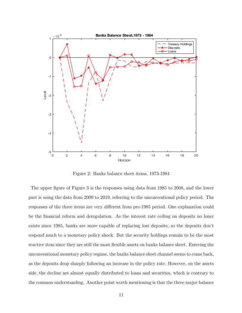
Figure 2: Banks balance sheet items, 1973-1984

The upper figure of Figure 3 is the responses using data from 1985 to 2008, and the lower

part is using the data from 2009 to 2019, referring to the unconventional policy period. The

responses of the three items are very different from pre-1985 period. One explanation could

be the financial reform and deregulation. As the interest rate ceiling on deposits no loner

exists since 1985, banks are more capable of replacing lost deposits, so the deposits don’t

respond much to a monetary policy shock. But the security holdings remain to be the most

reactive item since they are still the most flexible assets on banks balance sheet. Entering the

unconventional monetary policy regime, the banks balance sheet channel seems to come back,

as the deposits drop sharply following an increase in the policy rate. However, on the assets

side, the decline are almost equally distributed to loans and securities, which is contrary to

the common understanding. Another point worth mentioning is that the three major balance

11

Figure 3: Banks balance sheet items, 1985 - 2019

sheet items all respond very limited to a monetary policy shock, which may indicate that the

unconventional policies do not work through the traditional bank transmission mechanism

that much as before.

Figure 5 shows the responses from some deposit items: time deposit and brokered deposit

on commercial banks’ balance sheet. A time deposit is interest bearing and has a pre-set

date of maturity. A certificate of deposit (CD) is one of the typical examples. Time deposits

usually pay higher interest rate than a regular savings account, and longer the maturity is,

higher the interest rate would be. A brokered deposit is a type of deposit made to a bank

with the assistance of a third-party broker. Deposit brokers facilitate the placement of other

people’s deposits with banks and banks sell large denomination deposits to deposit brokers,

who divide these large deposits into smaller investments sold to individual investors. Individ-

12

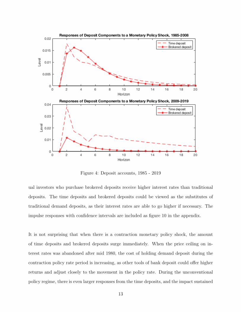
Figure 4: Deposit accounts, 1985 - 2019

ual investors who purchase brokered deposits receive higher interest rates than traditional

deposits. The time deposits and brokered deposits could be viewed as the substitutes of

traditional demand deposits, as their interest rates are able to go higher if necessary. The

impulse responses with confidence intervals are included as figure 10 in the appendix.

It is not surprising that when there is a contraction monetary policy shock, the amount

of time deposits and brokered deposits surge immediately. When the price ceiling on in-

terest rates was abandoned after mid 1980, the cost of holding demand deposit during the

contraction policy rate period is increasing, as other tools of bank deposit could offer higher

returns and adjust closely to the movement in the policy rate. During the unconventional

policy regime, there is even larger responses from the time deposits, and the impact sustained

13

for a very long period. This might be an indication that people believe that the unconven-

tional policies also influence the longer term rates substantially and are will to invest in fixed

return investment pays higher than traditional deposits.

2.3 Responses from Banks’ Loans

In this section I run a detailed investigation into the commercial banks’ major loan portfolios.

Figure 5 is an overview of the major loans in all commercial banks in the United States.

The loans backed up by real properties are the major type of loans, and shows the fastest

growth among all loan categories. Commercial and industrial loans are the second largest

by volume, and presents close connection with the business cycle. Consumer and personal

loans are the most stable category. The sudden jump in the beginning of 2010 was due to an

adjustment in accounting and report regulations, and besides that it shows relatively smooth

growth trend.

I substitute the banks’ balance sheet item in the previous VAR system with these detailed

loan categories and try to capture the responses of these loan items to an unanticipated con-

tractionary monetary policy shock. Also, the full sample expands from 1985 to 2019, and I

separate it into great moderation period and unconventional policy period, to see whether the

unconventional policies make difference on the responses of loans to contractionary shocks.

Figure 5 reports the impulse responses.

Some micro level evidence are provided on how the macro economy and commercial banks

react to monetary policy rate shocks during great moderation and great recession, where

there is no deposit interest rate ceiling and unconventional policies are introduced. The

first thing worth discussing is that the responses to unconventional policies are very mini-

14

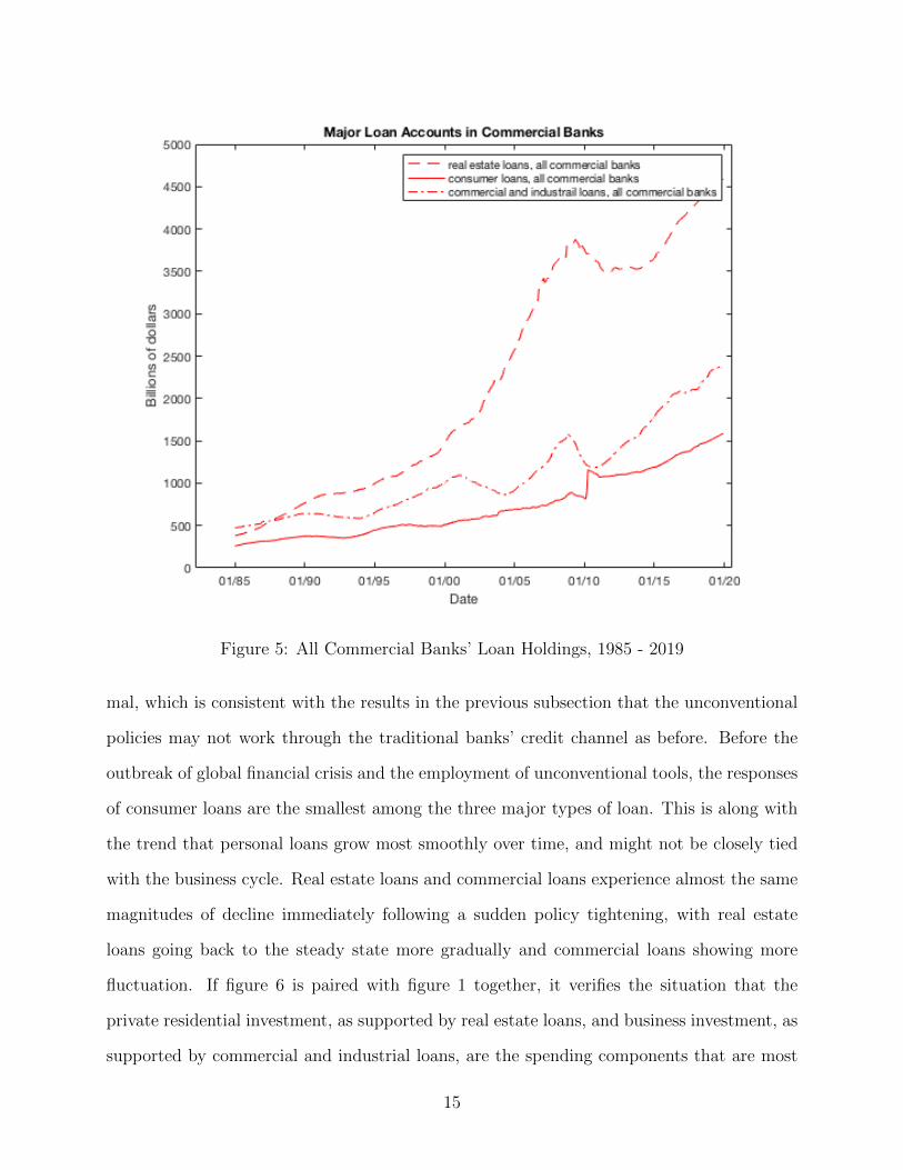
Figure 5: All Commercial Banks’ Loan Holdings, 1985 - 2019

mal, which is consistent with the results in the previous subsection that the unconventional

policies may not work through the traditional banks’ credit channel as before. Before the

outbreak of global financial crisis and the employment of unconventional tools, the responses

of consumer loans are the smallest among the three major types of loan. This is along with

the trend that personal loans grow most smoothly over time, and might not be closely tied

with the business cycle. Real estate loans and commercial loans experience almost the same

magnitudes of decline immediately following a sudden policy tightening, with real estate

loans going back to the steady state more gradually and commercial loans showing more

fluctuation. If figure 6 is paired with figure 1 together, it verifies the situation that the

private residential investment, as supported by real estate loans, and business investment, as

supported by commercial and industrial loans, are the spending components that are most

15

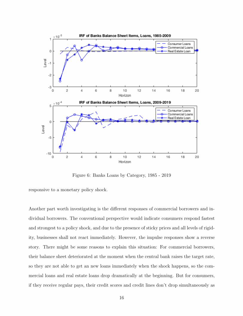
Figure 6: Banks Loans by Category, 1985 - 2019

responsive to a monetary policy shock.

Another part worth investigating is the different responses of commercial borrowers and in-

dividual borrowers. The conventional perspective would indicate consumers respond fastest

and strongest to a policy shock, and due to the presence of sticky prices and all levels of rigid-

ity, businesses shall not react immediately. However, the impulse responses show a reverse

story. There might be some reasons to explain this situation: For commercial borrowers,

their balance sheet deteriorated at the moment when the central bank raises the target rate,

so they are not able to get an new loans immediately when the shock happens, so the com-

mercial loans and real estate loans drop dramatically at the beginning. But for consumers,

if they receive regular pays, their credit scores and credit lines don’t drop simultaneously as

16

the policy rate goes up. There would be using more credits and paying back debts slower.

So the responses of consumer loans are relatively moderate.

3 Empirical Methods using Bank Level Data

3.1 Data Description

In this section, I employ the data collected in Reports of Condition and Income (Call Re-

ports). The CALL report provides very sophisticated individual bank level sources for de-

tailed interest expenses and loan amounts for all insured commercial banks operating in the

United States. I use the data on banks balance sheet and income statement spanning from

the first quarter of 1985 till the last quarter of 2018. The time frame covers both great

moderation and great recession. The total number of bank-quarter observations is 217613.

All implausible negative and zero entries have been removed to ensure the data consistency.

Also, to correct the survival bias, I include only banks that have operation history of five

years or longer. The major item under consideration as the bank level year to year growth of

loans, which is also the main dependent variable. Other variables include the bank specific

data: bank size as measured by total assets, capitalization as measured by capital to asset

ratio, and securitization as measured by security holdings to asset ratio.

Some macroeconomics data are also added into the empirical methodology. The most im-

portant macroeconomic control is the monetary policy, and in the main regression, it is

represented by change in the previous quarter’s federal funds rate. As illustrated in the

previous sections, the federal funds rate is substituted with the shadow rate in order to cap-

ture the negative real rate during the great recession. Another macroeconomic control is the

real gross domestic product growth. So in line with the literature, I add log real industrial

17

production index into this regression. I also consider the effect of the financial crisis and I

am interested in testing whether the its occurrence has reshaped the banks transmission of

monetary policy. So I add a dummy variable which takes the value one if the observation

date is after the third quarter of 2008, and takes the zero if the observation is before crisis.

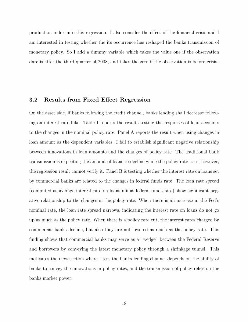
3.2 Results from Fixed Effect Regression

On the asset side, if banks following the credit channel, banks lending shall decrease follow-

ing an interest rate hike. Table 1 reports the results testing the responses of loan accounts

to the changes in the nominal policy rate. Panel A reports the result when using changes in

loan amount as the dependent variables. I fail to establish significant negative relationship

between innovations in loan amounts and the changes of policy rate. The traditional bank

transmission is expecting the amount of loans to decline while the policy rate rises, however,

the regression result cannot verify it. Panel B is testing whether the interest rate on loans set

by commercial banks are related to the changes in federal funds rate. The loan rate spread

(computed as average interest rate on loans minus federal funds rate) show significant neg-

ative relationship to the changes in the policy rate. When there is an increase in the Fed’s

nominal rate, the loan rate spread narrows, indicating the interest rate on loans do not go

up as much as the policy rate. When there is a policy rate cut, the interest rates charged by

commercial banks decline, but also they are not lowered as much as the policy rate. This

finding shows that commercial banks may serve as a ”wedge” between the Federal Reserve

and borrowers by conveying the latest monetary policy through a shrinkage tunnel. This

motivates the next section where I test the banks lending channel depends on the ability of

banks to convey the innovations in policy rates, and the transmission of policy relies on the

banks market power.

18

Table 1: Responses of Loan Amounts and Loan Rate Spread on Policy Rate Change

log(loan)t,i

log(loan)t−1,i 0.953ˆ***(0.004)

∆FFRt−1 0.180ˆ***(0.029)

(a) Panel A

LoanSpreadt,i

LoanSpreadt−1,i 0.880ˆ***(0.008)

∆FFRt−1 -0.587ˆ***(0.030)

(b) Panel A

The table reports the regression results on the equation: yi,t = αi + β1yi,t−1β2∆FFt−i + εit. In panel A,

the dependent variable is the log level of total amount in each commercial bank. In panel B, the dependent

variable is the loan spread, computed as the average interest rate charge on loans minus the target rate. All

coefficients are reported with their standard deviations in parenthesis and significance level.

As inspired by Drechsler, Savov and Schnabl(2017)[12], I define a bank’s Spread Beta

(βSpread) by running Equation (1) for each bank in my defined data set.

∆yit = αi +4∑

τ=0

βτi ∆FFt−τ + εit (1)

∆FFt is the change in the Fed Funds rate from date date t to t + 1. Four periods of lags

is allowed because it takes time for banks to reset non-zero maturity deposit (loan) rates.1

βSpreadi =∑4

τ=0 βτi . The dependent variable ∆yit is the loan spread (computed as average

interest rate on loans minus federal funds rate) of each bank at time t. The Spread Beta

can be interpreted as a measurement of banks responsiveness to the change in policy rate.

Larger Spread Beta indicated more active response to policy innovation. Next I compute

each bank’s Flow Beta by rerunning the same regression but substitute the changes spread

with the changes in loan amounts as the dependent variable. So the Flow Beta can be

viewed as the change in the amount of loans when there is a change in the policy rate. In

the third step, I cluster all commercial banks into at most 100 bins by their Spread Beta.

The highest Spread Beta indicates the bank is very responsive to the policy rate: it actively

raise or cut the interest rate on loans in response to the fluctuations of monetary policies. I

1The lag order follows the setting in Drechsler, Savoy and Schnabl (2017)

19

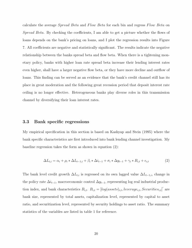
calculate the average Spread Beta and Flow Beta for each bin and regress Flow Beta on

Spread Beta. By checking the coefficients, I am able to get a picture whether the flows of

loans depends on the bank’s pricing on loans, and I plot the regression results into Figure

7. All coefficients are negative and statistically significant. The results indicate the negative

relationship between the banks spread beta and flow beta. When there is a tightening mon-

etary policy, banks with higher loan rate spread beta increase their lending interest rates

even higher, shall have a larger negative flow beta, or they have more decline and outflow of

loans. This finding can be served as an evidence that the bank’s credit channel still has its

place in great moderation and the following great recession period that deposit interest rate

ceiling is no longer effective. Heterogeneous banks play diverse roles in this transmission

channel by diversifying their loan interest rates.

3.3 Bank specific regressions

My empirical specification in this section is based on Kashyap and Stein (1995) where the

bank specific characteristics are first introduced into bank lending channel investigation. My

baseline regression takes the form as shown in equation (2):

∆Lt,i = αi + ρi ∗ ∆Lt−1,i + βi ∗ ∆it−1 + σi ∗ ∆yt−1 + γi ∗Bi,t + εi,t (2)

The bank level credit growth ∆Lt,i is regressed on its own lagged value ∆Lt−1,i, change in

the policy rate ∆it−1, macroeconomic control ∆yt−1, representing log real industrial produc-

tion index, and bank characteristics Bi,t. Bi,t = [log(assets)i,t, leveragei,t, Securitiesi,t]′

are

bank size, represented by total assets, capitalization level, represented by capital to asset

ratio, and securitization level, represented by security holdings to asset ratio. The summary

statistics of the variables are listed in table 1 for reference.

20

Figure 7: Bank loan rate spread and bank level outcome

I estimate the Total Loan Spread Beta for each bank in the sample. The Spread Beta on the vertical axis is estimatedusing the equation: ∆yit = αi +

∑4τ=0 β

τi ∆FFt−τ + εit, where δyit is the change in the loan spread (calculated as

the average interest rate on loans minus federal funds rate) of bank i from date t to t + 1 and ∆FFt is the change in

the Fed Funds rate from date date t to t + 1. The Spread Beta of bank i equals∑4τ=0 β

τi . The Flow Beta of each

major loan product (commercial and industrial loan, real estate loan, personal loan) is estimated using the samemethodology as Spread Beta, but rerunning the same regression with the log growth of C& I loans, loans supportedby real properties, and personal loans, and I refer the sensitivities of these flows to the change in federal funds rate asFlow Beta. The third step is estimating the relationship between Loan Spread Beta and its corresponding Flow Beta.I sort banks into at most a hundred bins by their total loan spread betas. A higher spread beta indicates that banksare more responsive to a change in the monetary policy. I compute the average spread beta and flow beta in each binand regress average flow beta on average spread beta.

21

Notations of variables are interpreted as followed: αi is the bank fixed effect. Bi stands for a

vector of each bank’s specific controls, including Dep: Deposit Ratio; ln(Assets): log(total

asset); Lev: Leverage Ratio; Sec: Securitization Ratio. There are a few reasons to support

my choice of bank specific variables. Dep, deposit ratio, is calculates as bank’s total deposit

divided by its total liability. This is a common variable to measure a bank’s funding reli-

ability on deposits. Total asset is included to evaluate the size of the bank. Lev, leverage

ratio, computed as bank’s total capital divided by its total asset, as the standard Tier I ratio

that has been adopted as part of the Basel III Accord on bank regulation. It’s included to

measure a bank’s financial strength. The inclusion of securitization ratio is to align with the

new business model of banks: from ”originate and hold” to ”originate, repack and sell”. The

variable ∆it−1 is the indicator of monetary policy innovation, and takes the Federal funds

rate in the previous quarter. I use shadow rate instead of FFR after 2008 Q4. C is a dummy

variable from my construction referring to the time period of financial crisis or not. C equals

0 before fourth quarter of 2008 and 1 for the rest of the times.

In the following section, to learn better about the interaction relations of the monetary

policies and bank characteristics, I modify the baseline regression in equation 2 by adding

some dummy variables and interactive variables. I separate the time horizon into before and

after the great recession by including a time dummy. I include some interactive variables to

verify whether some bank specific features could help amplify the bank’s lending channel.

22

∆Lt,i = αi + ρi ∗ ∆Lt−1,i + βi ∗ ∆it−1 + σi ∗ ∆yt−1 + γi ∗Bi,t

+ ψi ∗ ∆it−1 ∗ Ci,t

+ φi ∗ ∆it−1 ∗Bi,t

+ κ ∗ ∆it−1 ∗Bi,t ∗ Ci,t + εi,t

(3)

Before running the regression, I listed some of the key hypothesis that I target to test and

verify. (1)The impact of the change in the target rate on the banks lending behaviors, which

is the coefficient (βi) being estimated in front of the ∆it−1 in equation (3). It is believed

to be significantly negatively if the decrease in the federal funds rate helps to increase the

amount of loans that commercial banks make, and could be viewed as a verification towards

the existence of the bank lending channel. (2) How bank specific features can impact the

transmission of monetary policies. For bank specific controls, I have leverage ratio, securiti-

zation ratio and deposit ratio in the regression. Leverage ratio is proposed to have positive

impact on the growth of loans as well capitalized banks should be more likely to expand

supply of loans. γi,Lev should be positive. Deposit ratio is working in a similar way that

banks with more deposits as funding shall have more supply of funds as loans. γi,Dep should

also show positive sign. Also, for banks with higher holdings of securities, securitization

should be able to work as a source of capital relief, so it is supposed to be also positively

linked with the amount of loans. γi,Sec is regarded as positive.

Some interaction terms are harder to predict in an economic manner. The sign in front

of ∆it−1 ∗Ci,t, (ψi) is ambiguous as the financial crisis and unconventional monetary policies

can either amplify or dampen the traditional bank lending channel. Higher level of securi-

tization is another trend in modern banks balance sheet as banks have accumulated more

treasury holdings and mortgage backed securities, however, the interaction between security

holdings and great recession is also open to debate as higher securitization level may make

23

banks balance sheet more vulnerable facing the financial crisis. Table 4 in the appendix is a

list of all regressors in the equation, with their variable description, expected sign, and my

arguments to explain the expectations.

3.4 Empirical Results

Table 2 summarizes the regression results on equation (3). The growth in the total loans is

the dependent variable and the first column lists the regressors. The second column records

the estimated coefficients for the independent variables. I also switch the dependent vari-

ables with major loan categories, respectively commercial and industrial loans, loans backed

up by real properties, and personal loans, and column 4,5, and 6 report their estimated

coefficients correspondingly. The standard errors are all recorded in the parenthesis below

the coefficient, and significant level is marked by asterisks.

The negative coefficient attached to the policy rate suggests that a tightening monetary

policy leads to the decline in the loan amounts, which could be served as an evidence for the

bank lending channel. This effect is amplified by the great recession. In normal times, a one

percent hike in the policy rate would generate 0.4% drop in the total loan amount. During

the financial crisis, this effect is enlarged by 0.072%, but the difference in total loan amount

is not statistically significant. Among the three major loan categories, personal loans is the

only type of loans that shows this amplified effect at significant level. Personal loans have

a negative relation with the policy rate, and this relation is enlarged after 2008. This could

be interpreted that the drop in the policy rate helps to boost the banks lending during the

financial crisis, and the personal loans surge the most during this period. Contrarily, the

other two categories, commercial loans and real estate loans, both show negative and signifi-

cant relations with the policy rate, but the relations are countered during the great recession.

24

Banks’ heterogeneity in capital ratio and liquidity level account for a vital part in their

transmission of monetary policies. The liquidity ratio is supposed to be positively related

to the amount of loan outstanding. Banks with more liquid balance sheets shall be able to

keep their original credit portfolios when a sudden rise in policy rate. In other words, higher

liquidity ratio make banks have more buffers towards unanticipated policy shocks. The re-

gression results show significant and positive sign in regard to the liquidity level (calculated as

capital to asset ratio), which matches my expectation and is consistent with major thoughts

in the literature. The interaction between liquidity level and monetary policy is also positive

and statistically significant. This result indicates that lending in banks with higher liquidity

show less responses to unanticipated policy rate shocks. However, this pattern is reversed

after the adoption of unconventional policies during the great recession. After 2008, lending

from more liquid banks react more towards monetary policy innovations. Another result

worth future exploring is the bank size. I obtain significant negative coefficients attached

with log total assets. The size of bank, if measured by its total assets, does not help to

explain the decline in banks’ loan during a tightening monetary policy. Compared to smaller

banks, large banks do not necessarily outperform small banks in keeping less lost in loans

portfolios during the adverse monetary policy shocks.

The effect of securitization level is also interesting. Referring to the interaction of policy

rate and securitization level, it is suggested that securitization is positively correlated with

the bank lending channel, but there does not show any significant in the coefficients. If all

other variables are kept constant, banks that have more of their assets securitized should

experience higher growth in lending and loans. These findings are contrary to the tradi-

tional viewpoints. My result shows that banks with better access to the security market

are not necessarily more capable to buffer their lending performance against contractionary

policy shocks. However, securitization plays a more crucial role during the financial crisis

25

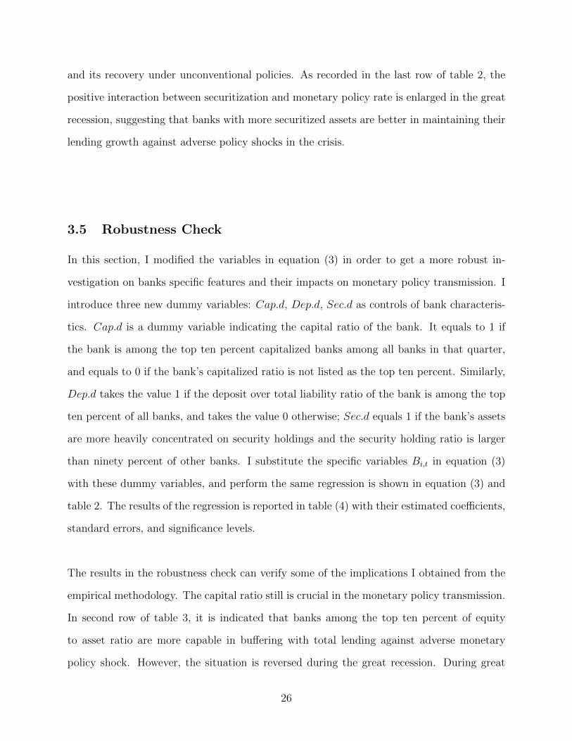
and its recovery under unconventional policies. As recorded in the last row of table 2, the

positive interaction between securitization and monetary policy rate is enlarged in the great

recession, suggesting that banks with more securitized assets are better in maintaining their

lending growth against adverse policy shocks in the crisis.

3.5 Robustness Check

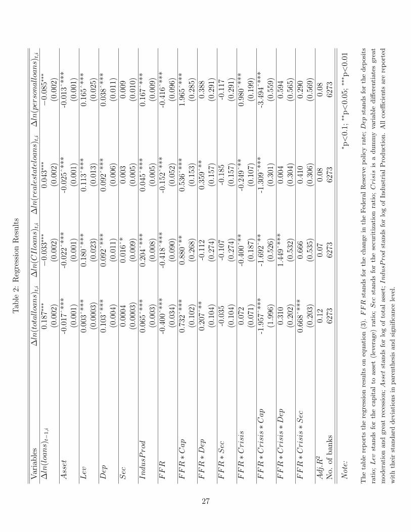
In this section, I modified the variables in equation (3) in order to get a more robust in-

vestigation on banks specific features and their impacts on monetary policy transmission. I

introduce three new dummy variables: Cap.d, Dep.d, Sec.d as controls of bank characteris-

tics. Cap.d is a dummy variable indicating the capital ratio of the bank. It equals to 1 if

the bank is among the top ten percent capitalized banks among all banks in that quarter,

and equals to 0 if the bank’s capitalized ratio is not listed as the top ten percent. Similarly,

Dep.d takes the value 1 if the deposit over total liability ratio of the bank is among the top

ten percent of all banks, and takes the value 0 otherwise; Sec.d equals 1 if the bank’s assets

are more heavily concentrated on security holdings and the security holding ratio is larger

than ninety percent of other banks. I substitute the specific variables Bi,t in equation (3)

with these dummy variables, and perform the same regression is shown in equation (3) and

table 2. The results of the regression is reported in table (4) with their estimated coefficients,

standard errors, and significance levels.

The results in the robustness check can verify some of the implications I obtained from the

empirical methodology. The capital ratio still is crucial in the monetary policy transmission.

In second row of table 3, it is indicated that banks among the top ten percent of equity

to asset ratio are more capable in buffering with total lending against adverse monetary

policy shock. However, the situation is reversed during the great recession. During great

26

Tab

le2:

Reg

ress

ion

Res

ult

s

Var

iable

s∆ln

(totalloans)t,i

∆ln

(CIloans)t,i

∆ln

(realestateloans)t,i

∆ln

(personalloans)t,i

∆ln

(loans)t−

1,i

0.18

7∗∗∗

−0.

033∗

∗∗0.

043∗

∗∗−

0.08

5∗∗∗

(0.0

02)

(0.0

02)

(0.0

02)

(0.0

02)

Asset

-0.0

17ˆ*

**-0

.022

ˆ***

-0.0

25ˆ*

**-0

.013

ˆ***

(0.0

01)

(0.0

01)

(0.0

01)

(0.0

01)

Lev

0.00

3ˆ**

*0.

180ˆ

***

0.11

3ˆ**

*0.

165ˆ

***

(0.0

003)

(0.0

23)

(0.0

13)

(0.0

25)

Dep

0.10

3ˆ**

*0.

092ˆ

***

0.09

2ˆ**

*0.

038ˆ

***

(0.0

04)

(0.0

11)

(0.0

06)

(0.0

11)

Sec

0.00

040.

016ˆ

*0.

003

0.00

9(0

.000

3)(0

.009

)(0

.005

)(0

.010

)IndusProd

0.06

5ˆ**

*0.

204ˆ

***

0.04

5ˆ**

*0.

167ˆ

***

(0.0

03)

(0.0

08)

(0.0

05)

(0.0

09)

FFR

-0.4

00ˆ*

**-0

.418

ˆ***

-0.1

52ˆ*

**-0

.416

ˆ***

(0.0

34)

(0.0

90)

(0.0

52)

(0.0

96)

FFR∗Cap

0.73

2ˆ**

*0.

880ˆ

**0.

536ˆ

***

1.96

5ˆ**

*(0

.102

)(0

.268

)(0

.153

)(0

.285

)FFR∗Dep

0.20

7ˆ**

-0.1

120.

359ˆ

**0.

388

(0.1

04)

(0.2

74)

(0.1

57)

(0.2

91)

FFR∗Sec

-0.0

35-0

.107

-0.1

85-0

.117

(0.1

04)

(0.2

74)

(0.1

57)

(0.2

91)

FFR∗Crisis

0.07

2-0

.400

ˆ**

-0.2

49ˆ*

*0.

980ˆ

***

(0.0

71)

(0.1

87)

(0.1

07)

(0.1

99)

FFR∗Crisis∗Cap

-1.9

57ˆ*

**-1

.692

ˆ**

-1.3

09ˆ*

**-3

.494

ˆ***

(1.9

96)

(0.5

26)

(0.3

01)

(0.5

59)

FFR∗Crisis∗Dep

0.31

01.

449ˆ

***

0.00

40.

594

(0.2

02)

(0.5

32)

(0.3

04)

(0.5

65)

FFR∗Crisis∗Sec

0.66

8ˆ**

*0.

666

0.41

00.

290

(0.2

03)

(0.5

35)

(0.3

06)

(0.5

69)

Adj.R

20.

120.

070.

080.

08N

o.of

ban

ks

6273

6273

6273

6273

Not

e:∗ p<

0.1;

∗∗p<

0.05

;∗∗

∗ p<

0.01

Th

eta

ble

rep

orts

the

regr

essi

onre

sult

son

equ

ati

on

(3).FFR

stan

ds

for

the

chan

ge

inth

eF

eder

al

Res

erve

poli

cyra

te;Dep

stan

ds

for

the

dep

osi

ts

rati

o;Lev

stan

ds

for

the

cap

ital

toas

set

(lev

erage)

rati

o;Sec

stan

ds

for

the

secu

riti

zati

on

rati

o;Crisis

isa

dum

my

vari

ab

led

iffer

enti

ate

sgre

at

mod

erat

ion

and

grea

tre

cess

ion

;Asset

stan

ds

for

log

of

tota

lass

et;IndusProd

stan

ds

for

log

of

Ind

ust

rial

Pro

du

ctio

n.

All

coeffi

cien

tsare

rep

ort

ed

wit

hth

eir

stan

dar

dd

evia

tion

sin

par

enth

esis

and

sign

ifica

nce

leve

l.

27

Tab

le3:

Reg

ress

ion

Res

ult

s

Var

iable

s∆ln

(totalloans)t,i

∆ln

(CIloans)t,i

∆ln

(realestateloans)t,i

∆ln

(personalloans)t,i

FFR

-0.3

43ˆ*

**-1

.405

-0.2

54ˆ*

-0.1

12ˆ*

(0.0

36)

(0.9

88)

(0.1

01)

(0.0

55)

FFR∗Cap.d

0.50

9ˆ**

*0.

830ˆ

**0.

360ˆ

**1.

464ˆ

***

(0.1

04)

(0.2

75)

(0.1

58)

(0.2

93)

FFR∗Dep.d

0.14

90.

206

0.31

8ˆ*

0.22

3(0

.105

)(0

.275

)(0

.157

)(0

.293

)FFR∗Sec.d

-0.0

34-0

.106

-0.1

86-0

.118

(0.1

04)

(0.2

74)

(0.1

57)

(0.2

91)

FFR∗Crisis

0.05

8-0

.527

ˆ**

-0.3

49ˆ*

*0.

765ˆ

***

(0.0

75)

(0.1

87)

(0.1

13)

(0.2

09)

FFR∗Crisis∗Cap.d

-1.1

60ˆ*

**-1

.118

ˆ*-0

.892

ˆ**

-1.8

93ˆ*

**(0

.204

)(0

.536

)(0

.307

)(0

.570

)FFR∗Crisis∗Dep.d

0.18

31.

324ˆ

*0.

093

0.38

1(0

.203

)(0

.535

)(0

.306

)(0

.569

)FFR∗Crisis∗Sec.d

0.66

0ˆ**

0.66

20.

404

0.28

4(0

.203

)(0

.535

)(0

.306

)(0

.569

)Adj.R

20.

130.

080.

080.

08N

o.of

ban

ks

6273

6273

6273

6273

Not

e:∗ p<

0.1;

∗∗p<

0.05

;∗∗

∗ p<

0.01

Th

eta

ble

rep

orts

the

regr

essi

onre

sult

son

equ

atio

n(3

)w

ith

du

mm

yva

riab

les

toin

dic

ate

the

ban

kle

vel

spec

ific

chara

cter

isti

cs.FFR

stan

ds

for

the

chan

gein

the

Fed

eral

Res

erve

poli

cyra

te;Dep.d

stan

ds

for

the

du

mm

yva

riab

leof

dep

osi

tsra

tio

leve

l;Lev.d

stan

ds

for

du

mm

yva

riab

lere

pre

senti

ng

the

cap

ital

toass

etra

tio;Sec.d

stan

ds

for

the

du

mm

yva

riab

lere

pre

senti

ng

the

secu

riti

zati

on

rati

o;

Crisis

isa

du

mm

yva

riab

led

iffer

enti

ates

grea

tm

od

erati

on

an

dgre

at

rece

ssio

n;

See

det

ail

edd

efin

itio

ns

of

vari

ab

les

inth

ete

xt.

All

coeffi

cien

tsar

ere

por

ted

wit

hth

eir

stan

dar

dd

evia

tion

sin

pare

nth

esis

an

dsi

gn

ifica

nce

level

.

28

moderation, a one percent increase in the federal funds rate leads to a drop in total lending

of 0.343% for the average bank, but leads to an increase in total lending of 0.166% for a

bank that is in the last quantile of the distribution of capital ratio. In great recession when

unconventional policies are in place and the shadow rate is used an the indicator of monetary

policy, a 1% drop in the shadow rate generates 0.058% increase in total lending growth for

an average bank (although the coefficient is not statistically significant), and top capitalized

banks’ total lending drop by 1.1%.

Regarding the securitization level, the insignificant coefficient in row 3 of table 3 suggest

that securitization activities do not significantly impact the transmission of monetary poli-

cies during the great moderation. In great recession, 1% increase in the shadow rate lead to

an increase of 0.718% of growth rate in total lendings among the most active banks in the

securitization market. The significant and positive interaction between securitization and

shadow rate during the great recession is in line with the findings in the previous section,

that under unconventional monetary policies, banks with more access and participation in

securitization activities can mitigate the negative effect of adverse policy shocks on their

credit portfolios.

4 Conclusion

This study focuses on the monetary policy transmission through the commercial banks from

mid 1980. The recent decades witness a new era of macro economy: great moderation with

low macroeconomic volatility and great recession with zero nominal policy rate and uncon-

ventional policies. Questions have been raised on whether the monetary policy innovations

under the new environment still share the traditional bank credit channels to impact the

29

economy. I first investigate the responses from the aggregate demand and its more detailed

spending categories. It is surprising that since 1985, monetary policies have more impact on

purchases of longer lived assets instead of short term items, which contradicts the standard

perspective that shocks on short term rates are mostly affecting the purchases of short live

assets.

I then document one key difference by plotting the impulse responses of banks balance

sheet items: deposits, security holdings and loans: from mid 1980s, or starting at great

moderation, the amount of loans does not necessarily decline following a tightening mone-

tary policy. There are two possible explanations towards this situation: one is that since

great moderation, as the deposit rate ceiling being gradually abandoned, commercial banks

are easier to find substitutes of loss deposits. As states in Koch (2015)[17], deposit rate

ceilings embodied in Regulation Q significantly affected bank lending, and the traditional

bank lending channel weakened with deposit rate deregulation since early 1980s. Another

explanation towards my aggregate level finding is that banks build a more security heavy

asset portfolio. In this case, deposits are not the only and most important source of funding

to make loan. Securities become the most reactive item that banks can adjust to encounter

sudden shocks in monetary policies. In this sense, we see securities being the most responsive

balance sheet account that follows very closely to a monetary policy shock.

However, if check the bank level data instead of the aggregate data, I find that the bank

credit channel is present in a more ”broader” format. At the individual bank’s level, the bank

credit channel in monetary policy transmission still exist and hold during great moderation

and great recession, even though the deposit rate ceiling is abandoned and unconventional

policies are in place. I estimate each commercial bank’s loan spread beta (the measurement

of the bank’s responsiveness on loan pricing when facing a policy rate shock) and loan flow

beta (the measurement of the bank’s adjustments on loan amounts when facing a policy rate

30

shock), and I sort banks into at most a hundred bins from the smallest loan rate spread

beta to the highest spread beta. By regressing the loan flow beta on loan spread beta, the

significant negative coefficient indicated that at individual bank level, when there is a con-

tractionary monetary policy, banks with higher loan rate spread (banks that charge higher

interest rates on loans) lose more loans, compared to banks with lower loan spread beta. In

other words, when there is a hike in the policy rate and all banks would raise the interest

rates they charge on loans, and the banks who raise their interest rate more, would have

more loss and decline in lending.

Another interesting finding in this paper is that the bank specific features: size, leverage

ratio and deposit ratio, play vital roles in banks lending decision, and shape the bank’s level

credit channel. This is consistent with the findings in the traditional bank lending chan-

nel literature. Well capitalized banks, or banks with higher deposits, are less sensitive to

the change in the federal funds rate. They adjust their loan amounts and credit portfolio

less dramatically when facing monetary policy shocks. What is surprising is that the se-

curitization activity, which becomes the new trend in the recent decade in banks’ balance

sheets, does not serve as an important characteristic when banks choose how many loans

they own. But securitization is important in transmitting the monetary policy during the

great recession when unconventional policies are adopted. It does not show any significance

in its interaction with monetary policy alone, or in other words, in normal times securitiza-

tion does not help to shrink or amplify the bank credit channel. However, securitization is

significant in amplifying the transmission of unconventional monetary policies. A possible

explanation is that the unconventional policies majorly consists of large-scale purchase of

treasuries and securities, which is exactly the type of securities that commercial banks hold.

This might help to convey the monetary shocks in an accelerated way through the operation

of commercial banks, and the mechanism of how security holdings reshape the monetary

policy transmission worth further investigating in my future research.

31

Appendix

Figure 8: Impulse responses of spending components in GDP with confidence intervals, greatmoderation

32

Figure 9: Impulse responses of spending components in GDP with confidence intervals, greatrecession

33

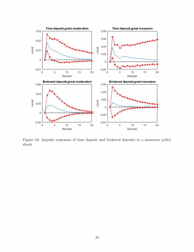
Figure 10: Impulse responses of time deposit and brokered deposits to a monetary policyshock

34

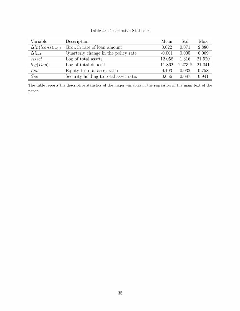
Table 4: Descriptive Statistics

Variable Description Mean Std Max∆ln(loans)t−1,i Growth rate of loan amount 0.022 0.071 2.880∆it−1 Quarterly change in the policy rate -0.001 0.005 0.009Asset Log of total assets 12.058 1.316 21.520log(Dep) Log of total deposit 11.862 1.273 8 21.041Lev Equity to total asset ratio 0.103 0.032 0.758Sec Security holding to total asset ratio 0.066 0.087 0.941

The table reports the descriptive statistics of the major variables in the regression in the main text of the

paper.

35

Tab

le5:

Sum

mar

yof

Reg

ress

ion

Var

iable

s

Dep

ende

nt

vari

able

:∆ln

(loans)t,i

Var

iable

sD

escr

ipti

onE

xp

ecte

dSig

nA

rgum

ent

∆ln

(loans)t−

1,i

Log

oflo

ans

last

quar

ter

∆i t−1

Quar

terl

ych

ange

inth

enom

inal

pol

icy

rate

-T

ighte

nin

gm

onet

ary

pol

icie

sle

adto

de-

clin

ein

lendin

g.Asset

Log

ofto

tal

asse

ts+

/-L

arge

rban

ks

may

bet

ter

isol

ate

adve

rse

shock

s.Lev

Lev

erag

era

tio

+B

anks

wit

hhig

her

leve

rage

rati

ohas

mor

est

able

supply

oflo

ans.

Dep

Dep

osit

rati

o+

Ban

ks

wit

hhig

her

dep

osit

rati

ohas

mor

est

able

supply

oflo

ans.

Sec

Sec

uri

tiza

tion

rati

o,eq

ual

sto

secu

rity

hol

din

gsdiv

ided

by

tota

las

set.

+Sec

uri

tiza

tion

has

som

ere

lief

onfu

ndin

gof

the

ban

k.

Crisis

Cri

sis

dum

my,

equal

sto

0b

efor

e20

08Q

4an

d1

afte

r20

08Q

4∆i t−1∗Crisis

+/-

Inze

ronom

inal

rate

per

iod

the

effec

tof

mon

etar

up

olic

yis

amplified

(-)

orim

-pai

red

(+)

∆i t−1∗Dep

+B

anks

wit

hfe

wer

dep

osit

fundin

gam

plify

mon

etar

yp

olic

ysh

ock

s.∆i t−1∗Sec

+/-

Sec

uri

tiza

tion

amplifies

(+)

orim

pai

rs(-

)m

onet

ary

pol

icy

shock

s.∆i t−1∗Dep

∗Crisis

+B

anks

wit

hfe

wer

dep

osit

fundin

gam

plify

mon

etar

yp

olic

ysh

ock

spar

ticu

larl

ydur-

ing

the

finan

cial

cris

is.

∆i t−1∗Crisis∗Sec

+/-

Sec

uri

tiza

tion

amplifies

(+)

orim

pai

rs(-

)m

onet

ary

pol

icy

shock

sduri

ng

the

finan

-ci

alcr

isis

.T

he

tab

leth

em

ain

vari

able

s,th

eir

not

atio

ns

an

dec

on

om

icw

ise

des

crip

tion

su

sed

inre

gre

ssio

nof

equ

ati

on

2.

Th

eta

ble

als

osu

mm

ari

zes

main

hyp

oth

esis

onth

esi

gns

ofth

ere

gres

sion

coeffi

cien

tsof

thes

eva

riab

les,

an

dec

on

om

icm

ean

ing

an

dex

pla

nati

ons

of

thes

ehyp

oth

esis

.

36

References

[1] A. B. Ashcraft. New evidence on the lending channel. Journal of Money, Credit and

Banking, pages 751–775, 2006.

[2] B. S. Bernanke. Monetary policy since the onset of the crisis. In Federal Reserve Bank

of Kansas City Economic Symposium, Jackson Hole, Wyoming, volume 31, pages 0–24,

2012.

[3] B. S. Bernanke and M. Gertler. Inside the black box: the credit channel of monetary

policy transmission. Journal of Economic perspectives, 9(4):27–48, 1995.

[4] F. Bianchi and L. Melosi. Escaping the great recession. American Economic Review,

107(4):1030–58, 2017.

[5] F. Black. Interest rates as options. the Journal of Finance, 50(5):1371–1376, 1995.

[6] M. K. Brunnermeier and Y. Sannikov. International credit flows and pecuniary exter-

nalities. American Economic Journal: Macroeconomics, 7(1):297–338, 2015.

[7] L. J. Christiano and M. Eichenbaum. Liquidity effects and the monetary transmission

mechanism. Technical report, National Bureau of Economic Research, 1992.

[8] L. J. Christiano, M. S. Eichenbaum, and M. Trabandt. Understanding the great reces-

sion. American Economic Journal: Macroeconomics, 7(1):110–67, 2015.

[9] M. Di Maggio and M. Kacperczyk. The unintended consequences of the zero lower

bound policy. Journal of Financial Economics, 123(1):59–80, 2017.

[10] P. Disyatat. The bank lending channel revisited. Journal of money, Credit and Banking,

43(4):711–734, 2011.

[11] L. Drager and G. Nghiem. Are consumers’ spending decisions in line with an euler

equation? Review of Economics and Statistics, pages 1–45, 2018.

37

[12] I. Drechsler, A. Savov, and P. Schnabl. The deposits channel of monetary policy. The

Quarterly Journal of Economics, 132(4):1819–1876, 2017.

[13] J. Eisenshmidt and F. Smets. Negative interest rates: Lessons from the euro area. Series

on Central Banking Analysis and Economic Policies no. 26, 2019.

[14] L. Gambacorta and D. Marques-Ibanez. The bank lending channel: lessons from the

crisis. Economic Policy, 26(66):135–182, 2011.

[15] R. S. Gurkaynak, B. Sack, and J. H. Wright. The us treasury yield curve: 1961 to the

present. Journal of monetary Economics, 54(8):2291–2304, 2007.

[16] A. Jobst and H. Lin. Negative interest rate policy (NIRP): implications for monetary

transmission and bank profitability in the euro area. International Monetary Fund, 2016.

[17] C. Koch. Deposit interest rate ceilings as credit supply shifters: Bank level evidence on

the effects of regulation q. Journal of Banking & Finance, 61:316–326, 2015.

[18] A. Krishnamurthy and A. Vissing-Jorgensen. The effects of quantitative easing on

interest rates: channels and implications for policy. Technical report, National Bureau

of Economic Research, 2011.

[19] F. S. Mishkin. The channels of monetary transmission: lessons for monetary policy.

Technical report, National Bureau of Economic Research, 1996.

[20] C. A. Sims and T. Zha. Error bands for impulse responses. Econometrica, 67(5):1113–

1155, 1999.

[21] J. C. Stroebel and J. B. Taylor. Estimated impact of the fed’s mortgage-backed securities

purchase program. Technical report, National Bureau of Economic Research, 2009.

[22] J. C. Wu and F. D. Xia. Measuring the macroeconomic impact of monetary policy at

the zero lower bound. Journal of Money, Credit and Banking, 48(2-3):253–291, 2016.

38

[23] J. L. Yellen. The economic outlook and monetary policy. speech at the

Money Marketeers of New York, New York (April 11), http://www. federalreserve.

gov/newsevents/speech/yellen20120411a. htm-0.2, 2012.

39