the clamped elastic grid, a fourth order equation on …€¦ · the clamped elastic grid, a fourth...
TRANSCRIPT

The clamped elastic grid,a fourth order equationon a domain with corner

The clamped elastic grid,a fourth order equationon a domain with corner
Proefschrift
ter verkrijging van de graad van doctoraan de Technische Universiteit Delft,
op gezag van de Rector Magnificus Prof. dr. ir. J.T. Fokkema,voorzitter van het College voor Promoties,
in het openbaar te verdedigenop dinsdag 29 september 2009 om 10.00 uur
door
Tymofiy GERASIMOV
Master of Science in Applied MathematicsZaporizhzhia Staatsuniversiteit, Oekraıne
geboren te Leninabad, Sovjet Unie
Dit proefschrift is goedgekeurd door de promotor:
Prof. dr. G.H. Sweers
Samenstelling promotiecommissie:
Rector Magnificus, Technische Universiteit Delft, voorzitterProf. dr. G.H. Sweers, Technische Universiteit Delft &
Universitat zu Koln, promotorProf. C. Davini, Universita degli Studi di UdineProf. dr. B. Kawohl, Universitat zu KolnProf. dr. ir. A.W. Heemink, Technische Universiteit DelftProf. dr. J.M.A.M. van Neerven, Technische Universiteit DelftProf. dr. ir. C. Vuik, Technische Universiteit DelftDr. ir. E.H. van Brummelen, Technische Universiteit Delft
Prof. ir. L. van der Sluis, Technische Universiteit Delft, reservelid
ISBN 978-90-9024623-9
Copyright c© 2009 by T. Gerasimov
Printed in the Netherlands by: Wohrmann Print Service
This research was carried out at the Functional Analysis Group, Delft Instituteof Applied Mathematics, Department of Electrical Engineering, Mathematicsand Computer Science, Delft University of Technology, the Netherlands

To Anna and Liza,
who give me the strengthin all my accomplishments

Contents
1 Introduction 11.1 The model . . . . . . . . . . . . . . . . . . . . . . . . . . . . . . 11.2 The setting . . . . . . . . . . . . . . . . . . . . . . . . . . . . . 3
1.2.1 Why grid model? Mathematical motivation . . . . . . . 41.2.2 Why corner? Mechanical motivation . . . . . . . . . . . 5
1.3 The target . . . . . . . . . . . . . . . . . . . . . . . . . . . . . . 71.4 Content of the thesis . . . . . . . . . . . . . . . . . . . . . . . . 10
2 Existence and uniqueness 132.1 Approach outline . . . . . . . . . . . . . . . . . . . . . . . . . . 132.2 Properties of the energy functional . . . . . . . . . . . . . . . . 142.3 Weak solution, existence and uniqueness result . . . . . . . . . 18
3 Homogeneous problem in an infinite cone 193.1 Reduced problem . . . . . . . . . . . . . . . . . . . . . . . . . . 193.2 General statements for the eigenvalues λ . . . . . . . . . . . . . 243.3 Analysis of the eigenvalues λ when α = 0 . . . . . . . . . . . . 27
3.3.1 Intermezzo: a comparison with ∆2 . . . . . . . . . . . . 283.4 Analysis of the eigenvalues λ when α = 0 (continued) . . . . . . 30
3.4.1 Behavior of λ in V . . . . . . . . . . . . . . . . . . . . . 323.4.2 Eigenvalue λ1 as the bottom part of Γ . . . . . . . . . . 37
3.5 On the behaviour of ω 7→ λ1(ω), ω ∈ (0, 2π] when α ∈(0, 1
2π)
. 413.6 Structure of solutions to (3.1) in the cone K(α,ω) . . . . . . . . 42
4 Kondratiev’s weighted Sobolev spaces 474.1 Comparing (weighted) Sobolev spaces: imbeddings . . . . . . . 48
vii
viii CONTENTS
5 Regularity results 535.1 General regularity statement . . . . . . . . . . . . . . . . . . . 535.2 Regularity for the singular part of u . . . . . . . . . . . . . . . 575.3 Corollary . . . . . . . . . . . . . . . . . . . . . . . . . . . . . . 605.4 Comparison with the bilaplacian case . . . . . . . . . . . . . . . 61
6 System approach to the clamped grid problem 636.1 Outline and settings . . . . . . . . . . . . . . . . . . . . . . . . 636.2 System approach . . . . . . . . . . . . . . . . . . . . . . . . . . 666.3 Comparing minimizing and system approach . . . . . . . . . . 69
A Algebraic transformation 73A.1 Ellipticity of operator La . . . . . . . . . . . . . . . . . . . . . 73A.2 Transforming the roots . . . . . . . . . . . . . . . . . . . . . . . 75A.3 Duality . . . . . . . . . . . . . . . . . . . . . . . . . . . . . . . 81
B A fundamental system of solutions 83B.1 Derivation of system Sλ . . . . . . . . . . . . . . . . . . . . . . 83B.2 Derivation of systems S−1, S0, S1 . . . . . . . . . . . . . . . . . 84
B.2.1 Case λ = −1 . . . . . . . . . . . . . . . . . . . . . . . . 85B.2.2 Case λ = 0 . . . . . . . . . . . . . . . . . . . . . . . . . 86B.2.3 Case λ = 1 . . . . . . . . . . . . . . . . . . . . . . . . . 87
B.3 The explicit formulas for P−1,P0,P1 . . . . . . . . . . . . . . . 88B.3.1 Case λ = −1 . . . . . . . . . . . . . . . . . . . . . . . . 89B.3.2 Case λ = 0 . . . . . . . . . . . . . . . . . . . . . . . . . 89B.3.3 Case λ = 1 . . . . . . . . . . . . . . . . . . . . . . . . . 91
C Analytical tools for the numerical computations 93C.1 Implicit function and discretization . . . . . . . . . . . . . . . . 93C.2 A version of the Morse theorem . . . . . . . . . . . . . . . . . . 94C.3 The Morse Theorem applied . . . . . . . . . . . . . . . . . . . . 98
C.3.1 Computational results I . . . . . . . . . . . . . . . . . . 99C.3.2 Checking the range for Morse . . . . . . . . . . . . . . . 102
C.4 On the insecting curves from Morse . . . . . . . . . . . . . . . . 104C.4.1 Computational results II . . . . . . . . . . . . . . . . . . 104C.4.2 Strict positivity of the functions ∂h2
∂λ (ω, λ) and16√
2∂h1∂λ (ω, λ) + π ∂h2
∂λ (ω, λ) on U . . . . . . . . . . . . 111C.5 On P (ω, λ) = 0 in V away from a =
(12π, 4
). . . . . . . . . . . 113

CONTENTS ix
C.5.1 Set of Claims I . . . . . . . . . . . . . . . . . . . . . . . 113C.5.2 Set of Claims II . . . . . . . . . . . . . . . . . . . . . . . 122
D Explicit eigenvalues and eigenfunctions 125D.1 Computations for λj∞j=1 . . . . . . . . . . . . . . . . . . . . . 126
D.1.1 Case α = 0, ω = 12π . . . . . . . . . . . . . . . . . . . . 126
D.1.2 Case α ∈[0, 1
2π), ω = π . . . . . . . . . . . . . . . . . . 127
D.1.3 Case α = 0, ω = 32π . . . . . . . . . . . . . . . . . . . . 127
D.1.4 Case α ∈[0, 1
2π), ω = 2π . . . . . . . . . . . . . . . . . 128
D.2 The list of tables for uj,q . . . . . . . . . . . . . . . . . . . . . . 129
E Application of the FreeFem++ package 133E.1 FreeFem++ programming . . . . . . . . . . . . . . . . . . . . . 133
E.1.1 The test problem . . . . . . . . . . . . . . . . . . . . . . 134E.1.2 The code . . . . . . . . . . . . . . . . . . . . . . . . . . 135E.1.3 The results . . . . . . . . . . . . . . . . . . . . . . . . . 136
E.2 Clamped isotropic plate and grid: comparison . . . . . . . . . . 136E.2.1 Ω is a rectangle . . . . . . . . . . . . . . . . . . . . . . . 138E.2.2 Ω is a pentagon . . . . . . . . . . . . . . . . . . . . . . . 140
E.3 Simulations for the DH-106 “Comet” . . . . . . . . . . . . . . . 142
Summary 149
Samenvatting 153
Acknowledgement 157
Curriculum Vitae 159

Chapter 1
Introduction
The operator L = ∂4
∂x4 + ∂4
∂y4can be used as a model for the vertical dis-
placement of a two-dimensional grid that consists of two perpendicular sets ofelastic fibers or rods. We are interested in the behaviour of such a grid that isclamped at the boundary and more specifically near a corner of the domain.Kondratiev supplied the appropriate setting in the sense of Sobolev type spacestailored to find the optimal regularity. Inspired by the Laplacian and the bi-laplacian models one expects, except maybe for some isolated special angles,that the optimal regularity improves when angle decreases. For the homoge-neous Dirichlet problem with this special non-isotropic fourth order operatorL = ∂4
∂x4 + ∂4
∂y4such a result does not hold true. We will prove the existence of
at least one interval(
12π, ω?
), ω?/π ≈ 0.528 (in degrees ω? ≈ 95.1), in which
the optimal regularity improves with increasing opening angle.
1.1 The model
The Kirchhoff model for small deformations of a thin isotropic elastic plate is∆2u = f (see e.g. the seminal paper [17]). Here f is a force density, u is thevertical displacement of a plate and ∆2 = ∂4
∂x4 + 2 ∂4
∂x2∂y2+ ∂4
∂y4is the Bilaplace
operator; the model neglects the influence of horizontal deviations.Non-isotropic elastic plates are still modeled by fourth order differential
equations but the coefficients in front of the derivatives of u may vary. Theinteresting extreme case is the equation
uxxxx + uyyyy = f.
1

2 CHAPTER 1. INTRODUCTION
One may think of the above equation as of the model of an elastic mediumconsisting of two sets of intertwined (not glued) perpendicular fibers runningin Cartesian directions (Figure 1.1). We will call such medium a grid and theoperator L = ∂4
∂x4 + ∂4
∂y4a grid operator.
Figure 1.1: A fragment of an elastic grid.
The main assumption here is that sets of fibers are connected in such away that the vertical positions coincide but there is no connection that forces atorsion in the fibers. Such torsion would occur if the fibers are glued or imbed-ded in a softer medium. For those models see [27]. The appropriate linearizedmodel in that last situation would contain mixed fourth order derivatives.
A first place where operator L = ∂4
∂x4 + ∂4
∂y4appears is J. II. Bernoulli’s
paper [1]. He assumed that it was the appropriate model for an isotropicplate. It was soon dismissed as a model for such a plate, since it failed to haverotational symmetry. Indeed, the rotation of 1
4π transforms ∂4
∂x4 + ∂4
∂y4into
12∂4
∂x4 + 3 ∂4
∂x2∂y2+ 1
2∂4
∂y4.

1.2. THE SETTING 3
1.2 The setting
We will focus on L = ∂4
∂x4 + ∂4
∂y4supplied with homogeneous Dirichlet boundary
conditions. This problem, which we call ‘a clamped grid’, is as follows:uxxxx + uyyyy = f in Ω,
u = ∂∂nu = 0 on ∂Ω.
(1.1)
Here Ω ⊂ R2 is open and bounded, and n is the unit outward normal vectoron ∂Ω. The boundary conditions in (1.1) correspond to the clamped situationmeaning that the vertical position and the angle are fixed to be 0 at theboundary.
One verifies directly that the operator L = ∂4
∂x4 + ∂4
∂y4is elliptic in Ω.
One may also prove, if the normal n is well-defined, that the boundary valueproblem (1.1) is regular elliptic. Indeed, the Dirichlet problem which fixesthe zero and first order derivatives at the boundary, is regular elliptic for anyfourth order uniformly elliptic operator. Hence, under the assumption that Ωis bounded and ∂Ω ∈ C∞ the full classical regularity result (see e.g. [25]) forproblem (1.1) can be used to find for k ≥ 0 and p ∈ (1,∞):
if f ∈W k,p(Ω) then u ∈W k+4,p(Ω). (1.2)
If Ω in (1.1) has a piecewise smooth boundary ∂Ω with, say, one angularpoint, the result (1.2) in general does not apply. Instead, one may use thetheory developed by Kondratiev [18]. This theory provides the appropriatetreatment of problem (1.1) by employing the weighted Sobolev space V k,p
β (Ω)(see Definition 4.1), where k ≥ 0 is the differentiability index and β ∈ Rcharacterizes the powerlike growth of the solution near the angular point ofΩ. Within the framework of the Kondratiev spaces V k,p
β (Ω) the regularityresult “analogous” to (1.2) will then be as follows. There is a countable set offunctions ujj∈N and constants cjj∈N such that for all k ∈ N:
if f ∈ V k,pβ (Ω) then u = w +
J(k,p,β)∑j=1
cjuj with w ∈ V k+4,pβ (Ω).
(1.3)The functions ujj∈N in (1.3) describe the behaviour of the solution u lo-cally in the vicinity of an angular point and are called sometimes the singularsolutions to (1.1). In this thesis, we will restrict our formulations to p = 2.

4 CHAPTER 1. INTRODUCTION
Partial differential equations on domains with corners have obtained a lotof attention both in the mechanical and mathematical literature. For instance,in 1951 Williams in his paper [30] identified possible power singularities fora variety of homogeneous boundary conditions on the plate edges for angularelastic plates in bending treated within classical fourth-order theory. However,one may assume that the advanced qualitative theory on the subject has beendeveloped in the seminal paper by Kondatiev [18]. Since that time manyauthors of which we would like to mention Kozlov, Maz’ya, Rossmann [19, 20],Grisvard [14], Dauge [7], Costabel and Dauge [4], Nazarov and Plamenevsky[26] have contributed. For applications in elasticity theory we refer to Leguillonand Sanchez-Palencia [23], Blum and Rannacher [3]. A recent paper of Kawohland Sweers [21] concerned the positivity question for the operators ∂4
∂x4 +∂4
∂y4and 1
2∂4
∂x4 + 3 ∂4
∂x2∂y2+ 1
2∂4
∂y4in a rectangular domain for hinged boundary
conditions.
1.2.1 Why grid model? Mathematical motivation
We have already mentioned above that the deformation of a thin non-isotropicelastic plate is modeled by the equation (see e.g. [24, p. 281]):
D1uxxxx +D2uxxxy +D3uxxyy +D4uxyyy +D5uyyyy = f,
where Dj , j = 1, ..., 5 are elastic constants of a material a plate made of. Bythe standard rescaling in x and y one may turn the coefficients in front ofuxxxx and uyyyy into 1, so that the abstract mathematical model would be
uxxxx + b1uxxxy + b2uxxyy + b3uxyyy + uyyyy = f,
with bj ∈ R, j = 1, 2, 3. In Appendix A we show that provided the operator∂4
∂x4 + b1∂4
∂x3∂y+ b2
∂4
∂x2∂y2+ b3
∂4
∂x∂y3+ ∂4
∂y4is elliptic, there always exists an
appropriate linear coordinate transformation such that in new coordinates theabove equation will read as
uxxxx + 2auxxyy + uyyyy = f,
with a ∈ [1,+∞). If we set a = 3 in the above equation and rotate thecoordinate system by 1
4π, we will arrive (by further rescaling) at our gridmodel uxxxx + uyyyy = f .

1.2. THE SETTING 5
1.2.2 Why corner? Mechanical motivation
A thin (non-isotropic) elastic plate is the main constructive element of almostevery thin-walled engineering construction ranging from aircrafts, bridges,ships and oil rigs to storage vessels, industrial buildings and warehouses. Aconventional geometry for such a plate is a polygon, that is, a planar domainwith corners (both convex and concave, in general). From an engineeringpractice, it is well known that the presence of corners, namely, the reentrantcorners in a plate may cause a significant reduction or even the loss of itsload-carrying capacity. This happens due to concentration of stresses whichappear near corner points of a plate and which can be extremely high (stresssingularity).
Examples of such a loss are the crashes of De Havilland 106 aircrafts (seeFigure 1.2) in the yearly 1950s. Also known as “The Comet” it was the firstcommercial airliner with jet engines and pressurized fuselage. The designersimplemented cabin’s pressurization in order to provide the passengers with thecomfortable living conditions during the altitude flight. Within the first twoyears after entering service in May 1952, two of the fleet disintegrated whileclimbing to cruise altitude.
Figure 1.2: May 2, 1952. ”The Comet” G-ALYP departures from London’sHeathrow Airport for her first scheduled flight. The picture is taken from [15].
Extensive investigation determined the major constructive weakness of the
6 CHAPTER 1. INTRODUCTION
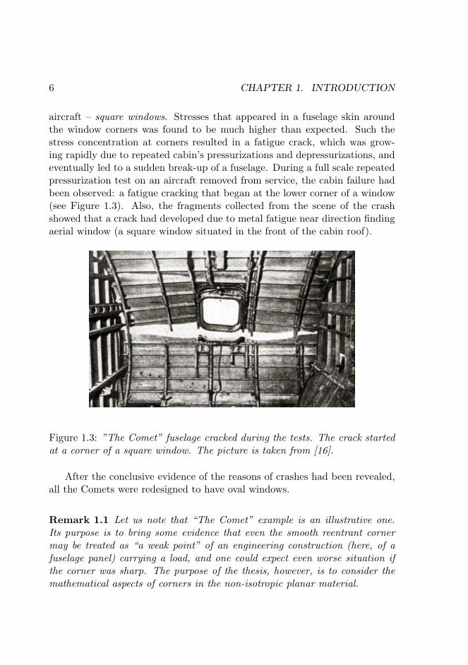
aircraft – square windows. Stresses that appeared in a fuselage skin aroundthe window corners was found to be much higher than expected. Such thestress concentration at corners resulted in a fatigue crack, which was grow-ing rapidly due to repeated cabin’s pressurizations and depressurizations, andeventually led to a sudden break-up of a fuselage. During a full scale repeatedpressurization test on an aircraft removed from service, the cabin failure hadbeen observed: a fatigue cracking that began at the lower corner of a window(see Figure 1.3). Also, the fragments collected from the scene of the crashshowed that a crack had developed due to metal fatigue near direction findingaerial window (a square window situated in the front of the cabin roof).
Figure 1.3: ”The Comet” fuselage cracked during the tests. The crack startedat a corner of a square window. The picture is taken from [16].
After the conclusive evidence of the reasons of crashes had been revealed,all the Comets were redesigned to have oval windows.
Remark 1.1 Let us note that “The Comet” example is an illustrative one.Its purpose is to bring some evidence that even the smooth reentrant cornermay be treated as “a weak point” of an engineering construction (here, of afuselage panel) carrying a load, and one could expect even worse situation ifthe corner was sharp. The purpose of the thesis, however, is to consider themathematical aspects of corners in the non-isotropic planar material.
1.3. THE TARGET 7
1.3 The target
In this thesis, we will focus particularly on the optimal regularity for theclamped grid problem, which depends on the opening angle of the corner. Forthe sake of a simple presentation, we will consider (1.1) in a domain Ω ⊂ R2
which has one corner in 0 ∈ ∂Ω with opening angle ω ∈ (0, 2π]. Due to theKondratiev theory a more appropriate formulation of the problem should readas:
uxxxx + uyyyy = f in Ω,
u = 0 on ∂Ω,∂∂nu = 0 on ∂Ω\0,
(1.4)
“with prescribed growth behaviour near 0”.
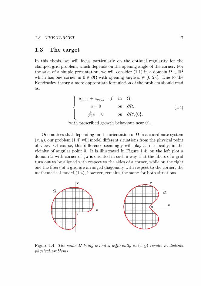
One notices that depending on the orientation of Ω in a coordinate system(x, y), our problem (1.4) will model different situations from the physical pointof view. Of course, this difference seemingly will play a role locally, in thevicinity of angular point 0. It is illustrated in Figure 1.4: on the left plot adomain Ω with corner of 3
2π is oriented in such a way that the fibers of a gridturn out to be aligned with respect to the sides of a corner, while on the rightone the fibers of a grid are arranged diagonally with respect to the corner; themathematical model (1.4), however, remains the same for both situations.
0
y
x
Ω
0
y
x
Ω
Figure 1.4: The same Ω being oriented differently in (x, y) results in distinctphysical problems.

8 CHAPTER 1. INTRODUCTION
Hence, in order to complete the formulation of (1.4), we introduce a para-meter α ∈
[0, 1
2π), which defines orientation of Ω. Obviously, the cases α = 0
and α = 12π yield the identical situation.
The precise description of a domain Ω in problem (1.4) will be then asfollows.
Condition 1.2 The domain Ω has a smooth boundary except at (x, y) = 0,and is such that in the vicinity of 0 it locally coincides with a cone. In otherwords,
1. ∂Ω\0 is C∞,
2. Ω ∩Bε(0) = K(α,ω) ∩Bε(0),
where Bε(0) = (x, y) : |(x, y)| < ε is the open ball of radius ε > 0 centeredat (x, y) = 0 and K(α,ω) an infinite cone with an opening angle ω ∈ (0, 2π] andorientation angle α ∈ [0, 1
2π):
K(α,ω) = (r cos(θ), r sin(θ)) : 0 < r <∞ and α < θ < α+ ω . (1.5)
In Figure 1.5 a domain Ω which satisfies the condition above and corre-sponding cone K(α,ω) are sketched.
0
y
x
Ω
ω α
(α,ω)
0
y
x
Κ
ω α
Figure 1.5: Example for Ω and the corresponding cone K(α,ω).
1.3. THE TARGET 9
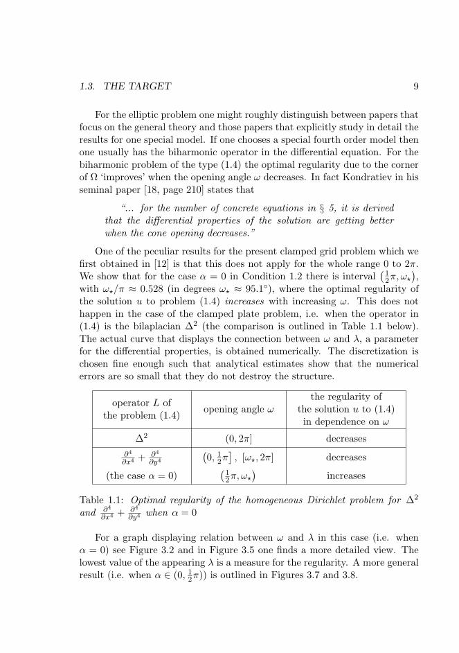
For the elliptic problem one might roughly distinguish between papers thatfocus on the general theory and those papers that explicitly study in detail theresults for one special model. If one chooses a special fourth order model thenone usually has the biharmonic operator in the differential equation. For thebiharmonic problem of the type (1.4) the optimal regularity due to the cornerof Ω ‘improves’ when the opening angle ω decreases. In fact Kondratiev in hisseminal paper [18, page 210] states that
“... for the number of concrete equations in § 5, it is derivedthat the differential properties of the solution are getting betterwhen the cone opening decreases.”
One of the peculiar results for the present clamped grid problem which wefirst obtained in [12] is that this does not apply for the whole range 0 to 2π.We show that for the case α = 0 in Condition 1.2 there is interval
(12π, ω?
),
with ω?/π ≈ 0.528 (in degrees ω? ≈ 95.1), where the optimal regularity ofthe solution u to problem (1.4) increases with increasing ω. This does nothappen in the case of the clamped plate problem, i.e. when the operator in(1.4) is the bilaplacian ∆2 (the comparison is outlined in Table 1.1 below).The actual curve that displays the connection between ω and λ, a parameterfor the differential properties, is obtained numerically. The discretization ischosen fine enough such that analytical estimates show that the numericalerrors are so small that they do not destroy the structure.
operator L ofthe problem (1.4)
opening angle ωthe regularity of
the solution u to (1.4)in dependence on ω
∆2 (0, 2π] decreases∂4
∂x4 + ∂4
∂y4
(the case α = 0)
(0, 1
2π], [ω?, 2π](
12π, ω?
) decreases
increases
Table 1.1: Optimal regularity of the homogeneous Dirichlet problem for ∆2
and ∂4
∂x4 + ∂4
∂y4when α = 0
For a graph displaying relation between ω and λ in this case (i.e. whenα = 0) see Figure 3.2 and in Figure 3.5 one finds a more detailed view. Thelowest value of the appearing λ is a measure for the regularity. A more generalresult (i.e. when α ∈ (0, 1
2π)) is outlined in Figures 3.7 and 3.8.
10 CHAPTER 1. INTRODUCTION
1.4 Content of the thesis
This thesis is divided into six chapters and several appendices.In Chapter 2 we recall the results for existence and uniqueness of a weak
solution u to problem (1.4).Chapter 3 is one of the key parts of this thesis. It studies the homogeneous
problem in the infinite cone K(α,ω),uxxxx + uyyyy = 0 in K(α,ω),
u = 0 on ∂K(α,ω),
∂∂nu = 0 on ∂K(α,ω)\0.
We derive (almost explicitly) a countable set of functions ujj∈N solving thisproblem. These functions describe the behaviour of the weak solution u toproblem (1.4) locally in the vicinity of an angular point 0 of Ω in terms of theangle α and the opening angle ω. They will contribute in Chapter 5 to theregularity statement for u of type (1.3).
In Chapter 4 the weighted Sobolev spaces V l,2β (Ω) are presented and we
recall the imbedding results for W k,2(Ω) and V l,2β (Ω) based on a Hardy in-
equality.Next to this, in Chapter 5 we address the Kondratiev theory and give the
regularity statement for the solution u to our clamped grid problem (1.4) andits asymptotic representation in terms of ujj∈N. We will also compare theresults obtained with those known for the clamped plate problem.
Finally, in Chapter 6 we develop a system approach to our fourth orderproblem (1.4). It is favourized for numerical methods since one may use piece-wise linear C0,1-elements, readily available in standard programming packages.We will show that such a system approach for our clamped grid problem mayfail to produce the correct solution when Ω has a reentrant (concave) corner.
The appendices contain computational and numerical results. Thus, inthe first appendix we prove that every elliptic fourth order operator (which isdefined by three parameters) is, in fact, equivalent to one parametric operator.This result is based on the Mobius transformation. The elaborate third appen-dix confirms that the errors in the numerical computations involved in order toillustrate our analytical results for Chapter 3 are small enough. This appendixalso contains an explicit version of the Morse Theorem, which is necessary foran analytical error bound that confirms the numerical results. In the last ap-

1.4. CONTENT OF THE THESIS 11
pendix, we use the numerical approach developed in Chapter 6 to compare thesolutions to the clamped plate and clamped grid problems when Ω has somespecific geometry. We also simulate the distribution of stresses which appearin “The Comet” fuselage panel with a square and a round window under theuniformly distributed load.

Chapter 2
Existence and uniqueness
For the present so-called clamped boundary conditions existence of an appro-priate weak solution can be obtained in a standard way even when the corneris not convex. We will recall the arguments for the existence of a weak solutionto problem (1.4).
The function space for these weak solutions isW 2,2(Ω) = C∞
c (Ω)‖.‖W2,2(Ω) . (2.1)
where C∞c (Ω) is the space of infinitely smooth functions with compact support
in Ω.
Remark 2.1 For Ω from Condition 1.2, one finds that u ∈W 2,2(Ω) implies
u = 0 on ∂Ω and Du = 0 on ∂Ω\0 in the sense of traces.
Definition 2.2 A function u ∈W 2,2(Ω) is a weak solution of the boundary
value problem (1.4) with f ∈ L2(Ω), if∫Ω
(uxxϕxx + uyyϕyy − fϕ) dxdy = 0 for all ϕ ∈W 2,2(Ω). (2.2)
2.1 Approach outline
We use the direct method in the calculus of variations in order to prove the
existence of a weak solution u ∈W 2,2(Ω) to (1.4) when f ∈ L2(Ω). Let us
outline the method.
13

14 CHAPTER 2. EXISTENCE AND UNIQUENESS
We consider the functional which describes the potential energy stored bythe grid after it has been deformed:
E [u] =∫Ω
(12
(u2xx + u2
yy
)− fu
)dxdy. (2.3)
Due to the type of boundary conditions (the clamped edge), E is defined over
the spaceW 2,2(Ω).
Suppose that there exists a minimizer u ∈W 2,2(Ω) of E. Then the real-
valued function τ(ε) := E [u+ εϕ] has a minimum at ε = 0, meaning thatτ ′(ε)|ε=0 = 0. Hence, for the minimizer u it holds that d
dεE [u+ εϕ]∣∣ε=0
=
0 for all ϕ ∈W 2,2(Ω) and the expansion of the latter condition results in
(2.2). For f ∈ L2(Ω) and provided u satisfying (2.2) is more regular (namely,W 4,2(Ω)), an integration by parts of (2.2) shows that u will fulfill the boundaryvalue problem (1.4) in L2-sense.
Remark 2.3 If Ω in (1.4) is smooth enough, it is straightforward that for
f ∈ L2(Ω) the minimizer u ∈W 2,2(Ω) of (2.3) lies in W 4,2(Ω).
When Ω in (1.4) is as in Condition 1.2 we will see in Chapter 5, Theorem
5.3 that for f ∈ L2(Ω) the minimizer u ∈W 2,2(Ω) has the following represen-
tation u = w+S. Here w lies in W 4,2(Ω) and S is such that Sxxxx+Syyyy = 0in Ω. So, the integration by part in this case also yields that u will fulfill theboundary value problem (1.4) in L2-sense.
In the next Section we study the properties of the functional E in (2.3)
over the spaceW 2,2(Ω) in order to prove that the minimizer of this E exists
and is unique.
2.2 Properties of the energy functional
Due to the form of E it seems to be reasonable (and more appropriate, in fact)
to endow the spaceW 2,2(Ω) with the scalar product
((u, v))? =∫Ω
(uxxvxx + uyyvyy) dxdy, (2.4)
2.2. PROPERTIES OF THE ENERGY FUNCTIONAL 15
rather than with the standard inner product
(u, v) =∫Ω
(uv + uxvx + uyvy + uxxvxx + uxyvxy + uyyvyy) dxdy.
With (2.4) the norm onW 2,2(Ω) will be given as
‖u‖? :=
∫Ω
(u2xx + u2
yy
)dxdy
1/2
, (2.5)
We show the following.
Lemma 2.4 For u ∈W 2,2(Ω) it holds that(
12d
4 + d2 + 32
)− 12 ‖u‖W 2,2(Ω) ≤ ‖u‖? ≤ ‖u‖W 2,2(Ω) ,
where d is a diameter of Ω.
Proof. The estimate from above for ‖u‖? is straightforward. Indeed, we have
‖u‖2? =∫Ω
(u2xx + u2
yy
)dxdy ≤ ‖u‖2W 2,2(Ω) .
The estimate from below is obtained as follows. By the one-dimensionalPoincare inequality for all g ∈ C1
0 [a, b] it holds that
b∫a
(g(x))2 dx ≤ (b− a)2b∫a
(g′(x)
)2dx. (2.6)
Hence we obtain for all u ∈ C∞c (Ω) the following estimates:∫
Ω
u2dxdy ≤ d2
∫Ω
u2xdxdy, (2.7)
alternatively, ∫Ω
u2dxdy ≤ d2
∫Ω
u2ydxdy, (2.8)

16 CHAPTER 2. EXISTENCE AND UNIQUENESS
and ∫Ω
u2xdxdy ≤ d2
∫Ω
u2xxdxdy, (2.9)
∫Ω
u2ydxdy ≤ d2
∫Ω
u2yydxdy, (2.10)
where d is a diameter of Ω. Also, the integration-by-parts formula applied to∫Ω u
2xydxdy yields for all u ∈ C∞
c (Ω):∫Ω
u2xydxdy =
∫Ω
uxxuyydxdy ≤ 12
∫Ω
(u2xx + u2
yy
)dxdy. (2.11)
Due to (2.1), results (2.7) – (2.11) hold for u ∈W 2,2(Ω).
Then, combining estimates (2.7) – (2.11) we deduce that
‖u‖2W 2,2(Ω) ≤(
12d
4 + d2 + 32
) ∫Ω
(u2xx + u2
yy
)dxdy =
(12d
4 + d2 + 32
)‖u‖2? .
Remark 2.5 Due to equivalence of the norms ‖·‖? and ‖·‖W 2,2(Ω) onW 2,2(Ω),
(2.4) is an inner product.
Now, our purpose is to prove that E is coercive, weakly lower semicontin-
uous and strictly convex onW 2,2(Ω) with ‖·‖? as in (2.5).
For (X, ‖·‖) a Banach space and E : X → R we recall.
Definition 2.6 A functional I is called coercive on (X, ‖·‖) if for some func-tion g ∈ C (R+,R) with lim
t→∞g(t) = ∞ it holds that
I[x] ≥ g (‖x‖) , x ∈ X. (2.12)
Definition 2.7 A functional I is called (sequentially) weakly lower semicon-tinuous (w.l.s-c.) on (X, ‖·‖) if for every bounded sequence xm ⊂ X suchthat xm x in X (weak convergence), the following holds
lim infm→∞
I[xm] ≥ I[x]. (2.13)
2.2. PROPERTIES OF THE ENERGY FUNCTIONAL 17
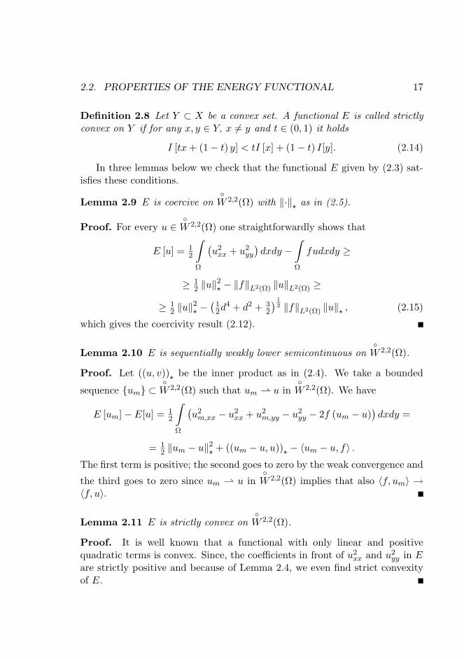
Definition 2.8 Let Y ⊂ X be a convex set. A functional E is called strictlyconvex on Y if for any x, y ∈ Y, x 6= y and t ∈ (0, 1) it holds
I [tx+ (1− t) y] < tI [x] + (1− t) I[y]. (2.14)
In three lemmas below we check that the functional E given by (2.3) sat-isfies these conditions.
Lemma 2.9 E is coercive onW 2,2(Ω) with ‖·‖? as in (2.5).
Proof. For every u ∈W 2,2(Ω) one straightforwardly shows that
E [u] = 12
∫Ω
(u2xx + u2
yy
)dxdy −
∫Ω
fudxdy ≥
≥ 12 ‖u‖
2? − ‖f‖L2(Ω) ‖u‖L2(Ω) ≥
≥ 12 ‖u‖
2? −
(12d
4 + d2 + 32
) 12 ‖f‖L2(Ω) ‖u‖? , (2.15)
which gives the coercivity result (2.12).
Lemma 2.10 E is sequentially weakly lower semicontinuous onW 2,2(Ω).
Proof. Let ((u, v))? be the inner product as in (2.4). We take a bounded
sequence um ⊂W 2,2(Ω) such that um u in
W 2,2(Ω). We have
E [um]− E[u] = 12
∫Ω
(u2m,xx − u2
xx + u2m,yy − u2
yy − 2f (um − u))dxdy =
= 12 ‖um − u‖2? + ((um − u, u))? − 〈um − u, f〉 .
The first term is positive; the second goes to zero by the weak convergence and
the third goes to zero since um u inW 2,2(Ω) implies that also 〈f, um〉 →
〈f, u〉.
Lemma 2.11 E is strictly convex onW 2,2(Ω).
Proof. It is well known that a functional with only linear and positivequadratic terms is convex. Since, the coefficients in front of u2
xx and u2yy in E
are strictly positive and because of Lemma 2.4, we even find strict convexityof E.
18 CHAPTER 2. EXISTENCE AND UNIQUENESS
2.3 Weak solution, existence and uniqueness result
The following statement holds.
Theorem 2.12 Suppose f ∈ L2(Ω). Then a weak solution of the boundaryvalue problem (1.4) in the sense of Definition 2.2 exists. Moreover, this solu-tion is unique.
Proof. The proof basically recalls the variational approach outlined in thebeginning of this Chapter. More precisely, by Lemmas 2.9 – 2.11 it followsthat
E [u] =∫Ω
(12
(u2xx + u2
yy
)− fu
)dxdy over
W 2,2(Ω),
is coercive, weakly lower semicontinuous and strictly convex on the spaceW 2,2(Ω). Due to the coercivity and the weak lower semicontinuity of E, thedirect method in the calculus of variations (see e.g. [6]) shows us that E has
a minimizer u ∈W 2,2(Ω). Due to strict convexity of E the minimizer u is
unique. For this u it holds that ddεE [u+ εϕ]
∣∣ε=0
= 0 for all ϕ ∈W 2,2(Ω).
The expansion of the latter condition results in (2.2), meaning that u is aweak solution of (1.4). Since a weak solution is a critical point of the given Eand since the critical point is unique, so is the weak solution.
Remark 2.13 For u ∈W 2,2(Ω) we have just shown that
‖u‖2W 2,2(Ω) ≤ C
∫Ω
(u2xx + u2
yy
)dxdy.
Let the grid be hinged, that is u ∈W 2,2(Ω)∩W 1,2(Ω). For every u ∈ C2(Ω)∩
C0(Ω) a Poincare inequality still yields (2.9) and (2.10). Indeed, due to u =0 on ∂Ω one find for every line y = c intersecting Ω that there is xc with(xc, c) ∈ Ω such that ux(xc, c) = 0. Starting from this point one proves (2.9)and similarly (2.10). Using a density argument (see e.g [22, page 171]) results
in the estimates above for every u ∈ W 2,2(Ω) ∩W 1,2(Ω). The real problem
is∫Ω
u2xydxdy since estimate (2.11) does not hold on domains with non-convex
corners.

Chapter 3
Homogeneous problem in aninfinite cone
As soon as we have the weak solution u ∈W 2,2(Ω) to the boundary value
problem (1.4) at hand we may improve its regularity.This chapter provides all the necessary information on the local behaviour
of u ∈W 2,2(Ω) in the vicinity of angular point 0 of Ω. This behaviour is
defined by the solutions of the homogeneous problemuxxxx + uyyyy = 0 in K(α,ω),
u = 0 on ∂K(α,ω),
∂∂nu = 0 on ∂K(α,ω)\0,
(3.1)
where K(α,ω) is an infinite cone defined in (1.5) and sketched in Figure 3.1.We derive almost explicit formulas for power type solutions to (3.1) and this
will enable us to see their contribution to the regularity of u ∈W 2,2(Ω) in
Chapter 5.
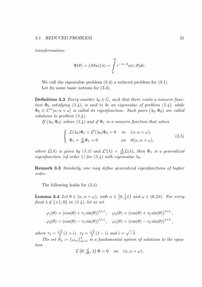
3.1 Reduced problem
The reduced problem for (3.1) is obtained in the following way. By Kondratiev[18] one should consider the power type solutions of (3.1):
u = rλ+1Φ(θ), (3.2)
19

20 CHAPTER 3. HOMOGENEOUS PROBLEM IN AN INFINITE CONE
(α,ω)
0
y
x
Κ
ω α
Figure 3.1: An infinite cone K(α,ω).
with x = r cos(θ) and y = r sin(θ). Here λ ∈ C and Φ : [α, α+ ω] → R.We insert u from (3.2) into problem (3.1) and find(
∂4
∂x4 + ∂4
∂y4
)(rλ+1Φ(θ)
)= rλ−3L
(θ, ddθ , λ
)Φ(θ),
with
L(θ, ddθ , λ
)= 3
4
(1 + 1
3 cos(4θ))d4
dθ4+ (λ− 2) sin(4θ) d
3
dθ3+
+32
(λ2 − 1−
(λ2 − 4λ− 7
3
)cos(4θ)
)d2
dθ2+
+(−λ3 + 6λ2 − 7λ− 2
)sin(4θ) ddθ +
+34
(λ4 − 2λ2 + 1 + 1
3
(λ4 − 8λ3 + 14λ2 + 8λ− 15
)cos(4θ)
).
(3.3)
Then we obtain a λ-dependent boundary value problem for Φ:L(θ, ddθ , λ
)Φ = 0 in (α, α+ ω),
Φ = ddθΦ = 0 on ∂(α, α+ ω).
(3.4)
Remark 3.1 The nonlinear eigenvalue problem (3.4) appears by a Mellin
3.1. REDUCED PROBLEM 21
transformation:
Φ(θ) = (Mu)(λ) =
∞∫0
r−λ−2u(r, θ)dr.
We call the eigenvalue problem (3.4) a reduced problem for (3.1).Let fix some basic notions for (3.4).
Definition 3.2 Every number λ0 ∈ C, such that there exists a nonzero func-tion Φ0 satisfying (3.4), is said to be an eigenvalue of problem (3.4), whileΦ0 ∈ C4 [α, α+ ω] is called its eigenfunction. Such pairs (λ0,Φ0) are calledsolutions to problem (3.4).
If (λ0,Φ0) solves (3.4) and if Φ1 is a nonzero function that solvesL(λ0)Φ1 + L′(λ0)Φ0 = 0 in (α, α+ ω),
Φ1 = ddθΦ1 = 0 on ∂(α, α+ ω),
(3.5)
where L(λ) is given by (3.3) and L′(λ) = ddλL(λ), then Φ1 is a generalized
eigenfunction (of order 1) for (3.4) with eigenvalue λ0.
Remark 3.3 Similarly, one may define generalized eigenfunctions of higherorder.
The following holds for (3.4).
Lemma 3.4 Let θ ∈ (α, α + ω), with α ∈[0, 1
2π)
and ω ∈ (0, 2π]. For everyfixed λ /∈ ±1, 0 in (3.4), let us set
ϕ1(θ) = (cos(θ) + τ1 sin(θ))λ+1 , ϕ2(θ) = (cos(θ) + τ2 sin(θ))λ+1 ,
ϕ3(θ) = (cos(θ)− τ1 sin(θ))λ+1 , ϕ4(θ) = (cos(θ)− τ2 sin(θ))λ+1 ,
where τ1 =√
22 (1 + i) , τ2 =
√2
2 (1− i) and i =√−1.
The set Sλ := ϕm4m=1 is a fundamental system of solutions to the equa-tion
L(θ, ddθ , λ
)Φ = 0 on (α, α+ ω).

22 CHAPTER 3. HOMOGENEOUS PROBLEM IN AN INFINITE CONE
Proof. The derivation of ϕm, m = 1, ..., 4 in Sλ is rather technical and werefer to Appendix B. There we also compute the Wronskian:
W (ϕ1 (θ) , ϕ2 (θ) , ϕ3 (θ) , ϕ4 (θ)) =
= 16 (λ+ 1)3 λ2 (λ− 1)(cos4(θ) + sin4 (θ)
)λ−2.
It is non-zero on θ ∈ (α, α + ω), with α ∈[0, 1
2π)
and ω ∈ (0, 2π] except forλ ∈ ±1, 0. Hence, for every fixed λ /∈ ±1, 0 the set ϕm4m=1 consists offour linear independent functions on (α, α+ ω).
Lemma 3.5 In the particular cases λ ∈ ±1, 0 in (3.4), one finds the fol-lowing fundamental systems:
S−1 =
1, arctan (cos(2θ)) , arctanh(√
22 sin(2θ)
), ϕ4(θ)
,
S0 = sin(θ), cos(θ), ϕ3(θ), ϕ4(θ) ,S1 = 1, sin(2θ), cos(2θ), ϕ4(θ) ,
where the explicit formulas for ϕ4 ∈ S−1, ϕ3, ϕ4 ∈ S0 and ϕ4 ∈ S1 are givenin Appendix B.
Proof. The fundamental systems S−1, S0, S1 are given in Appendix B. Bystraightforward computations one finds that for every above Sλ, λ ∈ ±1, 0the corresponding Wronskian W is proportional to
(cos4(θ) + sin4 (θ)
)λ−2, λ ∈±1, 0 and hence is nonzero on θ ∈ (α, α + ω), with α ∈
[0, 1
2π)
and ω ∈(0, 2π].
In terms of the fundamental systems S we have Φ that solves L(θ, ∂∂θ , λ
)Φ =
0 as
Φ(θ) =4∑
m=1
bmϕm(θ),
where bm ∈ C. Inserting this expression into the boundary conditions of prob-lem (3.4), we find a homogeneous system of four equations in the unknownsbm4m=1 reading as
Ab :=
ϕ1 (α) ϕ2 (α) ϕ3 (α) ϕ4 (α)
ϕ′1 (α) ϕ′2 (α) ϕ′3 (α) ϕ′4 (α)
ϕ1 (α+ ω) ϕ2 (α+ ω) ϕ3 (α+ ω) ϕ4 (α+ ω)
ϕ′1 (α+ ω) ϕ′2 (α+ ω) ϕ′3 (α+ ω) ϕ′4 (α+ ω)
b1
b2
b3
b4
= 0,
3.1. REDUCED PROBLEM 23
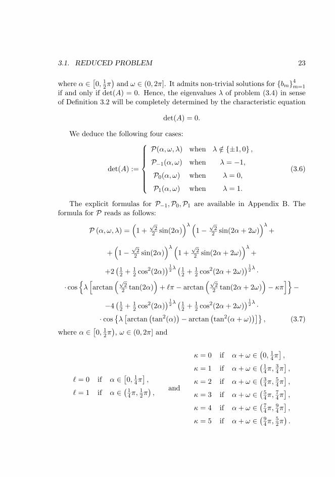
where α ∈[0, 1
2π)
and ω ∈ (0, 2π]. It admits non-trivial solutions for bm4m=1
if and only if det(A) = 0. Hence, the eigenvalues λ of problem (3.4) in senseof Definition 3.2 will be completely determined by the characteristic equation
det(A) = 0.
We deduce the following four cases:
det(A) :=
P(α, ω, λ) when λ /∈ ±1, 0 ,
P−1(α, ω) when λ = −1,
P0(α, ω) when λ = 0,
P1(α, ω) when λ = 1.
(3.6)
The explicit formulas for P−1,P0,P1 are available in Appendix B. Theformula for P reads as follows:
P (α, ω, λ) =(1 +
√2
2 sin(2α))λ (
1−√
22 sin(2α+ 2ω)
)λ+
+(1−
√2
2 sin(2α))λ (
1 +√
22 sin(2α+ 2ω)
)λ+
+2(
12 + 1
2 cos2(2α)) 1
2λ (1
2 + 12 cos2(2α+ 2ω)
) 12λ ·
· cosλ[arctan
(√2
2 tan(2α))
+ `π − arctan(√
22 tan(2α+ 2ω)
)− κπ
]−
−4(
12 + 1
2 cos2(2α)) 1
2λ (1
2 + 12 cos2(2α+ 2ω)
) 12λ ·
· cosλ[arctan
(tan2(α)
)− arctan
(tan2(α+ ω)
)], (3.7)
where α ∈[0, 1
2π), ω ∈ (0, 2π] and
` = 0 if α ∈[0, 1
4π],
` = 1 if α ∈(
14π,
12π),
and
κ = 0 if α+ ω ∈(0, 1
4π],
κ = 1 if α+ ω ∈(
14π,
34π],
κ = 2 if α+ ω ∈(
34π,
54π],
κ = 3 if α+ ω ∈(
54π,
74π],
κ = 4 if α+ ω ∈(
74π,
94π],
κ = 5 if α+ ω ∈(
94π,
52π).

24 CHAPTER 3. HOMOGENEOUS PROBLEM IN AN INFINITE CONE
Our purpose is to describe the eigenvalues λ of problem (3.4) for everyfixed α ∈
[0, 1
2π)
and fixed ω ∈ (0, 2π]. What is more important, we want totrace for a fixed α ∈
[0, 1
2π)
the behavior of ω 7→ λ(α, ω) on ω ∈ (0, 2π].The strategy will be as follows. First, we check for every α ∈
[0, 1
2π)
whether the equations P−1(α, ω) = 0, P0(α, ω) = 0 and P1(α, ω) = 0 haveany solutions in ω on the interval (0, 2π]. In this way we will see whetherλ ∈ ±1, 0 are eigenvalues of (3.4) or not. Next to this, we will address thetranscendental equation P(α, ω, λ) = 0. We will start from the basic propertyof the solutions λ to P(α, ω, λ) = 0 for fixed α ∈
[0, 1
2π)
and fixed ω ∈ (0, 2π]and then our detailed study will concern the equation P(α, ω, λ) = 0 withα = 0. In Section 3.3 we will describe the dependence of the eigenvalues λ onthe opening angle ω, particularly focusing on the eigenvalue with the lowestpositive real part, denoted as λ1. For this eigenvalue we prove the existenceof an interval of ω on which λ1 as a function of ω increases with increasing ω.
3.2 General statements for the eigenvalues λ
Let α ∈[0, 1
2π)
and ω ∈ (0, 2π] in problem (3.4). It holds that:
Lemma 3.6 For any α and ω the value λ = 0 is not an eigenvalue of (3.4).
Proof. The proof uses the fact that the function P0(α, ω) is strictly positiveon (α, ω) ∈
[0, 1
2π)× (0, 2π]. For details see Lemma B.1 in Appendix B.
Lemma 3.7 For all α ∈[0, 1
2π)
the values λ ∈ ±1 are eigenvalues of (3.4)when ω ∈ π, ω0, 2π, where ω0 ∈ (0, 2π).
Proof. It is straightforward that for every fixed α ∈[0, 1
2π)
the values ω ∈π, 2π are solutions to P−1(α, ω) = 0 and P1(α, ω) = 0 (see Appendix B). Onthe other hand, due to complexity of P−1 and P1 one is not able to find forevery fixed α the third solution ω0 ∈ (0, 2π) of P−1(α, ω) = 0 and P1(α, ω) = 0analytically. So, we have numerically assisted results. It turns out that bothforegoing equations for every fixed α have identical solutions, that we denoteas ω0. For instance, fixing α = 10
180πj, j = 0, ..., 8 we find the following
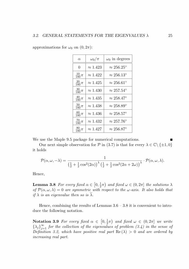
3.2. GENERAL STATEMENTS FOR THE EIGENVALUES λ 25
approximations for ω0 on (0, 2π):
α ω0/π ω0 in degrees
0 ≈ 1.423 ≈ 256.25
10180π ≈ 1.422 ≈ 256.13
20180π ≈ 1.425 ≈ 256.61
30180π ≈ 1.430 ≈ 257.54
40180π ≈ 1.435 ≈ 258.47
50180π ≈ 1.438 ≈ 258.89
60180π ≈ 1.436 ≈ 258.57
70180π ≈ 1.432 ≈ 257.76
80180π ≈ 1.427 ≈ 256.87
We use the Maple 9.5 package for numerical computations.Our next simple observation for P in (3.7) is that for every λ ∈ C\ ±1, 0
it holds
P(α, ω,−λ) =1(
12 + 1
2 cos2(2α))λ (1
2 + 12 cos2(2α+ 2ω)
)λ · P(α, ω, λ).
Hence,
Lemma 3.8 For every fixed α ∈[0, 1
2π)
and fixed ω ∈ (0, 2π] the solutions λof P(α, ω, λ) = 0 are symmetric with respect to the ω-axis. It also holds thatif λ is an eigenvalue then so is λ.
Hence, combining the results of Lemmas 3.6 – 3.8 it is convenient to intro-duce the following notation.
Notation 3.9 For every fixed α ∈[0, 1
2π)
and fixed ω ∈ (0, 2π] we writeλj∞j=1 for the collection of the eigenvalues of problem (3.4) in the sense ofDefinition 3.2, which have positive real part Re (λ) > 0 and are ordered byincreasing real part.
26 CHAPTER 3. HOMOGENEOUS PROBLEM IN AN INFINITE CONE
The complete set of eigenvalues to problem (3.4) will then read as −λj , λj∞j=1.The following lemma describes the set λj∞j=1.
Lemma 3.10 Let L be the operator given by (3.3).
• For every fixed α ∈[0, 1
2π)
and fixed ω ∈ (0, 2π]\ π, ω0, 2π the setλj∞j=1 from Notation 3.9 is given by
λj∞j=1 =λ ∈ C : Re (λ) ∈ R+\1, P(α, ω, λ) = 0
.
• For every fixed α ∈[0, 1
2π)
and fixed ω ∈ π, ω0, 2π the set λj∞j=1from Notation 3.9 is given by
λj∞j=1 =λ ∈ C : Re (λ) ∈ R+\1, P(α, ω, λ) = 0
∪ 1.
Here ω0 is a solution of P1(α, ω) = 0 on ω ∈ (π, 2π) for every fixed α ∈[0, 1
2π).
Remark 3.11 The approximations ω0/π for some fixed α are presented inthe table in the Proof of Lemma 3.7.
The last thing we can mention in this Section is that the values ω ∈12π, π,
32π, 2π
being set in (3.7) yield more simple formulas for P. We find
that:P(α, 1
2π, λ)
=(1−
√2
2 sin(2α))2λ
+(1 +
√2
2 sin(2α))2λ
+
+2(
12 + 1
2 cos2(2α))λ cos (λπ)−
− 4(
12 + 1
2 cos2(2α))λ cos
λ[arctan
(tan2(α)
)− arctan
(cot2(α)
)], (3.8)
P (α, π, λ) = −4(
12 + 1
2 cos2(2α))λ sin2(πλ), (3.9)
P(α, 3
2π, λ)
=(1−
√2
2 sin(2α))2λ
+(1 +
√2
2 sin(2α))2λ
+
+2(
12 + 1
2 cos2(2α))λ cos (3λπ)−
− 4(
12 + 1
2 cos2(2α))λ cos
λ[arctan
(tan2(α)
)− arctan
(cot2(α)
)], (3.10)

3.3. ANALYSIS OF THE EIGENVALUES λ WHEN α = 0 27
P (α, 2π, λ) = 16(
12 + 1
2 cos2(2α))λ [cos4(πλ)− cos2(πλ)
]. (3.11)
In the above formulas α ∈[0, 1
2π)
and λ /∈ ±1, 0. Equations P (α, π, λ) = 0and P (α, 2π, λ) = 0 admit the explicit solutions λ for every α ∈
[0, 1
2π), while
the equations P(α, 1
2π, λ)
= 0 and P(α, 3
2π, λ)
= 0 can be solved explicitlyonly for α = 0. For details see Appendix D.
3.3 Analysis of the eigenvalues λ when α = 0
The set λj∞j=1 of the eigenvalues to problem for every fixed α ∈[0, 1
2π)
and fixed ω ∈ (0, 2π] has been described by Lemma 3.10. In this Section ourparticular study will focus on λj∞j=1 when α = 0. First, we will give thebasic plot of some first values from λj∞j=1 in dependence on the openingangle ω ∈ (0, 2π]. This result is obtained in a numerically assisted way. Nextto this, a detailed numerically-analytical analysis will be given to λ1. We willprove that as a function of ω the first eigenvalue λ1 = λ1(ω) of the boundaryvalue problem (3.4) increases on ω ∈
(12π, ω?
), where ω?/π ≈ 0.528 (in degrees
ω? ≈ 95.1).Thus, we fix α = 0 in (3.7) and denote
P (ω, λ) := P(α, ω, λ)|α=0 .
Explicitly, P reads as follows:
P (ω, λ) =(1−
√2
2 sin(2ω))λ
+(1 +
√2
2 sin(2ω))λ
+
+2(
12 + 1
2 cos2(2ω)) 1
2λ · cos
λ[arctan
(√2
2 tan(2ω))
+ κπ]−
−4(
12 + 1
2 cos2(2ω)) 1
2λ · cos
λ arctan
(tan2(ω)
), (3.12)
and
κ = 0 if ω ∈(0, 1
4π],
κ = 1 if ω ∈(
14π,
34π],
κ = 2 if ω ∈(
34π,
54π],
κ = 3 if ω ∈(
54π,
74π],
κ = 4 if ω ∈(
74π, 2π
].

28 CHAPTER 3. HOMOGENEOUS PROBLEM IN AN INFINITE CONE
Now the particular case of Lemma 3.10 for the case α = 0 can be formulated.
Lemma 3.12 Let L be the operator given by (3.3) and let α = 0.
• For every fixed ω ∈ (0, 2π]\ π, ω0, 2π the set λj∞j=1 from Notation3.9 is given by
λj∞j=1 =λ ∈ C : Re (λ) ∈ R+\1, P (ω, λ) = 0
.
• For every fixed ω ∈ π, ω0, 2π the set λj∞j=1 from Notation 3.9 isgiven by
λj∞j=1 =λ ∈ C : Re (λ) ∈ R+\1, P (ω, λ) = 0
∪ 1.
Here ω0 is a solution of P1(α, ω) = 0|α=0 on ω ∈ (π, 2π) with the approx-imation ω0/π ≈ 1.424 (in degrees ω0 ≈ 256.25).
Also, referring to the formula (3.12), we will find:
P(
12π, λ
)= 2 + 2 cos(πλ)− 4 cos
(12πλ
),
P (π, λ) = −4 sin2(πλ),
P(
32π, λ
)= 8 cos3(πλ)− 6 cos(πλ)− 4 cos
(12πλ
)+ 2,
P (2π, λ) = 16 cos4(πλ)− 16 cos2(πλ).
In Appendix D we solve the above four equations explicitly.
3.3.1 Intermezzo: a comparison with ∆2
Let the grid-operator ∂4
∂x4 + ∂4
∂y4in problems (1.4), (3.1) be replaced by the
bilaplacian ∆2 = ∂4
∂x4 + 2 ∂4
∂x2∂y2+ ∂4
∂y4. That is, we have the clamped plate
problem, ∆2u = f in Ω,
u = 0 on ∂Ω,∂∂nu = 0 on ∂Ω\0,
(3.13)
“with prescribed growth behaviour near 0”,
3.3. ANALYSIS OF THE EIGENVALUES λ WHEN α = 0 29
and the homogeneous problem in an infinite cone,∆2u = 0 in K(α,ω),
u = 0 on ∂K(α,ω),
∂∂nu = 0 on ∂K(α,ω)\0.
(3.14)
Here, Ω and K(α,ω) are from Condition 1.2. Due to the invariance of theoperator ∆2 under rotation, the orientation angle α in problems (3.13) and(3.14) does not play a role, i.e. can be arbitrary. But in order to be consistentwith the particular case α = 0 in the grid problem we consider here, we simplyassume that α = 0 in the above bilaplacian problems too.
Here, we recall some results for the bilaplacian, namely, the eigenvaluesλj∞j=1 of the corresponding reduced problem. We will compare them tothose given in Lemma 3.12. For problem (3.14) the reduced problem of thetype (3.4) has an operator L reading as (see e.g. [14, page 88]):
L(θ, ddθ , λ
)= d4
dθ4+ 2
(λ2 + 1
)d2
dθ2+(λ4 − 2λ2 + 1
). (3.15)
The corresponding characteristic determinants are the following (see e.g. [14,page 89] or [3, page 561]):
det(A) :=
sin2(λω)− λ2 sin2(ω) when λ /∈ ±1, 0 ,
sin2(ω)− ω2 when λ = 0,
sin(ω) (sin(ω)− ω cos(ω)) when λ ∈ ±1 .
(3.16)
Note that for every λ ∈ C\ ±1, 0 the function sin2(λω) − λ2 sin2(ω) iseven with respect to ω and hence the Notation 3.9 is applicable here. Analysisof det(A) = 0 with det(A) as in (3.16) enables to formulate the analog ofLemma 3.12. Namely,
Lemma 3.13 Let L be the operator given by (3.15).
• For every fixed ω ∈ (0, 2π]\ π, ω0, 2π the set λj∞j=1 from Notation3.9 is given by
λj∞j=1 =λ ∈ C : Re (λ) ∈ R+\1, sin2(λω)− λ2 sin2(ω) = 0
.
30 CHAPTER 3. HOMOGENEOUS PROBLEM IN AN INFINITE CONE
• For every fixed ω ∈ π, ω0, 2π the set λj∞j=1 from Notation 3.9 isgiven by
λj∞j=1 =λ ∈ C : Re (λ) ∈ R+\1, sin2(λω)− λ2 sin2(ω) = 0
∪1.
Here ω0 is a solution of tan(ω) = ω on ω ∈ (π, 2π) with the approximationω0/π ≈ 1.430 (in degrees ω0 ≈ 257.45).
3.4 Analysis of the eigenvalues λ when α = 0 (con-tinued)
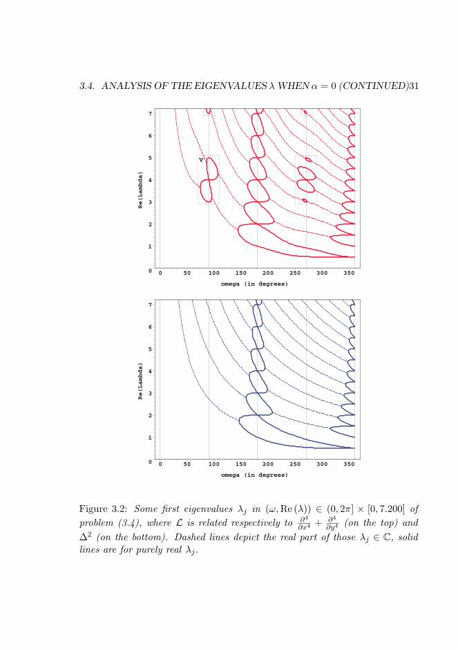
Let (ω, λ) be the pair that solves the equations of Lemmas 3.12 and 3.13.In Figure 3.2 we plot the pairs (ω,Re (λ)) inside the region (ω,Re (λ)) ∈(0; 2π]× [0, 7.200].
Remark 3.14 The numerical computations are performed with the Maple 9.5package in the following way: at a first cycle for every ωq = 21
180π + 160πq,
q = 0, ..., 113 we compute the entries of the set λjNj=1. Here, N is determinedby the condition: Re (λN ) ≤ 7.200 and Re (λN+1) > 7.200. The points (ω, λ)where λj transits from the complex plane to the real one or vice-versa aresolutions to the system P (ω, λ) = 0 and ∂P
∂λ (ω, λ) = 0 (the justification for thesecond condition will be discussed in Lemma 3.20).
In Figure 3.2 one may observe the difference in the behavior of the eigen-values in the corresponding cases. In particular, in the top plot (the caseL = ∂4
∂x4 + ∂4
∂y4) there are the “loops” and the “ellipses” in the vicinities of
ω ∈
12π,
32π
(we inclose them in the rectangles). The bottom plot (the caseL = ∆2) looks much simpler in the same region. We will see from the reg-ularity statements in Chapter 5 that the contribution of the first eigenvalueλ1 to the regularity of the solution u to problem (1.4) is the most essential.So, it is important for us to know the dependence of the eigenvalues λ on theopening angle ω. In this sense, the region (ω,Re (λ)) ∈ V (Figure 3.2, top)seems to be the most interesting part and the model one. One observes thatinside V the graph of the implicit function P (ω,λ) = 0 looks like a deformed8-shaped curve. So, if one proves that everywhere in V , P (ω,λ) = 0 allows itslocal parametrization in ω 7→ λ = ψ(ω) or λ 7→ ω = ϕ(λ), then the bottompart of this graph is λ1 and there is a subset of the this bottom part where λ1
as a function of ω increases with increasing ω.
3.4. ANALYSIS OF THE EIGENVALUES λWHEN α = 0 (CONTINUED)31
V
0
1
2
3
4
5
6
7
Re(Lambda)
0 50 100 150 200 250 300 350
omega (in degrees)
0
1
2
3
4
5
6
7
Re(Lambda)
0 50 100 150 200 250 300 350
omega (in degrees)
Figure 3.2: Some first eigenvalues λj in (ω,Re (λ)) ∈ (0, 2π] × [0, 7.200] ofproblem (3.4), where L is related respectively to ∂4
∂x4 + ∂4
∂y4(on the top) and
∆2 (on the bottom). Dashed lines depict the real part of those λj ∈ C, solidlines are for purely real λj .
32 CHAPTER 3. HOMOGENEOUS PROBLEM IN AN INFINITE CONE
3.4.1 Behavior of λ in V
So let us fix the open rectangular domain
V =(ω, λ) :
[70180π,
110180π
]× [2.900, 5.100]
.
The function P∈ C∞(V,R) is given by (3.12) with κ = 1:
P (ω, λ) =(1−
√2
2 sin(2ω))λ
+(1 +
√2
2 sin(2ω))λ
+
+2(
12 + 1
2 cos2(2ω)) 1
2λ · cos
λ[arctan
(√2
2 tan(2ω))
+ π]−
−4(
12 + 1
2 cos2(2ω)) 1
2λ · cos
λ arctan
(tan2(ω)
). (3.17)
We set
Γ:= (ω,λ) ∈ V : P (ω,λ) = 0, (3.18)
as a zero level set of P in V .
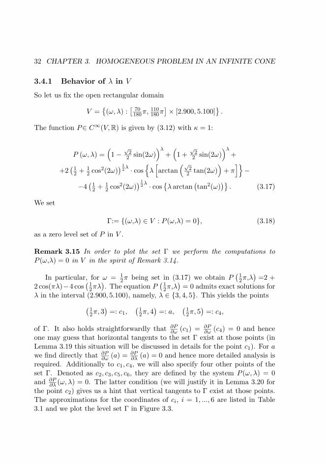
Remark 3.15 In order to plot the set Γ we perform the computations toP (ω,λ) = 0 in V in the spirit of Remark 3.14.
In particular, for ω = 12π being set in (3.17) we obtain P
(12π,λ
)=2 +
2 cos(πλ)−4 cos(
12πλ
). The equation P
(12π,λ
)= 0 admits exact solutions for
λ in the interval (2.900, 5.100), namely, λ ∈ 3, 4, 5. This yields the points(12π, 3
)=: c1,
(12π, 4
)=: a,
(12π, 5
)=: c4,
of Γ. It also holds straightforwardly that ∂P∂ω (c1) = ∂P
∂ω (c4) = 0 and henceone may guess that horizontal tangents to the set Γ exist at those points (inLemma 3.19 this situation will be discussed in details for the point c1). For awe find directly that ∂P
∂ω (a) = ∂P∂λ (a) = 0 and hence more detailed analysis is
required. Additionally to c1, c4, we will also specify four other points of theset Γ. Denoted as c2, c3, c5, c6, they are defined by the system P (ω, λ) = 0and ∂P
∂λ (ω, λ) = 0. The latter condition (we will justify it in Lemma 3.20 forthe point c2) gives us a hint that vertical tangents to Γ exist at those points.The approximations for the coordinates of ci, i = 1, ..., 6 are listed in Table3.1 and we plot the level set Γ in Figure 3.3.
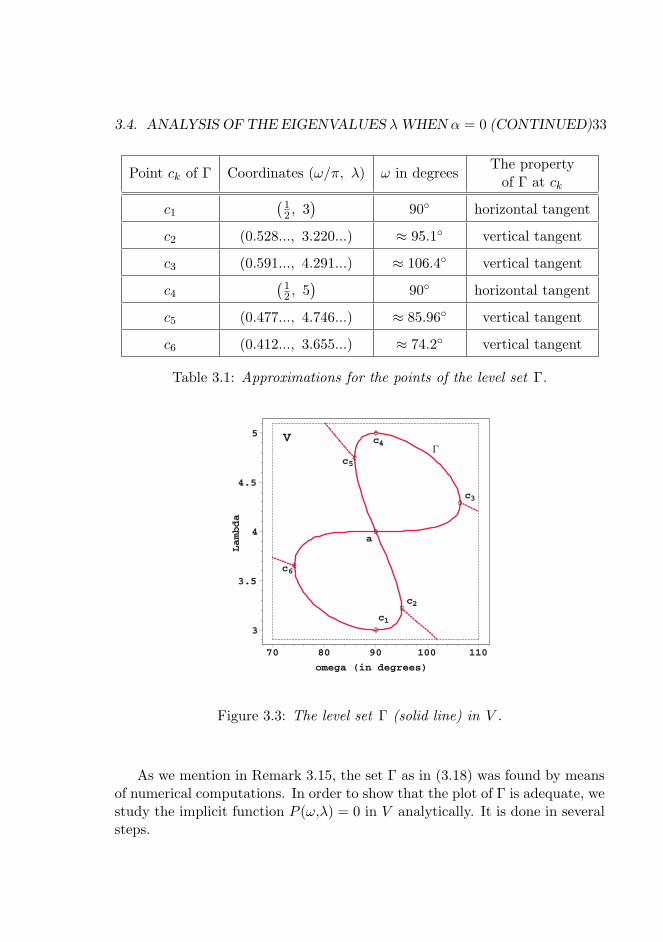
3.4. ANALYSIS OF THE EIGENVALUES λWHEN α = 0 (CONTINUED)33
Point ck of Γ Coordinates (ω/π, λ) ω in degreesThe property
of Γ at ck
c1(
12 , 3
)90 horizontal tangent
c2 (0.528..., 3.220...) ≈ 95.1 vertical tangent
c3 (0.591..., 4.291...) ≈ 106.4 vertical tangent
c4(
12 , 5
)90 horizontal tangent
c5 (0.477..., 4.746...) ≈ 85.96 vertical tangent
c6 (0.412..., 3.655...) ≈ 74.2 vertical tangent
Table 3.1: Approximations for the points of the level set Γ.
ΓV
6c
5c
4c
3c
2c
1c
a
3
3.5
4
4.5
5
Lambda
70 80 90 100 110
omega (in degrees)
Figure 3.3: The level set Γ (solid line) in V .
As we mention in Remark 3.15, the set Γ as in (3.18) was found by meansof numerical computations. In order to show that the plot of Γ is adequate, westudy the implicit function P (ω,λ) = 0 in V analytically. It is done in severalsteps.
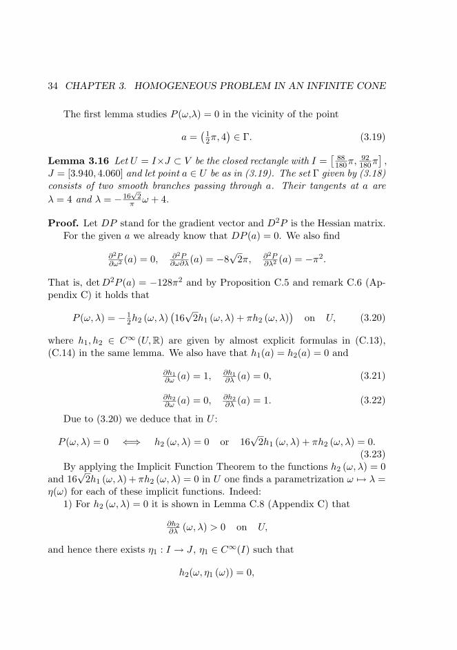
34 CHAPTER 3. HOMOGENEOUS PROBLEM IN AN INFINITE CONE
The first lemma studies P (ω,λ) = 0 in the vicinity of the point
a =(
12π, 4
)∈ Γ. (3.19)
Lemma 3.16 Let U = I×J ⊂ V be the closed rectangle with I =[
88180π,
92180π
],
J = [3.940, 4.060] and let point a ∈ U be as in (3.19). The set Γ given by (3.18)consists of two smooth branches passing through a. Their tangents at a areλ = 4 and λ = −16
√2
π ω + 4.
Proof. Let DP stand for the gradient vector and D2P is the Hessian matrix.For the given a we already know that DP (a) = 0. We also find
∂2P∂ω2 (a) = 0, ∂2P
∂ω∂λ(a) = −8√
2π, ∂2P∂λ2 (a) = −π2.
That is, detD2P (a) = −128π2 and by Proposition C.5 and remark C.6 (Ap-pendix C) it holds that
P (ω, λ) = −12h2 (ω, λ)
(16√
2h1 (ω, λ) + πh2 (ω, λ))
on U, (3.20)
where h1, h2 ∈ C∞ (U,R) are given by almost explicit formulas in (C.13),(C.14) in the same lemma. We also have that h1(a) = h2(a) = 0 and
∂h1∂ω (a) = 1, ∂h1
∂λ (a) = 0, (3.21)
∂h2∂ω (a) = 0, ∂h2
∂λ (a) = 1. (3.22)
Due to (3.20) we deduce that in U :
P (ω, λ) = 0 ⇐⇒ h2 (ω, λ) = 0 or 16√
2h1 (ω, λ) + πh2 (ω, λ) = 0.(3.23)
By applying the Implicit Function Theorem to the functions h2 (ω, λ) = 0and 16
√2h1 (ω, λ) + πh2 (ω, λ) = 0 in U one finds a parametrization ω 7→ λ =
η(ω) for each of these implicit functions. Indeed:1) For h2 (ω, λ) = 0 it is shown in Lemma C.8 (Appendix C) that
∂h2∂λ (ω, λ) > 0 on U,
and hence there exists η1 : I → J , η1 ∈ C∞(I) such that
h2(ω, η1 (ω)) = 0,
3.4. ANALYSIS OF THE EIGENVALUES λWHEN α = 0 (CONTINUED)35
andη′1 (ω) = −∂h2
∂ω (ω, η1 (ω))[∂h2∂λ (ω, η1 (ω))
]−1,
for all ω ∈ I. We have that η1
(12π)
= 4 and due to (3.22) we find
η′1(
12π)
= 0.
Hence, there is a smooth branch of Γ in U passing through a, which isgiven by λ = η1 (ω) with the tangent λ = 4.
2) For 16√
2h1 (ω, λ)+πh2 (ω, λ) = 0 it is shown in Lemma C.9 (AppendixC) that
16√
2∂h1∂λ (ω, λ) + π ∂h2
∂λ (ω, λ) > 0 on U,
and hence there exists η2 : I → J , η2 ∈ C∞(I), where I ⊂ I, such that
16√
2h1 (ω, η2 (ω)) + πh2 (ω, η2 (ω)) = 0,
and
η′2 (ω) = −16√
2∂h1∂ω (ω, η2 (ω)) + π ∂h2
∂ω (ω, η2 (ω))
16√
2∂h1∂λ (ω, η2 (ω)) + π ∂h2
∂λ (ω, η2 (ω)),
for all ω ∈ I. We have that η2
(12π)
= 4 and due to (3.21) and (3.22) we obtain
η′2(
12π)
= −16√
2π .
Hence, there is another smooth branch of Γ in U passing through a andgiven by λ = η2 (ω). The tangent is λ = −16
√2
π ω + 4.The next lemma studies P (ω,λ) = 0 locally in V but away from the point
a.
Lemma 3.17 Let
H1 =(ω, λ) :
[84180π,
90180π
]× [4.030, 4.970]
,
H2 =(ω, λ) :
[87180π,
101180π
]× [4.750, 5.100]
,
H3 =(ω, λ) :
[100180π,
108180π
]× [4.000, 4.850]
,
H4 =(ω, λ) :
[91180π,
102180π
]× [3.950, 4.100]
,
H5 =(ω, λ) :
[90180π,
96180π
]× [3.030, 3.970]
,
H6 =(ω, λ) :
[79180π,
94180π
]× [2.900, 3.230]
,
36 CHAPTER 3. HOMOGENEOUS PROBLEM IN AN INFINITE CONE
H7 =(ω, λ) :
[72180π,
80180π
]× [3.150, 4.000]
,
H8 =(ω, λ) :
[78180π,
89180π
]× [3.900, 4.050]
,
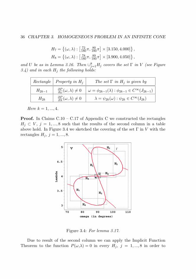
and U be as in Lemma 3.16. Then ∪8j=1Hj covers the set Γ in V (see Figure
3.4) and in each Hj the following holds:
Rectangle Property in Hj The set Γ in Hj is given by
H2k−1∂P∂ω (ω, λ) 6= 0 ω = φ2k−1(λ) : φ2k−1 ∈ C∞(J2k−1)
H2k∂P∂λ (ω, λ) 6= 0 λ = ψ2k(ω) : ψ2k ∈ C∞(I2k)
Here k = 1, ..., 4.
Proof. In Claims C.10 – C.17 of Appendix C we constructed the rectanglesHj ⊂ V , j = 1, ..., 8 such that the results of the second column in a tableabove hold. In Figure 3.4 we sketched the covering of the set Γ in V with therectangles Hj , j = 1, ..., 8.
ΓV
a8H
7H
6H
5H
4H
3H
2H
1H
U
3
3.5
4
4.5
5
Lambda
70 80 90 100 110
omega (in degrees)
Figure 3.4: For lemma 3.17.
Due to result of the second column we can apply the Implicit FunctionTheorem to the function P (ω,λ) = 0 in every Hj , j = 1, ..., 8 in order to
3.4. ANALYSIS OF THE EIGENVALUES λWHEN α = 0 (CONTINUED)37
obtain ω = φ2k−1(λ) or λ= ψ2k(ω), k = 1, ..., 4. By assumption P∈ C∞(V,R)and hence φ, ψ are C∞ on the corresponding intervals J, I.
Basing on the results of the above two lemmas we arrive at the following
Proposition 3.18 The set Γ given by (3.18) is an 8-shaped curve. That is,there exists an open set V ⊃ [−1, 1]2 and a C∞-diffeomorphism S : V → Vsuch that
S (Γ) = (sin(2t), sin(t)), 0 ≤ t < 2π .
Henceforth, we will call the set Γ a curve (having one self-intersectionpoint) which means that every part of the set Γ is locally parametrizable in ωor λ.
3.4.2 Eigenvalue λ1 as the bottom part of Γ
The curve Γ in a rectangle V combines the graphs of the first four eigenvaluesλ1, ..., λ4 of the boundary value problem (3.4) as functions of ω as far asthey are real. Here we focus on the eigenvalue λ1 which is a bottom part ofΓ (the segment c6c1c2 ⊂ Γ in Figure 3.3). In particular, we prove that as afunction of ω the eigenvalue λ1 = λ1(ω) increases between the points c1, c2 (theapproximations for their coordinates are given in Table 3.1). The situation isillustrated by Figure 3.5.
In order to prove this result, we follow the approach used in Lemmas 3.16and 3.17. To be more precise, we fix two rectangles H0,H? ⊂ V suchthat H0 ∩ H? = ∅ and H0 ∪ H? covers the part of Γ containing the seg-ment c1c2 (see Figure 3.6). We parameterize Γ in H0,H? as ω 7→ λ = ψ(ω)and λ 7→ ω = ϕ(λ), respectively, and study the properties of these para-metrizations (convexity-concavity, extremum points, the intervals of increase-decrease). This will enable to gain the information about c1c2.
Lemma 3.19 Let H0 = I0 × J0 ⊂ V be the closed rectangle with I0 =[84180π,
94180π
]and J0 = [2.960, 3.060]. It holds that Γ in H0 is given by λ =
ψ(ω), ψ ∈ C∞(ωα, ωβ), (ωα, ωβ) ⊂ I0 and is such that it attains its minimumon (ωα, ωβ) at ω = ω0 = 1
2π and increases monotonically on (ω0, ωβ). Hereωα, ωβ are the solutions to the equation P (ω, 3.060) = 0 on ω ∈
(84180π,
12π)
and on ω ∈(
12π,
94180π
), respectively, with P given by (3.17).
Proof. By Lemma 3.17 we know that
P (ω, λ) = 0 ⇐⇒ P (ω, ψ (ω)) = 0 in H6, (3.24)

38 CHAPTER 3. HOMOGENEOUS PROBLEM IN AN INFINITE CONE
VΓ
2c
1c
3
3.5
4
4.5
5
Lambda
70 80 90 100 110
omega (in degrees)
Figure 3.5: Increase of λ1 between c1 and c2
and if we take the rectangle H0 defined as in lemma above, then due to H0 ⊂H6, (3.24) will also hold in H0. Moreover, we also set H0 in such a way that itstop boundary intersects Γ at two points, meaning that we find two solutionsof P (ω, 3.060) = 0 with P as in (3.17). We name these two solutions ωα, ωβ.
Hence, we deduce that Γ in H0 is given by λ = ψ(ω), ψ ∈ C∞(ωα, ωβ) andsatisfies ψ(ωα) = ψ(ωβ) = 3.060. Due to condition
ψ(ωα) = ψ(ωβ),
by Rolle’s theorem there exists ω0 ∈ (ωα, ωβ) such that ψ′(ω0) = 0.Since P (ω0, ψ (ω0)) = 0 and due to
ψ′(ω) = −∂P∂ω (ω, ψ (ω))
[∂P∂λ (ω, ψ (ω))
]−1,
we solve the system P (ω, λ) = 0 and ∂P∂ω (ω, λ) = 0 in H0 in order to find ω0.
Its solution is a point c1 =(
12π, 3
)and hence
ω0 = 12π.
We deduce that λ = ψ(ω) attains its local extremum at ω = ω0.

3.4. ANALYSIS OF THE EIGENVALUES λWHEN α = 0 (CONTINUED)39
ΓV
0H
*H
3
3.5
4
4.5
5
Lambda
70 80 90 100 110
omega (in degrees)
0H
*H
3
3.1
3.2
3.3
3.4
3.5
3.6
Lambda
84 86 88 90 92 94 96
omega (in degrees)
Figure 3.6: The rectangles H0,H? from lemmas 3.19 and 3.20, respectively(on the left); the enlarged view (on the right).
Next we show that λ = ψ(ω) has a minimum at ω = ω0 on (ωα, ωβ). Forthis purpose we consider a function G ∈ C∞ (H0,R) such that
G (ω, ψ(ω)) = ψ′′(ω). (3.25)
40 CHAPTER 3. HOMOGENEOUS PROBLEM IN AN INFINITE CONE
For an explicit formula for G see Appendix C. In Claim C.18 of this Appendixwe show that
G (ω, λ) > 0 on H0. (3.26)
Condition (3.26) together with (3.25) yields
G (ω, ψ(ω)) = ψ′′(ω) > 0 on (ωα, ωβ),
meaning that λ = ψ(ω) is convex on (ωα, ωβ).The result is that λ = ψ(ω) attains its minimum on (ωα, ωβ) at ω = ω0 =
12π and increases monotonically on the interval ω ∈ (ω0, ωβ).
We also have the following
Lemma 3.20 Let H? = I? × J? ⊂ V be the closed rectangle with I? =[93.5180 π,
95.5180 π
]and J? = [3.030, 3.600]. It holds that Γ in H? is given by
ω = ϕ(λ), ϕ ∈ C∞(λγ , λδ), (λγ , λδ) ⊂ J? and is such that it attains itsmaximum on (λγ , λδ) at λ = λ? ≈ 3.220 and increases monotonically on theinterval (λγ , λ?). Here λγ , λδ are the solutions to the equation P
(93.5180 π, λ
)= 0
on λ ∈ (3.030, 3.100) and on λ ∈ (3.500, 3.600), respectively. Also, λ? is thesolution to the system P (ω, λ) = 0 and ∂P
∂λ (ω, λ) = 0 on λ ∈ (λγ , λδ); P givenby (3.17).
Proof. By Lemma 3.17 we know that
P (ω, λ) = 0 ⇐⇒ P (ϕ(λ), λ) = 0 in H5, (3.27)
and if we take the rectangle H? defined as in lemma above, then due to H? ⊂H5, (3.27) will also hold in H?. Moreover, we also set H? in such a way thatits left boundary intersects Γ at two points, meaning we find two solutions ofP(
93.5180 π, λ
)= 0 with P as in (3.17). We name these two solutions λγ , λδ.
Hence, we deduce that Γ in H? is given by ω = ϕ(λ), ϕ ∈ C∞(λγ , λδ) andsatisfies ϕ(λγ) = ϕ(λδ) = 93.5
180 π. Due to condition
ϕ(λγ) = ϕ(λδ),
by Rolle’s theorem there exists λ? ∈ (λγ , λδ) such that ϕ′(λ?) = 0.Since P (ϕ(λ?), λ?) = 0 and due to
ϕ′(λ) = −∂P∂λ (ϕ(λ), λ)
[∂P∂ω (ϕ(λ), λ)
]−1,

3.5. ON THE BEHAVIOUR OF ω 7→ λ1(ω), ω ∈ (0, 2π] WHEN α ∈(0, 1
2π)41
we solve the system P (ω, λ) = 0 and ∂P∂λ (ω, λ) = 0 in H? in order to find λ?.
Its solution is a point c2 =(ω, λ
), where ω/π ≈ 0.528and λ ≈ 3.220. Hence,
λ? ≈ 3.220.
We deduce that ω = ϕ(λ) attains its local extremum at λ = λ?.Next we show that ω = ϕ(λ) has a maximum at λ = λ? on (λγ , λδ). For
this purpose we consider a function F ∈ C∞ (H?,R) such that
F (ϕ(λ), λ) = ϕ′′(λ). (3.28)
For explicit formula for F see Appendix C. In Claim C.19 of this Appendixwe show that
F (ω, λ) < 0 on H?. (3.29)
Condition (3.29) together with (3.28) yields
F (ϕ(λ), λ) = ϕ′′(λ) < 0 on (λγ , λδ),
meaning that ω = ϕ(λ) is concave on (λγ , λδ).The result is that ω = ϕ(λ) attains its maximum on (λγ , λδ) at λ = λ? ≈
3.220 and increases monotonically on the interval λ ∈ (λγ , λ?).
Theorem 3.21 As a function of ω the first eigenvalue λ1 = λ1(ω) of theboundary value problem (3.4) increases on ω ∈
(12π, ω?
). Here ω?/π ≈ 0.528
(in degrees ω? ≈ 95.1).
3.5 On the behaviour of ω 7→ λ1(ω), ω ∈ (0, 2π] whenα ∈
(0, 1
2π)
The previous section has studied the eigenvalue λ1 of problem (3.4) on ω ∈(0, 2π], when α = 0 and described ω 7→ λ1(ω). Here we will give an impressionabout the behaviour of λ1 of (3.4) on ω ∈ (0, 2π], when α ∈
(0, 1
2π). In
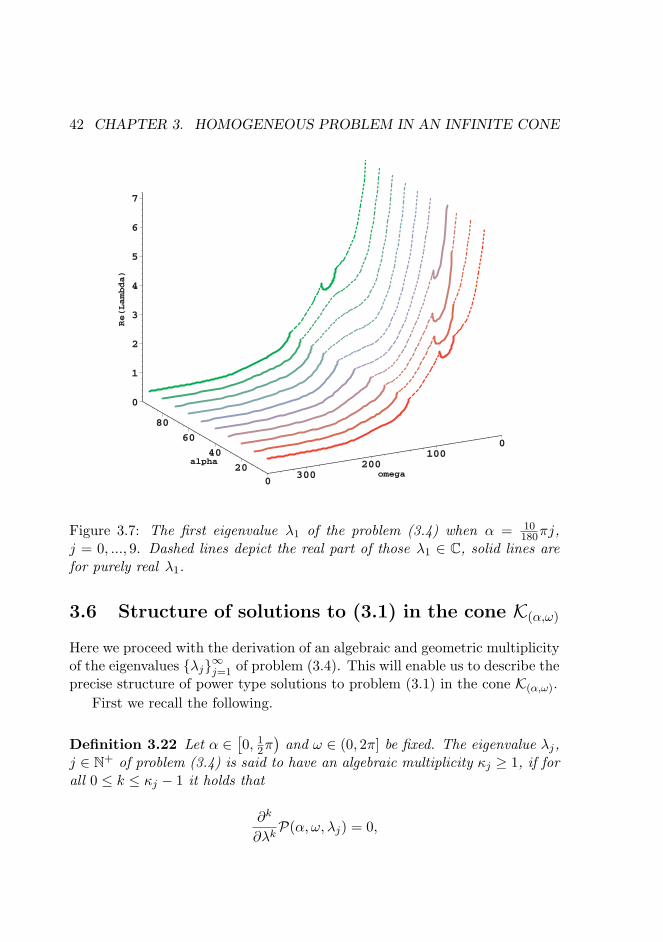
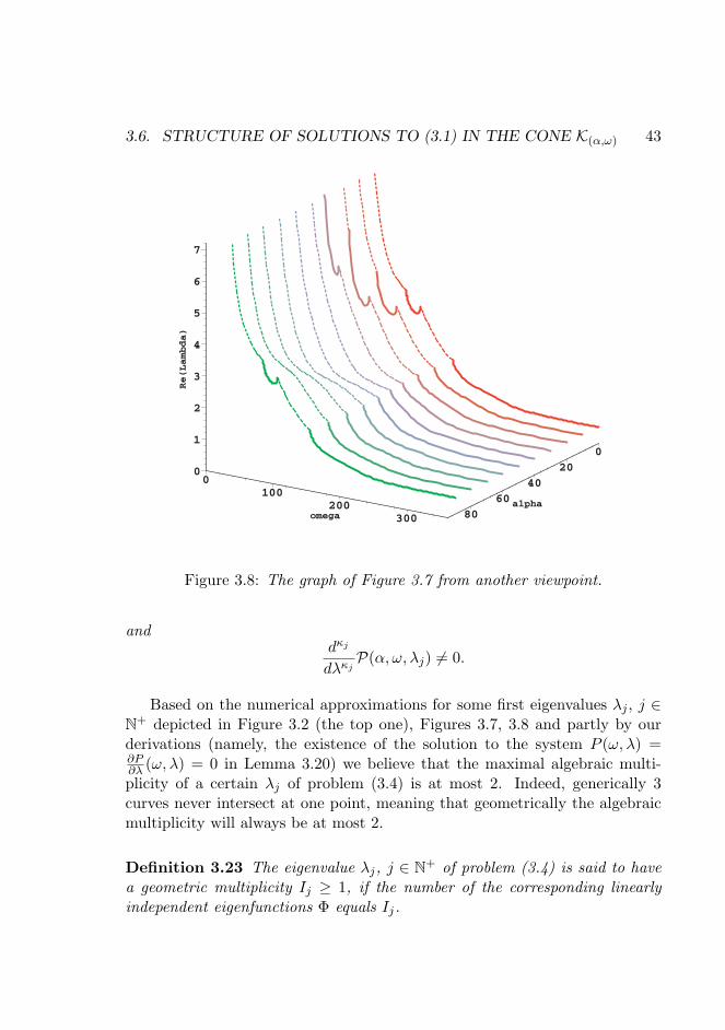
Figures 3.7 and 3.8, which are the same plots viewed from different viewpoints,we depict the eigenvalue λ1 of (3.4) for α = 10
180πj, j = 0, ..., 8. Note, thatalthough the case α = 1
2π is identical to the case α = 0 we, however, plot thecorresponding curve (the one in green) in order to complete the row.
42 CHAPTER 3. HOMOGENEOUS PROBLEM IN AN INFINITE CONE
020
40
60
80
alpha
0100
200300 omega
0
1
2
3
4
5
6
7
Re(Lambda)
Figure 3.7: The first eigenvalue λ1 of the problem (3.4) when α = 10180πj,
j = 0, ..., 9. Dashed lines depict the real part of those λ1 ∈ C, solid lines arefor purely real λ1.
3.6 Structure of solutions to (3.1) in the cone K(α,ω)
Here we proceed with the derivation of an algebraic and geometric multiplicityof the eigenvalues λj∞j=1 of problem (3.4). This will enable us to describe theprecise structure of power type solutions to problem (3.1) in the cone K(α,ω).
First we recall the following.
Definition 3.22 Let α ∈[0, 1
2π)
and ω ∈ (0, 2π] be fixed. The eigenvalue λj,j ∈ N+ of problem (3.4) is said to have an algebraic multiplicity κj ≥ 1, if forall 0 ≤ k ≤ κj − 1 it holds that
∂k
∂λkP(α, ω, λj) = 0,
3.6. STRUCTURE OF SOLUTIONS TO (3.1) IN THE CONE K(α,ω) 43
0
20
4060
80alpha
0100
200300omega
0
1
2
3
4
5
6
7
Re(Lambda)
Figure 3.8: The graph of Figure 3.7 from another viewpoint.
anddκj
dλκjP(α, ω, λj) 6= 0.
Based on the numerical approximations for some first eigenvalues λj , j ∈N+ depicted in Figure 3.2 (the top one), Figures 3.7, 3.8 and partly by ourderivations (namely, the existence of the solution to the system P (ω, λ) =∂P∂λ (ω, λ) = 0 in Lemma 3.20) we believe that the maximal algebraic multi-plicity of a certain λj of problem (3.4) is at most 2. Indeed, generically 3curves never intersect at one point, meaning that geometrically the algebraicmultiplicity will always be at most 2.
Definition 3.23 The eigenvalue λj, j ∈ N+ of problem (3.4) is said to havea geometric multiplicity Ij ≥ 1, if the number of the corresponding linearlyindependent eigenfunctions Φ equals Ij.

44 CHAPTER 3. HOMOGENEOUS PROBLEM IN AN INFINITE CONE
For given λj , j ∈ N+ of problem (3.4) we distinguish the following threecases:
1. κj = Ij = 1 one finds a solution (λj ,Φj,0) of (3.4) and then the powertype solution of problem (3.1) reads:
uj,0 = rλj+1Φj,0(θ); (3.30)
2. κj = 2, Ij = 1 one finds a solution (λj ,Φj,0) and a generalized solution(λj ,Φj,1) of (3.4). Recall that (λj ,Φj,1) satisfies the equation (3.5),
L(λj)Φj,1 + L′(λj)Φj,0 = 0,
where L(λ) is given by (3.3) and L′(λ) = ddλL(λ).
Then we have two solutions of problem (3.1):
uj,0 = rλj+1Φj,0(θ) and uj,1 = rλj+1 (Φj,1(θ) + log(r)Φj,0(θ)) ; (3.31)
3. κj = Ij = 2 one finds two solutions (λj ,Φj,0), (λj ,Φj,1) of (3.4), whereΦj,0 and Φj,1 are linearly independent on θ ∈ (α, α+ ω). Then as in previouscase, the two solutions of problem (3.1) occur:
uj,0 = rλj+1Φj,0(θ) and uj,1 = rλj+1Φj,1(θ). (3.32)
For our grid operator, in some cases of α and ω one is able to find theeigenvalues λj∞j of problem (3.4) explicitly. This happens when
α = 0 ω = 12π,
α ∈[0, 1
2π)
ω = π,
α = 0 ω = 32π,
α ∈[0, 1
2π)
ω = 2π.
Moreover,
• when α = 0 and the opening angle ω ∈
12π, π
, for every given λj
one can compute explicitly the corresponding eigenfunctions Φj,q, q =0, ..., κj − 1. If ω ∈
32π, 2π
, the eigenfunctions Φj,q can be computed
explicitly only for some λj . In Appendix D we bring the formulas of somefirst solutions uj,q to (3.1) for the corresponding cases (if computable);

3.6. STRUCTURE OF SOLUTIONS TO (3.1) IN THE CONE K(α,ω) 45
• when α ∈(0, 1
2π)
and the opening angle ω = π the first eigenvalues ofproblem (3.4) is λ1 = 1. Then one computes Φ1,0(θ) = sin2(θ−α) whichyields u1,0 = r2 sin2(θ−α). For higher values λj , j ≥ 2 the solutions uj,qare polynomials.
These functions rλ+1Φ(θ) and rλ+1 log(r)Φ(θ) determine the bands for theregularity in Kondratiev’s theory. Details are found in Chapter 5.

Chapter 4
Kondratiev’s weightedSobolev spaces
Due to Kondratiev [18], one of the appropriate functional spaces for the bound-ary value problems of the type (1.4) are the weighted Sobolev spaces V l,2
β ,where l ∈ 0, 1, 2, . . . and β ∈ R. Such spaces can be defined in differentways: either via the set of the square-integrable weighted weak derivatives inΩ (see [18, 14]), or via the completion of the set of infinitely differentiable onΩ functions with bounded support in Ω, with respect to a certain norm (see[19, 28]).
In our case (see Condition 1.2) the domain Ω ⊂ R2 is open, bounded, andhas a corner in 0 ∈ ∂Ω. It is also assumed that ∂Ω\0 is smooth, and thatΩ ∩ Bε(0) = K(α,ω) ∩ Bε(0), where Bε(0) is a ball of radius ε > 0 and K(α,ω)
is an infinite cone with an opening angle ω ∈ (0, 2π) and orientation angleα ∈
[0, 1
2π).
These weighted spaces are as follows:
Definition 4.1 Let
C∞c
(Ω\0
):=u ∈ C∞
c
(Ω)
: support(u) ⊂ Ω\0.
Let l ∈ 0, 1, 2, . . . and β ∈ R. Then V l,2β (Ω) is defined as a completion:
V l,2β (Ω) = C∞
c
(Ω\0
)‖·‖, (4.1)
47
48 CHAPTER 4. KONDRATIEV’S WEIGHTED SOBOLEV SPACES
with
‖u‖ := ‖u‖V l,2
β (Ω)=
l∑|γ|=0
∫Ω
r2(β−l+|γ|) |Dγu|2 dxdy
12
. (4.2)
Here r =(x2 + y2
) 12 and γ = (γ1, γ2) is a multi-index of order |γ| ≤ l, so that
Dγu = ∂|γ|u∂xγ1∂yγ2 .
The space V l,2β (Ω) consists of all functions u : Ω → R such that for each
multi-index γ = (γ1, γ2) with |γ| ≤ l, Dγu = ∂|γ|u∂xγ1∂yγ2 exists in the weak sense
and rβ−l+|γ|Dγu ∈ L2(Ω).Straightforward from the definition of the norm the following continuous
imbeddings hold (see [19, Section 6.2, lemma 6.2.1]):
V l2,2β2
(Ω) ⊂ V l1,2β1
(Ω) if l2 ≥ l1 ≥ 0 and β2 − l2 ≤ β1 − l1. (4.3)
In order to have the appropriate space for zero Dirichlet boundary condi-tions in problem (1.4) we also define the corresponding space.
Definition 4.2 For l ∈ 0, 1, 2, . . . and β ∈ R, set
V l,2β (Ω) = C∞
c (Ω)‖·‖, (4.4)
with ‖·‖ is the norm (4.2) and C∞c (Ω) :=
u ∈ C∞
c
(Ω)
: support(u) ⊂ Ω.
Remark 4.3 For u ∈V l,2β (Ω) one finds that Dγu = 0 on ∂Ω\0 for |γ| ≤
`− 1, where Dγu = 0 in the sense of traces.
4.1 Comparing (weighted) Sobolev spaces: imbed-dings
As mentioned e.g. in [18, page 240] or [19, Chapter 7, summary], the familyof weighted spaces V l,2
β does not contain the ordinary Sobolev spaces without
weight. More precisely: W k,2 /∈V l,2β
l,β
for k ≥ 1. We will prove the
imbedding results for bounded Ω from Condition 1.2.Our first statement is as follows.

4.1. COMPARING (WEIGHTED) SOBOLEV SPACES: IMBEDDINGS 49
Lemma 4.4 Let β ∈ R and l ∈ 0, 1, 2, . . . . Then the following holds:
V l,2β (Ω) ⊂W l,2(Ω) ⇔ β ≤ 0, (4.5)
W l,2(Ω) ⊂ V l,2β (Ω) ⇔ β ≥ l, (4.6)
Proof. Let Ω be as in Condition 1.2 and Ω ⊂ BM (0), where BM (0) is an openball of radius M > 0. The statement in a) goes as follows: for (x, y) ∈ Ω onehas 0 ≤ r ≤ M and hence r2(β−l+|γ|) ≥ M2(β−l+|γ|) iff β − l + |γ| ≤ 0. Since0 ≤ |γ| ≤ l, we obtain β ≤ 0. This enables us to have the estimate:
‖u‖V l,2
β (Ω)=
l∑|γ|=0
∫Ω
r2(β−l+|γ|) |Dγu|2 dxdy
12
≥
≥
l∑|γ|=0
∫Ω
M2(β−l+|γ|) |Dγu|2 dxdy
12
≥
≥ min(1,Mβ−l)
l∑|γ|=0
∫Ω
|Dγu|2 dxdy
12
= min(1,Mβ−l) ‖u‖W l,2(Ω) ,
which is the result in (4.5).To prove (4.6) we notice that r2(β−l+|γ|) ≤ M2(β−l+|γ|) iff β − l + |γ| ≥ 0.
Due to 0 ≤ |γ| ≤ l, we obtain β ≥ l and then the estimate holds:
‖u‖V l,2
β (Ω)=
l∑|γ|=0
∫Ω
r2(β−l+|γ|) |Dγu|2 dxdy
12
≤
≤
l∑|γ|=0
∫Ω
M2(β−l+|γ|) |Dγu|2 dxdy
12
≤
≤ max(1,Mβ−l)
l∑|γ|=0
∫Ω
|Dγu|2 dxdy
12
= max(1,Mβ−l) ‖u‖W l,2(Ω) .
This is the result in (4.6).
50 CHAPTER 4. KONDRATIEV’S WEIGHTED SOBOLEV SPACES
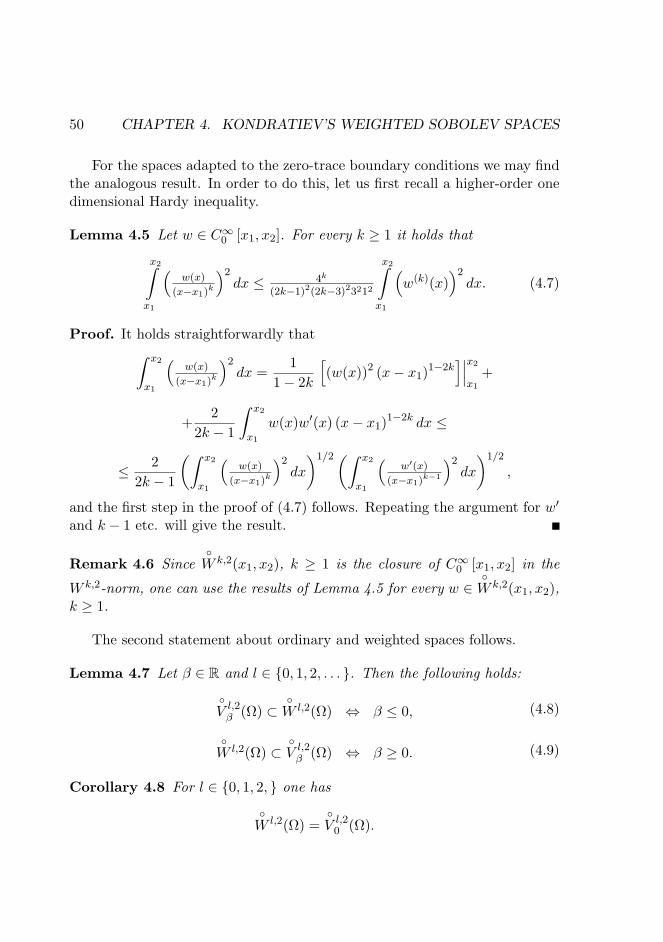
For the spaces adapted to the zero-trace boundary conditions we may findthe analogous result. In order to do this, let us first recall a higher-order onedimensional Hardy inequality.
Lemma 4.5 Let w ∈ C∞0 [x1, x2]. For every k ≥ 1 it holds that
x2∫x1
(w(x)
(x−x1)k
)2dx ≤ 4k
(2k−1)2(2k−3)23212
x2∫x1
(w(k)(x)
)2dx. (4.7)
Proof. It holds straightforwardly that∫ x2
x1
(w(x)
(x−x1)k
)2dx =
11− 2k
[(w(x))2 (x− x1)
1−2k]∣∣∣x2
x1
+
+2
2k − 1
∫ x2
x1
w(x)w′(x) (x− x1)1−2k dx ≤
≤ 22k − 1
(∫ x2
x1
(w(x)
(x−x1)k
)2dx
)1/2(∫ x2
x1
(w′(x)
(x−x1)k−1
)2dx
)1/2
,
and the first step in the proof of (4.7) follows. Repeating the argument for w′
and k − 1 etc. will give the result.
Remark 4.6 SinceW k,2(x1, x2), k ≥ 1 is the closure of C∞
0 [x1, x2] in the
W k,2-norm, one can use the results of Lemma 4.5 for every w ∈W k,2(x1, x2),
k ≥ 1.
The second statement about ordinary and weighted spaces follows.
Lemma 4.7 Let β ∈ R and l ∈ 0, 1, 2, . . . . Then the following holds:
V l,2β (Ω) ⊂
W l,2(Ω) ⇔ β ≤ 0, (4.8)
W l,2(Ω) ⊂
V l,2β (Ω) ⇔ β ≥ 0. (4.9)
Corollary 4.8 For l ∈ 0, 1, 2, one has
W l,2(Ω) =
V l,2
0 (Ω).
4.1. COMPARING (WEIGHTED) SOBOLEV SPACES: IMBEDDINGS 51
Proof of Lemma 4.7. Let Ω be as in Condition 1.2 with α ∈[0, 1
2π)
andω ∈ (0, 2π). Let us set θ = α+ 1
2ω. We also use the fact that for our domainthere exists c > 0 such that
r > cρ (x, y)
where ρ denotes the distance from a point (x, y) on the lines
` : y = tan (θ)x+ τ,
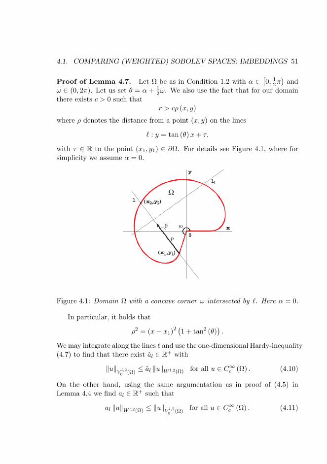
with τ ∈ R to the point (x1, y1) ∈ ∂Ω. For details see Figure 4.1, where forsimplicity we assume α = 0.
0
y
x
Ω)2y,2(x
)1y,1(x
ωθ
ρ
1l
l
Figure 4.1: Domain Ω with a concave corner ω intersected by `. Here α = 0.
In particular, it holds that
ρ2 = (x− x1)2 (1 + tan2 (θ)
).
We may integrate along the lines ` and use the one-dimensional Hardy-inequality(4.7) to find that there exist al ∈ R+ with
‖u‖V l,20 (Ω)
≤ al ‖u‖W l,2(Ω) for all u ∈ C∞c (Ω) . (4.10)
On the other hand, using the same argumentation as in proof of (4.5) inLemma 4.4 we find al ∈ R+ such that
al ‖u‖W l,2(Ω) ≤ ‖u‖V l,20 (Ω)
for all u ∈ C∞c (Ω) . (4.11)
52 CHAPTER 4. KONDRATIEV’S WEIGHTED SOBOLEV SPACES
Inequalities (4.10), (4.11) yield
W l,2(Ω) =
V l,2
0 (Ω).
Due to imbeddingV l,2β1
(Ω) ⊂V l,2
0 (Ω) ⊂V l,2β2
(Ω) when β1 ≤ 0 ≤ β2 one obtainsthe result in (4.8) and (4.9).
Chapter 5
Regularity results
In this Chapter we will give the regularity result to our clamped-grid problem(1.4):
uxxxx + uyyyy = f in Ω,
u = 0 on ∂Ω,∂∂nu = 0 on ∂Ω\0.
in the domain Ω defined as in Condition 1.2 (we sketch Ω in Figure below).In order to do this we refer to the key theorem of the Kondratiev theory
(see e.g. [19, Theorem 6.4.1]). We will also use the information from Chapter3 on the power type solutions to the homogeneous problem (3.1) in the coneK(α,ω).
5.1 General regularity statement
The Kondratiev theorem adapted to our problem (1.4) reads as:
Theorem 5.1 (Kondratiev) Let u ∈ V l1,2β1
(Ω) with l1 ∈ N, β1 ∈ R be asolution of the elliptic boundary value problem (1.4).
Suppose that f ∈ V l2,2β2
(Ω), where l2 ∈ N, β2 ∈ R and such that
l1 − β1 < l2 − β2 + 4.
If no eigenvalue λj of problem (3.4) lies on the lines
Re(λ) = l1 − β1 − 2, Re(λ) = l2 − β2 + 2,
53
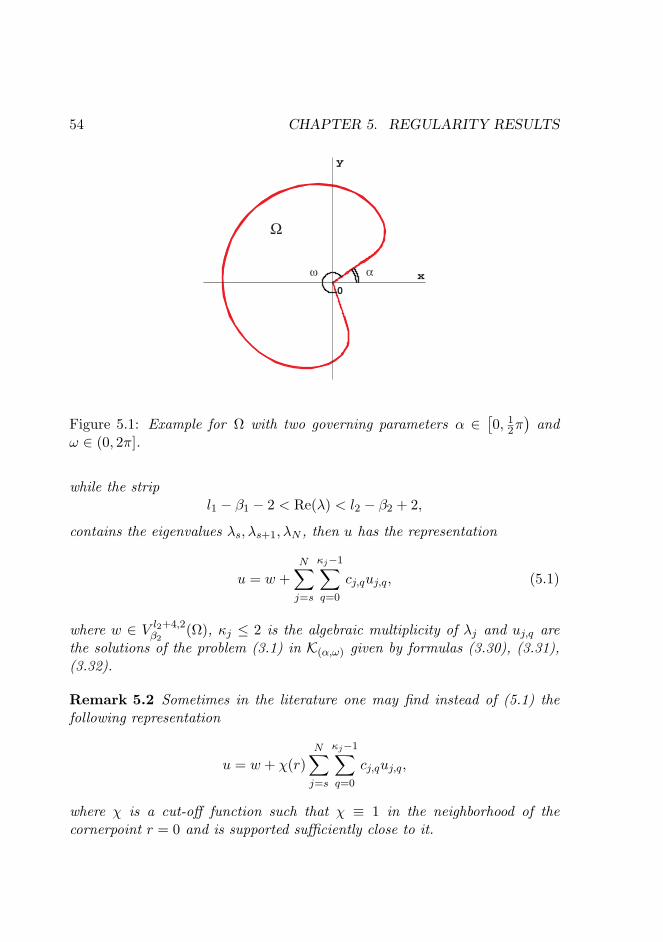
54 CHAPTER 5. REGULARITY RESULTS
0
y
x
Ω
ω α
Figure 5.1: Example for Ω with two governing parameters α ∈[0, 1
2π)
andω ∈ (0, 2π].
while the stripl1 − β1 − 2 < Re(λ) < l2 − β2 + 2,
contains the eigenvalues λs, λs+1, λN , then u has the representation
u = w +N∑j=s
κj−1∑q=0
cj,quj,q, (5.1)
where w ∈ V l2+4,2β2
(Ω), κj ≤ 2 is the algebraic multiplicity of λj and uj,q arethe solutions of the problem (3.1) in K(α,ω) given by formulas (3.30), (3.31),(3.32).
Remark 5.2 Sometimes in the literature one may find instead of (5.1) thefollowing representation
u = w + χ(r)N∑j=s
κj−1∑q=0
cj,quj,q,
where χ is a cut-off function such that χ ≡ 1 in the neighborhood of thecornerpoint r = 0 and is supported sufficiently close to it.
5.1. GENERAL REGULARITY STATEMENT 55
The statement above is too general. We specify it in the following way.
Recall that by Theorem 2.12 there exists a unique weak solution u ∈W 2,2(Ω)
of (1.4) with f ∈ L2(Ω). Since L2(Ω) = V 0,20 (Ω) and by Corollary 4.8 one
hasW 2,2(Ω) =
V 2,2
0 (Ω) ⊂ V 2,20 (Ω), we conclude that for f ∈ V 0,2
0 (Ω) wehave u ∈ V 2,2
0 (Ω). Then assuming more regularity for f ∈ V 0,20 (Ω) we apply
Theorem 5.1 to obtain:
Theorem 5.3 (Weighted space) Let f ∈ L2(Ω) and let u ∈W 2,2(Ω) be a
weak solution to (1.4).Suppose that f ∈ V k,2
β (Ω), where k ≥ 0, β ≤ k, and that no eigenvalue λjof problem (3.4) lies on the lines
Re(λ) = 0, Re(λ) = k − β + 2,
while the strip0 < Re(λ) < k − β + 2,
contains the eigenvalues λ1, λ2, λN . Then u has the representation
u = w +N∑j=1
κj−1∑q=0
cj,quj,q, (5.2)
where w ∈ V k+4,2β (Ω), κj ≤ 2 is the algebraic multiplicity of λj and uj,q are
the solutions of the problem (3.1) in K(α,ω) given by formulas (3.30), (3.31),(3.32).
The previous theorem gives the optimal regularity in the sense of Kon-dratiev’s spaces. Due to Lemmas 4.4 and 4.7 we are able to formulate theregularity statement in terms of commonly used Sobolev spaces, namely, when
f ∈
W k,2(Ω), k ≥ 1,
W k,2(Ω), k ≥ 0.
The result is as follows (for the convenience we arranged it as a table):
56 CHAPTER 5. REGULARITY RESULTS
Theorem 5.4 (Sobolev space) Let f ∈ L2(Ω) and let u ∈W 2,2(Ω) be a
weak solution to (1.4).
Suppose also that f ∈W k,2(Ω), k ≥ 1 W k,2(Ω), k ≥ 0
and that no eigenvalueλj of the problem
(3.4) lies on the lines,
Re(λ) = 0,
Re(λ) = k + 2
Re(λ) = 0,Re(λ) = 2
while the strip 0 < Re(λ) < k + 2 0 < Re(λ) < 2
contains the eigenvalues λ1, λ2, ..., λN .
Then u has therepresentation
u = w +∑N
j=1
∑κj−1q=0 cj,quj,q,
where w ∈ W k+4,2(Ω) W k+4,2(Ω, |x|2k dµ)
κj ≤ 2 is the algebraic multiplicity of λj and uj,q are the solutions of theproblem (3.1) in K(α,ω) given by formulas (3.30), (3.31), (3.32).
Remark 5.5 Away from the corner also these results are optimal. Of coursethe optimal regularity near a corner can not be stated using just the standardSobolev spaces W `,2(Ω).
Proof. For the first column one uses the imbeddingsW k,2(Ω) ⊂ V k,2
0 (Ω) and V k+4,20 (Ω) ⊂W k+4,2(Ω),
and for the second
W k,2(Ω) ⊂ V k,2k (Ω) and V k+4,2
k (Ω) ⊂W k+4,2(Ω, |x|2k dµ).
In Theorems 5.3 and 5.4 the function w is sometimes called in the lit-erature a regular part of the solution u ∈
W 2,2(Ω), as it preserves the full
regularity in a classical sense: f ∈ W k,2(Ω) ⇒ w ∈ W k+4,2(Ω). The double
sum∑N
j=1
∑κj−1q=0 cj,quj,q in the asymptotic representation for u ∈
W 2,2(Ω) is
then a so-called singular part. From formulas (3.30), (3.31), (3.32) we knowthat the first term of the sum, depending on the algebraic multiplicity of λ1,reads as
rλ1+1Φ1,0 (θ) or rλ1+1 (Φ1,1(θ) + log(r)Φ1,0(θ)) . (5.3)

5.2. REGULARITY FOR THE SINGULAR PART OF U 57
Here, λ1 ∈ C is the first eigenvalue of (3.4) such that Re(λ1) > 0 andΦ1,0(θ),Φ1,1(θ) ∈ C∞ [α, α+ ω], α ∈
[0, 1
2π), 0 < ω < 2π. Hence, in or-
der to complete our regularity analysis we will describe the regularity in Ω ofthe power type terms (5.3).
5.2 Regularity for the singular part of u
We start from the following lemma
Lemma 5.6 Let Ψ(θ) ∈ C∞ [α, α+ ω] be nontrivial and α ∈[0, 1
2π), 0 <
ω < 2π. Let also λ ∈ C\Z with Re(λ) > 0. Suppose that k ∈ 0, 1, 2, 3, . . . .Then the following are equivalent:
1. rλ+1Ψ(θ) ∈W k,2(Ω),
2. rλ+1 log(r)Ψ (θ) ∈W k,2(Ω),
3. Re(λ) + 1 > k − 1.
Proof. If λ is not an integer, one finds for R > 0 that rλ+1Ψ(θ) ∈ W k,2(Ω)means
R∫0
(rRe(λ)+1−k
)2rdr <∞.
This holds true when 2 (Re (λ) + 1− k) + 1 > −1 yielding the third item.Inclusion of a term with log(r) will not alter the regularity, so the same resultholds.
Remark 5.7 In order to restrict the already heavy technical aspects we havenot considered (weighted) Sobolev spaces with non-integer coefficients k andHolder spaces. A similar result will hold for k is non-integer. ConcerningHolder spaces:
rλ+1Ψ(θ) ∈ Ck,γ(Ω) for Re(λ) + 1 ≥ k + γ with k ∈ N, γ ∈ [0, 1) .
For the second function it holds that
rλ+1 log(r)Ψ (θ) ∈ Ck,γ(Ω) for Re(λ) + 1 > k + γ with k ∈ N, γ ∈ [0, 1) .
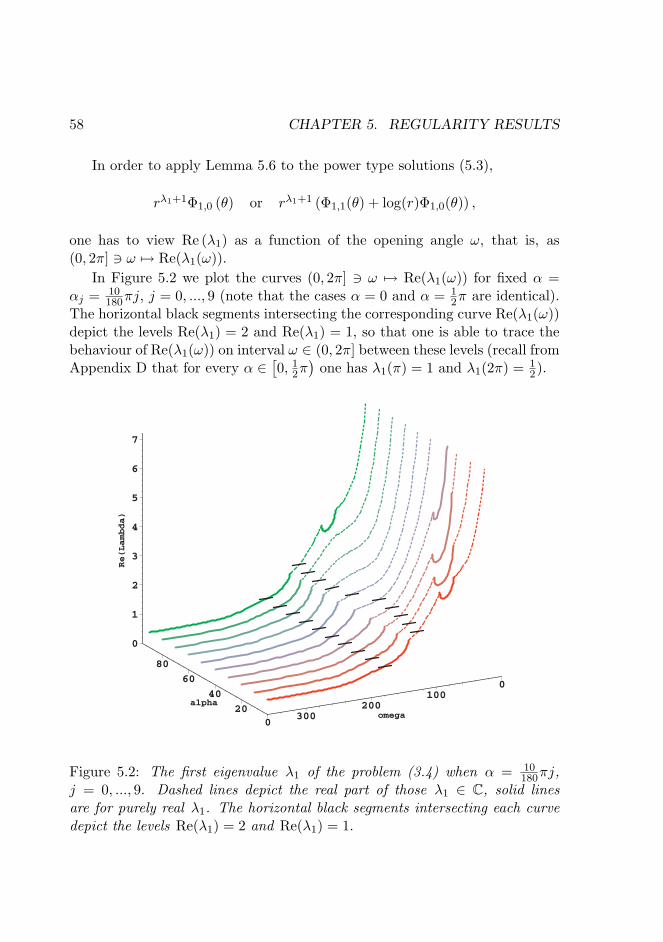
58 CHAPTER 5. REGULARITY RESULTS
In order to apply Lemma 5.6 to the power type solutions (5.3),
rλ1+1Φ1,0 (θ) or rλ1+1 (Φ1,1(θ) + log(r)Φ1,0(θ)) ,
one has to view Re (λ1) as a function of the opening angle ω, that is, as(0, 2π] 3 ω 7→ Re(λ1(ω)).
In Figure 5.2 we plot the curves (0, 2π] 3 ω 7→ Re(λ1(ω)) for fixed α =αj = 10
180πj, j = 0, ..., 9 (note that the cases α = 0 and α = 12π are identical).
The horizontal black segments intersecting the corresponding curve Re(λ1(ω))depict the levels Re(λ1) = 2 and Re(λ1) = 1, so that one is able to trace thebehaviour of Re(λ1(ω)) on interval ω ∈ (0, 2π] between these levels (recall fromAppendix D that for every α ∈
[0, 1
2π)
one has λ1(π) = 1 and λ1(2π) = 12).
020
40
60
80
alpha
0100
200300 omega
0
1
2
3
4
5
6
7
Re(Lambda)
Figure 5.2: The first eigenvalue λ1 of the problem (3.4) when α = 10180πj,
j = 0, ..., 9. Dashed lines depict the real part of those λ1 ∈ C, solid linesare for purely real λ1. The horizontal black segments intersecting each curvedepict the levels Re(λ1) = 2 and Re(λ1) = 1.
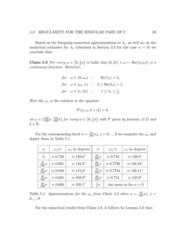
5.2. REGULARITY FOR THE SINGULAR PART OF U 59
Based on the foregoing numerical approximations to λ1, as well as, on theanalytical estimates for λ1 (obtained in Section 3.3 for the case α = 0) weconclude that:
Claim 5.8 For every α ∈[0, 1
2π)
it holds that (0, 2π] 3 ω 7→ Re(λ1(ω)) is acontinuous function. Moreover,
for ω ∈ (0, ω?) : Re(λ1) > 2,
for ω ∈ [ω?, π) : 2 ≥ Re(λ1) > 1,
for ω ∈ [π, 2π] : 1 ≥ λ1 ≥ 12 .
Here the ω? is the solution to the equation
P (α, ω, 2 + iξ) = 0,
on ω ∈(
100180π,
150180π
)for every α ∈
[0, 1
2π)
with P given by formula (3.7) andξ ∈ R.
For the corresponding fixed α = 10180πj, j = 0, ..., 9 we compute the ω? and
depict them in Table 5.1.
α ω?/π ω? in degrees α ω?/π ω? in degrees
0 ≈ 0.720 ≈ 129.6 50180π ≈ 0.716 ≈ 129.0
10180π ≈ 0.681 ≈ 122.6 60
180π ≈ 0.7786 ≈ 140.16
20180π ≈ 0.640 ≈ 115.3 70
180π ≈ 0.7784 ≈ 140.11
30180π ≈ 0.605 ≈ 108.9 80
180π ≈ 0.754 ≈ 135.8
40180π ≈ 0.600 ≈ 108.1 1
2π the same as for α = 0
Table 5.1: Approximations for the ω? from Claim 5.8 when α = 10180πj, j =
0, ..., 9.
For the numerical results from Claim 5.8, it follows by Lemma 5.6 that:

60 CHAPTER 5. REGULARITY RESULTS
Claim 5.9 For every α ∈[0, 1
2π)
it holds that power type term in (5.3) belongsto
W 4,2(Ω) when ω ∈ (0, ω?),
W 3,2(Ω) when ω ∈ [ω?, π),
C∞ (Ω) when ω = π,
W 2,2(Ω) when ω ∈ (π, 2π].
Remark 5.10 When the opening angle ω = π we know from Appendix D thatevery term uj,q of the singular part
∑Nj=1
∑κj−1q=0 cj,quj,q is a polynomial in x, y
of order λj + 1. That is, for every λj, j ∈ N+ we have
rλj+1Φj (θ) = Pλj+1(x, y) ∈ C∞ (Ω) . (5.4)
For non-polynomials the result in Lemma 5.6 even holds for λ ∈ N.
5.3 Corollary
For the numerical results from Claim 5.9, it holds by Theorem 5.4 that:
Corollary 5.11 Let u ∈W 2,2(Ω) be a weak solution of problem (1.4) with
f ∈ L2(Ω). Then
for ω ∈ (0, ω?) : u ∈W 4,2(Ω),
for ω ∈ (ω?, π) : u ∈W 3,2(Ω),
for ω = π : u ∈W 4,2(Ω),
for ω ∈ (π, 2π] : u ∈W 2,2(Ω).
Here ω? is as in Claim 5.8.
Remark 5.12 For opening angle ω = ω? we have Re (λ1) = 2 and henceTheorem 5.4 does not apply. Nevertheless, assuming f ∈ L2(Ω) to be more
regular, e.g. in V 1,20 (Ω) or
W 1,2(Ω), we may show that
for ω = ω? : u ∈W 3,2(Ω).
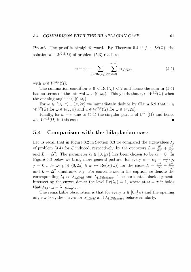
5.4. COMPARISON WITH THE BILAPLACIAN CASE 61
Proof. The proof is straightforward. By Theorem 5.4 if f ∈ L2(Ω), the
solution u ∈W 2,2(Ω) of problem (5.3) reads as
u = w +∑
0<Re(λj)<2
κj−1∑q=0
cj,quj,q, (5.5)
with w ∈W 4,2(Ω).The summation condition is 0 < Re (λj) < 2 and hence the sum in (5.5)
has no terms on the interval ω ∈ (0, ω?). This yields that u ∈ W 4,2(Ω) whenthe opening angle ω ∈ (0, ω?).
For ω ∈ (ω?, π) ∪ (π, 2π] we immediately deduce by Claim 5.9 that u ∈W 3,2(Ω) for ω ∈ (ω?, π) and u ∈W 2,2(Ω) for ω ∈ (π, 2π].
Finally, for ω = π due to (5.4) the singular part is of C∞ (Ω) and henceu ∈W 4,2(Ω) in this case.
5.4 Comparison with the bilaplacian case
Let us recall that in Figure 3.2 in Section 3.3 we compared the eigenvalues λjof problem (3.4) for L induced, respectively, by the operators L = ∂4
∂x4 + ∂4
∂y4
and L = ∆2. The parameter α ∈[0, 1
2π)
has been chosen to be α = 0. InFigure 5.3 below we bring more general picture: for every α = αj = 10
180πj,j = 0, ..., 9 we plot (0, 2π] 3 ω 7→ Re(λ1(ω)) for the cases L = ∂4
∂x4 + ∂4
∂y4
and L = ∆2 simultaneously. For convenience, in the caption we denote thecorresponding λ1 as λ1,Grid and λ1,Bilaplace. The horizontal black segmentsintersecting the curves depict the level Re(λ1) = 1, where at ω = π it holdsthat λ1,Grid = λ1,Bilaplace.
The remarkable observation is that for every α ∈[0, 1
2π)
and the openingangle ω > π, the curves for λ1,Grid and λ1,Bilaplace behave similarly.
62 CHAPTER 5. REGULARITY RESULTS
020
40
60
80
alpha
0100
200300 omega
0
1
2
3
4
5
6
7
Re(Lambda)
Figure 5.3: The first eigenvalue λ1of the problem (3.4) when α = 10180πj, j =
0, ..., 9. For L in (3.4) induced, respectively, by the operators L = ∂4
∂x4 + ∂4
∂y4and
L = ∆2, we have λ1,Grid (colored) and λ1,Bilaplace (in blue). The horizontalblack segments depict the level Re(λ1) = 1, where at ω = π it holds that thevalues λ1,Grid and λ1,Bilaplace are identical.
Chapter 6
System approach to theclamped grid problem
A solution of a fourth order elliptic boundary value problem can be obtainedeither directly or by considering a system of second order equations. Thesystem approach is usually favorized for numerical methods since one mayuse piecewise linear C0,1 finite elements, instead of piecewise quadratic C1,1
elements needed for the direct approach. Thus, in [13] the authors compareboth approaches for the clamped plate problem and proved that for planardomains with reentrant (i.e. concave) corners the system approach failed toproduce the correct solution. In this chapter we will study the similar questionfor our clamped grid problem. The material of Chapter 5 will be of use in thisstudy.
6.1 Outline and settings
Let Ω ⊂ R2 be open and bounded. In Chapter 2 we show that for any f ∈L2(Ω) the clamped grid problem
uxxxx + uyyyy = f in Ω,
u = ∂∂nu = 0 on ∂Ω,
(6.1)
63

64CHAPTER 6. SYSTEM APPROACH TO THE CLAMPED GRID PROBLEM
has a unique weak solutionW 2,2(Ω). This weak solution is a minimizer of the
energy functional
E [u] =∫Ω
(12
(u2xx + u2
yy
)− fu
)dxdy over
W 2,2(Ω),
and a solution to the weak Euler-Lagrange equation∫Ω
(uxxϕxx + uyyϕyy − fϕ) dxdy = 0 for all ϕ ∈W 2,2(Ω). (6.2)
Alternatively one may consider a system of second order equations. Indeed,due to the factorization
∂4
∂x4 + ∂4
∂y4=(−∆−
√2 ∂2
∂x∂y
)(−∆ +
√2 ∂2
∂x∂y
),
problem (6.1) will be split into:−∆v −
√2vxy = f in Ω,
−∆u+√
2uxy = v in Ω,
u = ∂∂nu = 0 on ∂Ω.
(6.3)
A weak solution for the system is a pair (v, u) ∈W 1,2(Ω)×W 1,2(Ω) such that∫
Ω
[(∂v∂x +
√2
2∂v∂y
)∂ψ∂x +
(∂v∂y +
√2
2∂v∂x
)∂ψ∂y+
+(∂u∂x −
√2
2∂u∂y
)∂φ∂x +
(∂u∂y −
√2
2∂u∂x
)∂φ∂y − fψ − vφ
]dxdy = 0,
for all (φ, ψ) ∈W 1,2(Ω)×W 1,2(Ω). (6.4)
Remark 6.1 Assuming for a moment (v, u) to be more regular, an integrationby parts in (6.4) leads to
0 =∫Ω
(−∆v −
√2 ∂2v∂x∂y − f
)ψdxdy +
∫Ω
(−∆u+
√2 ∂2u∂x∂y − v
)φdxdy+

6.1. OUTLINE AND SETTINGS 65
+∫∂Ω
(n1
(∂v∂x +
√2
2∂v∂y
)+ n2
(∂v∂y +
√2
2∂v∂x
))ψdS+
+∫∂Ω
(n1
(∂u∂x −
√2
2∂u∂y
)+ n2
(∂u∂y −
√2
2∂u∂x
))φdS,
where n = (n1, n2) is the unit outward normal vector on ∂Ω. The first two inte-grals formally results in the equations −∆v−
√2 ∂2v∂x∂y = f , −∆u+
√2 ∂2u∂x∂y = v
in Ω. The first boundary integral vanishes due to ψ = 0 on ∂Ω. The lat-ter boundary integral being equal to zero results in second boundary condition∂u∂n = 0 on ∂Ω. Indeed, in terms of the normal and tangential derivatives onehas ∂u
∂x = n1∂u∂n − n2
∂u∂τ and ∂u
∂y = n2∂u∂n + n1
∂u∂τ . Moreover, u = 0 on ∂Ω and
hence ∂u∂τ = 0 on ∂Ω. As a result we deduce that
0 =∫∂Ω
(n1
(∂u∂x −
√2
2∂u∂y
)+ n2
(∂u∂y −
√2
2∂u∂x
))φdS =
=∫∂Ω
(1−
√2n1n2
)∂u∂nφdS. (6.5)
Since the normal (n1, n2) = (cos(γ), sin(γ)) one finds that n1n2 = 12 sin(2γ) ∈[
−12 ,
12
]and hence that 1 −
√2n1n2 ≥ 1 −
√2
2 > 0. The factor in (6.5) ispositive and hence we obtain ∂u
∂n = 0 on ∂Ω as a second boundary condition.
The reason why we want to use the system approach (6.3) in order to solvethe original fourth order problem (6.1) is that such an approach has an advan-tage from the computational point of view. Indeed, in order to approximate(v, u) to (6.3) one may use piecewise linear C0,1 finite elements, which are im-plemented in a large number of standard programming libraries. The solutionu to (6.1) has to be approximated by piecewise quadratic C1,1 elements in or-der to avoid δ-type distributions behavior over the edges of adjacent elements.C. Davini in [8] follows an alternative approach by introducing a numericalway of treating distributions over mesh-sides which allowed him to stay withthe piecewise linear C0,1 elements.
The solutions u of both problems, however, may not coincide and whetherit happens or not depends on the properties of the domain Ω. In particular,it holds that u of (6.1) and u in the solution (v, u) of (6.3) are identical when

66CHAPTER 6. SYSTEM APPROACH TO THE CLAMPED GRID PROBLEM
Ω is smooth or has a convex corner. For the case when a reentrant (concave)corner is presented in Ω, this does not hold true. Below we will give a detailedexplanation and proof to these results.
6.2 System approach
Let us setH = W 1,2(Ω)×
W 1,2(Ω).
First we have to find out the existence of a solution (v, u) ∈ H to the in-tegral equation (6.4). Unfortunately, one is not able to recover a functionalH(v, u) such that ∂H(v, u;φ, ψ) would equal to the left-hand side of (6.4),so we can not talk about (v, u) of (6.4) in terms of a stationary point of acertain functional. Instead, we will show that if we assume some additional
regularity of the corresponding solutions, the solution u ∈W 2,2(Ω) of (6.2)
and a solution (v, u) ∈ H of (6.4) will coincide. Then there will be a one toone correspondence implying that (v, u) exists and is unique.
Proposition 6.2 Let Ω ⊂ R2 be open and bounded and let f ∈ L2(Ω).
1. If (v, u) ∈ H is a solution of (6.4) and u ∈ W 2,2(Ω) then u satisfies theequation (6.2).
2. If u ∈W 2,2(Ω) satisfies (6.2) and −∆u +
√2uxy ∈ W 1,2(Ω), then(
−∆u+√
2uxy, u)
is a solution of (6.4).
Proof.
1. Let (v, u) ∈ H be a solution of of (6.4). Then we have∫Ω
[(∂v∂x +
√2
2∂v∂y
)∂ψ∂x +
(∂v∂y +
√2
2∂v∂x
)∂ψ∂y − fψ
]dxdy = 0,
for all ψ ∈W 1,2(Ω), (6.6)∫
Ω
[(∂u∂x −
√2
2∂u∂y
)∂φ∂x +
(∂u∂y −
√2
2∂u∂x
)∂φ∂y − vφ
]dxdy = 0,
for all φ ∈W 1,2(Ω). (6.7)

6.2. SYSTEM APPROACH 67
If u ∈W 2,2(Ω), the for all φ ∈W 1,2(Ω) we derive from (6.7) that
0 =∫Ω
(−∆u+
√2 ∂2u∂x∂y − v
)φdxdy+
+∫∂Ω
(n1
(∂u∂x −
√2
2∂u∂y
)+ n2
(∂u∂y −
√2
2∂u∂x
))φdS,
which implies −∆u +√
2 ∂2u∂x∂y = v in Ω and ∂u
∂n = 0 on ∂Ω in a weaksense (for the latter condition see formula (6.5) in Remark 6.1). Hence,
u ∈W 2,2(Ω). Moreover, by density,∫
Ω
(−∆u+
√2 ∂2u∂x∂y − v
)φdxdy = 0, for all φ ∈ L2(Ω).
Taking ψ ∈W 2,2(Ω) and using φ = −∆ψ −
√2 ∂2ψ∂x∂y we find with (6.6)
that
0 =∫Ω
(−∆u+
√2 ∂2u∂x∂y − v
)(−∆ψ −
√2 ∂2ψ∂x∂y
)dxdy =
=∫Ω
(uxxψxx + uyyψyy − fψ) dxdy.
2. Let us define the left-hand side of equation (6.4) as A(v, u;φ, ψ). Here
we will prove that if (6.2) holds true and u ∈W 2,2(Ω), −∆u+
√2uxy ∈
W 1,2(Ω) then
A(−∆u+√
2uxy, u;φ, ψ) = 0, for all (φ, ψ) ∈ H.
Indeed, for u ∈W 2,2(Ω) and −∆u+
√2uxy ∈W 1,2(Ω) it holds that
0 =∫Ω
(uxxψxx + uyyψyy − fψ) dxdy =
=∫Ω
[(∂∂x
(−∆u+
√2uxy
)+
√2
2∂∂y
(−∆u+
√2uxy
))∂ψ∂x +

68CHAPTER 6. SYSTEM APPROACH TO THE CLAMPED GRID PROBLEM
+(∂∂y
(−∆u+
√2uxy
)+
√2
2∂∂x
(−∆u+
√2uxy
))∂ψ∂y − fψ
]dxdy,
for all ψ ∈W 2,2(Ω).
SinceW 2,2(Ω) is dense in
W 1,2(Ω) one has for the above equation that
0 =∫Ω
[(∂∂x
(−∆u+
√2uxy
)+
√2
2∂∂y
(−∆u+
√2uxy
))∂ψ∂x +
+(∂∂y
(−∆u+
√2uxy
)+
√2
2∂∂x
(−∆u+
√2uxy
))∂ψ∂y − fψ
]dxdy,
for all ψ ∈W 1,2(Ω).
Then it follows that
A(−∆u+√
2uxy, u;φ, ψ) =
=∫Ω
[(∂∂x
(−∆u+
√2uxy
)+
√2
2∂∂y
(−∆u+
√2uxy
))∂ψ∂x +
+(∂∂y
(−∆u+
√2uxy
)+
√2
2∂∂x
(−∆u+
√2uxy
))∂ψ∂y+
+(∂u∂x −
√2
2∂u∂y
)∂φ∂x +
(∂u∂y −
√2
2∂u∂x
)∂φ∂y
−fψ −(−∆u+
√2uxy
)φ]dxdy =
=∫Ω
[(∂u∂x −
√2
2∂u∂y
)∂φ∂x +
(∂u∂y −
√2
2∂u∂x
)∂φ∂y −
(−∆u+
√2uxy
)φ]dxdy =
=∫∂Ω
(1−
√2n1n2
)∂u∂nφdS = 0,
holds for all (φ, ψ) ∈ H.

6.3. COMPARING MINIMIZING AND SYSTEM APPROACH 69
6.3 Comparing minimizing and system approach
Let us recall that the two different types of weak solution we obtain for problem(6.1).
• Minimizer of the energy functional E [u] =∫Ω
(12
(u2xx + u2
yy
)− fu
)dxdy
overW 2,2(Ω) yields a solution u ∈
W 2,2(Ω).
• A solution of equation (6.4) gives a solution u ∈W 1,2(Ω) with −∆u +√
2uxy ∈W 1,2(Ω) and∫Ω
(−∆u+
√2 ∂2u∂x∂y
)φdxdy =
=∫Ω
((∂u∂x −
√2
2∂u∂y
)∂φ∂x +
(∂u∂y −
√2
2∂u∂x
)∂φ∂y
)dxdy.
The last equation replaces the zero normal derivative of u.
Here we will compare these solutions by specifying the properties of thedomain Ω in which problem (6.1) is posed. To be more precise, let Ω be definedas in Condition 1.2 (the sketch of Ω is depicted in Figure 6.1 below).
We claim the following.
Lemma 6.3 The minimizer u of the clamped grid problem (6.1) satisfies−∆u+
√2uxy ∈W 1,2(Ω) if and only if ω ≤ π.
Proof. The result follows by Corollary 5.11 from Chapter 5.
Corollary 6.4 Assume that the domain Ω as in above. Then equation (6.4)possesses a solution in H.
Proof. It is enough to apply Lemma 6.3 with Proposition 6.2 to obtain thatthe unique minimizer of E [u] =
∫Ω
(12
(u2xx + u2
yy
)− fu
)dxdy is a solution of
(6.4).Now we proceed with the comparison of the two solutions in the case when
ω > π, i.e. when Ω has a concave (reentrant) corner. We will see that thesystem approach will, in general, not agree with the minimization problem.
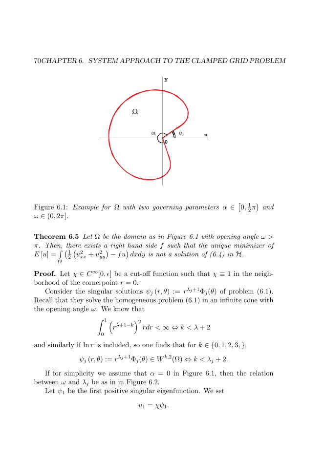
70CHAPTER 6. SYSTEM APPROACH TO THE CLAMPED GRID PROBLEM
0
y
x
Ω
ω α
Figure 6.1: Example for Ω with two governing parameters α ∈[0, 1
2π)
andω ∈ (0, 2π].
Theorem 6.5 Let Ω be the domain as in Figure 6.1 with opening angle ω >π. Then, there exists a right hand side f such that the unique minimizer ofE [u] =
∫Ω
(12
(u2xx + u2
yy
)− fu
)dxdy is not a solution of (6.4) in H.
Proof. Let χ ∈ C∞[0, ε] be a cut-off function such that χ ≡ 1 in the neigh-borhood of the cornerpoint r = 0.
Consider the singular solutions ψj (r, θ) := rλj+1Φj(θ) of problem (6.1).Recall that they solve the homogeneous problem (6.1) in an infinite cone withthe opening angle ω. We know that∫ 1
0
(rλ+1−k
)2rdr <∞⇔ k < λ+ 2
and similarly if ln r is included, so one finds that for k ∈ 0, 1, 2, 3, ,
ψj (r, θ) := rλj+1Φj(θ) ∈W k,2(Ω) ⇔ k < λj + 2.
If for simplicity we assume that α = 0 in Figure 6.1, then the relationbetween ω and λj be as in in Figure 6.2.
Let ψ1 be the first positive singular eigenfunction. We set
u1 = χψ1.
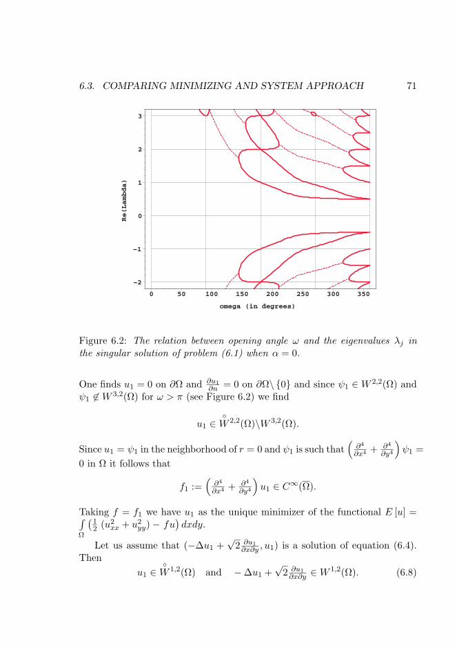
6.3. COMPARING MINIMIZING AND SYSTEM APPROACH 71
–2
–1
0
1
2
3Re(Lambda)
0 50 100 150 200 250 300 350
omega (in degrees)
Figure 6.2: The relation between opening angle ω and the eigenvalues λj inthe singular solution of problem (6.1) when α = 0.
One finds u1 = 0 on ∂Ω and ∂u1∂n = 0 on ∂Ω\ 0 and since ψ1 ∈W 2,2(Ω) and
ψ1 6∈W 3,2(Ω) for ω > π (see Figure 6.2) we find
u1 ∈W 2,2(Ω)\W 3,2(Ω).
Since u1 = ψ1 in the neighborhood of r = 0 and ψ1 is such that(∂4
∂x4 + ∂4
∂y4
)ψ1 =
0 in Ω it follows that
f1 :=(∂4
∂x4 + ∂4
∂y4
)u1 ∈ C∞(Ω).
Taking f = f1 we have u1 as the unique minimizer of the functional E [u] =∫Ω
(12 (u2
xx + u2yy)− fu
)dxdy.
Let us assume that (−∆u1 +√
2 ∂u1∂x∂y , u1) is a solution of equation (6.4).
Thenu1 ∈
W 1,2(Ω) and −∆u1 +
√2 ∂u1∂x∂y ∈W
1,2(Ω). (6.8)

72CHAPTER 6. SYSTEM APPROACH TO THE CLAMPED GRID PROBLEM
Applying Theorem 5.1 from Chapter 5 adapted to the spaceW 1,2(Ω), one
finds that the solution u1 ∈W 1,2(Ω) possesses the asymptotic representation
u1 = u1 + c−2ψ−2 + c−1ψ−1 + c1ψ1 + c2ψ2
(+ higher order terms
),
where u1 ∈W 4,2(Ω) and
ψ−2, ψ−1 ∈W 1,2(Ω)\W 2,2(Ω) and ψ1, ψ2 ∈W 2,2(Ω)\W 3,2(Ω).
The higher order terms lie in W 3,2(Ω). Moreover, since the functions ψi aresuch that (
−∆ +√
2 ∂∂x∂y
)ψi 6= 0,
one obtains (−∆ +
√2 ∂∂x∂y
)ψ−2,
(−∆ +
√2 ∂∂x∂y
)ψ−1 6∈ L2(Ω),
and (−∆ +
√2 ∂∂x∂y
)ψ1,(−∆ +
√2 ∂∂x∂y
)ψ2 6∈W 1,2(Ω),
and that they do not cancel each others singularity near 0. Hence, if −∆u1 +√2 ∂u1∂x∂y ∈ W
1,2(Ω), then by the second condition in (6.8) one is forced to set
c−2 = c−1 = c1 = c2 = 0. One finds u1 ∈W 3,2(Ω) ∩W 2,2(Ω), a contradiction.
Remark 6.6 The asymptotic analysis of the original fourth order problem andthe system approach produces the same boundary value problems and imposesnaturally the same boundary conditions on the angular eigenfunctions. Thusproduces the exact same singular eigenfunctions ψj.
Remark 6.7 Following the argumentation of the previous theorem, one seesthat when ω ≤ π, the stationary point is indeed in W 2,2(Ω). Thus, Proposition6.2 implies that it is unique.
Appendix A
Algebraic transformation
The main result of this appendix is that for every fourth order elliptic operator
L =∂4
∂x4+ b1
∂4
∂x3∂y+ b2
∂4
∂x2∂y2+ b3
∂4
∂x∂y3+
∂4
∂y4, (A.1)
with bj ∈ R, j = 1, 2, 3 there exists precisely one a ∈ [1,+∞) such that L isalgebraically equivalent to the operator
La =∂4
∂x4+ 2a
∂4
∂x2∂y2+
∂4
∂y4. (A.2)
This means that one may always find an appropriate linear coordinate trans-formation such that due to this transformation L turns into La.
A.1 Ellipticity of operator La
Let x ∈ Rn. Recall (see e.g. [25, Chapter 2, Definition 1.1]) that
Definition A.1 The differential operator of order 2m,
A
(∂
∂x
)=
∑|γ|=2m
bγ
(∂
∂x
)γ, (A.3)
where bγ ∈ R, is said to be elliptic if its symbol satisfies
A(ξ) 6= 0 for all ξ ∈ Rn\0.
73
74 APPENDIX A. ALGEBRAIC TRANSFORMATION
From the ellipticity it follows that A(ξ) ≥ c |ξ|2m for all ξ ∈ Rn, where cis a positive constant independent of ξ. Moreover, by Proposition 1.1 in [25,Chapter 2, Definition 1.1] it follows that if A is elliptic then the equation
C 3 τ 7→ A(ξ + τη) = 0,
where ξ, η ∈ Rn are linearly independent vectors, does not have any real roots.Then the following holds.
Lemma A.2 The operator La = ∂4
∂x4 + 2a ∂4
∂x2∂y2+ ∂4
∂y4is elliptic iff a > −1.
Proof. For a = 0 it holds that
ξ41 + ξ42 = 12
(ξ21 + ξ22
)2 + 12
(ξ21 − ξ22
)2 ≥ 12 |ξ|
4 ,
for all ξ ∈ R2. Then for a > 0 we it is straightforwardly that
ξ41 + 2aξ21ξ22 + ξ42 ≥ ξ41 + ξ42 ≥ 1
2 |ξ|4 .
Let a < 0. We set b = −a (that is, b > 0) and by Cauchy’s inequalityobtain
ξ41 − 2bξ21ξ22 + ξ42 ≥ ξ41 + ξ42 − b
(ξ41 + ξ42
)= (1− b)
(ξ41 + ξ42
)≥ 1
2 (1− b) |ξ|4 .
Hence, 1 − b > 0 and as a result, 0 < b < 1. In terms of a this yields−1 < a < 0.
Let a ∈ (−1,+∞) in La. The corresponding characteristic equation
τ4 + 2aτ2 + 1 = 0,
has four solutions τ1, τ2, τ1, τ2, where
τ1 = −√
22(√
1− a− i√
1 + a),
τ2 =√
22(√
1− a+ i√
1 + a), when a ∈ (−1, 1],
and
τ1 = i
√a−
√a2 − 1,
τ2 = i
√a+
√a2 − 1, when a ∈ [1,+∞).

A.2. TRANSFORMING THE ROOTS 75
In Figure A.1 we depict the location of τ1, τ2, τ1, τ2 on the complex planein dependence on a. In particular, for a ∈ (−1, 1) the roots lie on the unitcircle (in red) and a ∈ (1,+∞), they lie on the imaginary axis (in blue). Thea = 1 corresponds to the intersection point of the circle and the imaginaryaxis.
a=0 a=0
a=0 a=0
a=–1 a=–1
a=1
a=1
Im
Re
–1<a<11<a
Figure A.1: Diagram showing two possibilities in the location of the roots τ ∈ Cof the characteristic equation τ4 + 2aτ2 + 1 = 0, a ∈ (−1,+∞).
A.2 Transforming the roots
Let us first prove the simple yet useful lemma.
Lemma A.3 Let bj ∈ R, j = 1, 2, 3 be such that p(τ) := τ4 + b1τ3 + b2τ
2 +b3τ
2 + 1 has complex roots which come pairwise.
There exists a Mobius mapping f(z) =α+ βz
γ + δz, with real coefficients and
αδ 6= βγ, such that p (f(τ)) = 0 will have purely imaginary roots. Moreover,these roots are pairwise symmetric with respect to 0.
76 APPENDIX A. ALGEBRAIC TRANSFORMATION
Proof. Under assumption that the equation p(τ) = 0 has four complex rootscoming pairwise, let us denoting them as τ1, τ2, τ1, τ2 and write down
p(τ) = (τ − τ1) (τ − τ2) (τ − τ1) (τ − τ2) .
It holds that |τ1|2 |τ2|2 = 1.
Let f(z) =α+ βz
γ + δzbe the mapping to apply. We obtain
p (f(τ)) = (f(τ)− τ1) (f(τ)− τ2) (f(τ)− τ1) (f(τ)− τ2) =
=(α+ βτ
γ + δτ− τ1
)(α+ βτ
γ + δτ− τ2
)(α+ βτ
γ + δτ− τ1
)(α+ βτ
γ + δτ− τ2
)=
= A
(τ − −α+ γτ1
β − δτ1
)(τ − −α+ γτ2
β − δτ2
)(τ − −α+ γτ1
β − δτ1
)(τ − −α+ γτ2
β − δτ2
)=
= A(τ − f inv(τ1)
) (τ − f inv(τ2)
) (τ − f inv(τ1)
) (τ − f inv(τ2)
),
where A = 1(γ+δτ)4
(β − δτ1) (β − δτ2) (β − δτ1) (β − δτ2) and f inv stands forthe mapping inverse to f . This inverse mapping is again a Mobius mapping:
indeed, for f(z) =α+ βz
γ + δz, the inverse reads as f inv(w) =
−α+ γw
β − δw.
In order to see that f inv turns the roots τ1, τ2, τ1, τ2 into purely imaginaryvalues we consider two cases.
Case 1: the roots τ1, τ2, τ1, τ2 lie one one line (see Figure A.2, top), thatis, Re(τ1) = Re(τ2) and we suppose that 0 < Im(τ1) < Im(τ2). Then in orderto make τ1, τ2, τ1, τ2 purely imaginary a shift suffices, that is,
f inv(w) = w − Re(τ1).
The coefficients in f inv and f will read as:
α = Re(τ1), β = 1, δ = 0, γ = 1. (A.4)
One sees that αδ = 0 and βγ = 1. Hence αδ 6= βγ.Case 2: the roots τ1, τ2, τ1, τ2 are not on line, i.e. Re(τ1) 6= Re(τ2) and we
suppose that Im(τ1) and Im(τ2) are positive. Then they lie on one circle Cwhich is symmetric with respect to the real axis (see Figure A.2, bottom).
Let χ1 and χ2 denote the intersection points of this circle C with the realaxis. Then we take
f inv(w) =w − χ1
w − χ2.
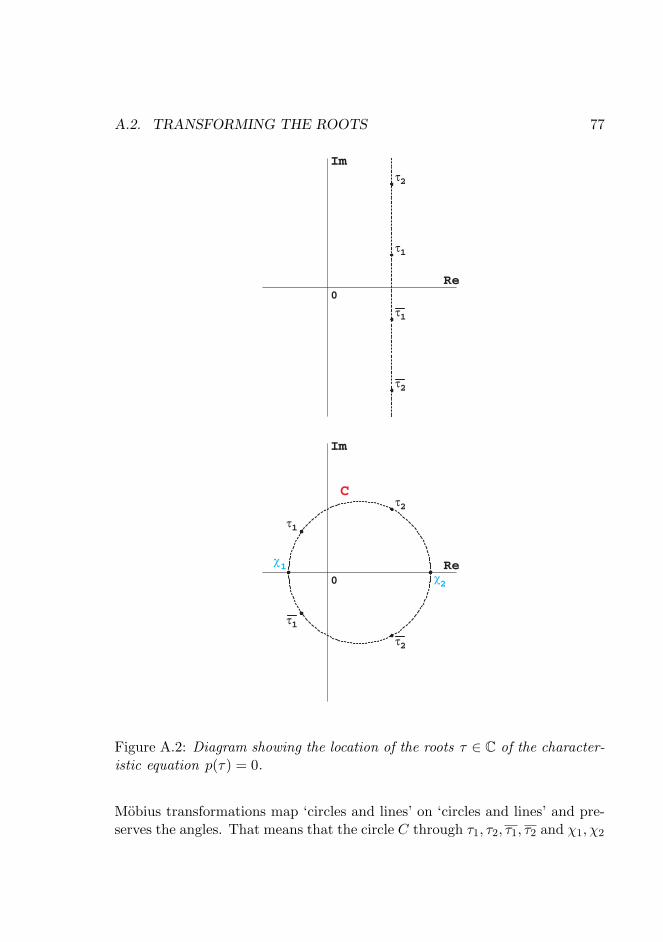
A.2. TRANSFORMING THE ROOTS 77
2τ
1τ
1τ
2τ
0
Im
Re
1χ
2χ
1τ
2τ
2τ
1τ
0
Im
Re
C
Figure A.2: Diagram showing the location of the roots τ ∈ C of the character-istic equation p(τ) = 0.
Mobius transformations map ‘circles and lines’ on ‘circles and lines’ and pre-serves the angles. That means that the circle C through τ1, τ2, τ1, τ2 and χ1, χ2
78 APPENDIX A. ALGEBRAIC TRANSFORMATION
will be again a circle or line. In fact, due to f inv(χ2) = ∞ we conclude thatmapped C is a line (let us denote it as `). The real axis is mapped on thereal axis and since the circle C intersects the real axis perpendicularly, theline ` will intersect the real line perpendicularly too. Since f inv(χ1) = 0, thisintersection is at 0. In other words, the image ` of the circle C is the imaginaryaxis.
The coefficients in f inv and f in this case are as follows as:
α = χ1, β = −χ2, δ = −1, γ = 1. (A.5)
One sees that αδ = −χ1 and βγ = −χ2. Hence αδ 6= βγ.Let us note that due to the symmetry of τ1, τ1 and τ2, τ2 with respect to
the real axis in both cases the transformation preserves this symmetry (seeFormula (A.7) for details).
For practical reasons it is useful to have the explicit formulas for f inv(w) =−α+ γw
β − δwto be applied to τj , j = 1, 2. In particular,
• When Re(τ1) = Re(τ2), one obtains directly that
f inv(τj) = iIm(τj), j = 1, 2. (A.6)
Here i =√−1.
• When Re(τ1) 6= Re(τ2), one finds for τj , j = 1, 2 that
f inv(τj) =τj − χ1
τj − χ2=
Re(τj) + iIm(τj)− χ1
Re(τj) + iIm(τj)− χ2=
=χ1χ2 − (χ1 + χ2) Re(τj) + |τj |2 + i (χ1 − χ2) Im(τj)
χ22 − 2χ2Re(τj) + |τj |2
.
We know that f inv(τj) is purely complex, meaning that
χ1χ2 − (χ1 + χ2) Re(τj) + |τj |2 = 0, j = 1, 2.
That is, as a result
f inv(τj) = i(χ1 − χ2) Im(τj)
χ22 − 2χ2Re(τj) + |τj |2
, j = 1, 2, (A.7)

A.2. TRANSFORMING THE ROOTS 79
where χ1,χ2 read as
χ1 =1
2 (Re(τ1)− Re(τ2))
(|τ1|2 − |τ2|2 ±
√D), (A.8)
χ2 =1
2 (Re(τ1)− Re(τ2))
(|τ1|2 − |τ2|2 ∓
√D), (A.9)
andD =
(|τ1|2 − |τ2|2
)2+ 4
(|τ1|2 Re2(τ2) + |τ2|2 Re2(τ1)
)+
−4Re(τ1)Re(τ2)(|τ1|2 + |τ2|2
).
Remark A.4 Note that the above D is always positive. Indeed, havingRe(τj) = |τj | cos(θj), j = 1, 2 and that |τ1| |τ2| = 1 one finds
D =(|τ1|2 − |τ2|2
)2+ 4
(cos2(θ1) + cos2(θ2)
)+
−4cos(θ1)cos(θ2)(|τ1|2 + |τ2|2
)≥
≥(|τ1|2 − |τ2|2
)2+ 4
(cos2(θ1) + cos2(θ2)
)+
−2(cos2(θ1) + cos2(θ2)
) (|τ1|2 + |τ2|2
)=
=(|τ1|2 − |τ2|2
)2− 2
(cos2(θ1) + cos2(θ2)
)(|τ1| − |τ2|)2 =
= (|τ1| − |τ2|)2[(|τ1|+ |τ2|)2 − 2
(cos2(θ1) + cos2(θ2)
)]=
= (|τ1| − |τ2|)2[|τ1|2 + |τ2|2 + 2− 2
(cos2(θ1) + cos2(θ2)
)]≥
≥ (|τ1| − |τ2|)2(|τ1|2 + |τ2|2 − 2
)= (|τ1| − |τ2|)4 ≥ 0.
Now let us address the operator L as in (A.1). Let bj ∈ R, j = 1, 2, 3 besuch that L is elliptic, meaning that characteristic polynom
τ4 + b1τ3 + b2τ
2 + b3τ2 + 1 = 0, (A.10)
has only complex solutions τ1, τ2, τ1, τ2. Using Lemma A.3 we may pose thefollowing
80 APPENDIX A. ALGEBRAIC TRANSFORMATION
Proposition A.5 Let f inv(w) =−α+ γw
β − δwbe a Mobius mapping with α, β, γ, δ
∈ R and αδ 6= βγ that makes the roots τ1, τ2, τ1, τ2 of (A.10) purely imaginary.Then due to the linear transformation of coordinates(
xy
)=(β δα γ
)(xy
), (A.11)
the operator L as in (A.1) turns into the operator which contains only theterms
∂4
∂x4,
∂4
∂x2∂y2,
∂4
∂y4.
Proof. Indeed, for a given L the following factorization holds:
L =(∂
∂x− τ1
∂
∂y
)(∂
∂x− τ2
∂
∂y
)(∂
∂x− τ1
∂
∂y
)(∂
∂x− τ2
∂
∂y
).
The operator L rewritten in the new coordinates (x, y) given by (A.11) anddenoted as L will be as follows
L = M
(∂
∂x−(−α+ γτ1β − δτ1
)∂
∂y
)(∂
∂x−(−α+ γτ2β − δτ2
)∂
∂y
)(∂
∂x−(−α+ γτ1β − δτ1
)∂
∂y
)(∂
∂x−(−α+ γτ2β − δτ2
)∂
∂y
),
where M = (β − δτ1)(β − δτ2)(β − δτ1)(β − δτ2).By Lemma A.3 it holds that the parameters α, β, γ, δ are such that
−α+ γτ1β − δτ1
= ic,
−α+ γτ2β − δτ2
= id,
where i =√−1 and c, d ∈ R are defined either from (A.6) or (A.7). More
precisely:When Re(τ1) = Re(τ2), by (A.6) one has that
c = Im(τ1) and d = Im(τ2).
When Re(τ1) 6= Re(τ2), by (A.7) it follows that
c =(χ1 − χ2) Im(τ1)
χ22 − 2χ2Re(τ1) + |τ1|2
and d =(χ1 − χ2) Im(τ2)
χ22 − 2χ2Re(τ2) + |τ2|2
,

A.3. DUALITY 81
with χ1, χ2 as in (A.8), (A.9).Hence the operator L takes the form
L = M
(∂
∂x− ic
∂
∂y
)(∂
∂x− id
∂
∂y
)(∂
∂x+ ic
∂
∂y
)(∂
∂x+ id
∂
∂y
)=
= M
(∂4
∂x4+(c2 + d2
) ∂4
∂x2∂y2+ c2d2 ∂
4
∂y4
). (A.12)
Moreover, by setting x = x and y = (cd)12 y in (A.12), one turns L into
L = M
(∂
∂x− i( cd
) 12 ∂
∂y
)(∂
∂x− i
(d
c
) 12 ∂
∂y
)(∂
∂x+ i( cd
) 12 ∂
∂y
)(∂
∂x+ i
(d
c
) 12 ∂
∂y
)=
= M
(∂4
∂x4+c2 + d2
cd
∂4
∂x2∂y2+
∂4
∂y4
). (A.13)
The roots ±i(cd
) 12 ,±i
(dc
) 12 in L lie on the imaginary axis and hence due to
diagram in Figure A.1 one concludes that c2+d2
cd ≥ 1.Based on Proposition A.5 we conclude that
Conclusion A.6 For every fourth order elliptic operator in 2d with constantcoefficients there exists precisely one a ∈ [1,+∞) such that this operator isalgebraically equivalent to the operator
La =∂4
∂x4+ 2a
∂4
∂x2∂y2+
∂4
∂y4.
A.3 Duality
Let us address the main result of this chapter – Conclusion A.6: every fourthorder elliptic operator L as in (A.1) is algebraically equivalent to the operatorLa given by
La =∂4
∂x4+ 2a
∂4
∂x2∂y2+
∂4
∂y4, with a ∈ [1,+∞). (A.14)
82 APPENDIX A. ALGEBRAIC TRANSFORMATION
One may observe that the range of a in (A.14) is [1,+∞), whereas by LemmaA.2 we know that the operator La is elliptic on the more wide range of a,namely, on (−1,+∞). The “missing” interval (−1, 1) along with ConclusionA.6 gives rise to the following
Proposition A.7 The elliptic operator
Lb =∂4
∂x4+ 2b
∂4
∂x2∂y2+
∂4
∂y4, with b ∈ (−1, 1]. (A.15)
is dual to the operator La as in (A.14), meaning that, due to the linear trans-formation of coordinates(
xy
)=(−1 −1−1 1
)(xy
), (A.16)
the operator Lb turns into La as in (A.14), where explicitly a = 3−b1+b .
Proof. For b ∈ (−1, 1] the roots of the characteristic equation to Lb are asfollows:
τ1 = −√
22
(√1− b− i
√1 + b
),
τ2 =√
22
(√1− b+ i
√1 + b
).
Then following the same approach as in the proof of Proposition A.5 we firstfind by formulas (A.7) that
f inv(τ1) = −i√
1 + b√2 +
√1− b
=: ic,
f inv(τ2) = −i√
1 + b√2−
√1− b
=: id.
and then using (A.12) we obtain the transformed Lb:
Lb = M
(∂4
∂x4+ 2
(3− b
1 + b
)∂4
∂x2∂y2+
∂4
∂y4
), (A.17)
where M is some non-zero constant. The coefficients in the transformation(A.16) are defined by formula (A.5), where in this case we set χ1 = −1 andχ2 = 1.
This proposition outlines what may be called the duality between the op-erators La with the corresponding ranges of a ∈ (−1, 1] and a ∈ [1,+∞).
Appendix B
A fundamental system ofsolutions
B.1 Derivation of system Sλ
Here we will find the fundamental set of solutions to equation
L(θ, ddθ , λ
)Φ = 0, (B.1)
where L as in formula (3.3), namely,
L(θ, ddθ , λ
)= 3
4
(1 + 1
3 cos(4θ))d4
dθ4+ (λ− 2) sin(4θ) d
3
dθ3+
+32
(λ2 − 1−
(λ2 − 4λ− 7
3
)cos(4θ)
)d2
dθ2+
+(−λ3 + 6λ2 − 7λ− 2
)sin(4θ) ddθ +
+34
(λ4 − 2λ2 + 1 + 1
3
(λ4 − 8λ3 + 14λ2 + 8λ− 15
)cos(4θ)
).
For this L it seems to be hard to derive a set of functions solving (B.1)explicitly. The following approach applies in this case.
For L = ∂4
∂x4 + ∂4
∂y4we find that L
(rλ+1Φ
)= rλ−3L
(θ, ddθ , λ
)Φ and hence
instead of L(θ, ddθ , λ
)Φ = 0 we may consider the equation
L(rλ+1Φ
)= 0. (B.2)
Operator L admits the decomposition
L = ∂4
∂x4 + ∂4
∂y4=
2∏p=1
(∂∂y − τp
∂∂x
) 2∏p=1
(∂∂y + τp
∂∂x
),
83
84 APPENDIX B. A FUNDAMENTAL SYSTEM OF SOLUTIONS
with τ1 =√
22 (1 + i) , τ2 =
√2
2 (1− i) and hence every function of the formF (x± τpy) solves (B.2). Therefore, we have that
rλ+1Φ(θ) =2∑p=1
cpfp(x+ τpy) + cp+2fp+2(x− τpy),
and after translation fp, fp+22p=1 into polar coordinates we set
fp (r cos(θ) + τpr sin(θ)) := (r cos(θ) + τpr sin(θ))λ+1 ,
fp+2 (r cos(θ)− τpr sin(θ)) := (r cos(θ)− τpr sin(θ))λ+1 ,
So, the set of functions
ϕ1(θ) = (cos(θ) + τ1 sin(θ))λ+1 , ϕ2(θ) = (cos(θ) + τ2 sin(θ))λ+1 , (B.3)
ϕ3(θ) = (cos(θ)− τ1 sin(θ))λ+1 , ϕ4(θ) = (cos(θ)− τ2 sin(θ))λ+1 , (B.4)
is a set of solutions to (B.1). The Wronskian for ϕm4m=1 reads as
W (ϕ1(θ), ϕ2(θ), ϕ3(θ), ϕ4(θ)) = det
ϕ1(θ) ϕ2(θ) ϕ3(θ) ϕ4(θ)
ϕ′1(θ) ϕ′2(θ) ϕ′3(θ) ϕ′4(θ)
ϕ′′1(θ) ϕ′′2(θ) ϕ′′3(θ) ϕ′′4(θ)
ϕ′′′1 (θ) ϕ′′′2 (θ) ϕ′′′3 (θ) ϕ′′′4 (θ)
,
(B.5)and by straightforward computations one finds
W = 16 (λ+ 1)3 λ2 (λ− 1)(cos4(θ) + sin4 (θ)
)λ−2,
and is non-zero on θ ∈ (α, α+ ω), with α ∈[0, 1
2π)
and ω ∈ (0, 2π] except forλ ∈ ±1, 0. Hence, except for these values ϕm4m=1 given in (B.3), (B.4) isa fundamental system of solutions to (B.1).
B.2 Derivation of systems S−1, S0, S1
Here we find the fundamental systems of solutions to equation L(θ, ∂∂θ , λ
)Φ =
0 when λ ∈ ±1, 0. We will go into details in solving the correspondingequation for every λ ∈ ±1, 0.

B.2. DERIVATION OF SYSTEMS S−1, S0, S1 85
B.2.1 Case λ = −1
For λ = −1 the equation (B.1) reads as:
14 (3 + cos(4θ))Φ′′′′ − 3 sin(4θ)Φ′′′ + (3− 11 cos(4θ))Φ′′ + 12 sin(4θ)Φ′ = 0.
(B.6)First we set Φ(θ) =
∫F (θ)dθ and obtain the equation for F :
14 (3 + cos(4θ))F ′′′ − 3 sin(4θ)F ′′ + (3− 11 cos(4θ))F ′ + 12 sin(4θ)F = 0.
The first integral of the above equation reads as
14 (3 + cos(4θ))F ′′ − 2 sin(4θ)F ′ + 3(1− cos(4θ))F = c0.
We use the change of variables F (θ) = (3 + cos(4θ))−1G(θ) and get
G′′ + 4G = 4c0.
Solution of the last equation reads as
G(θ) = c1 sin(2θ) + c2 cos(2θ) + c0.
and thenF (θ) = c1
sin(2θ)3+cos(4θ) + c2
cos(2θ)3+cos(4θ) + c3
13+cos(4θ) .
As a result, Φ that solves (B.6) will read as
Φ(θ) = A1 +A2
∫sin(2θ)
3+cos(4θ)dθ +A3
∫cos(2θ)
3+cos(4θ)dθ +A4
∫1
3+cos(4θ)dθ,
and then the candidates that may form the fundamental system of solutionsto (B.6) will be the following:
ϕ1(θ) = 1,
ϕ2(θ) = −4∫
sin(2θ)3+cos(4θ)dθ = arctan (cos(2θ)) ,
ϕ3(θ) = 4√
2∫
cos(2θ)3+cos(4θ)dθ = arctanh
(√2
2 sin(2θ)),
ϕ4(θ) = 4√
2∫
13+cos(4θ)dθ =
86 APPENDIX B. A FUNDAMENTAL SYSTEM OF SOLUTIONS
=
arctan(√
22 tan(2θ)
)+ `π, for θ ∈
(2`−1
4 π, 2`+14 π
),
2θ, for θ = 2`+14 π,
with ` = 0, ..., 5.The Wronskian W computed for the given ϕ1, ..., ϕ4 reads as
W = −16(cos4(θ) + sin4 (θ)
)−3,
and is non-zero on θ ∈ (α, α + ω), with α ∈[0, 1
2π)
and ω ∈ (0, 2π]. Hence,ϕm4m=1 defined as above is a fundamental system of solutions to (B.6).
B.2.2 Case λ = 0
For λ = 0 the equation (B.1) reads as:
14 (3 + cos(4θ))Φ′′′′ − 2 sin(4θ)Φ′′′ + 1
2 (3− 7 cos(4θ))Φ′′ − 2 sin(4θ)Φ′+
+ 34 (1− 5 cos(4θ))Φ = 0, (B.7)
and can be split as follows:(d2
dθ2+ 1)(
14 (3 + cos(4θ))
(d2
dθ2+ 1))
Φ = 0.
So, Φ solvesΦ′′ + Φ = A sin(θ)
3+cos(4θ) +B cos(θ)3+cos(4θ) ,
and after integrating this equation we obtain
Φ(θ) = A1 sin(θ) +A2 cos(θ)+
+A3
(12 sin(θ) arctan (cos(2θ)) + 4 cos(θ)
∫sin2(θ)
3+cos(4θ)dθ
)+
+A4
(12 cos(θ) arctan (cos(2θ)) + 4 sin(θ)
∫cos2(θ)
3+cos(4θ)dθ
).
The candidates that may form the fundamental system of solutions to (B.7)will be the following:
ϕ1(θ) = sin(θ),
ϕ2(θ) = cos(θ),
B.2. DERIVATION OF SYSTEMS S−1, S0, S1 87
ϕ3(θ) = 12 sin(θ) arctan (cos(2θ)) + 4 cos(θ)
θ∫α
sin2(y)3+cos(4y)dy,
ϕ4(θ) = 12 cos(θ) arctan (cos(2θ)) + 4 sin(θ)
θ∫α
cos2(y)3+cos(4y)dy.
Let us note that one is able to compute the integrals in the above formulas.However, the integral form is favorized for further computations when wesubstitute Φ(θ) to the corresponding boundary conditions.
The Wronskian W computed for the given ϕ1, ..., ϕ4 reads as
W = −(cos4(θ) + sin4 (θ)
)−2,
and is non-zero on on θ ∈ (α, α+ω), with α ∈[0, 1
2π)
and ω ∈ (0, 2π]. Hence,ϕm4m=1 defined as above is a fundamental system of solutions to (B.7).
B.2.3 Case λ = 1
For λ = 1 the equation (B.1) reads as:
14 (3 + cos(4θ))Φ′′′′ − sin(4θ)Φ′′′ + (3 + cos(4θ))Φ′′ − 4 sin(4θ)Φ′ = 0. (B.8)
We set Φ(θ) =∫F (θ)dθ and obtain the equation for F :
14 (3 + cos(4θ))F ′′′ − sin(4θ)F ′′ + (3 + cos(4θ))F ′ − 4 sin(4θ)F = 0.
It holds that(3 + cos(4θ))F ′′′ − 4 sin(4θ)F ′′ = −2g(θ),
(3 + cos(4θ))F ′ − 4 sin(4θ)F = 12g(θ).
and we obtain, respectively,
F ′′(θ) = −4Rg(θ)dθ+C1
3+cos(4θ) , F (θ) =Rg(θ)dθ+C2
3+cos(4θ) .
Comparing the expressions for F ′′(θ) and F (θ) we deduce that F solves
F ′′ + 4F =c0
3 + cos(4θ). (B.9)

88 APPENDIX B. A FUNDAMENTAL SYSTEM OF SOLUTIONS
Solution of (B.9) reads as
F (θ) = c1 sin(2θ) + c2 cos(2θ)+
+c0(
14 cos(2θ) arctan (cos(2θ)) +
√2
8 sin(2θ)arctanh(√
22 sin(2θ)
)),
and being integrated yields
Φ(θ) = A1 +A2 cos(2θ) +A3 sin(2θ) +A4
∫ (cos(2θ) arctan (cos(2θ))+
+√
22 sin(2θ)arctanh
(√2
2 sin(2θ)))
dθ
The candidates that may form the fundamental system of solutions to (B.8)will be the following:
ϕ1(θ) = 1,
ϕ2(θ) = sin(2θ),
ϕ3(θ) = cos(2θ),
ϕ4(θ) =
θ∫α
(cos(2y) arctan (cos(2y)) +
√2
2 sin(2y)arctanh(√
22 sin(2y)
))dy.
The Wronskian W computed for the given ϕ1, ..., ϕ4 reads as
W = −16(cos4(θ) + sin4 (θ)
)−1,
and is non-zero on θ ∈ (α, α + ω), with α ∈[0, 1
2π)
and ω ∈ (0, 2π]. Hence,ϕm4m=1 defined as above is a fundamental system of solutions to (B.8).
B.3 The explicit formulas for P−1,P0,P1
In this Section, based on the results of Section B.2, we will find the character-istic equations for the eigenvalue problem
L(θ, ddθ , λ
)Φ = 0 in (α, α+ ω),
Φ = ddθΦ = 0 on ∂(α, α+ ω).
for the cases λ ∈ ±1, 0.
B.3. THE EXPLICIT FORMULAS FOR P−1,P0,P1 89
B.3.1 Case λ = −1
The characteristic determinant in this case reads:
P−1 (α, ω) =
=√
2[arctan (cos(2α+ 2ω))− arctan (cos(2α))
]sin(2α+ ω) sin(ω)+
−[arctanh
(√2
2 sin(2α+ 2ω))− arctanh
(√2
2 sin(2α))]
cos(2α+ ω) sin(ω)+
+12
[arctan
(√2
2 tan(2α+ 2ω))
+ `2π − arctan(√
22 tan(2α)
)− `1π
]sin(2ω),
where
α+ ω ∈(
2`2−14 π, 2`2+1
4 π)
and α ∈(
2`1−14 π, 2`1+1
4 π),
with `1, `2 = 0, ..., 5.One immediately sees that for every α ∈
[0, 1
2π)
the equation P−1 (α, ω) =0 has two solutions: ω = π and ω = 2π. There also exists a third solution inω which can be found numerically.
B.3.2 Case λ = 0
The characteristic determinant in this case reads:
P0 (α, ω) =
= 64
α+ω∫α
sin2(θ)3+cos(4θ)dθ
α+ω∫α
cos2(θ)3+cos(4θ)dθ−
−[arctan (cos(2α+ 2ω))− arctan (cos(2α))
]2.
The following simple result holds.
Lemma B.1 For every α ∈[0, 1
2π)
and ω ∈ (0, 2π], P0(α, ω) is strictly posi-tive.

90 APPENDIX B. A FUNDAMENTAL SYSTEM OF SOLUTIONS
Proof. Let α ∈[0, 1
2π)
and ω ∈ (0, 2π]. We will find the estimate for the firstterm in P0. It holds that,
64
α+ω∫α
sin2(θ)3+cos(4θ)dθ
α+ω∫α
cos2(θ)3+cos(4θ)dθ =
= 64
α+ω∫
α
∣∣∣∣ sin(θ)√3+cos(4θ)
∣∣∣∣2 dθ
12 α+ω∫
α
∣∣∣∣ cos(θ)√3+cos(4θ)
∣∣∣∣2 dθ
12
2
by Holder’s≥
≥ 16
α+ω∫α
∣∣∣ sin(2θ)3+cos(4θ)
∣∣∣ dθ2
≥ 16
α+ω∫α
sin(2θ)3+cos(4θ)dθ
2
=
=[arctan (cos(2ω + 2α))− arctan (cos(2α))
]. (B.10)
Due to (B.10) we conclude that P0(α, ω) ≥ 0 on[0, 1
2π)× (0, 2π]. Next we
will prove that P0(α, ω) > 0. For this purpose let us assume the opposite.Suppose there exists (α?, ω?) ∈
[0, 1
2π)× (0, 2π] such that P0(α?, ω?) = 0. In
particular, it follows from this equation that
arctan (cos(2α? + 2ω?))− arctan (cos(2α?)) =
= ±8
√√√√√ α?+ω?∫α?
sin2(θ)3+cos(4θ)dθ
√√√√√ α?+ω?∫α?
cos2(θ)3+cos(4θ)dθ. (B.11)
The function P0 has to attain its minimum at point (α?, ω?), i.e. it holdsthat ∂P0
∂α (α?, ω?) = 0 and ∂P0∂ω (α?, ω?) = 0. We analyse these two equations
and using (3.24) obtain tan(α? + ω?) = tan(α?). This yields sin(ω?) = 0.We conclude that the point (α?, ω?) ∈
[0, 1
2π)× (0, 2π] where by assumption
P0(α?, ω?) = 0 has the following coordinates: α? is arbitrary and ω? ∈ π, 2π.But it is straightforward that P0(α?, π) > 0 as well as P0(α?, 2π) > 0, acontradiction.
B.3. THE EXPLICIT FORMULAS FOR P−1,P0,P1 91
B.3.3 Case λ = 1
The characteristic determinant in this case reads:
P1 (α, ω) =
=[cos(2α+ 2ω) arctan(cos(2α+ 2ω)) + cos(2α) arctan(cos(2α))
]sin2(ω)+
+√
22
[arctanh
(√2
2 sin(2α+ 2ω))− arctanh
(√2
2 sin(2α))]
cos(2α+ω) sin(ω)+
−√
24
[cos(2α+ 2ω)arctanh
(√2
2 sin(2α+ 2ω))
+
− cos(2α)arctanh(√
22 sin(2α)
)]sin(2ω)+
−α+ω∫α
[cos(2θ) arctan(cos(2θ)) +
√2
2 sin(2θ)arctanh(√
22 sin(2θ)
)]dθ sin(2ω).
One may immediately find that for every α ∈[0, 1
2π)
the equation P1 (α, ω) =0 possesses two solutions: ω = π and ω = 2π. There also exists a third solutionin ω which can be derived numerically.

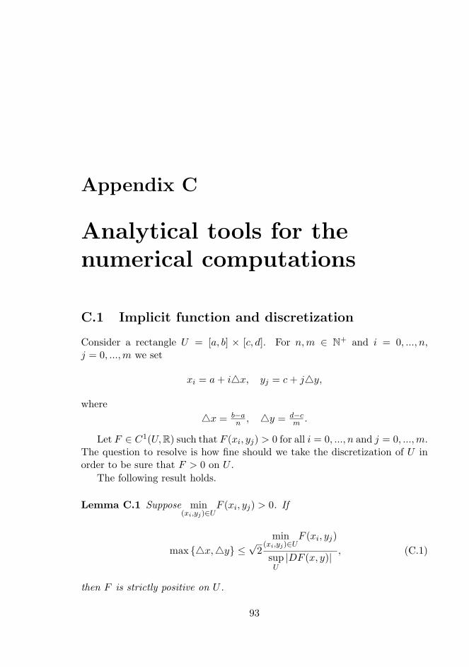
Appendix C
Analytical tools for thenumerical computations
C.1 Implicit function and discretization
Consider a rectangle U = [a, b] × [c, d]. For n,m ∈ N+ and i = 0, ..., n,j = 0, ...,m we set
xi = a+ i4x, yj = c+ j4y,
where4x = b−a
n , 4y = d−cm .
Let F ∈ C1(U,R) such that F (xi, yj) > 0 for all i = 0, ..., n and j = 0, ...,m.The question to resolve is how fine should we take the discretization of U inorder to be sure that F > 0 on U .
The following result holds.
Lemma C.1 Suppose min(xi,yj)∈U
F (xi, yj) > 0. If
max 4x,4y ≤√
2min
(xi,yj)∈UF (xi, yj)
supU|DF (x, y)|
, (C.1)
then F is strictly positive on U .
93

94APPENDIX C. ANALYTICAL TOOLS FOR THE NUMERICAL COMPUTATIONS
Proof. For every (x, y) ∈ U there is (xi, yj) with |x− xi| ≤ 124x and
|y − yj | ≤ 124y. By the mean value theorem there exists (ξ1, ξ2)∈[(x, y) , (xi, yj)]
such thatF (x, y) = F (xi, yj) +DF (ξ1, ξ2) · (x− xi, y − yj).
The following chain of estimates then holds
F (x, y) = F (xi, yj) +DF (ξ1, ξ2) · (x− xi, y − yj) ≥
≥ min(xi,yj)∈U
F (xi, yj)− supU|DF (x, y)| |(x− xi, y − yj)| ≥
≥ min(xi,yj)∈U
F (xi, yj)−√
22
supU|DF (x, y)|max 4x,4y .
This last expression is positive if (C.1) holds.
C.2 A version of the Morse theorem
Let V ⊂ R2 be open and bounded, F ∈ C∞(V,R).For the gradient of F we use DF and D2F is the Hessian matrix.
Definition C.2 A point a ∈ V is said to be a critical point of F if DF (a) = 0.Moreover, the critical point a ∈ V is said to be non-degenerate if detD2F (a) 6=0.
In order to study the level set Γ defined in subsection 3.4.1 we need theMorse theorem. The original version of the theorem reads as (see [29]):
Let V be a Banach space, O a convex neighborhood of theorigin in V and f : O → R a Ck+2 function (k ≥ 1) having theorigin as a non-degenerate critical point, with f(0) = 0. Thenthere is a neighborhood U of the origin and a Ck diffeomorphismφ : U → O with φ(0) = 0 and Dφ(0) = I, the identity map of V,such that for x ∈ U , f(φ(x)) = 1
2
(D2f(0)x, x
).
Below we give our formulation of the theorem. This formulation is moreconvenient for our purposes. We will give a constructive proof that allows usto find an explicit neighborhood of a critical point where the diffeomorphismexists.
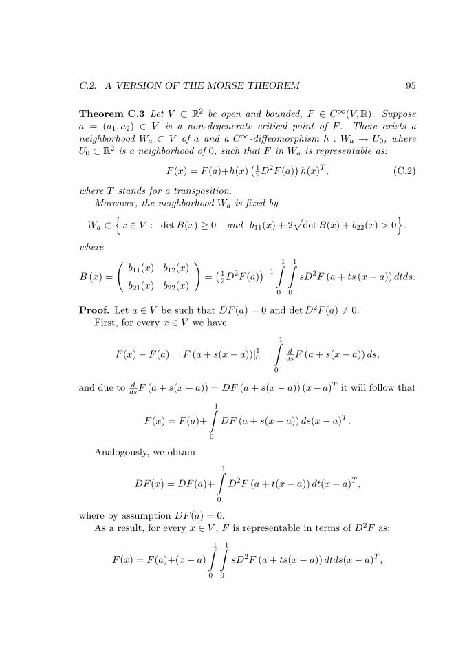
C.2. A VERSION OF THE MORSE THEOREM 95
Theorem C.3 Let V ⊂ R2 be open and bounded, F ∈ C∞(V,R). Supposea = (a1, a2) ∈ V is a non-degenerate critical point of F . There exists aneighborhood Wa ⊂ V of a and a C∞-diffeomorphism h : Wa → U0, whereU0 ⊂ R2 is a neighborhood of 0, such that F in Wa is representable as:
F (x) = F (a)+h(x)(
12D
2F (a))h(x)T , (C.2)
where T stands for a transposition.Moreover, the neighborhood Wa is fixed by
Wa ⊂x ∈ V : detB(x) ≥ 0 and b11(x) + 2
√detB(x) + b22(x) > 0
.
where
B (x) =
(b11(x) b12(x)
b21(x) b22(x)
)=(
12D
2F (a))−1
1∫0
1∫0
sD2F (a+ ts (x− a)) dtds.
Proof. Let a ∈ V be such that DF (a) = 0 and detD2F (a) 6= 0.First, for every x ∈ V we have
F (x)− F (a) = F (a+ s(x− a))|10 =
1∫0
ddsF (a+ s(x− a)) ds,
and due to ddsF (a+ s(x− a)) = DF (a+ s(x− a)) (x−a)T it will follow that
F (x) = F (a)+
1∫0
DF (a+ s(x− a)) ds(x− a)T .
Analogously, we obtain
DF (x) = DF (a)+
1∫0
D2F (a+ t(x− a)) dt(x− a)T ,
where by assumption DF (a) = 0.As a result, for every x ∈ V , F is representable in terms of D2F as:
F (x) = F (a)+(x− a)
1∫0
1∫0
sD2F (a+ ts(x− a)) dtds(x− a)T ,
96APPENDIX C. ANALYTICAL TOOLS FOR THE NUMERICAL COMPUTATIONS
or shortlyF (x) = F (a)+(x− a)K(x)(x− a)T . (C.3)
Here K(x) =∫ 10
∫ 10 sD
2F (a+ ts(x− a)) dtds is a symmetric matrix. Withthis definition, K(a) = 1
2D2F (a) is symmetric and invertible (detD2F (a) 6= 0
by assumption).Let us bring some intermediate results.1) For every x ∈ V , there exists matrix B such that
K(x) = K(a)B(x). (C.4)
Indeed, since K(a) is invertible, the matrix B(x) = K(a)−1K(x) is well-defined. We write
B(x) =
(b11(x) b12(x)
b21(x) b22(x)
),
Since F ∈ C∞(V,R), so are bij , i, j = 1, 2. Note that B(a) = I.2) Since x 7→ B(x) is C∞ in a neighborhood of a and B(a) = I, B(x) is
positive definite in a neighborhood of a, and hence allows a square root. Inparticular, it holds that
C(x) =√B(x) := 1
2πi
∮γ
√z (Iz −B(x))−1 dz, (C.5)
where γ is a Jordan curve in C which goes around the eigenvalues λ1, λ2 ∈ Cof B(x) and does not intersect Re(z) ≤ 0, Im(z) = 0.
One may check that C, defined as follows
C(x) =
b11(x)+
√detB(x)q
b11(x)+2√
detB(x)+b22(x)
b12(x)qb11(x)+2
√detB(x)+b22(x)
b21(x)qb11(x)+2
√detB(x)+b22(x)
b22(x)+√
detB(x)qb11(x)+2
√detB(x)+b22(x)
,
is indeed such thatC(x)2 = B(x). (C.6)
With this definition, C(a) = I and C(a)2 = I = B(a) as required. Also,matrix C is well defined when
detB(x) ≥ 0 and b11(x) + 2√
detB(x) + b22(x) > 0. (C.7)
C.2. A VERSION OF THE MORSE THEOREM 97
3) For those x one finds
K(a)B(x) = K(x) = K(x)K(a)−1K(a) = K(x)T(K(a)−1
)TK(a) =
=(K(a)−1K(x)
)TK(a) = BT (x)K(a).
Due to this we deduce the following
(Iz −B(x))K(a)−1 = K(a)−1 (Iz −B(x))T ,
and hence
K(a) (Iz −B(x))−1 =((Iz −B(x))K(a)−1
)−1 =
=(K(a)−1 (Iz −B(x))T
)−1=((Iz −B(x))T
)−1K(a) =
=((Iz −B(x))−1
)TK(a).
Applying the integration (C.5) to the last identity we find
K(a)C(x) = C(x)TK(a). (C.8)
Combining (C.4), (C.6) and (C.8) we have
K(x) = K(a)B(x) = K(a)C(x)2 = C(x)TK(a)C(x),
and therefore (C.3) for those x results in
F (x) = F (a) + F (a)+h(x)K(a)h(x)T , (C.9)
where K(a) = 12D
2F (a) and
h(x)T = C(x)(x− a)T .
Note that by (C.7) the representation for F in (C.9) holds on a set Wa ⊂ Vwhich is star-shaped with respect to a and such that
Wa ⊂x ∈ V : detB(x) ≥ 0 and b11(x) + 2
√detB(x) + b22(x) > 0
.
(C.10)
Remark C.4 For each pair (F, a) one can obtain an explicit estimate for Wa
in (C.10). We will do this in the next subsection for the pair we are interestedin.
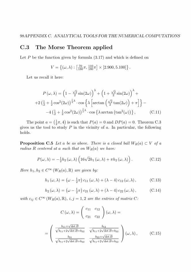
98APPENDIX C. ANALYTICAL TOOLS FOR THE NUMERICAL COMPUTATIONS
C.3 The Morse Theorem applied
Let P be the function given by formula (3.17) and which is defined on
V =(ω, λ) :
[70180π,
110180π
]× [2.900, 5.100]
.
Let us recall it here:
P (ω, λ) =(1−
√2
2 sin(2ω))λ
+(1 +
√2
2 sin(2ω))λ
+
+2(
12 + 1
2 cos2(2ω)) 1
2λ · cos
λ[arctan
(√2
2 tan(2ω))
+ π]−
−4(
12 + 1
2 cos2(2ω)) 1
2λ · cos
λ arctan
(tan2(ω)
), (C.11)
The point a =(
12π, 4
)is such that P (a) = 0 and DP (a) = 0. Theorem C.3
gives us the tool to study P in the vicinity of a. In particular, the followingholds.
Proposition C.5 Let a be as above. There is a closed ball WR(a) ⊂ V of aradius R centered at a such that on WR(a) we have:
P (ω, λ) = −12h2 (ω, λ)
(16√
2h1 (ω, λ) + πh2 (ω, λ)). (C.12)
Here h1, h2 ∈ C∞ (WR(a),R) are given by:
h1 (ω, λ) =(ω − 1
2π)c11 (ω, λ) + (λ− 4) c12 (ω, λ) , (C.13)
h2 (ω, λ) =(ω − 1
2π)c21 (ω, λ) + (λ− 4) c22 (ω, λ) , (C.14)
with cij ∈ C∞ (WR(a),R), i, j = 1, 2 are the entries of matrix C:
C (ω, λ) =
(c11 c12
c21 c22
)(ω, λ) =
=
b11+
√detB√
b11+2√
detB+b22
b12√b11+2
√detB+b22
b21√b11+2
√detB+b22
b22+√
detB√b11+2
√detB+b22
(ω, λ) , (C.15)
C.3. THE MORSE THEOREM APPLIED 99
while bij ∈ C∞(V,R), i, j = 1, 2 are as follows
B (ω, λ) =
(b11 b12
b21 b22
)(ω, λ) =
=(
12D
2P (a))−1
1∫0
1∫0
sD2P (a+ ts ((ω, λ)− a)) dtds. (C.16)
Note that B(a) = I and C(a) = I.The ball WR(a) is fixed by
WR(a) :=(ω, λ) ∈ V :
∣∣(ω − 12π, λ− 4
)∣∣ ≤ R, (C.17)
with R = − 1120π
2 −√
218 π + 1
120π√π2 + 40
3
√2π + 1568
9 ≈ 0.078 (In the ω-direction we have that R ≈ 4.5).
C.3.1 Computational results I
It is straightforward for a =(
12π, 4
)that
∂2P∂ω2 (a) = 0, ∂2P
∂ω∂λ(a) = −8√
2π, ∂2P∂λ2 (a) = −π2, (C.18)
and hencedetD2P (a) = −128π2. (C.19)
To simplify the notations, we use x instead of (ω, λ) when (ω, λ) standsfor a argument.
Now let us bring two alternatives representations for the entries of matrixB given by (C.16), which we will use later on.
Representation I We will need the explicit formula for the coefficients bij ,i, j = 1, 2. Let us find them in a straightforward way from (C.16).
We write down the integral term1∫0
1∫0
sD2P (a+ ts (x− a)) dtds in (C.16)
as follows
1∫0
1∫0
sD2P (a+ ts (x− a)) dtds =
(r1(x) r2(x)
r2(x) r3(x)
), (C.20)
100APPENDIX C. ANALYTICAL TOOLS FOR THE NUMERICAL COMPUTATIONS
where rj , j = 1, 2, 3 read as:
r1(x) =
1∫0
1∫0
s∂2P∂ω2 (a+ ts(x− a))dtds, (C.21)
r2(x) =
1∫0
1∫0
s ∂2P
∂ω∂λ(a+ ts(x− a))dtds, (C.22)
r3(x) =
1∫0
1∫0
s∂2P∂λ2 (a+ ts(x− a))dtds. (C.23)
Then the entries bij , i, j = 1, 2 of matrix B in terms of rj , j = 1, 2, 3 anddue to (C.18), (C.19) will read:
b11(x) = 2detD2P (a)
(∂2P∂λ2 (a)r1(x)− ∂2P
∂ω∂λ(a)r2(x))
= 164r1(x)−
√2
8π r2(x),(C.24)
b12(x) = 2detD2P (a)
(∂2P∂λ2 (a)r2(x)− ∂2P
∂ω∂λ(a)r3(x))
= 164r2(x)−
√2
8π r3(x),(C.25)
b21(x) = 2detD2P (a)
(∂2P∂ω2 (a)r2(x)− ∂2P
∂ω∂λ(a)r1(x))
= −√
28π r1(x), (C.26)
b22(x) = 2detD2P (a)
(∂2P∂ω2 (a)r3(x)− ∂2P
∂ω∂λ(a)r2(x))
= −√
28π r2(x). (C.27)
Representation II On the other hand, let us obtain for rj , j = 1, 2, 3 thefollowing representations:
r1(x) = 12∂2P∂ω2 (a) + q1(x),
r2(x) = 12∂2P∂ω∂λ(a) + q2(x),
r3(x) = 12∂2P∂λ2 (a) + q3(x),
whereq1(x) =
=
1∫0
1∫0
1∫0
ts2(∂3P∂ω3 (a+ tsσ(x− a)), ∂3P
∂ω2∂λ(a+ tsσ(x− a))
)(x− a)Tdσdtds,
(C.28)
C.3. THE MORSE THEOREM APPLIED 101
q2(x) =
=
1∫0
1∫0
1∫0
ts2(
∂3P∂ω2∂λ
(a+ tsσ(x− a)), ∂3P∂ω∂λ2 (a+ tsσ(x− a))
)(x−a)Tdσdtds,
(C.29)q3(x) =
=
1∫0
1∫0
1∫0
ts2(
∂3P∂ω∂λ2 (a+ tsσ(x− a)), ∂
3P∂λ3 (a+ tsσ(x− a))
)(x− a)Tdσdtds.
(C.30)This will yield another representation formulas for bij , i, j = 1, 2 of matrix
B, namely,
b11(x) = 1+ 2detD2P (a)
(∂2P∂λ2 (a)q1(x)− ∂2P
∂ω∂λ(a)q2(x))
= 1+ 164q1(x)−
√2
8π q2(x),(C.31)
b12(x) = 2detD2P (a)
(∂2P∂λ2 (a)q2(x)− ∂2P
∂ω∂λ(a)q3(x))
= 164q2(x)−
√2
8π q3(x),(C.32)
b21(x) = 2detD2P (a)
(∂2P∂ω2 (a)q2(x)− ∂2P
∂ω∂λ(a)q1(x))
= −√
28π q1(x), (C.33)
b22(x) = 1 + 2detD2P (a)
(∂2P∂ω2 (a)q3(x)− ∂2P
∂ω∂λ(a)q2(x))
= 1−√
28π q2(x). (C.34)
This representation, together with the estimates from above for |qj | , j =1, 2, 3 on V given below, will be useful in the proof of Proposition C.5.
Estimates for |qj | , j = 1, 2, 3 on V Let qj , j = 1, 2, 3 by given by (C.28) –(C.30). We will need the estimates for |qj | , j = 1, 2, 3 on V . Let us also usethe notations ∂3P
∂(ω,λ)αj ,∂3P
∂(ω,λ)βjfor the corresponding differentiations in each qj ,
j = 1, 2, 3. For example for q1 it will be ∂3P∂(ω,λ)αj = ∂3P
∂ω3 and ∂3P
∂(ω,λ)βj= ∂3P
∂ω2∂λ,
etc. For every qj , j = 1, 2, 3 we then in general have:
|qj(x)| =
∣∣∣∣∣∣1∫
0
1∫0
1∫0
ts2(
∂3P∂(ω,λ)αj (a+ tsσ(x− a)),
∂3P
∂(ω,λ)βj(a+ tsσ(x− a))
)(x− a)Tdσdtds
∣∣∣ ≤
102APPENDIX C. ANALYTICAL TOOLS FOR THE NUMERICAL COMPUTATIONS
≤1∫
0
1∫0
1∫0
ts2 supx∈V
∣∣∣( ∂3P∂(ω,λ)αj (x), ∂3P
∂(ω,λ)βj(x))∣∣∣ dσdtds |x− a| =
= 16 supx∈V
∣∣∣( ∂3P∂(ω,λ)αj (x), ∂3P
∂(ω,λ)βj(x))∣∣∣ |x− a| ≤Mj |x− a| . (C.35)
where Mj is an upper bound for function 16
∣∣∣( ∂3P∂(ω,λ)αj (x), ∂3P
∂(ω,λ)βj(x))∣∣∣ on V .
In particular, one shows by explicit and tedious computations that for
M1 = 180, M2 = 75, M3 = 30,
the estimate (C.35) for the corresponding |qj |, j = 1, 2, 3 holds true. We depictthe results in Table C.1.
|q1(x)| < 180 |x− a| |q2(x)| < 75 |x− a| |q3(x)| < 30 |x− a|
Table C.1: Estimates from above for |qj | , j = 1, 2, 3 on V
Now we proceed with a proof of Proposition C.5.
C.3.2 Checking the range for Morse
Proof of Proposition C.5. Representation (C.12) is a consequence ofTheorem C.3. It is straightforward for a =
(12π, 4
)that P (a) = 0. We also
find that DP (a) = 0, meaning a is a critical point of P . Due to (C.19) weconclude that a is a non-degenerate critical point of P .
By Theorem C.3 in a vicinity Wa ⊂ V of a which is defined in (C.10), weobtain
P (x) = (h1(x), h2(x)) · 12D
2P (a) · (h1(x), h2(x))T =
= −12h2 (x)
(16√
2h1 (x) + πh2 (x)), (C.36)
where h1, h2 ∈ C∞ (Wa,R). Their explicit formulas read as (C.13), (C.14).We show that Wa in our case can be taken as a closed ball WR(a) centered
at a of radius R and the numerical approximation for its range is given by(C.17). We will do this in two steps.
1) Let us solve the inequality detB(x) ≥ 0 on V .Due to (C.31) – (C.34) we will get
detB(x) = b11(x)b22(x)− b12(x)b21(x) =
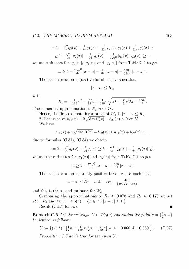
C.3. THE MORSE THEOREM APPLIED 103
= 1−√
24π q2(x) + 1
64q1(x)−1
32π2 q1(x)q3(x) + 132π2 q
22(x) ≥
≥ 1−√
24π |q2(x)| −
164 |q1(x)| −
132π2 |q1(x)| |q3(x)| ≥ ...
we use estimates for |q1(x)|, |q2(x)| and |q3(x)| from Table C.1 to get
... ≥ 1− 75√
24π |x− a| − 180
64 |x− a| − 540032π2 |x− a|2 .
The last expression is positive for all x ∈ V such that
|x− a| ≤ R1,
withR1 = − 1
120π2 −
√2
18 π + 1120π
√π2 + 40
3
√2π + 1568
9 .
The numerical approximation is R1 ≈ 0.078.Hence, the first estimate for a range of Wa is |x− a| ≤ R1.2) Let us solve b11(x) + 2
√detB(x) + b22(x) > 0 on V .
We have
b11(x) + 2√
detB(x) + b22(x) ≥ b11(x) + b22(x) = ...
due to formulas (C.31), (C.34) we obtain
... = 2−√
24π q2(x) + 1
64q1(x) ≥ 2−√
24π |q2(x)| −
164 |q1(x)| ≥ ...
we use the estimates for |q1(x)| and |q2(x)| from Table C.1 to get
... ≥ 2− 75√
24π |x− a| − 180
64 |x− a| .
The last expression is strictly positive for all x ∈ V such that
|x− a| < R2 with R2 = 32π
(300√
2+45π) ,
and this is the second estimate for Wa.Comparing the approximations to R1 ≈ 0.078 and R2 ≈ 0.178 we set
R := R1 and Wa := WR(a) = x ∈ V : |x− a| ≤ R.Result (C.17) follows.
Remark C.6 Let the rectangle U ⊂ WR(a) containing the point a =(
12π, 4
)be defined as follows:
U :=(ω, λ) :
[12π −
2180π,
12π + 2
180π]× [4− 0.060, 4 + 0.060]
. (C.37)
Proposition C.5 holds true for the given U .
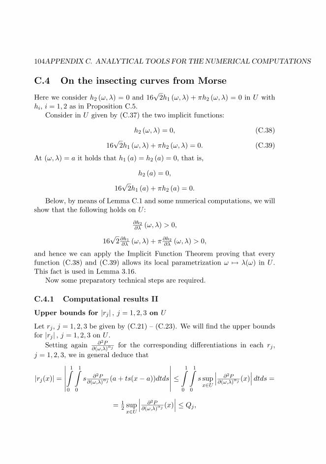
104APPENDIX C. ANALYTICAL TOOLS FOR THE NUMERICAL COMPUTATIONS
C.4 On the insecting curves from Morse
Here we consider h2 (ω, λ) = 0 and 16√
2h1 (ω, λ) + πh2 (ω, λ) = 0 in U withhi, i = 1, 2 as in Proposition C.5.
Consider in U given by (C.37) the two implicit functions:
h2 (ω, λ) = 0, (C.38)
16√
2h1 (ω, λ) + πh2 (ω, λ) = 0. (C.39)
At (ω, λ) = a it holds that h1 (a) = h2 (a) = 0, that is,
h2 (a) = 0,
16√
2h1 (a) + πh2 (a) = 0.
Below, by means of Lemma C.1 and some numerical computations, we willshow that the following holds on U :
∂h2∂λ (ω, λ) > 0,
16√
2∂h1∂λ (ω, λ) + π ∂h2
∂λ (ω, λ) > 0,
and hence we can apply the Implicit Function Theorem proving that everyfunction (C.38) and (C.39) allows its local parametrization ω 7→ λ(ω) in U .This fact is used in Lemma 3.16.
Now some preparatory technical steps are required.
C.4.1 Computational results II
Upper bounds for |rj | , j = 1, 2, 3 on U
Let rj , j = 1, 2, 3 be given by (C.21) – (C.23). We will find the upper boundsfor |rj | , j = 1, 2, 3 on U .
Setting again ∂2P∂(ω,λ)αj for the corresponding differentiations in each rj ,
j = 1, 2, 3, we in general deduce that
|rj(x)| =
∣∣∣∣∣∣1∫
0
1∫0
s ∂2P∂(ω,λ)αj (a+ ts(x− a))dtds
∣∣∣∣∣∣ ≤1∫
0
1∫0
s supx∈U
∣∣∣ ∂2P∂(ω,λ)αj (x)
∣∣∣ dtds =
= 12 supx∈U
∣∣∣ ∂2P∂(ω,λ)αj (x)
∣∣∣ ≤ Qj ,

C.4. ON THE INSECTING CURVES FROM MORSE 105
where Qj , j = 1, 2, 3 is an upper bound for the function 12
∣∣∣ ∂2P∂(ω,λ)αj (x)
∣∣∣ on U .
In analogous way we find the upper bounds for∣∣∣∂rj∂ω
∣∣∣, ∣∣∣∂rj∂λ ∣∣∣ and∣∣∣ ∂2rj∂ω∂λ
∣∣∣,∣∣∣∂2rj∂λ2
∣∣∣, j = 1, 2, 3 on U , we will need later on. Explicit bounds are given in
Table C.2. Note that we skip the derivatives ∂2rj∂ω2 since there will be no need
for them.
|r1(x)| < 5
∣∣∣∂r1∂ω (x)∣∣∣ < 43∣∣∣∂r1∂λ (x)∣∣∣ < 25
∣∣∣ ∂2r1∂ω∂λ(x)
∣∣∣ < 175∣∣∣∂2r1∂λ2 (x)
∣∣∣ < 65
|r2(x)| < 19
∣∣∣∂r2∂ω (x)∣∣∣ < 25∣∣∣∂r2∂λ (x)∣∣∣ < 6
∣∣∣ ∂2r2∂ω∂λ(x)
∣∣∣ < 65∣∣∣∂2r2∂λ2 (x)
∣∣∣ < 33
|r3(x)| < 6
∣∣∣∂r3∂ω (x)∣∣∣ < 6∣∣∣∂r3∂λ (x)∣∣∣ < 4
∣∣∣ ∂2r3∂ω∂λ(x)
∣∣∣ < 33∣∣∣∂2r3∂λ2 (x)
∣∣∣ < 16
Table C.2: Estimates from above for the absolute value of rj, j = 1, 2, 3 andsome higher order derivatives on U
Upper bounds for |qj | , j = 1, 2, 3 on U
Let qj , j = 1, 2, 3 be given by (C.28) – (C.30).Earlier we found the estimates for |qj | , j = 1, 2, 3 on V of the type |qj | ≤
Mj |x− a| , j = 1, 2, 3 (see Table C.1). Here, we will obtain the constantswhich are the upper bounds for |qj | , j = 1, 2, 3 on U .
Setting ∂3P∂(ω,λ)αj ,
∂3P
∂(ω,λ)βjfor the corresponding differentiations in each qj ,
j = 1, 2, 3, analogously to (C.35), we have that
|qj(x)| =
∣∣∣∣∣∣1∫
0
1∫0
1∫0
ts2(
∂3P∂(ω,λ)αj (a+ tsσ(x− a)),
∂3P
∂(ω,λ)βj(a+ tsσ(x− a))
)(x− a)Tdσdtds
∣∣∣ ≤
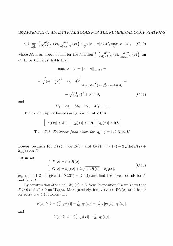
106APPENDIX C. ANALYTICAL TOOLS FOR THE NUMERICAL COMPUTATIONS
≤ 16 supx∈U
∣∣∣( ∂3P∂(ω,λ)αj (x), ∂3P
∂(ω,λ)βj(x))∣∣∣max
U|x− a| ≤Mj max
U|x− a| , (C.40)
where Mj is an upper bound for the function 16
∣∣∣( ∂3P∂(ω,λ)αj (x), ∂3P
∂(ω,λ)βj(x))∣∣∣ on
U . In particular, it holds that
maxU|x− a| = |x− a||on ∂U =
=√(
ω − 12π)2 + (λ− 4)2
∣∣∣∣at (ω,λ)=
12π−
2180π,4−0.060
=
=√(
190π)2 + 0.0602, (C.41)
andM1 = 44, M2 = 27, M3 = 11.
The explicit upper bounds are given in Table C.3.
|q1(x)| < 3.1 |q2(x)| < 1.9 |q3(x)| < 0.8
Table C.3: Estimates from above for |qj |, j = 1, 2, 3 on U
Lower bounds for F (x) = detB(x) and G(x) = b11(x) + 2√
detB(x) +b22(x) on U
Let us set F (x) = detB(x),
G(x) = b11(x) + 2√
detB(x) + b22(x),(C.42)
bij , i, j = 1, 2 are given in (C.31) – (C.34) and find the lower bounds for Fand G on U .
By construction of the ball WR(a) ⊃ U from Proposition C.5 we know thatF ≥ 0 and G > 0 on WR(a). More precisely, for every x ∈ WR(a) (and hencefor every x ∈ U) it holds that
F (x) ≥ 1−√
24π |q2(x)| −
164 |q1(x)| −
132π2 |q1(x)| |q3(x)| ,
andG(x) ≥ 2−
√2
4π |q2(x)| −164 |q1(x)| .

C.4. ON THE INSECTING CURVES FROM MORSE 107
Due to results of Table C.3 we finally obtain that on UF (x) ≥ 0.730... > 0.7,
G(x) ≥ 1.738... > 1.7.(C.43)
Upper bounds for |bij |, i, j = 1, 2 on U
Let bij , i, j = 1, 2 be given by (C.24) – (C.27), namely,
b11(x) = 164r1(x)−
√2
8π r2(x),
b12(x) = 164r2(x)−
√2
8π r3(x),
b21(x) = −√
28π r1(x),
b22(x) = −√
28π r2(x),
with rj , j = 1, 2, 3 as in (C.21) – (C.23).Using the results of Table C.2 we will find the following upper bounds for
the absolute values of bij , i, j = 1, 2 and some higher order derivatives on U(see Table C.4).
Upper bounds for F (x) = detB(x) and G(x) = b11(x) + 2√
detB(x) +b22(x) on U
Recall that F and G are given by (C.42). They are positive functions on Uwith lower bounds as in (C.43). Here we find their upper bounds togetherwith the upper bounds for some higher order derivatives.
In particular, in order to obtain the estimates for F ,∣∣∂F∂ω
∣∣, ∣∣∂F∂λ ∣∣ and∣∣∣ ∂2F∂ω∂λ
∣∣∣,∣∣∣∂2F∂λ2
∣∣∣ on U , we use the results of Table C.4. The estimates found are presentedin the first row of Table C.5.
In order to find the estimates for∣∣∂G∂ω
∣∣ , ∣∣∂G∂λ ∣∣ and∣∣∣ ∂2G∂ω∂λ
∣∣∣ , ∣∣∣∂2G∂λ2
∣∣∣ we use- the lower bound for Fon U , namely, F (x) > 0.7,- the results of Table C.4 and- the results from the first row of Table C.5.E.g. for
∣∣∂G∂ω
∣∣ we will have that on U
∣∣∂G∂ω (x)
∣∣ = ∣∣∣∣∂b11∂ω (x) +∂F∂ω (x)√F (x)
+ ∂b22∂ω (x)
∣∣∣∣ ≤

108APPENDIX C. ANALYTICAL TOOLS FOR THE NUMERICAL COMPUTATIONS
|b11(x)| < 1.2
∣∣∣∂b11∂ω (x)∣∣∣ < 2.1∣∣∣∂b11∂λ (x)∣∣∣ < 0.8
∣∣∣∂2b11∂ω∂λ(x)
∣∣∣ < 6.4∣∣∣∂2b11∂λ2 (x)
∣∣∣ < 2.9
|b12(x)| < 0.7
∣∣∣∂b12∂ω (x)∣∣∣ < 0.8∣∣∣∂b12∂λ (x)∣∣∣ < 0.4
∣∣∣∂2b12∂ω∂λ(x)
∣∣∣ < 2.9∣∣∣∂2b12∂λ2 (x)
∣∣∣ < 1.5
|b21(x)| < 0.3
∣∣∣∂b21∂ω (x)∣∣∣ < 2.5∣∣∣∂b21∂λ (x)∣∣∣ < 1.5
∣∣∣∂2b21∂ω∂λ(x)
∣∣∣ < 9.9∣∣∣∂2b21∂λ2 (x)
∣∣∣ < 3.7
|b22(x)| < 1.1
∣∣∣∂b22∂ω (x)∣∣∣ < 1.5∣∣∣∂b22∂λ (x)∣∣∣ < 0.4
∣∣∣∂2b22∂ω∂λ(x)
∣∣∣ < 3.7∣∣∣∂2b22∂λ2 (x)
∣∣∣ < 1.9
Table C.4: Estimates from above for the absolute value of bij, i, j = 1, 2 andsome higher order derivatives on U
≤ supU
∣∣∣∂b11∂ω (x)∣∣∣+ sup
U
∂F∂ω (x)
infU
√F (x)
+ supU
∣∣∣∂b22∂ω (x)∣∣∣ <
< 2.1 + 6.1√0.7
+ 1.5 ≈ 10.891 < 11.
The other estimates on U for the derivatives of G listed above are obtained inan analogous way and presented in Table C.5.
F (x) < 1.53
∣∣∂F∂ω (x)
∣∣ < 6.10∣∣∂F∂λ (x)
∣∣ < 2.53
∣∣∣ ∂2F∂ω∂λ(x)
∣∣∣ < 23.52∣∣∣∂2F∂λ2 (x)
∣∣∣ < 10.35
−
∣∣∂G∂ω (x)
∣∣ < 11∣∣∂G∂λ (x)
∣∣ < 4.3
∣∣∣ ∂2G∂ω∂λ(x)
∣∣∣ < 51.4∣∣∣∂2G∂λ2 (x)
∣∣∣ < 22.7
Table C.5: Estimates from above for F and G on U
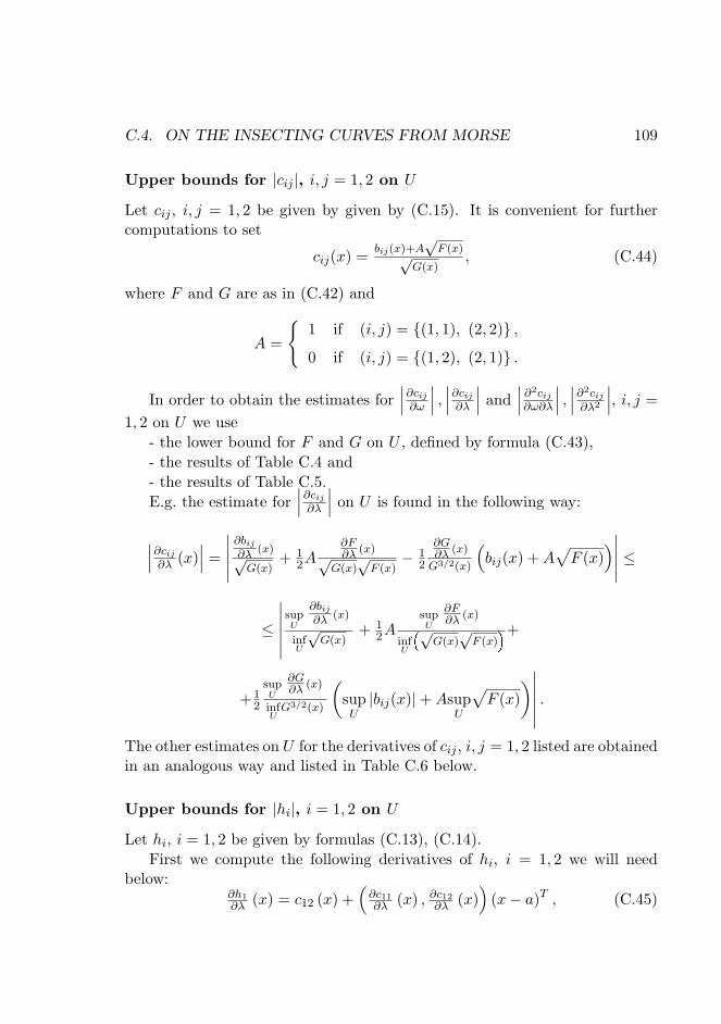
C.4. ON THE INSECTING CURVES FROM MORSE 109
Upper bounds for |cij |, i, j = 1, 2 on U
Let cij , i, j = 1, 2 be given by given by (C.15). It is convenient for furthercomputations to set
cij(x) = bij(x)+A√F (x)√
G(x), (C.44)
where F and G are as in (C.42) and
A =
1 if (i, j) = (1, 1), (2, 2) ,
0 if (i, j) = (1, 2), (2, 1) .
In order to obtain the estimates for∣∣∣∂cij∂ω
∣∣∣ , ∣∣∣∂cij∂λ
∣∣∣ and∣∣∣ ∂2cij∂ω∂λ
∣∣∣ , ∣∣∣∂2cij∂λ2
∣∣∣, i, j =1, 2 on U we use
- the lower bound for F and G on U , defined by formula (C.43),- the results of Table C.4 and- the results of Table C.5.E.g. the estimate for
∣∣∣∂cij∂λ
∣∣∣ on U is found in the following way:
∣∣∣∂cij∂λ (x)∣∣∣ = ∣∣∣∣∣ ∂bij∂λ (x)√
G(x)+ 1
2A∂F∂λ (x)√
G(x)√F (x)
− 12
∂G∂λ (x)
G3/2(x)
(bij(x) +A
√F (x)
)∣∣∣∣∣ ≤≤
∣∣∣∣∣∣supU
∂bij∂λ (x)
infU
√G(x)
+ 12A
supU
∂F∂λ (x)
infU
√G(x)
√F (x)
+
+12
supU
∂G∂λ (x)
infUG3/2(x)
(supU|bij(x)|+Asup
U
√F (x)
)∣∣∣∣∣∣ .The other estimates on U for the derivatives of cij , i, j = 1, 2 listed are obtainedin an analogous way and listed in Table C.6 below.
Upper bounds for |hi|, i = 1, 2 on U
Let hi, i = 1, 2 be given by formulas (C.13), (C.14).First we compute the following derivatives of hi, i = 1, 2 we will need
below:∂h1∂λ (x) = c12 (x) +
(∂c11∂λ (x) , ∂c12∂λ (x)
)(x− a)T , (C.45)
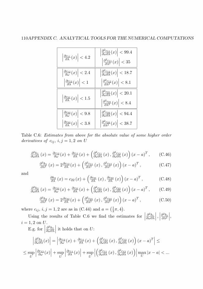
110APPENDIX C. ANALYTICAL TOOLS FOR THE NUMERICAL COMPUTATIONS
∣∣∣∂c11∂λ (x)∣∣∣ < 4.2
∣∣∣∂2c11∂ω∂λ (x)
∣∣∣ < 99.4∣∣∣∂2c11∂λ2 (x)
∣∣∣ < 35∣∣∣∂c12∂ω (x)∣∣∣ < 2.4∣∣∣∂c12∂λ (x)∣∣∣ < 1
∣∣∣∂2c12∂ω∂λ (x)
∣∣∣ < 18.7∣∣∣∂2c12∂λ2 (x)
∣∣∣ < 8.1
∣∣∣∂c21∂λ (x)∣∣∣ < 1.5
∣∣∣∂2c21∂ω∂λ (x)
∣∣∣ < 20.1∣∣∣∂2c21∂λ2 (x)
∣∣∣ < 8.4∣∣∣∂c22∂ω (x)∣∣∣ < 9.8∣∣∣∂c22∂λ (x)∣∣∣ < 3.8
∣∣∣∂2c22∂ω∂λ (x)
∣∣∣ < 94.4∣∣∣∂2c22∂λ2 (x)
∣∣∣ < 38.7
Table C.6: Estimates from above for the absolute value of some higher orderderivatives of cij, i, j = 1, 2 on U
∂2h1∂ω∂λ (x) = ∂c12
∂ω (x) + ∂c11∂λ (x) +
(∂2c11∂ω∂λ (x) , ∂
2c12∂ω∂λ (x)
)(x− a)T , (C.46)
∂2h1∂λ2 (x) = 2∂c12∂λ (x) +
(∂2c11∂λ2 (x) , ∂
2c12∂λ2 (x)
)(x− a)T , (C.47)
and∂h2∂λ (x) = c22 (x) +
(∂c21∂λ (x) , ∂c22∂λ (x)
)(x− a)T , (C.48)
∂2h2∂ω∂λ (x) = ∂c22
∂ω (x) + ∂c21∂λ (x) +
(∂2c21∂ω∂λ (x) , ∂
2c22∂ω∂λ (x)
)(x− a)T , (C.49)
∂2h2∂λ2 (x) = 2∂c22∂λ (x) +
(∂2c21∂λ2 (x) , ∂
2c22∂λ2 (x)
)(x− a)T , (C.50)
where cij , i, j = 1, 2 are as in (C.44) and a =(
12π, 4
).
Using the results of Table C.6 we find the estimates for∣∣∣ ∂2hi∂ω∂λ
∣∣∣ , ∣∣∣∂2hi∂λ2
∣∣∣,i = 1, 2 on U .
E.g. for∣∣∣ ∂2h1∂ω∂λ
∣∣∣ it holds that on U :∣∣∣ ∂2h1∂ω∂λ(x)
∣∣∣ = ∣∣∣∂c12∂ω (x) + ∂c11∂λ (x) +
(∂2c11∂ω∂λ (x) , ∂
2c12∂ω∂λ (x)
)(x− a)T
∣∣∣ ≤≤ sup
U
∣∣∣∂c12∂ω (x)∣∣∣+ sup
U
∣∣∣∂c11∂λ (x)∣∣∣+ sup
U
∣∣∣(∂2c11∂ω∂λ (x) , ∂
2c12∂ω∂λ (x)
)∣∣∣maxU|x− a| < ...

C.4. ON THE INSECTING CURVES FROM MORSE 111
for maxU |x− a| see formula (C.41) and then
... < 2.4 + 4.2 +√
99.42 + 18.72
√(190π)2 + 0.0602 ≈ 13.621 < 13.7.
Analogously, the other estimates on U are obtained (see Table C.7).∣∣∣ ∂2h1∂ω∂λ(x)
∣∣∣ < 13.7∣∣∣ ∂2h2∂ω∂λ(x)
∣∣∣ < 18∣∣∣∂2h1∂λ2 (x)
∣∣∣ < 4.5∣∣∣∂2h2∂λ2 (x)
∣∣∣ < 10.4
Table C.7: Estimates from above for the absolute value of some higher orderderivatives of hi, i = 1, 2 on U
C.4.2 Strict positivity of the functions ∂h2
∂λ(ω, λ) and
16√
2∂h1
∂λ(ω, λ) + π ∂h2
∂λ(ω, λ) on U
Let us fix the notations which are common for two lemmas.
Notation C.7 Let U be as in (C.37), namely,
U :=(ω, λ) :
[88180π,
92180π
]× [3.940, 4.060]
.
By (ωi, λj) i=0,...,nj=0,...,m
we mean a discretization of U which is defined as
followsωi = 88
180π + i4ω, λj = 3.94 + j4λ,
with
4ω =4
180π
n , 4λ = 0.12m .
Then we deduce the following two results.
Lemma C.8 It holds that
∂h2∂λ (ω, λ) > 0 on U. (C.51)
Proof. Fix n = m = 2 and consider the discretization (ωi, λj)i=0,...,2j=0,...,2
of U
given by Notation C.7.
112APPENDIX C. ANALYTICAL TOOLS FOR THE NUMERICAL COMPUTATIONS
By straightforward computations it holds that
∂h2∂λ (ωi, λj) > 0, (C.52)
for all i = 0, ..., 2, j = 0, ..., 2 and, moreover,
min(ωi,λj)∈U
∂h2∂λ (ωi, λj) = ∂h2
∂λ (ω0, λ0) ≈ 0.952. (C.53)
Next to this, we compute
a1 = max 4ω,4λ = max 4
180π
n , 0.12m
= 0.12
2 = 0.060,
and, by taking into account the results of Table C.7 and (C.53), we also find
a2 =√
2min
(ωi,λj)∈U∂h2∂λ (ωi, λj)
supU
∣∣∣( ∂2h2∂ω∂λ(ω, λ), ∂
2h2∂λ2 (ω, λ)
)∣∣∣ ≈ 0.065.
Since a1 < a2, by Lemma C.1 we conclude that the constructed discretiza-tion (ωi, λj)i=0,...,2
j=0,...,2of U to be appropriate in the sense that condition (C.52)
yields a strict positivity of ∂h2∂λ (ω, λ) on U .
Lemma C.9 Let U be as in (C.37). It holds that
16√
2∂h1∂λ (ω, λ) + π ∂h2
∂λ (ω, λ) > 0 on U. (C.54)
Proof. Fix n = 7, m = 12 and consider the discretization (ωi, λj) i=0,...,7j=0,...,12
of U given by Notation C.7.By straightforward computations it holds that
16√
2∂h1∂λ (ωi, λj) + π ∂h2
∂λ (ωi, λj) > 0, (C.55)
for all i = 0, ..., 7, j = 0, ..., 12 and, moreover,
min(ωi,λj)∈U
(16√
2∂h1∂λ (ωi, λj) + π ∂h2
∂λ (ωi, λj))
=
= 16√
2∂h1∂λ (ω0, λ0) + π ∂h2
∂λ (ω0, λ0) ≈ 2.936. (C.56)
C.5. ON P (ω, λ) = 0 IN V AWAY FROM A =(
12π, 4
)113
Next to this, we compute
b1 = max 4ω,4λ = max 4
180π
n , 0.12m
= 0.12
12 = 0.010,
and, by taking into account the results of Table C.7 and (C.56), we also find
b2 =
=
√2 min(ωi,λj)∈U
(16√
2∂h1∂λ (ωi, λj) + π ∂h2
∂λ (ωi, λj))
supU
∣∣∣(16√
2 ∂2h1
∂ω∂λ(ω, λ) + π ∂2h2∂ω∂λ(ω, λ), 16
√2∂
2h1∂λ2 (ω, λ) + π ∂
2h2∂λ2 (ω, λ)
)∣∣∣ ≈≈ 0.011.
Since b1 < b2, by Lemma C.1 we conclude that the constructed discretiza-tion (ωi, λj) i=0,...,7
j=0,...,12of U to be appropriate in the sense that condition (C.55)
yields a strict positivity of 16√
2∂h1∂λ (ω, λ) + π ∂h2
∂λ (ω, λ) on U .
C.5 On P (ω, λ) = 0 in V away from a =(1
2π, 4)
Recall here function P defined on V =(ω, λ) :
[70180π,
110180π
]× [2.900, 5.100]
:
P (ω, λ) =(1−
√2
2 sin(2ω))λ
+(1 +
√2
2 sin(2ω))λ
+
+2(
12 + 1
2 cos2(2ω)) 1
2λ · cos
λ[arctan
(√2
2 tan(2ω))
+ π]−
−4(
12 + 1
2 cos2(2ω)) 1
2λ · cos
λ arctan
(tan2(ω)
), (C.57)
C.5.1 Set of Claims I
In a set of claims below we describe some properties of the first derivatives ∂P∂ω
and ∂P∂λ on V away from the point a =
(12π, 4
)which are used in Lemma 3.16.
Claim C.10 Let H1 ⊂ V be as follows
H1 =(ω, λ) :
[84180π,
90180π
]× [4.030, 4.970]
.
It holds that ∂P∂ω (ω, λ) < 0 on H1.
114APPENDIX C. ANALYTICAL TOOLS FOR THE NUMERICAL COMPUTATIONS
Proof. First we find the following estimates:∣∣∣∂2P∂ω2 (ω, λ)
∣∣∣ < 162,∣∣∣ ∂2P∂ω∂λ(ω, λ)
∣∣∣ < 45 on H1. (C.58)
Then we fix n = 14, m = 120 and consider the discretization(ωi, λj) i=0,14
j=0,...,120of H1 such that
ωi = 84180π + i4ω, λj = 4.030 + j4λ,
with
4ω =6
180π
n , 4λ = 0.94m .
By straightforward computations it holds that
− ∂P∂ω (ωi, λj) > 0, (C.59)
for all i = 0, ..., 14, j = 0, ..., 120 and, moreover,
min(ωi,λj)∈H1
(−∂P∂ω (ωi, λj)
)= −∂P
∂ω (ω9, λ0) ≈ 1.022. (C.60)
Next to this, we compute
c1 = max 4ω,4λ = max 6
180π
n , 0.94m
= 0.94
120 ≈ 0.00783,
and, by taking into account (C.58) and (C.60), we also find
c2 =√
2min
(ωi,λj)∈H1
(−∂P∂ω (ωi, λj)
)supH1
∣∣∣(∂2P∂ω2 (ω, λ), ∂
2P∂ω∂λ(ω, λ)
)∣∣∣ ≈ 0.00860.
Since c1 < c2, by Lemma C.1 we conclude that the constructed discretiza-tion (ωi, λj) i=0,...,14
j=0,...,120of H1 to be appropriate in the sense that condition
(C.59) yields a strict positivity of −∂P∂ω (ω, λ) on H1, or, in other words,
∂P∂ω (ω, λ) < 0 on H1.
Claim C.11 Let H2 ⊂ V be as follows
H2 =(ω, λ) :
[87180π,
101180π
]× [4.750, 5.100]
.
It holds that ∂P∂λ (ω, λ) > 0 on H2.
C.5. ON P (ω, λ) = 0 IN V AWAY FROM A =(
12π, 4
)115
Proof. First we find the following estimates:∣∣∣ ∂2P∂ω∂λ (ω, λ)
∣∣∣ < 48,∣∣∣∂2P∂λ2 (ω, λ)
∣∣∣ < 25 on H2. (C.61)
Then we fix n = 40, m = 55 and consider the discretization(ωi, λj)i=0,...,40
j=0,...,55of H2 such that
ωi = 87180π + i4ω, λj = 4.750 + j4λ,
with
4ω =14180π
n , 4λ = 0.35m .
By straightforward computations it holds that
∂P∂λ (ωi, λj) > 0, (C.62)
for all i = 0, ..., 40, j = 0, ..., 55 and, moreover,
min(ωi,λj)∈H2
∂P∂λ (ωi, λj) = ∂P
∂λ (ω0, λ0) ≈ 0.245. (C.63)
Next to this, we compute
c1 = max 4ω,4λ = max 14
180π
n , 0.35m
= 0.35
55 ≈ 0.00636,
and, by taking into account (C.61) and (C.63), we also find
c2 =√
2min
(ωi,λj)∈H2
∂P∂λ (ωi, λj)
supH2
∣∣∣( ∂2P∂ω∂λ(ω, λ), ∂
2P∂λ2 (ω, λ)
)∣∣∣ ≈ 0.00641.
Since c1 < c2, by Lemma C.1 we conclude that the constructed discretiza-tion (ωi, λj)i=0,...,40
j=0,...,55of H2 to be appropriate in the sense that condition
(C.62) yields a strict positivity of ∂P∂λ (ω, λ) on H2.
Claim C.12 Let H3 ⊂ V be as follows
H3 =(ω, λ) :
[100180π,
108180π
]× [4.000, 4.850]
.
It holds that ∂P∂ω (ω, λ) > 0 on H3.

116APPENDIX C. ANALYTICAL TOOLS FOR THE NUMERICAL COMPUTATIONS
Proof. First we find the following estimates:∣∣∣∂2P∂ω2 (ω, λ)
∣∣∣ < 166,∣∣∣ ∂2P∂ω∂λ(ω, λ)
∣∣∣ < 37 on H3. (C.64)
Then we fix n = 10, m = 60 and consider the discretization(ωi, λj)i=0,...,10
j=0,...,60of H3 such that
ωi = 100180π + i4ω, λj = 4.000 + j4λ,
with
4ω =8
180π
n , 4λ = 0.85m .
By straightforward computations it holds that
∂P∂ω (ωi, λj) > 0, (C.65)
for all i = 0, ..., 10, j = 0, ..., 60 and, moreover,
min(ωi,λj)∈H3
∂P∂ω (ωi, λj) = ∂P
∂ω (ω0, λ11) ≈ 1.885. (C.66)
Next to this, we compute
c1 = max 4ω,4λ = max 8
180π
n , 0.85m
= 0.85
60 ≈ 0.0142,
and, by taking into account (C.64) and (C.66), we also find
c2 =√
2min
(ωi,λj)∈H3
∂P∂ω (ωi, λj)
supH3
∣∣∣(∂2P∂ω2 (ω, λ), ∂
2P∂ω∂λ(ω, λ)
)∣∣∣ ≈ 0.0157.
Since c1 < c2, by Lemma C.1 we conclude that the constructed discretiza-tion (ωi, λj)i=0,...,10
j=0,...,60of H3 to be appropriate in the sense that condition
(C.65) yields a strict positivity of ∂P∂ω (ω, λ) on H3.
Claim C.13 Let H4 ⊂ V be as follows
H4 =(ω, λ) :
[91180π,
102180π
]× [3.950, 4.100]
.
It holds that ∂P∂λ (ω, λ) < 0 on H4.
C.5. ON P (ω, λ) = 0 IN V AWAY FROM A =(
12π, 4
)117
Proof. First we find the following estimates:∣∣∣ ∂2P∂ω∂λ (ω, λ)
∣∣∣ < 38,∣∣∣∂2P∂λ2 (ω, λ)
∣∣∣ < 11 on H4. (C.67)
Then we fix n = 50, m = 36 and consider the discretization(ωi, λj)i=0,...,50
j=0,...,36of H4 such that
ωi = 91180π + i4ω, λj = 3.950 + j4λ,
with
4ω =11180π
n , 4λ = 0.15m .
By straightforward computations it holds that
− ∂P∂λ (ωi, λj) > 0, (C.68)
for all i = 0, ..., 50, j = 0, ..., 36 and, moreover,
min(ωi,λj)∈H4
(−∂P∂λ (ωi, λj)
)= −∂P
∂λ (ω0, λ0) ≈ 0.118. (C.69)
Next to this, we compute
c1 = max 4ω,4λ = max 11
180π
n , 0.15m
= 0.15
36 = 0.00416,
and, by taking into account (C.67) and (C.69), we also find
c2 =√
2min
(ωi,λj)∈H4
(−∂P∂λ (ωi, λj)
)supH4
∣∣∣( ∂2P∂ω∂λ(ω, λ), ∂
2P∂λ2 (ω, λ)
)∣∣∣ ≈ 0.00423.
Since c1 < c2, by Lemma C.1 we conclude that the constructed dis-cretization (ωi, λj)i=0,...,50
j=0,...,36of H4 to be appropriate in the sense that con-
dition (C.68) yields a strict positivity of −∂P∂λ (ω, λ) on H4, or, in other words
∂P∂λ (ω, λ) < 0 on H4.
Claim C.14 Let H5 ⊂ V be as follows
H5 =(ω, λ) :
[90180π,
96180π
]× [3.030, 3.970]
.
It holds that ∂P∂ω (ω, λ) > 0 on H5.
118APPENDIX C. ANALYTICAL TOOLS FOR THE NUMERICAL COMPUTATIONS
Proof. First we find the following estimates:∣∣∣∂2P∂ω2 (ω, λ)
∣∣∣ < 105,∣∣∣ ∂2P∂ω∂λ(ω, λ)
∣∣∣ < 37 on H5. (C.70)
Then we fix n = 11, m = 94 and consider the discretization(ωi, λj)i=0,...,11
j=0,...,94of H5 such that
ωi = 90180π + i4ω, λj = 3.030 + j4λ,
with
4ω =6
180π
n , 4λ = 0.94m .
By straightforward computations it holds that
∂P∂ω (ωi, λj) > 0, (C.71)
for all i = 0, ..., 11, j = 0, ..., 94 and, moreover,
min(ωi,λj)∈H5
∂P∂ω (ωi, λj) = ∂P
∂ω (ω0, λ0) ≈ 0.807. (C.72)
Next to this, we compute
c1 = max 4ω,4λ = max 6
180π
n , 0.94m
= 0.94
94 ≈ 0.0100,
and, by taking into account (C.70) and (C.72), we also find
c2 =√
2min
(ωi,λj)∈H5
∂P∂ω (ωi, λj)
supH5
∣∣∣(∂2P∂ω2 (ω, λ), ∂
2P∂ω∂λ(ω, λ)
)∣∣∣ ≈ 0.0102.
Since c1 < c2, by Lemma C.1 we conclude that the constructed discretiza-tion (ωi, λj)i=0,...,11
j=0,...,94of H5 to be appropriate in the sense that condition
(C.71) yields a strict positivity of ∂P∂ω (ω, λ) on H5.
Claim C.15 Let H6 ⊂ V be as follows
H6 =(ω, λ) :
[79180π,
94180π
]× [2.900, 3.230]
.
It holds that ∂P∂λ (ω, λ) < 0 on H6.

C.5. ON P (ω, λ) = 0 IN V AWAY FROM A =(
12π, 4
)119
Proof. First we find the following estimates:∣∣∣ ∂2P∂ω∂λ (ω, λ)
∣∣∣ < 33,∣∣∣∂2P∂λ2 (ω, λ)
∣∣∣ < 21 on H6. (C.73)
Then we fix n = 33, m = 41 and consider the discretization(ωi, λj)i=0,...,33
j=0,...,41of H6 such that
ωi = 79180π + i4ω, λj = 2.900 + j4λ,
with
4ω =15180π
n , 4λ = 0.33m .
By straightforward computations it holds that
− ∂P∂λ (ωi, λj) > 0, (C.74)
for all i = 0, ..., 33, j = 0, ..., 41 and, moreover,
min(ωi,λj)∈H6
(−∂P∂λ (ωi, λj)
)= −∂P
∂λ (ω33, λ41) ≈ 0.227. (C.75)
Next to this, we compute
c1 = max 4ω,4λ = max 15
180π
n , 0.33m
= 0.33
41 = 0.00805,
and, by taking into account (C.73) and (C.75), we also find
c2 =√
2min
(ωi,λj)∈H6
(−∂P∂λ (ωi, λj)
)supH6
∣∣∣( ∂2P∂ω∂λ(ω, λ), ∂
2P∂λ2 (ω, λ)
)∣∣∣ ≈ 0.00820.
Since c1 < c2, by Lemma C.1 we conclude that the constructed dis-cretization (ωi, λj)i=0,...,33
j=0,...,41of H6 to be appropriate in the sense that con-
dition (C.74) yields a strict positivity of −∂P∂λ (ω, λ) on H6, or, in other words
∂P∂λ (ω, λ) < 0 on H6.
Claim C.16 Let H7 ⊂ V be as follows
H7 =(ω, λ) :
[72180π,
80180π
]× [3.150, 4.000]
.
It holds that ∂P∂ω (ω, λ) < 0 on H7.

120APPENDIX C. ANALYTICAL TOOLS FOR THE NUMERICAL COMPUTATIONS
Proof. First we find the following estimates:∣∣∣∂2P∂ω2 (ω, λ)
∣∣∣ < 115,∣∣∣ ∂2P∂ω∂λ(ω, λ)
∣∣∣ < 21 on H7. (C.76)
Then we fix n = 5, m = 30 and consider the discretization(ωi, λj) i=0,...,5
j=0,...,30of H7 such that
ωi = 72180π + i4ω, λj = 3.150 + j4λ,
with
4ω =8
180π
n , 4λ = 0.85m .
By straightforward computations it holds that
− ∂P∂ω (ωi, λj) > 0, (C.77)
for all i = 0, ..., 5, j = 0, ..., 30 and, moreover,
min(ωi,λj)∈H7
(−∂P∂ω (ωi, λj)
)= −∂P
∂ω (ω5, λ27) ≈ 2.663. (C.78)
Next to this, we compute
c1 = max 4ω,4λ = max 8
180π
n , 0.85m
= 0.85
30 ≈ 0.0283,
and, by taking into account (C.76) and (C.78), we also find
c2 =√
2min
(ωi,λj)∈H7
(−∂P∂ω (ωi, λj)
)supH7
∣∣∣(∂2P∂ω2 (ω, λ), ∂
2P∂ω∂λ(ω, λ)
)∣∣∣ ≈ 0.0322.
Since c1 < c2, by Lemma C.1 we conclude that the constructed dis-cretization (ωi, λj) i=0,...,5
j=0,...,30of H7 to be appropriate in the sense that con-
dition (C.77) yields a strict positivity of −∂P∂ω (ω, λ) on H7, or, in other words,
∂P∂ω (ω, λ) < 0 on H7.
Claim C.17 Let H8 ⊂ V be as follows
H8 =(ω, λ) :
[78180π,
89180π
]× [3.900, 4.050]
.
It holds that ∂P∂λ (ω, λ) > 0 on H8.

C.5. ON P (ω, λ) = 0 IN V AWAY FROM A =(
12π, 4
)121
Proof. First we find the following estimates:∣∣∣ ∂2P∂ω∂λ (ω, λ)
∣∣∣ < 36,∣∣∣∂2P∂λ2 (ω, λ)
∣∣∣ < 10 on H8. (C.79)
Then we fix n = 40, m = 30 and consider the discretization(ωi, λj)i=0,...,40
j=0,...,30of H8 such that
ωi = 78180π + i4ω, λj = 3.900 + j4λ,
with
4ω =11180π
n , 4λ = 0.15m .
By straightforward computations it holds that
∂P∂λ (ωi, λj) > 0, (C.80)
for all i = 0, ..., 40, j = 0, ..., 30 and, moreover,
min(ωi,λj)∈H8
∂P∂λ (ωi, λj) = ∂P
∂λ (ω40, λ30) ≈ 0.134. (C.81)
Next to this, we compute
c1 = max 4ω,4λ = max 11
180π
n , 0.15m
= 0.15
30 = 0.00500,
and, by taking into account (C.79) and (C.81), we also find
c2 =√
2min
(ωi,λj)∈H8
∂P∂λ (ωi, λj)
supH8
∣∣∣( ∂2P∂ω∂λ(ω, λ), ∂
2P∂λ2 (ω, λ)
)∣∣∣ ≈ 0.00508.
Since c1 < c2, by Lemma C.1 we conclude that the constructed discretiza-tion (ωi, λj)i=0,...,40
j=0,...,30of H8 to be appropriate in the sense that condition
(C.80) yields a strict positivity of ∂P∂λ (ω, λ) on H8.
122APPENDIX C. ANALYTICAL TOOLS FOR THE NUMERICAL COMPUTATIONS
C.5.2 Set of Claims II
Let H0 ⊂ V be as follows
H0 =(ω, λ) :
[84180π,
94180π
]× [2.960, 3.060]
.
Consider a function G : H0 → R given by
G(ω, λ) = −∂2P∂ω2 (ω, λ)
[∂P∂λ (ω, λ)
]−1+ 2 ∂2P
∂ω∂λ(ω, λ)∂P∂ω (ω, λ)[∂P∂λ (ω, λ)
]−2+
−∂2P∂λ2 (ω, λ)
[∂P∂ω (ω, λ)
]2 [∂P∂λ (ω, λ)
]−3,
where P is as in (C.57).
Claim C.18 It holds that G(ω, λ) > 0 on H0.
Proof. First we find the following estimates:∣∣∂G∂ω (ω, λ)
∣∣ < 25000,∣∣∂G∂λ (ω, λ)
∣∣ < 14000 on H0. (C.82)
Then we fix n = 600, m = 300 and consider the discretization(ωi, λj)i=0,...,600
j=0,...,300of H0 such that
ωi = 84180π + i4ω, λj = 2.960 + j4λ,
with
4ω =10180π
n , 4λ = 0.1m .
By straightforward computations it holds that
G(ωi, λj) > 0, (C.83)
for all i = 0, ..., 600, j = 0, ..., 300 and, moreover,
min(ωi,λj)∈H0
G(ωi, λj) = G(ω0, λ0) ≈ 8.380. (C.84)
Next to this, we compute
c1 = max 4ω,4λ = max 10
180π
n , 0.1m
= 0.1
300 ≈ 0.000(3),

C.5. ON P (ω, λ) = 0 IN V AWAY FROM A =(
12π, 4
)123
and, by taking into account (C.82) and (C.84), we also find
c2 =√
2min
(ωi,λj)∈H0
G(ωi, λj)
supH0
∣∣(∂G∂ω (ω, λ), ∂G∂λ (ω, λ)
)∣∣ ≈ 0.000414.
Since c1 < c2, by Lemma C.1 we conclude that the constructed discretiza-tion (ωi, λj)i=0,...,600
j=0,...,300of H0 to be appropriate in the sense that condition
(C.83) yields a strict positivity of G(ω, λ) on H0.Let H? ⊂ V be as follows
H? =(ω, λ) :
[93.5180 π,
95.5180 π
]× [3.030, 3.600]
.
Consider a function F : H? → R given by
F (ω, λ) = −∂2P∂λ2 (ω, λ)
[∂P∂ω (ω, λ)
]−1+ 2 ∂2P
∂ω∂λ(ω, λ)∂P∂λ (ω, λ)[∂P∂ω (ω, λ)
]−2+
−∂2P∂ω2 (ω, λ)
[∂P∂λ (ω, λ)
]2 [∂P∂ω (ω, λ)
]−3,
where P is as in (C.57).
Claim C.19 It holds that F (ω, λ) < 0 on H?.
Proof. First we find the following estimates:∣∣∂F∂ω (ω, λ)
∣∣ < 180,∣∣∂F∂λ (ω, λ)
∣∣ < 80 on H?. (C.85)
Then we fix n = 70, m = 1100 and consider the discretization(ωi, λj) i=0,...,70
j=0,...,1100of H? such that
ωi = 93.5180 π + i4ω, λj = 3.030 + j4λ,
with
4ω =2
180π
n , 4λ = 0.57m .
By straightforward computations it holds that
− F (ωi, λj) > 0, (C.86)
124APPENDIX C. ANALYTICAL TOOLS FOR THE NUMERICAL COMPUTATIONS
for all i = 0, ..., 70, j = 0, ..., 1100 and, moreover,
min(ωi,λj)∈H?
(−F (ωi, λj)) = −F (ω70, λ1100) ≈ 0.0773. (C.87)
Next to this, we compute
c1 = max 4ω,4λ = max 2
180π
n , 0.57m
= 0.57
1100 = 0.000518,
and, by taking into account (C.85) and (C.87), we also find
c2 =√
2min
(ωi,λj)∈H?
(−F (ωi, λj))
supH?
∣∣(∂F∂ω (ω, λ), ∂F∂λ (ω, λ)
)∣∣ ≈ 0.000555.
Since c1 < c2, by Lemma C.1 we conclude that the constructed discretiza-tion (ωi, λj) i=0,...,70
j=0,...,1100of H? to be appropriate in the sense that condi-
tion (C.74) yields a strict positivity of −F (ω, λ) on H?, or, in other wordsF (ω, λ) < 0 on H?.
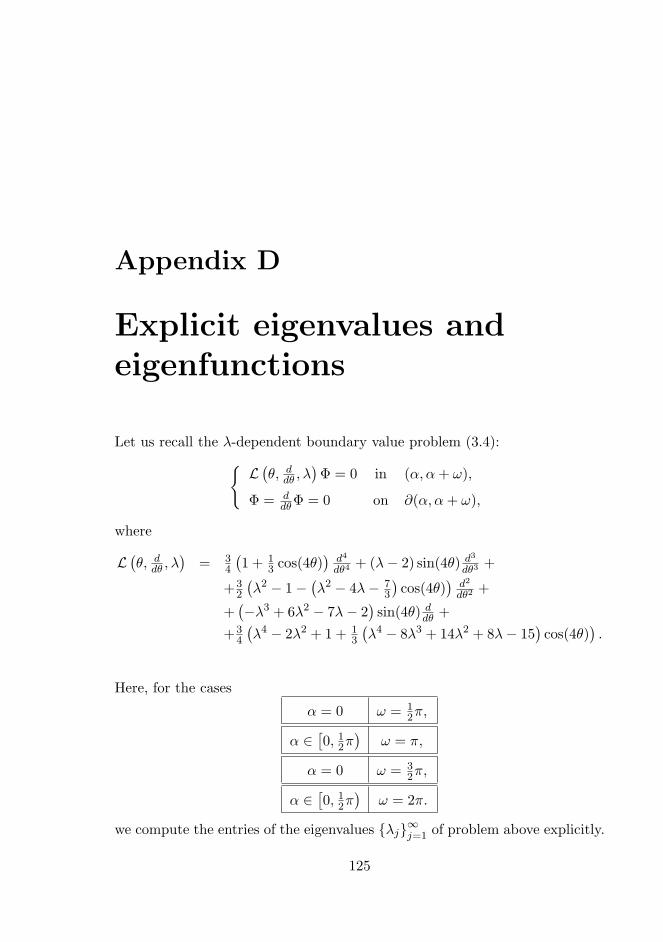
Appendix D
Explicit eigenvalues andeigenfunctions
Let us recall the λ-dependent boundary value problem (3.4):L(θ, ddθ , λ
)Φ = 0 in (α, α+ ω),
Φ = ddθΦ = 0 on ∂(α, α+ ω),
where
L(θ, ddθ , λ
)= 3
4
(1 + 1
3 cos(4θ))d4
dθ4+ (λ− 2) sin(4θ) d
3
dθ3+
+32
(λ2 − 1−
(λ2 − 4λ− 7
3
)cos(4θ)
)d2
dθ2+
+(−λ3 + 6λ2 − 7λ− 2
)sin(4θ) ddθ +
+34
(λ4 − 2λ2 + 1 + 1
3
(λ4 − 8λ3 + 14λ2 + 8λ− 15
)cos(4θ)
).
Here, for the cases
α = 0 ω = 12π,
α ∈[0, 1
2π)
ω = π,
α = 0 ω = 32π,
α ∈[0, 1
2π)
ω = 2π.
we compute the entries of the eigenvalues λj∞j=1 of problem above explicitly.
125

126APPENDIX D. EXPLICIT EIGENVALUES AND EIGENFUNCTIONS
Moreover, it will be possible to give the explicit formulas for the power-type solutions uj,q = rλj+1Φj,q, q = 0, ..., κj−1, to homogeneous problem (3.1)in the K(α,ω), namely,
uxxxx + uyyyy = 0 in K(α,ω),
u = 0 on ∂K(α,ω),
∂∂νu = 0 on ∂K(α,ω)\0.
We will do this in the following cases
α = 0 ω ∈
12π, π
for all λj ,
α = 0 ω ∈
32π, 2π
for some λj .
Remark D.1 When α ∈(0, 1
2π)
and ω = π one may easily compute the firstsolution u1,0 = r2 sin2(θ − α) to (3.1) in K(α,ω). The higher order solutionsuj,q will require more labor.
D.1 Computations for λj∞j=1
D.1.1 Case α = 0, ω = 12π
The eigenvalues λ in more general case, namely, α ∈[0, 1
2π)
and ω = 12π are
determined by the characteristic equation:(1−
√2
2 sin(2α))2λ
+(1 +
√2
2 sin(2α))2λ
+ 2(
12 + 1
2 cos2(2α))λ cos (λπ) +
−4(
12 + 1
2 cos2(2α))λ cos
λ[arctan
(tan2(α)
)− arctan
(cot2(α)
)]= 0,
where λ /∈ 0,±1. The left-hand side is obtained from formula (3.8).In particular case α = 0, we get
2 + 2 cos(πλ)− 4 cos(
12πλ
)= 0, λ /∈ 0,±1 ,
and the set of positive solutions of the above equation reads as:
λj∞j=1 = λ3j−2, λ3j−1, λ3j∞j=1 = −1 + 4j, 4j, 1 + 4j∞j=1 .
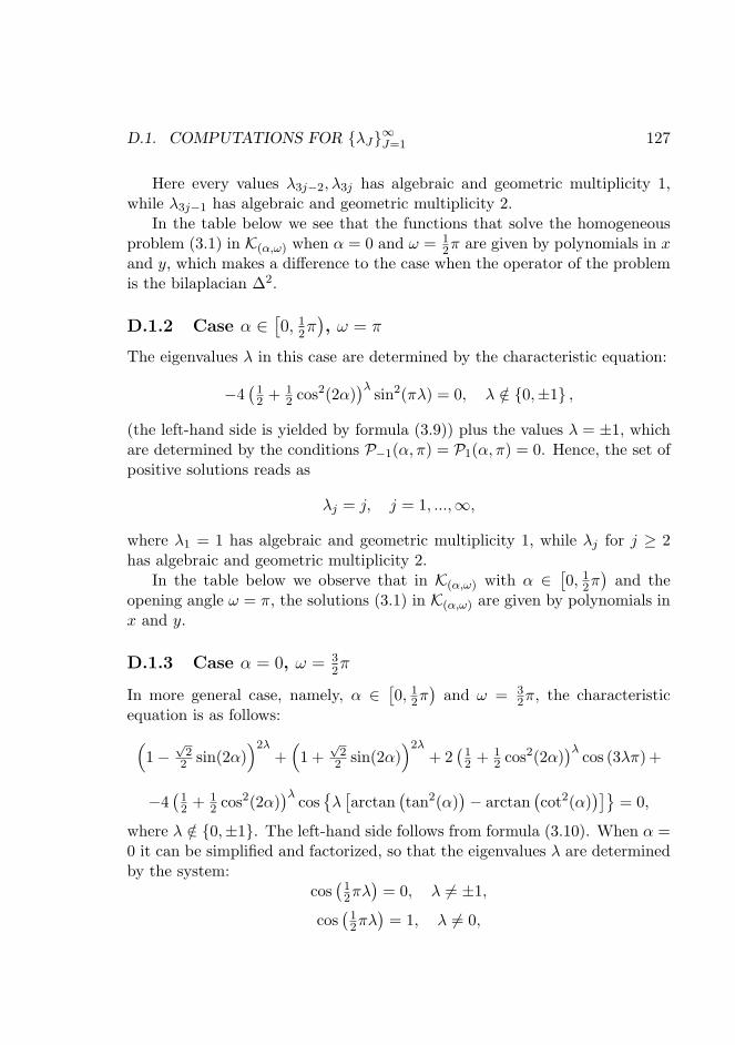
D.1. COMPUTATIONS FOR λJ∞J=1 127
Here every values λ3j−2, λ3j has algebraic and geometric multiplicity 1,while λ3j−1 has algebraic and geometric multiplicity 2.
In the table below we see that the functions that solve the homogeneousproblem (3.1) in K(α,ω) when α = 0 and ω = 1
2π are given by polynomials in xand y, which makes a difference to the case when the operator of the problemis the bilaplacian ∆2.
D.1.2 Case α ∈[0, 1
2π), ω = π
The eigenvalues λ in this case are determined by the characteristic equation:
−4(
12 + 1
2 cos2(2α))λ sin2(πλ) = 0, λ /∈ 0,±1 ,
(the left-hand side is yielded by formula (3.9)) plus the values λ = ±1, whichare determined by the conditions P−1(α, π) = P1(α, π) = 0. Hence, the set ofpositive solutions reads as
λj = j, j = 1, ...,∞,
where λ1 = 1 has algebraic and geometric multiplicity 1, while λj for j ≥ 2has algebraic and geometric multiplicity 2.
In the table below we observe that in K(α,ω) with α ∈[0, 1
2π)
and theopening angle ω = π, the solutions (3.1) in K(α,ω) are given by polynomials inx and y.
D.1.3 Case α = 0, ω = 32π
In more general case, namely, α ∈[0, 1
2π)
and ω = 32π, the characteristic
equation is as follows:(1−
√2
2 sin(2α))2λ
+(1 +
√2
2 sin(2α))2λ
+ 2(
12 + 1
2 cos2(2α))λ cos (3λπ) +
−4(
12 + 1
2 cos2(2α))λ cos
λ[arctan
(tan2(α)
)− arctan
(cot2(α)
)]= 0,
where λ /∈ 0,±1. The left-hand side follows from formula (3.10). When α =0 it can be simplified and factorized, so that the eigenvalues λ are determinedby the system:
cos(
12πλ
)= 0, λ 6= ±1,
cos(
12πλ
)= 1, λ 6= 0,
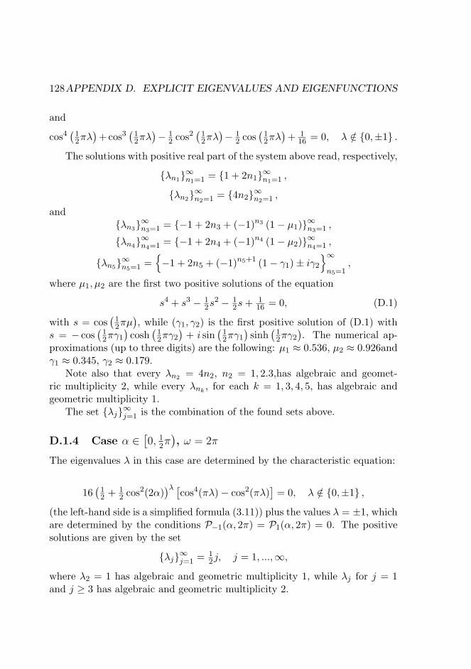
128APPENDIX D. EXPLICIT EIGENVALUES AND EIGENFUNCTIONS
and
cos4(
12πλ
)+cos3
(12πλ
)− 1
2 cos2(
12πλ
)− 1
2 cos(
12πλ
)+ 1
16 = 0, λ /∈ 0,±1 .
The solutions with positive real part of the system above read, respectively,
λn1∞n1=1 = 1 + 2n1∞n1=1 ,
λn2∞n2=1 = 4n2∞n2=1 ,
andλn3
∞n3=1 = −1 + 2n3 + (−1)n3 (1− µ1)∞n3=1 ,
λn4∞n4=1 = −1 + 2n4 + (−1)n4 (1− µ2)∞n4=1 ,
λn5∞n5=1 =
−1 + 2n5 + (−1)n5+1 (1− γ1)± iγ2
∞n5=1
,
where µ1, µ2 are the first two positive solutions of the equation
s4 + s3 − 12s
2 − 12s+ 1
16 = 0, (D.1)
with s = cos(
12πµ
), while (γ1, γ2) is the first positive solution of (D.1) with
s = − cos(
12πγ1
)cosh
(12πγ2
)+ i sin
(12πγ1
)sinh
(12πγ2
). The numerical ap-
proximations (up to three digits) are the following: µ1 ≈ 0.536, µ2 ≈ 0.926andγ1 ≈ 0.345, γ2 ≈ 0.179.
Note also that every λn2 = 4n2, n2 = 1, 2.3,has algebraic and geomet-ric multiplicity 2, while every λnk
, for each k = 1, 3, 4, 5, has algebraic andgeometric multiplicity 1.
The set λj∞j=1 is the combination of the found sets above.
D.1.4 Case α ∈[0, 1
2π), ω = 2π
The eigenvalues λ in this case are determined by the characteristic equation:
16(
12 + 1
2 cos2(2α))λ [cos4(πλ)− cos2(πλ)
]= 0, λ /∈ 0,±1 ,
(the left-hand side is a simplified formula (3.11)) plus the values λ = ±1, whichare determined by the conditions P−1(α, 2π) = P1(α, 2π) = 0. The positivesolutions are given by the set
λj∞j=1 = 12j, j = 1, ...,∞,
where λ2 = 1 has algebraic and geometric multiplicity 1, while λj for j = 1and j ≥ 3 has algebraic and geometric multiplicity 2.

D.2. THE LIST OF TABLES FOR UJ,Q 129
D.2 The list of tables for uj,q
j λj κj uj,q = rλj+1Φj,q(θ)
1 3 1 x2y2
2− 3 4 2
x3y2
x2y3
4 5 1 x3y3
5 7 1 x6y2 − x2y6
6− 7 8 2
x7y2 − 7
3x3y6
x2y7 − 73x
6y
8 9 1 x7y3 − x3y7
9 11 1 x10y2 − 14x6y6 + x2y10
10− 11 12 2
x11y2 − 22x7y6 + 11
3 x3y10
x2y11 − 22x6y7 + 113 x
10y3
12 13 1 x11y3 − 667 x
7y7 + x3y11
etc.
Table D.1: The first three groups of solutions solutions uj,q = rλj+1Φj,q(θ),q = 0, ..., κj − 1 to (3.1) in K(α,ω) when α = 0 and ω = 1
2π.
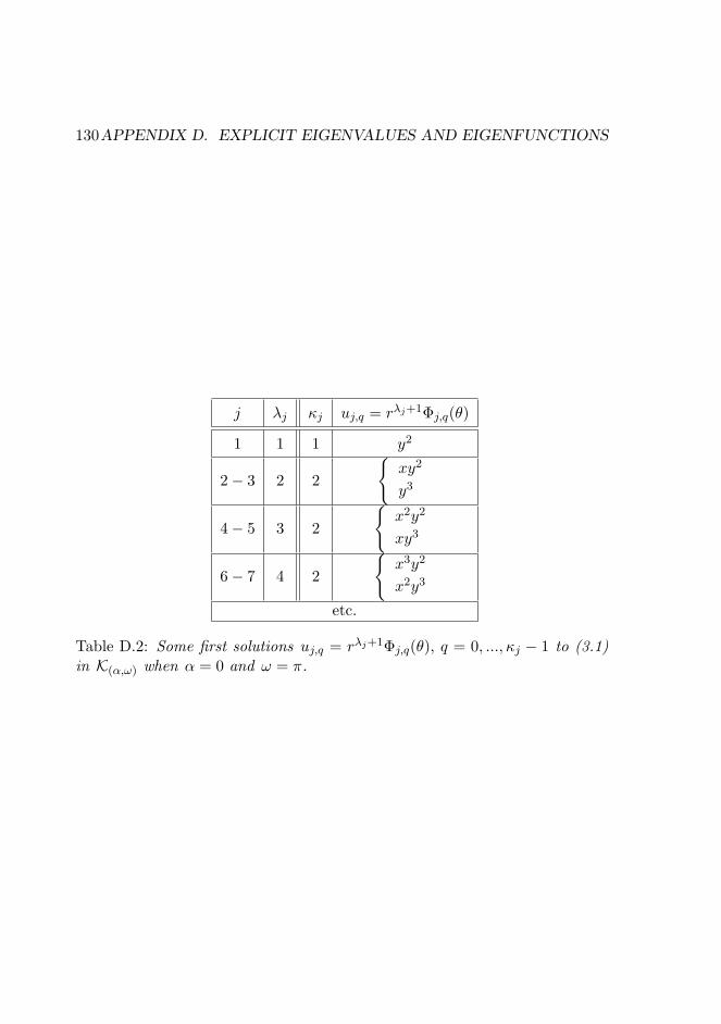
130APPENDIX D. EXPLICIT EIGENVALUES AND EIGENFUNCTIONS
j λj κj uj,q = rλj+1Φj,q(θ)
1 1 1 y2
2− 3 2 2
xy2
y3
4− 5 3 2
x2y2
xy3
6− 7 4 2
x3y2
x2y3
etc.
Table D.2: Some first solutions uj,q = rλj+1Φj,q(θ), q = 0, ..., κj − 1 to (3.1)in K(α,ω) when α = 0 and ω = π.
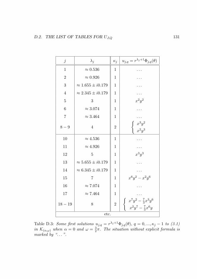
D.2. THE LIST OF TABLES FOR UJ,Q 131
j λj κj uj,q = rλj+1Φj,q(θ)
1 ≈ 0.536 1 . . .
2 ≈ 0.926 1 . . .
3 ≈ 1.655± i0.179 1 . . .
4 ≈ 2.345± i0.179 1 . . .
5 3 1 x2y2
6 ≈ 3.074 1 . . .
7 ≈ 3.464 1 . . .
8− 9 4 2
x3y2
x2y3
10 ≈ 4.536 1 . . .
11 ≈ 4.926 1 . . .
12 5 1 x3y3
13 ≈ 5.655± i0.179 1 . . .
14 ≈ 6.345± i0.179 1 . . .
15 7 1 x6y2 − x2y6
16 ≈ 7.074 1 . . .
17 ≈ 7.464 1 . . .
18− 19 8 2
x7y2 − 7
3x3y6
x2y7 − 73x
6y
etc.
Table D.3: Some first solutions uj,q = rλj+1Φj,q(θ), q = 0, ..., κj − 1 to (3.1)in K(α,ω) when α = 0 and ω = 3
2π. The situation without explicit formula ismarked by “. . . ”.
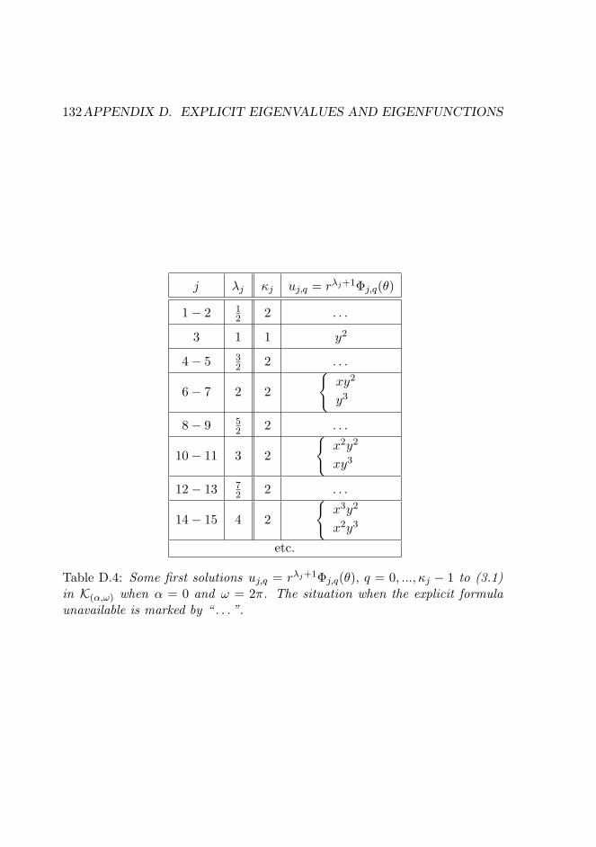
132APPENDIX D. EXPLICIT EIGENVALUES AND EIGENFUNCTIONS
j λj κj uj,q = rλj+1Φj,q(θ)
1− 2 12 2 . . .
3 1 1 y2
4− 5 32 2 . . .
6− 7 2 2
xy2
y3
8− 9 52 2 . . .
10− 11 3 2
x2y2
xy3
12− 13 72 2 . . .
14− 15 4 2
x3y2
x2y3
etc.
Table D.4: Some first solutions uj,q = rλj+1Φj,q(θ), q = 0, ..., κj − 1 to (3.1)in K(α,ω) when α = 0 and ω = 2π. The situation when the explicit formulaunavailable is marked by “ . . . ”.
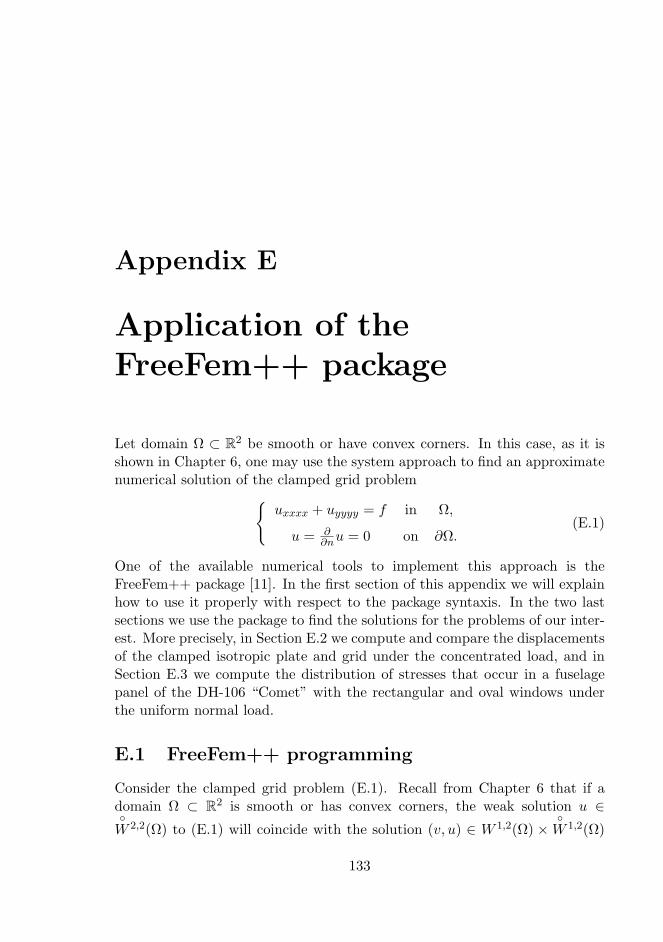
Appendix E
Application of theFreeFem++ package
Let domain Ω ⊂ R2 be smooth or have convex corners. In this case, as it isshown in Chapter 6, one may use the system approach to find an approximatenumerical solution of the clamped grid problem
uxxxx + uyyyy = f in Ω,
u = ∂∂nu = 0 on ∂Ω.
(E.1)
One of the available numerical tools to implement this approach is theFreeFem++ package [11]. In the first section of this appendix we will explainhow to use it properly with respect to the package syntaxis. In the two lastsections we use the package to find the solutions for the problems of our inter-est. More precisely, in Section E.2 we compute and compare the displacementsof the clamped isotropic plate and grid under the concentrated load, and inSection E.3 we compute the distribution of stresses that occur in a fuselagepanel of the DH-106 “Comet” with the rectangular and oval windows underthe uniform normal load.
E.1 FreeFem++ programming
Consider the clamped grid problem (E.1). Recall from Chapter 6 that if adomain Ω ⊂ R2 is smooth or has convex corners, the weak solution u ∈W 2,2(Ω) to (E.1) will coincide with the solution (v, u) ∈ W 1,2(Ω) ×
W 1,2(Ω)
133
134 APPENDIX E. APPLICATION OF THE FREEFEM++ PACKAGE
of the following variational problem∫Ω
[(∂v∂x +
√2
2∂v∂y
)∂ψ∂x +
(∂v∂y +
√2
2∂v∂x
)∂ψ∂y+
+(∂u∂x −
√2
2∂u∂y
)∂φ∂x +
(∂u∂y −
√2
2∂u∂x
)∂φ∂y − fψ − vφ
]dxdy = 0,
for all (φ, ψ) ∈W 1,2(Ω)×W 1,2(Ω). (E.2)
In this section we will bring the numerical evidence for this assertion athand. In order to do this we will choose such the right-hand side f in prob-lem (E.1) for which the explicit solution u is available. Then we will let theFreeFem++ package solve equation (E.2) for this given f and compare ob-tained u with the known original one. In this way one shows the feasibility ofthe system approach to problem (E.1). Also, some technical details on how torealize equation (E.2) in the FreeFem++ package will be discussed.
E.1.1 The test problem
Let us consider the functions ϕi : [0, 1] → R, i ∈ N given explicitly as
ϕi(x) =cosh(νix)− cos(νix)cosh(νi)− cos(νi)
− sinh(νix)− sin(νix)sinh(νi)− sin(νi)
, (E.3)
where νi is the ith positive solution of the transcendental equationcos(ν) cosh(ν) = 1.
Let Ω := [0, 1]2. One directly shows that the function
Φij(x, y) = ϕi(x)ϕj(y), i, j ∈ N, (E.4)
solves the problem(∂4
∂x4 + ∂4
∂y4
)Φij =
(ν4i + ν4
j
)Φij in Ω,
Φij = ∂∂nΦij = 0 on ∂Ω\S,
where S = (0, 0), (0, 1), (1, 0), (1, 1).Consider the test boundary value problem:
uxxxx + uyyyy = f := 2ν41Φ11 in Ω,
u = ∂∂nu = 0 on ∂Ω\S,
(E.5)
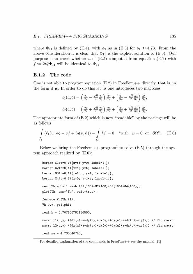
E.1. FREEFEM++ PROGRAMMING 135
where Φ11 is defined by (E.4), with φ1 as in (E.3) for ν1 ≈ 4.73. From theabove consideration it is clear that Φ11 is the explicit solution to (E.5). Ourpurpose is to check whether u of (E.5) computed from equation (E.2) withf := 2ν4
1Φ11 will be identical to Φ11.
E.1.2 The code
One is not able to program equation (E.2) in FreeFem++ directly, that is, inthe form it is. In order to do this let us one introduces two macroses
`1(a, b) =(∂a∂x −
√2
2∂a∂y
)∂b∂x +
(∂a∂y −
√2
2∂a∂x
)∂b∂y ,
`2(a, b) =(∂a∂x +
√2
2∂a∂y
)∂b∂x +
(∂a∂y +
√2
2∂a∂x
)∂b∂y .
The appropriate form of (E.2) which is now “readable” by the package will beas follows∫
Ω
(`1(w, φ)− vφ+ `2(v, ψ))−∫Ω
fψ = 0 “with w = 0 on ∂Ω”. (E.6)
Below we bring the FreeFem++ program1 to solve (E.5) through the sys-tem approach realized by (E.6):
border G1(t=0,1)x=t; y=0; label=1;;border G2(t=0,1)x=1; y=t; label=1;;border G3(t=0,1)x=1-t; y=1; label=1;;border G4(t=0,1)x=0; y=1-t; label=1;;
mesh Th = buildmesh (G1(100)+G2(100)+G3(100)+G4(100));
plot(Th, cmm="Th", wait=true);
fespace Vh(Th,P1);
Vh w,v, psi,phi;
real k = 0.707106781186550;
macro l1(u,v) ((dx(u)-a*dy(u))*dx(v)+(dy(u)-a*dx(u))*dy(v)) // fin macro
macro l2(u,v) ((dx(u)+a*dy(u))*dx(v)+(dy(u)+a*dx(u))*dy(v)) // fin macro
real nu = 4.730040745;
1For detailed explanation of the commands in FreeFem++ see the manual [11]
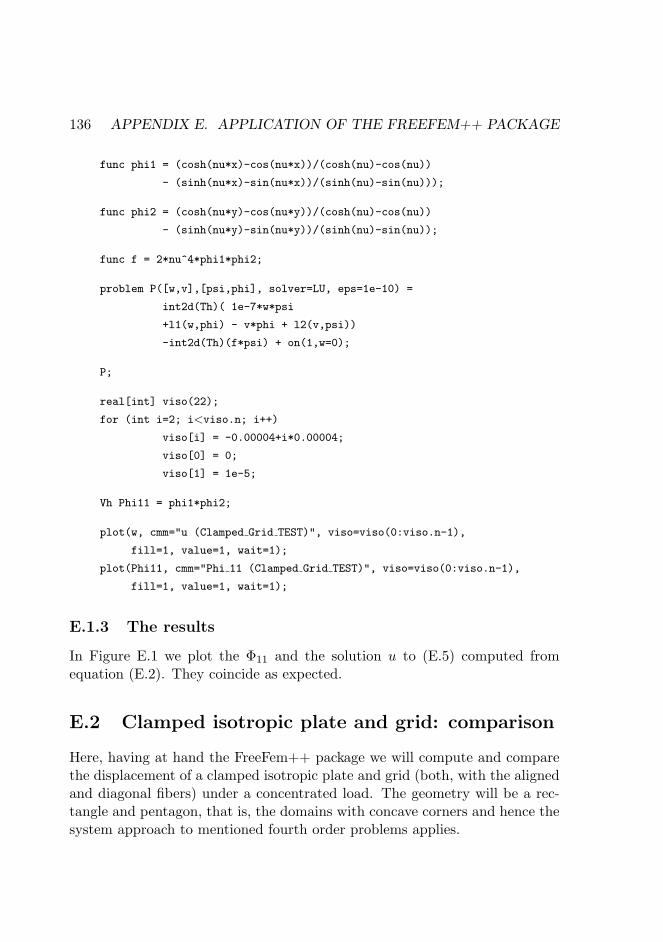
136 APPENDIX E. APPLICATION OF THE FREEFEM++ PACKAGE
func phi1 = (cosh(nu*x)-cos(nu*x))/(cosh(nu)-cos(nu))
- (sinh(nu*x)-sin(nu*x))/(sinh(nu)-sin(nu)));
func phi2 = (cosh(nu*y)-cos(nu*y))/(cosh(nu)-cos(nu))
- (sinh(nu*y)-sin(nu*y))/(sinh(nu)-sin(nu));
func f = 2*nu^4*phi1*phi2;
problem P([w,v],[psi,phi], solver=LU, eps=1e-10) =
int2d(Th)( 1e-7*w*psi
+l1(w,phi) - v*phi + l2(v,psi))
-int2d(Th)(f*psi) + on(1,w=0);
P;
real[int] viso(22);
for (int i=2; i<viso.n; i++)
viso[i] = -0.00004+i*0.00004;
viso[0] = 0;
viso[1] = 1e-5;
Vh Phi11 = phi1*phi2;
plot(w, cmm="u (Clamped Grid TEST)", viso=viso(0:viso.n-1),
fill=1, value=1, wait=1);
plot(Phi11, cmm="Phi 11 (Clamped Grid TEST)", viso=viso(0:viso.n-1),
fill=1, value=1, wait=1);
E.1.3 The results
In Figure E.1 we plot the Φ11 and the solution u to (E.5) computed fromequation (E.2). They coincide as expected.
E.2 Clamped isotropic plate and grid: comparison
Here, having at hand the FreeFem++ package we will compute and comparethe displacement of a clamped isotropic plate and grid (both, with the alignedand diagonal fibers) under a concentrated load. The geometry will be a rec-tangle and pentagon, that is, the domains with concave corners and hence thesystem approach to mentioned fourth order problems applies.
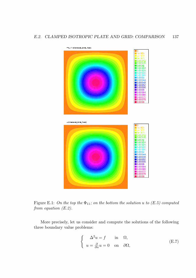
E.2. CLAMPED ISOTROPIC PLATE AND GRID: COMPARISON 137
Figure E.1: On the top the Φ11; on the bottom the solution u to (E.5) computedfrom equation (E.2).
More precisely, let us consider and compute the solutions of the followingthree boundary value problems:
∆2u = f in Ω,
u = ∂∂nu = 0 on ∂Ω,
(E.7)
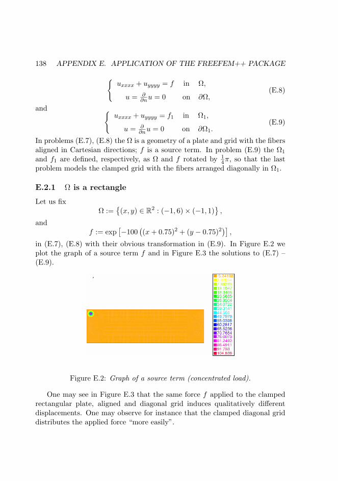
138 APPENDIX E. APPLICATION OF THE FREEFEM++ PACKAGE
uxxxx + uyyyy = f in Ω,
u = ∂∂nu = 0 on ∂Ω,
(E.8)
and uxxxx + uyyyy = f1 in Ω1,
u = ∂∂nu = 0 on ∂Ω1.
(E.9)
In problems (E.7), (E.8) the Ω is a geometry of a plate and grid with the fibersaligned in Cartesian directions; f is a source term. In problem (E.9) the Ω1
and f1 are defined, respectively, as Ω and f rotated by 14π, so that the last
problem models the clamped grid with the fibers arranged diagonally in Ω1.
E.2.1 Ω is a rectangle
Let us fixΩ :=
(x, y) ∈ R2 : (−1, 6)× (−1, 1)
,
andf := exp
[−100
((x+ 0.75)2 + (y − 0.75)2
)],
in (E.7), (E.8) with their obvious transformation in (E.9). In Figure E.2 weplot the graph of a source term f and in Figure E.3 the solutions to (E.7) –(E.9).
Figure E.2: Graph of a source term (concentrated load).
One may see in Figure E.3 that the same force f applied to the clampedrectangular plate, aligned and diagonal grid induces qualitatively differentdisplacements. One may observe for instance that the clamped diagonal griddistributes the applied force “more easily”.

E.2. CLAMPED ISOTROPIC PLATE AND GRID: COMPARISON 139
Figure E.3: Displacement of, respectively, an isotropic rectangular plate, gridwith the aligned fibers and grid with the diagonal fibers, under a concentratedload depicted in Figure E.2.
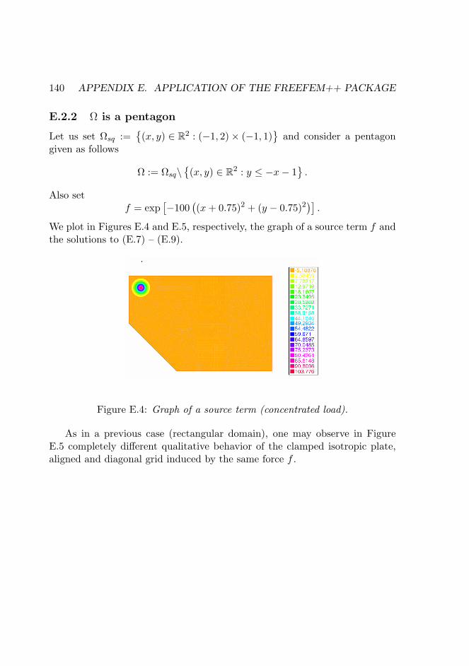
140 APPENDIX E. APPLICATION OF THE FREEFEM++ PACKAGE
E.2.2 Ω is a pentagon
Let us set Ωsq :=(x, y) ∈ R2 : (−1, 2)× (−1, 1)
and consider a pentagon
given as follows
Ω := Ωsq\(x, y) ∈ R2 : y ≤ −x− 1
.
Also setf = exp
[−100
((x+ 0.75)2 + (y − 0.75)2
)].
We plot in Figures E.4 and E.5, respectively, the graph of a source term f andthe solutions to (E.7) – (E.9).
Figure E.4: Graph of a source term (concentrated load).
As in a previous case (rectangular domain), one may observe in FigureE.5 completely different qualitative behavior of the clamped isotropic plate,aligned and diagonal grid induced by the same force f .

E.2. CLAMPED ISOTROPIC PLATE AND GRID: COMPARISON 141
Figure E.5: Displacement of, respectively, an isotropic rectangular plate, gridwith the aligned fibers and grid with the diagonal fibers, under a concentratedload depicted in Figure E.4.
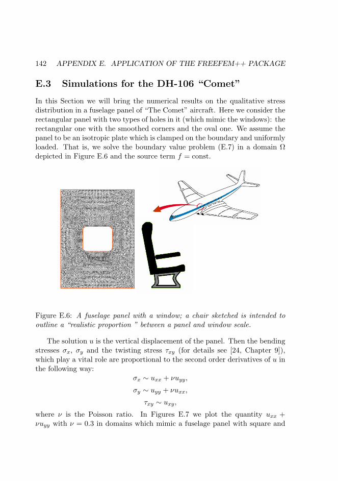
142 APPENDIX E. APPLICATION OF THE FREEFEM++ PACKAGE
E.3 Simulations for the DH-106 “Comet”
In this Section we will bring the numerical results on the qualitative stressdistribution in a fuselage panel of “The Comet” aircraft. Here we consider therectangular panel with two types of holes in it (which mimic the windows): therectangular one with the smoothed corners and the oval one. We assume thepanel to be an isotropic plate which is clamped on the boundary and uniformlyloaded. That is, we solve the boundary value problem (E.7) in a domain Ωdepicted in Figure E.6 and the source term f = const.
Figure E.6: A fuselage panel with a window; a chair sketched is intended tooutline a “realistic proportion ” between a panel and window scale.
The solution u is the vertical displacement of the panel. Then the bendingstresses σx, σy and the twisting stress τxy (for details see [24, Chapter 9]),which play a vital role are proportional to the second order derivatives of u inthe following way:
σx ∼ uxx + νuyy,
σy ∼ uyy + νuxx,
τxy ∼ uxy,
where ν is the Poisson ratio. In Figures E.7 we plot the quantity uxx +νuyy with ν = 0.3 in domains which mimic a fuselage panel with square and
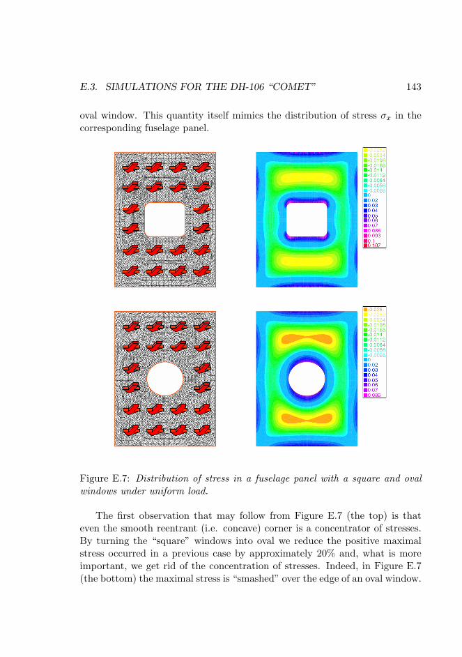
E.3. SIMULATIONS FOR THE DH-106 “COMET” 143
oval window. This quantity itself mimics the distribution of stress σx in thecorresponding fuselage panel.
Figure E.7: Distribution of stress in a fuselage panel with a square and ovalwindows under uniform load.
The first observation that may follow from Figure E.7 (the top) is thateven the smooth reentrant (i.e. concave) corner is a concentrator of stresses.By turning the “square” windows into oval we reduce the positive maximalstress occurred in a previous case by approximately 20% and, what is moreimportant, we get rid of the concentration of stresses. Indeed, in Figure E.7(the bottom) the maximal stress is “smashed” over the edge of an oval window.
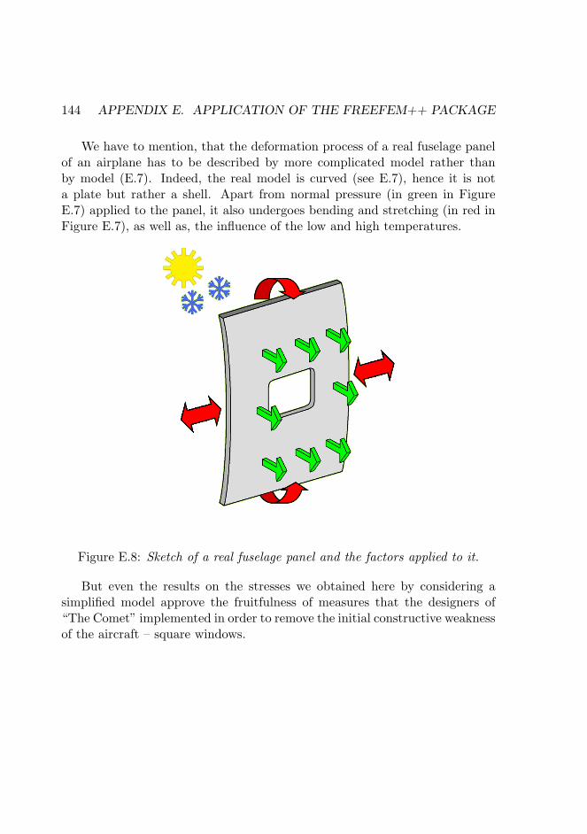
144 APPENDIX E. APPLICATION OF THE FREEFEM++ PACKAGE
We have to mention, that the deformation process of a real fuselage panelof an airplane has to be described by more complicated model rather thanby model (E.7). Indeed, the real model is curved (see E.7), hence it is nota plate but rather a shell. Apart from normal pressure (in green in FigureE.7) applied to the panel, it also undergoes bending and stretching (in red inFigure E.7), as well as, the influence of the low and high temperatures.
Figure E.8: Sketch of a real fuselage panel and the factors applied to it.
But even the results on the stresses we obtained here by considering asimplified model approve the fruitfulness of measures that the designers of“The Comet” implemented in order to remove the initial constructive weaknessof the aircraft – square windows.
Bibliography
[1] Bernoulli, Jacob II., Essai theoretique sur les vibrations des plaqueselastiques, rectangulaires et libres. Nova Acta Academiae Scientiarum Im-perialis Petropolitanae V (1789), p.197.
[2] C. Bandle, M. Flucher, Table of inequalities in elliptic boundary valueproblems, Recent progress in inequalities, Series: Math. Appl., vol. 430(1996), pp. 97–125.
[3] H. Blum, R. Rannacher, On the boundary value problem of the biharmonicoperator on domains with angular corners, Math. Meth. in the Appl. Sci.2 (1980), pp. 556–581.
[4] M. Costabel, M. Dauge, S. Nicaise, editors. Boundary value problems andintegral equations in nonsmooth domains, Lecture Notes in Ppure andApllied Mathematics, Vol. 167. Marcel Dekker, Inc., New York, 1995.
[5] Ph. Clement, G. Sweers, Uniform anti-maximum principles, J.DifferentialEquations 164 (2000), pp. 118–154.
[6] B. Dacorogna, Introduction to the calculus of variations, Imperial CollegePress, London, 2004.
[7] M. Dauge, Elliptic boundary value problems on corner domains; smooth-ness and asymptotics of solutions, Springer, Berlin, 1988.
[8] C. Davini, Γ-convergence of External Approximations in Boundary ValueProblems Involving the bi-Laplacian, Journal of Computational and Ap-plied Mathematics, Vol. 140 (2002), pp. 185–208.
[9] P. Drabek, J. Milota, Methods of Nonlinear Analysis: Applications toDifferential Equations, Birkhauser Verlag, Basel, 2007.
145
146 BIBLIOGRAPHY
[10] L.C. Evans, Partial differential equations. Graduate Studies in Mathe-matics, 19. American Mathematical Society, Providence, RI, 1998.
[11] FreeFem++, http://www.freefem.org/ff++/
[12] T. Gerasimov, G. Sweers, The regularity for a clamped grid equa-tion uxxxx + uyyyy = f in a domain with corner, Electronic Jour-nal of Differential Equations, vol. 2009 (2009), No. 47, pp. 1–54.http://ejde.math.txstate.edu/
[13] T. Gerasimov, A. Stylianou, G. Sweers, A failure in the Hamiltonianapproach to the clamped plate equation, submitted.
[14] P. Grisvard, Singularities in boundary value problems, Springer-Verlag,Berlin, 1992.
[15] http://www.geocities.com/CapeCanaveral/Lab/8803/comet.htm
[16] http://aviation-safety.net/database/record.php?id=19540110-1
[17] G. Kirchhoff, Uber das Gleichgewicht und die Bewegung einer elastischenScheibe, J. Reine Angew. Math. 40 (1850), pp. 51–88.
[18] V.A. Kondratiev, Boundary value problems for elliptic equations in do-mains with conical or angular points, Trudy Moskov. Mat. Obsc. 16(1967), pp. 209–292 (in Russian), English transl.: Trans. Moscow Math.Soc. 16 (1967), pp. 227–313.
[19] V.A. Kozlov, V.G. Maz’ya, J. Rossmann, Elliptic Boundary Value Prob-lems in Domains with Point Singularities, Mathematical Surveys andMonographs, vol. 52, American Mathematical Society, Providence, RI,1997.
[20] V.A. Kozlov, V.G. Maz’ya, J. Rossmann, Spectral problems associatedwith corner singularities of solutions to elliptic equations, MathematicalSurveys and Monographs, vol. 85, American Mathematical Society, Prov-idence, RI, 2001.
[21] B. Kawohl, G. Sweers, On the differential equation uxxxx + uyyyy = f foran anisotropic stiff material, SIAM J. Math. Anal., Vol. 37, No. 6 (2006),pp. 1828–1853.
BIBLIOGRAPHY 147
[22] O.A. Ladyzhenskaya, N.N. Ural’tseva, Linear and quasilinear ellipticequations, Academic Press, NY, 1968.
[23] D. Leguillon, E. Sanchez-Palencia, Computation of singular solutions inelliptic problems and elasticity, Masson, Paris, 1987.
[24] S.G. Lekhnitskii, Anisotropic plates, 2nd edition, translated from Russian,Gordon and Breach, New York, 1968.
[25] J.-L. Lions, E. Magenes, Non-homogeneous boundary value problems andapplications, Vol. I, Springer-Verlag, Berlin, 1972.
[26] S.A. Nazarov, B.A. Plamenevsky, Elliptic problems in domains with piece-wise smooth boundaries, De Gruyter, Berlin, 1994.
[27] S.A. Nazarov, A. Slutskij, G. Sweers, Korn’s inequalities for a reinforcedplate, submitted.
[28] S.A. Nazarov, G. Sweers, A hinged plate equation and iterated DirichletLaplace operator on domains with concave corners, J. Differential Equa-tions 233 (2007), pp. 151–180.
[29] R.S. Palais, The Morse lemma for Banach spaces, Bull. Amer. Math. Soc.75 (1969), pp. 968–971.
[30] M.L. Williams, Surface Stress Singularities Resulting From VariousBoundary Conditions in Angular Corners of Plates Under Bending, Pro-ceedings of the First U.S. National Congress of Applied Mechanics, IllinoisInstitute of Technology, Chicago, 1951, pp. 325–329.

Summary
The main focus of this thesis is the regularity question for the fourth orderelliptic problem
uxxxx + uyyyy = f in Ω,
u = ∂∂nu = 0 on ∂Ω,
(S.1)
in an open and bounded domain Ω ⊂ R2 which has one corner in 0 ∈ ∂Ω withopening angle ω ∈ (0, 2π]. Here n stands for the outward normal on ∂Ω.
For the right-hand side f ∈ L2(Ω) problem (S.1) has a unique weak solu-
tion u ∈W 2,2(Ω) (see Chapter 2). We study the optimal regularity2 of this
weak solution and more specifically near a corner of the domain. Within theframework of the Kondratiev theory developed to treat the problems of type(S.1) in domains with corner singularities, it holds that for f ∈ L2(Ω) the
weak solution u ∈W 2,2(Ω) to (S.1) possesses the asymptotic representation:
u = w +∑
0<Re(λj)<2
κj−1∑q=0
cj,qrλj+1(log(r))qΦj,q (λj , θ) , (S.2)
where w ∈ W 4,2(Ω) and the double sum are, respectively, a regular and aso-called “singular” parts of u. The singular part written down in the polarcoordinates (r, θ) represents the behavior of the solution u locally in the vicin-ity of an angular point 0. In formula (S.2), cj,q are the constants, λj are thesolutions of a certain transcendental equation, κj is the algebraic multiplicityof each λj , the functions Φj,q are infinitely differentiable.
2In a classical sense, that is, under appropriate smoothness assumptions for ∂Ω, theoptimal regularity for the solution means: if f ∈ W k,p(Ω), then u ∈ W k+4,p(Ω), where k ≥ 0and p ∈ (1,∞). Due to the presence of a corner, this result for problem (S.1) in general doesnot apply.
149

150 SUMMARY
The key parameters in (S.2) are the exponents λj , particularly, the λ1 asit defines the differentiability of the whole singular part of u. For the presentoperator L = ∂4
∂x4 + ∂4
∂y4in (S.1) it holds that
(0, 2π]×[0, 1
2π)3 (ω, α) 7→ Re(λ1(ω, α)),
that is, λ1 is a function of the opening angle ω and the parameter α. Thelatter defines orientation of a domain Ω in a coordinate system (x, y).
A striking consequence of the precise regularity described in this thesis isthe existence of at least one interval
(12π, ω?
), ω?/π ≈ 0.528 (in degrees ω? ≈
95.1), on which λ1 is the increasing function of ω. In terms of the optimalregularity this result means that the differential properties of solution u to(S.1) improve with increasing opening angle, what makes a drastic differenceto the Laplacian and bilaplacian models. The rigorous proof concerns the caseα = 0 (Chapter 3) and for α ∈
(0, 1
2π)
we only give the numerical results forthe behavior of λ1 on the interval ω ∈ (0, 2π]. The regularity statement forthe solution u to (S.1) in terms of the weighted and standard Sobolev spacesis given in Chapter 5. It implements the embedding results for the spaces inquestion which is elaborated in the foregoing Chapter 4.
A secondary result of the research presented addresses the possibility tosolve the fourth order problem (S.1) in a domain Ω with the opening angleω ∈ (0, 2π] through the system approach:
−∆v −√
2vxy = f in Ω,
−∆u+√
2uxy = v in Ω,
u = ∂∂nu = 0 on ∂Ω.
(S.5)
Thus, in Chapter 6 we show that for every α ∈ [0, 12π) the corresponding weak
solutions u ∈W 2,2(Ω) to (S.1) and (v, u) ∈ W 1,2(Ω) ×
W 1,2(Ω) to problem
(S.5) will coincide if the opening angle ω satisfies ω ≤ π. In general, this isnot the case for all ω > π.
Appendix A contains a result, which is although not related directly toproblem (S.1) yet may be of interesting in the applications. Here we provethat for every fourth order elliptic operator
L = ∂4
∂x4 + b1∂4
∂x3∂y+ b2
∂4
∂x2∂y2+ b3
∂4
∂x∂y3+ ∂4
∂y4, (S.3)

SUMMARY 151
with bj ∈ R, j = 1, 2, 3, there exists precisely one a ∈ [1,+∞) such that L isalgebraically equivalent to the operator
La = ∂4
∂x4 + 2a ∂4
∂x2∂y2+ ∂4
∂y4. (S.4)
That is, one may always find an appropriate linear coordinate transforma-tion such that due to this transformation the operator L turns into La witha ∈ [1,+∞). This result is based on the Mobius mapping. In the mechan-ical context this transformation result for the operator L means that therealways exists a coordinate system such that in this system every anisotropic2d-medium is viewed as an orthotropic one.
Appendices B–D contain all supplementary computational and numericalresults, while in Appendix E we use the approach developed in the last chapterof the thesis for the numerical treatment of some applied problems.

Samenvatting
Het ingeklemde elastische rooster,
een vierde orde vergelijking
op een gebied met hoek
van Tymofiy Gerasimov
Het centrale thema van dit proefschrift is de regulariteitsvraag voor hetvierde orde elliptische probleem
uxxxx + uyyyy = f in Ω,
u = ∂∂nu = 0 on ∂Ω,
(S.1)
in een open en begrensd gebied Ω ⊂ R2, dat een hoek bevat in 0 ∈ ∂Ωmet als opening ω ∈ (0, 2π]. De letter n staat voor de naar buiten gerichtenormaalvektor op ∂Ω.
Voor de rechterzijde f ∈ L2(Ω) heeft probleem (S.1) een eenduidige zwakke
oplossing u ∈W 2,2(Ω) (zie Hoofdstuk 2). We onderzoeken de optimale regu-
lariteit3 van deze zwakke oplossing in het bijzonder bij de hoek van dit gebied.Volgens de door Kondratiev ontwikkelde theorie voor problemen van het type(S.1), heeft de zwakke oplossing voor f ∈ L2(Ω) de volgende asymptotischeontwikkeling:
3In de klassieke zin, onder voldoende gladheid van de rand ∂Ω, geldt voor de optimaleregulariteit: als f ∈ W k,p(Ω), dan geldt u ∈ W k+4,p(Ω), voor k ≥ 0 en p ∈ (1,∞). Door deaanwezigheid van een hoek, is dit resultaat voor (S.1) in het algemeen niet van toepassing.
153
154 SAMENVATTING
u = w +∑
0<Re(λj)<2
κj−1∑q=0
cj,qrλj+1(log(r))qΦj,q (λj , θ) , (S.2)
waarbij w ∈ W 4,2(Ω) en de dubbele som respectievelijk het reguliere en het“singular” deel van de oplossing u vormen. Het singuliere deel is in poolco-ordinaten (r, θ) beschreven en vertegenwoordigd het gedrag van de oplossingu bij het hoekpunt. In formule (S.2), zijn cj,q konstanten, zijn λj oplossingenvan een bepaalde transcendentale vergelijking, zijn de κj de algebraısche mul-tipliciteiten van λj en vormen de Φj,q oplossingen van een bepaalde gewone dif-ferentiaalvergelijking met bijbehorende randwaarden. Deze Φj,q zijn oneindigvaak differentieerbaar.
De cruciale parameters in (S.2) zijn de λj , in het bijzonder λ1 omdatdeze de differentierbaarheid van het singuliere deel bepaalt. Voor de huidigeoperator L = ∂4
∂x4 + ∂4
∂y4in (S.1) geldt dat
(0, 2π]×[0, 1
2π)3 (ω, α) 7→ Re(λ1(ω, α)),
dat wil zeggen, λ1 is een functie van de openingshoek ω en de parameterα. De laatste definiert de orientatie van het gebied Ω ten opzichte van hetcoordinatensysteem (x, y).
Een opvallend gevolg van het regulariteitsresultaat in dit proefschrift isde existentie van minstens een interval
(12π, ω?
), ω?/π ≈ 0.528 (in graden
ω? ≈ 95.1), waar λ1 een stijgende functie van ω is. Voor de optimale regular-iteit betekent dit, dat de differentieerbaarheidseigenschappen van de oploss-ing u van (S.1) verbeteren bij toenemende hoek en dit is tegengesteld aanhet gedrag bij randwaardeproblemen met de laplace- en bilaplace-operatoren.Een rigoreus bewijs betreft het geval α = 0 (Hoofdstuk 3); voor α ∈
(0, 1
2π)
geven we alleen de numerieke resultaten voor λ1 op het interval ω ∈ (0, 2π].Het regulariteitsresultaat voor de oplossing u van (S.1) in de zin van gewogenen standaard Sobolev-ruimten vindt men in Hoofdstuk 5. Het gebruikt deimbeddingsresultaten die uitgewerkt zijn in het voorafgaande Hoofdstuk 4.
Een secundair resultaat van het gepresenteerde onderzoek betreft de demogelijkheid om het vierde orde probleem (S.1) in een gebied Ω door middel
SAMENVATTING 155
van een systeem op te lossen:−∆v −
√2vxy = f in Ω,
−∆u+√
2uxy = v in Ω,
u = ∂∂nu = 0 on ∂Ω.
(S.5)
In Hoofdstuk 6 bewijzen we namelijk dat voor iedere α ∈ [0, 12π) de bijbe-
horende zwakke oplossing u ∈W 2,2(Ω) van (S.1) en (v, u) ∈W 1,2(Ω)×
W 1,2(Ω)
van probleem (S.5) overeenkomen wanneer de openingshoek ω kleiner als π is.In het algemeen is dit niet het geval voor ω > π.
Appendix A bevat een resultaat, dat ofschoon niet direct verwant metprobleem (S.1) niettemin interessant kan zijn voor de toepassingen. Daarbewijzen we dat er voor iedere vierde orde elliptische operator
L = ∂4
∂x4 + b1∂4
∂x3∂y+ b2
∂4
∂x2∂y2+ b3
∂4
∂x∂y3+ ∂4
∂y4, (S.3)
met bj ∈ R, j = 1, 2, 3, er precies een a ∈ [1,+∞) bestaat zodanig, dat Lalgebraısch equivalent is met de operator
La = ∂4
∂x4 + 2a ∂4
∂x2∂y2+ ∂4
∂y4. (S.4)
In andere woorden, er bestaat een lineaire coordinatentransformatie zodatL in La verandert in dit nieuwe stelsel. Dit resultaat is gebaseerd op eengeschikt gekozen Mobius-afbeelding. In de mechanische kontext betekent het,dat men altijd een coordinatensysteem zodaning kiezen kan dat het anisotrope2d-medium als een orthotroop medium beschouwd kan worden.
Appendices B–D bevatten alle supplementaire rekentechnische en numeriekeresultaten, terwijl in Appendix E de aanpak van het laatste hoofdstuk ont-wikkeld wordt voor de numerieke behandeling van enkele toegepaste proble-men.


Acknowledgement
At the end of this thesis I would like to thank all the people who contributeddirectly and indirectly in this result of mine.
First of all I would like to thank Guido Sweers, my scientific supervisor,who introduced me to this research area. I am grateful for his openness in dis-cussions, guidance and constant willingness to explain the abstract yet some-times obvious and simple mathematical tricks I am supposed to know, but havenever heard before. I benefited a lot from his expertise on the subject, supportand encouragement: I expanded my mathematical outlook, gained courage totackle potentially tricky problems and also learned how to formulate thoughtsin a precise and consistent manner.
All the other PhD-students of the Functional Analysis Group who havebeen my office-fellows during these four years, contributed to the nice workingatmosphere: Anna Dall’Acqua, Jan Maas, Mark Veraar, Mahmoud Barounand Sonja Cox. I am indebted to Sonja for improving my English and, espe-cially, for her help with the translation of the Propositions into Dutch. Also,my words of gratitude go to the secretary of the Analysis Group Dori Steenekenand the computer expert Xiwei Wu for their openness and constant willingnessto help.
I would like to thank Prof. dr. Victor Gristchak, the first scientific supervi-sor of mine in Ukraine, for introducing me to the world of science (perturbationmethods and hybrid techniques). It’s got obvious for me now that he “keptpushing” me in the right direction even when I did not realize that.
I am greatly indebted to Prof. dr. Igor Andrianov for his informal friendlyattitude and attention he paid to my humble person in a moment when I feltconfused about my scientific prospectives. He was the one who encouragedme to do PhD abroad and has been keeping his interest in the progress of mywork.
Also, I would like to express my gratitude to Dr. ir. Wim van Horssen for
157

158 ACKNOWLEDGEMENT
the possibility to come to Delft and for his open and considerate manner todiscuss and resolve the administrative questions.
A big thanks goes to the CICAT ladies Theda Olsder and Veronique van derVarst, for their assistance in handling many vitally important administrativematters that a foreign PhD-student may encounter in the Netherlands.
I would like to acknowledge the friends of mine in Delft, Alexey Andrianovand Alexander Pischanskiy, for a nice spirit of our conversation and help.
Finally, I thank my whole family for their love, encouragement and support.
Delft, September 2009 Tymofiy Gerasimov

Curriculum Vitae
Tymofiy Gerasimov was born in July 27, 1977 inTajikistan, one of the republics of the former SovietUnion.
In 1994 he completed his high school education atthe gymnasium N28 in Zaporizhzhia, Ukraine andpursued the study of Applied Mathematics at theZaporizhzhia State University (since 2005, the Za-porizhzhia National University).
After graduation, between 1999 and 2004, he wasinvolved in the teaching and research activity at theApplied Mathematics Department and the Solid Mechanics Group of the sameuniversity.
In January 2005 he started his PhD research at the Functional Analysis Groupat the Delft University of Technology under the supervision of Prof. dr. G.H.Sweers.
159