the cognitive cost of daycare 0{2 for children in...
TRANSCRIPT

The cognitive cost of daycare 0–2 for children in advantaged families∗
Margherita Fort§ Andrea Ichino¶ Giulio Zanella§
February 8, 2017
Abstract
Exploiting admission thresholds to the highly-reputed daycare system of Bologna, Italy,we show in a RDD that one additional month in daycare at age 0–2 reduces IQ by0.5% (4.5% of a s.d.) at age 8–14 in a relatively affluent population. This findingis consistent with the hypothesis, suggested in psychology, that children in daycareexperience fewer one-to-one interactions with adults, with negative effects in familieswhere such interactions are of particularly high quality. We show in a model that whenparents are offered the most preferred daycare program (as opposed to a less preferredone), daycare attendance increases and parents work more or reduce costly marketcare. At a high earning potential, this increase in family resources is attractive evenif it comes at the cost of child IQ. The model lends structure to our RDD, and it issimulated to show that our estimate would be positive in a less advantaged population.
JEL-Code: J13, I20, I28, H75
Keywords: daycare, childcare, child development, cognitive skills.
∗A previous version of this paper circulated under the title “Cognitive and non-cognitive costs of daycare0–2 for girls”. An Online Appendix available at the authors’ webpages contains additional material andevidence. We are very grateful to the City of Bologna for providing the administrative component of the dataset, and in particular to Gianluigi Bovini, Franco Dall’Agata, Roberta Fiori, Silvia Giannini, Miriam Pepeand Marilena Pillati for their invaluable help in obtaining these data and in clarifying the many institutionaland administrative details of the admission process and the organization of the Bologna Daycare System.We gratefully acknowledge financial support from EIEF, EUI, ISA, FdM, FRDB, HERA, and MIUR (PRIN2009MAATFS 001). This project would not have been possible without the contribution of Alessia Tessari,who guided us in the choice and interpretation of the psychometric protocols. We also acknowledge theoutstanding work of Matteo Escude (as research assistant), of Valentina Brizzi, Veronica Gandolfi, and SoniaLipparini (who administered the psychological tests to children), and of Elena Esposito, Chiara Genovese,Elena Lucchese, Marta Ottone, Beatrice Puggioli, and Francesca Volpi (who administered the socioeconomicinterviews to parents). Finally, we are grateful to seminar participants at Bologna U., Ben Gurion U.,CTRPFP Kolkata, EUI, Florence U., IZA, Hebrew U., Padova U., Princeton U., Siena U., Stockholm U., the2016 workshop “Interventions during childhood and subsequent child development”, Oslo, and the 2015-2016Ski and Labor seminars, Laax and S. Anton, as well as to Josh Angrist, Luca Bonatti, Enrico Cantoni, GergelyCsibra, Ricardo Estrada, Søren Johansen, David Levine, Cheti Nicoletti, Giovanni Prarolo and MiikkaRokkanen for very valuable comments and suggestions. Authors’ email addresses: [email protected];[email protected]; [email protected].§University of Bologna, Department of Economics, and IZA. Fort is also affiliated with CESifo¶European University Institute and U of Bologna, Department of Economics, CEPR, CESifo and IZA

1 Introduction
Daycare for infants and toddlers is a convenient solution for parents who need to return to
work soon after the birth of a child. Not surprisingly, enrollment rates in center-based daycare
are generally growing in countries with a developed labor market.1 Whether daycare at age
0–2 is also beneficial to children is less clear, based on the existing studies of the consequences
of alternative childcare arrangements at this very early age.2
We contribute to this literature by studying the causal effect of time spent at age 0–2 in
the high-quality public daycare system offered by the city of Bologna, Italy,3 on cognitive
outcomes, measured at age 8–14. At this age, the short-lived cognitive effects of daycare 0–2
are likely to have faded away, allowing us to explore longer-term consequences. Identification
is based on a Regression Discontinuity (RD) design that exploits the institutional rules of
the application and admission process to the Bologna Daycare System (BDS). This strategy
allows us to compare similar children attending daycare 0–2 for periods of different length,
including no attendance at all, in a context where private daycare is almost absent and
extended family services are the most relevant substitute for daycare.
Applicants to the BDS provide a preference ordering over the programs for which they
are eligible, and are assigned to priority groups based on observable family characteristics.
Within each priority group, applicants are then ranked (from low to high) based on a house-
hold size-adjusted function of family income and wealth, which we label “Family Affluence
Index” (FAI). The vacant capacity of programs in a given year determines FAI thresholds
1In the 9 largest non-Scandinavian OECD countries for which data are available the average enrollmentrate changed, between 2006 and 2014, from 28.2% to 32.0% in Australia; from 42.4% to 51.9% in France;from 13.6% to 32.3% in Germany; from 28.6% to 24.2% in Italy; from 22.6% to 30.6% in Japan; from 11.2%to 35.7% in South Korea; from 53.9% to 55.9% in the Netherlands; from 42.6% to 38.1% in Spain; from37.0% to 33.6% in the UK. In the US, this rate increased from 24.1% in 2002 to 28.0% in 2011. In theScandinavian group the enrolment rate of children under 3 in formal childcare is traditionally large, andyet it rose, between 2006 and 2014, from 61.8% to 65.2% in Denmark; from 26.5% to 27.9% in Finland;from 42.6% to 54.7% in Norway; from 45.7% to 46.9% in Sweden. Daycare 0–2 is also an expensive form ofsubsidized early education: average public spending across OECD countries was 0.4% of GDP in 2011, orabout US $7,700 (at PPP) per enrolled child (source: OECD Family Database). The 2002 EU council set atarget of 33% of children in daycare 0–2 by 2010, but this objective was motivated just as a gender policy.
2The literature on the effects of childcare at age 3–5 is large, but fewer papers study instead what happensat age 0–2, as summarized in Section 2.
3Bologna, 400k inhabitants, is the 7th largest Italian city, as well as the regional capital of Emilia Ro-magna, a region in the north of the country. The daycare system that we study is a universal creche system(asilo nido) which, in this region, is renowned for its high-quality even outside the country (Hewett, 2001).
1

such that applicants whose FAI is no greater than the threshold of the most preferred pro-
gram receive an admission offer to that program. Those with a higher FAI are either admitted
to a program that they prefer less or, in some cases, are excluded from all programs.
The administrative data we received from the City of Bologna contain the daily atten-
dance records of each child but no information on outcomes. Thus, between May 2013 and
July 2015 we interviewed a sample of children from dual-earner households whose parents
applied for admission to the BDS between 2001 and 2005 and who were between 8 and 14
years of age at the time of the interview. Children were tested by professional psychologists
using the WISC-IV protocol to measure IQ.4 The accompanying parent was interviewed by
a research assistant, to collect socio-economic information.
We find that an additional month in daycare at age 0–2 reduces IQ by about 0.5%,
on average. At the sample mean (116.4), this effect corresponds to 0.6 IQ points and to
4.5% of the IQ standard deviation. To interpret this finding and to lend structure to our
RDD we model how children are affected by the decisions of their parents who face a trade-
off between spending time at work, which increases family resources for consumption and
improves child outcomes indirectly, and spending time with their offspring (or purchasing
market care of comparable quality), which enhances child development directly. The trade-
off is complicated by the fact that parental work requires sending children to a daycare
program whose quality may be worse than the quality of care at home, particularly in more
affluent families. This hypothesis is supported by a psychological literature emphasizing
the importance of one-to-one interactions with adults in child development during the early
years of life.5 These interactions are likely to be more effective if complemented by high
human capital and high income, which characterize affluent household. In the BDS setting,
the adult-to-children ratio at the time our data refer to is 1:4 at age 0 and 1:6 at age 1
and 2, while the most frequent care modes when daycare 0–2 is not available are parents,
grandparents, and nannies, all of which imply an adult-to-children ratio of about 1.
4Wechsler Intelligence Scale for Children (Wechsler et al., 2003). We also collected data on the “BigFive” personality traits, problem behavior, and BMI, finding some weak evidence of favorable health effectsand no other statistically significant result. We summarize these results on non-cognitive outcomes in anon-technical report prepared for one of the academic institutions that funded this project (Fort, Ichino,and Zanella, 2016).
5See, in particular, Csibra and Gergely (2009, 2011). Other references are reviewed in Section 8.
2

The central theoretical insight from the model is that when daycare time increases, child
IQ decreases in a sufficiently affluent household because of the higher quality of home care
(parents, extended family services or care acquired in the market). However, given the high
earning potential of an affluent parent and the possibility to substitute other sources of high-
quality care with the less expensive daycare provided by the BDS, the loss of child IQ is more
than compensated by an increase of household consumption. Therefore, the affluent parent
takes advantage of the offer of the most preferred program even if it decreases child IQ, as
long as the parent cares enough about household consumption. For a less affluent household,
instead, the offer of the most preferred program increases both household consumption and
child IQ, because home care is of lower quality than daycare. These different effects of
daycare attendance by household affluence induced by the offer of the most preferred program
translate into a RD estimand of the IQ effect of daycare around the thresholds that ensure
admission to such a program. This estimand may be positive or negative depending on
whether the frequency of households attached to each cutoff is skewed towards lower or higher
affluence values. A reasonable calibration of the model shows that the negative IQ effect of
daycare that we estimate is plausible in the relatively affluent sample that we consider, and
that this effect should be even more negative for parents located around thresholds above the
median cutoff. This is indeed what we find. The estimated effect would be positive, instead,
if the thresholds available for the analysis allowed us to estimate the effect of interest for
the universe of applicants, including less affluent households that are far away from the
admission cutoffs. Moreover, according to psychologists, one-to-one interactions at age 0–2
should be particularly relevant for girls who, at this early age, are more “mature” than boys,
in the sense of being more capable of benefiting from the cognitive stimuli generated by
adult-child contacts. Therefore, the IQ impact of daycare for advantaged families should be
more negative for girls than boys, and this is again what we find.
After summarizing the economic literature in Section 2, we describe the institutional
setting in Section 3. The RD design is constructed in Section 4, and Section 5 describes
the interview process. The theoretical model is presented in Section 6. The econometric
framework and the results are contained in Section 7. Section 8 reviews the psychological
literature providing support for our interpretation of the evidence, and Section 9 concludes.
3

2 Previous research
This study contributes to the economic literature that investigates how early life experiences
shape individual cognitive and non-cognitive skills.6 Formal daycare at age 0–2 is an experi-
ence of this kind, probably the most important extra-familiar one that infants and toddlers
can go through during a highly sensitive stage of their life. The economic literature distin-
guishes between daycare 0–2 (e.g., creches) and childcare 3–5 (e.g., preschool/kindergarten
programs). The case of the older between these two groups has been extensively inves-
tigated, often with a special focus on disadvantaged kids,7 while we know less about the
effects of daycare targeting children in the very first years of their life, especially children
from advantaged families.8
The few studies in economics that focus on age 0–2 report mixed results. A first group
finds, different from us, desirable effects of early daycare attendance for both cognitive
and non-cognitive outcomes, concentrated in particular on girls and on children with a
disadvantaged family background. In this group, Felfe and Lalive (2014) use administrative
data from Schleswig-Holstein to study the effect of daycare 0–2 on language ability and motor
skills at age 5–6, instrumenting the probability of attendance with enrollment/children ratios
across school districts and exploiting the variability generated by a daycare expansion enacted
6See Borghans et al. (2008), Almond and Currie (2011), Heckman and Mosso (2014) and Elango et al.(2015) for recent surveys.
7Duncan and Magnuson (2013) provide a meta analysis of the large literature on childcare 3–5, concludingthat these programs improve children “pre-academic skills, although the distribution of impact estimates isextremely wide and gains on achievement tests typically fade over time.” (p. 127). Results from theearly evaluations of Head Start, the largest randomized study targeting preschoolers, are consistent withthese conclusions (Puma et al., 2012). However, a more careful re-examination of the data, with particularreference to the definition of counterfactuals, reveals positive effects for the disadvantaged population thatis targetet by this intervention (Elango et al., 2015). In line with this finding, Carneiro and Ginja (2014)find persistent health effects of Head Start, using a RD design based on program eligibility rules. Magnusonet al. (2007) use the US Early Childhood Longitudinal Study and suggest that pre-kindergarten daycareattendance improves reading and math skills at school entry, but also increases behavioral problems andreduces self-control. Havnes and Mogstad (2015) evaluated a 1975 Norwegian large subsidised expansionof childcare 3–5, concluding that “the benefits of providing subsidized child care to middle and upper-classchildren are unlikely to exceed the costs.” (p. 101). Felfe et al. (2015) reach the same conclusion using datafrom a similar expansion that took place in Spain during the early 1990s. Dustmann et al. (2013) exploit areform that entitled all German preschoolers to a childcare slot. They find no significant effects for nativechildren and positive effects on school readiness, language and motor skill for children of immigrant parents.
8Not so in other disciplines. The early work of Jay Belsky (e.g., Belsky and Steinberg, 1978; Belsky, 1988;Belsky, 2001) opened the road to studies of the impact of early daycare on the cognitive and non-cognitiveoutcomes of children, reporting negative consequences that spurred a heated controversy.
4

in Germany in the early 2000s. They find positive effects which are largest for children whose
mothers have attained at most compulsory education as well as for the children of immigrant
parents. Drange and Havnes (2015) study the effects of age at entry in daycare 0–2 on
language and math test scores at age 7, exploiting the randomization of entry offers at the
Oslo public daycare facilities. They find that children who entered daycare at 15 months of
age have better test scores than those who entered at 19 months, an effect driven by children
from lower income families. With specific reference to Italy, Del Boca et al. (2015) show
that the benefits of early daycare for children are larger in areas where the rationing system
favors more disadvantaged families. Precursors of these more recent papers are the Carolina
Abecedarian Study (Campbell and Ramey, 1994; Anderson, 2008), the Milwaukee Project
(Garber, 1988) and Zigler and Butterfield (1968). They all reached similar conclusions.
On the contrary, studies based on the Quebec universal early daycare extension (a reform
that heavily subsidized daycare for children in the age range 0–4 beginning in 1997) typically
find undesirable effects on all types of cognitive and non-cognitive outcomes, with losses that
are concentrated in particular on boys. A seminal paper in this group is Baker et al. (2008),
who compare Quebec and the rest of Canada in a Diff–in–Diff design finding that children
who benefited from the extension are worse off in terms of behavioral outcomes, social skills
and health.9 More recently, these authors confirmed the long-run persistence of undesirable
effects, with negligible consequences for cognitive test scores (Baker et al., 2015).
A first important difference between our study and the literature finding positive effects of
daycare is that our sample and identification provide estimates for relatively affluent families
with employed and cohabiting parents in one of the richest and most highly educated Italian
9 Three other recent studies, for different countries, provide indirect evidence consistent with this findingfor Quebec, exploiting policy changes that alter the amount of maternal care a child receives at 0–2. Carneiroet al. (2015) analyze an experiment generated by a 4-month extension of maternity leave enacted in Norwayat the end of the 1970s. Looking at very long-run outcomes for treated children — educational attainmentand earnings between age 25 and 33 — these authors find positive effects of the extension (i.e., negativeeffects of less family care at age 0), which are stronger for children of less educated mothers. Bernal andKeane (2011) exploit the 1996 US welfare reform to construct an experiment generating variation in timeof maternal care at age 0–2 for children of single mothers. Focusing on children in the 0–5 age range, theseauthors find a negative effect of less time with mothers on preschool achievement test scores at age 3–6.These effects are larger for children of more educated mothers in this disadvantaged group. Herbst (2013)uses the US Early Childhood Longitudinal Study, Birth cohort (ECLS-B) and estimates negative effects ofbeing in non-parental care at 9 and 24 months on children cognitive scores and motor development. However,outcomes are measured during the treatment and variation of time spent with parents is generated by thecomparison between Summer and Winter months.
5

cities. This is precisely a context in which the quality of one-to-one interactions at home is
likely to be better than the analogous quality in daycare 0–2, even if Bologna is renowned
for the high standard of its daycare system. Moreover, since girls are more capable than
boys of making good use of what their families can offer in alternative to daycare, this is the
context in which negative effects for girls should emerge more clearly, and in fact they do in
our sample.10
Particularly interesting in relation to our emphasis on advantaged families are the results
from another recent evaluation of the Quebec extension by Kottelenberg and Lehrer (2017),
who investigate the heterogeneous effects of universal early child care on two outcomes in
the short-run: parent-reported motor and social development (at age 0–3) and a Peabody
Picture Vocabulary Test (at age 4–5). These authors find, in their own words, “that the
Quebec Family Policy significantly boosts developmental test scores for children from single
parent households particularly for those who are most disadvantaged and located at the
lower quantiles of the distribution. However, children from two-parent families between the
10th and 50th quantile generally receive significant negative impacts from child care. As this
group is a large fraction of the sample in the Baker et al. (2008) study, it is not surprising that
the mean impacts reported are negative in sign.” Our results agree with these conclusions
and our theoretical model replicates the pattern they uncover.11
A second possible reason why our results depart from comparable studies pertains to the
characteristics of the daycare environment. Both Felfe and Lalive (2014) and Drange and
Havnes (2015) study daycare settings (Germany and Norway, respectively) with an adult-
10Among the studies based on the Quebec extension, Kottelenberg and Lehrer (2014a) and Kottelenbergand Lehrer (2014b) are also of interest because they focus specifically on the heterogeneity of effects atdifferent ages in the 0–4 range and across genders. They show that the negative effects of this interventionare particularly large among kids who start attendance at an earlier age and among boys. More on genderheterogeneity, in their study of the 4-month extension of maternity leave in Norway at the end of the 1970s(see footnote 9), Carneiro et al. (2015) report an increase in the school dropout rate of girls who experienceless time with their mother at home after birth (p. 403, Table 14), which is consistent with our results andinterpretation. However, they do not elaborate on this finding. Elango et al. (2015) re-analyze the originaldata of four demonstration programs (the Perry Preschool Project, PPP, the Carolina Abecedarian Project,ABC, the Infant Health and Development Program, IHDP, and the Early Training Project, ETP) findingmore positive effects for boys than for girls, which lead to a substantial gender gap in benefit-to-cost ratiosfor at least two of them (ABC and PPP). However, they do not seem to find negative effects for girls, possiblybecause these programs are directed to disadvantged children and are not restricted to the 0–2 age range.
11Both positive effects (on emotional regulation, motor skills, and eating) and negative effects (on reasoningand memory) of daycare 0–2 in the short run are also found by Noboa-Hidalgo and Urza (2012) in Chile forchildren with disadvantaged backgrounds.
6

to-child ratio of 1:3. The corresponding ratio at the Bologna daycare facilities during the
period that we study was 1:4 at age 0 and 1:6 at ages 1 and 2. From this viewpoint, our
study suggests that in order to reconcile parents’ child care needs and child development,
daycare 0–2 should be designed in a way that ensures a sufficiently high adult-child ratio, if
this is cost efficient.
Finally, as far as cognitive outcomes are concerned, most other papers typically focus
on math and language test scores, or indicators of school readiness. Our negative estimates
refer instead to IQ measured by professional psychologists. There is a general consensus on
the fact that IQ, in addition to being a clinical and standardized indicator, is correlated
with a wide set of long term outcomes, including in particular levels of education, types of
occupation and income (see, for example, Gottfredson, 1997). Currie (2001) notes that the
literature on the effects of childcare has shifted towards the use of learning test scores or
indicators of school readiness as outcomes, probably because “gains in measured IQ scores
associated with early intervention are often short-lived” (p. 214).12 From this viewpoint, a
contribution of our study is to show that instead daycare 0–2 may have long term negative
effects also on IQ.
Although these are novel patterns in the economic literature, they are not entirely new
among psychologists. In a four-decade-old review, Belsky and Steinberg (1978) summarized
the findings of daycare research in psychology (some of which employed quasi-experimental
methods), reporting benefits on standardize measures of intelligence for disadvantaged chil-
dren but no effects on children from advantaged families, and negative effects on non-
cognitive outcomes across the board. A central theme in this early review is that families
are affected in different ways by daycare because the latter substitutes for family care of dif-
ferent quality during a developmental stage when adult-child interactions are of paramount
importance. A specific hypothesis is discussed by Belsky and Steinberg (1978), namely that
when negative effects of daycare emerge these are driven by a reduction in maternal involve-
ment and so in children’s attachment to their mothers and consequent child insecurity.13
12The cost of measuring IQ, compared with the increasing availability of almost free administrative dataon school outcomes, probably contributes to explain why IQ is used less as an outcome in this literature.
13This infant-parent relationship channel occupies a prominent position in subsequent reviews by one ofthese authors (Belsky, 1988, 2001).
7

The maternal channel is at center stage in Bernal (2008), who estimates on NLSY data a
dynamic model of the work and child care decisions of the mothers of infants, finding that a
mother working full time when her offspring is in the 0–5 age range imposes on the child a
cognitive loss quantified in 0.13 standard deviations of the Armed Forces Qualification Test
(AFQT) score.
At the level of analysis pursued here, we can’t tell whether the negative IQ effect we
uncover is driven by a substitution away from maternal care or from family-based care
more generally. However, we show below that in our sample of dual-earner households the
counterfactual care mode for the fraction of time children would not have spent in daycare
mainly include grandparents and babysitters, in addition to mothers.
3 Institutional setting and administrative data sources
The office in charge of the Bologna Daycare System (BDS) granted us access to the applica-
tion, admission, and attendance records for all the 66 daycare facilities operating in the City
between 2001 and 2005 (of which 8 are charter). These facilities enroll, every year, approx-
imately 3,000 children of age 0, 1, and 2 in full-time or part-time modules. Henceforth, we
refer to these ages as “grades” and we use the term “program” to define a module (full-time
or part-time) in a grade (age 0, 1, or 2) of a facility (66 institutions) in a given calendar year
(2001 to 2005). There are 941 such programs in our data, and we have information on the
universe of 9,667 children whose parents applied for admission to one or more programs of
the BDS between 2001 and 2005.14
The algorithm that matches children to programs is equivalent to a Deferred Acceptance
(DA) market design.15 Parents can apply to as many programs as they wish in the grade-
year combination for which their children are eligible. We refer to the set of programs a
parent applies to in a given year as the household’s “application set” for that year. Parents
are asked by the BDS to provide a preference ordering of the programs in their application
set. We show in Table 1 that this ordering favors systematically programs that are closer to
14See the Online Appendix for descriptive statistics on these programs.15See Gale and Shapley (1962) and Roth (2007). Abdulkadiroglu et al. (2015) have proposed empirical
strategies that exploit the variation induced by a DA mechanism, but they cannot be adapted to our case.
8

home and, to a lesser extent, also programs with a better reputation.
In the first panel of this table, geo-referenced information is used to describe the dis-
tance in km between each program and the home of the eligible children in the grade-year
combination of that program. Statistics are reported by year. Mean distance is just above
4 km (s.d. ≈ 2.2), which is also the median distance, and ranges between 100 meters and
slightly more than 14 km.16 The next panel in the same table shows that, on average, the
ranking of programs is inversely related to their distance from the home of applicants. The
most preferred program is typically located at a distance of 1.2 km. The second and third
most preferred programs are located farther away by approximately 200 and 400 additional
meters, respectively. The average distance of programs that are explicitly ranked by parents
but that are not their most preferred is slightly less than 2 km, while the most distant pro-
grams are those that parents do not rank even if available in their grade-year combination.
On average over all programs, moving one position down in the ranking is associated with
an increased distance of ≈ 0.35–0.53 km from home. All these differences are statistically
significant at conventional levels.
As for quality, we do not have a reliable objective measure and we have to rely on a
reputational indicator that we constructed in the following way.17 Consider a set of programs,
denoted by j, for which some households, denoted by i and located in a cell of distance d
from all these programs, are eligible for. Each distance cell is an interval of 0.5 km up to
a maximum of 4 km (the distance beyond which parents typically do not rank programs),
so that d ∈ {1, ..., 8} denotes the eight resulting cells of 0.5 km size. Let rijd be the rank of
program j in the application set of household i in distance cell d.18 Then the reputation of
16These results are based on 5,602 children living within the city boundaries. For this analysis we donot consider the remaining households because their preferences over programs are probably affected bycommuting patterns on which unfortunately we have no information.
17We do not have information on program-specific teacher-to-children ratios. However, guidelines forprograms in the BDS are set at the central level (Comune di Bologna, 2010), with little autonomy left tothe different facilities. Specifically, the BDS strictly enforces standards concerning goals and daily planningof educational activities, and the number of teachers and square meters per child. While programs may stilldiffer, these guidelines suggest a relatively uniform quality across programs. This uniformity is in line withthe evidence based on the reputational indicator described below.
18For all programs that were not explicitly ranked by a parent, we impute the ranking position that followsthe rank of the least preferred among the explicitly ranked programs. This imputation captures the ideathat programs not ranked are all indifferently less preferred than the ranked ones. The average fraction ofprograms not ranked by a parent is about 90% and is constant across years.
9

Tab
le1:
Dis
tance
from
hom
ean
dqual
ity
ofpro
gram
sm
easu
red
by
thei
rre
puta
tion
2001
2002
2003
2004
2005
Dis
tance
stat
isti
cs:
mea
n[s
.d.]
4.06
[2.2
1]4.
13[2
.27]
4.09
[2.2
4]4.
14[2
.27]
4.15
[2.2
8]m
in/
max
0.02
/13
.71
0.07
/14
.25
0.02
/14
.10
0.02
/13
.68
0.01
/14
.12
Mea
ndis
tance
from
hom
eto
:
mos
tpre
ferr
ed1.
22(0
.04)
1.24
(0.0
4)1.
20(0
.03)
1.22
(0.0
3)1.
20(0
.03)
seco
nd
mos
tpre
ferr
ed1.
46(0
.04)
1.46
(0.0
4)1.
38(0
.04)
1.41
(0.0
4)1.
42(0
.04)
thir
dm
ost
pre
ferr
ed1.
66(0
.05)
1.71
(0.0
5)1.
57(0
.04)
1.68
(0.0
4)1.
66(0
.04)
not
mos
tpre
ferr
edan
dra
nke
d1.
90(0
.02)
1.99
(0.0
2)1.
95(0
.02)
2.01
(0.0
2)1.
95(0
.02)
not
ranke
d4.
29(0
.01)
4.38
(0.0
1)4.
31(0
.01)
4.35
(0.0
1)4.
36(0
.01)
Qual
ity
stat
isti
cs:
mea
n[s
.d.]
0.00
[0.3
0]0.
04[0
.42]
0.03
[0.3
8]0.
00[0
.48]
0.01
[0.4
7]m
in/
max
-1.2
2/
0.75
-1.1
6/
1.18
-1.3
5/
1.67
-2.1
1/
1.58
-1.5
4/
1.31
Mea
nqual
ity
of:
mos
tpre
ferr
ed0.
07(0
.01)
0.14
(0.0
1)0.
11(0
.01)
0.12
(0.0
1)0.
13(0
.01)
seco
nd
mos
tpre
ferr
ed0.
07(0
.01)
0.12
(0.0
1)0.
12(0
.01)
0.11
(0.0
1)0.
11(0
.01)
thir
dm
ost
pre
ferr
ed0.
06(0
.01)
0.12
(0.0
1)0.
11(0
.01)
0.05
(0.0
1)0.
06(0
.01)
not
mos
tpre
ferr
edan
dra
nke
d0.
05(0
.00)
0.10
(0.0
1)0.
09(0
.00)
0.04
(0.0
1)0.
05(0
.01)
not
ranke
d-0
.00
(0.0
0)0.
03(0
.00)
0.02
(0.0
0)-0
.00
(0.0
0)0.
00(0
.00)
Notes:
For
each
yea
r,th
eT
ab
lere
port
sst
ati
stic
son
pro
gra
md
ista
nce
(in
km
)fr
om
the
hom
eof
app
lica
nts
an
don
pro
gra
mqu
ality
.T
he
dis
tan
cem
easu
reis
base
don
geo
-ref
eren
ced
info
rmati
on
.Q
uali
tyis
are
pu
tati
on
al
ind
icato
rco
nst
ruct
edin
the
folllo
win
gw
ay.
Fir
st,
we
com
pu
teth
ed
iffer
ence
bet
wee
nth
eaver
age
ran
kin
gof
ap
rogra
m
an
dth
eaver
age
ran
kin
gof
its
alt
ern
ati
ves
inea
chgra
de-
yea
rco
mb
inati
on
,fo
rall
the
hou
seh
old
slo
cate
din
agiv
end
ista
nce
cell
from
the
pro
gra
man
dit
salt
ern
ati
ves
.T
he
over
all
qu
ality
of
ap
rogra
mis
then
the
aver
age
of
the
dis
tan
ce-s
pec
ific
qu
aliti
es.
Each
dis
tan
cece
llis
an
inte
rval
of
0.5
km
up
toa
maxim
um
of
4km
.R
esu
lts
are
base
don
5,6
02
child
ren
loca
ted
wit
hin
the
city
bou
nd
ari
esof
Bolo
gn
a.
Sta
nd
ard
erro
rsare
inp
are
nth
eses
.S
tan
dard
dev
iati
on
sin
bra
cket
s.
10

program j among households in distance cell d is defined as
qjd = rjd − r−jd, (1)
where rjd is the average ranking of program j in distance cell d, while r−jd is the average
ranking of the programs different from j in the same cell. Therefore, qjd measures the differ-
ence between the average ranking of program j and the average ranking of its alternatives
in each grade-year combination, for all the households located in the same distance cell d
from j and its alternatives. Considering different distance cells, note that each program j is
compared with partially different alternatives and by different households in each of these
cells. So it may be preferred in some cells but not in others. However, larger values of qjd
in different cells imply that j has in general a positive reputation among different groups of
households and with respect to different alternatives for given distance.19 To capture the
overall reputation of program j, we compute the average
qj =1
8
8∑d=1
rjd − r−jd. (2)
Positive values of qj indicate a better reputation, meaning that j is systematically more
likely to beat its alternatives at all distances. Given the way it is constructed, this measure
of quality is centered around zero (third panel of Table 1: s.d. ≈ 0.3 − 0.4), but it differs
across programs. For example, in 2003 the best program according to this reputational
indicator, is ranked 1.7 positions better than its alternatives, while the worst program, in
2004, is 2.1 positions worse than its alternatives, on average.
Now consider, as an example, a hypothetical grade-year combination with only three
available programs, a, b and c. If all eligible households unanimously ranked these programs
in the same way, (a � b � c) at all distances, then their reputation would be ordered as
qa > qb > qc. In the absence of agreement among households, instead, the reputation of the
three programs would be similar: qa ≈ qb ≈ qc. The evidence in the last panel of Table 1
suggests that there is little agreement, at least at the top of the rankings. In 2001, 2002 and
19The average number of households i, for each combination of program j and distance d, is 138 (s.d. 108)and ranges between 11 (s.d. 10) in distance cell 1 (from 0 to 0.5 km) and 178 (s.d. 89) in distance cell 8(from 3.5 to 4 km).
11

2003, there is no statistically significant difference between the average values of qj for the
programs that are ranked in the top positions.20 Only in 2004 and 2005 the reputation of the
most preferred program (0.12 and 0.13, respectively) is significantly larger, at conventional
levels, than the quality of the average not most preferred but ranked program (0.04 and 0.05,
respectively).
On the basis of this evidence, we conclude that in every year parents certainly prefer
programs that are closer to home. As for quality, the revealed reputation of ranked programs
shows some convergence in later years, but differences among programs, if they exist, are
unlikely to play a major role when parents rank them. Had these differences been of first
order importance they would have showed up in the statistics of Table 1.
Demand for admission to the BDS systematically exceeds supply and there are, on aver-
age, about 1,500 vacancies for about 1,900 applicants each year. The rationing mechanism is
based on a lexicographic ordering of applicants. At a first level, applicants to each program
are assigned to priority groups based on observable family characteristics. First (highest
priority), children with disabilities. Second, children in families assisted by social workers.
Third, children in single-parent households, including those resulting from divorce or sepa-
ration. Fourth, children with two cohabiting and employed parents. Fifth (lowest priority)
children in households with two cohabiting parents of whom only one is employed. For
brevity, we refer to these priority groups as “baskets” 1 to 5. At a second level, within each
of these five baskets children are ranked according to a Family Affluence Index (FAI). This
is an index of family income and net wealth, adjusted for family size.21 Families with a lower
value of the index (i.e., less affluent families) have higher priority within a basket.
The DA algorithm determines for each program a “Final” FAI admission threshold defined
as the FAI of the most affluent child who receives an offer for that program and accepts it.
In Section 4 we show how these Final FAI thresholds can be used to construct a valid RD
design. Before doing so, four remarks are in order. First, children can be classified in three
mutually exclusive and exhaustive ways: the “admitted and attendants”, who have received
20Out of the total of first-time applicants from the universe to be described below, 61.6% are offeredtheir most preferred program and 89.7% receive an admission offer. Of these, 92.8% are offered one of theirfirst three choices. In the smaller estimation sample (see Section 5), 47.3% are offered their most preferredprogram and 75.2% receive an admission offer. Of these, 91.4% are offered one of their first three choices.
21The Online Appendix provides details about how this index is constructed.
12

an admission offer and have accepted it; the “reserves”, who have not received any offer;
the “admitted and waivers” (or “waivers” for brevity), who have received an admission offer
and have turned it down. It is important to keep in mind that children who are “reserves”
or “waivers” in a given year may re-apply, be offered admission, and attend daycare in later
years, as long as they are not older than 2. Therefore, since we construct the RD design on
the basis of the first application of each child, the possibility to turn down an offer (or to be
rejected) and to re-apply and attend later is one of the reasons of fuzziness in the design.
Second, a child’s FAI is relevant not only for admission, but also for the monthly atten-
dance fee that households must pay if they accept an offer, independently of actual days of
attendance during the month. This fee is a function of a child’s FAI, which is well known to
potentially interested families before they decide whether to apply.22 As such, it should not
pose problems in our analysis, which is conditional on households who have already decided
to apply, and it is in any case continuous by construction at the thresholds that we will use
in our design.
Third, in Section 5 we illustrate how we match the administrative data with information
on family characteristics and children outcomes obtained with interviews. To ensure a greater
homogeneity of the interview sample, we restrict the entire analysis to children in “Basket
4” (i.e., children with both parents employed and cohabiting at the time of the application),
which is the largest group of applicants (about 70% of the total): 6,575 first applications to
890 programs originate from this basket in the period 2001-2005. Of these programs, 74 end
up with no vacancies for Basket 4 children (i.e., the Final FAI threshold is in Basket 1, or 2,
or 3); 271 have sufficient capacity for all Basket 4 applicants (i.e., the final FAI threshold is
in Basket 5), and 545 offer admission to some but not all the Basket 4 applicants (i.e., the
Final FAI threshold is in Basket 4).23 The remaining 51 (to reach the total of 941 programs)
do not receive applications from Basket 4. Some tables and figures below are based on
sub-groups of this sample, for the reasons explained in the respective notes.
22The fee is an increasing step function of the FAI. This function increases stepwise along brackets thatare about e500 wide, with an initial step (from a FAI of zero) of e17 per month and then constant stepsof about e6, before reaching the maximum fee of e400 per month independently of household income. Thekink at which the daycare fee becomes regressive is located at a FAI of about e30k, roughly correspondingto a gross annual family income of about e80k (all these values are expressed in 2010 euros).
23These are the programs that we effectively use in the analysis. Descriptive statistics are provided in theOnline Appendix.
13

Fourth, the population of applicants to the BDS is relatively affluent. As detailed in
Table 1 of the Online Appendix, the average FAI across the five baskets is about e20k,
corresponding to a gross annual household income of about e54k. Households in Basket 4
are even more affluent: the average FAI in this group is about e25k, corresponding to an
income of about e67k. This is roughly twice the annual gross household income in Italy at
the time the data refer to (all values are in constant 2010 euros).
4 How FAI thresholds can be used for the RD design
We begin by showing that parents cannot predict Final FAI thresholds and thus cannot
manipulate their FAI to secure an admission offer. If FAI thresholds were persistent across
years, it would be easy for them to find out the final thresholds of the programs they wish
to apply for. Figure 1 shows that this is unlikely to happen: the two panels plot, for each
program, the Final FAI thresholds (left panel) and the Basket 4 vacancies (right panel) in
year t against the corresponding thresholds and vacancies in year t− 1.
Figure 1: Variability of Final FAI thresholds and of Basket 4 vacancies over time
050
100
150
200
250
300
prog
ram
thre
shol
d in
yea
r t
0 50 100 150 200 250 300
program threshold in year t-1
FAI thresholds
05
1015
2025
30
prog
ram
vac
anci
es in
yea
r t
0 5 10 15 20 25 30
program vacancies in year t-1
Basket 4 vacancies
Notes: Each dot represents a program and the coordinates are either the Final FAI thresholds of that program in two consecutive
years (left panel), or the vacant capacity for Basket 4 children in two consecutive years (right panel). FAI stands for Family
Affluence Index. Sample: 238 programs with rationing for Basket 4 children in two consecutive years. The lack of persistence of
Final FAI thresholds is of course even more evident for programs that are not offered every year, which cannot be represented
in this figure.
For both these variables, a prediction based on lags would be highly imprecise and,
for an accurate guess, families would need a formidable amount of additional information,
14

like for example: the vacant capacity of the programs they wish to apply for, the number of
applicants to these programs, the FAI of each applicant, how other applicants rank programs,
and how many admitted children in each program turn down the offer they receive. Thus,
even if some parents try to manipulate their FAI, they don’t know by how much they should
reduce the index in order to receive an offer from a specific program.
The ultimate proof of this claim is provided by the continuity of the FAI density and
of pre-treatment covariates. We assess this continuity in Figure 2, stacking thresholds and
centering them at zero so that the FAI distance from each threshold is the running variable.
In the top left panel the density of observations is plotted and the McCrary (2008) test rejects
the existence of a discontinuity.24 Five relevant pre-treatment covariates are considered in the
remaining panels (birth day in the year, FAI, average income in the city neighborhood where
the program is located, number of siblings at the first application, and number of programs
listed in the application set) and again no discontinuity emerges at the thresholds.25
Given the absence of any evidence of manipulation of the admission process at the BDS,
it would then seem natural to use observations around each Final FAI threshold for the RD
design, but this would be problematic because children applying to many programs would
be over-represented in the analysis. Specifically, reserve children would appear as many
times as the number of programs they apply for while admitted children and waivers would
appear as many times as the number of programs they qualify for. We next show how we
circumvent this problem in order to associate every child with one threshold only, so that we
can estimate effects of days of attendance in the BDS independently of the specific program.
24The log discontinuity of the density is -0.007 with a s.e. of 0.055.25In these panels, a circle represents the average value of the corresponding covariate in bins of e2k
size, and the size of a circle is proportional to the number of observations in this bin. Solid lines representestimated conditional mean functions smoothed with LLR using all individual observations separately on thetwo sides of the cutoff. For the reasons explained in Fort et al. (2017), observations with exactly zero distancefrom FAI thresholds are dropped in the construction of these figures as well as in the related continuity tests.A triangular kernel and optimal bandwidth from Calonico et al. (2014b) are used here and in all of theremaining similar figures below.
15

Figure 2: Density of distance and continuity around Final FAI thresholds
0.0
15.0
3.0
45de
nsity
-50 -40 -30 -20 -10 0 10 20 30 40 50
160
180
200
birt
h da
y
-50 -40 -30 -20 -10 0 10 20 30 40 50
025
5075
FA
I
-50 -40 -30 -20 -10 0 10 20 30 40 50
1414
.515
neig
hb. i
ncom
e
-50 -40 -30 -20 -10 0 10 20 30 40 50
0.5
1si
blin
gs
-50 -40 -30 -20 -10 0 10 20 30 40 507
911
pref
eren
ces
-50 -40 -30 -20 -10 0 10 20 30 40 50
Notes: The circles represent the frequency distribution (top-left panel) and the average of five pre-treatment variables (remaining
panels) inside e2k bins, plotted as a function of the distance (thousands of real e) of a child’s FAI from her Final FAI threshold.
The size of a circle is proportional to the number of observations in the corresponding e2k bin. The bold lines are LLR on
the underlying individual observations, with a triangular kernel and optimal bandwidth selection, from Calonico et al. (2014b).
FAI stands for Family Affluence Index. Sample: 5,861 children with two working parents, born between 1999 and 2005 whose
parents first applied for admission between 2001 and 2005 to programs with rationing, whose FAI distance from the Final FAI
thresholds is at most e50k and, for the reasons discussed in Fort et al. (2017), is different from zero.
To this end, Figure 3 illustrates the hypothetical situation of parent i who applies for the
first time in a given year to five programs out of a total of J programs her child is eligible for.
Without loss of generality, j ∈ {1, . . . , 5} denotes these programs, which the parent ranks
in the following order: 3 � 2 � 5 � 1 � 4. Let yi be the FAI of parent i and yFj the Final
FAI threshold of program j. In Figure 3 these thresholds are ordered along the horizontal
axis from the highest on the left to the lowest on the right. yF5 ≡ yMi is the Maximum FAI
threshold in i’s application set. Therefore, if yi > yF5 then parent i does not receive any
offer at first application because her FAI is too high to qualify for any of the programs in
her application set. If, instead, yi ≤ yF5 then with probability 1 the parent receives at least
one offer at first application and possibly qualifies for more than one program if yi is lower
than other thresholds. Thus, the probability of qualifying for at least one program when
first applying jumps sharply from 0 to 1 at the yF5 threshold. This probability is represented
by the bold dashed line in Figure 3.
16

Figure 3: Maximum and Preferred FAI thresholds in the application set
0
1
admitted
offered admission not offered admission
more days in daycare fewer days in daycare
Five programs in preference set
Preference order: (3,2,5,1,4) fraction of time
in daycare
Notes: This figure illustrates the definition of Maximum and Preferred FAI thresholds for a hypothetical child whose parents
first apply for admission in a given year listing five programs in the application set. FAI stands for Family Affluence Index.
Figure 4: Admission offers and attendance around Preferred FAI thresholds
0.1
.2.3
.4.5
.6.7
.8.9
1ad
mis
sion
rat
e
-50 -25 0 25 50
0.1
.2.3
.4.5
.6.7
.8.9
1at
tend
ance
rat
e
-50 -25 0 25 50
050
100
150
200
250
300
350
days
of a
ttend
ance
at a
ge 0
-2
-50 -25 0 25 50
Notes: The circles represent offer rates (left), attendance rates (middle) and average days of attendance at age 0–2 (right)
inside e2k bins, plotted as a function of the distance (thousands of real e) of a child’s FAI from her Preferred FAI threshold.
The size of a circle is proportional to the number of observations in the corresponding e2k bin. The bold lines are LLR on
the underlying individual observations, with a triangular kernel and optimal bandwidth selection, from Calonico et al. (2014b).
FAI stands for Family Affluence Index. Sample: 5,101 children with two working parents, born between 1999 and 2005 whose
parents first applied for admission between 2001 and 2005 to programs with rationing, whose FAI distance from the Final FAI
thresholds is at most e50k and, for the reasons discussed in Fort et al. (2017), is different from zero.
17

The bold solid line, instead, is the fraction of time spent by the child in daycare. This
fraction is highest if yi ≤ yF3 ≡ yPi , i.e., if the parent receives an offer from the preferred
program in her application set — program 3 in this example. However, even if the child
qualifies for the program preferred by the parent, this fraction is not equal to 1 because the
parent may decide not to fully exploit the offer. We show in Section 6 why these expectations
are reasonable in a theoretical model of parental decisions about daycare attendance.26
What matters for our purposes is that, for each child, the fraction of time spent in
daycare should jump discontinuously at both the Preferred (yPi ) and the Maximum (yMi )
FAI thresholds. In principle, both kinds of thresholds could be used in a RD design, but
parents have some control over their Maximum FAI threshold because they can (weakly)
increase it by adding more programs to their application set. For this reason, we focus the
analysis on Preferred thresholds. Note that these are unique for a child so that, when using
them, there are no repeated records and each child is used only once in the analysis.
Figure 4 shows how probability and days of attendance change in a discontinuous way
around Preferred thresholds. The running variable is the FAI distance from the cutoff, with
positive values indicating a FAI lower than the threshold. In the left and middle panels
the admission and the attendance rates increase sharply (by 10.4 and 4.9 percentage points,
respectively) as the FAI crosses the cutoff from higher to lower values, with some fuzziness
due to the reasons discussed in the comment to Figure 3. These discontinuities translate
into a jump of nearly two months (38 working days) of total daycare time in the right panel.
In Figure 5 we show that the frequency of observations and pre-treatment covariates are
all continuous around Preferred FAI thresholds in the universe, supporting the validity of a
RD design constructed around them.27 We next describe how we collected information on
cognitive outcomes.
26 The fraction of time spent in daycare does not change if the household has a low enough FAI to qualifyin programs 2 and 1, because the parent would still be offered the strictly preferred program 3. If yi > yF3(but still yi ≤ yF5 ) then the the fraction is lower (relative to the yi ≤ yF3 case) because the parent receivesoffers but not from the preferred program. In this example, daycare time is constant for FAI levels betweenyF3 and yF5 because in all these cases the parent will receive an offer from program 5, which she strictlyprefers to program 4. It may appear surprising that daycare time is positive for FAI values above yF5 . Thisfuzziness occurs because a parent may not qualify for any program at her first application but re-apply, beoffered admission, and accept it in later years (if the child is not older than 2).
27Using the McCrary (2008) test, the log discontinuity of the density is 0.022 with a s.e. of 0.13.
18

Figure 5: Density of distance and continuity of covariates around Preferred FAI thresholds
0.0
15.0
3.0
45de
nsity
-50 -40 -30 -20 -10 0 10 20 30 40 50
140
170
200
birt
h da
y
-50 -40 -30 -20 -10 0 10 20 30 40 500
2550
75F
AI
-50 -40 -30 -20 -10 0 10 20 30 40 50
1415
16ne
ighb
. inc
ome
-50 -40 -30 -20 -10 0 10 20 30 40 50
0.5
1si
blin
gs
-50 -40 -30 -20 -10 0 10 20 30 40 505
79
pref
eren
ces
-50 -40 -30 -20 -10 0 10 20 30 40 50
Notes: The circles represent the frequency distribution (top-left panel) and the average of five pre-treatment variables (remaining
panels) inside e2k bins, plotted as a function of the distance (thousands of real e) of a child’s FAI from her Preferred FAI
threshold. The size of a circle is proportional to the number of observations in the corresponding e2k bin. The bold lines are
LLR on the underlying individual observations, with a triangular kernel and optimal bandwidth selection, from Calonico et al.
(2014b). FAI stands for Family Affluence Index. Sample: 5,101 children with two working parents, born between 1999 and
2005 whose parents first applied for admission between 2001 and 2005 to programs with rationing, whose FAI distance from
the Final FAI thresholds is at most e50k and, for the reasons discussed in Fort et al. (2017), is different from zero.
5 The interview sample
The administrative records that we have received from the City of Bologna do not contain
children outcomes at any stage of their development, nor they contain pre-treatment family
characteristics beyond the few ones mentioned above. Therefore, we have organized inter-
views in the field to collect information on outcomes and socioeconomic background for the
children included in our final sample.
Between May 2013 and June 2015 we sent invitation letters via certified mail to 1,379
households with a FAI sufficiently close to Final FAI thresholds and which first applied
for admission to a program of the BDS during the period 2001-2005. At the time of the
invitation, children were between 8 and 14 years of age. IQ was measured at this age because
we are not interested in short-lived effects of daycare. It would be of great interest to explore
outcomes at an even later age, but the available BDS administrative data do not allow us to
19

go back to application and attendance records before the 2001-2005 period. In these letters,
families were given a brief description of the research project and were invited to contact
us (either via e-mail or using a toll-free phone number) to schedule an appointment for an
interview. Families were informed that participants would receive a gift card worth e50
usable at a large grocery store and bookstore chain. After a few weeks from receipt of the
letter, families who had not yet responded were sent a reminder via e-mail or phone.
Upon arrival at the interview site (a dedicated space at the University of Bologna), the
child was administered an IQ test by a professional psychologist, and the accompanying
parent was interviewed in a separate room by a research assistant to collect socioeconomic
information. The test we used is the “Wechsler Intelligence Scale for Children” (WISC-IV),
which measures Full Scale IQ.28 The average IQ of interviewed children is 116.4 on a scale
normalized by age and with mean equal to 100 for the Italian population of children in the
same age range who took the WISC-IV.29 The standard deviation is about 12.4. Overall,
each child and the accompanying parent spent about 3 hours at the interview site.
We obtained information on 458 children, corresponding to a response rate of 33.2% of
the invited (about 40% in proximity of Final FAI thresholds, as shown below). Of these
interviews, only 444 provided a complete set of variables to be used in the econometric
analysis.30 The left panels of Figure 6 show that the invitation rate of households in the
Basket 4 universe exhibits some discontinuity around Final and Preferred thresholds. Given
the essential continuity of the response rates of the invited in the middle panels, the jump
in the invitation rate induces a small discontinuity in the interview rate with respect to the
universe (right panels). These small jumps are not a source of concern in the light of the
continuity documented for all the observable covariates in Figures 2 and 5 for the universe,
as well as in Section 7 for the interview sample.
28Wechsler et al. (2003). Table 6 in the Online Appendix contains descriptive statistics for the Full ScaleIQ and the four underlying sub-scales (verbal ability, working memory, perceptual reasoning and processingspeed) in the interview sample. Tables 7-14 in the same appendix replicate the econometric analysis ofthe main text for the four sub-scales. With different degrees of intensity, the results for the full scale holdsimilarly for the sub-scales.
29The top-left panel of Figure 9 in the Online Appendix confirms the absence of differences by age in theIQ score produced by the WISC-IV.
30In 7 cases, parents informed us that their children had already been tested recently using the WISC-IV,and this test does not provide reliable information if replicated. In 7 additional cases, parents did not answerall of the socio economic questions, thus generating missing values in some relevant pre-treatment variables.
20

Figure 6: Invitation, response, and interview rates around Final and Preferred FAI thresholds
0.2
.4.6
.81
-50 -25 0 25 50
distance from Final FAI threshold
Invitation rate of universe
0.2
.4.6
.81
-50 -25 0 25 50
distance from Final FAI threshold
Response rate of invited
0.2
.4.6
.81
-50 -25 0 25 50
distance from Final FAI threshold
Interview rate of universe
0.2
.4.6
.81
-50 -25 0 25 50
distance from Preferred FAI threshold
Invitation rate of universe
0.2
.4.6
.81
-50 -25 0 25 50
distance from Preferred FAI threshold
Response rate of invited
0.2
.4.6
.81
-50 -25 0 25 50
distance from Preferred FAI threshold
Interview rate of universe
Notes: The circles represent the invitation rate for the universe (left), the response rate of the invited (middle), and the
interview rate for the universe (right) inside e2k bins, plotted as a function of the distance (thousands of real e) of a child’s
FAI from either her Final FAI thresholds (top) or her Preferred FAI threshold (bottom). The size of a circle is proportional to
the number of observations in the corresponding e2k bin. The bold lines are LLR on the underlying individual observations,
with a triangular kernel and optimal bandwidth selection, from Calonico et al. (2014b). FAI stands for Family Affluence Index.
Sample: 5,937 (top row) and 5,363 (bottom) children with two working parents, born between 1999 and 2005 whose parents
first applied for admission between 2001 and 2005 to programs with rationing, whose FAI distance from the Final (top) or
Preferred (bottom) FAI thresholds is at most e50k.
To gauge the representativeness of this sample with respect to the Basket 4 universe,
it is important to keep in mind that in order to increase the comparability of children on
the two sides of the cutoffs, families were invited starting from those closer to Final FAI
thresholds. This is indicated by the size of the circles in the upper part of Figure 6, which
are proportional to the fraction of observations in the corresponding bins. The consequences
of this choice are reflected in the descriptive statistics of key administrative variables for the
Basket 4 universe, the invited and the interviewed samples that we illustrate in Table 2. The
p-values reported in the last column refer to tests of the equality of means for the Basket 4
universe and the invited (first row), for the invited and the interviewed (second row, in square
brackets) and for the Basket 4 universe and the interviewed (third row, in curly brackets).
The general pattern suggests, as expected, that there are no significant differences between
the interviewed and the invited, while both these groups differ in some dimensions with
respect to the Basket 4 universe.
21

Table 2: Descriptive statistics for the basket 4 universe, the invited and the interview samples
Variable Universe Basket 4 Invited Interview p-value
FAI at first application 24.87 26.50 27.10 0.007(20.50) (19.70) (17.55) [0.547]
{0.010}Number of preferences at first application 5.42 5.29 5.59 0.222
(3.66) (3.42) (3.53) [0.120]{0.341}
Siblings at first application 0.48 0.49 0.54 0.755(0.66) (0.65) (0.70) [0.151]
{0.079}Day of birth in the year 182.8 186.6 180.5 0.222
(104.1) (106.) (111.1) [0.310]{0.673}
Offered admission at first application 0.897 0.777 0.752 0.000(0.303) (0.417) (0.432) [0.297]
{0.000}Offered preferred program at first application 0.616 0.511 0.473 0.000
(0.486) (0.500) (0.432) [0.169]{0.000}
Waiver at first application 0.124 0.075 0.068 0.000(0.330) (0.263) (0.251) [0.607]
{0.000}Year first applied 2003.1 2003.4 2003.5 0.000
(1.43) (1.42) (1.38) [0.086]{0.000}
Year child born 2002.0 2002.5 2002.6 0.000(1.58) (1.63) (1.62) [0.086]
{0.000}Grade first applied for 0.882 0.568 0.540 0.000
(0.786) (0.673) (0.676) [0.459]{0.000}
Days in 212.2 223.6 230.5 0.010(143.3) (151.4) (156.3) [0.417]
{0.017}Ever attended (share with days in >0) 0.847 0.784 0.782 0.000
(0.360) (0.411) (0.414) [0.916]{0.001}
N 6,575 1,379 444
Notes: This table compares the means of variables from the administrative records in the Basket 4 universe (6,575 children
born between 1999 and 2005 whose parents first applied for admission between 2001 and 2005), in the sample invited for an
interview (1,379 children from this universe), and in the interview sample (444 children interviewed from the universe). The
p-values in the last column refer to tests of the equality of means for the Basket 4 universe and the invited (first row), the
invited and the interviewed (second row, in square brackets), the Basket 4 universe and the interviewed (third row, in curly
brackets). FAI stands for Family Affluence Index.
22

For instance, the invited and the interviewed children have a slightly higher FAI than
the universe. This is not surprising given how we invited families and the fact that the
evolution of the admission process pushes Final FAI thresholds towards higher FAI values
(see Section 3). We also see, in this table, that the offer rate is substantially higher in the
universe than in the interview/invited samples. This happens because sampling around Final
FAI thresholds implies oversampling reserves. As a result, the attendance rate is somewhat
unbalanced too. Similarly, the rate at which parents are offered the preferred program is
higher in the universe than in the invitation and interview samples, where it is roughly
balanced. These are all consequences of the way we selected the invited families, that we
traded off to gain homogeneity and comparability at the FAI thresholds. The number of
preferences and the number of children in the household at first application are all similar
across the three samples.
Other variables in Table 2 exhibit significant differences across groups because of the
sampling design. Children in the Basket 4 universe are slightly younger, have first applied
for lower grades, and have spent more days in daycare. There are twice as many children
turning down offers in the Basket 4 universe as in the invited/interview samples. However,
once again, these differences are not a threat to the internal validity of our RD design, given
the continuity of covariates and densities at the thresholds.
As for external validity, Table 3 compares the means of selected socioeconomic variables,
that are available only for the interview sample, with corresponding means for representa-
tive samples of the population of families with two employed parents in Northern Italy.31
The comparison reveals that the interview sample is, by and large, representative of the
corresponding Italian population in terms of demographics. However, parents are slightly
more educated and less frequently self-employed. The higher educational attainment of the
parents in the interview sample is relevant for the interpretation of our results, because it
31For age and educational characteristics we used the Bank of Italy Survey of Household Income andWealth (SHIW), a biennial survey that can be weighted to represent the Italian population. From the wavesof this survey, we selected observations to mimic the Basket 4 universe of the BDS administrative files in2001-2005. Specifically, we restricted the analysis to households with two employed parents from the 2000–2006 waves, living in cities of Northern Italy with a population of at least 200,000, and who, between 2013and 2015, had at least one child between 8 and 14 years of age. For parental occupation we used the ISTATLabor Force Statistics, selecting workers of the 2005 wave, in the 25–44 age range (i.e., the age range ofparents in our sample when they first applied for daycare admission 8 to 12 years prior to the interview).
23

is one of the reasons why, different from other studies, our estimated effects of daycare 0–2
refer to children who, at home, can enjoy a relatively richer cultural environment by Italian
standards.
In the next section we discuss the economic interpretation of the causal estimand that
we can identify in this interview sample around Preferred FAI thresholds.
Table 3: The interviewed sample in comparison to the Northern Italian population
Interview sample Northern Italy
Child age 10.7 11.1(1.6) (1.7)
Father age 47.3 47.0(4.8) (4.7)
Mother age 44.9 45.0(4.1) (4.8)
Years education father 14.2 13.1(3.8) (3.0)
Years education mother 15.5 14.4(3.2) (2.5)
Father self-employed 0.236 0.276(0.425) —
Mother self-employed 0.106 0.173(0.308) —
Observations 444 93
Notes: The table compares the means of variables in the interview sample with the corresponding means in the Bank of
Italy Survey of Household Income and Wealth (SHIW – age, education) and in the Labor Force Statistics (ISTAT – parental
occupation).
6 The economics of RD based on preferred thresholds
The economics of our RD design is presented using a framework that accommodates three
variants of the same model. We begin with a baseline version that is stripped down to
the essentials in order to isolate the fundamental driving forces in a transparent way. This
baseline model, presented in Section 6.1, shows how children are affected by the decisions of
their parents who face a trade-off between spending time with their offspring, which enhances
child development directly, and spending time at work, which increases family resources for
24

consumption and improves child outcomes indirectly.32 This trade-off is complicated by the
fact that parental work may require sending children to a daycare program whose quality
may be worse than the quality of care at home, particularly for affluent families.
Different parents resolve the trade-off in different ways and we are interested in showing
how their choice is affected by just qualifying for their preferred daycare program, versus
just being excluded from it. The analysis is conducted conditioning on the fact that parents
have applied for daycare and therefore must derive positive utility from being offered at
least the program that they most like. Such an offer induces parents to increase daycare
attendance of their child, with respect to the case in which qualification is only for a less
preferred program, because the most preferred one is closer to home, and thus less costly, or
it is of better quality, or both (see Section 3).
The key theoretical insight of this baseline model is that in a sufficiently affluent house-
hold child IQ decreases, because of the higher quality of home care, if daycare time increases
and the parent works more. However, given the high earning potential of an affluent parent,
the loss of child IQ is more than compensated by the increase of household consumption
net of daycare cost. Therefore, the affluent parent takes advantage of the offer of the most
preferred program even if it decreases child IQ, as long as she cares enough about house-
hold consumption; otherwise, she would not have applied for daycare. For a less affluent
household, instead, the offer of a more preferred program generates both an increase of con-
sumption and an increase of child IQ, because home care is of lower quality than daycare.
These differential effects of daycare attendance by household affluence, which are induced
by the offer of the most preferred program, translate into an ITT-RD estimand of the effect
of daycare on IQ around Preferred thresholds. This may be positive or negative depending
on whether the frequency of households attached to each RD cutoff is skewed towards lower
or higher affluence values. The baseline model allows us to shed light also on the possibility
of differential effects of daycare by gender.
We then present in Section 6.2 results from a numerical solution of a more general model
embedding the actual features of the BDS setting, like the presence of other types of child
32Our framework builds on the theory of the allocation of time (Becker, 1965) and on the economic theoryof human development (Carneiro et al., 2003; Cunha and Heckman, 2007). A similar framework is employedby Bernal (2008).
25

care providers beyond parents and daycare, the existence of other sources of subsistance
consumption in case of no labor income, the specific schedule relating daycare fees to the
FAI, and the coincidence of Maximum and Preferred thresholds in the application set. This
more realistic model confirms the existence of a level of affluence above which qualification
for the preferred program induces an IQ loss for the child, which is nevertheless compensated
by a sufficiently large increase in consumption. Differently than in the baseline model, the
increase in consumption originates from both an increase in labor supply and a reduction of
expenditures in market care. Using the observed density of the FAI, we use this extended
model also to show that while the ITT-RD estimand predicted for the entire population
of applicants in all baskets is positive, the corresponding estimand for the more affluent
applicants in Basket 4 is negative.
Finally, we extend the baseline model in Section 6.3 to take into account the intertemporal
aspect of the problem faced by parents, who can apply for daycare immediately after the birth
of their child or later. The relevant trade-off is analogous to the one just described: in order
to spend time with the child when it is relatively more effective (i.e., immediately after birth),
the parent must leave the labor market for a longer period, with detrimental consequences
on future earnings and thus on future resources for child development and consumption.
The novel implication of this dynamic analysis concerns the interpretation of the differential
response of child IQ to the offer of the most preferred program by household affluence.
Under reasonable assumptions, affluent parents obtain the maximum increase in utility by
applying for daycare immediately after birth, in order to avoid the depreciation of their high
earning potential deriving from a prolonged interruption of labor market attachment. This
generates a larger increase in consumption that compensates the IQ loss of the child who
attends daycare “too early”, when home care is of particularly higher quality than daycare
and dynamic complementarities in skill formation cannot be fully exploited. Less affluent
households, instead, delay the application for daycare (a prediction indirectly supported by
our evidence) because the increase in consumption deriving from continued labor market
attachment is lower, and daycare becomes desirable only if it does not have detrimental
effects on child IQ.
26

6.1 Baseline model
A household is composed of a parent and a child, and there are two periods in life: “age
0–2” and “post age 0–2”. A parent values household consumption, c, and the cognitive skill
of the child, θ, which we refer to as “IQ”.33 The utility function is
u(c, θ) = c+ αθ, (3)
where α > 0 captures the relative weight of IQ in parental preferences.
Two forms of child care are available: family care and a daycare system offering a set of
programs indexed by z. Each program z is characterized by a combination of quality, qd(z),
and cost of attendance per unit of time, πd(z). This cost is expressed in units of consumption
and it reflects two components. The first one is a transportation cost k(z) incurred by the
parent to reach the facility. The second one is an attendance fee φy−1, with φ < 1, that
is identical for all programs and is proportional to past household income y−1 = w(θg)h−1,
where w(θg) is the wage rate (increasing in parental IQ) and h−1 ∈ [0, 1] is past labor supply.
Therefore, πd = k(z) + φy−1. Note that y−1 is the theoretical counterpart of the FAI. For a
given past labor supply, it correlates positively with the permanent component of household
affluence which is captured by the wage rate.
Without loss of generality, we assume that the programs for which parents are eligible
can be ordered in a way such that the function s(z) = αqd(z) − k(z) is strictly increasing
in z. We will later show that, thanks to this assumption, derived utility of parents is also
increasing in z and therefore z is the ordering of programs provided by parents to the BDS.
IQ is determined at age 0–2 by household resources and the quality of care. Household
resources are summarized by parental income y = hw(θg) where h ∈ [0, 1] is labor supply.
Denoting, respectively, by τg and τd time spent by the child in parental care and in daycare,
the technology of IQ formation is given by
θ = qgyτg + qd(z)τd, (4)
33We are indifferent between treating parental preferences over child IQ as direct – i.e., the parent valueschild’s θ per se – or indirect – i.e, the parent values the future earnings of the child, which increase in IQ. Tosimplify the analysis we do not separate the consumption of the parent from that of the child, who benefitslike the parent from household consumption.
27

where qgy represents the quality of child care at home. This specification reflects the idea
that while all children attending the same program enjoy the same daycare quality qd(z), the
quality of parental care differs between children because it is complemented by the cognitive
and economic resources of the household, summarized by y.
A child requires a fixed amount of care time, which we normalize to 1. Therefore, the
chosen child care arrangement must satisfy34
τg + τd = 1. (5)
Eqs. 4 and 5 indicate that parental care and daycare are perfect substitutes at rate 1 in
child care time, but are substitutes at rate qdqgy
in child development. The parent does not
value leisure and splits the time endowment (assumed equal to the care time required by
the child) between work for pay and parental child care, so that a parent’s time constraint
is h+ τg = 1,35 and the budget constraint is c+ πdτd = wh. Therefore, the parent solves:
maxc,τd
c+ αθ s.t.
c = (w − πd)τdθ = qgwτd(1− τd) + qd(z)τd
πd = k + φy−1
0 ≤ τd ≤ 1
(6)
The key trade-off in this problem is that increasing τd adds resources for consumption and
the home care of children, if the wage rate is greater than the unit cost of daycare, but
it reduces parental time with children, with a negative direct effect on IQ if the quality of
daycare is smaller than the quality of parental care.
Let A = [z, 1] be the application set of a parent, i.e., the subset of programs for which
the child is eligible and for which the optimization problem has an interior solution. The
“reservation program”, z ≥ 0, will be determined below. This interior solution is given by
34The more realistic possibility that allows for the existence of a third type of care acquired in the marketor within the extended family will be considered in Section 6.2
35In the corner solution in which τg = 1, the parent does not work (h = 0) and the child does not attenddaycare (τd = 0). Given Eq. 4, θ would be equal to 0 in this case, which can be taken as a normalization forIQ corresponding to the level of the cognitive skills of a child entirely cared by a parent with zero earnings.Consumption c would also be zero in the absence of other sources of income or wealth in the household,which we do not consider here for simplicity. Section 6.2 will take care of these issues in a more realisticway. Note, incidentally, that our data refer to dual-earner households, to which this corner solution does notapply.
28

τ ∗d (z) =1
2+w + αqd(z)− k(z)− φy−1
2αqgw∈ (0, 1), (7)
where w− k(z)− φy−1 = w− πd > 0 because c∗ > 0, and parental utility at the optimum is
u∗(z) = τ ∗d [w − φy−1 + αqgw(1− τ ∗d ) + αqd(z)− k(z)]. (8)
To simplify the presentation of results, let z take real values in the [0, 1] interval. Then,
using the envelope theorem,du∗
dz= [αq′d(z) − k′(z)]τ ∗d and since we have assumed that the
ordering of programs implied by z is such that s(z) = αqd(z)− k(z) is strictly increasing in
z, it follows that also derived utility u∗(z) must be strictly increasing in z. Therefore, the
condition
αq′d(z)− k′(z) > 0 (9)
holds and the ranking z is consistent with derived preferences over programs. Note that
Eq. 9 is satisfied, on average, in our setting, as shown by the evidence presented in Table 1:
programs that are ranked higher by parents are typically closer to home, k′(z) < 0, and of
weakly better quality, q′d(z) ≥ 0.
6.1.1 Key predictions of the model for a specific household
Consider a parent who compares the offer of a more preferred program vs. a less preferred
one, i.e., an increase in z. Using Eq. 9 we can derive a first unambiguous prediction, which
follows from differentiating the optimal daycare time in Eq. 7 with respect to parental rank-
ing:
Remark 1 The offer of a more preferred program increases daycare time
dτ ∗ddz
=αq′d(z)− k′(z)
2αqgw> 0. (10)
This inequality holds, in particular, around the threshold of the most preferred program
(z = 1) and is in line with the evidence reported in the right panel of Figures 4 (for the
Basket 4 universe) and 10 (for the interview sample), which is the first stage of our RDD. This
happens because, given the sign of the derivative in Eq. 9, the possibility to attend a more
preferred program weakly increases the utility derived from daycare quality and proximity,
29

thus making a longer daycare time more desirable. Moreover, Eq. 10 implies a smaller first
stage for more affluent (high w) households. This prediction, too, is supported by the data.
In the Basket 4 universe, the offer of the most preferred program increases daycare attendance
by 64.1 days (robust s.e. 8.3) for children whose FAI is below the median FAI, and by 46.2
days (robust s.e. 11.8) for children whose FAI is above the median.36 The intuition here is
that the desirability of a longer daycare time following the offer of a more preferred program
is weaker for more affluent parents because of the higher quality of their home care.
Using Remark 1 we can characterize the application set of a parent by considering the
possibility that τ ∗d (z) = 0 for some program with rank z ∈ [0, 1]. This happens when
w − k(z)− φy−1 + α(qgw + qd(z)) = 0. (11)
If a program satisfying this condition exists, then, given Eq. 10, the application set of the
parent is A = [z, 1]. If z = 0, the application set coincides with the entire set of programs
for which the child is eligible. If 0 < z < 1 then a corner solution with τ ∗d = 0 exists for any
program ranked z < z. If z = 1, the parent lists only the most preferred program in the
application set, while if there is no program for which u∗(z) > 0 with τ ∗d > 0, the parent does
not apply to any program. This non-participation condition occurs when u∗(z = 1) < 0.
Finally, there may exist a program z ∈ (z, 1] such that τ ∗d (z) = 1. In this case, for the subset
of programs ranked z ≥ z, the optimal daycare time is at the τ ∗d (z) = 1 corner and the offer
of a more preferred program does not induce a change in daycare attendance.
To complete the characterization of the application set note that the model predicts
larger sets for more affluent households,
dz
dw= −1− φh−1 + αqg
αq′d(z)− k′(z)< 0, (12)
and the data confirm this prediction. Regressing the number of preferences on the FAI as
well as on grade and year fixed effects in the Basket 4 universe, the estimated coefficient on
FAI is 0.015 (robust s.e. 0.003).
36These estimates are obtained by regressing days in daycare on a dummy for whether the child qualifiesfor the preferred program and a second degree polynomial in the FAI, as well as grade and year fixed effects.
30

The key prediction of the model concerns the response of child IQ at the optimum,
θ∗ = qgwτ∗d (1− τ ∗d ) + qd(z)τ ∗d , (13)
to the offer of a more preferred daycare program. Differentiating with respect to z we obtain
dθ∗
dz=
(w − k(z)− φy−1)k′(z) + α2(qgw + qd(z))q′d(z)
2α2qgw, (14)
which may be positive or negative. However, the following remark holds:
Remark 2 If k′(z) < 0 and q′d(z) ≥ 0 but sufficiently small,37 then there exists a value w of
the parental earning potential w such that
dθ∗
dz< 0 ⇔ w > w, (15)
where
w =k(z)k′(z)− α2q′d(z)qd(z)
(1− φh−1)k′(z) + α2q′d(z)qg> 0. (16)
That is, the optimal IQ response to the offer of a more preferred program is positive in less
affluent households and negative in more affluent ones.
The conditions on transportation costs and daycare quality under which Remark 2 holds
are satisfied, on average, in our setting given the evidence in Table 1. To see why, under
these conditions, the child IQ response to the offer of a more preferred program is governed
by Eq. 15, note that when the parent is offered a more preferred program she increases
daycare time (Remark 1). If she is sufficiently affluent (w > w), this generates an IQ loss
for the child because home care is of better quality than daycare. However, given the high
earning potential of the affluent parent, consumption increases enough with the additional
working time to compensate for the IQ loss in terms of utility. To put it another way, the
offer of a more preferred program allows the affluent parent to increase utility by trading
a sufficiently large increase in household consumption for less child IQ. For a less affluent
parent (w < w), in addition to an analogous increase in consumption, there is a gain in
37Specifically, q′d(z) <−(1− φh−1)k′(z)
α2qg. If q′d(z) ≥ 0 and sufficiently large, then the IQ response is
positive at all levels of affluence.
31

terms of child IQ because in this case the quality of home care is not sufficiently high with
respect to the quality of daycare. If, instead, the offer of a more preferred program exposed
the child to a longer daycare time of sufficiently better quality, it does not come as a surprise
that the IQ response would be positive for all children.
6.1.2 The ITT-RD estimand at a specific Preferred FAI threshold
Having analyzed the outcomes deriving from the optimal choices of one household, we now
study the ITT-RD estimand that can be identified around one specific Preferred FAI thresh-
old. We therefore concentrate on a subset of parents who all rank the same specific program
as their most preferred one (z = 1), omitting the household index to simplify notation.
Qualification for this program depends on whether a household’s FAI is just to the left
(superscript l) or just to the right (superscript r) of a cutoff yP−1. Parents in the right
neighborhood of this cutoff (i.e., the slightly less affluent in the conventional ordering of our
figures) qualify for this program and have (approximately) a FAI equal to yP,r−1 . For those in
the left neighborhood, the FAI approximates instead yP,l−1 and they qualify for programs that
they prefer less (z < 1).
Using H = {α, qg, A, k(.), qd(.)} to denote the set of household and application set char-
acteristics, let θ∗ ≡ θ∗(z, y−1, H) denote potential child IQ as a function of its determinants
(Eq. 13). If this potential outcome is continuous around the yP−1 cutoff for given z, we can
write that:
E[ln θ∗|z = 1, y = yP,l−1]) ≡ ϑ∗(z = 1, yP,l−1) = ϑ∗(z = 1, yP,r−1 ) ≡ E[ln θ∗|z = 1, y = yP,r−1 ]), (17)
when the child is offered her most preferred program. Note that in Eq. 17 only the expecta-
tion on the right is observable. Similarly, we can write that:
E[ln θ∗|z < 1, y = yP,l−1]) ≡ ϑ∗(z < 1, yP,l−1) = ϑ∗(z < 1, yP,r−1 ) ≡ E[ln θ∗|z < 1, y = yP,r−1 ]), (18)
when the child is not offered her most preferred program, and in this case only the expectation
on the left is observable. The evidence on the continuity of covariates provided in Section 4
for the Basket 4 universe supports the assumption of continuity of potential outcomes (at
least as far as observables in H are concerned). The analogous evidence for the interview
32

sample will be described in Section 7.
Letting the size of the right and left neighborhoods approach zero so that yP,l−1 = yP,r−1 =
yP−1, the second of these two continuity conditions, Eq. 18, is sufficient to identify the response
of child IQ for children who are offered their most preferred program with respect to the
counterfactual situation in which they are not:
β(yP−1) = ϑ∗(z = 1, yP,r−1 )− ϑ∗(z < 1, yP,r−1 )
= ϑ∗(z = 1, yP,r−1 )− ϑ∗(z < 1, yP,l−1)
= ϑ∗(z = 1, yP−1)− ϑ∗(z < 1, yP−1), (19)
where the third line is the ITT-RD estimand containing quantities that are observable.
Note that if Remark 2 holds, then
β(yP−1) < 0 ⇔ yP−1 > y ≡ wh−1, (20)
that is, the estimand of the IQ effect of qualifying for the most preferred program at a
specific threshold yP−1 is negative if this threshold is sufficiently high, which implies that the
households around this threshold are relatively more affluent.
6.1.3 The ITT-RD estimand pooling all thresholds
Our setting, however, is characterized by multiple cutoffs like yP−1, one for each program
that has been listed as the most preferred by a group of households.38 At each one of these
cutoffs we compare children who just qualified for the corresponding program with children
who barely did not. We then aggregate the estimates for the different cutoffs integrating
across them to obtain
β = EFPz=1[ϑ∗(z = 1, yP−1)]− EFPz<1
[ϑ∗(z < 1, yP−1)], (21)
where F Pz=1 ≡ F P (yP−1|z = 1) is the frequency distribution of the cutoffs over the population of
households located just to the right of them, while F Pz<1 ≡ F P (yP−1|z < 1) is the corresponding
distribution for the households located just to the left.
38 See Cattaneo et al. (2016) for a more general discussion of RD designs with multiple cutoffs.
33

In the presence of multiple cutoffs, identification requires that
F P (yP−1|z = 1) = F P (yP−1|z < 1) = F P (yP−1), (22)
where F P (yP−1) denotes the distribution of households attached to the different cutoffs. To
test this condition, we consider the empirical distribution functions of the preferred FAI
thresholds in the right and left neighborhoods and we test their similarity using the Wilcoxon
rank-sum test. The hypothesis that the observations immediately at the right and at the left
of each Preferred FAI threshold come from the same distribution cannot be rejected, both
in the Basket 4 universe (p-value: 0.21) and in the interview sample (p-value: 0.41).39
Therefore, the ITT-RD estimand that we can identify around Preferred thresholds is
β = EFP [ϑ∗(z = 1, yP−1)]− EFP [ϑ∗(z < 1, yP−1)]
= EFP [β(yP−1)], (23)
which may be positive or negative depending on whether the frequency of households at-
tached to each cutoff yP−1 is skewed towards lower or higher values. For instance, it is negative
if the cutoffs at which β(yP−1) < 0 have a sufficiently large weight in Eq. 23, which is the case
of our estimates described in Section 7.
This interpretation of the estimand sign crucially hinges on the validity of the condi-
tions defined by Eq. 22, which may fail in a small sample. Suppose for example that at the
Preferred cutoffs with a high FAI, households were disproportionately frequent on the left
(where they would not be offered their preferred program), while at the Preferred cutoffs
with a low FAI, households were disproportionately frequent on the right (where they would
be offered their preferred program). In this case, the distribution F Pz=1 would first-order
stochastically dominate F Pz<1 (i.e., F P
z=1 ≤ F Pz<1). Since income and IQ are positively corre-
lated, the ITT-RD estimand β could be negative even if the IQ effect of qualifying for the
preferred program were positive for all households. However, this possibility is ruled out in
our case by the evidence that the condition in Eq. 22 holds not only in the Basket 4 universe
but also in the smaller interview sample.40
39The “right and left neighborhoods” are approximated by bins of size e2k for the Basket 4 universe ande4k in the interview sample. Figure 4 in the Online Appendix plots the two pairs of CDF’s.
40We thank an anonymous referee for raising this point. The evidence displayed in Figure 4 of the Online
34

The estimand β in Equation 23 is not only relevant for parents but also for a policy
maker interested in expanding vacancies in the existing facilities. As a consequence of this
expansion, a larger number of affluent parents would have access to their preferred program,
with negative effects on the IQ of their children that may not be socially optimal even if
the utility of these parents increases. Moreover, in Section 3 we have shown that parents
value the proximity of programs and, to a lesser extent, their quality. A public investment in
daycare expansion would allow parents to receive offers from programs that they prefer more.
Our estimates speak precisely about the effect of such a policy, which may have undesirable
consequence on the cognitive skills of more affluent children.
6.1.4 Heterogeneity of effects across gender
The psychological literature mentioned in the introduction, to be discussed in greater detail
in Section 8, suggests that gender differences in the effect of daycare time may be expected
if girls are better equipped than boys at exploiting one-to-one interactions with adults for
the development of their IQ. To introduce this possibility in the basic model, we allow the
technology of IQ formation to differ across genders in the following way:
θ = (1 + λ(f))(qgyτg + qd(z)τd) + χ(f), (24)
where f = 1 if the child is a female while f = 0 otherwise, λ(1) > λ(0) = 0, and χ(f) is an
unrestricted IQ shifter.41 We also assume that parents make daycare decisions based on a
belief λb(1) ≥ 0 about λ(1).
Using Eq. 13, the gender gap in the IQ effect of a variation in daycare time induced by
the offer of a more preferred program can be written as
dθ∗
dτ ∗d
∣∣∣∣f=1
− dθ∗
dτ ∗d
∣∣∣∣f=0
= −2qgw(τ ∗d |f=1 − τ ∗d |f=0) +λ(1)
1 + λ(1)(dθ∗
dz/dτ ∗ddz
)
∣∣∣∣f=1
− q′d(z)τ ∗d
dτ ∗d/dz
∣∣∣∣f=0
.
(25)
This gender gap has three components. The sign of the first one depends on the gender
difference in the optimal daycare time chosen by a parent, which, using the interior solution
Appendix indicates that, if anything, we are in the opposite case.41The shifter is unrestricted because the existence and sign of gender differences in IQ is controversial and
our analysis is not affected by this issue.
35

for τ ∗d in Eq. 7 and the parental belief about gender differences, is
τ ∗d |f=1 − τ ∗d |f=0 =−λb(1)
1 + λb(1)
(w − k(z)− φy−1)
2αqgw≤ 0, (26)
because w − k(z) − φy−1 > 0 at the interior solution for consumption. That is, the parent
chooses a weakly shorter daycare attendance for girls than for boys. This happens because
if λb(1) > 0 and the child is a girl, the marginal unit of parental time is more valuable at
producing child IQ than at consumption, therefore labor supply decreases, home care time
increases, and daycare time decreases, relative to the case in which the child is a boy. The
sign of the second component, instead, depends on the sign of the IQ effect for a girl, dθ∗
dz|f=1,
given thatdτ∗ddz|f=1 > 0 because of Remark 1. The sign of the third component is non-positive
if daycare quality does not decrease with the ranking.
A particularly relevant case that is supported by the data is that parents perceive no
gender difference in the technology of IQ formation, i.e., λb(1) = 0, even if λ(1) > 0. In this
case, the optimal levels of daycare time do not differ between boys and girls (τ ∗d |f=1 = τ ∗d |f=0),
nor do parents’ responses to the offer of a more preferred program (dτ∗ddz|f=1 =
dτ∗ddz|f=0).42
Therefore, the gender gap in the IQ effects of being offered a program with a higher z
reduces to
dθ∗
dτ ∗d
∣∣∣∣f=1
− dθ∗
dτ ∗d
∣∣∣∣f=0
=λ(1)
1 + λ(1)(dθ∗
dz
∣∣∣∣f=1
/dτ ∗ddz
)− q′d(z)τ ∗d
dτ ∗d/dz
∣∣∣∣f=0
. (27)
The sign of this expression depends on the sign of dθ∗
dz|f=1, which is negative for affluent
households if Remark 2 holds. This implies a larger IQ loss for a girl than for a boy in an
affluent population. The findings described in Section 8 are precisely consistent with this
prediction and thus with the hypothesis that λb(1) = 0 and λ(1) > 0: the offer of the most
preferred program induces the same increase of daycare time for both genders, but in affluent
families the IQ loss is larger for girls than for boys.
42 This because
dτ∗ddz|f=1 −
dτ∗ddz|f=0 =
k′(z)− k′(z)(1+λb(1))
2αqgw,
which is zero if λb(1) = 0. The intuition is similar to the one for levels: the offer of a more preferred programweakly increases daycare quality, thereby making the marginal unit of daycare time more valuable to theparents of girls than to the parents of boys, provided they are aware of gender differences in the technologyof IQ formation.
36

6.2 A more general model with specific features of the BDS
We now relax several major restrictions of the baseline model, namely absence of: curvature
in the utility and IQ production functions; non-parental child care alternatives to daycare;
other sources of subsistance consumption in case of no labor income; two key features of
the BDS, i.e., the nonlinear regressive fee and the possibility that the Maximum and Pre-
ferred thresholds coincide, in which case not qualifying for the preferred program means not
qualifying for any program.
6.2.1 Setup
Let parents’ preferences be represented by ln c + α ln θ, and the IQ production function by
θ = τ(y)η + θ, where τ is a nonlinear aggregator (to be specified below) of time spent in
1:1 interaction with an adult in alternative child care modes (weighted by the quality of the
interaction, which depends on household affluence), η > 0, and θ is a constant minimum IQ
level. Now a parent can also acquire child care time from the market, τm, at price πm per unit
of time. Although for brevity we refer to τm as “market” child care, we include in this category
both extended family caregivers (e.g., grandparents and other relatives, whose services have
some cost as well) and market services strictly defined (e.g., babysitters, nannies, and private
daycare).43 Assume that there are two types of daycare programs: the most preferred, labeled
P (program z = 1 in the baseline model), and the less preferred, labeled L (z < 1 in the
baseline model). As before, the price of daycare reflects a transportation cost, k, and an
income-based fee, φ(y−1), which is now nonlinear, so that πjd = kj + φ(y−1), j = {P,L}.
We assume πPd ≤ πLd because of the weakly lower transportation cost associated with the
preferred program (see Table 1).
Daycare is rationed, and offers are made based on eligibility cutoffs relative to past
income, y−1. Using yP and yL to denote the thresholds for admission to programs P and L,
consider a neighborhood of yP and define yM ≡ max{yL, yP}. If y−1 ≤ yP , the ordering of
yL and yP is irrelevant and the child is offered P . If y−1 > yP , instead, the outcome depends
on this ordering. Let µ(y−1) denote the probability that yM = yL ≥ yP for a household with
43We assume for simplicity that πm is an average price not changing with the composition of τm. Seebelow for the details on the calibration of this parameter.
37

past income y−1. In this case the child is offered L. If yM = yP ≥ yL, which occurs with
probability 1−µ(y−1), then the child does not qualify for any daycare program. This case is
labeled N . Once an outcome in {P,L,N} is determined, qualified households choose their
optimal daycare time τd. For not qualified households, τd = 0.
Parental, market, and daycare time are aggregated into a single input by a CES function,
τ = (qg(y)τ ρg + qm(y)τ ρm + I[y−1 ≤ yM ]qjdτρd )
1ρ , j = {P,L}, (28)
where qg(y) and qm(y) – the quality of parental and market care – are increasing functions of
household income. This formulation captures the idea that market child care, being chosen
by parents, is complemented by the same resources used in parental care.
Like in the baseline model, the parent chooses working time h, consumption c, and the
child care arrangement (τg, τm, τd) so to maximize utility, subject to the technology of IQ
formation, the budget constraint, c + πm(1 − τg − τd) + πjdτd = wh + bI[h = 0], where b
represents a capped non-employment benefit in case of no labor income, the time constraint,
h+τg = 1, the child care requirement constraint, τg+τm+τd = 1, and the daycare availability
constraint. The model has solutions that can be grouped into three relevant cases for the
theoretical interpretation of our RD estimand: the household is offered the preferred program
(case P, associated with an IQ of θP ), the less preferred program (case L, θL), or no daycare
(case N, θN).
In this setting, the percentage change in child IQ induced by the offer of the preferred
daycare program, at each level of y, is approximated by
∆ ln θ(y) = ln θP (y)− µ(y−1) ln θL(y)− (1− µ(y−1)) ln θN(y), (29)
and the ITT-RD estimand around Preferred thresholds is, under the same continuity condi-
tions discussed above,
β = EFP[(ϑP (yP−1)− µ(y−1)ϑL(yP−1)− (1− µ(y−1))ϑN(yP−1))
], (30)
where ϑP , ϑL, and ϑN are the population averages of the logs of θP , θL, and θN in a
neighborhood of a Preferred threshold.
38

6.2.2 Calibration
We solve the model numerically after calibrating the parameters as follows. For preferences,
we set α = 0.25, a value taken from estimates for Italy of the degree of intergenerational
altruism provided by Bellettini, Taddei, and Zanella (2017). As for the IQ production
function, we set η = 0.9 and ρ = 0.48. These values are chosen to illustrate that it is
possible to observe a positive average IQ effect of qualifying for the preferred program in the
universe of applicants to the BDS and, at the same time, a negative effect in the sample of
more affluent dual-earner households that is the focus of our analysis. This same logic guides
our choice of θ, which is set to reflect the IQ level (expressed in model units) of the child
from the poorest model household who is offered the less preferred program (0.6). The qg(y)
and qm(y) functions are assumed to be logistic and such that, for each parent, the quality
of market daycare is 90% the quality of own parental care. Specifically, we set qg(y) =
(1 + 15 exp(−2y − 0.5))−1, so that maximum parental quality is 1, and qm(y) = 0.9qg(y).
Turning to institutional parameters, the probability that Preferred and Maximum thresh-
olds coincide, 1 − µ(y−1), is predicted for the Basket 4 universe by a logistic regression as
a function of the FAI and its square. The estimated probability is increasing in the FAI
(indicating that Maximum and Preferred thresholds are more likely to coincide at higher
levels of affluence, as one should expect), ranging from 0.04 at a FAI of 2k, to 0.58 at a FAI
of 70k. Similarly, we input into the model the actual daycare fee schedule φ(y−1) described
in footnote 22.
The transportation cost component of the daycare price is assumed to be zero for the
most preferred program, which on average is the one closest to home (see Table 1). For the
less preferred program, we assume that it takes 30 extra minutes to reach the facility,44 and
the value of this time is set equal to 1/16 (i.e., half an hour in a 8-hour working day) the wage
of the provider of market daycare. The price of market daycare services, in turn, is calibrated
to match the average annual wage of a babysitter in the city of Bologna, as calculated from
jobpricing.it. This average is e20k per year, or about 37% the average household income
44As shown in Table 1, the difference in the distance from home between the the most preferred programand the average of the ranked less preferred programs is about 750 meters, which, according to Google Maps,in Bologna can be covered by an adult in approximately 8 minutes, so that 30 minutes is about the totaltime for delivery and pick-up of the child.
39

among the universe of applicants to the BDS in our data, which is about e54k (both values
are expressed in constant 2010 euros). Therefore, because in the model average household
income is normalized to 1, we set πm = 0.37. The non-employment benefit b is instead set at
0.1 of the average income, reflecting the prevailing levels in Italy at the time of the analysis.45
Finally, the quality of daycare is calibrated to reflect the difference in one-to-one inter-
actions between daycare and parental care in a household with average income. Based on
our calibration of qg(y), the former is about 0.45. Assuming that the BDS complements
interactions in daycare with the same resources as the average household, then moving from
an adult to child ratio of 1:1 at home to an adult to child ratio of 1:4/1:6 in daycare should
reduce by 4/5 child care quality with respect to the average household. Therefore, based
on the evidence reported earlier in the paper that the preferred facilities are, on average, of
slightly better quality than less preferred ones, we set qPd = 0.11 and qLd = 0.08.
The results of the numerical solution are plotted in Figures 7 and 8. The first three panels
of Figure 7 plot the optimal child care arrangement chosen by the parent when the child
is offered the preferred program, the less preferred one, and no program, respectively, as a
function of the FAI. These panels exhibit the following patterns. First, conditional on being
offered admission, more affluent households use less daycare, because of the higher quality
of the two home-based care modes (the daycare lines in the top two panels of Figure 7 are
downward sloping). This prediction can be tested and is confirmed by our data: regressing
the number of days spent in daycare on FAI as well as on grade and year fixed effects in the
group of 5,897 children in Basket 4 who were offered admission at their first application, the
estimated coefficient on FAI is –0.81 (robust s.e. 0.10).46
Second, a comparison of the vertical height of the daycare lines between the top two pan-
els shows that parents use more daycare at any level of the FAI when offered the preferred
program, because of the lower transportation cost and the weakly higher quality. For the
universe of children in Basket 4, this was shown in the left panel of Figure 4; for the interview
sample, the corresponding evidence is in Figure 10. How this variation changes at different
45See the “Decreto Legislativo” n. 151 of 26/03/2000.46The remaining 678 children to reach the total of 6,575 in Basket 4 were not offered admission at their
first application because they were relatively more affluent. If we include them in the sample for this test,they mechanically induce a negative relation between the FAI and days of attendance. Indeed, when theyare included, the estimated coefficient on FAI is –1.43 (robust s.e. 0.13).
40

levels of the FAI is shown by the daycare line in the fourth panel, which describes the change
in the optimal child care arrangement when the child crosses the threshold for the preferred
program at each level of affluence. As in the baseline model and in the data (see Remark
1), we see that the change in optimal daycare time is positive but smaller at higher levels
of the FAI. We also see in this panel that the offer of the preferred program allows the suf-
ficiently affluent household to economize on market care (the market line indicates negative
changes after a FAI level of about e9k, corresponding to a gross annual family income of
approximately e24k). This reduction is smaller for households that are progressively above
the e9k level because they can access a market care of increasingly higher quality.
Figure 7: Child care arrangement and its variation at the Preferred threshold, by FAI
0.2
.4.6
.81
frac
tion
of ti
me
0 10 20 30 40 50 60 70FAI
Preferred program0
.2.4
.6.8
1fr
actio
n of
tim
e
0 10 20 30 40 50 60 70FAI
Less preferred program
0.2
.4.6
.81
frac
tion
of ti
me
0 10 20 30 40 50 60 70FAI
No daycare offer
-.3
-.15
0.1
5.3
abso
lute
cha
nge
0 10 20 30 40 50 60 70FAI
Variation at Preferred threshold
parental care market care daycare
Notes: The figure shows the child care arrangement optimally chosen by the parent when the child is offered the preferred
program (top-left), the less preferred program (top-right), and no program (bottom-left), as well its variation at the preferred
threshold (i.e., when the child is offered the preferred program, bottom-right) as a function of the FAI. The data are generated
by a numerical solution of the calibrated model.
At low levels of the FAI, below e9k, the patterns are influenced by the fact that the
cost of market care exceeds the earning potential of the parent, who therefore spends all
her time with the child in case of no daycare offer (bottom left panel). As a results, in this
range of FAI levels, qualification for the preferred program induces no change of market care
41

usage and a decrease of time spent by parents with their children (bottom right panel). At
the e9k FAI level we observe a discontinuity in the behaviour of parents: above this level
of affluence the parent is always employed, parental care does not change with qualification
for the most preferred program, and the parent just substitutes market care with daycare.
Another discontinuity is observed at a FAI of e5k (approximately e13k of annual family
income), a level below which a parent who is offered the less preferred program prefers to
turn down the offer, provide full-time parental care, and live off the unemployment benefit
(top-right panel). Below this level, the parent is at the same corner solution both in the
L and in the N cases, and so the offer of the preferred program induces a downward jump
of nearly 100 percentage points in the fraction of time the child is in parental care, fully
substituted by an increase in daycare time.47
The percentage variation in child IQ when the child is offered the preferred program
(Eq. 29) is given by the thick line shown in the left panel of Figure 8. For each level of
the FAI, this is the effect for a child with that FAI and whose preferred program has a
hypothetical threshold exactly equal to that same FAI. Like in the baseline model, there
exists a FAI level such that the effect is positive for less affluent households and negative for
more affluent ones. Our calibration implies that this sign reversal occurs at a FAI of about
e18k, roughly equivalent to a gross annual family income of e48k. We also see in this figure
that at very high levels of affluence the negative IQ effect decreases in absolute size after
reaching a minimum at a FAI of about e33k (gross annual family income of about e88k).
The reason is that very affluent parents are relatively less inclined to increase daycare time
following the offer of the preferred program (fourth panel of Figure 7). As a consequence,
the negative ITT-RD estimand approaches zero at very high levels of the FAI.
At very low levels instead (below the e9k FAI level), qualification for the preferred
program allows the parent to move from non-employment to work and thus to increase
resources that complement the infra-marginal home care time in the production of IQ. This
increase in resources is larger at higher levels of earning potential and this explains why the
thick line is upward sloping in this range, up to a discontinuity point which corresponds to
47These extreme changes are omitted from the bottom-right panel to preserve a readable scale of thegraph.
42

the one observed in the bottom-left panel of Figure 7. In the range between the e9k and
the e33k FAI levels, the thick line is downward sloping because the increase in resources
for infra-marginal home care time triggered by the offer of the preferred program does not
compensate the effect of decreasing parental time of progressively higher quality.
Figure 8: Variation of IQ, consumption, and utility at the Preferred threshold, by FAI
-.1
-.05
0.0
5.1
chan
ge in
ln(I
Q)
0.0
1.0
2.0
3.0
4.0
5de
nsity
0 10 20 30 40 50 60 70FAI
Model: change in ln(IQ)
Dens.: sample RD est.: sample
Dens.: universe RD est. universe
0.2
.4.6
.81
Dutil
ity
0.0
5.1
.15
D con
sum
ptio
n
0 10 20 30 40 50 60 70FAI
Dconsumption
Dutility
Notes: The thick line in the left panel shows the change in ln(IQ) of the child at the preferred threshold (i.e., when the child
is offered the preferred program) as a function of the FAI. This is generated by a numerical solution of the calibrated model.
Superimposed on this figure are the empirical densities of the FAI in the interview sample (dens.: sample) and in the universe of
applicants to the BDS across all baskets (dens.: universe), obtained via kernel density estimation with a triangular kernel and
a bandwidth of 5. Applying these empirical weights to the change in ln(IQ) produced by the model yields the two horizontal
lines, which represent the ITT-RD estimands of the IQ effect of qualifying for the preferred daycare program in the interview
sample of Basket 4 (RD est.: sample) and in the universe of applicants to the BDS across all baskets (RD est.: universe). The
right panel shows the variation in household consumption and parental utility at the preferred threshold as a function of the
FAI, as generated by the numerical solution.
Superimposed on this figure are the empirical densities of the FAI in the interview sample
and in the universe of applicants to the BDS. By integrating the changes in ln(IQ) gener-
ated by the model with respect to these distributions, it is possible to obtain quantitative
predictions of the RD effect of interest in these two samples.48 The result is given by the two
48This exercise is in the spirit of Bertanha (2016), who suggests an estimation procedure to extrapolatefrom the average treatment effect on the observed distribution of subjects at the available cutoffs, to a moregeneral average effect based on the entire distribution of subjects. This procedure cannot be applied in ourcase, due to the small sample size, but we aim for a similar goal with the calibration described here.
43

horizontal lines in the left panel of Figure 8, which represent ITT-RD estimands of the IQ
effect of being offered the preferred program. In our sample, which is shifted towards higher
levels of the FAI, the model predicts an average negative effect of about −1.8%. However,
the model also predicts a positive average effect of about +1.0% in the universe of applicants
to the BDS, where the incidence of less affluent households is higher. The right panel of
Figure 8 shows the variation in household consumption and parental utility following the
offer of the preferred program. These changes are always positive.
6.3 Dynamic model
The parental decision to send a child to daycare has intertemporal dimensions that are
relevant for the interpretation of our estimates. First, as suggested by Cunha, Heckman, and
Schennach (2010) there is evidence of dynamic complementarities in cognitive skill formation:
an early parental investment in the production of these skills increases the return to later
investment. Second, the psychological literature (see Section 8) indicates that parental time
with children is relatively more crucial for IQ formation when they are very young, while
at older ages interactions with other adults and with peers acquire more relevance. Third,
there is evidence (see, for instance, Lalive and Zweimuller, 2009) that delaying the return
to work after the birth of a child is costly for a parent in terms of future wages and career
prospects. A longer delay would not only reduce household consumption, but also family
resources that could be later devoted to complement parental interactions with children for
a more effective investment in their IQ. Therefore, a household faces a dynamic trade-off,
which is illustrated below keeping only the relevant features of the baseline model.
We assume that the first three years of life of a child (period “age 0–2”), can be divided
in two sub-periods, t ∈ {0, 1}. The parent decides whether to apply for daycare in sub-
period 0 and then again in sub-period 1. Denoting with st an indicator taking value 1 if an
application is filed in sub-period t, there are four possible combinations defined by {s0, s1}.
A parent does not apply for daycare in a sub-period when, even if the child is admitted
to her preferred program, her utility from daycare attendance is lower than the utility of
staying at home with the child. Therefore, to analyze the participation decision we focus on
the preferred program only, z = 1, which is assumed to have a quality qd(1) = qd and a cost
44

of attendance πd = k(1) = k. Note that this cost of attendance does not depend on family
affluence (i.e., φ = 0) and relates only to the distance of the preferred program from home.
This assumption simplifies the analysis at no loss of generality and is in line with the low
cap on attendance fees that effectively characterizes the BDS (see footnote 22).
Daycare attendance is treated as a discrete choice in each sub-period: τdt ∈ {0, 1}. That
is, we abstract from the within-sub-period decision concerning days of attendance, and focus
on the intertemporal variation across sub-periods, which goes from a minimum of 0 in the
combination {0, 0} to a maximum of 2 in the combination {1, 1}. The problem faced by the
parent is, therefore:
maxc,τd0,τd1
c+ αθ s.t.
c = (w − k)(τd0 + τd1) + γτd0τd1
θ0 = qg0(1− τd0) + qdτd0
θ1 = qg1(1− τd1) + qdτd1
θ = θ0 + θ1 + θ0θ1 + w(τd0 + τd1) + γτd0τd1
τd0 ∈ {0, 1}
τd1 ∈ {0, 1}
(31)
where we set qg0 > qg1 to reflect the assumption that the quality of parental time with a child
is higher in the first sub-period. The term γ captures instead the wage premium for labor
market attachment, which gives more resources for both consumption and IQ formation in
addition to baseline earnings w(τd0 + τd1).
Utility at the optimum, Vs0,s1 , derived by the parent in the four possible combinations is:
V0,0 = α(qg0 + qg1 + qg0qg1),
V0,1 = w − k + α(qg0 + qd + qg0qd + w),
V1,0 = w − k + α(qd + qg1 + qdqg1 + w),
V1,1 = 2(w − k) + γ + α(qd + qd + q2d + 2w + γ).
A comparison of these values reveals that the decisions about whether and when to apply
depend on household affluence in the way summarized by the following remark.
Remark 3 Under the assumption that the quality of parental care is sufficiently higher in
45

sub-period 0 than in sub-period 1,49 less affluent families are more likely to delay daycare
application or to not apply at all. More precisely, let T0100 be the affluence level at which the
parent switches from {s0, s1} = {0, 0} to {s0, s1} = {0, 1}, and similarly for T1101. These
values are:
T0100 ≡k + α(qg1 − qd)(1 + qg0)
1 + α(33)
T1101 ≡k − γ(1 + α) + α(qg0 − qd)(1 + qd)
1 + α. (34)
If
w < T0100 (35)
the parent never applies for daycare. If
T0100 < w < T1101 (36)
the parent stays with the child in sub-period 0 and applies for daycare only in sub-period 1.
If
T1101 < w (37)
the parent applies in both periods.
We cannot test empirically the predictions of Remark 3 because we do not observe po-
tential applicants who did not apply to the BDS. However, indirect evidence is offered by the
comparison of the average FAI of the households who first apply at age 0, which is e24.7k, or
at age 1, which is instead e23.8k. Although not statistically significant at conventional levels
(p-value: 0.11), this difference indicates that on average the parents who delay by one year
after birth their first application are less affluent, while those who first apply immediately
after birth tend to be more affluent.50 Note that this finding does not contradict Remark
49Specifically, it must be that
qg0 − qg1 > γ(1 + α)
α+ q2d + qg0(qg1 − 2qd). (32)
50If qg0 were not sufficiently higher than qg1 (i.e., if condition 32 were not satisfied), we would not be ableto rank T0100 and T1100 and the relationship between affluence and the decision about whether and when
46

1 or Figure 7: affluent parents prefer to anticipate the application for the reasons discussed
here, but this is compatible with a smaller reaction to the offer of a more preferred program
or with a shorter daycare attendance conditional on positive attendance.
Given that the continuity conditions defined in Eq. 22 are satisfied in our empirical
application, the finding that affluence induces parents to apply as early as possible after
birth does not constitute a threat for the identification of the ITT-RD estimand in Eq. 23.51
This finding, however, is relevant for the interpretation of Remark 2 and thus for the sign
of the ITT-RD estimate in the case of relatively more affluent parents. If these parents
apply for daycare earlier than the less affluent ones, then the negative IQ effect for the more
affluent induced by qualification for the preferred program may reflect early attendance, i.e.,
the deprivation of valuable home resources when these are most effective.
Under different hypotheses, the three theoretical settings that we have analyzed lead to
similar predictions. When offered the most preferred daycare program, as opposed to a less
preferred one, relatively affluent parents take advantage of this opportunity to increase day-
care attendance of their children and so work more or reduce costly market care. Even if this
increase in daycare attendance is smaller than the one occurring in a less affluent household,
it generates an increase of family resources that is large enough to become attractive even
at the cost child IQ.
7 A RD design for the effect of daycare 0–2
Let θi be the IQ of a child observed at age 8–14 and denote with τd,i the treatment intensity,
measured as months spent in daycare over the entire 0–2 age period.52 The running variable
is the FAI, yi, at first application and the estimated equation is53
to apply for daycare would be more blurred. The indirect evidence reported above suggests this is not aconcern in our setting.
51The reason is that this estimand compares the IQ of children whose parents have the same level ofaffluence and who differ only by whether they are offered their preferred program or not.
52 In the administrative data at our disposal we observe the precise daily attendance of children in daycare.For convenience, we rescale days of attendance in months defined as 20 working days.
53 In this parametric specification we do not center and stack thresholds, different from what we do in thecontinuity figures, thus avoiding the problems generated by observations located precisely at the thresholds.For a discussion of the perils of stacking thresholds in RD designs see Fort et al. (2017).
47

θi = α + βτd,i + g(yi) + γAi + δXi + εi, (38)
where β is the empirical counterpart of the theoretical estimand derived in Eq. 23, g(yi) is
a second order polynomial in the running variable, Ai is a vector of variables describing the
application set of a child (dummies for the city neighborhood of the preferred program and
the number of programs included in the application set), and Xi is a vector of pre-treatment
personal and family variables (parents education, parents year of birth, number of siblings at
the first application, whether parents were self-employed – as opposed to employees – during
the year preceding the first application, birthday in the year and a dummy for cesarean
delivery of the child). Finally, εi captures other unobservable covariates.
As usual in RD designs, the inclusion of pre-treatment observables is not strictly neces-
sary for identification but it may increase efficiency and, most important, similar estimates
of the treatment effect β when observables are included or not supports the validity of the
identifying assumption that pre-treatment covariates are continuous at the thresholds (Im-
bens and Lemieux, 2008; Lee and Lemieux, 2010). More direct evidence on the validity of
this assumption in the interview sample is provided by Figure 9 that replicates the analogous
evidence offered in Figure 5 for the Basket 4 universe. Thanks to the information acquired
from parents in the interviews, here we can assess continuity for the larger set of 11 covariates
that is included in Eq. 38. Table 4 presents results of a formal joint test of the continuity of
these covariates that confirms the validity of our design.54
We estimate equation (38) by IV using as an instrument the dummy Pi which indicates
whether a child qualifies for her preferred program at her first application or not,
Pi = I(yi ≤ yPi ). (39)
Figure 10 replicates for the interview sample the evidence of Figure 4, which was based on
the Basket 4 universe. The admission rate, the attendance rate and days of attendance all
jump discontinuously at the preferred thresholds (by 19 percentage points, 10 percentage
points and 64.2 days, respectively).
54For this test, we follow Abdulkadirolu et al. (2014) and estimate a system of 11 equations (one for eachcovariate xit ∈ Ai or ∈ Xit of Eq. 38) via SUR and then we test the joint significance of the instrumentdefined below by equation Eq. 39 across the system of equations: xi = α+ βPi + g(yi) + εi.
48

Figure 9: Continuity of covariates around Preferred FAI thresholds, interview sample
025
5075
FA
I
-50 -40 -30 -20 -10 0 10 20 30 40 50
1315
17
neig
hb. i
ncom
e
-50 -40 -30 -20 -10 0 10 20 30 40 50
01
23
4
sibl
ings
-50 -40 -30 -20 -10 0 10 20 30 40 501
47
1013
pref
eren
ces
-50 -40 -30 -20 -10 0 10 20 30 40 50
100
200
300
birt
h da
y
-50 -40 -30 -20 -10 0 10 20 30 40 50
0.5
1
cesa
rean
del
iver
y
-50 -40 -30 -20 -10 0 10 20 30 40 50
1015
20
fath
er's
sch
oolin
g
-50 -40 -30 -20 -10 0 10 20 30 40 50
1015
20
mot
her's
sch
oolin
g
-50 -40 -30 -20 -10 0 10 20 30 40 50
1955
1965
1975
fath
er's
birt
hyea
r
-50 -40 -30 -20 -10 0 10 20 30 40 50
1955
1965
1975
mot
her's
birt
hyea
r
-50 -40 -30 -20 -10 0 10 20 30 40 50
0.5
1
fath
er s
elf-
emp.
-50 -40 -30 -20 -10 0 10 20 30 40 50
0.5
1
mot
her
self-
emp.
-50 -40 -30 -20 -10 0 10 20 30 40 50
Notes: The circles represent the average of eight pre-treatment variables inside e2k bins, plotted as a function of the distance
(thousands of real e) of a child’s FAI from her Preferred FAI threshold. The size of a circle is proportional to the number of
observations in the corresponding e2k bin. The bold lines are LLR on the underlying individual observations, with a triangular
kernel and optimal bandwidth selection, from Calonico et al. (2014b). FAI stands for Family Affluence Index. Sample: 373
interviewed children with two working parents, born between 1999 and 2005 whose parents first applied for admission between
2001 and 2005 to programs with rationing, whose FAI distance from the Final FAI thresholds is at most e50k and, for the
reasons discussed in Fort et al. (2017), is different from zero.
Table 4: Continuity of covariates, regression-based test in the interview sample
var1 var2 var3 var4 var5 var6 var7 var8 var9 var10 var11
0.03 0.06 -0.04 -0.17 -0.02 -0.11 0.06 -0.01 0.12 0.05 -0.01(0.09) (0.11) (0.11) (0.11) (0.11) (0.10) (0.11) (0.11) (0.11) (0.05) (0.03)
H0 : coefficients jointly zero across the 11 equations; χ2(11) = 8.98; p-val = 0.62
Notes: Results from Seemingly Unrelated Regression of a system of 11 equations like Eq. 38, where 11 pre-determined (i.e., at
the time of the first application) covariates act as dependent variables. The reported figures are estimates of the coefficient on
the instrument Pit, which indicates whether a child’s FAI is below the Preferred FAI threshold or not; the running variable is
the Family Affluence Index (FAI), and second-order polynomials in FAI and application set controls are included on the RHS.
Robust standard error in parentheses, clustered at the facility level. The table also reports the results from a test that the 11
coefficients on Pit are jointly zero across the 11 equations. Legend: var1 = neighborhood median income; var2 = number of
siblings; var3 = number of programs in the application set; var4 = birth day in the year (1-366); var5 = whether Cesarean
delivery of child; var6 = father education, years; var7 = mother education, years; var8 = father year of birth; var9 = mother
year of birth siblings; var10 = whether father was self-employed at the time of the first application; var11 = whether mother
was self-employed at the time of the first application; Sample: 444 interviewed children with two working parents, born between
1999 and 2005 and whose parents first applied for admission between 2001 and 2005. * significant at 5%; ** significant at 1%.
49

Figure 10: Admission offers and attendance around Pref. FAI thresholds, interview sample
0.1
.2.3
.4.5
.6.7
.8.9
1ad
mis
sion
rat
e
-50 -25 0 25 50
0.1
.2.3
.4.5
.6.7
.8.9
1at
tend
ance
rat
e
-50 -25 0 25 50
050
100
150
200
250
300
350
400
450
days
of a
ttend
ance
at a
ge 0
-2
-50 -25 0 25 50
Notes: The circles represent offer rates (left), attendance rates (middle) and average days of attendance at age 0–2 (right) inside
e2k bins, plotted as a function of the distance (thousands of real e) of a child’s FAI from her Preferred FAI threshold. The
size of a circle is proportional to bin size. The bold lines are LLR on the underlying individual observations, with a triangular
kernel and optimal bandwidth selection, from Calonico et al. (2014b). FAI stands for Family Affluence Index. Sample: 373
interviewed children with two working parents, born between 1999 and 2005 whose parents first applied for admission between
2001 and 2005 to programs with rationing, whose FAI distance from the Final FAI thresholds is at most e50k and, for the
reasons discussed in Fort et al. (2017), is different from zero.
Because of how we invited families into the project, starting from those closer to the
Final FAI thresholds, the interview sample differs from the Basket 4 universe in a way such
that these jumps are larger than those observed in Figure 4, resulting in a stronger first stage
of our Instrumental Variable estimates.
Since the model of Section 6 indicates that we are in the presence of “essential hetero-
geneity” (Heckman et al., 2006), our RD design cannot identify the ATE or the ATT of
daycare attendance, but if monotonicity is satisfied it can identify the average effect of an
additional month of daycare attendance on the IQ of children who attend for a longer period
because their parents have been offered their most preferred program as opposed to a less
preferred one.55 Remark 1 shows that, in our setting, we should expect monotonicity to
hold: the offer of the most preferred program (as represented by z = 1 as opposed to z < 1)
55Therefore, β is an average of the Local Average Treatment Effects (LATE) at the different Preferredthresholds (see Hahn et al., 2001). Felfe and Lalive (2014), thanks to a continuous instrument, can analyzea similar causal estimand using a Marginal Treatment Effect (MTE) approach.
50
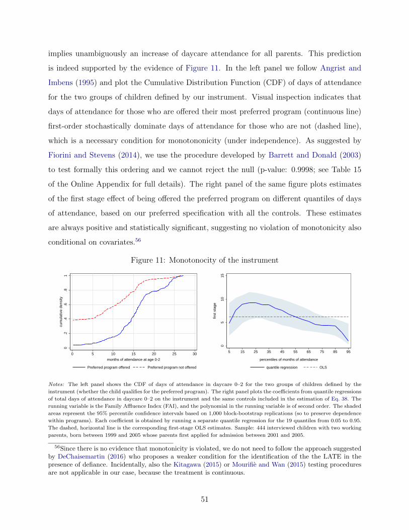
implies unambiguously an increase of daycare attendance for all parents. This prediction
is indeed supported by the evidence of Figure 11. In the left panel we follow Angrist and
Imbens (1995) and plot the Cumulative Distribution Function (CDF) of days of attendance
for the two groups of children defined by our instrument. Visual inspection indicates that
days of attendance for those who are offered their most preferred program (continuous line)
first-order stochastically dominate days of attendance for those who are not (dashed line),
which is a necessary condition for monotononicity (under independence). As suggested by
Fiorini and Stevens (2014), we use the procedure developed by Barrett and Donald (2003)
to test formally this ordering and we cannot reject the null (p-value: 0.9998; see Table 15
of the Online Appendix for full details). The right panel of the same figure plots estimates
of the first stage effect of being offered the preferred program on different quantiles of days
of attendance, based on our preferred specification with all the controls. These estimates
are always positive and statistically significant, suggesting no violation of monotonicity also
conditional on covariates.56
Figure 11: Monotonocity of the instrument
0.2
.4.6
.81
cum
ulat
ive
dens
ity
0 5 10 15 20 25 30
months of attendance at age 0-2
Preferred program offered Preferred program not offered
05
1015
first
sta
ge
5 15 25 35 45 55 65 75 85 95
percentiles of months of attendance
quantile regression OLS
Notes: The left panel shows the CDF of days of attendance in daycare 0–2 for the two groups of children defined by the
instrument (whether the child qualifies for the preferred program). The right panel plots the coefficients from quantile regressions
of total days of attendance in daycare 0–2 on the instrument and the same controls included in the estimation of Eq. 38. The
running variable is the Family Affluence Index (FAI), and the polynomial in the running variable is of second order. The shaded
areas represent the 95% percentile confidence intervals based on 1,000 block-bootstrap replications (so to preserve dependence
within programs). Each coefficient is obtained by running a separate quantile regression for the 19 quantiles from 0.05 to 0.95.
The dashed, horizontal line is the corresponding first-stage OLS estimates. Sample: 444 interviewed children with two working
parents, born between 1999 and 2005 whose parents first applied for admission between 2001 and 2005.
56Since there is no evidence that monotonicity is violated, we do not need to follow the approach suggestedby DeChaisemartin (2016) who proposes a weaker condition for the identification of the the LATE in thepresence of defiance. Incidentally, also the Kitagawa (2015) or Mourifie and Wan (2015) testing proceduresare not applicable in our case, because the treatment is continuous.
51

The first row of the left panel in Table 5 reports estimates of the Intention To Treat
(ITT) effect of just qualifying for the most preferred program in the interview sample.57
The specification in the first column includes only the polynomial g(yi). The second column
adds the application set characteristics, and the third one includes all controls. Note that
these ITT estimates are similar across columns. Taking the third column as the preferred
specification, the estimated ITT reveals that crossing the Preferred FAI threshold (i.e., hav-
ing a FAI barely sufficient to qualify for the preferred program), reduces total IQ by 3.0%.
This estimate is statistically different from zero (p-value: 0.005) and it is negative as the
numerical prediction (-1.8%) of the model in Section 6.2, when the observed distribution of
the FAI in the interview sample is used to weight the solutions computed for each specific
FAI level. Assuming that the model is a correct representation of reality, the two numbers
would coincide if the distribution of FAI levels at each Preferred thresholds corresponded to
the distribution of FAI levels in the interview sample.
First stage estimates are reported in the second row of Table 5.58 Just qualifying for the
preferred program increases daycare 0–2 attendance by about six months. The F-test statistic
on the excluded instrument is sufficiently large in all specifications and samples, suggesting
that weak instruments are not a concern.59 Rescaling the ITT effect by the first stage gives
the IV estimate of the effect of one month of daycare 0–2 attendance. In our preferred
specification (third column), and similarly in the others, this is a statistically significant loss
of about 0.5% (p-value: 0.004) which, at the sample mean (116.4), corresponds to 0.6 IQ
points and to 4.5% of the IQ standard deviation.
Table 6 offers a check on the parametric assumptions underlying Table 5, using the
57 Specifically, we estimate the following reduced form equation,
θi = α+ βPi + g(yi) + γAi + δXi + εi,
where g(yi) is a second order polynomial in the FAI and β is the Intention-To-Treat (ITT) effect.58 In this case, we estimate the first stage equation,
τd,i = α+ βPi + g(yi) + γAi + δXi + εi,
where g(yi) is a second order polynomial in FAI and β is the first stage estimate.59In the Basket 4 universe described by the right panel of Figure 4, crossing the preferred threshold from
higher to lower FAI implies an increase of only about three months of daycare attendance. The fact that inthe interview sample, as shown also by Figure 10, the first stage is larger is due to the differences betweenthis sample and the universe discussed in Section 5.
52

Tab
le5:
Eff
ects
ofday
care
0–2
atte
ndan
ceon
IQ,
for
all
childre
nan
dby
leve
lof
the
Pre
ferr
edFA
Ith
resh
old
Dep
enden
tva
riab
le:
ln(I
Q)
All
FA
Ith
resh
olds
FA
Ith
resh
olds≤
med
ian
FA
Ith
resh
olds>
med
ian
(mea
nth
resh
old:e
24.7
k)
(mea
nth
resh
old:e
16.4
k)
(mea
nth
resh
old:e
33.0
k)
ITT
effec
tof
qual
ifyin
g-0
.026
*-0
.030
**-0
.030
**-0
.005
-0.0
12-0
.009
-0.0
56**
-0.0
60**
-0.0
65**
for
the
pre
ferr
edpro
gram
(0.0
10)
(0.0
11)
(0.0
10)
(0.0
15)
(0.0
15)
(0.0
14)
(0.0
18)
(0.0
19)
(0.0
18)
Fir
stst
age:
effec
tof
qual
ifyin
g6.
3**
6.4*
*5.
9**
5.9*
*5.
1**
5.8*
*4.
6**
4.8*
*4.
6**
onm
onth
sof
atte
ndan
ce(0
.9)
(0.9
)(0
.9)
(1.3
)(1
.4)
(1.4
)(1
.3)
(1.4
)(1
.3)
IVeff
ect
ofon
em
onth
-0.0
04**
-0.0
05**
-0.0
05**
-0.0
01-0
.002
-0.0
02-0
.012
**-0
.012
**-0
.014
**of
day
care
atte
ndan
ce(0
.002
)(0
.002
)(0
.002
)(0
.003
)(0
.002
)(0
.002
)(0
.004
)(0
.004
)(0
.005
)
F-s
tat
onex
cluded
inst
rum
ents
49.1
46.9
44.8
22.0
18.0
13.8
12.9
12.3
12.3
Num
ber
ofob
serv
atio
ns
444
444
444
228
228
228
216
216
216
Pol
ynom
ial
inFA
IY
esY
esY
esY
esY
esY
esY
esY
esY
esA
pplica
tion
set
contr
ols
Yes
Yes
Yes
Yes
Yes
Yes
Pre
-tre
atm
ent
contr
ols
Yes
Yes
Yes
Notes:
Th
eta
ble
rep
ort
sp
ara
met
ric
esti
mate
sof
the
effec
tof
on
em
onth
of
dayca
re0–2
on
log
IQ,
an
dth
eass
oci
ate
dIT
Tan
dfi
rst
stage,
at
all
level
sof
the
Pre
ferr
edFA
I
thre
shold
an
dse
para
tely
for
Pre
ferr
edFA
Ith
resh
old
sb
elow
or
ab
ove
the
med
ian
Pre
ferr
edFA
Ith
resh
old
.IT
Tco
effici
ents
are
from
regre
ssio
ns
of
log
IQon
the
inst
rum
ent
(wh
eth
erth
ech
ild
qu
alifi
esfo
rth
ep
refe
rred
pro
gra
m)
an
dco
ntr
ols
.F
irst
-sta
ge
coeffi
cien
tsare
from
regre
ssio
ns
of
month
s(1
month
=20
days
of
att
end
ance
)sp
ent
ind
ayca
re
0–2
on
the
inst
rum
ent
an
dco
ntr
ols
.IV
coeffi
cien
tsare
from
regre
ssio
ns
of
log
IQon
month
sof
att
end
an
cean
dco
ntr
ols
usi
ng
ad
um
my
for
qu
ali
fica
tion
inth
ep
refe
rred
pro
gra
m
as
the
inst
rum
ent.
Th
eru
nn
ing
vari
ab
leis
the
Fam
ily
Affl
uen
ceIn
dex
(FA
I),
an
dth
ep
oly
nom
ial
inth
eru
nn
ing
vari
ab
leis
of
seco
nd
ord
er.
Sam
ple
:444
inte
rvie
wed
child
ren
wit
htw
ow
ork
ing
pare
nts
,b
orn
bet
wee
n1999
an
d2005,
wit
hn
on
-mis
sin
gou
tcom
eor
covari
ate
san
dw
hose
pare
nts
firs
tap
plied
for
ad
mis
sion
tod
ayca
reb
etw
een
2001
an
d
2005.
Rob
ust
stan
dard
erro
rsin
pare
nth
eses
,cl
ust
ered
at
the
faci
lity
level
.*
sign
ifica
nt
at
5%
;**
sign
ifica
nt
at
1%
or
bet
ter.
53

methodology suggested in Calonico et al. (2014b).
Column 1 shows non-parametric estimates for the whole interview sample, based on a
triangular kernel and a local polynomial of degree zero with optimal bandwith selection.60
Results are in line with those of the left panel in Table 5 although less statistically significant
given the small sample size. The ITT effect of just qualifying for the preferred program is
estimated to be a loss of 2.8% (it is 3.0% in Table 5). The non-parametric first stage estimate
is slightly lower than the parametric one as well (4.6 instead of 6.3 months). As for the IV
estimate, both the conventional and the bias-corrected non-parametric estimators suggested
by Calonico et al. (2014b) imply a 0.6% IQ loss induced by one additional month of daycare
0–2 (which is slightly higher than the 0.5% parametric loss reported in Table 5).
As argued in Section 5, the interview sample is characterized by relatively affluent and
educated parents in one of the richest Italian cities. Therefore, in light of Remark 2, it should
not come as a surprise that the effect of daycare, for children who increase attendance because
their parents are offered their most preferred program as opposed to a less preferred one,
is estimated to be negative in this population. To further probe the empirical validity of
the prediction in Remark 2, we separate children in two groups according to whether the
Preferred threshold to which they are associated is above or below the median of all Preferred
thresholds. Results are reported in the middle and right panels of Table 5.61 For the less
affluent group, below the median, the estimates refer to the effect of daycare 0–2 around a
Preferred threshold of e16.4k on average (corresponding to a gross annual family income of
about e43k), while in the more affluent group above the median the average threshold is
e33.0k (annual family income of about e88k). The numerical solution of the model described
in Section 6.2 suggests that the level of FAI above which the IQ effect induced by the offer
of the most preferred program turns from positive to negative is about e18k. Therefore, we
expect the estimates for the less affluent group to be close to zero or even slightly positive,
while those for the more affluent group should be unambiguously negative.
60Estimates based on a higher order local polynomial, which according to Imbens and Lemieux (2008)should be preferable in this context, are unstable and not reliable. Since the non-parametric analysis isimplemented on stacked and centered thresholds, here we drop observations located at zero distance fromthresholds for the reasons discussed in Fort et al. (2017). See the note to the table for further details.
61 The Online Appendix reproduces the figure and tables of the main text supporting the validity ofour identification strategy separately for the two affluence groups. All the available covariates are perfectlybalanced and continuous at the thresholds in both cases.
54

Table 6: Effects of daycare 0–2 attendance on IQ: nonparametric estimates.
Preferred thresholds All ≤ median > median All AllGender All All All Girls Boys
ITT of just -0.028 0.0324 -0.0791+ -0.037 -0.011qualifying (0.020) (0.033) (0.032) (0.026) (0.041)
First stage 4.6∗∗ 3.8∗ 4.9∗∗ 3.8∗ 6.2∗
(1.3) (1.8) (2.2) (1.7) (2.4)robust p-value 0.045 0.213 0.289 0.485 0.055
Effect of 1 month -0.006 0.009 -0.016∗ -0.010 -0.002(conventional) (0.005) (0.010) (0.008) (0.008) (0.007)
Effect of 1 month -0.006 0.014 -0.023∗∗ -0.015+ -0.001(bias-corrected) (0.005) (0.010) (0.008) (0.008) (0.007)
Effect of 1 month -0.006 0.014 -0.023∗ -0.015 -0.001(robust) (0.006) (0.013) (0.011) (0.011) (0.009)
Bandwith for Loc. Poly (h) 6.544 3.094 7.691 7.076 5.088Bandwith for bias (b) 16.351 7.039 16.780 16.297 10.820Number of observations 150 45 78 91 46
Notes: The table reports nonparametric estimates of the effect of one month of daycare 0–2 on the log of IQ, with related ITT
and first stage. The methodology used is detailed in Calonico et al. (2014b), and it is implemented using the software described
in Calonico et al. (2014a). The grade of local polynomials is zero and the kernel is triangular. The table also reports the optimal
bandwidths for the local polynomial (h) and for the bias (b) as well as the p-value from a test for the null hypothesis that the
first stage coefficient is zero, obtained using a robust and bias corrected estimator for the first stage. The ITT and first stage
estimates are obtained using the conventional nonparametric estimator. The effects of one month of daycare 0–2 are obtained
using three distinct RD estimators: the local polynomial estimator (conventional), the bias-corrected estimator proposed by
Calonico et al. (2014b) and the bias-corrected estimator with robust standard errors. The running variable is the Family
Affluence Index (FAI). Sample: interviewed children with two working parents, born between 1999 and 2005, with non-missing
outcome or covariates and whose parents first applied for admission to daycare between 2001 and 2005. + significant at 10%;
* significant at 5%; ** significant at 1% or better.
55

The top panel of Figure 12 offers a graphical confirmation of these predictions. While
the LLR fit for the more affluent group shows a negative jump of child IQ when the FAI
crosses Preferred thresholds from higher to lower values (left to right), for the less affluent
group, the jump is positive and smaller in size.
Figure 12: Full scale IQ around Preferred FAI thresholds, by family affluence and by gender
9010
011
012
013
014
0
full
scal
e IQ
-50 -40 -30 -20 -10 0 10 20 30 40 50
distance from FAI threshold
Less affluent
9010
011
012
013
014
0
full
scal
e IQ
-50 -40 -30 -20 -10 0 10 20 30 40 50
distance from FAI threshold
More affluent
9010
011
012
013
014
0
full
scal
e IQ
-50 -40 -30 -20 -10 0 10 20 30 40 50
distance from FAI threshold
Boys90
100
110
120
130
140
full
scal
e IQ
-50 -40 -30 -20 -10 0 10 20 30 40 50
distance from FAI threshold
Girls
Notes: The dots represent average IQ inside e2k bins, plotted as a function of the distance (thousands of real e) of a child’s
FAI from her Preferred FAI threshold, by family affluence (top panel) and by gender (bottom panel). The size of a circle is
proportional to the number of observations in the corresponding e2k bin. “Less affluent” and “More affluent” are observations
associated with Preferred FAI thresholds below or above the median Preferred FAI threshold, respectively. The bold lines are
LLR on the underlying individual observations, with a triangular kernel and optimal bandwidth selection, from Calonico et al.
(2014b). FAI stands for Family Affluence Index. Sample: 373 interviewed children with two working parents, born between
1999 and 2005 whose parents first applied for admission between 2001 and 2005 to programs with rationing, whose FAI distance
from the Final FAI thresholds is at most e50k and, for the reasons discussed in Fort et al. (2017), is different from zero.
Parametric estimates of these jumps are reported in the top row of the middle and right
panels of Table 5. In the less affluent group, the ITT effect of just qualifying for the most
preferred program is estimated to be negative but very small. In the more affluent group
the estimate is similarly negative, but about 5 time larger (-5–6%) and very precise. The
second row in the same panels of Table 5 displays the first stage effect and confirms another
prediction of the model described in Section 6. As implied by Remark 1 the first stage is
smaller for more affluent parents (about 4.7 vs. 5.7 months). Rescaling the ITT effect by the
56

first stage gives a statistically significant IV estimate for β of about -1.2–1.4% in the more
affluent group, while for less affluent households the estimate is essentially null. A similar
pattern emerges in the nonparametric estimates for the two groups reported in columns 2
and 3 of Table 6.
8 Suggestions from the psychological literature
Psychologists have produced persuasive empirical evidence that one-to-one interactions with
adults (more than interactions with peers) are a crucial input for cognitive development in
the first three years of life of a child. For instance, in an empirical field study of 42 American
families, Hart and Risley (1995) have recorded one full hour of words spoken at home every
month for two and a half years by parents with their children at age 0–2. They conclude that
“the size of the children’s recorded vocabularies and their IQ scores were strongly associated
with the size of their parents’ recorded vocabulary and their parents’ scores on a vocabulary
pre-test” (p. 176). Along the same lines, Rowe and Goldin-Meadow (2009) and Cartmill
et al. (2013) show that the quality of parental input in the first three years of life (e.g. in
terms of parental gesture and talking) improves children’s vocabulary before school entry.
Similarly, Gunderson et al. (2013) finds that parental praise directed to 1-3 years old children
predicts their motivation five years later.62
What is perhaps even more interesting is why, according to psychologists, these one-to-one
interactions with adults early in life are so important. A fascinating theory has been proposed
by Csibra and Gergely (2009, 2011). According to these authors, the communication between
a trusted adult and a child allows the latter to understand more rapidly if an experience has
a general value or only a specific value. In the absence of such communication the child has
to repeat and confirm the experience many times in order to assess its general or particular
validity (very much like in a sort of statistical inference requiring a large sample). An adult,
62Related to these results, psychologists (like economists, see footnote 9), have estimated negative effectsof increasing parental working time (in particular maternal) on cognitive, non-cognitive and behavioraloutcomes of children. See, for example, Brooks-Gunn and Waldfogel (2002), Adi-Japha and Klein (2009),McPherran Lombardi and Levine Coley (2014) and the meta-analysis in Li et al. (2013). Different from theeconomic literature, however, most of these studies are observational and do not exploit quasi-experimentalidentification strategies.
57

instead, can quickly inform the child on the nature of what he or she is experimenting. If
the adult can be trusted, then the child can save time and move on to other experiences,
thus gaining an advantage in terms of cognitive development.
The focus on one-to-one interactions in our context is relevant because, as noted by
Clarke-Stewart et al. (1994), infants and toddlers generally experience less one-to-one atten-
tion in daycare than at home because at home they are typically taken care of by a parent,
a grandparent, or a nanny. Under these care modes a child receives attention in a 1:1 ratio,
possibly somewhat worse if, for example, siblings are present. This is precisely the case for
the children in our sample. When we asked their parents which options were available at the
time of the first application as an alternative to daycare during the workday, 50.5% checked
“the mother”, 11% “the father”, 44.8% “the grandparents”, 4.5% “other family members”,
18.9% “a babysitter or a nanny”, and only 12.1% checked “some other daycare center” (mul-
tiple answers were possible).63 The adult-to-child ratio in daycare 0–2 depends instead on
the specific institutional setting. At the BDS, during the period under investigation, this
ratio was 1:4 at age 0 and 1:6 at age 1–2. This may be part of the reason why, different from
us as explained in Section 2, both Felfe and Lalive (2014) and Drange and Havnes (2015)
find positive effects of daycare 0–2 in Germany and Norway. In their institutional setting,
the adult-to-child ratio is about 1:3, much closer to a family environment.
A related claim that psychologists have supported with persuasive empirical evidence is
that girls are more “mature” than boys, in the sense of being more capable of absorbing
cognitive stimuli at an early age. For example, Fenson et al. (1994) study 1,800 toddlers
(16-30 months of age) finding that girls perform better in lexical, gestural, and grammatical
development. Galsworthy et al. (2000) examine about 3,000 2-year-old twin pairs and show
63In Bologna there are very few private daycare facilities outside the public system. The reason is thatBologna is one of the Italian cities with the largest and most highly-reputed public daycare systems, whichleaves little room for independent private providers, relative to other cities. The BDS includes 8 charterfacilities (offering 40 programs) that are privately managed but strictly regulated by the BDS. According tothe reputational indicator of quality described in Section 3, these charter programs are perceived by parentsas worse than the non-charter ones. On average, for given distance, charter programs are ranked 0.43positions lower than the non-charter ones if they are included in the application set of a parent. Moreover,the probability that a charter program is not ranked by parents in their application set is higher than fornon-charter ones (0.95 vs.0.91). The odds that a charter program is ranked first by a parent is 0.007 whilethe odds that a program is charter is 0.046. Therefore, it is unlikely that the worse quality of these charterprograms is responsible for the negative IQ effect that we estimate – which derives from the offer of the mostpreferred program to a parent. If anything, their presence should reduce the absolute size of our estimates.
58

that girls score higher on verbal and non-verbal cognitive ability. The longitudinal study of
Bornstein et al. (2004) on 329 children observed between age 2 and 5 reaches similar con-
clusions for an age range partially overlapping with ours: they show that “girls consistently
outperformed boys in multiple specific and general measures of language” (p. 206).
If girls at age 0–2 are relatively more capable of making good use of stimuli that improve
their skills, then their development is hurt (more than for boys) by an extended exposure
to daycare because it implies fewer one-to-one interactions with adults, and these are more
valuable for their cognitive development. In Section 6.1.4, we have proposed a model of how
parental decisions concerning child care are compatible with these gender differences in the
effects of daycare 0–2 .
The lower panel or Figure 12 provides a graphical description of how IQ changes around
Preferred FAI thresholds, separately by gender. While the LLR fit for boys is continuous
when the FAI crosses the Preferred threshold from higher to lower values (left to right), for
girls we observe a negative jump. Girls with a FAI small enough to just qualify for their
most preferred program have a lower IQ with respect to girls who barely do not.64
This finding is confirmed by the parametric estimation of Eq. 38, separately for boys and
girls. Results are reported in Table 7, for the same three specifications already considered
in Table 5. In our preferred specification, which includes all controls in the third and sixth
columns, the ITT effect of just qualifying for the most preferred program is a statistically
significant IQ loss of about 3.9% for girls (p-value: 0.017), while for boys it is smaller and
we cannot reject the hypothesis that it is equal to zero. A similar gender difference emerges
also from the IV estimates, which indicate that for girls one additional month in daycare
0–2 reduces IQ by 0.7% (p-value: 0.016), while the effect for boys is almost half this size and
is again not statistically different from zero.65 The middle panel shows that the gender gap
64We can easily dismiss the possibility that this gender heterogeneity in the effects of daycare 0–2 reflectsdifferences in pre-treatment characteristics of boys and girls in our sample: the Online Appendix reproduces,separately by gender, the figures and tables reported here supporting the validity of our identification strategy.All the available covariates as well as treatment intensity are balanced and continuous at the thresholds forboth genders. Similar across genders are also the answers given by parents to the question concerningalternative modes of care.
65Interestingly, in a longitudinal study of 113 first-born preschool children, 58 girls and 55 boys, Bornsteinet al. (2006) find, in line with our results, that “Girls who had greater amount of non-maternal care frombirth to 1 year scored lower on the Spoken Language Quotient at preschool” (pag. 145).
59

in the ITT is not due to differences in the first stage. For both boys and girls, attendance
in daycare 0–2 increases by approximately 6 months when the FAI crosses the Preferred
threshold from higher to lower values. A qualitatively similar gender difference in the effects
of IQ emerges from the non-parametric estimates reported in columns 4 and 5 of Table 6
where, if anything, the losses for girls appear to be even larger.
Table 7: Gender heterogeneity of the IQ effects of daycare 0–2
Dependent variable: ln(IQ)
Boys Girls
ITT effect of qualifying -0.013 -0.018 -0.023 -0.040** -0.043** -0.039**for the preferred program (0.016) (0.016) (0.016) (0.015) (0.016) (0.016)
First stage: effect of qualif. 6.11** 6.68** 6.32** 6.54** 6.42** 5.60**on months of attendance (0.98) (0.93) (0.89) (1.12) (1.19) (1.19)
IV effect of one month -0.002 -0.003 -0.004 -0.006* -0.007* -0.007**of daycare attendance (0.003) (0.002) (0.002) (0.002) (0.003) (0.003)
F-stat on excluded instrum. 38.9 51.1 50.6 33.9 29.0 22.1Number of observations 215 215 215 229 229 229
Polynomial in FAI Yes Yes Yes Yes Yes YesAppl. set controls Yes Yes Yes YesPre-treat. controls Yes Yes
Notes: The table reports parametric estimates of the effect of one month of daycare 0–2 on log IQ, and the associated ITT
and first stage, by gender. First-stage coefficients are from regressions of months (1 month = 20 days of attendance) spent in
daycare 0–2 on the instrument and controls, as in equation (58). IV coefficients are from regressions of log IQ on months of
attendance and controls, as in equation (38), using a dummy for qualification in the preferred program as the instrument. The
running variable is the Family Affluence Index (FAI), and the polynomial in the running variable is of second order. Sample:
interviewed children with two working parents, born between 1999 and 2005, with non-missing outcome or covariates and whose
parents first applied for admission to daycare between 2001 and 2005. Robust standard errors in parentheses, clustered at the
facility level. * significant at 5%; ** significant at 1% or better.
This gender difference in the cognitive losses induced by daycare attendance supports the
relevance of one-to-one interactions with adults as an explanation of our results.66
66We have also explored the possibility that the loss suffered by girls depend on sex ratios within each
60

9 Conclusions
This paper joins a growing literature studying the effects of time spent in daycare 0–2 for
children in advantaged families. We study the offspring of dual-earner households with
cohabiting parents in Bologna, one of the most educated and richest Italian cities with
a highly reputed public daycare system. For the children in this population, our results
indicate a quantitatively and statistically significant IQ loss at age 8–14. This loss is even
more pronounced when, within this population, we look at children with relatively more
affluent parents. These are typically the relevant marginal subjects to be considered in an
evaluation of daycare expansions for the worldwide increasing community of families in which
both parents want to work.
We interpret this findings in a theoretical model showing that, when offered the most
preferred daycare program as opposed to a less preferred one, relatively affluent parents take
advantage of this opportunity to increase daycare attendance of their children and so work
more or reduce costly market care. This increase in attendance is smaller than the analogous
one occurring in a less affluent household, but due to a higher earning potential it generates
an increase of family resources that is large enough to become attractive even if it comes at
the cost of a decrease in child IQ.
These results seem relevant not only because of their novelty with respect to the liter-
ature, but also because they implicitly support the hypothesis, suggested by psychologists,
according to which the sign and size of the effects of daycare 0–2 are mostly driven by three
factors. First, whether this early life experience deprives children of one-to-one interactions
with adults at home. Second, by the quality of these interactions, which is likely to be higher
in more affluent households. And, third, by whether children can make good use of them.
program. Psychologists have observed that in early education “(T)eachers spend more time socializing boysinto classroom life, and the result is that girls get less teacher attention. Boys receive what they need ...Girls’ needs are more subtle and tend to be overlooked.” (Koch, 2003, p. 265). However, we do not findany evidence that sex ratios affect the size of the effects for girls and boys, possibly because the variationin these ratios is quite small for the children in our sample. Moreover, the data do not support anotherpossible hypothesis according to which gender differences in breastfeeding explain the gender gap in theeffects of daycare. The duration of breastfeeding has been shown to be positively associated with cognitiveoutcomes (Anderson et al., 1999; Borra et al., 2012; Fitzsimons and Vera-Hernandez, 2013), and early daycareenrollment or attendance may shorten it. However, we find no effect (and specifically no differential effectby gender) of days in daycare on the duration of breastfeeding.
61

The latter claim is supported by the finding that daycare 0–2 has a more negative effect
on the IQ of girls, in combination with the psychological evidence suggesting that girls are
developed enough at this young age to exploit high quality interactions with adults that for
boys are less valuable.
Our identification strategy exploits affluence thresholds that discriminate between similar
parents whose children attend daycare 0–2 for longer versus shorter periods because they
are barely admitted to their preferred program instead of being just excluded from it. This
strategy makes our results valuable not only for parents but also for policy makers interested
in expanding vacancies in the daycare systems under their jurisdiction. Our estimates speak
precisely about the effect of such a policy, which would allow more affluent children to attend
for a longer time in programs that they prefer more, with negative effects on their IQ that
may not be socially optimal even if the utility of their parents increases.
62

References
Abdulkadiroglu, A., Angrist, J. D., Narita, Y., Pathak, P. A., 2015, Research design meetsmarket design: Using centralized assignment for impact evaluation, Working Paper 21705,National Bureau of Economic Research.
Abdulkadirolu, A., Angrist, J., Pathak, P., 2014, The Elite Illusion: Achievement Effects atBoston and New York Exam Schools, Econometrica 82, 137–196.
Adi-Japha, E., Klein, P. S., 2009, Relations Between Parenting Quality and Cognitive Per-formance of Children Experiencing Varying Amounts of Childcare, Child Development 80,893–906.
Almond, D., Currie, J., 2011, Human Capital Development Before Age Five, volume 4, PartB of Handbook of Labor Economics, 1315 – 1486, Elsevier.
Anderson, J. W., Johnstone, B. M., Remley, D. T., 1999, Breast-feeding and cognitivedevelopment: a meta-analysis, The American Journal of Clinical Nutrition 70, 525–535.
Anderson, M. L., 2008, Multiple Inference and Gender Differences in the Effects of EarlyIntervention: A Reevaluation of the Abecedarian, Perry Preschool, and Early TrainingProjects, Journal of the American Statistical Association 103, 1481–1495.
Angrist, J., Imbens, G., 1995, Two-Stage Least Squares Estimation of Average Causal Ef-fects in Models with Variable Treatment Intensity, Journal of the American StatisticalAssociation 90, 431–442.
Baker, M., Gruber, J., Milligan, K., 2008, Universal Child Care, Maternal Labor Supply,and Family Well-Being, Journal of Political Economy 116, 709–745.
Baker, M., Gruber, J., Milligan, K., 2015, Non-Cognitive Deficits and Young Adult Out-comes: The Long-Run Impacts of a Universal Child Care Program, Working Paper 21571,National Bureau of Economic Research.
Barrett, G. F., Donald, S. G., 2003, Consistent Tests For Stochastic Dominance, Economet-rica 71, 71–104.
Becker, G. S., 1965, A Theory of the Allocation of Time, The Economic Journal 75, 493–517.
Bellettini, G., Taddei, F., Zanella, G., 2017, Intergenerational altruism and house prices:Evidence from bequest tax reforms in Italy, European Economic Review 92, 1 – 12.
Belsky, J., 1988, The effects of infant day care reconsidered, Early Childhood ResearchQuarterly 3, 235 – 272.
Belsky, J., 2001, Emanuel Miller Lecture: Developmental risks (still) associated with earlychild care, Journal of Child Psychology and Psychiatry 42, 845–859.
Belsky, J., Steinberg, L. D., 1978, The effects of day care: A critical review, Child Develop-ment 49, 929–949.
Bernal, R., 2008, The effect of maternal employment and child care on children’s cognitivedevelopment, International Economic Review 49, 1173–1209.
63

Bernal, R., Keane, M. P., 2011, Child Care Choices and Children’s Cognitive Achievement:The Case of Single Mothers, Journal of Labor Economics 29, pp. 459–512.
Bertanha, M., 2016, Regression Discontinuity Design with Many Thresholds, Mimeo.
Borghans, L., Duckworth, A. L., Heckman, J. J., ter Weel, B., 2008, The Economics andPsychology of Personality Traits, Journal of Human Resources 43, 972–1059.
Bornstein, M., Hahn, C.-S., Gist, N., Haynes, M., 2006, Long term cumulative effects ofchildcare on children’s mental development and socioemotional adjustment in a non-risksample: the moderating effects of gender, Early Child Development and Care 176, 129–156.
Bornstein, M. H., Hahn, C.-S., Haynes, O. M., 2004, Specific and general language perfor-mance across early childhood: Stability and gender considerations, First Language 24,267–304.
Borra, C., Iacovou, M., Sevilla, A., 2012, The effect of breastfeeding on children’s cognitiveand noncognitive development , Labour Economics 19, 496 – 515.
Brooks-Gunn, Jeanne, W.-J. H., Waldfogel, J., 2002, Maternal Employment and Child Cog-nitive Outcomes in the First Three Years of Life: The NICHD Study of Early Child Care,Child Development 73, 1052?1072.
Calonico, S., Cattaneo, M. D., Titiunik, R., 2014a, Robust Data Driven Inference in theRegression-Discontinuity Design, The Stata Journal 14, 909–946.
Calonico, S., Cattaneo, M. D., Titiunik, R., 2014b, Robust Nonparametric Confidence In-tervals for Regression-Discontinuity Designs, Econometrica 82, 2295–2326.
Campbell, F. A., Ramey, C. T., 1994, Effects of Early Intervention on Intellectual andAcademic Achievement: A Follow-up Study of Children from Low-Income Families, ChildDevelopment 65, 684–698.
Carneiro, P., Cunha, F., Heckman, J., 2003, Interpreting The Evidence of Family Influenceon Child Development, Mimeo.
Carneiro, P., Ginja, R., 2014, Long-Term Impacts of Compensatory Preschool on Healthand Behavior: Evidence from Head Start, American Economic Journal: Economic Policy6, 135–73.
Carneiro, P., Løken, K. V., Salvanes, K. G., 2015, A Flying Start? Maternity Leave Benefitsand Long-Run Outcomes of Children, Journal of Political Economy 123, pp. 365–412.
Cartmill, E., Armstrong, B., Gleitman, L., Goldin-Meadow, S., Medina, T., Trueswell, J.,2013, Quality of early parent input predicts child vocabulary 3 years later, PNAS 110, pp.11278–11283.
Cattaneo, M., Keele, L., Titiunik, R., Vazquez-Bare, G., 2016, Interpreting Regression Dis-continuity Designs with Multiple Cutoffs, Mimeo.
Clarke-Stewart, K., Gruber, C., Fitzgerald, L., 1994, Children at home and in day care , L.Erlbaum Associates, Hillsdale, NJ.
64

Comune di Bologna, 2010, Progetto pedagogico del nido d’infanzia del Comune diBologna, Report: Comune di Bologna- Settore Istruzione.
Csibra, G., Gergely, G., 2009, Natural Pedagogy, Philosophical Transactions of the RoyalSociety B 13, 148–153.
Csibra, G., Gergely, G., 2011, Natural Pedagogy as evolutionary adaptation, Trends inCognitive Sciences 366, 1149–1157.
Cunha, F., Heckman, J., 2007, The Technology of Skill Formation, American EconomicReview 97, 31–47.
Cunha, F., Heckman, J. J., Schennach, S. M., 2010, Estimating the Technology of Cognitiveand Noncognitive Skill Formation, Econometrica 78, pp. 883–931.
Currie, J., 2001, Early Childhood Education Programs, Journal of Economic Perspectives15, 213–238.
DeChaisemartin, C., 2016, Tolerating Defiance? Local Average Treatment Effects WithoutMonotonicity, Quantitative Economics, forthcoming .
Del Boca, D., Pronzato, C., Sorrenti, G., 2015, When rationing plays a role: selection criteriain the Italian early child care system, Carlo Alberto Notebooks 399, Collegio Carlo Alberto.
Drange, N., Havnes, T., 2015, Child Care Before Age Two and the Development of Languageand Numeracy: Evidence from a Lottery, IZA Discussion Papers 8904, Institute for theStudy of Labor (IZA).
Duncan, G. J., Magnuson, K., 2013, Investing in Preschool Programs, Journal of EconomicPerspectives 27, 109–32.
Dustmann, C., Raute, A., Schonberg, U., 2013, Does Universal Child Care Matter? Evidencefrom a Large Expansion in Pre-School Education, Mimeo.
Elango, S., Garca, J. L., Heckman, J. J., Hojman, A., 2015, Early childhood education,Working Paper 21766, National Bureau of Economic Research.
Felfe, C., Lalive, R., 2014, Does Early Child Care Help or Hurt Childrens’s Development?,IZA Discussion Papers 8484, Institute for the Study of Labor (IZA).
Felfe, C., Nollenberger, N., Rodrguez-Planas, N., 2015, Cant Buy Mommys Love? Univer-sal Childcare and Children’s Long-Term Cognitive Development, Journal of PopulationEconomics 28, 393–422.
Fenson, L., Dale, P. S., Reznick, J. S., Bates, E., Thal, D. J., Pethick, S. J., Tomasello,M., Mervis, C. B., Stiles, J., 1994, Variability in Early Communicative Development,Monographs of the Society for Research in Child Development 59, pp. i+iii–v+1–185.
Fiorini, M., Stevens, K., 2014, Assessing the Monotonicity Assumption in IV and FuzzyRDD Designs, Economics Working Paper Series- University of Sidney 2014-13.
Fitzsimons, E., Vera-Hernandez, M., 2013, Food for Thought? Breastfeeding and ChildDevelopment, IFS Working Papers (W13/31).
65

Fort, M., Ichino, A., Rettore, E., Zanella, G., 2017, On the Perils of Stacking Thresholds inRD Designs, Mimeo.
Fort, M., Ichino, A., Zanella, G., 2016, Daycare 0-2 for Children: Does Early DaycareImprove Children’s Outcomes?, Report prepared for the Fondazione Rodolfo DeBenedetti.
Gale, D., Shapley, L., 1962, College Admissions and the Stability of Marriage, AmericanMathematical Monthly 69, pp. 9–15.
Galsworthy, M. J., Dionne, G., Dale, P. S., Plomin, R., 2000, Sex differences in early verbaland non-verbal cognitive development, Developmental Science 3, 206–215.
Garber, H., 1988, The Milwaukee Project: Preventing Mental Retardation in Children AtRisk, Technical report, American Association on Mental Retardation.
Gottfredson, L. S., 1997, Mainstream science on intelligence: An editorial with 52 signatories,history, and bibliography, Intelligence 24, 13 – 23, special Issue Intelligence and SocialPolicy.
Gunderson, E. A., Gripshover, S. J., Romero, C., Dweck, C. S., Goldin-Meadow, S., Levine,S. C., 2013, Parent praise to 1- to 3-year-olds predicts children’s motivational frameworks5 years later, Child Development 84, 1526–1541.
Hahn, J., Todd, P., Van der Klaauw, W., 2001, Identification and Estimation of TreatmentEffects with a Regression Discontinuity Design, Econometrica 69, 201–209, notes andComments.
Hart, B., Risley, T., 1995, Meaningful Differences in the Everyday Experience of YoungAmerican Children , Brookes Publishing Co., Baltimore MD.
Havnes, T., Mogstad, M., 2015, Is Universal Child Care Leveling the Playing Field?, Journalof Public Economics 127, 100 – 114.
Heckman, J. J., Mosso, S., 2014, The Economics of Human Development and Social Mobility,Annual Review of Economics 27, 109–32.
Heckman, J. J., Urzua, S., Vytlacil, E., 2006, Understanding Instrumental Variables inModels with Essential Heterogeneity, The Review of Economics and Statistics 88, 389–432.
Herbst, C. M., 2013, The Impact of Non-Parental Child Care on Child Development: Evi-dence from the Summer Participation Dip, Journal of Public Economics 105, 86 – 105.
Hewett, V., 2001, Examining the Reggio Emilia Approach to Early Childhood Education,Early Childhood Education Journal 29, 95–100.
Imbens, G. W., Lemieux, T., 2008, Regression discontinuity designs: A guide to practice,Journal of Econometrics 142, 615–635.
Kitagawa, T., 2015, A test for instrument validity, Econometrica 83, 2043–2063.
Koch, J., 2003, Gender Issues in the Classroom, in: Reynolds, W. M., Miller, G. E. (eds.),Handbook of Psychology, volume 7 (Educational Psychology), 259–284, Wiley.
66

Kottelenberg, M. J., Lehrer, S. F., 2014a, Do the perils of universal childcare depend on thechilds age?, CESifo Economic Studies 60, 338–365.
Kottelenberg, M. J., Lehrer, S. F., 2014b, The Gender Effects of Universal Child Care inCanada: Much ado about Boys?, Mimeo.
Kottelenberg, M. J., Lehrer, S. F., 2017, Targeted or universal coverage? assessing hetero-geneity in the effects of universal childcare, Journal of Labor Economics 35.
Lalive, R., Zweimuller, J., 2009, How does parental leave affect fertility and return to work?evidence from two natural experiments, The Quarterly Journal of Economics 124, 1363.
Lee, D. S., Lemieux, T., 2010, Regression discontinuity designs in economics, Journal ofEconomic Literature 48, 281–355.
Li, J., Johnson, S. E., Han, W.-J., Andrews, S., Kendall, G., Strazdins, L., Dockery, A.,2013, Parents’ nonstandard work schedules and child well-being: A critical review of theliterature, The Journal of Primary Prevention 35, 53–73.
Magnuson, K. A., Ruhm, C., Waldfogel, J., 2007, Does prekindergarten improve schoolpreparation and performance?, Economics of Education Review 26, 33–51.
McCrary, J., 2008, Manipulation of the Running Variable in the Regression DiscontinuityDesign: A Density Test, Journal of Econometrics 142, 698–714.
McPherran Lombardi, C., Levine Coley, R., 2014, Early Maternal Employment and ChildrensSchool Readiness in Contemporary Families, Developmental Psychology 50, 2071–2084.
Mourifie, I., Wan, Y., 2015, Testing local average treatment effects assumptions, Mimeo,University of Toronto.
Noboa-Hidalgo, G. E., Urza, S. S., 2012, The Effects of Participation in Public Child CareCenters: Evidence from Chile, Journal of Human Capital 6, 1 – 34.
Puma, M., Bell, S., Cook, R., Heid, C., Broene, P., Jenkins, F., Mashburn, A., Downer, J.,2012, Third Grade Follow-up to the Head Start Impact Study Final Report, OPRE Report2012-45, Washington, DC: Office of Planning, Research and Evaluation, Administrationfor Children and Families, U.S. Department of Health and Human Services.
Roth, A. E., 2007, Deferred acceptance algorithms: History, theory, practice, and openquestions, Working Paper 13225, National Bureau of Economic Research.
Rowe, M. L., Goldin-Meadow, S., 2009, Differences in early gesture explain SES disparitiesin child vocabulary size at school entry, Science 323, 951–953.
Wechsler, D., Kaplan, E., Fein, D., Kramer, J., Morris, R., Delis, D., Maelender, A., 2003,Wechsler intelligence scale for children: Fourth edition (WISC-IV), Assessment instru-ment, San Antonio, TX; Pearson .
Zigler, E., Butterfield, E. C., 1968, Motivational Aspects of Changes in IQ Test Performanceof Culturally Deprived Nursery School Children, Child Development 39, pp. 1–14.
67