The complex exponential functioncos sinixe x i x

2

2

cos

sin

ix ix

ix ix

i

e ex

e ex

REVIEW

Hyperbolic functionssinh( ) ; cosh( ) .

2 2

sinh( ) 1 2tanh( ) ; sech( ) .cosh( )  cosh( ) 

x x x x

x xx x x x

e e e ex x

x e ex xe e e ex x

Newton’s 2nd Law for Small Oscillations(3) ( )2

23

2 1 1 1''(0) (0) (0)2! 3! !

= (0) '(0) n nF x F x F xn

d xd

Fm F xt

=0~0

2

2 = '(0) '(0) 0 oscilla tion d xm F x

dtF

Differential eigenvalue problems

2

eigenval

''( ) ( ) 0;

(0) 0; ( ) 0

sin( )

0, 1, 2, 3,

sin( ),sin(2 ),sin(3 ), eigenfunctions, or

ues

m odes

f x f x

f f

f A x

f x x x

Partial derivatives

x

y

( , )T x y

0

0

( , ) ( , )( , ) lim

( , ) ( , )( , ) lim .

x

y

T x x y T x yT x yxx

T x y y T x yT x yyy

TT x T yx y

Increment:

x part y part

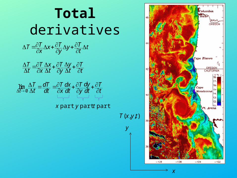
Total derivatives

x

y

( , , )T x y t

TTT x y tx y t

T

yT T xt t tx y t

T T

0limt

dyT dT T dxt dt x dt

T Ty dt t

x part y part t part

The material derivative:derivative “following the motion”

x

y

0limt

dyT dT T dxt dt x dt

T Ty dt t

x part y part t part

,

,

=

velocity of point where measurements are made (boat).

Suppose we kill the engine and drift with the surface

current?

Then current

current; current;

dydxdt dt

dydxdt dt

dydx u zonal v meridionaldt dt

uv

DT Tu vDt t y

Tx

T

Multivariate Calculus 2:

partial integrationseparation of variables

Fourier methods

x

y

( , )T x y

Partial differential equationsAlgebraic equation: involves functions; solutions are numbers.

Ordinary differential equation (ODE): involves total derivatives; solutions are univariate functions.

Partial differential equation (PDE): involves partial derivatives; solutions are multivariate functions.

Notation

2 3

2 2

subscript notatio

"di" = partial der

n:

; ;

iv

,

ative

x tt xttf f ff f fx t x t

Classification

2

2

2

3  0 linear

3  0 nonlinear

3  0 homogeneous

3 1  nonhomogeneous

xxt

x t

x t

x t

f f f

f f f

f f f

f f f

If ( , ) and ( , ) are solutions of a PDE, then any ( ,

Superposition:

linear, homogeneouslinear combinati ) ( , ),

where andon

al are

so con

a sstants,

is .olution

f x t g x taf x t bg x t

a b

Order

2

 0 1st order

3  0 3rd orderx t

xxx t

f f g

f f f

=order of highest derivative with respect to any variable.

Partial integration

21( ,

. .

) )

,

(

( )

2

x

f x y

e g

f x y x

x c y

Instead of constant,add function of other variable(s)

Partial integration

2

2

boundary condition

(0, ) 1

(0, ) 0 ( ) 1

add :

( , ) ;

1( , ) ( )2

1complete solution: ( , 12

( ) 1

)

x f y y

f y c y y

c

f x y x c y

f x y x

f y x

y

y y

x

x

y ( , )f x y

Partial integration

( , ) ( )

beca

. .

(

s

)

u e

,x

f x y c y

yd

e g

f x y y

x

dx x

y

x y y

Partial integration

( , ) ( )

because

Now suppose the boundary condition ( ,

.

) 1

(1, ) ( ) 1

.

( , )

( ) 1

( , 1

s

)

1i

x

f y y

f y y c y y

c y

f x y x

e g

f x y y

f x y c y

ydx y dx y x

xy

y

Partial integration. .

( , ) 0

0 means ( , ) does n

(

o

, )

t actually dep

(

end on

)

.

x

x

e g

f x y

f

f x y c

f y

y

x x

Solution by separation of variables

Try to reduce PDE to two (or more) ODEs.

Is it possible for functions of two different variables to be equal?

( ) ( ) ?f x g y

Is it possible for functions of two different variables to be equal?

Assume ( ) ( )

: ( ) ( ).x x

f x g y

f x g yx

Is it possible for functions of two different variables to be equal?

Assume ( ) ( )

: ( ) ( ) 0

: ( ) 0 (0)

( ) ; ( ) .

x x

y y

f x g y

f x g yx

f x gy

f x c g y c

The PlanManipulate PDE into the form ( ) ( ).

Result is 2 ODES: ( ) ; ( ) .

f x g y

f x c g y c

Example 1

Try ( , ) ( ) ( )

0x yy

f x y X x Y y

f f

Example 1

Try ( , ) ( ) ( )

Substitute: ( ) ( ) ( ) ( ) 0

( ) ( ) ( ) ( )Divide by : 0

( ) ( )

( )( )Rearrange: 0( ) ( )

0

x yy

x yy

yyx

x yy

f x y X x Y y

X x Y y X x Y y

X x Y y X x Y yXY

X x Y y

Y yX xX x Y y

f f

Example 1

Try ( , ) ( ) ( )

Substitute: ( ) ( ) ( ) ( ) 0

( ) ( ) ( ) ( )Divide by : 0

( ) ( )

( )( )Rearrange: 0( ) ( )

( )( ) Viola!( ) ( )

0

x yy

x yy

yyx

yyx

x yy

f x y X x Y y

X x Y y X x Y y

X x Y y X x Y yXY

X x Y y

Y yX xX x Y y

Y yX x cX x Y y

f f

Example 1

( )( )( ) ( )

; , 2 ODEs

; sin( ), cos( )

( , ) ( ) ( ) sin( ) (or something like that)

yyx

x yy

Cx

Cx

Y yX x cX x Y y

X cX Y cY

X e Y cy cy

f x y X x Y y e cy

Thermal diffusion in a 1D bar

0( ,0) ( )T x T x

0x x L( , ) ; xxtTT T x t T

(0, ) 0 ; ( , ) 0T t T L t Boundary conditions:

Initial condition:

Applications

Diffusion of:

• Heat• Salt• Chemicals, e.g. O2, CO2, pollutants• Critters, e.g. phytoplankton• Diseases• Galactic civilizations• Money (negative diffusion)

Thermal diffusion in a 1D bar

0( ,0) ( )T x T x

0x x L( , ) ; xxtTT T x t T

(0, ) 0 ; ( , ) 0T t T L t Boundary conditions:

Initial condition:

Solution by separation of variables

Try ( , ) ( ) ( )

Substitute: ( ) ( ) ( ) ( )

( ) ( )Divide by : c( ) ( )

( ) ( ) ; ( ) ( )

xxt

xxt

t xx

xxtt

T T

T x t X x t

X x t X x t

t X xXt X x

ct c t X x X x

First try

2

22 2

;

Assume 0, or ;

boundary co

 ;

( )

( ) ) 0?

NO GOO

nditions: (0) 0

) 2 sinh(

2 sinh(

0, or D! Try

x

a ax xa t

a ax x

xtt

xxtt

cc X X

ac c a a X X

X A B B A

e X Ae Be

aX A e e x

aX L

c

L

A

A

c

2a

sinh( )2

x xe ex

Second try

2

22 2

 ; sin( ) cos( )

sin( )

( ) sin( ) 0?

NO PROBLEM! , 0,

;

Assume 0, or ;

boundary conditions:

1, 2,

(0) 0

xxt

x

t

x

a

t

a a

cc X X

ac c a a X

e X A x B x

aX A

X

X B

x

aX L A L

a L n n

2

, 2

sin( )

, or

sin ; 1,2,3,

and

( , ) ( ) ( ) sin

a t

n tL

aX A x

a a nL nL

xX A n nL

ne aL

xT x t X x t A n eL

2

( , ) ( ) ( ) sinn tLxT x t X x t A n e

L

Characteristics of time dependence:

•T 0 as t ∞ , i.e. temperature equalizes to the temperature of the endpoints.

•Higher (diffusivity) leads to faster diffusion.

•Higher n (faster spatial variation) leads to faster diffusion.

In fact:

22

2So diffusion time

"Wavelength"

.

n

ntn

L

n

t

Ln

e e

Time scale is proportional to (length scale)2.

In fact:

22

2So diffusion time

"Wavelength"

.

n

ntn

L

n

t

Ln

e e

E.G. Water 1/2 as deep takes 1/4 as long to boil!

Sharp gradients diffuse rapidly.

This observation is surprising.

Now what about the initial condition?

0( ,0) ( )T x T x

0x x LxxtT T

(0, ) 0 ; ( , ) 0T t T L t Boundary conditions:

Initial condition: ?

2

( , ) sinn tLxT x t A n e

L

0( ,0) ( )T x T xInitial condition: ?

2

.

2

0Suppose

( , ) sin

( ,0) sin

( ) sin

Choose , 1 so ( , ) sin

n tL

tL

xT x t A n eL

xT x A

xT

nL

xT x t eL

xL

A n

0x x L

0T

T

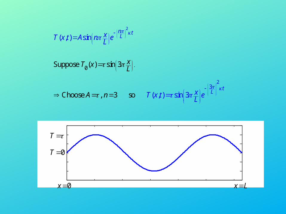
2

.

23

0Suppose ( ) sin 3

Choose , 3

( , ) sin

so ( , ) si 3 n

n tL

tL

xT xL

A n

xT x t A n eL

xT x t eL

0x x L

0T

T

01Suppose ( ) sin sin 3 ?2

x xT xL L

0x x L

22

2

0

3

1Suppose ( ) sin sin 3 ?2

!

and are solusin sin 3

Asin

If tions,

h

T en

tt LL

L

x xe eL L

x

x xT xL L

SUPERPOSITION

eL

2

22

3

3

sin 3

1(

is a sol

, ) sin s

ution.

1Choose 1, in 3 22

tt L

tt LL

xB eL

x xT x t e eA BL L

0x x L

Fourier’s Theorem

0x x L

0 0

1

0

0

ANY FUNCTION ( ) that obeys the boundary conditions (0) 0 and ( ) 0

can be represented as a Fo

( ) s

urier series:

The corresponding solution for the diff

in

u

nn

xT x A n

x T L

L

T T

2

1 (

sion probl

, ) s

em :

n

is

in tL

nn

xT x t A n eL

To find the constants:

002 ( )sin

Ln n

LxA T x dxL

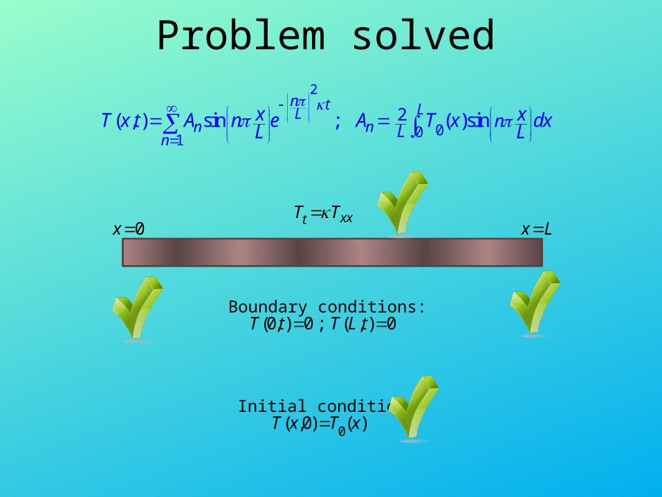
Problem solved

0( ,0) ( )T x T x

0x x LxxtT T

(0, ) 0 ; ( , ) 0T t T L t Boundary conditions:

Initial condition:

2

001

2 ( , ) sin ; ( )si n n t LL

n nn

nL

x xT x t A n e A T x dxL L

Homework clarification3.3 partial integration3.4 separation of variables3.5 Fourier series solution for guitar string

1. Solve for a single Fourier mode• Separate• Choose sign of separation constant • Satisfy boundary conditions and initial condition ht=0 • Write down the general solution satisfying h(x,0)=h0(x), but don’t derive the coefficients for the Fourier series.

2. Interpret• Time dependence: exponential or …?• Describe in physical terms.

3. Time scale• Is the time scale for a mode proportional to the length scale squared? • If not, what?

0x x L

0( ,0) ( )h x h xh

( ,0) 0th x

Isocontours

x

y

( , )T x y

0

/ isocontour slope/

TT x yx y

Ty xy x

y T xx T y

T

T