Biofuel Economics in a Setting of Multiple Objectives

& Unintended Consequences

William K. Jaeger and Thorsten M. Egelkraut Department of Agricultural and Resource Economics

Oregon State University

ABSTRACT This paper examines biofuels from an economic perspective and evaluates the merits of promoting biofuel production in the context of the policies’ multiple objectives, life-cycle implications, pecuniary externalities, and other unintended consequences. The policy goals most often cited are to reduce fossil fuel use and to lower greenhouse gas emissions. But the presence of multiple objectives and various indirect effects complicates normative evaluation. To address some of these complicating factors, we look at a several combinations of policy alternatives that achieve the same set of incremental gains along the two primary targeted policy dimensions, making it possible to compare the costs and cost-effectiveness of each combination of policies. For example, when this approach is applied to U.S.-produced biofuels, they are found to be 14 to 31 times as costly as alternatives like raising the gas tax or promoting energy efficiency improvements. The analysis also finds the scale of the potential contributions of biofuels to be extremely small in both the U.S. and EU. Mandated U.S. corn ethanol production for 2025 reduces U.S. petroleum input use by 1.75%, and would have negligible net effects on CO2 emissions; and although EU imports of Brazilian ethanol may look better given the high costs of other alternatives, this option is equivalent, at most, to a 1.20% reduction in EU gasoline consumption. JEL Classification: Q42, Q48, Q54 Key words: biofuel, biodiesel, cost-effectiveness, indirect land use change effects, net energy, multiple objectives, ethanol, GHG Corresponding author: Jaeger wjaeger@oregonstate.edu

Citation: Jaeger W.K. and T.M. Egelkraut, 2011. Biofuel economics in a setting of multiple objectives and unintended consequences. Renewable and Sustainable Energy Reviews. 15(9): 4320-4333.

1

I. Introduction

The belief that biofuels can reduce dependency on fossil fuels and mitigate climate

change has led many governments to promote their production and use as substitutes for gasoline

and petroleum-based diesel, using mandates and subsidies. With the added suggestion that

biofuel production could encourage rural economic development and poverty alleviation, biofuel

subsidies in 2006 amounted to $11 billion ($11x109) in the leading OECD producing countries

(Global Subsidies Initiative 2007). The largest biofuel programs are in the U.S., the EU, and

Brazil, but many developing countries are also implementing or considering similar policies to

encourage domestic biofuel production.

Renewable energy promotion has become a policy priority in many countries, and

biofuels are one type of renewable energy. However, as with other renewable energy options, the

emergence of biofuel promotion has not been based on, or preceded by, a detailed analysis of its

prospects, implications, and the potential for achieving their intended objectives (Heal 2010) and

hence may allocate billions of tax-payers dollars inefficiently. The picture is further clouded by

the fact that biofuels constitute an indirect means to achieve their central goals, so that the

connections between increased biofuel production and the resultant reductions in both fossil fuel

use and greenhouse gas (GHG) emissions are far from obvious. Moreover, these efforts may

cause externalities in the form of feedback effects and other unintended consequences, both

pecuniary and non-pecuniary, that impose additional costs on society. The general theory of

second-best (Lipsey and Lancaster 1956) warns us that government interventions to correct

market failure may actually reduce welfare because other optimality conditions do not hold. This

2

possibility becomes particularly important when considering a) the direct and indirect ways in

which large-scale biofuel production alters existing uses of energy and land and b) other impacts

via pecuniary and non-pecuniary externalities.

Indeed, only recently has attention been drawn to some of the effects of biofuels on food

prices, energy use, land-use change and carbon emissions. Given both the lacking transparency

and emerging evidence of these effects, it is important to examine what we now know and to

illuminate this information in ways that will inform good policy decisions. The two main

questions policy makers need to have answered in relation to the central policy goals are: a) How

do the costs of biofuels compare to other options? and b) Can biofuels be made available on a

large enough scale to make significant progress toward those goals?

This paper’s aim is to investigate these two critical questions. Since biofuels and

alternative interventions affect both the use of fossil fuels and GHG emissions to different

extents, we first develop an explicit cost-effectiveness measure to compare options in equivalent

terms, i.e. for the same set of primary outcomes. With this measure the relative costs of various

policy alternatives can then be directly assessed in relation to the policies’ multiple ends or goals.

This is an important distinction from prior research that commonly ignores biofuel policies’

complexity by focusing on only a single policy dimension or that assumes simple gallon for

gallon fuel substitution without considering the multitude of associate effects. Finally, we

examine the potential scope of biofuels’ contribution toward their stated policy objectives.

There are some important technical and engineering aspects of biofuels that, because of

their complexity, warrant some attention before developing our framework for evaluating the

two questions posed. In sections II and III, summaries of background information and key issues

are presented to provide important context (although less technical inclined readers may skip

3

sections II and III). Section IV develops a framework for estimating the cost-effectiveness of

biofuels in comparison to other policy options and is followed in section V by a presentation of

the data and estimations undertaken for each option. The results are described in section VI, and

section VII offers some concluding thoughts.

II. Background

Although biofuel promotion has accelerated over the past decade, production and use of

ethanol as a transportation fuel has been supported in the U.S. since 1978 and in Brazil since the

1930s. Europe’s experience with biofuels is more recent. Among renewable energy options,

biofuels have attracted attention in part because they are liquid fuels that can be easily used in

motor vehicles, and in some cases with little or no modification of existing gasoline or diesel fuel

engines.

In the U.S., federal and state ethanol programs were initially aimed at supporting farm

prices and farm incomes. Later the rationale for these programs shifted to environmental quality,

and more recently to energy security/independence and reduced GHG emissions (Tyner 2007).

Federal subsidies have ranged from $0.40 to $0.60/gallon and are currently at $0.45. When state

programs and subsidies for start-up and investments are included, the total subsidy in 2006 is

estimated to range from $1.05 to $1.38/gallon (Koplow 2006). Federal legislation has, in the past

decade, established a schedule of renewable fuel production targets, the most recent being the

Energy Independence and Security Act of 2007 which sets targets for renewable fuels

consumption (rising from 9 billion gallons in 2008 to 36 billion gallons in 2022). The volumetric

requirements by renewable fuel type were adjusted in 2010 under the revised Renewable Fuels

4

Standard (RFS2). The total mandate of 36 billion gallon by 2022 requires cellulosic ethanol

production to rise from 0.1 billion gallons in 2010 to 16 billion gal, corn ethanol production to

rise to 15 billion gal, and an additional 5 billion gallons of non-cellulosic “advanced” biofuels

including a minimum of 1 billion gallons of biodiesel (primarily soybean-based).1

Ethanol production for sugarcane in Brazil dates back to the 1930s. The Brazilian

government began in 1975 a “pro-alcohol” program to produce ethanol from cane biomass using

quotas, fixed prices, and subsidized loans (Martines-Filho et al. 2006). Between 1997 and 1999,

sugar and ethanol prices were deregulated and flex-fuel vehicles introduced so that consumers

could choose their desired fuel mix (all gasoline in Brazil is blended with 20-25% ethanol).

National production in 2008 was 6.5 billion gallons, exceeded only since 2006 by the U.S.

U.S. current

corn ethanol capacity is approximately 13 billion gallons including idled capacity.

Europe’s experience with biofuels started in the 1990s when several countries started

producing biofuels in response to concerns about energy security. Beginning in 2000, the EU

saw a number of renewable energy proposals put forward. A biofuel target for 2% of

transportation fuel by 2005 and 5.75% by 2010 was established in 2003, only to be abandoned in

2005 when it became clear that production would fall 1.4% short of the 2% target. In 2006, the

EU replaced quantitative targets with a strategy aimed at continued promotion of biofuels in the

EU and developing countries, support for research into second-generation biofuels such as

cellulosic ethanol and exploration of opportunities for developing countries to produce biofuel

feedstocks and biofuels (Van Thuijl and Deurwaarder, 2006). In 2009, a new EU mandate was

established that calls for 10% biofuel content in transportation fuels by 2020.

1 Cellulosic ethanol is derived from lignocelluloses materials in wood, grass, corn stover, or other non-edible parts of plants. Non-cellulosic advanced biofuels include biodiesel derived from algae.

5

III. Issues Affecting Biofuels’ Potential

Biofuels were initially seen as an easy solution to energy and environmental problems

because they represented energy grown by farmers and captured from the sun that would be

carbon neutral because the CO2 emitted when burning the biofuel was simply the release of CO2

previously absorbed from the atmosphere by the plants grown as feedstock. In this “win-win”

view, a clean, renewable energy in liquid form (so it could be used as a transportation fuel) could

be grown domestically to reduced dependency on fossil fuels, save foreign exchange, create jobs,

and protect the environment. By now we understand, however, that the biofuel picture is more

complex given the resources required to produce feedstocks in large quantities, as well as the

externalities and indirect market effects (pecuniary externalities) caused by large-scale

production of biofuels.

These considerations can be organized under three topics: life-cycle analysis, pecuniary

externalities, and non-pecuniary externalities. First, life-cycle analysis (LCA) for biofuel

production reveals that both energy and GHG accounting involve the use of fossil fuels, which in

turn imply GHG emissions unrelated and in addition to the CO2 absorbed by immediate plant

growth. Second, large scale biofuel production generates pecuniary externalities that raise

concerns about food prices and cause changes in land use. While these market effects may

represent negative externalities narrowly defined, to the extent that food security and

distributional effects are part of concern, these pecuniary effects deserve attention. Third, direct

and indirect externalities raise additional issues related to land use, carbon emissions, water

scarcity, and air pollution. These aspects of biofuel policies potentially lead to revisions in their

expected energy and climate change gains, and in doing so alter significantly our understanding

6

of biofuels’ costs as well as the scale of biofuels’ possible contribution toward the stated

program goals.

Life Cycle Analysis of Biofuels

The perception that consuming a gallon of ethanol eliminates the use of a gallon of

gasoline is misleading for at least two reasons. First, ethanol contains less energy per gallon than

gasoline. And second, because fossil fuels are used in the production of biofuels and their

feedstocks, the overall net contribution of biofuels to energy availability requires deducting the

input energy used in the production process from the gross energy content of the biofuel. Life

Cycle Analysis (LCA) looks at the entire process of producing and combining inputs including

transportation to the final place of consumption. LCAis often used for energy accounting, but it

can also be applied to fully account for carbon emissions, water use, or other materials, yielding

a measure of the net energy or net materials use. In the case of biofuels, the solar energy

contained in the feedstock is considered “free”, and is therefore ignored. . As a result, biofuel

production creates an energy gain rather than an energy loss – but the gain will be less than the

amount of energy in the fuel.

Given the objectives of reducing fossil fuel use and GHG emissions, LCA permits

evaluation of the net contribution of biofuels. There are several ways to express the relationship

between fossil fuel energy inputs used to produce biofuels and the energy contained in the fuel

itself. The ratio of fossil fuel inputs to energy in fuel provides a succinct indicator. For fossil

fuels themselves, of course, this ratio will be greater than one since some fossil fuel is needed to

extract, transport and refine gasoline from crude oil. Central estimates of those ratios are 1.23 for

gasoline and 1.15 for petroleum diesel. For biofuels, these ratios vary considerably across fuels,

7

reflecting a wide range in net energy contributions, the most cited values being 0.66 for corn

ethanol, 0.38 for soy biodiesel, and 0.08 for cellulosic ethanol.

Because biofuels are produced using fossil fuel inputs (including nitrogen fertilizer for

corn production), they are not carbon neutral. Similar to the LCA energy accounting life-cycle

carbon emissions can also be evaluated for biofuels. Carbon LCA depends greatly on technology

and types of fossil fuel used. Central estimates for corn ethanol suggest a 20% reduction in CO2

emissions per MBTU (million British Thermal Units) when substituting for gasoline. The

reduction is 40% for biodiesel in the U.S. and Europe, and 78% for Brazilian sugarcane ethanol

(U.S. EPA 2006).

LCA provides a useful first indication of the energy or GHG consequences of using

biofuels. But because it does not account for behavioral responses or market effects, LCA can be

a poor indicator of the general equilibrium effects of introducing biofuels and overstate their

benefits. Discussed below are the potential pecuniary externalities occurring in product and input

markets due to biofuel production, as well as the consequent externalities which occur through

these indirect changes and affect both energy and GHGs.

Pecuniary Externalities and Food Prices

Biofuel production and consumption creates pecuniary externalities by shifting supply

and demand in input and output markets. How these effects play out, however, will depend on

the kind of policy used to promote biofuel consumption, and to what extent the costs of biofuels

are born by consumers. Biofuel production and consumption can be promoted with subsidies,

regulatory requirements, or other instruments. Except where noted, the analysis below assumes

8

that biofuels are subsidized at a rate that matches the cost per BTU for gasoline (or petroleum

diesel in the case of biodiesel).

When consumers switch to biofuels the demand for gasoline will decrease leading to a

decline in gasoline prices. Lower gasoline prices, however, will increase the quantity of gasoline

demanded so that the net decrease in gasoline consumption (and associated fossil fuel inputs and

CO2 emissions) can be expected to be less than the increase in biofuel consumption. This second-

order effect may be offset to the extent that biofuel mandates (like the 10% requirement for

gasoline in the U.S.) raise gasoline costs when the more costly biofuels are blended with

gasoline. It is difficult to estimate which effect dominates at any given point in time, but the net

result will be marginal at best and can therefore be quantitatively ignored. The subsequent

analysis, thus assumes a BTU-for-BTU substitution from petroleum fuel to biofuel.

Co-products in biofuel production including distiller dry grains (corn ethanol) and

soybean meal are marketable as a component in livestock feed, and so these products are likely

to displace existing animal feed production. Because the displaced animal feed production would

have required energy to produce comparable energy-laden feed rations, an energy “credit” is

generally assigned in the biofuel energy accounting (outside of LCA). This “credit” recognizes

this substitution effect that “saves” energy at the level of the economy even though it does not

occur within the standard LCA boundaries. In the analysis below co-product energy credits are

included.

Biofuel feedstock production requires large areas of agricultural land. Drawing land into

the biofuels market, therefore reduces the supply of land for food, feed and other agricultural

production. This shift puts upward pressure on land prices but, more importantly, reduces the

supply of food and feed. This leftward shift in the food supply schedule leads to two very

9

important effects: a) an increase in food prices, and b) an expansion of agricultural production in

other areas not previously under cultivation.

Beginning in 2006, world food prices rose dramatically into 2008, with prices for corn

and other staple foods such as rice, soybeans and wheat doubling. The increases caused protests

and political unrest in many parts of the world, with biofuels taking much of the blame.

Numerous studies have since attempted to assess the causal factors leading to these sharp

increases in worldwide food prices. In general they agree that multiple factors contributed: rapid

economic growth in some developing countries leading to increased demand; weather and crop

disease shocks in 2006-07, devaluation of the U.S. dollar, and growth in the production of

biofuels (Abbott et al. 2008). Most studies also concluded that biofuel policies were a significant

factor, with estimates of the share of food price increases attributable to biofuel policies ranging

from 10% (USDA 2008) to 75% (Mitchell 2008). Using a multi-market analysis, Rajagopal et al.

(2009), for example, conclude that about one-quarter of food price inflation in 2007-08 was due

to biofuels. The connection between biofuels and increasing food prices drew worldwide

attention to the potential adverse pecuniary effect of biofuel promotion and has been a significant

factor in the decline in public support for biofuel policies in many countries.

Externalities, Indirect Land Use Change

The effects of supply or demand shifts tend to be viewed neutrally in economics as

pecuniary externalities, but not as inefficient. Indeed, such pecuniary externalities may represent

welfare improvements if they arise as a result of interventions to correct market failures. In the

presence of other market failures, however, the Theory of Second Best implies that such market

adjustments can be welfare reducing. Food price increases caused by biofuel production are one

10

example of a pecuniary externality that causes food insecurity among the poor and potentially

leads to significant human suffering.

Land markets are also affected. Most biofuels require land-intensive feedstock

production, which increases the demand for (cultivable) land. The resulting incremental increase

in the equilibrium quantity of land under cultivation may occur in a different location than where

the biofuel feedstock is grown. Indeed, if feedstock production displaces food production in one

area, food price adjustments are likely to bring additional land into cultivation elsewhere.

Although this is a standard market adjustment phenomenon, it has become a pivotal and

controversial issue for biofuels because expanding production onto previously uncultivated land

releases significant quantities of carbon that have accumulated over long periods in soil and

vegetation. These indirect external effects from biofuel production can generate carbon

emissions in excess of the emissions reductions promised by substituting biofuels for gasoline

(even when averaged over a 30-year period). Therefore, the magnitude and consequences of

Indirect Land Use Change effects (ILUCs) need to be considered when evaluating biofuels.

Estimates of the magnitude of ILUCs were first presented by Searchinger et al. (2007),

who included both the reduced emissions from substituting biofuels for gasoline as well as the

increased emissions the ILUC effects. Compared to a simple LCA that showed a reduction of

20% in CO2 emissions for corn ethanol, Searchinger et al.’s inclusion of ILUC effects produced

an estimated increase of 93% in emissions. However, more recent estimates based on revised

global models forecast smaller ILUC effects. In the case of corn ethanol, Tyner et al. (2010)

suggest that the ILUC effects are sufficiently low so that the net effect from corn ethanol

production is a small reduction in CO2 emissions rather than an increase as suggested by

Searchinger et al. (2007). In the case of Brazilian sugarcane ethanol, life-cycle analysis suggests

11

a 75% reduction in GHG emissions, whereas the inclusion of land-use changes produces an

estimated 125% increase compared to gasoline. This large effect in Brazil occurs as sugarcane

displaces rangeland, and rangeland displaces forests and other native habitat (Lapola et al.

2010).2

Jobs and Rural Development

Job creation and rural development are sometimes mentioned by governments as

additional reasons for promoting biofuels. The notion that biofuels could achieve energy

security, environmental goals and at the same time create jobs and stimulate rural economies is

an appealing prospect. There is little evidence, however, that increased biofuel production will

have significant, long-term positive job impacts in rural areas. A typical 100 million gallon

ethanol plant provides an estimated 45 jobs. Ethanol subsidies in the U.S. are currently

$0.45/gallon, the equivalent of $1 million per job per year. Some proponents estimate substantial

indirect job creation, but these projections are based on static, regional input-output models and

do not reflect long-term general equilibrium adjustments including shifts in jobs among regions.

Indeed, one study modeling the effects of U.S. biofuel mandates on shifts in agricultural

production among regions concluded that cellulosic ethanol would expand in the southern states

but that it would not provide any additional economic activity because the increase in ethanol

output would be offset by a reduction in livestock production (Dicks et al., 2009).

2 An alternative approach taken in a recent National Research Council report involves taking account of the direct land use effects (where the biofuel feedstock is grown) and attributes the ILUC effects to the “second product” that is grown on that land (NRC 2010). The ILUC approach, by contrast, involves a “with versus without” analysis to attribute changes associated with a policy promoting biofuels. The latter approach recognizes that the “second product” (i.e., food) has been displaced from one location to another, and any change in its direct land use effects will arise due to that displacement.

12

Policy Choice and Interactions

The particular policies chosen to promote biofuels will affect its effectiveness, its cost,

and also the associated pecuniary externalities and other changes. The net effect of the policies

on fuel prices is one important factor. A blend mandate introduced independent of other policies

may, to the extent that biofuels are more costly than the fossil fuel with which they are blended,

discourage driving and hence lower fossil fuel consumption. The 10% blend requirement for

ethanol in gasoline would have such an effect, were it not for the additional policies that

subsidize production of ethanol. In the U.S. ethanol costs about 40% more to produce than the

cost of gasoline on a BTU basis, and the subsidy per BTU for ethanol is similarly about 40%.

The net effect of combinations of biofuel policies is not always obvious, however. De

Gorter and Just (2009, 2010) demonstrate how mandates, taxes and subsidies for biofuels can

interact with each other, and with other policies, in ways that significantly alter the social costs

and benefits of biofuels. Based on analyses of U.S. corn ethanol production, they find that a

biofuel blend mandate can increase or decrease retail fuel prices depending on the relative supply

elasticities, but that a biofuel tax credit will always result in lower fuel prices, and hence

increased consumption (de Gorter and Just 2009). If tax credits are implemented alongside

biofuel blend mandates, the effect of the tax credit will be to subsidize fuel consumption instead

of biofuels (relative to a mandate with no subsidy), which will have the effect of increasing oil

dependency and CO2 emissions (de Gorter and Just, 2009). Ethanol policies that affect corn

prices can exacerbate the inefficiencies of farm subsidies (and vice versa).

IV. Analytical Framework

13

While the above discussion underlines the great complexity of assessing biofuels, it also

shows that many effects are relatively minor in magnitude. These effects can thus be neglected

without changing the general qualitative conclusions. The following analysis therefore takes

account of only the main factors impacting the two policy goals (reduced fossil fuel use and

reduced GHG emissions), and compares biofuel with other policy options that could also achieve

those goals. Sufficient current information is available to permit a reliable estimate of the net

gains toward these two goals.

Although a standard approach to evaluating different kinds of policies is benefit-cost

analysis, in the context of biofuels, estimating the value of benefits from reduced fossil fuel use

and GHG emissions is complex, uncertain and controversial. A benefit-cost analysis would

therefore undoubtedly raise questions about the validity of the benefit estimates (see, for

example, Banzhaf 2009; Hahn and Cecot 2009) and distract from questions of cost and cost-

effectiveness, which are important by themselves and can be examined independent of the

precise benefit measures.

An alternate approach when the main focus of attention is not the benefits of the outcome,

but rather the costs of alternative ways to achieve those outcomes, is cost-effectiveness analysis.

Cost-effectiveness analysis compares the costs of alternative means for achieving a specific

outcome, and thus identifies the least-cost alternative. It has been successfully used in health

economics (see, for example, Garber and Phelps 1997) and has increasingly been employed by

economists in addressing environmental policy issues. For example, economists have applied

cost-effectiveness to questions of conservation technology adoption (Khanna, Isik and Zilberman

2002), selecting biological reserves (Polasky, Camm and Barber-Yonds 2001), ecosystem

management (Rashford and Adams 2007), and pollution control policies (Burtraw, et al. 2001).

14

Evaluating biofuels in terms of cost-effectiveness for achieving two central goals – reducing

fossil fuel use (both to decrease dependency on petroleum imports and to shift generally toward

renewable energy) and reducing carbon emissions – and also examining their scope for

furthering those objectives complicates the application of cost-effectiveness analysis since

alternative interventions may result in changes that are not directly comparable (e.g., when the

relative gains among the multiple goals occur differently). In the current context, certain

interventions affect both the use of fossil fuels and GHG emissions (e.g., a gas tax or carbon tax),

whereas others address only one objective (e.g., carbon sequestration), and still other

interventions may promote one goal but may adversely affect the other (e.g., biofuels that

substitute for fossil fuels but increase carbon emissions as a result of land use changes). To

evaluate the costs of alternative policies for achieving a common outcome or common

combination of outcomes, an explicit cost-effectiveness measure is developed to compare

options in equivalent terms, i.e. for the same set of primary outcomes.

Thus our analysis evaluates the direct and quantitative relationship between the ends and

means: between the ends of reduced fossil fuel use and reduced GHG emissions, and the means

of biofuel promotion or alternative policies. The analysis evaluates the relative costs of these

alternatives in relation to the policies’ multiple ends or goals -- and this approach distinguishes

our analysis from prior assessments. And finally our study examines the potential scope of the

contribution of biofuels toward those ends.

The relationships between ends and means are easily overlooked if they are not clearly

established. The choice of policy instrument is particularly important because of the way it will

often frame the discussion of the policy’s objectives. This point has been emphasized by

Keohane (2009) in the context of discussing the merits of cap-and-trade versus a carbon tax to

15

address climate change. Keohane argues that cap-and-trade will draw attention to the actual level

of emissions whereas a carbon tax will draw attention to the level of the tax. In the case of

biofuels, by setting policy goals in terms of gallons of ethanol or biodiesel, the debate has

focused in many settings primarily on progress toward meeting those goals, and to a much lesser

extent on the actual reductions in fossil fuel inputs used, the GHG emission reductions, or the

cost of achieving either of these goals. A case in point is the U.S., where a debate has been

underway for several years but, until recently, with little attention to the (biofuel) policies’ actual

effectiveness toward reduced fossil fuel use or lowering GHG emissions, and with no

quantitative appraisal of its cost-effectiveness in achieving either of those two underlying goals.

By focusing directly on these underlying goals and by developing and applying measures of cost-

effectiveness and scope, the analysis presented here evaluates the promotion of biofuels using

metrics that connect ends and means.

Here, each alternative biofuel is considered in terms of its costs, fossil fuel inputs, and

GHG implications relative to the petroleum-based fuel (gasoline or diesel) it is assumed to be

replacing. Biofuels also require land for feedstock production which either directly or indirectly

affects carbon emissions. Moreover, government may implement carbon sequestration actions

such as forest management and afforestation, although below only sequestration via changes in

forest management is considered because it does not require additional lands to be taken out of

alternative uses (such as agriculture). Where biofuels are more costly to produce than petroleum-

based fuels per unit of energy content, the comparisons here will assume that government policy

involves incentives in the form of producer or consumer subsidies at levels necessary to achieve

a desired level of biofuel use. This is a conservative approach that will simplify comparisons

among policy options and at the same time avoid estimating the magnitude of inefficiencies one

16

can expect with regulatory approaches. The only additional cost in this case will be the cost of

public funds required to subsidize biofuels at a level that makes them competitive with

conventional fuels. We further assume that consumers’ utility is unaffected when biofuels are

substituted for fossil fuels; replacing a BTU of fossil fuel energy with a BTU from biofuels

involves no direct welfare change at the consumer level.

The substitution of biofuel for fossil fuel has implications in terms of costs as well as the

social goals on which biofuel programs have been justified. We assume that when consumers

switch from petroleum fuel to biofuel, there is an equal reduction in demand for petroleum fuel

which, via market signals, leads to a reduction in production of petroleum fuels. The net effect of

the substitution comes from an increase in life-cycle energy and GHG implications for the

biofuel and a decrease in the life-cycle energy and GHG implications for the petroleum fuel. The

cost-effectiveness of biofuels in achieving each of these goals is defined as the change in cost

divided by the change in GHG emissions, or as the change in cost divided by the change in fossil

fuel use. These relations are presented explicitly in the Appendix.

The objective is to compare the cost-effectiveness of these alternatives to other

interventions that may be lower cost, such as a gas tax or carbon tax, or with energy efficiency

improvements, or forest carbon sequestration. A gas tax or energy efficiency improvement that

reduces GHG emissions by one metric ton (tons) will at the same time reduce fossil fuel input

use. Some biofuels may further one objective (reduced fossil fuel use) but may have an adverse

effect in terms of GHG emissions due to their land requirements and indirect effects on terrestrial

carbon stores. By contrast, carbon capture and sequestration resulting from changes in forest

management will reduce net carbon emissions but may have no significant effect on fossil fuel

use. Programs that invest in increased energy efficiency or that promote energy conservation are

17

likely to reduce fossil fuel use and greenhouse gas emissions, but in different proportions than

with a gas tax (i.e., since many energy conservation measures will reduce natural gas

consumption and use of electricity, they will have different GHG implications than with gasoline

or diesel fuel). These differences in outcomes related to their different objectives make

comparing cost effectiveness ratios problematic, because the denominators, or measures of

effectiveness, are not equivalent.

This problem has been met in the scientific literature with a number of suggested

approaches for multiple-objective or multi-criteria decision analysis (see, for example, Nijkamp

and Rietveld 1987). One approach that allows evaluation of cost-effectiveness without assigning

weights to different objectives involves comparing interventions, either individually or as

combinations, that achieve identical outcomes for all objectives. Depending on the composition

of the various alternatives (sets), this approach may offer similar insights about relative costs as

in the case of individual actions addressing individual objectives. For any given action such as

raising the gas tax, it will generally be possible to find a combination of other actions (e.g.,

biofuel production plus forest carbon sequestration), that attains the same outcomes (in terms of

reduced GHG emissions and reduced fossil fuel use) as the gas tax. For each such action or

combination of actions, we can thus compare their cost-effectiveness measures directly. See the

Appendix for additional details.

To illustrate this approach, consider a gas tax increase that reduces gas consumption by

100 gallons of gasoline (Figure 0). This reduction translates into a decrease in fossil fuel inputs

of 14.8 MBTU, but also a decrease in GHG emissions of 1.17 tons CO2-e (CO2-equivalent).3

3 A gallon of gasoline is assumed to contain 0.120 MBTU of energy, require 0.148 MBTUs of fossil fuel energy to produce, and generate 97,000 grams of CO2-e per MBTU of energy in fuel.

How can these same results be achieved by producing biofuels rather than by raising the gas tax?

18

This same change in fossil fuel input use (-14.8 MBTU) could be attained by producing 157

gallons of corn ethanol. However, producing this amount of corn ethanol is estimated to reduce

net GHG emissions only negligibly by 0.10 tons CO2-e when ILUC effects are included

(discussed below). Although the outcomes for a gas tax increase and for production of 157 gal of

corn ethanol are identical in terms of their effects on fossil fuel input use, their effects on GHG

emissions are quite different. However, a third intervention, carbon sequestration based on

changes in forest management, represents an alternative or independent policy action that, if

combined in this case with the production of corn ethanol, could give rise to reductions in GHG

emissions overall. Specifically, if the production of 157 gallons of corn ethanol is complemented

by a particular amount of forest carbon sequestration, the combination of these two actions could

achieve exactly the same outcomes as the gas tax.4

To summarize, if the production of 157 gal of

corn ethanol is combined with 1.07 tons (CO2-e) of forest carbon sequestration, the combined

effect would be reductions in both fossil fuel input use (14.8 MBTU) and carbon emissions (-

1.17 tons), and be exactly identical to the those due to the 100 gallons reduction in gasoline use

achieved with the gas tax increase. Thus, with identical outcomes (as summarized in below), and

with costs computed in comparable ways, these two different options (a gas tax on the one hand,

versus a combination of corn ethanol production and forest carbon sequestration on the other

hand) can be compared in a cost-effectiveness framework.

4 Forest sequestration can involve an increase the density of biomass in forests (forest management) or it can involve expansion of forest area (afforestation) (Newell and Stavins 2000). We assume here that forest carbon sequestration is achieved via changes in forest management and does not displace agriculture.

19

Figure 1. Hypothetical effects of specific increases in the gas tax, corn ethanol production, and

forest carbon sequestration on fossil fuel use and greenhouse gas (GHG) emissions.

V. Data and estimation

The above approach is applied to each of the main biofuels produced or mandated (corn

ethanol, soybean biodiesel, and cellulosic ethanol from switchgrass in the U.S., and

rapeseed/canola biodiesel in the EU). Sugarcane ethanol produced in Brazil and exported to the

U.S. or EU is also evaluated as an alternative to domestically-produced biofuels. These biofuels

represent the vast majority of current biofuel production and production mandates worldwide.

Estimates of the energy implications of a biofuel policy are based on LCA for the energy

inputs utilized to produce, process, and transport biofuels and conventional fuels and the energy

contained in the fuel. A similar life-cycle framework is used to estimate the GHG effects. Certain

market effects are represented at least implicitly (e.g., Hill et al. 2007) in these LCAs. For

20

example, biofuel energy accounting typically includes assigning an energy credit for the co-

products generated during feedstock processing (e.g., distiller dry grains, oilseed meal), as these

are generally sold as livestock feed rations. The implicit assumption justifying this energy credit

is that market adjustments, or indirect effects in the animal feed market due to the addition of

biofuel co-products, will lower the production of animal feed from other sources which in turn

will reduce the energy used in traditional animal feed production. Indeed, the market-induced

effect underlying the rationale for a co-product energy credit is similar to the indirect land use

effect for GHG emissions: production of biofuels has effects in other markets and those market

implications for energy and GHGs should be taken into account when evaluating the general-

equilibrium effects of biofuel policies.

Central estimates for the key technical and economic parameters including production

and processing costs, life-cycle fossil fuel energy, and life-cycle GHG effects are summarized in

Table 1(see appendix for additional details). In general, biofuel cost estimates are based on

market prices and for those alternatives not yet commercially available (e.g., cellulosic ethanol)

on peer-reviewed studies. Assumptions regarding technical parameters for energy and GHG

accounting as well as ILUC effects are drawn from the growing scientific literature and from

government studies (see appendix for details).

In addition to the biofuels being evaluated, three alternative interventions are assessed for

comparison purposes: gas tax increases, forest carbon sequestration, and energy efficiency

improvements. Each is discussed below.

A. Gas tax

21

The cost of using a tax to reduce gasoline consumption and its associated GHG emissions is

analyzed in the literature. A range of studies have estimated the long-run own-price elasticities of

gasoline demand in the U.S. West and Williams’ (2007) estimates center around -0.51; Parry and

Small (2005) conclude that the best consensus long-run elasticity is -0.55. An earlier meta-

analysis found a median value of -0.43 (Espey 1998). Similar elasticities lead West and Williams

(2005) to conclude that the initial marginal cost of a gas tax increase that results in one less

gallon of gasoline consumed is $0.26/gallon (based on prices and U.S. gas taxes in 1997). Their

estimate takes account of the long-run responsiveness in miles-per-gallon to gas price, and also

the complementarity between gasoline consumption and leisure and hence the effects on the

costs of public funds. When applied to current taxes and prices, and using the Parry and Small

“consensus” elasticity estimate of -0.55, these values produce cost estimates of $1.46/MBTU for

reducing fossil fuel use and of $18.60/ton for GHG reductions.5

For the EU, the estimated responsiveness of gasoline consumption to the gas tax is based on

a central demand elasticity estimate of -0.75 (Graham and Glaister 2002). This differential

between the U.S. and European own-price gasoline demand elasticities is consistent with Espey’s

(1998) meta-analysis. When the West and Williams marginal cost relationship is adjusted to

reflect EU gasoline prices, taxes, and the own-price gasoline demand elasticity, the results

indicate that an additional 1% reduction in EU gasoline consumption requires an increase in the

gas tax of $0.065/gallon, the marginal cost of which is $2.76/gallon. The EU costs to reduce

fossil fuel use and GHG emissions with a gas tax are then $18.60/MBTU and $237/ton of GHGs,

which in both cases is more than 12 times as costly as in the U.S. The marginal costs associated

5 The marginal cost relation in West and Williams (2005) is based on a gas price of $1.19, gas tax of 0.367, a marginal cost of funds of 1.02, and own-price elasticity of demand for gasoline of 0.46. The reduction in fossil fuel input energy per gallon of gasoline avoided is 0.148 MBTU, and the reductions in GHG emissions amount to 0.097 tons per MBTU of gasoline.

22

with increasing the gas tax are greater in the EU primarily because gasoline taxes are already

considerably higher there than in the U.S., increasing the distortionary costs to a larger extent.

B. Forest carbon sequestration

Carbon sinks are often viewed as a potentially low-cost offsets to GHG emissions and an

alternative to reduced fossil fuel use or fuel switching. Carbon sequestration alternatives include

increasing soil carbon in agricultural lands, and also carbon capture and storage for which carbon

would be sealed in abandoned oil and gas wells or injected into other geologic features. Current

evidence suggests, however, that forest sequestration may be lower cost than other alternatives.

Forest carbon sequestration options are recognized under the Kyoto Protocol, although issues of

monitoring and leakage have given rise to uncertainty and confusion about implementation.

Nevertheless, there are now many studies that have evaluated the potential as well as the costs of

forest carbon sequestration either by afforestation (increasing forested areas) or forest

management (managing existing forests in ways that will increase the amount of sequestered

carbon with, for example, lengthened rotations; for more detail see van Kooten and Sohngen

(2007) as well as Stavins and Richards (2005)).

The current analysis focuses on employing carbon sequestration options that, unlike biofuels,

do not displace food production and so are unlikely to involve significant adverse ILUC effects.

These non-food-displacing options may however not always be the lowest cost alternatives.

Richards and Stokes point to “conservative estimates” by Stavins (1999) of costs around $33/t

CO2-e for these options. Moreover, there are also questions about implementation, leakage and

additionality that argue for erring on the conservative side. Therefore, this study adopts Stavins’s

(1999) $33/t CO2-e as the baseline cost estimate for the U.S. For the EU, a cost of $118/t CO2-e,

23

is assumed based on estimates that carbon sequestering forest management approaches are 3.6

times as costly in Europe (van Kooten and Sohngen 2007). Importantly, these costs do not

assume that changes are achieved via subsidies, and hence the costs of public funds are not

included. A regulatory approach or combination of taxes and subsidies could presumably achieve

increased carbon sequestration with a net fiscal cost.

C. Energy efficiency improvements

Numerous studies address the potential, obstacles, and cost of improved energy efficiency in

industry, buildings, and residential uses (e.g., Jaffe and Stavins 1994). Recent analyses of

mitigation options for GHG include energy savings investments in transportation sectors, but

also in energy supply, buildings and industry (IPCC 2007, chapter 11, Table 11.3). A recent

study of the potential for low-cost energy efficiency improvements in the U.S. by the McKinsey

Company (Granade et al. 2009) finds that energy efficiency offers a large, low-cost energy

resource, but that significant hurdles need to be overcome, primarily at the policy level. The

McKinsey study concludes that interventions to encourage energy efficiency gains could yield a

recurring contribution equivalent to more than 9 quadrillion BTUs (9x1015) per year, or roughly

23% of projected total annual U.S. energy demand, which at the same time would lower annual

GHG emissions by more than 1 Gt (gigaton). The IPCC (2007) analysis projects more than 10 Gt

potential annually for GHG mitigation globally through energy savings from energy supply,

buildings and industry (IPCC 2007, Table 11.3), a value that is broadly consistent with the

McKinsey and other studies. The estimates from Granade et al. (2009) are used here to

characterize a non-transport alternative energy policy to reduce fossil fuel energy use and GHG

emissions for the U.S. All potential positive net present value energy efficiency improvements

24

represent a total level of annual energy use reductions that is equivalent to a 40% reduction in

gasoline consumption. These energy efficiency improvements are estimated be possible from a

wide range of actions including information and education, incentives and financing, changes in

codes and standards that could eliminate significant barriers to energy efficient practices and

technologies.

VI. Results

A useful starting point is to make some straightforward observations. There are

significant differences in the cost of production among biofuels and also in the energy content

per gallon of fuel (Table 1). The amounts of fossil fuel energy inputs required per MBTU of

energy-in-fuel, however, vary even more (from 0.04 to 0.66 per MBTU) due to the large

differences in input energy required to produce some biofuels. When biofuel costs are measured

per unit of reduction in the use of fossil fuel inputs, these cost relationships also vary widely

among biofuels and between biofuels and options such as a gas tax or energy efficiency

improvements. Similarly, large differences emerge when costs are represented for reducing GHG

emissions, including “infinite costs” for those cases where GHG are estimated to increase. These

simple cost measures, however, relate the costs of each option to incremental changes for only

one policy objective at a time, and therefore may provide a misleading basis for comparison

when multiple objectives are at issue.

A. Costs and scale of individual alternatives

25

To visualize the underlying differences among biofuels and other possible policy

alternatives, our results are first presented as simple two-dimensional vectors (Figure 1). Each

dimension represents one of the two policy objectives - reduction in fossil fuel use and reduction

in GHG emissions. For purposes of comparison, each vector is chosen to reflect the reductions

achievable at a cost of $1 billion. The results show that all of the biofuel options considered have

an implicitly higher cost relative to non-biofuel options.

A similar vector representation illustrates the scope or potential scale of production of the

examined alternatives. For biofuels, these are based on the feasibility of producing sufficient

feed stocks (Figure 2). The graph shows the limitations on biofuels for achieving significant

reductions in fossil fuel input use and GHG emissions as compared to the alternatives. The

reductions possible when relying on first-generation biofuels (corn and oilseed-based) are

estimated to be less than 1% of fossil fuel use (or about 2% of U.S. petroleum consumption). The

exception is cellulosic ethanol where a 1.5% reduction of fossil fuel use (equivalent to 2.5% of

petroleum consumption) may be possible. This estimate however is uncertain given cellulosic

ethanol’s high estimated cost per gallon and the current lack of any commercial production in the

U.S. under existing subsidies. By contrast, a gas tax, energy efficiency improvements, and forest

carbon sequestration all have the potential to achieve 5% to 10% reductions in GHG emissions.

Combining gas tax increases and energy efficiency improvements has the potential to reduce

fossil fuel use by more than 15%, or to reduce petroleum fuel use by more than 35%.

B. Equivalent outcomes compared for combined policy alternatives

Incremental cost-effectiveness ratios: Here one or more policy interventions are

combined such that they attain identical sets of outcomes which then allows for comparison of

26

the interventions’ costs for equivalent results. Using a gas tax increase as the base for these

comparisons, we combine biofuel production with forest carbon sequestration in proportions that

produce the same reductions in fossil fuel input use and GHG emissions as a gas tax.

The ratios of these cost-effectiveness measures are summarized in Table 2 and estimated

at the incremental level equivalent to a 1% reduction in gasoline consumption. For the U.S.,

costs for each biofuel option are added to the costs for an amount of forest carbon sequestration

sufficient to achieve the same combined reductions in fossil fuel use and GHG emissions as a

U.S. gas tax increase. Under this scenario, corn ethanol is found to be 13.6 times as costly as

raising the gas tax; and both soybean biodiesel and switchgrass-based cellulosic ethanol are

about 19.3 and 20.6 times as costly. The option of importing sugarcane-derived ethanol from

Brazil is 7.7 times as costly as a gas tax increase. When compared to the costs for non-

transportation energy efficiency improvements estimated by Granade et al. (2009), U.S.-

produced biofuels are at least 20 times more costly.

Results for the EU differ considerably from those for the U.S. First, domestic European

biodiesel production is found to be as costly as in the U.S. ($27.3 versus $27.1/MBTU, Table 1).

However, when compared to a gas tax increase, the relative differences in cost are much smaller.

For example, production of biodiesel from rapeseed and combined with forest carbon

sequestration is estimated to be only about 1.9 times as costly in the EU as a EU gas tax increase

(compared to 19.3 for U.S., Table 2). This finding is due to the 11 times greater cost of reducing

gas consumption with a gas tax in the EU than in the U.S., due to the already high gas taxes in

Europe. EU gas taxes average $2.87/gallon (European Commission 2009) compared to

$0.40/gallon in the U.S.(U.S. Energy Information Agency 2009). Despite the higher EU taxes,

imported Brazilian ethanol is still 40% less cost-effective for the EU than a gas tax increase.

27

Costs for forest carbon sequestration in the EU are also higher than in the U.S. ($26 vs. $93/ton

CO2-e, Table 1) because Europe features more limited forested areas and higher population

densities.

The incremental cost-effectiveness ratios reported in Table 2 provide a simple metric that

captures the large differences in costs among alternative means to achieve the ends of reduced

fossil fuel use and GHG emissions. The results underscore how deceptive a superficial

accounting of cost can be: biofuel costs per gallon differ by relatively small amounts, in a range

between 70% and 170% of the cost of petroleum fuels (Table 1). Thus, when considering only

the cost per gallon of biofuel, and comparing it to the cost of a gallon of gasoline, it is easy to

overlook the fact that the connection between using a gallon of biofuel and the resulting

reductions in either fossil fuel use or GHG emissions is extremely weak.

Non-incremental changes: Next, the non-incremental changes in biofuel production as

proposed by the various national programs are evaluated by comparing their cost-effectiveness

over a range of larger scale interventions. The maximum potential for each alternative is assessed

in comparison to the scale of the desired reduction in fossil fuel use and GHG emissions. Levels

of potential production are based largely on governments’ future targets. For example, the

revised U.S. renewable fuels standard targets (as of 2010) for the year 2022 calls for 15 billion

gallons of corn ethanol, 1 billion gallons of soybean biodiesel, 16 billion gallons of cellulosic

ethanol, and 4 billion gallons of “other advanced biofuels.” In the EU, the overall renewable

fuels target is to provide 10% of transportation fuels, but the European Parliament has endorsed

having 40% of that target come from “second-generation” renewable that, unlike oilseed-based

biodiesel, do not compete in food and farmland markets (Kanter 2008). Therefore, the resulting

‘net’ target of 6% of EU transportation fuel is assumed as the upper bound on biodiesel

28

production. Imports of Brazilian sugarcane-based ethanol are limited to predicted growth in

production and export capacity. Brazilian total exports are forecasted to rise to 6.6 billion gallons

by 2025 (Ewing 2008), from which we assume a limit of 3 billion gallons available for U.S.

imports and 2 billion gallons available for EU imports (other importers of Brazilian ethanol

include, for example, Japan).

When biofuel production increases by substantial amounts such as those prescribed in the

above policy targets, the marginal costs of biofuel production change. Details for the estimation

of the marginal cost relations for biofuel production are provided in the appendix. In the case of

forest carbon sequestration, constant marginal costs are assumed due to the uncertainty

surrounding the estimates themselves and their likely trajectory across levels. A constant

marginal cost is also assumed for Brazilian ethanol given the lack of supply function estimates.

Both the costs and scope of outcomes for each policy under investigation are illustrated in

Figures 3 and 4 for the U.S. and Figure 5 for the EU. In Figure 3, the cost and scope for a gas tax

increase are shown for a range of reductions equivalent to a 20% reduction in U.S. gasoline

consumption, or about 5% of total U.S. fossil fuel use and 4.5% of U.S. GHG emissions. These

costs and outcomes are compared to those for the U.S. 15 billion gallon corn ethanol target,

which achieves substantially less than a gas tax – only one-seventh as much (equivalent to a

3.1% reduction in U.S. gasoline consumption, which reduces total US fossil fuel use by only

about 0.75%). Indeed, implementation of energy efficiency improvements as estimated in

Granade et al. (2009) have the potential of achieving the same reductions as with a gas tax, but at

a lower cost.

Costs and scale for cellulosic ethanol are also depicted in Figure 3, indicating much greater

costs and somewhat larger potential scope than with corn ethanol. At a cost of $41 billion,

29

cellulosic ethanol (and complementary forestry actions) is estimated to reduce fossil fuel use by

an amount equivalent to a 7% reduction in gas consumption.

Figure 4 is scaled differently than Figure 3 given the much lower potential reductions from

biodiesel and imported Brazilian ethanol (biofuels were grouped in Figures 3 and 4 to allow

appropriate scaling). The very limited contribution and high cost of biodiesel in the U.S. is

evident in Figure 4, where the gain attainable with 1 billion gallons is estimated to be equivalent

to a reduction in gasoline consumption of less than 0.7% – a result that could be achieved with a

gas tax increase of about $0.03/gallon.

Imports of sugarcane-based ethanol from Brazil are also found to be less cost-effective

than either a gas tax increase energy efficiency improvements, but the differences are

significantly smaller than for the other biofuels (Table 2). The scope, however, is limited by the

growth in Brazilian production, so that for the U.S. energy and GHG objectives, future imports

from Brazil are estimated to have a potential gain equivalent to a reduction in gasoline

consumption of 1.2%, an amount that could be achieved by a gas tax increase of $0.053/gallon.

Figure 5 depicts the corresponding results for the EU. The horizontal scale is the same as in

Figure 4, indicating that the scope for reductions from biodiesel and imported Brazilian ethanol

are limited to reductions comparable to 2.3% and 1.2% of gasoline consumption, respectively. At

those maximum levels the reductions in fossil fuel inputs correspond to 0.5% of fossil fuel

consumption for biodiesel and 0.25% for imported ethanol. No estimates of the cost for non-

transportation energy efficiency improvements were available for the EU. However, another

McKinsey report for Belgium (McKinsey 2009) suggests potential gains similar to those for the

U.S.

30

The cost-effectiveness measures presented focus on the two main goals of biofuel

policies, reductions in fossil fuel use and reductions in GHGs. Other potential beneficial effects

such as increased rural jobs do not appear to be large enough to substantially alter these results.

Other potential negative effects include the effects of feedstock production on water use and

local pollution, as well as distributional effects related to food prices and the poor. On balance

the existing evidence on these other aspects of biofuel policy do not suggest that a

comprehensive analysis would be significantly more favorable toward biofuels. Some indirect

effects related to alternatives such as gas taxes, energy efficiency improvements and forest

carbon sequestration are also omitted from this analysis.

VII. Concluding Comments

All government actions should have clearly defined objectives and alternative approaches

should be judged in relation to those objectives: Will they achieve the stated goals? At what

cost? Frequently the focus of attention becomes misdirected toward surrogate agendas or metrics

that do not measure progress toward the intended goal, resulting in well-intentioned but errant

activities that are ineffective, wasteful or even counterproductive.

The present analysis raises doubts about biofuels in relation to the specific objectives for

which they have been promoted. As a means of reducing fossil fuel use and GHG emissions,

domestic production of biofuels in the U.S. is found to be 14 to 31 times as costly as alternatives

like a gas tax increase or promoting energy efficiency improvements (based on comparable

reductions in both fossil fuel use and GHG emissions).

31

In addition, the scale of biofuels’ potential contribution toward U.S. energy and climate

policy goals is extremely small. Although the Energy Independence and Security Act of 2007

stipulates ambitious targets of expanding biofuels in the U.S., those mandates’ contribution to the

underlying goals of reduced fossil fuel use and reduced GHG emissions are negligible. The U.S.

mandate of 15 billion gallons of corn ethanol may represent 10% of current gasoline

consumption on a gallon-for-gallon basis, but the effect of this production level is equivalent to

only a 3.1% reduction in gasoline consumption, or less than 0.75% of total U.S. fossil fuel use

(including coal, natural gas, heating oil, etc.). The annual target of 1 billion gallons of soybean

biodiesel represents a net reduction equivalent to only 0.1% of U.S. fossil fuel consumption. And

the ambitious 16 billion gallon target for cellulosic ethanol in 12 years (of which none is

currently commercially produced), represents a net fossil fuel contribution equal to about 1.7%

of current U.S. total fossil fuel use if based on switchgrass. In fact, all of these biofuel mandates

combined, if achieved, would have the same effect on total U.S. fossil fuel use as a $0.25/gallon

gas tax increase, but at an estimated total social cost of $67 billion versus $6 billion with a gas

tax.

The most striking result, however, may be the lack of evidence that biofuel policies can

be expected to achieve significant reductions in GHG emissions, and that they may actually

increase emissions.6

6 The U.S. Renewable Fuels Standards were modified by the Environmental Protection Agency in February 2010. The changes included requiring all biofuels to achieve specified reductions in GHG emissions when ILUC effects are included. All existing facilities producing corn ethanol, however, are exempted from the requirement of a 20% GHG reduction. For advanced biofuel plants and for future ethanol plants, the new EPA rules made a “determination” that these biofuels will be able to meet or exceed these new thresholds (including 50% GHG reductions for advanced biofuels and 60% for cellulosic). These determinations, however, are not based on what any existing facilities have currently achieved. The ruling allows the EPA to relax these requirements by 10% GHG reductions based on future assessments. Overall these rule changes offer little evidence that U.S. biofuels will generate GHG reductions in the foreseeable future.

The cost-effectiveness comparisons presented here assume that biofuel

production activities (all of which either increase GHG emissions or reduce them negligibly)

32

would be combined with forest carbon sequestration so that, in combination, they could match

the reductions in both fossil fuel use and GHG emissions achievable by a higher gas tax.

Although this pairing of biofuels with forest management has made it possible to compare the

costs of alternative policies for identical changes in multiple objectives, the combination is an

artificial one. Each intervention can also be considered independently, while recognizing the

differences in their contribution to different ends. Given biofuels’ high cost and small gains in

fossil fuel reductions, promoting forest carbon sequestration on its own merits to reduce GHG

emissions may be justifiable independently.

By contrast, the import of sugarcane ethanol from Brazil comes closer to being cost-

effective (relative to a gas tax increase) than do domestically produced biofuels. The cost per

BTU is lower than the cost of gasoline. However, the cost-effectiveness of Brazilian sugarcane

ethanol is still 7.7 times that of an increased gas tax in the U.S. when sugarcane ethanol is

combined with forest carbon sequestration to compensate for the significant ILUC effects in

Brazil. Furthermore the scope of this alternative is quite limited. An optimistic level of 3 billion

gallons of imported Brazilian ethanol by 2025 would be equivalent to only a 1.3% reduction in

U.S. gasoline consumption or just 0.3% of total U.S. fossil fuel use.

For the EU these comparisons appear somewhat different. Because of Europe’s already

high gas tax, the cost-effectiveness ratio for domestic biofuel production in the EU is more

favorable than in the U.S., but not positive. Here too imports of Brazilian ethanol come closer to

being cost-effective relative to gas tax increases (about 40% more expensive than further gas tax

increases). Yet, like in the U.S., the scope would remain quite small due to sugarcane ethanol’s

limited global production potential.

33

The framing of a policy objective can implicitly suggest very different measures of

success, and hence can give rise to very different perceptions about a policy’s potential or

realized successes. By emphasizing the capacity to produce and sell biofuels at prices that are not

too different per gallon than gasoline, attention has been focused on how many gallons can be

produced. But this attention to gallon-for-gallon substitution has distracted policy-makers from

acknowledging that biofuel production may occur without actually generating the desired

reductions in fossil fuel use or GHG emissions. When framing the analysis directly in terms of

the key objectives, however, a different picture emerges. Judged on the basis of reducing fossil

fuel use and GHG emissions, the results presented here suggest that these policies have been

ineffective and highly costly, producing negligible reductions in fossil fuel use and significant

increases, rather than decreases, in GHG emissions.

Advocacy of biofuels by some observers stems, in part, from concern that conserving

energy via gas tax incentives or promoting energy efficiency improvements will not adequately

substitute for liquid fuels that dominate the transportation sector. The convenience of liquid fuels

for transportation is an important consideration. However, given the small fraction of current

energy use that could be satisfied with biofuels, as well as the recent introduction of commercial

electric cars, substitutions among types of energy and between sectors could easily achieve

similar or larger shifts away from gasoline and diesel. For example, with electric cars coming to

market in growing numbers the potential for substituting electricity for liquid fuels will increase.

At the same time the production capacity for renewable sources of electricity such as wind has

been expanding rapidly in recent years; and the Energy Information Administration estimates

that levelized electricity costs for new wind power plants by 2020 are $0.095/kWh compared to

$0.105/kWh for coal and $0.08 /kWh for natural gas (EIA 2010). Nevertheless, in a context with

34

unintended consequences and policies aimed at multiple objectives, policy-makers should

carefully evaluate the connection between means and ends to ensure that any alternative energy

option being considered will achieve the stated objectives at an acceptable cost.

35

References

Abbott, P.C., C. Hurt, W.E. Tyner, 2008. What’s Driving Food Prices? Farm Foundation Issue

Report. July (www.farmfoundation.org/)

Banzhaf, H.S., 2009. Objective or Multi-Objective? Two Historically Competing Visions for Benefit-Cost Analysis, Land Economics • February 2009 • 85 (1): 3-23.

Burtraw. Dallas. Karen Palmer. Ranjit Bharvirkar, and Anthony Paul. 2001. "Cost-Effective Reduction of NOx Emissions from Electricity Generation." Journal of Air & Waste Matutfemetii 51 (Oct.): 1476-89.

De Gorter, H. and D.R. Just, 2009. The economics of a blend mandate for biofuels. American J. of Agricultural Economics, 91(3): 738-750.

De Gorter, H. and D.R. Just, 2010. The social costs and benefits of biofuels: the intersection of environmental, energy and agricultural policy. Applied Economic Perspectives and Policy, 32(1): 4-32.

Dicks, M.R., J. Campiche, D. De La Torre Ugarte, C. Hellwinckel, J.L. Bryant, and J.W. Richardson, 2009. Land use implications of expanding biofuel demand.

EPA (U.S. Environmental Protection Agency), 2006. Life Cycle Assessment: Principles and Practice. EPA/600/R-06/060. EPA National Risk Management Research Laboratory, Cincinnati, Ohio.

Espey, M. 1998. Gasoline demand revisited: an international meta-analysis of elasticities. Energy Economics. 20: 273-95.

European Commission Energy. 2009. Oil Bulletin, 2005-2009 weighted average (http://ec.europa.eu/energy/observatory/oil/bulletin_en.htm accessed December 2009).

Ewing, ,Elizabeth, 2008. Pipeline Projects on Hold. Ethanol Producer Magazine. July. http://www.ethanolproducer.com/issue.jsp?issue_id=85

Garber, A.M. and C.E. Phelps, 1997. Economic foundations of cost-effectiveness analysis. Journal of Health Economics 16: 1-31.

Global Subsidies Initiative, 2007. Biofuels at What Cost: Government Support for Ethanol and Biodiesel in Selected OECD Countries.” Geneva. (http://www.globalsubsidies.org/files/assets/oecdbiofuels.pdf )

Graham, D.J. and S. Glaister, 2002. The Demand for Automobile Fuel: A Survey of Elasticities. Journal of Transport Economics and Policy, Vol. 36 (1): 1-25.

Granade, H.C., J. Creyts, A. Derkach, P. Farese, S. Nyquist, K. Ostrowski, 2009. Unlocking Energy Efficiency in the U.S. Economy. McKinsey & Company, July. http://www.mckinsey.com/clientservice/electricpowernaturalgas/us_energy_efficiency/

Hahn, R. and C. Cecot, 2009. The benefits and costs of ethanol: an evaluation of the government’s analysis," Journal of Regulatory Economics, Springer, vol. 35(3): 275-295.

36

Hill, J., E. Nelson, D. Tilman, S. Polasky, and D. Tiffany, 2006. Environmental, economic, and energetic costs and benefits of biodiesel and ethanol biofuels. Proceedings of the National Academy of Sciences 103: 11206–11210.

IPCC, 2007. Climate Change 2007: Mitigation. Contribution of Working Group III to the Fourth Assessment Report of the Intergovernmental Panel on Climate Change [B. Metz, O.R. Davidson, P.R. Bosch, R. Dave, L.A. Meyer (eds)], Cambridge University Press, Cambridge, United Kingdom and New York, NY, USA.

Jaffe, Adam B., and Robert N. Stavins. 1994. "The Energy Paradox and the Diffusion of Conservation Technology." Resource and Energy Economics 16, no. 2: 91-122. EconLit, EBSCOhost (accessed August 21, 2009).

Keohane, N., 2009. Cap and Trade, Rehabilitated: Using Tradable Permits to Control U.S. Greenhouse Gases. Review of Environmental Economics and Policy.

Khanna, M., M. Isik, and D. Zilberman, 2002. Cost-effectiveness of alternative green payment policies for conservation technology adoption with heterogeneous land quality, Agricultural Economics, Blackwell, vol. 27(2), pages 157-174.

Kanter, J. 2008. Europe Lowers Goals for Biofuel Use. New York Times, September 11. http://www.nytimes.com/2008/09/12/business/worldbusiness/12biofuels.html

Lapola, D.M, R. Schaldach, J. Alcamo, A. Bondeau, J Koch, C. Koelking, and J.A. Priess, 2010. Indirect land-use changes can overcome carbon savings from biofuels in Brazil. Proceedings of the national Academy of Sciences, Vo. 107(8), 3388-3393.

Martines-Filho, J., F. Burnquist, and C. Vian, 2006. “Bioenergy and the Rise of Sugarcane-Based Ethanol in Brazil,” Choices 21.

McKinsey and Company, 2009. Pathways to World-Class Energy Efficiency in Belgium. http://www.mckinsey.com/clientservice/ccsi/pdf/energy_efficiency_belgium_summary.pdf

Mitchell D. 2008. A note on rising food prices. World Bank Policy Research Working Paper Series 4682. Washington, DC.

National Research Council, 2010. Hidden Costs of Energy: Unpriced Consequences of energy Production and Use. Committee on Health, Environment, and Other External Costs and Benefits of Energy Production and Consumption. National Research Council.

Newell, R. and R. Stavins, 2000. Climate Change and Forest Sinks: Factors Affecting the Costs of Carbon Sequestration. Journal of Environmental Economics and Management. Vol. 40, 211- 235.

Nijkamp, P. and P. Rietveld, 1987. "Multiple objective decision analysis in regional economics," In: P. Nijkamp (ed.), Handbook of Regional and Urban Economics, edition 1, volume 1, chapter 12, pages 493-541, Elsevier.

37

Parry I.W.H. and K.A. Small, 2005, Does Britain or the United States Have the Right Gasoline Tax? American Economic Review, 95 (4), 1276-1289.

Rajagopal, D., S. Sexton, G. Hochman, D. Roland-Holst and D. Zilberman, 2009. Model estimates food-versus-biofuel trade-off. California Agriculture, Vol. 63(4): 199-201.

Richards, K. and C. Stokes. 2004. “A Review of Forest Carbon Sequestration Cost Studies: A Dozen Years of Research,” Climatic Change 63:1-48.

Searchinger, T., Heimlich, R., Houghton, R.A., Dong, F., Elobeid, A., Fabiosa, J., Tokgoz, S., Hayes, D. & Yu, T. 2008. Use of U.S. croplands for biofuels increases greenhouse gases through emissions from land use change. Science express, 7 February.

Stavins, Robert N. 1999. "The Costs of Carbon Sequestration: A Revealed-Preference Approach." American Economic Review 89, no. 4: 994-1009.

Tyner, Wallace E., 2007. Policy Alternatives for the Future Biofuels Industry. Journal of Agricultural & Food Industrial Organization. Vol. 5(2), Article 2. DOI: 10.2202/1542-0485.1189.

Tyner, W.E., F. Taheripour, Q. Zhuang, D. Birur and U. Baldos, 2010. Land use change and consequent CO2 emissions due to US corn ethanol production: a comprehensive analysis: Final Report. April 2010. Department of Agricultural Economics, Purdue University.

USDA (U.S. Department of Agriculture), 2008. USDA officials briefing with reporters on the case for Food and Fuel USDA. Release No. 0130.08. May 19, 2008. Washington, DC.

U.S. EIA (Energy Information Agency), 2010. Annual Energy Outlook 2010. Report #: DOE/EIA-0383(2010).

van Kooten, Cornelius and Brent Sohngen, 2007. "Economics of Forest Ecosystem Carbon Sinks: A Review", International Review of Environmental and Resource Economics: Vol. 1: No 3, pp 237-269.

van Thuijl, E. and E.P. Deurwaarder, 2006. European biofuel policies in retrospect. Energy Research Center of the Netherlands( www.ecn.nl).

West, S.E., and R.C. Williams III, 2005. The cost of reducing gasoline consumption. American Economic Review 95(2): 294–299.

West, S.E. and R.C. Williams III, 2007. Optimal taxation and cross-price effects on labor supply: Estimates of the optimal gas tax.” Journal of Public Economics, 91: 593-617.

38

Supplemental Background Materials / Appendix

Our evaluation of biofuels and other interventions is framed as follows. We characterize a

model that includes two liquid fuels, a conventional petroleum-based fuel and a biofuel, with

associated costs, carbon emissions and land use implications. The conventional petroleum-based

fuel (e.g., gasoline or petroleum diesel) has a cost Cp(qp), a constant rate δp of fossil fuel input

requirements, and an associated carbon emissions rate βp. An alternative biofuel has a production

cost Cb(qb), fossil fuel inputs required at a rate δb, and carbon emissions rate βb. We assume Ci’ >

0, Ci’’ > 0, βp >βb and Cp(qp)<Cb(qb). Units of fuel are normalized in equivalent British thermal

energy units (BTUs). We further assume that biofuel production requires land, Lb(qb) for

feedstock production, and that either directly or indirectly this land input gives rise to carbon

emissions, τb. We assume that although fossil fuel production requires land at some level, no

change in land use is likely to be involved when changing conventional fuel production levels

over the relevant range. Government may also engage in carbon sequestration actions such as

forest management and afforestation, s, where the level of these actions, qs, comes at a cost

Cs(qs), and producing a rate of carbon absorption, ψs. Below we will assume that sequestration

via changes in forest management does not require additional lands to be taken out of alternative

uses such as agriculture. To the extent that biofuels are more costly to produce than petroleum-

based fuels, we assume that government policy involves incentives such as producer or consumer

subsidies to achieve a desired level of biofuel use. We further assume that consumers’ utility is

unaffected when biofuels are substituted for fossil fuels; replacing a BTU of fossil fuel energy

with a BTU from biofuels involves no direct welfare change at the consumer level.

39

For each of the two main goals, greenhouse gas emissions reductions (dG) or reduced

fossil fuel use (dF), we can express a measure of the incremental cost-effectiveness (CE) as:

( )( )

( )b p b pFb

bb p

MC MC MC MCCE

dFδ δ

− −= =

− [1]

( )( )

( )b p b pGb

bb b b p

MC MC MC MCCE

dGLβ τ β

− −= =

+ − [2]

We want to compare the cost-effectiveness of these alternatives to other interventions that

may be lower cost, such as a gas tax or carbon tax, energy efficiency improvements, or forest

carbon sequestration. These policy mechanisms are recognized to reduce fossil fuel use, F, and

GHG emissions, G, directly. In the case of a gas tax, t, we can intuitively write

G tt

t

MCCEdG

=

and

F tt

t

MCCEdF

=,

where MCt is the marginal social cost associated with the introduction of a gas tax.

In the case of direct sequestration of carbon in forests, s, we have

G ss

s

MCCEψ

=.

To create comparable cost-effectiveness measures for actions involving multiple

outcomes, multiple actions can be combined and compared. For example, an action x1 that

achieves specific outcomes in two dimensions v1 and v2 (e.g., GHG and fossil fuel reduction) can

40

be compared to a combination of alternative actions x2 and x3 that achieve the same outcomes v1

and v2. We can generalize the multiple-objective problem in terms of an action involving inputs

qi, and a cost Ci(qi) resulting in a vector of outcomes vi=v(v1, v2, v3… vm). In a problem involving

m objectives, a given vector of outcomes can be produced by a linear combination of m-1 vectors

of actions x1, …, xm, where xi = xi(v1, v2, v3… vm), provided that the vectors are independent. We

simply solve the simultaneous equations for the equivalence between vectors of outcomes among

multiple actions. For each action or combination of actions we can then compare their cost-

effectiveness,

ii

i

CCEx

=, [3]

where each action or combination has been chosen so that the vectors of outcomes, v, are the

same.

41

Table 1. Biofuel marginal cost, energy and greenhouse gas accounting - and alternatives

US Biofuel alternatives EU Biofuel alternatives

Costs and Energy Corn ethanol Biodiesel

(soybean) Cellulosic ethanol (switchgrass)

Sugarcane ethanol (Brazil)

Biodiesel (rapeseed)

Sugarcane ethanol (Brazil)

Cost of production ($/gallon) 1.80 3.20 3.00 1.30 3.22 1.30 Energy per gallon (BTU/gallon) 76,300 118,000 76,300 76,300 118,000 76,300 Cost of production ($/M BTU)* 23.6 27.1 39.7 17.0 27.3 17.0 Fossil fuel input use (BTU/gallon) 50,500 44,890 5,800 3,000 42,000 3,000 Fossil fuel inputs per unit of energy in fuel (BTU/BTU) 0.66 0.38 0.08 0.04 0.36 0.04

Fossil fuel useCost per reduction in fossil fuel use when substituted for conventional fuel ($/M BTU) 15.70 16.30 24.90 5.00 19.50 7.30 Cost to reduce fossil fuel use with gas tax ($/M BTU) 1.48 1.48 1.48 1.48 18.66 18.66 Cost to reduce fossil fuel use with energy efficiency improvements ($/M BTU) 0.98 0.98 0.98 0.98

Greenhouse gasesChange in GHG emissions when substituted for conventional fuel (g/M BTU) (4,100) 9,180 26,400 48,140 4,300 48,140Cost per reduction in GHG emissions when substituted for conventional fuel ($/M BTU) 2,417 ∞ ∞ ∞ ∞ ∞Cost per reduction in GHG emissions with a gas tax ($/ton CO2-e) 19 19 19 19 237 237 Cost per reduction in GHG emission with carbon sequestration (afforestation) ($/ton CO2-e) 26 26 26 26 93 93 * Conventional fuel costs are $16.67 per million BTU for gasoline and $17 per million BTU for petroleum diesel.

42

Table 2. Incremental cost-effectiveness comparisons

Ratio of incremental cost-effectiveness of each options compared to:

Gas tax increase

Energy efficiency improvements*

U.S. policy optionsGas tax 1.0 1.5 Corn ethanol 13.6 20 Biodiesel (soybean) 19.3 29 Cellulosic ethanol (switchgrass) 20.6 31 Sugarcane ethanol (Brazil) 7.7 12

EU policy optionsGas tax 1.0 naBiodiesel (rapeseed) 1.9 naSugarcane ethanol (Brazil) 1.4 na

* Evaluated at the level of a 1% reduction in gasoline consumption

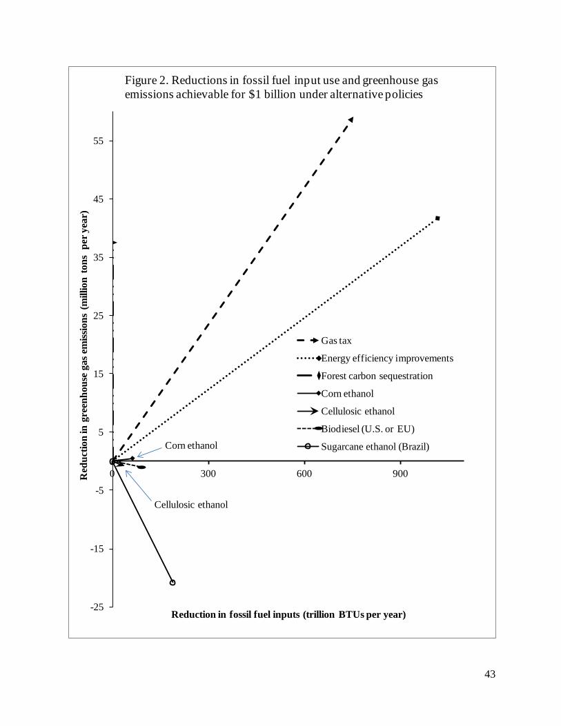
43

Corn ethanol

Cellulosic ethanol

-25

-15

-5

5

15

25

35

45

55

0 300 600 900Red

uctio

n in

gre

enho

use

gas e

miss

ions

(m

illio

n to

ns p

er y

ear)

Reduction in fossil fuel inputs (trillion BTUs per year)

Figure 2. Reductions in fossil fuel input use and greenhouse gas emissions achievable for $1 billion under alternative policies

Gas tax

Energy efficiency improvements

Forest carbon sequestration

Corn ethanol

Cellulosic ethanol

Biodiesel (U.S. or EU)

Sugarcane ethanol (Brazil)

44

U.S. biodiesel

Sugarcane ethanol-50

0

50

100

150

200

250

300

350

400

-1,000 1,000 3,000 5,000 7,000 9,000

Red

uctio

n in

gre

enho

use

gas e

miss

ions

(m

illio

n to

ns p

er y

ear)

Reduction in fossil fuel inputs (trillion BTUs per year)

Figure 3. Potential scale of reduced fossil fuel input use and greenhouse gas emissions with alternative policies

Gas taxEnergy efficiency improvementsForest carbon sequestrationCorn ethanolCellulosic ethanol Soybean biodieselSugarcane ethanol (Brazil)EU Rapeseed Biodiesel

Corn ethanol

45

0

5

10

15

20

25

30

35

40

45

0 1 2 3 4 5 6 7 8 9 10 11 12 13 14 15 16 17 18 19 20

Bill

ions

of

U.S

. dol

lars

Combined reduction in fossil fuel use and GHG emissions: scale indicates percent reduction in gas consumption for gas tax increases

Figure 4. US costs and scope for reducing fossil fuel use and GHG emissions with alternative interventions

Corn ethanol plus forest carbon sequestration (up to 15 B gallons)

Cellulosic switch grass ethanol plus forest carbon sequestration (up to 16 B gallons)

Gas tax

Non-transport energy efficiency improvements

46

0

0.5

1

1.5

2

2.5

3

0 1 2 3 4 5

Bill

ions

of

U.S

. dol

lars

Combined reduction in fossil fuel use and GHG emissions: scale indicates percent reduction in gas consumption for gas tax increases

Figure 5. US costs and scope for reducing fossil fuel use and GHG emissions with alternative interventions

Soybean biodiesel plus forest carbon sequestration (1 B gallons)

Sugarcane ethanol imports from Brazil plus forest carbon sequestration (up to 3 B gallons)Gas tax

Non-transport energy efficiency improvements plus forest carbon sequestration

47

0

5

10

15

20

0 1 2 3 4 5

Bill

ions

of

U.S

. dol

lars

Combined reduction in fossil fuel use and GHG emissions: scale indicates percent reduction in gas consumption for gas tax increases

Figure 6. EU costs and scope for reducing fossil fuel use and GHG emissions with alternative interventions

Gas tax

Oilseed biodiesel (up to 6% of transport fuel) plus forest carbon sequestrationImported sugarcane ethanol from Brazil plus forest carbon sequestration (up to 2 B gallons)

48

Appendix B. Supplemental Materials (online only)

Summary of the economic and technical information used to evaluate each biofuel.

A. Corn ethanol

Estimates of corn ethanol’s economic and technical parameters for production, energy

balance, fossil fuel inputs, and co-product energy credits are taken from a variety of sources

including Iowa State University (Ag Decision Maker 2009), Argonne National Laboratory’s

GREET model (2007), Hill et al. (2006), and Searchinger et al. (2008).

Energy inputs and outputs are from Hill et al. (2006). Ratio of fossil fuel inputs for ethanol

versus gasoline per BTU of energy-in-fuel is 0.57. Ethanol energy in fuel is 76,300 BTU/gal.

Greenhouse gas accounting is from the GREET model (Argonne National Laboratory), cited in

Searchinger et al. (2008). Changes in GHG emissions when substituting corn ethanol for

gasoline include the direct (life cycle) changes in fossil fuel use (a 20,000 gram reduction per

MBTU), plus the indirect land use change effects. For these indirect effects, our base case relies

on estimates by Tyner et al. (2010) for U.S. corn ethanol (a 15,950 g/MBTU increase, for a small

net reduction of 4,100 g/MBTU). The Tyner et al. estimates are based on simulations using

updated base case assumptions and taking account of many of the concerns and criticisms of the

earlier results by Searchinger et al. (2008). For example, they include yield responses to price

increases caused by biofuel production (see also Keeney and Hertel, 2009). Their estimates of

the ILUC effects are about one-seventh as large as Searchinger et al. (2008).7

7 Tyner et al, attribute much of the differences in estimated indirect land use change effects to three factors: 1) their assumptions lead to much smaller land requirements per 1000 gallons of ethanol compared to Searchinger et al.; 2)

49

Prices for corn ethanol, co-product and processing costs are based on average levels from the

past four years based on information from Iowa State University’s Extension Service (Ag

Decision Maker 2009). Implicit subsidies of $0.10/gallon are assumed based on estimated

average direct and counter-cyclical payments to US corn producers (ERS/USDA Briefing

Room/Corn/Policy). The gasoline price is assumed to be $2.00/gallon for cost comparisons based

on EIA data (http://tonto.eia.doe.gov/dnav/pet/hist/d120700002m.htm) for regular gasoline

wholesale (resale) prices 2005-2009. The cost of implementing a substitution of corn ethanol for

gasoline is based on the difference in cost per MBTU plus the cost of subsidies need to equalize

prices to consumers. Our point estimate for the initial marginal cost is $15.70/MBTU of reduced

fossil fuel inputs. Cost per reduction in CO2 emissions are extreme ($2,417/ton CO2-e) due to the

negligible net reductions in GHG emissions arising from the indirect land use change effects.

The supply function for corn ethanol is assumed to reflect rising feedstock costs as corn

ethanol production increases. Based on general equilibrium modeling, Fabioso et al. (2009)

estimate the elasticity of the U.S. corn price with respect to changes in ethanol use to be 0.288;

Elobeid et al. (2007) estimate the same elasticity to be 0.24. With feedstock costs representing

one-third of the cost of ethanol production, the 0.288 elasticity represents an elasticity of ethanol

price of 0.096, or a marginal cost for corn ethanol, MCb, characterized as MCb = MC0 +

0.096∆Q, where ∆Q is the percent increase in US ethanol production above 6.485 gallons. This

implies a 15% increase in cost relative to the base level for U.S. ethanol production of 15 billion

gallons, which is assumed to be the upper bound on U.S. potential production.

their model predicts most land use changes occurring in areas of the world with lower carbon emissions factors; and 3) they assumed only 75% of carbon stored in the forest type vegetations would be released into the atmosphere at the time of land conversion, compared to 100% in the Searchinger et al. model.

50

B. US Soybean biodiesel

As in the case of corn ethanol, many of the economic and technical parameters for soybean

biodiesel production, energy balance, fossil fuel inputs, and co-product energy credits are based

on sources including Iowa State University (Ag Decision Maker 2009), Argonne National

Laboratory’s GREET model (2007), and Hill et al. (2006). Energy inputs and outputs as well as

direct GHG accounting is from Hill et al. (2006). Changes in GHG emissions when substituting

soybean biodiesel for petro diesel include the direct (life cycle) changes in fossil fuel use (a

51,700 gram reduction per MBTU). Indirect land use change effects for biodiesel were not

estimated in Tyner et al. (2009). Searchinger and Heimlich (2007) estimate these to be 198,000

gram/MBTU, however other similar estimates in Searchinger et al. (2007) were about 4 times the

magnitudes estimated by Tyner et al. for corn ethanol. For current purposes we rely on one

additional estimate that is available from CARB (2009b) based on the Purdue University GTAP

model used by Tyner et al. The CARB estimate is 44,300 g/MBTU, which is also about one-

quarter the magnitude of the Searchinger and Heimlich estimate. Given this indirect land use

change effect, the net effect when substituting soybean biodiesel for petroleum diesel is a slight

increase in GHG emissions of 4,300 g/MBTU.

Assumed wholesale or “rack” prices for petroleum diesel are based on a 5 year average from

EIA (http://tonto.eia.doe.gov/dnav/pet/hist/a223700002m.htm). The cost of soybean biodiesel is

estimated to rise with increased production due to rising costs of feedstock production. The

marginal cost MCb is assumed to rise for US production levels according to the relationship

MCb= MC0 (1+0.1875∆Q), where ∆Q is the percent increase in biodiesel production above 2008

levels (0.7 billion gallons). The estimate is based on BRDB 2008 (table 5.1) where reference

cases imply a 0.25 own-price elasticity of supply for soybean production for biodiesel levels

51

above the 700 million gallon level, or a 0.1875 elasticity of biodiesel prices where 75% of the

cost of biodiesel is feedstock cost.

C. US Cellulosic Ethanol from Switchgrass

In the absence of commercial production, estimates of the cost of producing cellulosic

ethanol from perennial grasses such as switchgrass or Miscanthus must be based on field trials,

experiment station trials and engineering estimates (for processing costs). Perrin et al. (2008)

based their estimates on farm-level data over a 5-year period from ten locations in North Dakota,

South Dakota and Nebraska. Those estimates of cost of production are $75/ton of dry matter

when annualized using a 4% discount rate. Duffy (2008) estimates switchgrass costs to be

$90/ton. The cost of collection, storage and transport for switchgrass are estimated by Duffy

(2008) to be $31/ton. Yields of switchgrass per acre averaged 5 ton dry matter in Perrin et al.

(2008). Duffy estimates (based on conditions in Iowa) assumed 4 tons per acre (9 tons/hectare),

whereas the results from Perrin et al. averaged 6.37 tons/ha (excluding initial year yields). A ton

of switchgrass is estimated to produce between 70 and 86 gallons of ethanol. Total costs

including transportation and storage were estimated by Duffy to be $1.51/gallon. Processing

costs are estimated from Wallace et al. (2005) to be $1.52/gallon in 2008 dollars, for a total cost

of $3.03/gallon. The central estimate used here for production, storage and transportation is

$1.51 based on Perrin et al. (2008) and Duffy. When combined with the processing cost estimate

from Wallace et al. of $1.52, the total cost is $3.03/gallon, or $39.71/MBTUs.

Energy inputs and outputs are from Hill et al. 2006. Greenhouse gas accounting is from

the GREET model (Argonne National Laboratory) cited in Searchinger et al. (2008). Indirect

land use change effects are from Searchinger et al. (2008). Future estimates from ongoing

52

research may produce lower values. The direct effects on GHG emissions when substituting

switchgrass-based ethanol for gasoline is a reduction of 90,700 g/MBTU. Indirect effects give

rise to an increase in emissions of 117,100, so that the net effect is an increase of 26,400 g CO2-

e/MBTU.

D. EU biodiesel from rapeseed

Sources for economic and technical information for EU biofuel and energy alternatives

include the International Energy Agency, OECD, and the European Commission. The energy

content of rapeseed-based biodiesel is assumed to be the same as for soybean biodiesel (118,000

BTU/gallon), or about 10 percent lower than petroleum biodiesel. Fossil fuel energy inputs are

about 36% of energy-in-fuel, or 42,000/gallon (JRCEC 2007; IEA 2007). GHG reductions in

emissions when substituting for petroleum diesel are found to be about 54% (, JRCEC 2007; IEA

2004, Searchinger 2007). Few estimates of indirect land use change effects on GHG emissions

for EU rapeseed biodiesel are available. As a result, the estimates described above for soybean

based biodiesel in the US are used.

Biodiesel and other transportation prices for the EU are based on averages over the past 5

years from IEA (2007). Taxes on gasoline in EU are taken from European Commissions data on

energy http://ec.europa.eu/energy/observatory/oil/bulletin_en.htm. Current (2009) figures are

averaging $0.77/liter, or $2.98/gallon tax (this is an average for 2009 for the 27 EU members).

http://ec.europa.eu/energy/reports/Oil_Bulletin_Prices_History.xls. For petro-diesel the tax

averages $0.60/liter. Prices for gasoline excluding taxes are $1.84/gallon). The average gas tax in

the EU is $2.98/gallon. Gasoline consumption in the base case in the EU is about one-third less

than in the U.S. Data on gasoline consumption in the EU: final energy consumption in 2006 is

53

284.7 Mtoe (million tons of oil equivalent) for EU 27 countries. This is from International

Energy Agency 2006 (online

http://www.iea.org/Textbase/stats/balancetable.asp?COUNTRY_CODE=30).

EU gasoline consumption for the baseline is 94.15 billion gallons, or 11,297,809 billion

BTU. Elasticity of demand for gasoline used in the scenarios for gas tax was -0.75. EU biodiesel

production in assumed current base case is 220,506 billion BTU, or 1.5% of total transportation

energy (14,682,7878 billion BTU). The elasticity of oilseed prices with respect to biofuel

production is 0.224, and given an 85% cost share for the feedstock, the elasticity of biofuel cost

with respect to production increases in 0.19. This is based on scenarios from CGE models in

Banse et al., indicating in Table A2 that a policy having a 35.7% increase in oilseed production

will have an 8 percent increase in world oilseed prices. Total transportation fuels in the EU are

14,683,000 billion BTU per year. The EU goal is assumed to be 10% of transportation fuel from

biodiesel, and given an existing 1.5%, that limits the scenarios to additional 8.5 %. This comes at

an equivalent gas tax reducing consumption by 6.9% (gas only – hence this ignores the 20%

share of diesel in transportation fuel).

E. Ethanol from sugarcane, imported from Brazil

The cost of ethanol produced in Brazil has fluctuated in recent years from $0.87/gallon to

more than $1.50/gallon due in part to fluctuations in fossil fuel prices between 2005 and 2008.

An average price over the past four years is in the range of $1.10/gallon FOB. Shipping costs to

the USA would add $0.20 so that, in the absence of the $0.54 import duty, Brazilian ethanol

would have a wholesale price of about $1.30/gallon (Martines-Filho, Burnquist, and Vian 2006).

The energy accounting and life-cycle greenhouse gas accounting for Brazilian ethanol are based

54

on Wang et al. (2007). Fossil fuel inputs are estimated to be only about 3,000 BTU/gallon.

Indirect land use change effects are estimated in Lapola et al. 2010).

Brazil is projected to increase exports were about 1 billion gallons in 2007, and are

expected to increase significantly in coming years (of ethanol to about 1.8 billion gallons by

2015, and to as much as 6.6 billion gallons by 2025. With competing importers from Japan and

the EU, we assume here that the US would only be able to increase imports of Brazilian ethanol

to 3 billion gallons/year.

55

References for Supplemental Materials

Argonne National Laboratory, 2007. “Greenhouse gases, regulated emissions, and energy use in transportation (GREET) computer model.” (www.transportation.anl.gov/software/GREET/publications.html).

Banse, B., Hans van Meijl , Andrzej Tabeau , and Geert Woltjer, 2008. Will EU biofuel policies affect global agricultural markets? European Review of Agricultural Economics. DOI 10.1093/erae/jbn023. Eur Rev Agric Econ 35: 117-141.

BRDB (U.S. Biomass Research and Development Board), 2008. Increasing feedstock production for biofuels: economic drivers, environmental implications, and the role of research. (www.usbiomassboard.gov/pdfs/8_Increasing_Biofuels_Feedstock_Production.pdf)

EIA (U.S. Energy Information Agency), 2009. Petroleum Marketing Monthly, Explanatory Notes (http://www.eia.doe.gov/pub/oil_gas/petroleum/data_publications/petroleum_marketing_monthly/current/pdf/enote.pdf, accessed December 2009).

CARB (California Air Resources Board, 2009a. Staff Report: Initial Statement of Reasons Proposed Regulation to Implement the Low Carbon Fuel Standard: volume 1. http://www.arb.ca.gov/fuels/lcfs/030409lcfs_isor_vol1.pdf (accessed 8/18/2009).

CARB (California Air Resources Board, 2009b. Detailed California-Modified GREET Pathway for Biodiesel (Esterified Soyoil) from Midwest Soybeans. http://www.arb.ca.gov/fuels/lcfs/022709lcfs_biodiesel.pdf (accessed 8/24/2009).

Duffy, M. 2008. Estimating costs of production, storage and transportation of switchgrass. Ag Decision Maker File A1-22, February (www.extension.iastate.edu/agdm).

Elobeid, A., Tokgoz, S., Hayes, D.J., Babcock, B.A., & Hart, C.E. (2007). The long-run impact of corn-based ethanol on the grain, oilseed, and livestock sectors with implications for biotech crops. AgBioForum, 10(1), 11-18 (http://www.agbioforum.org).

International Energy Agency (IEA), 2004. Biofuels for Transport: An International Perspective. IEA, Paris.

International Energy Agency (IEA), 2007. IEA Energy Technology Essentials: Biofuel Production (ETE02). (http://www.iea.org/Textbase/techno/essentials2.pdf).

Iowa State University Extension, "Ag Decision Maker", accessed 2/2/2009. (www.extension.iastate.edu/agdm/).

JRCEC (Joint Research Center of the European Commission), 2007. Well-to-wheels analysis of future automotive fuels and powertrains in the European context. Version 2c. March. http://ies.jrc.ec.europa.eu/WTW.

56

Keeney, R. and T.W. Hertel, 2009. The indirect land use impacts of United States biofuel policies: the importance of acreage, yield, and bilateral trade responses. Amer. J. Agr. Econ. 91(4): 895-909.

Lapola, D.M, R. Schaldach, J. Alcamo, A. Bondeau, J Koch, C. Koelking, and J.A. Priess, 2010. Indirect land-use changes can overcome carbon savings from biofuels in Brazil. Proceedings of the national Academy of Sciences, Vo. 107(8), 3388-3393.

Perrin, R., Vogel, K.P., Schmer, M.R., Mitchell, R. 2008. Farm-scale Production Cost of Switchgrass for Biomass. BioEnergy Research 1:91-97 (http://www.springerlink.com/content/f85977006m871205/).

Searchinger, T.D. and R. Heimlich, 2007. Estimating greenhouse gas emissions from soy-based U.S. biodiesel when factoring in emissions from land use change. Paper prepared for workshop on the lifecycle carbon footprint of biofuels organized by the Farm Foundation and the U.S. Department of Agriculture, Jan. 29, 2008 (http://www.farmfoundation.org/news/articlefiles/371-Searchinger%203-12-08.pdf)

Tyner, W.E., F. Taheripour, Q. Zhuang, D. Birur and U. Baldos, 2010. Land use change and consequent CO2 emissions due to US corn ethanol production: a comprehensive analysis: Final Report. April 2010. Department of Agricultural Economics, Purdue University.

Wallace, R., Ibsen, K., McAloon, A..W. Yee, 2005. Feasibility study for co–locating and integrating ethanol production plants from corn starch and lignocellulogic feedstocks, NREL/TP–510–37092. USDA/USDOE/NREL, Revised Edition. Golden, Colorado.

Wang, M., M. Wu, J. Huo, and J. Liu, 2007. Well-to-Wheels Energy Use and Greenhouse Gas Emissions of Brazilian Sugarcane Ethanol Production Simulated by Using the GREET Model. Center for Transportation Research, Argonne National Laboratory. July 20.