Seediscussions,stats,andauthorprofilesforthispublicationat:https://www.researchgate.net/publication/228805202

TheCostsofAdaptationtoClimateChangeinCanada:Astratifiedestimatebysectorsandregions

Article·May2001

CITATIONS

18

READS

180

4authors,including:

Someoftheauthorsofthispublicationarealsoworkingontheserelatedprojects:

ResiliencetonaturaldisastersinBangladeshViewproject

Thegenericandrootcausesofdisasters.Viewproject

MohammedDore

BrockUniversity

99PUBLICATIONS778CITATIONS

SEEPROFILE

IanBurton

UniversityofToronto

150PUBLICATIONS8,414CITATIONS

SEEPROFILE

AllcontentfollowingthispagewasuploadedbyMohammedDoreon21May2014.

Theuserhasrequestedenhancementofthedownloadedfile.

The Costs of Adaptation to Climate Change in Canada: A Stratified

Estimate by Sectors and Regions

Social Infrastructure

By

Mohammed H.I. Dore

Brock University

and

Ian Burton

A.I.R.G., Environment Canada

April 17, 2001 Mohammed Dore, D.Phil. (Oxon) Climate Change Laboratory Taro Hall, Room 442 Brock University St Catharines, ON Canada L2S 3A1 Tel. (905) 688 5550, ext 4755 Email: dore@adam.econ.brocku.ca This research was financed by a grant from the Canadian Climate Change Action Fund under grant No. A209. However, the opinions expressed are those of the authors alone.

1

The Costs of Adaptation to Climate Change in Canada: A Stratified Estimate by Sectors and Regions

Social Infrastructure

Table of Contents

Preface............................................................................................................................... 11 Executive Summary .......................................................................................................... 12

Progress to Date on the Estimation of Adaptation Costs............................................... 12 Detailed Executive Summary ........................................................................................ 12

Chapter 1: Data Collection Protocol ................................................................................. 20 1.1: Introduction ............................................................................................................ 20 Figure 1.1.1: Ecoclimatic Provinces of Canada and Projected Shifts Under a Scenario of Doubled Atmospheric Carbon Dioxide..................................................................... 24 1.2: Anticipated Effects of Climate Change.................................................................. 28 1.3: Methodology .......................................................................................................... 29

1.3.1: Definitions of Sectors of the Economy ............................................................ 29 1.3.2: Sampling Structure........................................................................................... 32 1.3.3: Spatial Methods................................................................................................ 32 1.3.4: Quantitative Estimation Methods..................................................................... 33 1.3.5: Base Maps ........................................................................................................ 34

Figure 1.3.1: CGCM1 Grid Boxes Overlaid on Census Subdivisions .......................... 35 1.3.6: Codes and Standards ........................................................................................ 36 1.3.7: Climate Change Factors ................................................................................... 37 1.3.8: Statistics Canada Census 1996......................................................................... 40 1.3.9: Municipal Financial Information ..................................................................... 40 1.3.10: Historical Climate Information ...................................................................... 42

1.4: Directions for Future Research............................................................................... 42 1.4.1: Climate Data..................................................................................................... 43 1.4.2: Census Subdivision Data ................................................................................. 43 1.4.3: Government Financial Data ............................................................................. 43

1.4.3.1: Municipal Financial Information ............................................................... 44 1.4.3.2: Provincial Financial Information ............................................................... 44 1.4.3.3: Federal Financial Information ................................................................... 45 1.4.3.4: Other Government Agencies ..................................................................... 45

1.4.4: Other Data Sources .......................................................................................... 45 1.5: Summary ................................................................................................................ 46

Chapter 2: Climate Change Projections............................................................................ 48 2.1: Downscaling Experiment with SDSM ................................................................... 48

2

Table 2.1.1: from SDSM: Daily Precipitation Data for Toronto, 1981-1990 ............... 49 Table 2.1.2: Testing the Toronto Data........................................................................... 51 Table 2.1.3: SDSM Summary Statistics using GCM Independent Variables ............... 52 Table 2.1.4: Summary Statistics for the Projected Precipitation for Toronto, 2050s.... 53 2.2: Proportional Downscaling...................................................................................... 55 2.3: Understanding Climate Change.............................................................................. 57 Figure 2.3.1: Fitted Values With 95% Confidence Intervals for ARIMA (1,0,0) Model....................................................................................................................................... 59 2.4: Summary and Directions For Future Research ...................................................... 60 References: .................................................................................................................... 62

Chapter 3: The Theory Of The Optimal Production Of Public Goods And Its Application To Social Infrastructure .................................................................................................... 63

3.1 The Optimal Quantity of a Public Good.................................................................. 65 3.2 The Changing Nature of a Public Good .................................................................. 67 3.3 Climate Change and Social Infrastructure............................................................... 71 3.4 Summary and Directions for Future Research ........................................................ 73 References: .................................................................................................................... 75

Chapter 4: Roads and Bridges in Canada ......................................................................... 76 4.1: Introduction ............................................................................................................ 76 4.2: Basic Climate Information ..................................................................................... 79 4.3: Roads, Bridges and Storm Water Management Jurisdiction in Canada................. 79 Table 4.3.1: Road Jurisdiction in Canada (2-lane equivalent) ...................................... 81 Table 4.3.2: Bridge Jurisdiction in Canada* ................................................................. 82 4.4: Roads, Bridges and Storm Water Management System Design Codes and Standards ....................................................................................................................... 83

4.4.1: Roads................................................................................................................ 85 Table 4.4.3: Road Type Distribution in Canada (1995) ................................................ 86

4.4.1.1: Alberta ....................................................................................................... 86 Table 4.4.4: Road Type Distribution in Alberta (1995) ................................................ 87

4.4.1.2: British Columbia........................................................................................ 87 Table 4.4.5: Road Type Distribution in British Columbia (1995)................................. 87

4.3.1.3 Manitoba ..................................................................................................... 88 Table 4.4.6: Road Type Distribution in Manitoba (1995)............................................. 88

4.4.1.4: New Brunswick.......................................................................................... 88 Table 4.4.7: Road Type Distribution in New Brunswick (1995) .................................. 89

4.4.1.5: Newfoundland............................................................................................ 89 Table 4.4.8: Road Type Distribution in Newfoundland (1995) .................................... 89

4.4.1.6: Nova Scotia................................................................................................ 89 Table 4.4.9: Road Type Distribution in Nova Scotia (1995)......................................... 90

4.4.1.7: Ontario ....................................................................................................... 90 Table 4.4.10: Road Type Distribution in Ontario (1995) .............................................. 91

4.4.1.8: Prince Edward Island ................................................................................. 91 Table 4.4.11: Road Type Distribution in Prince Edward Island (1995)........................ 91

4.4.1.9: Quebec ....................................................................................................... 91 Table 4.4.12: Road Type Distribution in Quebec (1995) .............................................. 92

4.4.1.10: Saskatchewan........................................................................................... 92

3

Table 4.4.13: Road Type Distribution in Saskatchewan (1995).................................... 92 4.4.1.11: Northwest Territories............................................................................... 93

Table 4.4.14: Road Type Distribution in Northwest Territories (1995)........................ 93 4.4.1.12: Nunavut.................................................................................................... 94

Table 4.4.15: Road Type Distribution in Nunavut (1995) ............................................ 94 4.4.1.13: Yukon....................................................................................................... 94

Table 4.4.16: Road Type Distribution in Yukon (1995) ............................................... 95 4.4.2: Bridges ............................................................................................................. 95

4.4.2.1: Alberta ....................................................................................................... 95 4.4.2.2: British Columbia........................................................................................ 96 4.4.2.3: Manitoba .................................................................................................... 96 4.4.2.4: New Brunswick.......................................................................................... 96 4.4.2.5: Newfoundland............................................................................................ 96 4.4.2.6: Nova Scotia................................................................................................ 97 4.4.2.7: Ontario ....................................................................................................... 97 4.4.2.8: Prince Edward Island ................................................................................. 97 4.4.2.9: Quebec ....................................................................................................... 98 4.4.2.10: Saskatchewan........................................................................................... 98 4.4.2.11: Northwest Territories............................................................................... 98 4.4.2.12: Nunavut.................................................................................................... 98 4.4.2.13: Yukon....................................................................................................... 99

4.4.3: Storm Water Management ............................................................................... 99 4.4.3.1: Alberta ....................................................................................................... 99 4.4.3.2: British Columbia........................................................................................ 99 4.4.3.3: Manitoba .................................................................................................. 100 4.4.3.4: New Brunswick........................................................................................ 100 4.4.3.5: Newfoundland.......................................................................................... 100 4.4.3.6: Nova Scotia.............................................................................................. 100 4.4.3.7: Ontario ..................................................................................................... 101 4.4.3.8: Prince Edward Island ............................................................................... 101 4.4.3.9: Quebec ..................................................................................................... 102 4.4.3.10: Saskatchewan......................................................................................... 102 4.4.3.11: Northwest Territories............................................................................. 102 4.4.3.12: Nunavut.................................................................................................. 103 4.4.3.13: Yukon..................................................................................................... 103

4.5: The Major Components of Costs and Associated Climate Factors...................... 103 4.5.1: Capital Costs .................................................................................................. 105

4.5.1.1: Roads ....................................................................................................... 106 Table 4.5.1: Highway Expenditures in Canada (paved, surface treated and gravel) Level by Province/Territory for all Jurisdictions................................................................... 111

4.5.1.2: Bridges ..................................................................................................... 112 Table 4.5.2: Bridge Type and Temperature Design Standards (OHBDC).................. 118 Table 4.5.3: Differences in Wind Effects on Bridge Components.............................. 119 Table 4.5.4 Ice Loads Imposed by Moving Ice ........................................................... 120

4.5.1.3: Ditches and Drains................................................................................... 121 4.5.2: Operating Costs.............................................................................................. 125

4

4.5.2.1: Roads ....................................................................................................... 125 4.5.2.2: Bridges ..................................................................................................... 127 4.5.2.3: Ditches and Drains................................................................................... 131 4.5.2.4: Winter Control ......................................................................................... 131

4.5.3: Summary ........................................................................................................ 133 4.5.3.1: Roads Capital Costs ................................................................................. 133 4.5.3.2: Roads Operating Costs ............................................................................ 134 4.5.3.3: Bridges Capital Costs............................................................................... 134 4.5.3.4: Bridges Operating Costs .......................................................................... 135 4.5.3.5: Storm Water Management System Capital Costs.................................... 136 4.5.3.6: Storm Water Management Operating Costs ............................................ 136

4.6: The Costs of Adaptation....................................................................................... 137 4.6.1: Capital Costs .................................................................................................. 137

4.6.1.1: Roads ....................................................................................................... 137 4.6.1.1.1: All Roads ........................................................................................... 138 4.6.1.1.2: Winter/Ice Roads ............................................................................... 139

Table 4.6.1: Summary of Quantity and Distribution of Winter/Ice Roads in Canada 140 Table 4.6.2: Opening and Maintenance Costs for Winter/Ice Roads .......................... 141 Table 4.6.3: Mean Winter Temperatures 1961-1990, 2010-2039, 2040-2069, 2070-2099 ............................................................................................................................. 144 Table 4.6.4: Grid Boxes With Potentially Complete Loss of Winter/Ice Roads (mean winter temperatures higher than –20 C)....................................................................... 147 Table 4.6.5: Grid Boxes With Shortening of Winter/Ice Road Season (mean winter temperatures between –20 C and –40 C) ...................................................................... 148 Table 4.6.6: Grid Boxes With Little/No Impact on Winter/Ice Roads (mean winter temperatures remain below –40 C) .............................................................................. 148 Table 4.6.7: Provincial Temperature Scenarios for Grid Boxes within Winter/Ice Road Zone by 2100............................................................................................................... 149 Table 4.6.8: Provincial Replacement Scenarios for Grid Boxes within Winter/Ice Road Zone by 2100............................................................................................................... 150 Figure 4.6.1: Winter/Ice Road Replacement (km) by the Year 2100.......................... 151 Table 4.6.9: Climate Change Adaptation Costs for Winter/Ice Road Replacement by Province (Year 2100)................................................................................................... 152

4.6.1.1.3: Roads on Permafrost.......................................................................... 152 Table 4.6.10: Temperature Changes in the Grid Boxes Within the Discontinuous Permafrost Zone (all values in °C) .............................................................................. 156 Figure 4.6.2: Temperature Distribution (°C) for Grid Boxes Within Discontinuous Permafrost Zone .......................................................................................................... 158 Table 4.6.11 Temperature Changes Within Grid Boxes Located Within Discontinuous Permafrost Zone .......................................................................................................... 158

4.6.1.2: Bridges ..................................................................................................... 159 4.6.1.2.1: Inland Bridges ................................................................................... 161 4.6.1.2.2: Coastal Bridges.................................................................................. 161

Table 4.6.12: Number of Coastal Bridges in Canada .................................................. 163 Table 4.6.13: Coastal Bridge Replacement by Province ............................................. 165 Figure 4.6.3: Coastal Bridge Replacement by Province by the Year 2100 ................. 166

5

Figure 4.6.4: Proportion of Coastal Bridge Replacement Costs by Province ............. 166 Table 4.6.14: Coastal Bridge Replacement by Province (Year 2100)......................... 167

4.6.1.2.3: Bridges Over Water........................................................................... 167 4.6.1.3: Ditches and drains.................................................................................... 168

4.6.2: Operating Costs.............................................................................................. 168 4.6.2.1: Roads ....................................................................................................... 169

Table 4.6.14: Approximate Number of Freeze-Thaw Cycles in Heavily Populated Areas of Canada........................................................................................................... 169

4.6.2.2: Bridges ..................................................................................................... 171 4.6.2.2.1: Salt Application on Bridges............................................................... 172

4.6.2.3: Ditches and Drains................................................................................... 174 4.6.2.4: Winter Control ........................................................................................ 174

Figure 4.6.5: Winter Control Expenditure Versus Annual Snowfall (per km of road)178 Table 4.6.15 Winter Control Costs – Selected Municipalities .................................... 178 Table 4.6.16: Projected Cost Changes for Winter Control to 2030............................. 181

4.6.3: Directions for Future Research ...................................................................... 182 4.6.3.1: Roads ....................................................................................................... 182 4.6.3.2: Bridges ..................................................................................................... 183 4.6.3.3: Storm Water Management Systems......................................................... 184

4.6.4: Summary ........................................................................................................ 185 References: .................................................................................................................. 189 Appendix 4.6.1: ........................................................................................................... 192 Standards for Ice Road Use – White Ice...................................................................... 192 Standards for Ice Road Use – Blue Ice........................................................................ 193 Appendix 4.6.2: ........................................................................................................... 195 Winter Temperatures 1961-1990 (Baseline) ............................................................... 195 Winter Temperatures 2010-2039................................................................................. 196 Winter Temperatures 2040-2069................................................................................. 198 Winter Temperatures 2070-2099................................................................................. 199 Appendix 4.6.3: ........................................................................................................... 201 Projected Changes in Snowfall for all Grid Boxes to 2100......................................... 201

Chapter 5: Drinking Water Supply and Wastewater Treatment ..................................... 212 5.1: Water in Canada: An Introduction ....................................................................... 212

5.1.1: The Cost of Water in Canada ......................................................................... 215 5.1.2: Water Prices in Canada .................................................................................. 216 5.1.3: The Implications of Climate Change for Municipal Water Infrastructure..... 217 5.1.4: Potential Adaptations of Municipal Water Infrastructure.............................. 220

5.2: Toronto, ON ......................................................................................................... 221 5.2.1: Introduction .................................................................................................... 221

Figure 5.2.1: Toronto and Niagara .............................................................................. 222 5.2.2: Great Lake Levels .......................................................................................... 222 5.2.3: The Water Supply Services Component ........................................................ 224 5.2.4: Water Supply and Adaptation to Climate Change ......................................... 225 5.2.5: The Wastewater Services Component ........................................................... 225 5.2.6: The Major Components of Cost..................................................................... 226

5.2.6.1: Capital Costs ............................................................................................ 226

6

Table 5.2.1: Capital Assets –Water and Wastewater Services Division ..................... 226 5.2.6.2: Operating Costs........................................................................................ 226

Table 5.2.2: 1999 Water Services Budget Less Debt Charges.................................... 227 Table 5.2.3: 1999 Wastewater Services Budget Less Debt Charges........................... 227

5.2.7: Water Production Statistics ............................................................................ 227 Table 5.2.4: Potable Water Production........................................................................ 228 Table 5.2.5: 1999 Water Consumption by Toronto Communities .............................. 228 Table 5.2.6: Plant Capacities & Average Daily Flows................................................ 228 Table 5.2.7: Pumping Station Capacities..................................................................... 229 Table 5.2.8: Precipitation Descriptive Statistics for Toronto ...................................... 229

5.2.8: Regression Analysis ....................................................................................... 229 5.2.9: Graphical Results ........................................................................................... 231

Figure 5.2.2: Results for Toronto (1961-1990) ........................................................... 231 Figure 5.2.3: Results for Toronto (2010-2039) ........................................................... 231 Figure 5.2.4: Results for Toronto (2040-2069) ........................................................... 232 Figure 5.2.5: Results for Toronto (2070-2099) ........................................................... 233

5.2.10: Methodology ................................................................................................ 233 Table 5.2.9: Predicted Precipitation to Exceed Toronto’s Present Wastewater Capacity..................................................................................................................................... 234 Table 5.2.10: Upper Confidence Interval to Exceed Toronto’s Present Wastewater Capacity ....................................................................................................................... 235

5.2.11: Optimal Adaptation Costs of Wastewater Infrastructure for Toronto ......... 235 Figure 5.2.6: Waste Water Process.............................................................................. 236

5.2.11.1: Experiment 1.......................................................................................... 237 Figure 5.2.7: Solution – Experiment 1 ........................................................................ 238

5.2.11.2: Experiment 2.......................................................................................... 238 Figure 5.2.8: Solution – Experiment 2 ........................................................................ 239

5.2.11.3: Experiment 3.......................................................................................... 239 Figure 5.2.9: Solution – Experiment 3 ........................................................................ 240

5.2.11.4: Experiment 4.......................................................................................... 240 Figure 5.2.10: Solution – Experiment 4 ...................................................................... 241

5.2.11.5: Experiment 5 Extreme Event................................................................. 241 Figure 5.2.11: Solution – Experiment 5 ...................................................................... 242

5.2.12: Combined Sewers......................................................................................... 242 5.2.13: Total Cost of Adaptation.............................................................................. 243 5.2.14: Summary and Conclusion ............................................................................ 244

5.3: Niagara, ON.......................................................................................................... 244 5.3.1: Precipitation Trends ....................................................................................... 246 5.3.2: Precipitation and Water Flow......................................................................... 247 5.3.3: Niagara River Drainage, Lake Erie and Lake Ontario................................... 247

Table 5.3.1: Average Flow Water Rates...................................................................... 248 5.3.4: Drinking Water Supply Impacts..................................................................... 248

5.3.4.1: Capital Costs ............................................................................................ 248 5.3.4.2: Operating Costs........................................................................................ 248 5.3.4.3: Capital Projects ........................................................................................ 249

5.3.5: Wastewater Treatment ................................................................................... 249

7

5.3.5.1: Climate Induced Change in the Rainfall.................................................. 249 5.3.5.2: General Circulation Model-CGCM1 Greenhouse Gas Only Simulation 250 5.3.5.3: CGCM1-GG1 Proportional Downscaling ............................................... 251

Table 5.3.2: CGCM1-GG1 Proportional Downscaled Precipitation Statistics for Niagara......................................................................................................................... 251

5.3.5.4: Regression Results................................................................................... 251 Figure 5.3.1: Results for Niagara (1961-1990)............................................................ 253 Figure 5.3.2: Results for Niagara (2010-2039)............................................................ 253 Figure 5.3.3: Results for Niagara (2040-2069)............................................................ 254 Figure 5.3.4: Results for Niagara (2070-2099)............................................................ 254

5.3.5.5: Capacities and Flows ............................................................................... 255 Table 5.3.3: Wastewater Treatment Plant and Lagoon Flow Ratings ......................... 255 Table 5.3.4: Predicted Precipitation to Exceed Niagara’s Wastewater Capacity........ 256 Table 5.3.5: Upper Confidence Level to Exceed Niagara’s Wastewater Capacity..... 256

5.3.5.6: Capital Costs ............................................................................................ 257 5.3.6: Costs of Adaptation........................................................................................ 257 5.3.7: Summary and Conclusion .............................................................................. 258

5.4: Montreal, PQ ........................................................................................................ 258 5.4.1: Drinking Water Supply .................................................................................. 258

Figure 5.4.1: Communité Urbaine de Montréal .......................................................... 259 5.4.2: CGCM1-GG1 Proportional Downscaling...................................................... 259

Table 5.4.1: CGCM1-GG1 Proportional Downscaled Descriptive Precipitation Statistics....................................................................................................................... 260

5.4.3: Wastewater Treatment ................................................................................... 260 Table 5.4.2 Average Flows and Treated Volumes ...................................................... 263

5.4.4: Wastewater Treatment Plant Costs ................................................................ 264 5.4.5: Regression Results ......................................................................................... 264

Figure 5.4.2: Results for Montreal (1961-1990).......................................................... 265 Figure 5.4.3: Results for Montreal (2010-2039).......................................................... 266 Figure 5.4.4: Results for Montreal (2040-2069).......................................................... 266 Figure 5.4.5: Results for Montreal (2070-2099).......................................................... 267

5.4.6: Summary and Conclusion .............................................................................. 267 5.5: Halifax, NS........................................................................................................... 267

5.5.1: Drinking Water Supply .................................................................................. 268 Figure 5.5.1: Halifax.................................................................................................... 268

5.5.2: Wastewater Treatment ................................................................................... 268 Table 5.5.1 Descriptive Precipitation Statistics for Halifax ........................................ 269

5.5.3: Regression Results for Halifax....................................................................... 269 Figure 5.5.2: Results for Halifax (1961-1990) ............................................................ 271 Figure 5.5.3: Results for Halifax (2010-2039) ............................................................ 271 Figure 5.5.4: Results for Halifax (2040-2069) ............................................................ 272 Figure 5.5.5: Results for Halifax (2070-2099) ............................................................ 272 Table 5.5.2: Upper Confidence Level to Exceed Halifax’s Wastewater Capacity...... 273

5.5.4: Costs of Adaptation........................................................................................ 273 5.5.5: Summary and Conclusion .............................................................................. 274

5.6: The Prairies........................................................................................................... 274

8

5.6.1: Regina, SK ..................................................................................................... 275 Figure 5.6.1: Regina .................................................................................................... 276 5.6.1.2: Buffalo Pound Lake........................................................................................ 276 Table 5.6.1: 1999 Water Sales (mega litres) ............................................................... 277 Table 5.6.2: Annual Raw Water Production................................................................ 278

5.6.1.3: Operations and Capital Projects............................................................... 278 5.6.2: Drinking Water Supply .................................................................................. 279

Table 5.6.3: Monthly Drinking Water Production, 2000 ............................................ 281 5.6.3: Wastewater Treatment ................................................................................... 282

Table 5.6.4: Precipitation Descriptive Statistics for Regina........................................ 282 5.6.4: Regression Results ......................................................................................... 283

Figure 5.6.2: Results for Regina (1961—1990) .......................................................... 284 Figure 5.6.3: Results for Regina (2010-2039)............................................................. 284 Figure 5.6.4: Results for Regina (2040-2069)............................................................. 285 Figure 5.6.5: Results for Regina (2070-2099)............................................................. 285

5.6.5: Summary and Conclusion .............................................................................. 285 5.7: Humboldt, SK....................................................................................................... 286 Figure 5.7.1: Humboldt ............................................................................................... 287

5.7.1: Drinking Water Supply and Sask Water ........................................................ 287 Table 5.7.1: Humboldt Precipitation Descriptive Statistics ........................................ 288

5.7.2: Regression Results ......................................................................................... 288 Figure 5.7.2: Results for Humboldt (1961-1990) ........................................................ 290 Figure 5.7.3: Results for Humboldt (2010-2039) ........................................................ 290 Figure 5.7.4: Results for Humboldt (2040-2069) ........................................................ 291 Figure 5.7.5: Results for Humboldt (2070-2099) ........................................................ 291

5.7.3: Summary and Conclusions............................................................................. 292 5.8: Swift Current, SK ................................................................................................. 292

5.8.1: Drinking Water Supply .................................................................................. 292 Figure 5.8.1: Swift Current.......................................................................................... 293 Table 5.8.1: Precipitation Descriptive Statistics for Swift Current ............................. 293

5.8.2: Regression Results ......................................................................................... 293 Figure 5.8.2: Results for Swift Current (1961-1990) .................................................. 295 Figure 5.8.3: Results for Swift Current (2010-2039) .................................................. 295 Figure 5.8.4: Results for Swift Current (2040-2069) .................................................. 296 Figure 5.8.5: Results for Swift Current (2070-2099) .................................................. 296

5.8.3: Summary and Conclusions............................................................................. 297 5.9: Lethbridge, AB..................................................................................................... 297

5.9.1: Drinking Water Supply .................................................................................. 297 Figure 5.9.1: Lethbridge .............................................................................................. 297 Table 5.9.1: Ten Year Average Water Production in Millions of Litres (ML) ........... 298

5.9.2: Wastewater Treatment ................................................................................... 299 Table 5.9.2: Descriptive Precipitation Statistics for Lethbridge ................................. 300

5.9.3: Regression Results ......................................................................................... 300 Figure 5.9.2: Results for Lethbridge (1961-1990)....................................................... 301 Figure 5.9.3: Results for Lethbridge (2010-2039)....................................................... 302 Figure 5.9.4: Results for Lethbridge (2040-2069)....................................................... 302

9

Figure 5.9.5: Results for Lethbridge (2070-2099)....................................................... 303 Table 5.9.3: Upper Confidence Level Exceeding Lethbridge’s Present Wastewater Capacity ....................................................................................................................... 303

5.9.4: Costs of Adaptation........................................................................................ 304 5.9.5: Summary and Conclusions............................................................................. 304

5.10: Prince George, BC.............................................................................................. 304 5.10.1: Drinking Water Supply ................................................................................ 304

Figure 5.10.1: Prince George....................................................................................... 305 Table 5.10.1: Monthly Water Production 2000........................................................... 306

5.10.2: Wastewater Treatment ................................................................................. 306 Table 5.10.2: Monthly Wastewater Flows 2000.......................................................... 307 Table 5.10.3: Prince George Descriptive Statistics ..................................................... 307

5.10.3: Regression Results ....................................................................................... 307 Figure 5.10.2: Results for Prince George (1961-1990) ............................................... 309 Figure 5.10.3: Results for Prince George (2010-2039) ............................................... 309 Figure 5.10.4: Results for Prince George (2040-2069) ............................................... 310 Figure 5.10.5: Results for Prince George (2070-2099) ............................................... 310

5.10.4: Summary and Conclusions........................................................................... 311 5.11: Penticton, BC...................................................................................................... 311

5.11.1: Drinking Water Supply ................................................................................ 311 Figure 5.11.1: Pentiction ............................................................................................. 312 Table 5.11.1: Daily Consumption of Water ................................................................ 312

5.11.2: Wastewater Treatment ................................................................................. 313 Table 5.11.2: Average Daily Flow (ML/Day)............................................................. 313 Table 5.11.3: Penticton Precipitation Descriptive Statistics........................................ 313

5.11.3: Regression Results ....................................................................................... 314 Figure 5.11.2: Results for Penticton (1961-1990) ....................................................... 315 Figure 5.11.3: Results for Penticton (2010-2039) ....................................................... 315 Figure 5.11.4: Results for Pentiction (2040-2069) ...................................................... 316 Figure 5.11.5: Results for Penticton (2070-2099) ....................................................... 316 Table 5.11.4: Precipitation Exceeding Penticton’s Present Wastewater Capacity...... 317 Table 5.11.5: Upper Confidence Interval Exceeding Penticton’s Present Wastewater Capacity ....................................................................................................................... 317

5.11.4: Costs of Adaptation...................................................................................... 318 5.11.5: Summary and Conclusions........................................................................... 318

5.12: Yellowknife, NT................................................................................................. 318 5.12.1: Drinking Water Supply ................................................................................ 318

Figure 5.12.1: Yellowknife.......................................................................................... 319 5.12.2: Permafrost and Climate Change................................................................... 319 5.12.3: Wastewater Treatment ................................................................................. 319

Table 5.12.1: Yellowknife Descriptive Statistics ........................................................ 320 5.12.4: Regression Results ....................................................................................... 320

Figure 5.12.2: Results for Yellowknife (1961-1990) .................................................. 321 Figure 5.12.3: Results for Yellowknife (2010-2039) .................................................. 322 Figure 5.12.4: Results for Yellowknife (2040-2069) .................................................. 322 Figure 5.12.5: Results for Yellowknife (2070-2099) .................................................. 323

10

5.12.5: Summary and Conclusion ............................................................................ 323 5.13: Norman Wells, NT ............................................................................................. 323

5.13.1: Drinking Water Supply ................................................................................ 323 Figure 5.13.1: Norman Wells ...................................................................................... 324

5.13.2: Wastewater Treatment ................................................................................. 325 Table 5.13.1: Water Consumption and Wastewater Flows, 2000 (m3) ....................... 325

5.13.3: Permafrost and Climate Change................................................................... 325 Table 5.13.2: Norman Wells Descriptive Statistics..................................................... 326

5.13.4: Regression Results ....................................................................................... 326 Figure 5.13.2: Results for Norman Wells (1961-1990)............................................... 327 Figure 5.13.3: Results for Norman Wells (2010-2039)............................................... 328 Figure 5.13.4: Results for Norman Wells (2040-2069)............................................... 328 Figure 5.13.5: Results for Norman Wells (2070-2099)............................................... 329

5.13.5: Summary and Conclusions........................................................................... 329 5.14: Directions for Future Research........................................................................... 329 5.15: Summary............................................................................................................. 332 References: .................................................................................................................. 337

11

Preface This research was carried out under the CCAF Grant No. A209. Under the same grant, we earlier wrote a review of the literature. It was entitled: The Costs of Adaptation to Climate Change: a Critical Review, dated November 15, 2000. The present work should be seen as a continuation of that work. As with the earlier report, this work should be of interest to three kinds of readers: the specialized climate change scientists and researchers in the field of adaptations and impacts of climate change; readers interested in policy formation, and the top level decision makers. We expect that the scientists and researchers will want to read the entire report. Those interested in policy formation may read the comprehensive summary of each chapter, and the top-level decision makers with very little time may want to read the Executive Summary. We are again fortunate in receiving assistance from a larger number of people. First we would like to thank all those who responded to our questionnaires, which were followed by emails and phone calls to all managers, engineers, and civil servants who look after Canada’s roads and water utilities. We consulted people at the federal, provincial, regional and municipal levels all over Canada. Without their generous support of time and their willingness to share their data this study would not have been possible. At Brock University, we would like to thank Kathleen Jaques Bennett, Indra Hardeen, Mike Patterson, Harvey Stevens, and Klemen Zumer who all worked at one time or the other at the Climate Change Laboratory at Brock University. We would also like to thank Dr.Elaine Barrow, Dr.Eva Mekis, Trevor Murdock, Dr.Elaine Wheaton and Dr.Francis Zwiers. In addition we continued to receive generous help from two librarians at Brock University: Margaret Dore and Moira Russell. As usual, Margaret also did a fair amount of unpaid proof reading and editing. At Environment Canada we would like to thank Indra Fung-Fook, Ash Kumar and Roberta McCarthy. However, the remaining deficiencies are those of the two authors alone.

12

Executive Summary

Progress to Date on the Estimation of Adaptation Costs We have made a beginning on the estimation of adaptation costs of climate change for social infrastructure. On roads, we estimate that the cost of constructing an all weather road is $85 000 per km plus an additional $65 000 to $150 000 per bridge. The cost on permafrost is $500 000 per km and $350 000 per km on non-permafrost land. An average coastal bridge will cost $600 000, with a total expected cost of all coastal bridges being around $9 billion. The most important operating cost for roads is winter control, which we estimate to be between $9 and $12 per km. For water utilities the adaptation costs will be mainly in the form of expanding wastewater treatment capacity. For Toronto, the adaptation costs range from $633 million to $9 billion; for Niagara between $8 and $24 million; for Halifax about $6.5 million. Montreal is an exception as it has excess capacity. These estimates are based on case studies and cannot be extrapolated regionally or nationally because Canada has a number of distinct ecoclimatic zones. We report on other case studies too, covering the entire country, but these case studies need to be extended to other areas. We must emphasize that all estimates of the costs of adaptation are preliminary and need to be verified and further refined based on more and better data. What follows is a more detailed Executive Summary. Detailed Executive Summary

1. The fundamental objective of this report was to collect the micro-level data in order to be able to estimate the costs of adaptation to climate change. For this purpose, a data collection protocol was established. On the basis of this protocol, questionnaires were sent out to determine climate impacts, current expenditures (both capital and operating), and other technical factors relevant to social infrastructure. By agreement, this report is restricted to the costs of adaptation of the road network (roads, bridges, storm water management systems), and water utilities (drinking water treatment plants, and wastewater treatment plants).

2. For the road network and for a representative sample of water utilities, various databases on current expenditures at the provincial, municipal and water-utility level were created. Time series temperature data from CGCM1, GG1 were used as the exogenous factor in simulating the impacts of climate change. Experiments with the downscaling software SDSM were carried out. As SDSM downscaling can only be done on a limited basis so far, we carried out our own downscaling for all the sites of water utilities in our sample. Our downscaled data was then used as the “exogenous shock” in order to simulate the impact of climate change.

3. We tried using SDSM for Toronto. At the time of writing, it was the only locality for which we might be able to use SDSM for downscaling. However, we found that the resulting downscaled precipitation did not differ statistically significantly from the GCM simulated base. We therefore devised our own proportional

13

downscaling model, using actual precipitation data for each of the case studies. However, further research in downscaling is needed (see below).

4. We have argued that social infrastructure is an asset that provides services that can be called intermediate public goods or quasi-public goods. The quality and quantity of public infrastructure has declined over the last 25 years in most OECD countries, including Canada. Adapting this infrastructure to climate change would ideally require determining the original quality some 25 years ago and then estimating what the costs of damage due to climate change would be. In practice this may not be possible. The best we can hope for is to estimate the costs of adaptation that restores the integrity of the services provided by the infrastructure. However only those costs that can be attributed directly to climate change must be included.

The Roads Network

5. The distribution of roads and bridges between the provincial and local

governments is quite variable across the country. In Ontario, the regional government assumes much of the responsibilities for road, bridge and storm water management system construction that would otherwise be handled by the province. Other provinces, such as British Columbia, also have a two-tier local government system. Both the municipal and regional levels of government handle roads.

6. About two-thirds of all roads in Canada are under municipal jurisdiction. About a quarter are under provincial and the rest under Federal jurisdictions.

7. Roadways are fairly consistent in their design standards as well. Most provinces use the Transportation Association of Canada (TAC) Geometric Design Guide for Canadian Roads. There are also guides specific to each province, which often exist to accommodate special considerations for climate within the province.

8. About 50 percent of all roads in Canada are gravel roads; about a third are paved roads.

9. The standards for bridge design are fairly consistent across the country, with the Canadian Standards Association guide used in most provinces. A single bridge estimate alone could cost $15,000.

10. Storm water management system guidelines are very diverse across the country. In most provinces, the design of the drainage system and the level of protection provided for the associated road depend upon the type of road. Major highways have more protection against flooding than local roads.

11. Climate affects both capital and operating expenditures. Climate constitutes one component of the deterioration of roads, bridges and storm water management systems; the impact of human activities is the other.

12. The road system in British Columbia, particularly the bridges, is already over-designed for climate factors, as considerations for seismic activity have already been taken into account. In the Northwest Territories, considerations for the behaviour of permafrost add almost 50% to the cost of road building per km. A road built on permafrost costs approximately $500,000 per km to construct; a road

14

on non-permafrost costs approximately $350,000 per km to construct in the Northwest Territories.

13. There may be changes in the number of freeze-thaw cycles. A change in freeze-thaw cycles is more likely to occur in the eastern half of Canada with fewer cycles on the west coast. GCMs predict an overall increase of approximately 5°C in mean temperature accompanied by an increase of approximately 10% in precipitation. This will change the number of freeze-thaw cycles, which will affect the life of a road.

14. Freeze-thaw cycles and frost heave (temperature effects on soil moisture) require specific depths of well-drained materials below the road surface to prevent deleterious effects on the roadbed. Frost heave depends on the duration of the winter; it is therefore different from a freeze-thaw cycle.

15. The highway expenditures in Canada vary across the country. The lowest expenditures per kilometre of road are found in the Prairie Provinces and the Atlantic Provinces. British Columbia, Ontario and Quebec have the highest expenditures per kilometre. These provinces also have high percentages of paved roads. The percentage of paved roads varies from a low of 5% in the territories (Yukon, Northwest Territories and Nunavut) to a high of 78% in Quebec. The Prairie Provinces generally have a low percentage of paved roads. The provincial expenditures per vehicle do not vary as much as the expenditures per kilometre of road. Some of the differences in provincial road expenditures may be due to higher traffic volumes.

16. Bridges, compared to other structures, are exposed to the most adverse environments of loading and climatic change. The climatic loads that must be considered in bridge design include water loads, ice loads, scour, stream instability, temperature effects, wind effects, frost effects, groundwater effects and soil properties. All of these factors contribute to the cost of bridge construction.

17. About 75 percent of bridges in Canada are old and will require replacing anyway. When they are replaced using the new higher standards, these bridges will be over-dimensioned and will not need any further adaptation to climate change. Therefore the climate change adaptation costs will be near zero for bridges.

18. There are about 10 000 km of ice roads; most of these are in Ontario and Quebec. Therefore these two provinces will incur the highest adaptation costs for ice roads. If, by the year 2100, all of the winter/ice roads that will no longer be in use are replaced with all weather roads and 50% of the winter/ice roads that have restrictions placed on them are replaced with all weather roads, the number of kilometres of roads that will require replacement will be about 10,000 km, costing $908 million.

19. All weather roads are considerably more expensive to build and maintain. In northern Ontario, construction of an all-weather road will cost at least $85,000 per km plus bridges. An average bridge for an all weather road in Ontario will cost between $65,000 and $150,000 per bridge.

20. All roads will be affected by changes in temperature, particularly as these temperature changes relate to freeze-thaw cycles and frost heave. It can be

15

expected that due to increased temperatures, the maintenance costs for roads will change in different parts of the country.

21. Roads on permafrost will be affected by greater capital expenditures as the permafrost melts. This impact will be felt mostly in the discontinuous permafrost zone in northern Canada. After the permafrost has disappeared, however, it can be expected that capital expenditures for new roads will decrease. The presence of permafrost increases the cost of road building; it is only the transitional period while the permafrost is melting that will result in higher capital costs for roads. The General Circulation Model that we used predicts that the permafrost will disappear in most of the discontinuous permafrost zone over the next 100 years. The cost of replacing ice roads and permafrost roads is expected to be about $0.5 million per km.

22. Climate change could severely affect coastal bridges. If the sea level rises much, then this could have a major effect on the bridges in the Atlantic Provinces where there are many coastal roads and many coastal bridges. The loss of navigational clearance is expected to result in the need to replace a large proportion of the bridges in Newfoundland, Nova Scotia, New Brunswick and Prince Edward Island. Bridges along the lower St.Lawrence, in Quebec, could also be affected by a rise in sea level. In general it is cheaper to replace a bridge than attempt to raise a bridge. The average replacement cost of a coast bridge is $600 000. As there are about 3000 coastal bridges in Canada, we estimate the costs of adaptation for coastal bridges to be about $9 billion.

23. The capital costs for all storm water management systems will be affected by climate change, as the frequency of extreme events is expected to change. However, these costs are expected to be small, as they typically represent about 10 percent of the total road maintenance budget. While the cost of increasing or decreasing culvert sizes and ditch depths is not large, the cost of altering storm water detention ponds and dams may be quite a bit larger. An increase in the frequency of extreme events will result in more debris clogging the system and more siltation in the water retention areas.

24. One of the largest components of costs is winter control (snow clearance, sanding, salting etc.), which can be as high as 50 percent of the roads maintenance budget. Winter control costs for roads, bridges, ditches and drains will change with the amount of snow and ice formation. The costs of climate change adaptation for winter control will decrease overall, as temperature is expected to rise. There may be local increases in winter control costs as more snow falls in areas that have previously been too cold or too dry. Our regression results show that winter control costs will change by $9 to $12 per km of road.

The Water Utilities

25. The timing and regional patterns of precipitation will change, and more intense precipitation days are likely. General circulation models used to predict climate change suggest that a 1.5 to 4.5 degree C rise in global mean temperature would increase global mean precipitation about 3 to 15 percent. Some of this is due to the conversion of snow into rain.

16

26. Although the regional distribution is uncertain, precipitation is expected to increase in higher latitudes, particularly in winter. Potential evapotranspiration rises with air temperature. Consequently, even in areas with increased precipitation, higher rates may lead to reduced runoff, implying a possible reduction in renewable water supplies.

27. More annual runoff caused by increased precipitation is likely in the high latitudes. In contrast, some lower latitude basins may experience large reductions in runoff and increased water shortages as a result of a combination of increased evaporation and decreased precipitation. Flood frequencies are likely to increase in many areas, although the amount of increase for any given climate scenario is uncertain and impacts will vary among basins. Floods may become less frequent in some areas.

28. The frequency and severity of droughts could increase in some areas as a result of a decrease in total rainfall and more frequent dry spells. The hydrology of arid land is particularly sensitive to climate variations. Relatively small changes in temperature and precipitation in these areas could result in large percentage changes in runoff, increasing the likelihood and severity of droughts and floods.

29. It seems reasonable to expect seasonal disruptions in the water supplies of mountainous areas if more precipitation falls as rain than snow and if the length of the snow storage season is reduced.

30. The Great Lakes impact assessments suggest global warming will result in a lowering of water supplies and lake levels and in a reduction of outflows from the Basin. Some projections show a lowering of lake levels by up to a meter or more by 2050. A one meter drop in the levels of Lakes Michigan and Huron in thirty years would have a severe impact on Lake St. Clair and Lake Erie, whose levels would drop by about 2 feet. A lake level drop of one meter in Lake Michigan could cause thousands of municipal water intakes and wells to be moved or extended.

31. We reported on several case studies of water utilities in the different ecoclimatic zones of Canada, focusing on the question of the impact of climate change on the availability of drinking water supply and capacity for treating wastewater. For Toronto, precipitation is expected to increase, and so it is unlikely that Toronto will experience a water supply problem. The City draws its water supply from Lake Ontario, and even supposing that lake levels drop by a metre in the future time periods, intake pipes are deep enough, and far enough into the lake. Maximum precipitation in Toronto is expected to increase from the baseline period to the 2020 period by a factor of 4. The standard deviation increases by a factor of 1.7 from the baseline period to the 2020 period. We conclude that the City of Toronto will face adaptation costs for wastewater treatment from a low of $633 million to a high of $9.4 billion, depending on how risk averse they are.

32. In the region of Niagara, our analysis shows a wet autumn, followed by a wetter winter. Wastewater treatment capacity will have to increase. We estimate the costs will be in the range of $8 million to $24 million.

33. We found that Montréal was an exception to the general eastern seaboard case studies. Montreal has a great deal of excess treatment capacity already built into the system. Based on our analysis, Montréal will not have climate change

17

adaptation costs associated with drinking water supply and wastewater treatment. Its drinking water source is the St. Lawrence River, which of course relies on the Great Lakes for water supply.

34. In the case of Halifax, our projections show that maximum precipitation increases a dramatic 315% from the baseline period to the 2020 period. It remains 149% to 232% higher in the subsequent periods. The standard deviation also increases in the future time periods from the baseline. At present, Halifax discharges 16 mega gallons of untreated sewage per day into the Halifax Harbour. However, new planned treatment capacity will come on stream in 2003. Based on this information and our regression analysis, it appears that Halifax will experience a wastewater treatment capacity shortfall in the future scenarios. The costs associated with climate change adaptation will include those that expand treatment capacity, and a rough estimate of this cost is $6.5 million.

35. We also did a sample of Prairie cities and towns. We considered Regina, Swift Current, Humboldt, and Lethbridge. For all these prairie studies there is a need to study the effects of a change in rain to snow ratio for all prairie settlements that rely on rivers originating in the mountains. Changes in rain to snow ratios will impose additional adaptation costs. We expect that vulnerability of water supply is likely to be most acute in the Prairie Provinces.

36. Our West coast case studies included Prince George and Penticton. Our analysis indicates that existing wastewater treatment capacity in Prince George seems adequate for the near future. Therefore, based on this analysis, there will be no adaptation costs associated with wastewater treatment due to climate change.

37. However in the case of Penticton, we find that the city will face a wastewater treatment capacity shortfall. The costs associated with climate change adaptation range from $15 million to $28.5 million.

38. In Northern Canada, we included Yellowknife and Norman Wells. Because Yellowknife draws its water directly from the Yellowknife river and the pipes are buried below the permafrost, there does not appear to be a water supply problem, nor a cost associated with damaged pipes due to disappearing permafrost. For wastewater treatment, Yellowknife has 10 to 12 months of wastewater storage, so an increase in precipitation is not expected to exceed treatment capacity.

39. The case of Norman Wells is more complicated. Because Norman Wells is in the discontinuous permafrost zone, the main factor affecting possible climate change adaptation costs is the disappearance of the permafrost due to higher temperatures. However, Norman Wells will not be facing a water supply shortage as its water is supplied by the Mackenzie River, which is a large enough source for a small population. Wastewater treatment capacity also appears to be adequate, as years of wastewater retention are provided by the natural wetlands.

Directions for Future Research

40. Some directions for the future include policy oriented research to indicate ways of eliminating existing distortions in the tax structure of fuel prices and property, that currently lead to the highways being overused and the rail network underused. A proper study could identify which taxes are distortionary and what

18

tax structure would be equitable so that the rail sector is not disadvantaged. This should be part of the National Transportation Strategy that is now being developed.

41. Further research needs to be done to determine the cost of road deterioration due to changes in (a) freeze-thaw cycles, and (b) frost- heave. These are both climatic factors that will affect either the operating costs of roads, or the capital costs, depending on the severity of the problem.

42. The pricing policy of water should also be studied to encourage conservation and reduce wasteful usage of water. The differential impacts of different water pricing policies should also be studied.

43. A further research task on drinking water supply is to expand the coverage to include more case studies in Quebec, northern Ontario, New Brunswick, Manitoba and Newfoundland. In this report we studied Montreal because of its large urban population and investment in infrastructure, but we need to include more rural locations in Quebec such as Sagard and St. Adolphe. Places like Val d’Or and Chicoutimi can be included based on geographic location. The coverage should include a sample of First Nations Reserves in Ontario, Saskatchewan, B.C., and Quebec.

44. There is a need to carry out further experiments in downscaling using other methods. We need to do experiments with a number of different downscaling techniques: dynamic downscaling, synoptic weather typing and stochastic weather generation. When a new release of SDSM is available, we propose to try regression-based downscaling with the possibility of using dummy variables. Ideally, trying a number of downscaling methods might help discover whether the projections converge to some common set, or whether there is a large divergence between them. With an ensemble of experiments, it might be possible to see if the various methods lead to convergent results or not.

45. From the experiments reported here we have excluded the implications of evaporation and evapotranspiration. That could also be investigated for completeness.

46. For the prairies, we need to explore the downscaled data on snow pack and ratio of rain to snow. Winter snow accumulation is a key surface water supply source for Canada, and for much of the U.S. Snow pack accumulations may in future vary substantially, due to changes in long-term wintertime synoptic scale precipitation combined with regional warming. All this may increase the rain to snow ratio. Snowmelt contributes more effectively to stream flow than does rainfall. Hence, conversion of winter snowfall to liquid precipitation will probably result in declining runoff. We are aware of research completed for an alpine watershed in southwestern Alberta that combined a wide area assessment of forecast changes in wintertime synoptic precipitation with the meso-scale alpine hydrometeorology, to evaluate the impact(s) of forecast climate change on mountain snow packs. The results show that modest increases in winter precipitation will not compensate for regional changes in the rain to snow ratios. The net result is a decline in winter accumulations of precipitation as snow; and, we expect, a decline in surface water supply. In summer, higher volumes of water vapour in the atmosphere, together with a magnified greenhouse effect and

19

warmer summer temperatures, will probably result in greater occurrence and severity of thunderstorms. These storms could tax the capacity of existing storm water pipe networks; and will result in greater stress on water quality and treatment facilities, particularly in regions with combined sewer systems.

47. The cumulative effects of climate change on water resources may include an increase in urban floods, increasing groundwater recharge during winter, and a decline in average spring runoff. This means that there will be less riparian flow to dilute contaminants. Thus there is a need to study the effects of a change in rain to snow ratio for all prairie case studies that rely on rivers originating in the mountains. Changes in rain to snow ratios will impose additional adaptation costs. For this reason, we believe that it would be unwise to assume that the CGCM1 projections of precipitation (which we relied on for this report) exhaust the research. On the contrary all our Prairie and Western Canada case studies show a heavy dependence on snowpack as sources of water for rivers and basins.

48. Therefore our results reported here should be seen only as a first experiment, and as soon as better and more reliable data on snowpack becomes available, the case studies reported here should be re-examined. We know that vulnerability of water supply is likely to be most acute in the Prairie Provinces. Perhaps pooling resources and establishing research links with agencies such as the International Joint Commission and the National Water Resources Institute of Canada may also be necessary. In the short period of time available to us, it was not possible to establish these links.

49. The research on wastewater treatment can be expanded by gathering information on land prices for retention tanks and lagoons for major urban areas like Toronto. We also need to estimate the costs of adaptation in other parts of the country, using location-specific costs. In order to improve the estimates of the costs of adaptation, the costs of more efficient treatment technologies such as biological nutrient removal and UV disinfection techniques need to be included. Thus much needs to be done to understand the costs of adaptation to climate change for water utilities, and this report should be seen as an important and, we hope, useful beginning.

50. As promised in our proposal, we give the upper and lower 95 percent confidence limits of the estimates. We have made no assumptions about risk aversion, and no discounting has been used.

51. We emphasize that all results reported here are subject to the limitations of the available data and therefore should be regarded as preliminary. However, we believe that municipalities and the appropriate authorities with jurisdiction over roads should be preparing business plans for the year 2020, and the figures given here represent a start. These business plans should then be revised as better data and improved estimates become available.

20

Chapter 1: Data Collection Protocol 1.1: Introduction

A comprehensive review of the literature (Dore and Burton, 2001) indicated the

methodological shortcomings in the literature in measuring the costs of adaptation to

climate change. There is a need to collect data at the micro level. Our own approach is

described in this Data Collection Protocol (DCP), which reflects the need to do a

systematic study of adaptation costs, sector by sector. Completing all the adaptation costs

for Canada sector by sector will require several years of work. In this report, we

concentrate on the costs of adaptation for some publicly provided social infrastructure.

Social infrastructure is provided by the federal, provincial, regional and municipal

levels of government and consists of roads, bridges, dams, dikes, ditches, break walls and

shoreline protection, water supply, sewers and wastewater treatment plants. Each level of

government provides separate portions of this infrastructure and each level must therefore

be considered separately for completeness. There is, however, much commonality in the

manner in which the data are collected for different levels of government. We began

with the finest level of aggregation for social infrastructure, namely the municipalities.

We found that the best way of covering the whole of Canada was to obtain data from the

Canadian census subdivisions for 1996, of which there are 5562. Each subdivision has a

wealth of data, which can be utilized later in our research: income, population, number of

dwellings, area, population density and type of subdivision. Using a geographic

information system (GIS) format, all the census subdivisions can be displayed over a map

of Canada. We then obtained information on climatic factors from the Canadian Institute

of Climate Studies (CICS) on their Canadian General Circulation Model 1 (CGCM1)

with greenhouse gases (GG1). This model projects climate change scenarios for Canada

21

for the years 2020, 2050 and 2080 from a climate information base period of 1961-1990.

We have chosen this model as it is highly regarded in the international climate-change

science community. We chose not to use another version of this model (GAX) which

includes compensation for the effects of sulphur aerosols, because the scientific

community is not agreed on whether aerosols have a damping effect or whether they tend

to amplify the forcing effect. In any case, GG1 is one particular realization, which is as

good as any other, and so we have chosen to base our experiments on this model only.

The model has been disaggregated into 455 grid boxes, where each grid box is 3.75

degrees latitude by 3.75 degrees longitude. Each grid box varies from a maximum of

about 130,000 square km in the southern part of the country, to a minimum of

approximately 15,000 square km in the northern part of the country (longitudinal

distances diminish as one approaches the north pole). The advantage of a GIS format is

that these grid boxes can be overlaid onto our 5562 census subdivisions of Canada.

These subdivisions correspond fairly closely to Canadian municipal boundaries. We then

collected the municipal capital and operating budgets for all municipalities for all

provinces and territories of Canada for 1997, 1998 or 1999. We obtained climate

assessments for 1997, 1998 and 1999 so that we may evaluate these years in terms of

“normal” Canadian climate. Every attempt was made to ensure that we did not utilize

data from an anomalous year. Some tradeoffs between the need for recent municipal

expenditure data and impact of unusual weather may have to be accepted for this study,

however, as data for 1998 was occasionally used. In terms of mean annual temperature,

1998 was the warmest year in the last 50 years of Canadian meteorological data. All this

22

information for all the provinces and territories has been collated and collected into

searchable databases at the Climate Change Laboratory at Brock University.

Each grid box of the climate change model contains projections for a number of

relevant climatic factors for each of the climate change scenarios. There are 18 climatic

factors that are currently available in GG1. These climatic factors are: mean temperature,

maximum temperature, minimum temperature, diurnal temperature range, precipitation,

snow water content, relative humidity, specific humidity, sea ice, mean sea level

pressure, vapour pressure, surface temperature, incident solar radiation, wind speed,

evaporation, potential evapotranspiration, soil moisture and fractional cloud cover. We

have added a few variables, such as atmospheric carbon dioxide, sea level, lake levels

and lake ice where reliable projections exist. Next, we drafted questionnaires on the cost

breakdowns and climate impacts for various aspects of social infrastructure such as roads

and bridges, and water utilities. We tailored these questionnaires to include the climate

change factors that will affect a particular portion of the budget. For example, a winter

control question was included in the section on roads. We have also utilized national and

provincial codes and standards for construction and operation, the Canada Country Study

and other background information to arrive at the relevant climate change factors and to

determine where these factors will have an impact. The similarities and differences in

these codes and standards across the country were also an indication of potential

differences in the impact of climate change. The climate change scenarios provided by

the CGCM1 model have given us a potential range for the climate changes that we may

expect for each census subdivision. We began by aiming for at least 10 percent of the

population of Census Subdivisions by first stratifying and obtaining an unbiased sample.

23

However, our response rate was only about 15 percent for the cost breakdown for roads,

bridges and storm water management systems. Nevertheless we had at least 100

municipalities that responded and these were well distributed throughout Canada. We

therefore have a fair degree of confidence in our sample. The questionnaires covered the

break down in capital and operating costs for roads, bridges and storm water management

systems. These breakdowns were necessary as the capital and operating expenses for

roads, bridges and storm water management systems will all be affected differently by

climate change. This breakdown gave us a base to assess cost increases and decreases

that can be attributed to climate change. One area, winter control, was almost always

maintained as a separate budget item by the municipalities and provinces. This is most

likely because winter control can consume a large portion of the costs for road networks

in Canada.

For water utilities, it became clear early that most averages would be meaningless,

as Canada is a vast country with a large number of climatically different regions. We

therefore chose to do case studies, taking care that these case studies were broadly

representative of these ecoclimatic provinces (Figure 1.1.1).

24

Figure 1.1.1: Ecoclimatic Provinces of Canada and Projected Shifts Under a Scenario of Doubled Atmospheric Carbon Dioxide

http://www.ec.gc.ca/water/images/nature/clim/a9f1e.jpg

http://www.ec.gc.ca/water/images/nature/clim/a9f2e.jpg

25

Thus our primary source of data was drawn from the questionnaires on roads and

bridges, provincial budgets, municipal budgets and water utilities. We then used standard

statistical methods to estimate the costs of adaptation for the two main categories of data

for social infrastructure.

The main orientation of this protocol has been to identify where the shifts and

changes in climate will occur, how intense these changes will be and what the costs will

be to Canadians in order to adapt to these changes, where possible. This data collection

protocol is designed to be consistent with our critique of the methods of estimating

adaptation costs that was reported in the literature review and to be consistent with the

economic theory outlined therein. In Part 4 of the literature review, we stated our

direction in costing adaptation to climate change in Canada:

“We hope to show that the optimal adaptation will be based in a theory of investment in a context of preserving natural and human-made capital. Thus we shall shift the focus from consumption benefits to a theory akin to portfolio choice in the theory of finance. Specifically, our aim will be to show that the optimal adaptations will be a function of the climate change scenarios, and not on the level of theoretical abstraction. The uncertainty or variation in the level of adaptation must depend on statistical properties of climate change and not be based on treating climate change as a marginal project.”

(Dore and Burton, 2000). We therefore propose to assess climate adaptation costs in Canada in terms of

what would be required to preserve our portfolio of assets (our present structures). As

indicated earlier in the literature review, we are critical of the use of the marginal benefit

equals marginal cost rule (MB = MC) in our estimations for costing adaptation. We

assess our adaptation costs in terms of the climate change scenarios that have been

presented to us by the members of the scientific community that are involved in modeling

climate change for Canada. Costs that are assessed at the micro level are more easily

26

adapted to modifications in climate change scenarios for the future; aggregated costs may

change but the costing base should remain the same and the data collection protocol will

remain constant.

“From a perspective of “no regrets policy” and the precautionary principle, it is best not to bank on gains from climate change at the aggregate level. Instead, it would be wise to concentrate on the micro level and attempt to estimate adaptation costs. This can be done by…building a systematic record of physical adaptations and their respective costs, sector by sector.”

(Dore and Burton, 2000)

This data collection protocol has, accordingly, been designed to establish the

manner in which these adaptation cost figures will be established for two key components

of social infrastructure, namely the road network (roads, bridges and storm water

management), and water utilities covering both the production of drinking water and the

treatment of wastewater.

In addition to the extra adaptation and impact costs associated with climate

change, there may be benefits and reduced costs in some sectors for some climate change

factors. The impact of climate change on sectoral costs may be classified into long-term

effects, accompanied by ongoing costs, or short-term effects that may be associated with

a single adaptation cost for each effect. The cost of adaptation to climate change for

highway bridges, for example, may involve a reduction or increase in the yearly

application of road salt as winter conditions change. This is an ongoing cost. The cost of

adaptation to climate change for highway bridges over rivers may also involve the

addition of bank stabilization materials such as gabions/rip rap as the intensity of water

action (scour) on the substructure of the bridge increases. This is a single adaptation cost.

However, in this report is was not possible to consider such a fine level of analysis, and

27

carrying that out would require a great deal of time and a lot of data; it cannot be done in

one year covering the entire country.

We collected data with the intention of developing sufficient detail, so that broad

categories of expenditures can be identified. For roads, we collected expenditure data on

operating costs and capital costs. Operating costs were broken down into expenditures by

municipality (in each grid box) on roads, bridges, ditches and drains, and winter control.

Capital costs were broken down into expenditures on roads, bridges and ditches and

drains. For water utilities, we chose several representative case studies from different

ecoclimatic regions of Canada. Our chosen case studies are: Toronto, the Regional

Municipality of Niagara, Montreal, Halifax, Regina, Swift Current, Humboldt,

Lethbridge, Prince George, Penticton, Yellowknife, and Norman Wells.

For water utilities, we confined ourselves to two crucial aspects only for

adaptation: the supply of raw water for the production of drinking water, and the

treatment of wastewater. We considered the impacts of climate change on the sources of

the supply of raw water, and the implications of changes in precipitation patterns

predicted by CGCM1 for the 2020s, 2050s and 2080s. It should be pointed out that

CGCM1 does not contain realized data, but only simulated data, which is one possible

realization. The climate modellers have argued that these data must then be downscaled

for each locality in each particular grid box. The next chapter discusses the issue of

downscaling, and how it was most important for us to use real downscaled data rather

than simulated data for the costs of adaptation for the case studies in water utilities.

The relevant climate factors that will affect roads will be discussed in detail. The

calculation of costs has sufficient reliability and breadth that it may accommodate

28

changes in projected climate scenarios as climate models are modified. The costs

associated with new development required by population growth will be particularly

affected by changes in codes and standards in response to climate change and may be

assessed separately. We are primarily concerned with each sector as it currently exists

and the adaptation costs over the next 100 years. The structures (homes, roads, pipelines,

satellites, factories) and activities (maintenance, equipment operation, manufacturing

processes) of humans interact with the climate and this interaction will change with

climate change.

1.2: Anticipated Effects of Climate Change

It is anticipated, depending upon the climate model that is utilized and the amount

of increase in carbon dioxide, that global warming averaging 4-5o C over the next 80-100

years will occur. An increase in precipitation of approximately 10% may also occur and

increases in humidity are expected. Lake and sea ice will be decreased and snow cover

will be reduced. New information suggests that sea level may increase but the increase is

likely to be moderated by the decline in the ice sheets, as these sheets had a gravitational

pull. Without this pull, sea levels are now expected to be higher around the equator than

in the northern latitudes. Lake levels may drop due to increased heat and evaporation

(see Chapter 5). Climatologists expect changes in the number of days below freezing and

the number of freeze-thaw cycles. In addition, the frequency of extreme events, such as

ice storms, high winds and heavy rainfall, will likely increase. More rain will fall but

there will not necessarily be more rainy days as the hydrologic cycle accelerates. In view

of this, changes to the design of infrastructure, such as bridges and roads, must be made.

Maintenance on existing and new structures may be higher and replacement of existing

structures may have to occur more frequently. In some local areas, the climate may

29

become more benign and costs may drop. Changes in costs may arise from either direct

effects, such as extreme events, increased heat, loss of permafrost, more oscillations in

temperature, or from indirect effects, such as the increased or decreased use of road salt.

1.3: Methodology

The methodology of the data collection protocol has been designed to recognize

the distinctiveness of different sectors and the different climate change impact that may

affect each sector and various subsectors. The intensity and costs associated with

changes in a single climatic factor vary between sectors. .

1.3.1: Definitions of Sectors of the Economy

The sectors of the economy may be divided into nine major NAICS groups (two-

digit codes). These codes identify all of the human activities that form part of the

economy. The nine NAICS groups are as follows:

1. Code 11 corresponds to primary production sectors such as agriculture, forestry and fisheries.

2. Code 21 includes extraction sectors such as mining and petroleum, Code 22 is utilities and Code 23 is construction.

3. Codes 31 to 33 refer to the manufacturing sector. 4. Code 41 includes wholesale trade, Codes 44-45 are retail trade and Codes

48-49 are transportation and warehousing. 5. Code 51 is information and cultural industries, Code 52 is finance and

insurance, Code 53 is real estate, rental and leasing, Code 54 is professional, scientific and technical services, Code 55 is management of companies and enterprises and Code 56 is administrative and support, waste management and remediation services.

6. Code 61 is educational services and Code 62 is health care and social assistance.

7. Code 71 is arts, entertainment and recreation and Code 72 is accommodation and food services.

8. Code 81 is other services (except public administration). 9. Code 91 is public administration.

We have chosen social infrastructure as the initial area to estimate climate change

adaptation costs. This area was identified in the original research contract (Schedule A of

30

the contractual agreement with the Government of Canada). Social infrastructure

consists of the activities associated with the public administration codes (Code 91) in

providing Canadians with various structures such as roads, bridges and water supply.

Social infrastructure includes publicly owned and maintained structures and systems such

as roads, bridges, drains, docks, airports, water utilities, sewage treatment facilities,

dikes, dams, breakwaters and storm water management systems. These systems and

structures are publicly funded and utilized by the public at large.

Social infrastructure can be subdivided into subsectors based on political

boundaries; services may be provided on a municipal, regional, provincial and federal

level. Each level has its own responsibilities and distinctive budgets for the various sorts

of social infrastructure. For example, each level of government provides some types of

social infrastructure, such as roads and bridges; some are handled at only one level. In

addition, there may be separate agencies, such as the conservation authorities and the

Seaway Commission, that handle specific forms of social infrastructure (flood control

and canals). These intermediate levels change from one province to the next. The

budgetary allocation for the types of social infrastructure provided by each level of

government or agency may be handled differently (roads may be included with bridges

for example). Different provinces may require their municipalities to aggregate the

expenditures for social infrastructure differently. Ontario municipalities do not

necessarily track their expenditures in the same manner as British Columbia

municipalities. In order to determine the optimum data collection protocol, each sector

must be assessed separately and, for social infrastructure, each subsector must also be

assessed separately. The subsectors can then be aggregated if necessary.

31

We conducted an information review of each sector with a focus on standard

practices/procedures/codes for each sector to determine what changing climatic factors

will have an impact on the sector (structures, maintenance and operations). We compiled

a list of relevant standards for the province and country. As a check, we conducted local

telephone consultations to verify and expand on the changing climatic factors that will

have an impact for the sector/subsector.

We researched climate change scenarios from the Canadian model of global

warming (CGCM1 –GG1) as source factors involved in climate change scenarios. We

researched and utilized other sources of information such as the Canada Country Study

and Environment Canada website as a source for climate change scenarios for factors not

modelled in CGCM1. We added other climatic factors as indicated in the literature

review of standard practices/procedures/codes for each sector where reliable climate

change scenarios could be obtained.

We compiled databases that can be used as a basis for the aggregation of

adaptation costs. For social infrastructure, for example, expenditure information may be

available for many areas affected by climate change. Other studies of adaptation to

climate may be used as a framework.

The acquisition of climate change factors and a reasonable estimate of how much

each factor might be expected to change over various time frames will allow us to

simulate present and future climates for various geographic areas such as census

subdivisions and for various structures such as bridges and roads. Bridges are long-lived

structures (at least 50 years by 1991 design standards) and their longevity may be

affected by climate change. Other structures are much shorter-lived. These structures are

32

not likely to be affected as much, if at all, by climate change during their normal life

cycle although new construction may be altered. Codes and standards for long-lived

structures may have to be altered substantially now, but codes and standards for short-

lived structures may not have to be changed much or not changed until later. The early

imposition of increased standards for bridge design may represent a considerable cost for

new construction but a savings in the future, as the bridge will not have to be replaced as

quickly as it might have been under the old standards. In some cases, it may be possible

to reduce costs due to reduced climate impact.

1.3.2: Sampling Structure

The sampling structure that was utilized in the application of the data collection

protocol has been designed to devise stratified unbiased samples. In the data collection

we tried to provide maximum geographic, demographic and ecoclimatic spread. Such a

spread will allow for the establishment of differences in the adaptation costs between the

three sectors for different areas.

For social infrastructure, samples were obtained that are representative of the

level of jurisdiction in the public sector (municipal, regional, provincial, federal, other

agencies). The samples reflect differences in the size of the area of jurisdiction,

differences in the climate for various parts of Canada, differences in population and

differences in the quality and quantity of social infrastructure that is provided by each

government agency. There were differences in standards, codes and practices across the

country for the various aspects of social infrastructure.

1.3.3: Spatial Methods

For social infrastructure, and possibly for other sectors, the data will be tied to a

geographic base; the use of a geographic base and a geographic information system (GIS)

33

facilitates overlaying various climate change scenarios on the different levels of

government that are involved in providing social infrastructure. In this manner, our

sample can be checked for an appropriate distribution. Various climate change scenarios

can be overlaid on existing municipal, regional, provincial and federal expenditures, and

the resulting costs for a climate change scenario specific to the municipality, region,

province, or watershed can be generated. This will be particularly useful in aggregating

costs for areas that may sustain high adaptation costs. It will also allow anomalous data

to be more easily seen by viewing neighboring areas and areas with similar population

and social infrastructure. Census data, municipal financial information, hydrology and a

range of natural and demographic data are currently available from Statistics Canada,

Geologic Survey Canada and over the Internet. The use of a GIS gives us access to much

more information and facilitates the use of that information.

1.3.4: Quantitative Estimation Methods

The fundamental objective of this report was to collect the micro-level data in

order to be able to estimate the costs of adaptation to climate change. This report is

restricted to the costs of adaptation of the road network (roads, bridges, storm water

management systems), and water utilities (drinking water treatment plants, and

wastewater treatment plants). The first important task is to try to identify the climate

change impacts. For the road network, these impacts are indeed complex and required

some detailed engineering information about the effects. We then tried to quantify the

costs of these impacts. For the road network we utilized a variety of information, both

from the CGCM1 and from other sources. The quantification of costs included the use of

standard statistical methods including linear regression analysis. For water utilities, we

confined ourselves to two simple impacts: a possible change in water availability for the

34

production of drinking water, and the possible change in precipitation that might change

the amount of wastewater that will have to be treated. We considered the CGCM1

projections for annual precipitation for the time periods of 2010 to 2039, 2040 to 2069,

and 2070 to 2099. As shown in Chapter 2, we carried out our own downscaling in order

to provide the projections for the water utilities in our sample. We then considered the

implications of these projections both for the supply of drinking water and wastewater

treatment capacities. For at least one case study (Toronto), we outline a model for the

determination of the optimal adaptation costs in the form of increased wastewater

treatment capacity. For the rest, where increases in wastewater treatment capacity seem

warranted, we present a “rule of thumb” estimate of the adaptation cost of the increase in

treatment capacity. For the Prairie case studies, a further study at the watershed level will

be needed in order to establish the adaptation costs with any degree of reliability.

In the analysis of water utilities, again extensive use is made of regression

analysis as well as mixed-integer programming models for the determination of the

optimal adaptation costs.

1.3.5: Base Maps

A demographic base map for cost aggregation has been prepared from a

geographically registered database of the census subdivisions for Canada. The census

subdivision base map allowed us access to all of the demographic data that was collected

by the Canadian census in 1996. It also allowed us to overlay the anticipated changes for

all of the parameters that have been modelled for climate change in Canada. We were

able to utilize information on area and population, plus a small amount of contact

information. Other demographic information, particularly information based on

municipalities, regions or provinces can be tied to the census subdivision units. Census

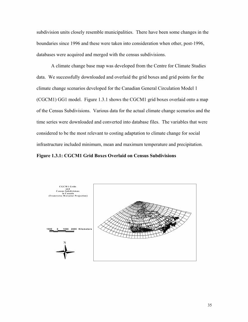
35

subdivision units closely resemble municipalities. There have been some changes in the

boundaries since 1996 and these were taken into consideration when other, post-1996,

databases were acquired and merged with the census subdivisions.

A climate change base map was developed from the Centre for Climate Studies

data. We successfully downloaded and overlaid the grid boxes and grid points for the

climate change scenarios developed for the Canadian General Circulation Model 1

(CGCM1) GG1 model. Figure 1.3.1 shows the CGCM1 grid boxes overlaid onto a map

of the Census Subdivisions. Various data for the actual climate change scenarios and the

time series were downloaded and converted into database files. The variables that were

considered to be the most relevant to costing adaptation to climate change for social

infrastructure included minimum, mean and maximum temperature and precipitation.

Figure 1.3.1: CGCM1 Grid Boxes Overlaid on Census Subdivisions

C G C M 1 G rids an d

C e n s u s S u b d ivis io n s in C a n a d a

(T r a n s ve rs e M er ca tor P r oje ct ion )

1000 0 1000 2000 Kilo m eter s

N

36

Grid boxes are numbered from “1” in the upper left corner (North Pole) to 455

(east of the Maritimes) in the lower right hand corner. In Figure 1.3.1, the last column on

the right has been shortened.

Although cost prohibited their use, digital maps of the Canadian road network are

available. These maps are available as CD ROMs of single 1:50,000 sheets. Detailed

road information could then be overlaid onto the Census Subdivision map and the

CGCM1 climate grid map to arrive at the climate change scenario for each amount of

road kilometrage for each municipality. We could do this kind of detailed work later if

requested to do so.

1.3.6: Codes and Standards

A database of various standards and codes that may be affected by climate change

was compiled. The Canadian Standards Association, Techstreet Publishers, university

libraries and various provincial experts have been utilized as a source of information.

Separate files for international, national and some provincial codes of practice were

assembled. These codes include, but are not limited to, the design, construction and

operation codes for housing, bridges, electrical work, plumbing work and shipping.

Many of these codes and standards have climate factors built into their specifications.

For structures, such as bridges, buildings and roads, the codes and standards are a

reflection of the expected longevity of the structure under a given set of climatic

conditions. The full list of relevant codes and standards for Ontario and Canada has been

compiled. A full list of the codes and standards for roads, bridges and storm water

management systems has been acquired for the country. We examined the standard

codes for many structures and determined what the costs or savings will be under a new

37

climate regime for a specific area in co-operation with cost engineers familiar with the

codes. Codes and standards are particularly important in establishing the costs of new

and replacement structures. Changes in loads, such as occur with wind and snow, and

changes in the substructure, such as occur with permafrost and soil moisture, are

particularly important with buildings and bridges. Thermal expansion is important for

bridges and roads. Drainage and storm runoff, in particular, affect most structures.

Codes and standards for design often do not factor into maintenance costs and these must

be assessed separately. Operating codes may also be involved in the assessment of the

cost of climate change adaptation as climate may alter practices such as ship operation.

1.3.7: Climate Change Factors

We assembled a list of climate change factors that affect adaptation costs. As

stated above, we decided to use the CGCM1, GG1 model for our base, as this model is

highly regarded in the international climate change science community. There are 18

climate change factors that have been modelled by the CGCM1. Other general

circulation models are located at the website of the University of Victoria, Canadian

Institute for Climate Studies. These factors include:

• Mean Annual Temperature • Annual Minimum Temperature • Annual Maximum Temperature • Annual Incident Solar Radiation • Annual Wind Speed • Annual Diurnal Temperature Range • Annual Relative Humidity • Annual Vapour Pressure • Annual Sea Ice • Annual Snow Water • Annual Soil Moisture • Annual Fractional Cloud Cover • Annual Evaporation • Annual Specific Humidity

38

• Annual Precipitation • Mean Annual Sea Level Pressure • Annual Surface Temperature • Annual Potential Evapotranspiration

The CGCM1 model offers climate change scenarios for a base (1961-1990) and

three projected scenarios (2020, 2050, 2080) for the entire country. The data files for

each factor include values for 455 grid boxes for each month of the year, aggregations of

months and an annual total. The information on changes in the climate change factors is

given at a very general level (grid size 3.75 degrees of latitude by 3.75 degrees of

longitude). The 18 variables can be merged with the GIS to give us current and projected

climate change scenarios for grids that vary in size from approximately 130,000 square

km to approximately 15,000 square km. According to the CICS, a finer grid (0.5 degrees

of latitude by 0.5 degrees of longitude) will be ready shortly. This refined grid will be an

interpolation of the existing grid information and will not represent more localized

information on climate change for Canada. Downscaling models are being developed,

but at the moment only one is available. There is evidence that a large amount of

heterogeneity exists within a 3.75 x 3.75 degree unit and downscaling may be necessary

to develop better cost estimates. Downscaling is discussed in Chapter 2.

In addition to the climate factors derived from the CGCM1 model, there are other

factors that we have added where reliable information has been available. These include:

• Sea Level • Inland Water Level • Inland Ice Cover • Atmospheric Carbonation Increase • Frequency of Natural Catastrophes

39

There are additional climatic factors that will change with global warming and

probably should be included in this study. Values for many of these factors can only be

acquired either through interpretation of daily climatic data or as combinations of various

climatic and non-climatic factors. These include:

• Frost-free Period • Amount of Spring Runoff • Frequency of Freeze-Thaw Cycles • Frequency of Wet-Dry Cycles • Intensity of Frost-Heave • Atmospheric Particulates • Water Turbulence • Slope Stability • Seawater Salinity

At present, we do not have a satisfactory means of determining reasonable change

scenarios for many of these factors. Projections for future years for factors that are

derived from daily climatic data, such as freeze-thaw cycles and wet-dry cycles, are not

currently available. There are indications that changes in these factors have already

occurred and may be affecting buildings and other structures (Joan Klaassen,

Meteorological Service of Canada, personal communication).

As reliable climate change scenarios are not available for many factors, we are not

able to determine the size of the range that must be included with each climate change

factor in order to determine its impact. We have used statistical proxies to arrive at

reasonable cost estimates for adaptation to changes in these variables. There are also

indications that cost estimates derived from a general model and cost estimates derived

from a group of regional models for the same area will be substantially different for some

types of adaptation (Linda Mearns, NCAR, Laval workshop presentation). It can be seen

from the downscaling work that is being done, and comparisons of costs that have been

40

conducted from the general climate and the regional climate models, that more

heterogeneity is present at the regional level than at the general level and the difference in

costs derived from the general model base to the regional model base can be substantial.

1.3.8: Statistics Canada Census 1996

Information from the 1996 census for Canada has been acquired as a spreadsheet

and can be attached to the census subdivision map in the GIS. This information includes

such variables as the type of census subdivision (town, county, municipality, etc.)

population, area and number of dwellings. There are 5562 census subdivisions for 1996

and they correspond very closely to municipalities. We used this as a base to compile

information on websites, telephone numbers, addresses and contacts within each census

subdivision (municipality).

It should be noted that there are 8373 polygons in the GIS base map provided by

Statistics Canada. This is because there are census subdivisions that contain several

islands and the GIS software handles each island separately. Spatial analysis may be

complicated because of this.

1.3.9: Municipal Financial Information

We obtained budget information at the municipal (census subdivision) level for

the following provinces and territories:

Ontario, 1997

Alberta, 1997

British Columbia, 1997

Saskatchewan, 1998

Newfoundland, 1996/1997

Manitoba, 1998

41

Nova Scotia, 1997/1998

New Brunswick, 1998

Quebec, 1996

PEI 1999

Northwest Territories 1999

Nunavut – not available

Yukon – not available

The level of detail in this information is fairly broad but does give a breakdown in

municipal costs for such areas of expenditure as roads, sewers and water supply. The

choice of year for budget information may have to vary, as years that involve local

disasters will likely be reflected in government budgets. The year 1998 may not be

appropriate for Ontario or Quebec due to the ice storm in eastern Ontario and western

Quebec. The year 1996 involved flooding and mudslides in parts of Quebec and 1996

and 1997 involved flooding in Manitoba.

The level of information contained in municipal financial statements is fairly

coarse (road expenditures are often rolled up with bridges, ditches and drains) but the

municipal treasurers were consulted for more detail. Regional revenues and expenditures

are included in this information for some provinces. Provincial/territorial budgets for

some provinces/territories were acquired. For many municipalities, the information on

expenditures is broken down by capital and by operating expenses, partly because this is

the required reporting procedure for the provincial accountants and partly because

42

different municipal departments are responsible for capital expenditures and operating

expenditures.

The municipal, regional and provincial budgets provide valuable information for

costing the social infrastructure sector. The codes and standards for the province (and the

country in many cases) provide us with a basis to determine where, and possibly by how

much, the operation and maintenance expenditures may increase or decrease with climate

change, although the codes and standards are more valuable in costing the impact of

climate change adaptation on new structures. This information was incorporated with

questions posed directly to the relevant departments within the government.

1.3.10: Historical Climate Information

An overview account of the climate information for the country has been obtained

for 1997, 1998 and 1999. This information was utilized to establish the general weather

conditions for municipal, regional, provincial and federal financial information. This

information is very coarse but it gives an indication as to whether the expenditures (or

any other information that we gather) for any given year are representative of an average

year climatically. The year 1997, for example, was the 14th warmest for the country in 50

years of data collection; 1998 was the warmest year on record to date.

1.4: Directions for Future Research

During the course of data collection for this sector, it was noted that data

collection could be enhanced for some aspects of the project. These areas included data

that were completely missing or unavailable, data that were inadequate in their scope and

data that were incomplete. These data have been broken down into climate data, census

subdivision data, government financial data and data from other sources.

43

1.4.1: Climate Data

Climate data are fairly complete for basic climate parameters at a coarse spatial

and temporal level. However, for the adaptations and impact research community,

downscaled data at a finer spatial level is required. Downscaling will give more accurate

information spatially. It may be difficult to compensate for the temporal averaging that

characterizes the climate data available for analysis. Daily, and even hourly, data are

necessary in the calculation of the costs of certain climate change adaptations. Culvert

sizes are a prime example. A culvert capacity can be exceeded easily within a few hours

of heavy precipitation. This is equally true for wastewater treatment as shown in Chapter

5. In the end, adaptations must be carried out for extremes. But this information is lost

within monthly, and even daily, averages.

1.4.2: Census Subdivision Data

Census subdivision data are complete for the country for 1996 and could be used

in their present form for another year. A new census is scheduled to begin in June 2001.

Consequently, the old information will not be valid when this information becomes

available. Some census subdivisions could not be sampled since there has been

considerable amalgamation between municipalities in some parts of the country (Ontario

and Quebec, particularly) and it was too difficult to relate costs for the individual

municipalities to the costs for the amalgamated municipalities. Several of the

municipalities involved in amalgamation declined to participate in the survey as they did

not have enough data from previous years to give an estimate of their budget

breakdowns.

1.4.3: Government Financial Data

44

Government financial data were handled at a fairly coarse level. Many of the

activities handled under the operating budget for roads were lumped together, even

though climate may affect these activities differently. Vegetation control will likely have

its own associated climate change costs apart from road maintenance costs. Traffic

signals may also be affected differently from the road surface. These costs were not

treated separately even though other aspects of road maintenance may be affected by

climate change.

Financial information is not complete. While much information was available

online, many municipalities and provinces do not, as yet, provide the level of detail in

expenditures that is necessary to calculate climate change adaptation costs. In addition,

costs are not always aggregated similarly for roads, bridges and storm water

management. While the financial reporting system for the municipalities to the provinces

is fairly consistent, the municipalities do not keep their records for budget allocations in

the same format. The provinces and federal government do not necessarily store their

financial information in the same format either. Many of the questionnaires were

incomplete for this reason and the provincial online information required clarification.

1.4.3.1: Municipal Financial Information

The sample size for municipal financial information was very small; the response

to the questionnaires was not high. More telephone follow up would probably increase

the response. Additional contact information could be acquired and more questionnaires

could be sent out.

1.4.3.2: Provincial Financial Information

45

Provincial financial information is not complete for the country. More

information is required on various capital and operating expenditures relevant for

adaptation costs.

1.4.3.3: Federal Financial Information

Federal financial information was not obtained in detail for road, bridge, storm

water management and winter control expenditures. There are a number of international

“commissions” that are responsible for bridges, such as the Peace Bridge Commission.

These commissions should be contacted separately for future work.

1.4.3.4: Other Government Agencies

Other government agencies that are involved in the construction and maintenance

of social infrastructure include the conservation authorities and other intermediate

government agencies. There are water authorities in Manitoba and, possibly, similar

watershed-based government agencies in a number of provinces. These agencies are

often responsible for major storm water management facilities such as dams. Financial

information from these agencies and data on how many structures are managed was not

acquired.

1.4.4: Other Data Sources

Other data sources, such as the Updated Roads Network provided on CD ROM by

Natural Resources Canada, were not utilized. This digital information would have

facilitated analysis on the roads network as kilometres and types of roads could be

attached to each climate change grid box. Each CD ROM is equivalent to the

information provided on a 1:50,000 National Topographic Service (NTS) sheet. Using a

GIS, this information could have been merged with the census subdivisions, to give an

idea of how many roads of all levels existed within a census subdivision, or merged with

46

the climate change grid boxes to determine how many roads would sustain any particular

climate change.

1.5: Summary

• The fundamental objective was to collect the micro-level data in order to be able

to estimate the costs of adaptation to climate change. This report is restricted to

the costs of adaptation of the road network (roads, bridges, storm water

management systems), and water utilities (drinking water treatment plants, and

wastewater treatment plants).

• For road and water utilities, various databases on current expenditures at the

provincial, municipal and water-utility level were created.

• Time series temperature data from CGCM1, GG1 was downloaded and used to

simulate freeze-thaw cycles and frost heave. For freeze-thaw cycles, oscillations

above and below freezing for each 30-year climate change scenario block were

used as a statistical proxy. For frost heave, the number of months below freezing

was used as a statistical proxy. However, these data need to be validated as no

statistically significant relationships for adaptation costs could be established in

this phase of the work.

• Time series precipitation data from CGCM1, GG1 was downloaded. Experiments

with the downscaling software SDSM were carried out. As SDSM downscaling

can only be done on a limited basis so far, we carried out our own downscaling

for all the sites of water utilities in our sample. Our downscaled data was then

used as the “exogenous shock” in order to simulate the impact of climate change.

47

• There are a number of data gaps that could be filled in at a future date. These data

gaps exist for climate data, census subdivision data, financial data and other types

of data.

48

Chapter 2: Climate Change Projections

As indicated Chapter 1, we have used the scenarios generated by the CGCM1,

GG1, as the exogenous shock representing climate change. The assumption is that if the

climate change scenarios turned out in fact to be real, then the infrastructure under study

would be affected and in order to preserve them as assets, or in order to adapt our capital

assets to the new climatic conditions, some adaptive actions would have to be taken.

Our key variables of climate change for social infrastructure are taken to be

precipitation and temperature. The preliminary question is how the output or projections

of precipitation and temperature in CGCM1 can be made useful, knowing that both the

base year and the projections in the time series portion of the model represent simulated

data. Consider precipitation first as the climatic factor most likely to affect water utilities,

both at the production of drinking water stage and the treatment of wastewater stage.

It has been stated that the CGCM1 projections for precipitation would have to be

downscaled for particular localities. In the next section we describe our learning

experience and our attempts to meet our data needs for projecting climate change and its

impact on water utilities.

2.1: Downscaling Experiment with SDSM

To the best of our knowledge, at the time of writing this report (March 2001) very

little work has been done on downscaling. Canadian Climate Impact Scenarios (CCIS)

group very kindly made some shareware available to use for downscaling. This software

is called Statistical Down Scaling Model (Wilbey et al, 2001), which we shall refer to as

SDSM. In this section we describe our experiments in downscaling, which were done

with the help of Dr Elaine Barrow of CCIS. First, it must be acknowledged that SDSM is

in the early stages of development, and at the time of writing could only do the

49

downscaling for sites contained within the CGCM1 grid box centred on 42.68°N,

78.75°W (this includes Toronto). Another limitation is related to the limited amount of

large-scale observed climate data which was available when SDSM was first developed;

at the moment only 10 years of daily large-scale climate data are available (for the period

1981-1990) and this means that only the corresponding 10 years of daily station data (e.g.

precipitation) can be used in SDSM, regardless of whether a longer station record is

available.

We carried out the experiment in FOUR steps. The first step was to obtain

statistics of the observed precipitation data for Toronto (1981-1990); these were monthly

statistics from daily data on percentage of wet days, the mean, the maximum and

minimum precipitation and its variance. This is shown in Table 2.1.1 given below.

Table 2.1.1: from SDSM: Daily Precipitation Data for Toronto, 1981-1990

50

In step two we carried out multiple linear regression (MLR) equations derived

using observed precipitation data for Toronto and National Centers for Environmental

Prediction (NCEP) reanalysis data (namely the gridded observed data set), providing

large-scale information, with "global" independent variables, such as airflow, F, and

vorticity, Z. In this case eight independent variables were used in the model, since all

eight resulted in the best fit, with the maximum amount of variance explained. The

kurtosis parameter (which describes the distribution of the residuals of the MLR model)

was altered to represent a leptokurtic distribution. The default value in SDSM is 12,

which represents a normal distribution. We replaced it with 60, using trial and error, to

improve the statistics of the synthetic precipitation data so that they more closely

matched the observed statistics. The parameter file obtained when fitting the multiple

linear regression models contains the coefficients for the MLR equations. This parameter

file is used, in conjunction with the independent variables, to generate synthetic

precipitation data for Toronto.

The MLR equations have the form:

Station precipitation = f(independent variables) + error term

If station precipitation generated using the above equation is very close to the

observed statistics in step 1 above, then we are confident that we have derived significant

relationships between the local and large-scale (NCEP data), particularly if the large-

scale (independent) variables explain a large proportion of the variance in station data.

Step 2 indicates the statistics of the station precipitation data that were derived

using the MLR equation above and the NCEP independent variables. The objective is to

check whether the model is working well or not. Ideally we would have used some

51

independent NCEP data to drive the MLR equations, but in this case only data for 1981-

1990 is available, so the same data are being used again. The results are shown in the

Table 2.1.2.

Table 2.1.2: Testing the Toronto Data

The third step is to obtain station precipitation statistics by using independent

variables derived from GCM data for the current baseline period (1961-1990). This gives

an indication of the GCM performance: if the statistics are similar to the observed

statistics, then we can be reasonably "confident" that the relationships between the GCM

independent variables are similar to those of the real data (but see the discussion below).

These are summary statistics of the actual daily output from SDSM using GCM

independent variables for the period 1961-1990. These are shown in Table 2.1.3.

52

Table 2.1.3: SDSM Summary Statistics using GCM Independent Variables

The fourth and final step is to obtain SDSM projections for precipitation for

Toronto for the period 2040-2069. Recall that we used the GCM independent variables

for the 2040-2069 period to drive the MLR equations and to forecast daily precipitation

data for Toronto corresponding to the 2050s period. These are the final summary

statistics for the downscaled scenario. These final results are given in Table 2.1.4

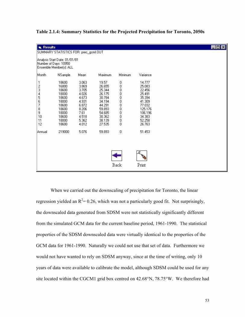
53

Table 2.1.4: Summary Statistics for the Projected Precipitation for Toronto, 2050s

When we carried out the downscaling of precipitation for Toronto, the linear

regression yielded an R2= 0.26, which was not a particularly good fit. Not surprisingly,

the downscaled data generated from SDSM were not statistically significantly different

from the simulated GCM data for the current baseline period, 1961-1990. The statistical

properties of the SDSM downscaled data were virtually identical to the properties of the

GCM data for 1961-1990. Naturally we could not use that set of data. Furthermore we

would not have wanted to rely on SDSM anyway, since at the time of writing, only 10

years of data were available to calibrate the model, although SDSM could be used for any

site located within the CGCM1 grid box centred on 42.68°N, 78.75°W. We therefore had

54

to develop our own methods of downscaling, which are described in Section 2.2. We end

this section by making some observations about SDSM, which might be helpful to the

software developers as they prepare newer releases of SDSM for use by the adaptations

and impact research community. We emphasize that this report is not the place for a full

evaluation or critique of all downscaling methods. We are also aware that some of the

limitations of all downscaling techniques are fully known to the authors of SDSM (see

Wilby et al., 2001). Thus what follows refers exclusively to SDSM.

First, we are not persuaded that the arbitrary trial-and error correction of the

kurtosis parameter is theoretically valid. To support our argument, consider the

following example. A Russian statistician Eugen Slutzky (1937), who made major

contributions to quantitative analysis in economics, took the last two digits of the Russian

lottery and generated from it a time series that “looked” like the fluctuating GDP of the

UK. He had thus generated a time series of business cycles for the UK. The point about

this example is that any time series that merely looks like any other cannot be a proxy for

it. For business cycles it would be legitimate to look at the theory and propose the

governing mechanism of the business cycle (see Dore, 1993). The governing mechanism

will give the model or the set of equations of motion that “govern” the business cycle. In

the case of weather data such as precipitation, we know that the latter is a product of

complex and nonlinear deterministic and stochastic factors acting together. But as

adaptation analysts, we are not competent to claim what the governing mechanism of

precipitation is, and nor are we really interested in it! We want to be able to represent

climate change with a plausible changing distribution of precipitation that is consistent

with other exogenous statistical evidence. We are of the view that the kurtosis parameter

55

that can be changed in SDSM only covers two moments of a given distribution. It would

be good to have software that can capture the moments higher than two. Higher moments

would enable the analyst to experiment with a wider variety of admissible distributions.

Second, in SDSM, the explanatory variables are restricted to physical variables

only, like vorticity and airflow. From our own experience, (see below) dummy variables

representing the months of a year, or the number of seasons, should also be allowed by

the software, since we are concerned with discerning a changing distribution as a result of

climate change.

Third, while recognizing the “low-tech” nature of SDSM based on regression as a

merit, it is unclear to us that the 10-year base is adequate to capture long-term secular

trends in climate change data. Even a 30-year base that we tried showed only a weakly

rising trend in precipitation. It was nevertheless perceptible (see below). And yet it is

clear that even with a long enough base, there must be room for the GCM forcings to

affect the projected scenarios of precipitation for the next 100 years.

Therefore, in the absence of any reliable and usable downscaling of precipitation,

we developed our own proportional downscaling method. It is described in the next

section.

2.2: Proportional Downscaling

As noted above, SDSM utilized a 10-year daily precipitation data time series as

the base, and then the (global) forcing functions project the data for the next three time

slices, 2010 to 2039, 2040 to 2069, and then finally 2070 to 2099. We used a 30-year

base of actual precipitation for 1961 to 1990. We refer to the GCM base as the simulated

base, and use the subscript sb. We replace the GCM base with real and actual

precipitation for 1961 to 1990 and use the subscript rb.

56

In the GCM, let the subscript i represent the year and the subscript m represent the

month; hence pi,m is precipitation in year i in the month m. In addition, let:

gg = greenhouse gases

wv = water vapour

sv = solar variability

ve =volcanic eruptions

ae =aerosols

Then the linearized global forcing functions are:

msbmi paefvefsvfwvfggfp ,54321, )()()()()( +++++= (2.1)

∑=

+•=5

1,, )(

rmsbrmi pfp (2.2)

Next assume that the result of the global forcing is proportional to the simulated

base: i.e.

mimsb

mi

pp

,,

, σ= (2.3)

Then it follows from the proportionality assumption that our projected

downscaled precipitation pp is:

mimrbmi ppp ,,, σ•= (2.4)

In the case studies of water utilities in Chapter 5, we use Equations (2.1) to (2.4)

to generate the downscaled precipitation in which the actual and real base of the

precipitation data for the particular locality is used and equation (2.4) is derived for the

appropriate GCM grid box. Thus for each particular GCM grid box, we utilize the

forcings from that grid box but use the actual and real precipitation data for the base.

57

We accept that the model given in Equation (2.1) to (2.4) is by no means

perfect for proper downscaling. But it shares the “low-tech” property with SDSM. And

yet we found (see below) that the precipitation projections based on that simplified model

yielded plausible results that could be validated by the statistical properties of exogenous

precipitation data.

We are reminded of the dictum:

If you don’t do the best with what you happen to have, you will not do any better with what you should have had!

In fact this dictum is proof by contradiction of Bellman’s Principle of Optimality.

We did not have all the data, because it is not yet available. We did not have time (or the

budget) to study and evaluate all the downscaling. So we followed Bellman’s Principle

in making our downscaled projections.

2.3: Understanding Climate Change

The key question is how do we understand climate change in a concrete sense that

drives adaptation expenditures. We have done a number of statistical experiments with

the projections of the Canadian General Circulation Model (CGCM1), GG1. This

particular CGCM1 experiment can be understood as a particular realization of climate.

Econometricians are wedded to real and actual data, be it for precipitation or

temperature, or anything else. However, a general meta-principle is that even actual data

is only one particular realization. It is a particular realization because it is non-

repeatable. An analogy might help. In chaotic dynamics, if a polynomial governing limit

cycles has an irrational root, we know that even when the governing mechanism is

completely deterministic, the irrational root means that the cycle will never repeat: it will

be unique, like finger prints, or the fractal structure of snow flakes. Thus we propose that

58

most climate patterns are in the final analysis governed by complex nonlinear interactions

among the actual time series, be it precipitation or temperature, and are non-repeating.

Returning to the projections of GCMs, the particular experiment (GG1) of the

particular model (CGCM1) is one possible realization. Therefore actual data has no

greater merit than a possible realization of a GCM experiment, except that actual data

will reflect the statistical properties of a given locality. We could view the GCM

experiment as a possible realization of future climate, but naturally it does not include all

the forcings and feedbacks which occur in the real world, due to modelling constraints

and to our limited knowledge of the forcings and feedbacks. So one could argue that the

actual data has more worth than the GCM data since it does include all these forcings and

feedbacks, although we cannot identify them all. Indeed, if we could, we would be able

to forecast the weather much better and generate future climate with greater confidence.

Thus, it was necessary to use actual data to help with downscaling. In our

experiments, we learned that the GCM projections were "too abstract", representing an

average of a large grid box, and naturally the projections did not reflect the statistical

properties of any particular locality within the grid box. The greater the topographical

diversity of the locality, the greater the departures of the statistical properties of the actual

data from that of the statistical properties of data generated by the GCM experiment. We

found this to be the case for Toronto.

As a result of that finding, we had to "downscale" the projections for all the grid

boxes of interest to us. We showed in Section 2.2 that the downscaling from the SDSM

did not reflect the statistical properties of local Toronto precipitation data. Therefore we

59

carried out our own downscaling. The theory behind our downscaling was described in

Section 2.3.

Having obtained our downscaled projections for Toronto, we set about trying to learn

from this data what the distribution was like and what its properties were. We found that

our own downscaling led to a very plausible realization that seemed to be consistent with

the stylized facts of global warming and the actual data reported by CDIAC. We found

that over future time slices, the mean precipitation was rising slowly, and that the

variance was also increasing. We tried out an ARIMA fit on our downscaled data, in

case the time series was nonstationary. Letting p be the order of autoregressive terms, d

the number of times the data is differenced, and q the order of the moving average terms,

we found that the (p,d,q) of the best model was (1,0,1). This indicated that differencing

was not required (i.e. d= 0), indicating that the projected 100 year time series was

stationary. And yet when we plot the ARIMA fitted values (See Figure 2.3.1), we

observe a slight upward "drift." This reflects the rising means.

Figure 2.3.1: Fitted Values With 95% Confidence Intervals for ARIMA (1,0,0) Model

-3 0 0

-2 0 0

-1 0 0

0

1 0 0

2 0 0

3 0 0

4 0 0

0 1 0 0 2 0 0 3 0 0 4 0 0 5 0 0 6 0 0 7 0 0 8 0 0 9 0 0 1 0 0 0 1 1 0 0 1 2 0 0 1 3 0 0 1 4 0 0

T im e

Tota

l Pre

cipi

tatio

n in

mm

L o w e r C o n f id e n c e L e v e l F i t te d V a lu e U p p e r C o n f id e n c e L e v e l C r i t ic a l V a lu e B a s e M e a n

60

The next question is to suppose our downscaled projections are "valid", i.e. they

are a particular realization, which is at least better and closer to actual data than anything

we might obtain from the GCMs. In that case, how do we understand the changing

distribution of precipitation, a defining characteristic of climate change? As the time

series was stationary and yet there was a perceptible upward drift in the means of the time

slices, we adopted the following linear regression model to bring out the changing

distribution of precipitation. We regressed precipitation on a constant and eleven dummy

variables. The constant "picks up" the January precipitation mean. The coefficient of the

first dummy variable, D1, then yields the marginal contribution of the month of

February, added to the January mean. The coefficient of the second dummy variable, D3,

gives the marginal contribution of the month of March. And so on to December. In this

way, we "see" how the monthly pattern of distribution of precipitation is changing over

the four time slices.

Note that as scientists engaged in the "art of adaptation to climate change", we are

not interested in explaining why the monthly pattern of rainfall is changing; the dummy

variables are not 'explanatory' variables in this sense. For this reason we do not report the

coefficient of variation (R2), which would be meaningless anyway. But we do report the

t statistic for each coefficient. And naturally the overall F statistic for the regression is

significant. To repeat, the objective of the regressions is to see how the monthly pattern

of rainfall is changing. For Welland, for example, we found that climate change means a

wetter spring and a drier summer, followed in the 2040-2079 period with an even wetter

winter! We think that this is a very plausible scenario of climate change.

2.4: Summary and Directions For Future Research

61

In this chapter, the main concern was how to understand and represent climate

change as the required shock in the analysis of this report. We accept that the

precipitation data from the GCM must be downscaled for the particular localities in

which we were interested for estimating adaptation costs. We tried using SDSM for

Toronto. At the time of writing, it was the only locality for which we might be able to

use SDSM for downscaling. However, we found that the resulting downscaled

precipitation did not differ statistically significantly from the GCM simulated base. We

therefore devised our own proportional downscaling model described in equations (2.1)

to (2.4).

The direction for future research here is clear: we need to do experiments with a

number of different downscaling techniques: dynamic downscaling, synoptic weather

typing, stochastic weather generation, and when a new release of SDSM is available, try

regression-based downscaling with the possibility of using dummy variables. Ideally,

trying a number of downscaling methods might help discover whether the projections

converge to some common set, or whether there is a large divergence between them.

62

References:

Dore, M.H.I. (1993). The Macrodynamics of Business Cycles. Malden, Mass and Oxford UK: Basil Blackwell. Slutzky, Eugen (1937). The summation of random causes as the source of cyclical processes. Econometrica 5:105-46. April. Wilby, R.L., Dawson C.W, and Barrow, E.M. (2001). SDSM- a decision support tool for the assessment of regional climate change impacts. Memeo, February 16, 2001 (under review).

63

Chapter 3: The Theory Of The Optimal Production Of Public Goods And Its Application To Social Infrastructure

In economic theory, the roads network and the water utilities (the subject of this

report) would be classified as local public goods, a subclass of public goods. In this

report we shall refer collectively to the road network and the water utility network as

social infrastructure. But it is the service that is provided by social infrastructure that is

the public good, not the capital expenditures. It is the capital assets such as the road

network and the water utility network of a country that provide the flow of services that

are classified as public goods, including local public goods. The costs of adaptation to

climate change can be defined as follows: all expenditures (capital or other) that would be

required for the preservation of the same quality and quantity of services provided by

social infrastructure. In what follows we review very briefly some elements of the

economic theory of public goods to provide the context.

Modern economics defines a pure public good as follows:

1) The use of a good by one consumer does not exhaust the good, so that

others can also "consume" and enjoy its benefits. Furthermore, it is impossible in any

practical sense to charge a user fee or a price for the use of the good. Thus the good is

non-rival and non-excludable in consumption.

2) The cost of producing the good cannot be divided among consumers. If

the cost of the good is indivisible, then its marginal cost – the cost of providing one

additional unit of the good - must be zero.

Standard examples of public goods that meet the above definition are national

defence, flood control, public health programs such as vaccinations and health education.

(See below for other examples).

64

First consider as an example the services of the cable television industry. It is

characterized as follows:

1) It is possible to charge those who derive benefit from the use of the good.

Moreover, those who do not pay can be excluded from the use of the good.

2) The marginal cost – the cost of providing one additional unit of the good -

is positive, and determined by the service and maintenance cost of the extra cable

required to service the area, but probably below its average cost, as the cable companies

are oligopolies.

We can see that the cable TV does not qualify as a public good; it is in fact a

private good. But there are ambiguous examples, such as educational programs for

children and for schools.

Next consider non-commercial broadcasting as an example. Non-commercial

broadcasting is a pure public good. With commercials we have the case that some

beneficiaries can be charged but others cannot. Those who tune in cannot be charged,

and the marginal cost of advertised broadcasting to them is zero. But advertisers can be

charged and those charges cover the costs. The marginal cost of such advertised

broadcasting is positive, not zero.

Somewhere between the two extremes of pure public goods and private goods

falls the case of quasi-public goods. A quasi-public good is characterized as follows:

1) It is difficult and perhaps costly to charge those who benefit from the use

of the good in some or all cases, but some can be charged.

2) The marginal cost of the good is less than the average cost (there are

economies of scale) but it is not zero.

65

Now consider social infrastructure and its services. Social infrastructure can be

considered a quasi-public good. There are economies of scale in the operation of water

utilities and also in the construction and operation of a road network. In the case of the

latter, on some routes it would be feasible to install a mechanism (electronic or other) for

the collection of user fees or tolls. But for most large urban road networks it might be

easier to collect the "tolls" through vehicle licencing, or gasoline taxes. In the case of

water utilities, the installation of water meters makes it simple to charge user fees, and

discriminatory pricing is a widespread practice. Some of these practices in Canada

amount to a subsidy for some large industrial users, with a consequent wasteful use of

water. But to the extent that water is a public good that promotes health, it may not be

wise to cut off water supply to an individual resident who fails to pay. Typically such a

resident's water costs would be covered through some other program.

3.1 The Optimal Quantity of a Public Good

In much of economics, the theory of perfect competition is used as an "ideal"

type, like frictionless space. Under certain specified assumptions, a perfectly competitive

economy results in an optimal allocation of resources. Among the required assumptions

is that the exclusion principle holds, as explained above. That is to say, whether or not a

person consumes a good depends on whether or not he or she pays the price. Those who

pay for the good can consume it, while those who do not pay cannot consume it; that is,

the exclusion principle holds for all consumption goods. Second, it is assumed that the

benefits from a good flow to the particular consumer who has paid the price. Thus, the

consumption of a particular good is rivalrous. If one person consumes a particular good,

someone else cannot consume it as well.

66

But not all goods have both of these characteristics. Goods that do not have the

second characteristic - rivalry in consumption - are called public goods. One person can

enjoy such goods without reducing the enjoyment they give to others, who may not have

paid the price. The classic example is that of the uncrowded bridge. If one individual

crosses the bridge, this does not interfere with another individual’s ability to cross it.

Thus the use of the bridge is a public good.

It is important to note that the market mechanism will not work properly for a

public good even if it conforms to the exclusion principle. For example, in the case of

the uncrowded bridge, it is perfectly feasible to charge a fee for crossing the bridge and to

prevent people who do not pay from crossing it. But it would be inefficient to do so,

since excluding those who do not pay reduces their satisfaction but does not increase the

satisfaction of others. In the economics jargon, it is Pareto inefficient. Thus although the

market mechanism may be applied, it is not optimal to use the market mechanism in

distributing public goods, because to do so is inefficient.

If resources are to be allocated efficiently, what is the socially optimal quantity of

a public good that should be produced? In the case of a private good, under conditions of

perfect competition the optimal output of the private good is at the point where the

marginal benefit each consumer would obtain from an extra unit of the good just equals

the (marginal cost) of providing that good. The market demand for the good is

considered to be the sum of the individual demands. In the case of a public good, the

individual consumers consume the total amount of the good and the combined price paid

by the individual consumers is the sum of the prices paid by each one. That is to say,

optimal output is where the marginal social benefit equals the marginal social cost.

67

Whereas economic efficiency requires that each consumer’s marginal benefit equal

marginal cost for a private good, it requires that the sum of the marginal benefits of all

consumers equal marginal cost for a public good. But when consumers feel that the total

output of the good that will be publicly supplied will not be affected significantly by the

action of any single person, they are likely to make no contribution to producing that

public good. But they will use whatever output of the good is forthcoming, or become

“free riders”. Of course this analysis is of limited use for practical decision making since

individual demand curves will not be revealed.

The answer to the question of the socially optimal output of a public good is

complicated. Public goods are a kind of nonconvexity, and nonconvexities have no

‘interior’ optimal solutions. Frequently, if the public good is produced under conditions

of increasing returns, the social optimum quantity is a “corner solution”: produce as much

of it as is required given the available tax dollars.

3.2 The Changing Nature of a Public Good

There was a time when it was thought that the set of public goods was large:

national defense, health, education, broadcasting, flood control, courts and correctional

facilities, and public utilities such as water, telephones, gas and electricity supply, roads,

and urban transportation were all treated as public goods. Of these, only national

defense, health, education and flood control can still be called "pure" public goods.

Technological change has influenced what was previously considered public goods. For

example, scrambling devices mean that broadcasting is no longer a public good; even the

globally respected BBC Television and Radio are now distributed by private companies.

In Britain, many prisons and correctional facilities have been privatized. While urban gas

pipelines and the telephone wires may be treated as public “utilities” (only one set of

68

pipelines and one set of telephone lines make sense), deregulation has enabled a number

of marketers to use the same hard infrastructure. In the case of telephones, the

development of wireless technology means that there is no justification for thinking of

telephones as a “public utility”, as there can be a number of suppliers of a wireless

telephone service. Electronically detected tolls on roads, such as those on the new 407

ETR in Ontario mean that all publicly provided roads could in principle apply the

exclusion, so that the services provided by roads are no longer pure public goods. In

Britain even water utilities have been privatized.

The private sector is already involved in education in Canada, although education

is a public good in that the benefits of education are not confined to the person who is

educated - there are large social gains from an adequate and well-designed educational

network of schools, colleges, universities and technical institutes. A well-educated and

well-trained labour force benefits private companies as well, and this is well recognized.

The same is true of the public provision of healthcare, as a healthy workforce leads to

fewer lost production days. But in a publicly provided healthcare system, there is a

problem of free riders.

The air traffic control system is clearly a public good, as it makes sense to have

one authority providing the service, because of the nature of the costs, and private

competition in it would be socially harmful. The administration of justice is clearly a

public good, as privatized courts could not dispense justice. Similarly drug safety

regulations cannot be in private hands, and this is also a public good. No technological

developments have affected or changed the nature of these public goods.

69

The key question for any good is always the price that will be charged and the

quantity that will be supplied, if a good is left to the market place. A single private

supplier would supply at a monopoly price by limiting the quantity supplied. That is why

the older privately owned utilities (such as telephone monopolies like Bell Canada and

AT & T in the United States) were subject to a rate of return regulation, and price

increases had to be approved by a regulatory body (the CRTC in Canada and the FCC in

the United States).

In this report we are concerned with social infrastructure, such as roads, bridges

and water utilities as candidates for the title of local public goods. The dividing line

between national and local public goods is not hard and fast. For example, the Trans-

Canada Highway is both a local public good and a national public good, irrespective of

who finances it. Local public goods such as roads and bridges are subject to "congestion"

costs, when inappropriate pricing leads to overuse of a highway, such as the 401. Even

with high gasoline taxes, drivers on the 401 do not pay the "full price" for the operation

of the 401, and a lot of freight that uses the 401 could, from the point of view of society,

be beneficially diverted to the rail network. Unfortunately the tax structure provides a

hidden subsidy to users of the 401, which also puts the railway network at a tax

disadvantage (Eric Reguly, The Globe and Mail, March 17, 2001). However, the subject

of this report is not the question of the socially optimal pricing of highways and water

utilities, although we shall return to that below as a possible adaptation measure. The

question in this report concerns the costs of adapting this infrastructure to climate change.

Traditional economic theory might still be inclined to treat infrastructure as a local public

70

good, and in so far as the road and water network help industry, both have the

characteristic of an intermediate public good, sometimes also called a quasi-public good.

As stated above, the road network belongs to the class of local public intermediate

good. Such a good can be used as an input in production, and the input can be used

simultaneously by a group of firms. Jointness in use prevents the market from extracting

a price from firms unless certain firms can be excluded. But even if they can be

excluded, they ought not to be on efficiency grounds, as argued above. Informational

problems regarding the benefits generated by public intermediate goods are prevalent but

the problems may not be insurmountable. As Musgrave (1959) points out, the benefits of

public intermediate goods may accrue to firms as pure profits or rents and these may be

in principle observable.

As argued above, roads could be considered intermediate public goods or quasi-

public goods, as it does not make sense to provide more than one direct road from point

A to point B. Similarly a water utility is a natural monopoly, with the obvious economies

of scale in production. Therefore its output is also a intermediate public good.

Since there are economies of scale, the marginal cost curve is downward sloping,

and as the marginal cost of the good is less than its average cost, the optimal quantity

cannot be defined. As the optimal quantity cannot be determined, neither can the optimal

price. Thus we are again led to view the optimal solution as a corner solution to a

nonconvex problem.

Another interesting feature is that the nature of a quasi-public good changes if we

introduce a budget constraint in the form of the total allocation given to a local authority

or any other jurisdiction. Suppose that a municipality has a given fixed budget, and is

71

required to fulfill its mandate within the constraints of the budget. Then this becomes a

problem of the theory of the Second Best. In this theory all simple rules, such as pricing

on the basis of marginal costs no longer apply. In this situation, the local authority will

attempt to work out what level of road services, etc. it can supply within the budget and

what prices it will have to charge in order to fulfill its mandate.

3.3 Climate Change and Social Infrastructure

The question of whether social infrastructure is a local public good, a quasi-public

good or an intermediate public good is relevant to the question of whether the services of

the social infrastructure should be publicly provided or whether provision should be left

to the market place. We have argued that when there are nonconvexities, the social

optimum cannot be determined. A fortiori the market place will not be able to provide

those services and there is a prima facie case for public provision. However, once the

social infrastructure exists, these assets must be preserved when damaged by climate

change, whether they are in the private sector domain or in the public domain. It is these

additional costs designed to maintain the integrity of the portfolio of social assets that

must be identified as the costs of adaptation to climate change. Some would argue that as

these adaptation costs would be additional or marginal, the optimal adaptation costs

should be determined by the rule that the marginal costs should just equal marginal

benefits. In our literature review, we have argued against this rule, in part on the ground

that the rule is valid only if we can view climate change as additively separable and

therefore marginal. All the evidence it that climate change is NOT marginal.

Finally, there is mounting evidence (Sturm, 1998) that in all the OECD countries

including Canada, there has been a dramatic decline in public capital expenditure in the

maintenance of all avenues of public concern. Thus in Canada there have been declines

72

in real expenditures in health, education, culture, and in social infrastructure. The quality

of roads has declined, and as the quality of a road declines, it is used less by the public;

the decline in use then enables the authorities to downgrade the classification of the road

and reduce maintenance expenditure even further. With enough time, this downward

spiral can be documented over and over in Canada. The decline in expenditure has also

taken the form of "downloading", i.e. the Federal authorities delegate the responsibility

for roads to the provinces, which in turn download the fiscal responsibility to the regional

authorities, which in their turn download the fiscal responsibility to the municipalities.

Many of the municipalities just do not have the tax base to assume the full financial

burden.

The decline in expenditures partly explains the decline in government regulation

and quality control. There is a strong argument that the Walkerton disaster in Ontario in

2000 could be partly explained by lack of government supervision following drastic cuts

to the budget of the Ontario Ministry of the Environment.

Thus, ideally, the cost of adaptation must be determined on the basis of

maintaining the integrity of the service of social infrastructure. In practice, what the

quality and level of service would have been without this deterioration may not be easy to

establish.

While restoring the integrity of the social infrastructure should form the basis of

estimating the costs of adaptation, it is also clear that some structural reforms would also

help the adaptation process, by reducing the overuse of highways and reducing wasteful

use of water. For roads, Eric Reguly (op. cit.) has argued that rail transportation is five

times more efficient than trucking freight on the highways. Removing the distorting

73

effects of all taxes taken together would reduce freight traffic on some of Canada's

busiest roads and also reduce wear and tear. For water, it has been argued that the

declining water price schedules for large industrial users leads to a wasteful use of water.

Reducing wasteful use would also reduce the costs of wastewater treatment. As Chapter

5 shows, some of the most important adaptation costs faced by water utilities are in the

area of wastewater treatment.

In the two chapters that follow (Chapters 4 and 5) we present our estimates of the

costs of adaptation for the road network and for the case studies of water utilities. Except

when stated, all dollar figures are current 2001 dollars. Throughout this study, no use of

discounting is used. For a justification, see Dore and Burton (2000, Section 2.7 pp39-

46). Furthermore, no assumptions about risk aversion are made.

3.4 Summary and Directions for Future Research

We have argued that social infrastructure is an asset that provides services that

can be called intermediate public goods or quasi-public goods. The quality and quantity

of public infrastructure has declined over the last 25 years in most OECD countries,

including Canada. Adapting this infrastructure to climate change would ideally require

determining the original quality some 25 years ago and then estimating what the costs of

damage due to climate change would be. In practice this may not be possible. The best

we can hope for is to estimate the costs of adaptation that restores the integrity of the

services provided by the infrastructure. However those costs that can be attributed

directly to climate change must be included.

Some directions for future research include:

Measures of adaptation to climate change should also include "demand

management", whereby existing distortions in the structure of fuel prices, property and

74

other taxes lead to overuse of highways and underuse of the rail network. A proper study

could identify which taxes are distortionary and what tax structure would be equitable so

that the rail sector is not disadvantaged. This should be part of the National

Transportation Strategy that is now being developed.

The pricing policy of water should encourage conservation and reduce wasteful

usage of water. The differential impacts of different water pricing policies should be

studied. A good beginning would be to eliminate the declining price schedules faced by

large industrial users.

75

References: Dore, M.H.I. and Burton, I (2000). The Costs of Adaptation to Climate Change: A Critical Review, November 15, 2000.

Musgrave, R. (1959). The Theory of Public Finance. New York: McGraw-Hill.

Reguly, Eric (2001). "Ontario backs transfer of wealth from taxpayer to the trucker," The Globe and Mail, Saturday, March 17.

Sturm, Jan-Egbert (1998). Public expenditure in OECD countries: the causes and impact of the decline in public capital spending. Cheltenham UK, and Northampton, Mass: Edward Elgar.

76

Chapter 4: Roads and Bridges in Canada

This chapter deals with the main impacts of climate change on road infrastructure

and the required adaptation costs. We have broken the road system into its three main

components: roads, bridges and storm water management systems. We suggest that the

main impacts of climate change will be different for each of these components. For

roads, the main impact will be on (a) operating costs such as road repair and winter

control and on (b) capital costs to replace temporary winter/ice roads with permanent

roads and replace roads on permafrost. For bridges, the main impact will be on (a)

capital costs to replace coastal bridges and (b) operating costs for changes in road salt

application. Storm water management systems are a small component of the overall costs

for the road network. The direct impact of climate on the storm water management

system is small; the indirect effect of road washouts is much larger but requires

assessment in terms of the frequency of heavy precipitation. Section 4.1 gives an

introduction; Section 4.2 gives basic climate information and Section 4.3 covers the

jurisdiction of roads, bridges and storm water management systems in the country.

Section 4.4 covers the design codes and standards for road, bridge and storm water

management design. Section 4.5 provides details of the major components of costs and

their associated climate factors and Section 4.6 gives the costs of adaptation. The chapter

ends with suggestions for directions for future research and a comprehensive summary of

the material covered in the chapter.

4.1: Introduction

There are 900,000 to one million km of roadways in Canada and the expenditures

exceed $1 billion Canadian per year to maintain, upgrade, replace and build roadways.

The road transportation system moves 90% of the Canadian populace and 70% of freight

77

by revenue (PaulDeLannoy, MSC, personal communication).

The road system in Canada can be broken into several components, all of which

would be expected to sustain different levels of climate impact and would incur different

costs of climate adaptation. Roadways consist of roads, bridges and a drainage system

(ditches and drains). Bridges are special structures to carry roadways over various

impediments. The drainage system includes both existing waterways and the runoff from

the roadway itself. Bridges and culverts may be included as part of the drainage system.

The structures and practices associated with roadways have two purposes:

1) Provide safe use of the roadway

2) Ensure the longevity of the road system

These two purposes are often at odds with one another. Safety provisions, such as

the application of more than 4.7 million metric tonnes of salt yearly (Paul DeLannoy,

MSC, personal communication) has a tremendous impact on the longevity of some of the

components of the roadway. Safe stopping distances must be maintained, but at a price.

Concrete structures (bridges are a prime example) are subject to greater breakdown due

to salt application. Bridges not only deteriorate due to salt but, due to increased

susceptibility to icing, are also more heavily salted. Climate factors heavily into salt

application. Salt is applied to roadways under very specific climatic conditions (below

freezing but above –10 degrees C). Federal, provincial, regional and municipal

governments are constantly working to balance their capital costs for replacement of

existing structures against the costs of maintenance for deterioration of these structures

and maintenance for safe operation. In addition, there is wear and tear on roadways from

traffic and from climate itself. Roads must be kept free of potholes in order to allow safe

78

driving and the concrete spalling on bridges must be repaired to prevent deterioration of

the rebar that provides strength and integrity to the structure. Ditches and drains must be

maintained to allow precipitation to flow off the roadway and not become a hazard to

driving. They must be designed to handle even rare events; otherwise the structure of

the roadway and its safety may be compromised.

Roads, bridges and storm water management systems are designed and

constructed at the federal, provincial or territorial, regional (if it exists) and municipal

level in Canada. Each level of government has its own road system with associated

bridges and storm water management system. Although these systems are usually

distinct, there may be some overlap in terms of cost sharing for maintenance or

construction. The various levels of government recognize that a single road may carry

benefit for transportation locally, regionally, provincially/territorially and nationally. All

provinces and territories have roads and bridges that are federally maintained,

provincially/territorially maintained and municipally maintained. In some provinces, a

regional level of government exists as well, but this is not consistent across the country.

The disparity in government structure across the country has resulted in very different

distributions of responsibilities for road and bridge construction and maintenance across

the country. A very different picture of road and bridge construction and maintenance

has emerged as a result. In addition, different codes and standards for roads, bridges and

storm water management system construction are in place across the country. Most

municipalities and regions follow the provincial standards for road and bridge

construction; no federal standard currently exists for road, bridge or storm water

management system construction. Municipalities and regions are not required to follow

79

these standards, but they usually do. The more populous municipalities usually employ

their own engineers; the less populous municipalities usually employ engineering firms to

do the design and construction for them. Maintenance procedures for roads, bridges and

storm water management systems are fairly consistent across the country.

4.2: Basic Climate Information

Global warming will benefit winter transportation in most parts of Canada.

Reduced winter snowfall will reduce snow removal, salt/sand application and road

maintenance in much of southern Canada. However, the risk of increased freezing rain

conditions in winter could pose a problem. Melting permafrost in northern areas could

also pose transportation problems since the ground must be frozen to allow unrestricted

travel. This could shorten the land transportation season in the North and increase costs

(Environment Canada, http://www.ec.gc.ca/climate/primer/sec-6.htm#12).

Overall, there will likely be a loss of extreme temperatures and less impact on all

structures. Climate change appears to be resulting in a loss of the lows but not

necessarily gains of higher temperatures (Phil Jarrett, Environment Canada, personal

communication). There may be changes in the number of freeze-thaw cycles. A change

in freeze-thaw cycles is more likely to occur in the heartland with fewer cycles on the

west coast (PaulDeLannoy, MSC, personal communication). An overall increase of

approximately 5°C is expected to occur, accompanied by an increase of approximately

10% in precipitation. Sea level is expected to rise by approximately one metre, due to the

melting of the ice cap but more recent research indicates that the rise may be less in the

northern latitudes, as the gravitational pull of the ice caps is reduced.

4.3: Roads, Bridges and Storm Water Management Jurisdiction in Canada

80

There are currently 2,400 km of roads under federal jurisdiction in Canada. There

are also 33 bridges and tunnels throughout the country that are maintained by the federal

government. The national highway system includes 24 international crossings, roads and

bridges under Parks Canada, roads and bridges under Public Works Canada, roads and

bridges under the National Capital Commission and roads maintained by the Department

of Indian and Northern Affairs. The federal government also contributes to the provincial

highway system (Transport Canada,

http://www.tc.gc.ca/pol/en/Report/Highway_Historical _Look/Chapter2.htm).

The provincial and territorial governments are responsible for most of the main

thoroughfares in the country. The distribution of roads and bridges between the

provincial and local governments is quite variable across the country (Table 4.3.1 and

Table 4.3.2). In Ontario, the regional government assumes many of the responsibilities

for road, bridge and storm water management system construction that would otherwise

be handled by the province. Other provinces, such as British Columbia, also have a two-

tier local government system. Both the municipal and regional levels of government

handle roads.

81

Table 4.3.1: Road Jurisdiction in Canada (2-lane equivalent) Province/Territory Federal Roads

(km) Provincial Roads (km)

Municipal Roads (including Regional) (km)

Total Roads (km)

Alberta 4,076 (3,973) 18,767 (18,292) 163,307 (159,172) 186,150 (181,437) British Columbia 2,626 (2,050) 54,161 (42,279) 27,413 (21,399) 84,200 (65,728) Manitoba 2,784 (1,740) (21,628) (64,500) (87,868) New Brunswick 400 (219) 21,300 (18,480) 3,671 (3,185) 25,371 (21,884) Newfoundland 500 (207) 9,000 (8,747) 4,246 (4,127) 13,746 (12,081) Nova Scotia 500 (291) 26,000 (23,371) 2,592 (2,330) 29,092 (25,992) Ontario 4,939 (2,346) (28,458) (137,087) (167,891) Prince Edward Island 100 (57) 5,660 (5,128) 554 (502) 6,314 (5,687) Quebec 2,536 (534) 70,000 (29,344) 92,000 (90,000) 164,536 (119,878) Saskatchewan 3,939 (3,181) 32,441 (26,200) 213,620 (172,522) 250,000 (201,903) Northwest Territories 800 (351) 4,400 (3895) 813 (720) 6,013 (4,966) Nunavut 200 (39) (412) (70) (521) Yukon 600 (94) (4,696) (278) (5,487) Total 24,000 (15,082) (230,930) (655,892) (901,904) Figures in bold are actual numbers for 2000. Figures in brackets are numbers for 1995. All other figures are estimates. AB http://www.gov.ab.ca/aboutalberta/index.cfm BC Annual Report 1999-2000 pg17 NB http://www.gov.nb.ca/dot/mt/maint.htm NF Gary Goss, Newfoundland Works, Services and Transportation, personal communication NS http://www.gov.ns.ca/tran/whoweare/tpwglance.stm PE Helen Blake, Prince Edward Island Transportation and Public Works, personal communication PQ http:www.mtq.gouv.qc.ca/regions SK http://www.touryorkton.com/about_body.html ( ) Bracketed data are for 1995; other data are for 2000. The 1995 data are from following sources: Transportation Association of Canada (TAC), “Transportation in Canada: A Statistical Overview”, 1995 “Canada’s Roadway Infrastructure: Selected Facts and Figures”, 1990 “Highways in Canada 1991 Report” Road and Transportation Association of Canada, Roadway Infrastructure Study, 1987 (updated 1999)

82

Table 4.3.2: Bridge Jurisdiction in Canada* Province/Territory Provincial Bridges

(number)

Municipal Bridges (including Regional) (number)

Total Bridges (number)

Alberta 3,800 8,700 12,500 (>1.8m) British Columbia 3,000 500 3,500 Manitoba 2,400 5,800 8,200 (>2m) New Brunswick 2,800 150 (est) 2,950 (>3m) Newfoundland 1,900 100 2,000 (>6m) Nova Scotia 3,540 280 (est) 3,820 Ontario 2,600 10,000 12,600 (>3.5m) Prince Edward Island 1,200 50 1,250 Quebec 4,700 3,800 8,500 (>4.5m) Saskatchewan 950 100 1,050 Northwest Territories 47 3 51 Nunavut 10 0 10 Yukon 100 1 100 Total 27,047 29,484 56,531 *There are an additional 33 bridges and tunnels maintained by the federal government AB Alan Kwan, Alberta Infrastructure, personal communication BC Bill Szeto, British Columbia Ministry of Transportation and Highways, personal communication MB Wayne Kapar, Manitoba Highways and Transportation, personal communication NB http://www.gov.nb.ca/dot/mt/maint.htm including causeways NF Peter Lester, Newfoundland Works, Services and Transportation, personal communication (exclusive of causeways) NS http://www.gov.ns.ca/tran/whoweare/tpwglance.stm ON David Lai, Ontario Provincial Ministry of Transportation, personal communication PEI Ken Hoy, Prince Edward Island Transportation and Public Works, personal communication PQ http:www.mtq.gouv.qc.ca/regions SK Howard Yee, Saskatchewan Highways and Transportation, personal communication NT Larry Purcka, Northwest Territories Transportations, personal communication NA Doug Sitlin,, Nunavut Community and Transportation, personal communication YK Bernie Cross, Yukon Community and Transportation Services, personal communication Canadian federal government (http://www.tc.gc.ca/pol/en/Report/Highway_Historical _Look/Chapter2.htm).

Roads and bridges may be municipal, regional, provincial or federal. The federal

bridges are often under the jurisdiction of separate bridge commissions. There are 24

international crossings (bridges or tunnels) under federal jurisdiction. The federal

government also owns four intraprovincial bridges, Arthur Laing, Dinsmore (Vancouver),

Jacques Cartier and Champlain (Montreal via the St.Lawrence Seaway Authority). The

83

federal government operates the roadway portion of the Victoria Jubilee (Montreal).

Through the St.Lawrence Seaway Authority, the federal government owns and operates

the Thousand Islands International Bridge (Gananoque), Seaway International Bridge

(Cornwall), Beauharnois Tunnel and the St.Louis and Larocque Bridges over the

Beauharnois Canal (Valleyfield) and the Townline Tunnel (Welland). Blue Water Bridge

Authority (federal) owns the Canadian half of a toll bridge between Point Edward (near

Sarnia) and Port Huron (MI) (Transport Canada,

http://www.tc.gc.ca/pol/en/Report/Highway_Historical _Look/Chapter2.htm).

In Ontario, the province downloaded a number of bridges to the regions in 1997

and the regions subsequently downloaded a number of bridges to the municipalities in

2000. Following the downloading, several Ontario municipalities have indicated that

their bridges may not be in good condition. Some municipalities have posted low load

designations rather than rehabilitate or replace their deteriorated bridges. The jurisdiction

for a bridge, in most cases, follows the jurisdiction for the associated road (i.e. a bridge

on a municipal road is considered to be a municipal bridge).

4.4: Roads, Bridges and Storm Water Management System Design Codes and Standards

The design of roads, bridges and storm water management systems (ditches and

drains) varies across the country. Bridges are more consistent in their design standards,

roads are fairly consistent but storm water management standards are quite variable,

province-by-province. Municipalities are not necessarily required to follow the

provincial guidelines but, as many regions and municipalities hire consulting engineers to

design their roadways, the provincial standards would be expected to reflect the standards

for all roads, bridges and storm water management systems within each provincial

84

boundary. Consulting engineers normally follow accepted provincial practice in order to

avoid the issue of liability should there be a problem with their structure in the future.

Bridge design standards are fairly consistent across the country at present and, with the

completion of the new Canadian Highway Bridge Design Code (CHBDC), will be

uniform for all Canadian bridges in the near future. The CHBDC, which has utilized the

Ontario Highway Bridge Design Code (OHBDC) will replace all existing Canadian codes

including the current CHBDC, CSA Standard CAN/CSA-S6-88, Design of Highway

Bridges, its supplement, CAN/CSA-S6S1-1990, Existing Bridge Evaluation, to CSA

Standard CAN/CSA-S6-88, Design of Highway Bridges and the commentary S6.1-

M1990.

This does not imply that all bridges will adopt the same design, but that the

consideration for different factors, including climatic load factors, will be standard.

Bridges are large, expensive and (usually) long-lived structures. The results of a bridge

failure may be catastrophic, in terms of loss of life and property damage. Consequently,

bridges are designed both carefully and consistently in order to avoid this occurrence.

The current standards for bridge design and construction are intended to provide a

minimum of 50 years’ life for a bridge. In fact, most bridges last much longer. The new

standards that will become effective with the revised CHBDC (currently undergoing the

approval process) are directed toward a 75-year minimum life expectancy. Most of the

improvements in longevity are through improvements in materials, many of which have

been designed to resist or avoid the effects of de-icing road salt, a major cause of the

deterioration of bridges.

85

Roadways are fairly consistent in their design standards as well. Most provinces

use the Transportation Association of Canada (TAC) Geometric Design Guide for

Canadian Roads. There are also guides specific to each province, which often exist to

accommodate special considerations for climate within the province. Alberta and

Saskatchewan have their own guides and Manitoba utilizes the US guidelines in addition

to the TAC guide. Roads are often classified by traffic volume and speed and the design

follows these classifications. Pavement surfaces are fairly specialized and undergoing

constant change, often due to advances in surfacing materials. With pavement surfaces,

the ability to handle high traffic volumes (durability of surface) may be compromised by

adaptation to higher temperature (less viscous binders). Roads are currently designed to

last between 15 and 25 years. The lifespan of a road does not appear to vary much across

the country. Much of the difference in longevity between any two roads may be related

to traffic volumes.

Storm water management is not standardized across the country and probably

reflects the different population densities, history of flooding and normal precipitation for

each province. Some provinces have periodic flooding in areas of high population

density and have made provision, at least in these areas, for these occurrences. The storm

water management systems are usually integrated with bridge and culvert design and with

any flood control structures, such as dams and dikes, in these areas. If this practice were

not followed, then a storm water management system associated with a highway could

potentially compromise the effectiveness of a dam or dike.

4.4.1: Roads

Road design usually follows the Transportation Association of Canada Geometric

Design Guide for Canadian Roads. Other standards, such as the American Association of

86

State Highway and Transportation Officials (AASHTO) “Green Book” are also used.

Some provinces have developed their own guides in order to adapt the TAC guide to their

specific weather and traffic considerations. Construction practices for each type of road

are different. Some provinces have a higher percentage of one type of road than another.

Different road types are not evenly distributed across the country (Table 4.4.3).

Table 4.4.3: Road Type Distribution in Canada (1995) Type Total Km Percentage Freeway 16,571 1.84 Paved 301,348 33.41 Gravel 442,408 49.05 Treated 69,292 7.68 Earth 66,829 7.41 Other 5,455 0.61 Total 901,903 100 Transportation Association of Canada (TAC), “Transportation in Canada: A Statistical Overview”, 1995 “Canada’s Roadway Infrastructure: Selected Facts and Figures”, 1990 “Highways in Canada 1991 Report” Road and Transportation Association of Canada, Roadway Infrastructure Study, 1987 (updated 1999) 4.4.1.1: Alberta

Alberta provincial transportation design engineers usually use Transportation

Association of Canada (TAC) Geometric Design Guide for Canadian Roads for the

structure of the roadway. They also utilize the Alberta publication, “Highway Geometric

Design Guide”. This guide also takes Alberta weather into consideration for structural

aspects of road design. In Alberta it was discovered, for instance, that the super-elevation

on curves was too high for Alberta winter conditions. Rather than using a super-

elevation of 8%, a 6% increase in elevation around the outside of curves has been

stipulated (Peter Ho, Alberta Infrastructure, personal communication). Highways are

expected to last approximately 50 years in Alberta (1999/2000 Annual Report, Alberta

Infrastructure, pg84), although the lifespan of the pavement may be considerably less.

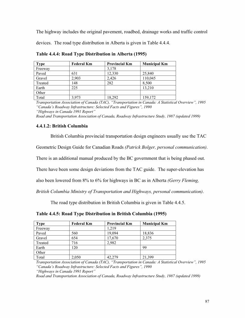
87

The highway includes the original pavement, roadbed, drainage works and traffic control

devices. The road type distribution in Alberta is given in Table 4.4.4.

Table 4.4.4: Road Type Distribution in Alberta (1995) Type Federal Km Provincial Km Municipal Km Freeway 3,178 Paved 631 12,330 25,840 Gravel 2,903 2,426 110,045 Treated 148 282 8,500 Earth 225 13,210 Other Total 3,973 18,292 159,172 Transportation Association of Canada (TAC), “Transportation in Canada: A Statistical Overview”, 1995 “Canada’s Roadway Infrastructure: Selected Facts and Figures”, 1990 “Highways in Canada 1991 Report” Road and Transportation Association of Canada, Roadway Infrastructure Study, 1987 (updated 1999) 4.4.1.2: British Columbia

British Columbia provincial transportation design engineers usually use the TAC

Geometric Design Guide for Canadian Roads (Patrick Bolger, personal communication).

There is an additional manual produced by the BC government that is being phased out.

There have been some design deviations from the TAC guide. The super-elevation has

also been lowered from 8% to 6% for highways in BC as in Alberta (Gerry Fleming,

British Columbia Ministry of Transportation and Highways, personal communication).

The road type distribution in British Columbia is given in Table 4.4.5.

Table 4.4.5: Road Type Distribution in British Columbia (1995) Type Federal Km Provincial Km Municipal Km Freeway 1,219 Paved 560 19,094 18,836 Gravel 654 17,670 2,375 Treated 716 2,982 Earth 120 99 Other Total 2,050 42,279 21,399 Transportation Association of Canada (TAC), “Transportation in Canada: A Statistical Overview”, 1995 “Canada’s Roadway Infrastructure: Selected Facts and Figures”, 1990 “Highways in Canada 1991 Report” Road and Transportation Association of Canada, Roadway Infrastructure Study, 1987 (updated 1999)

88

4.3.1.3 Manitoba

Manitoba provincial transportation design engineers use the TAC Geometric

Design Guide for Canadian Roads supplemented with the American Association of State

Highway and Transportation Officials (AASHTO) “Green Book” Design of Highways

and Streets. The classification of the roadway determines what storm water management

considerations are put in place (Eric Christiansen, Manitoba Highways and

Transportation, personal communication). The road type distribution in Manitoba is

given in Table 4.4.6.

Table 4.4.6: Road Type Distribution in Manitoba (1995) Type Federal Km Provincial Km Municipal Km Freeway Paved 99 7,915 3,225 Gravel 1,358 6,212 61,275 Treated 10 4,720 Earth 273 Other 1,640 Total 1,740 21,628 64,500 Transportation Association of Canada (TAC), “Transportation in Canada: A Statistical Overview”, 1995 “Canada’s Roadway Infrastructure: Selected Facts and Figures”, 1990 “Highways in Canada 1991 Report” Road and Transportation Association of Canada, Roadway Infrastructure Study, 1987 (updated 1999) 4.4.1.4: New Brunswick

New Brunswick provincial transportation design engineers use the TAC

Geometric Design Guide for Canadian Roads (Neil Gilbert, New Brunswick Department

of Transportation, personal communication). The road type distribution in New

Brunswick is given in Table 4.4.7.

89

Table 4.4.7: Road Type Distribution in New Brunswick (1995) Type Federal Km Provincial Km Municipal Km Freeway 494 Paved 89 4,393 2,263 Gravel 94 4,730 Treated 26 8,863 922 Earth 10 Other Total 219 18,480 3,185 Transportation Association of Canada (TAC), “Transportation in Canada: A Statistical Overview”, 1995 “Canada’s Roadway Infrastructure: Selected Facts and Figures”, 1990 “Highways in Canada 1991 Report” Road and Transportation Association of Canada, Roadway Infrastructure Study, 1987 (updated 1999) 4.4.1.5: Newfoundland

Newfoundland uses the TAC Geometric Design Guide for Canadian Roads

(Garry Goss, Newfoundland Works, Services and Transportation, personal

communication). The road type distribution in Newfoundland is given in Table 4.4.8.

Table 4.4.8: Road Type Distribution in Newfoundland (1995) Type Federal Km Provincial Km Municipal Km Freeway 110 Paved 162 6,393 3,116 Gravel 32 2,241 1,011 Treated 2 Earth 11 Other Total 207 8,747 4,127 Transportation Association of Canada (TAC), “Transportation in Canada: A Statistical Overview”, 1995 “Canada’s Roadway Infrastructure: Selected Facts and Figures”, 1990 “Highways in Canada 1991 Report” Road and Transportation Association of Canada, Roadway Infrastructure Study, 1987 (updated 1999) 4.4.1.6: Nova Scotia

Nova Scotia provincial transportation design engineers use the TAC Geometric

Design Guide for Canadian Roads (Tom Gouthro, Nova Scotia Transportation and Public

Works, personal communication). The road type distribution in Nova Scotia is given in

Table 4.4.9.

90

Table 4.4.9: Road Type Distribution in Nova Scotia (1995) Type Federal Km Provincial Km Municipal Km Freeway 1,518 Paved 141 12,377 2,209 Gravel 108 9,476 121 Treated 0 Earth 42 Other Total 291 23,371 2,330 Transportation Association of Canada (TAC), “Transportation in Canada: A Statistical Overview”, 1995 “Canada’s Roadway Infrastructure: Selected Facts and Figures”, 1990 “Highways in Canada 1991 Report” Road and Transportation Association of Canada, Roadway Infrastructure Study, 1987 (updated 1999) 4.4.1.7: Ontario

Ontario provincial transportation design engineers use the TAC Geometric Design

Guide for Canadian Roads. The primary road-building design guide in Ontario is the

provincial publication, Geometric Design Standards for Ontario Highways, which was

last updated in 1994 (Michael Thomas, personal communication). Some modifications

have been made to the TAC standard, including a reduction in the super-elevation from

8% to 6% for most roads. In Ontario, only roads that will have high levels of de-icing

chemicals applied on a regular basis will have the higher super-elevation level built into

the road (Darsham Bhatia, Ontario Ministry of Transportation, personal

communication). Pavement lasts approximately 15 years in Ontario, if properly

maintained (Ontario Ministry of Transportation,

http://www.mto.gov.on.ca/english/about/quickfacts.htm). The road type distribution in

Ontario is given in Table 4.4.10.

91

Table 4.4.10: Road Type Distribution in Ontario (1995) Type Federal Km Provincial Km Municipal Km Freeway 3,868 Paved 343 20,418 47,965 Gravel 1,308 900 60,225 Treated 271 3,272 25,550 Earth 424 3,236 Other Total 2,346 28,458 137,087 Transportation Association of Canada (TAC), “Transportation in Canada: A Statistical Overview”, 1995 “Canada’s Roadway Infrastructure: Selected Facts and Figures”, 1990 “Highways in Canada 1991 Report” Road and Transportation Association of Canada, Roadway Infrastructure Study, 1987 (updated 1999) 4.4.1.8: Prince Edward Island

Prince Edward Island provincial transportation design engineers use the TAC

Geometric Design Guide for Canadian Roads. Roads have a 15 to 25 year life span in

Prince Edward Island (AlAiken, Prince Edward Island Transportation and Public Works,

personal communication). The road type distribution in Prince Edward Island is given in

Table 4.4.11.

Table 4.4.11: Road Type Distribution in Prince Edward Island (1995) Type Federal Km Provincial Km Municipal Km Freeway Paved 41 3,618 502 Gravel 8 254 Treated 0 Earth 8 Other Total 57 5,128 502 Transportation Association of Canada (TAC), “Transportation in Canada: A Statistical Overview”, 1995 “Canada’s Roadway Infrastructure: Selected Facts and Figures”, 1990 “Highways in Canada 1991 Report” Road and Transportation Association of Canada, Roadway Infrastructure Study, 1987 (updated 1999)

4.4.1.9: Quebec

Quebec provincial transportation engineers use their own standards for road

design. These standards were developed within the province (Darsham Bhatia, Ontario

Ministry of Transportation, personal communication). The road type distribution in

92

Quebec is given in Table 4.4.12.

Table 4.4.12: Road Type Distribution in Quebec (1995) Type Federal Km Provincial Km Municipal Km Freeway 4,707 Paved 294 22,231 66,000 Gravel 194 2,406 24,000 Treated 6 Earth 40 Other Total 534 29,344 90,000 Transportation Association of Canada (TAC), “Transportation in Canada: A Statistical Overview”, 1995 “Canada’s Roadway Infrastructure: Selected Facts and Figures”, 1990 “Highways in Canada 1991 Report” Road and Transportation Association of Canada, Roadway Infrastructure Study, 1987 (updated 1999) 4.4.1.10: Saskatchewan

Saskatchewan provincial transportation design engineers use the TAC Geometric

Design Guide for Canadian Roads. This guide is augmented with Saskatchewan’s own

design manual. Saskatchewan has many roads of low traffic volume, which must be

designed for high speed, the cold conditions and snowfall. The terrain is also very flat.

There are four classifications of roads in Saskatchewan. Roads are generally designed to

last approximately 15 years. The temperature range in Saskatchewan is very high and is

hard on the durability of roads but the traffic volumes are usually fairly low (SukhyKent,

Saskatchewan Highways and Transportation, personal communication). The road type

distribution in Saskatchewan is given in Table 4.4.13.

Table 4.4.13: Road Type Distribution in Saskatchewan (1995) Type Federal Km Provincial Km Municipal Km Freeway 49 Paved 80 11,525 8,021 Gravel 2,281 5,847 116,600 Treated 19 8,729 2,175 Earth 801 45,700 Other 50 Total 3,181 26,200 172,522 Transportation Association of Canada (TAC), “Transportation in Canada: A Statistical Overview”, 1995 “Canada’s Roadway Infrastructure: Selected Facts and Figures”, 1990 “Highways in Canada 1991 Report”

93

Road and Transportation Association of Canada, Roadway Infrastructure Study, 1987 (updated 1999) 4.4.1.11: Northwest Territories

In the Northwest Territories, road design engineers use the TAC Geometric

Design Guide for Canadian Roads. The road surface in the Northwest Territories may

last 15 years, which is comparable to the rest of the country. The roadbed itself often has

a shorter lifespan, though, than the rest of the country. Due to the problems with high

soil water content and permafrost changes, roadbeds in the Northwest Territories may

only last 25 years. Roadbeds in other parts of the country will last up to 50 years. The

Alberta provincial road design guide is also used (Larry Purcka, Northwest Territories

Transportation, personal communication). The Northwest Territories is very dependent

upon temporary winter roads for transportation. The road type distribution in the

Northwest Territories is given in Table 4.4.14. These figures have been adjusted for the

change in road jurisdiction that occurred when the territory of Nunavut was formed. All

of the paved roads are found within the Northwest Territories. Approximately 90% of

the other types of roads remained within the Northwest Territories after the creation of

the territory of Nunavut (Larry Purcka, Northwest Territories Transportation, personal

communication).

Table 4.4.14: Road Type Distribution in Northwest Territories (1995) Type Federal Km Territorial Km Municipal Km Freeway Paved 0 187 90 Gravel 296 1492 630 Treated 0 322 Earth 55 Other 1894 Total 351 3895 720 Transportation Association of Canada (TAC), “Transportation in Canada: A Statistical Overview”, 1995 “Canada’s Roadway Infrastructure: Selected Facts and Figures”, 1990 “Highways in Canada 1991 Report” Road and Transportation Association of Canada, Roadway Infrastructure Study, 1987 (updated 1999)

94

4.4.1.12: Nunavut

There is no standard for road construction in Nunavut. There are no hard-

surfaced roads; all roads are graveled (Doug Sitlin, Nunavut Community and

Transportation, personal communication). The road type distribution in Nunavut is

unavailable for 1995, as Nunavut was part of the Northwest Territories at that time.

According to Doug Sitlin, all roads are gravel in Nunavut. According to Larry Purcka

(Northwest Territories Transportation, personal communication) the division of roads

between the Northwest Territories and Nunavut was approximately 9:1 (90% of the roads

remained under the jurisdiction of the Northwest Territories after Nunavut separated).

An approximation of the road distribution in Nunavut is given in Table 4.4.15.

Table 4.4.15: Road Type Distribution in Nunavut (1995) Type Federal Km Territorial Km Municipal Km Freeway Paved 0 0 0 Gravel 33 166 70 Treated 0 36 Earth 6 Other 210 Total 39 412 70 Derived from Northwest Territory figures

4.4.1.13: Yukon

Design engineers in the Yukon utilize the TAC Geometric Design Guide for

Canadian Roads (Bernie Cross, Yukon Community and Transportation Services, personal

communication). The road type distribution in the Yukon is given in Table 4.4.16.

95

Table 4.4.16: Road Type Distribution in Yukon (1995) Type Federal Km Territorial Km Municipal Km Freeway 3 Paved 0 263 94 Gravel 86 2,744 137 Treated 8 1,686 47 Earth 0 Other Total 94 4,696 278 Transportation Association of Canada (TAC), “Transportation in Canada: A Statistical Overview”, 1995 “Canada’s Roadway Infrastructure: Selected Facts and Figures”, 1990 “Highways in Canada 1991 Report” Road and Transportation Association of Canada, Roadway Infrastructure Study, 1987 (updated 1999) 4.4.2: Bridges

Bridges are structures that vary in definition across the country. Bridges may

include culverts and range in span from 1.8 m span in Alberta to 4.5 m span in Quebec

(provincial designation). The standards for bridge design are fairly consistent across the

country, with the Canadian Standards Association guide, CAN/CSA-S6-88, used in most

provinces. Ontario has developed its own standard, the Ontario Highway Bridge Design

Code, which will form the basis of the new Canada-wide standard, the Canadian

Highway Bridge Design Code (CHBDC). In addition to the OHBDC, many provinces

also refer to the American Association of State Highway Transportation Officials

(AASHTO).

4.4.2.1: Alberta

Alberta provincial transportation engineers use the CAN/CSA-S6-88 as their

standard for bridge construction with some reference to AASHTO and the OHBDC.

Alberta climatic data are also employed in the design specifications (Raymond Yu,

Alberta Infrastructure, personal communication). Bridges in Alberta are expected to last

50 years (1999/2000 Annual Report, Alberta Infrastructure, pg84). Alberta bridges are

96

those structures (including large culverts) that are greater than 1.8 metres in diameter

(Alan Kwan, Alberta Infrastructure, personal communication).

4.4.2.2: British Columbia

British Columbia provincial transportation engineers use the CAN/CSA-S6-88 as

their standard for bridge construction. There are also considerations made for

earthquakes in bridge design. In BC, engineers may often refer to the Ontario Highway

Bridge Design Code (OHBDC) as well (Patrick Bolger, British Columbia Ministry of

Transportation and Highways, personal communication).

4.4.2.3: Manitoba

Manitoba provincial transportation engineers use the CAN/CSA-S6-88 and the

AASHTO Bridge Design Code in the design of their bridges (Greg Hamilton, Manitoba

Highways and Transportation, personal communication). In Manitoba, bridges are

considered to be those structures that are greater than two metres span.

4.4.2.4: New Brunswick

New Brunswick provincial transportation engineers use the CAN/CSA-S6-88 in

the design of their bridges. A culvert exceeding a three-metre span is considered to be a

bridge (Neil Gilbert, New Brunswick Department of Transportation, personal

communication).

4.4.2.5: Newfoundland

Newfoundland provincial transportation engineers use the CAN/CSA-S6-88 in the

design of their bridges. They also utilize the OHBDC for some aspects of bridge design,

such as the substructure, which is over designed by the specifications in the CAN/CSA-

S6-88. The substructure ends up being too large using the CAN/CSA-S6-88 guidelines.

Newfoundland currently builds its bridges to a minimum life expectancy of 75 years.

97

Improvements, such as the use of silica fume concrete, are already being employed.

Wind is a major factor in bridge design in Newfoundland. The wind loading factors are

double the value of wind loads in other parts of the country. Bridges are normally

considered to be those structures that exceed six metres in span (Peter Lester,

Newfoundland Works, Services and Transportation, personal communication).

4.4.2.6: Nova Scotia

Nova Scotia provincial transportation engineers use the CAN/CSA-S6-88 in the

design of their bridges (Mark Purdes, Nova Scotia Transportation and Public Works,

personal communication).

4.4.2.7: Ontario

Ontario provincial transportation engineers use their own standard, the Ontario

Highway Bridge Design Code, in the design of their bridges. Ontario is experimenting

with the use of silica fume concrete. In Ontario, bridges include structures such as

culverts that exceed three metres span (David Lai, Ontario Ministry of Transportation,

personal communication). This code is being used as a basis for the new Canadian

standard that will be ready in 2001. Ontario provincial bridges are inspected every year.

Regions and municipalities in Ontario may inspect every year, but often less frequently

(Ralph Scholtz, Regional Municipality of Niagara, personal communication). In Ontario,

bridges must be rehabilitated every 25 to 40 years and replaced every 75 years

(http://www.mto.gov.on.ca/english/about/quickfacts.htm).

4.4.2.8: Prince Edward Island

Prince Edward Island provincial transportation engineers use the CAN/CSA-S6-

88 in the design of their bridges (AlAiken, Prince Edward Island Transportation and

98

Public Works, personal communication).

4.4.2.9: Quebec

Quebec provincial transportation design engineers use the CAN/CSA-S6-88 in the

design of their bridges (Michael Thomas, Ontario Ministry of Transportation, personal

communication). They also have design guides for structures such as bridges. Manual de

Conception des Structures – Tome 1, Tome 2 are used as guidelines. Quebec also uses a

4.5 metre span to define a bridge versus a culvert, rather than the three-metre span

common to most of Canada.

4.4.2.10: Saskatchewan

Saskatchewan provincial transportation engineers use the CAN/CSA-S6-88 in the

design of their bridges. They also use the AASHTO Bridge Design Code, which

approximates the OHBDC. In Saskatchewan, provincial bridges are inspected once every

five years. On a heavily travelled road, provincial bridges are inspected every two to five

years (Howard Yee, Saskatchewan Highways and Transportation, personal

communication).

4.4.2.11: Northwest Territories

Design engineers in the Northwest Territories use the Ontario Highway Bridge

Design Code (OHBDC) plus the CAN/CSA-S6-88 in the design of their bridges (Larry

Purcka, Northwest Territories Transportation, personal communication).

4.4.2.12: Nunavut

In Nunavut, all bridge construction is site-specific. Most bridges are steel girder

with wood decking and may span 100 metres. In Nunavut, there are no bridge piers

situated in the water (Doug Sitlin, Nunavut Community and Transportation, personal

communication).

99

4.4.2.13: Yukon

Consultants construct most bridges in the Yukon. The CAN/CSA-S6-88 is

usually used as the standard for construction (Bernie Cross, Yukon Community and

Transportation Services, personal communication).

4.4.3: Storm Water Management

Storm water management system guidelines are very diverse across the country.

In most provinces, the design of the drainage system and the level of protection provided

for the associated road depend upon the type of road. Major highways have more

protection against flooding than local roads. The storm water management system that is

designed for major highways will usually have more, and larger capacity, structural

components.

4.4.3.1: Alberta

Storm water management in Alberta is based on best practice. Highway culverts

are normally designed for one in 25 year flooding, bridge culverts are normally designed

for one in 50 year flooding and major span bridges are designed for one in 100 year flood

events (Alan Kwan, Alberta Infrastructure, personal communication).

4.4.3.2: British Columbia

British Columbia provincial transportation engineers use higher levels of flood

protection for their storm water management systems than other parts of the country.

Enclosed systems utilize a five-year return period, low volume roads utilize a 50-year

period and normal roads use a 100-year return period. Highways and special areas

identified by the BC Ministry of the Environment are subject to a 200-year protection

level (Gerry Fleming, British Columbia Ministry of Transportation and Highways,

personal communication).

100

4.4.3.3: Manitoba

Manitoba provincial transportation engineers use a number of standards. Primary

highways are protected from 2% floods (1 in 50 year events). All flood control

structures are at least 0.3 m above the flood level. Secondary roads, which are gravel in

Manitoba, are protected from 3% floods. Culverts are sized so as to not be completely

underwater. These sizes are determined by the federal/provincial design standards. The

exceptions to these standards are the flood-prone areas around the Red River valley.

Protection in these areas is designed for a 1% (1 in 100 year) flood. All flood protection

structures are to be at least 0.6 m above the flood level. Storm water systems are

designed so as not to interfere with the flood protection structures such as dikes (Ron

Richardson, Manitoba Highways and Transportation, personal communication).

4.4.3.4: New Brunswick

New Brunswick provincial transportation engineers use a TAC hydraulics design

manual originating in the 1960s (Neil Gilbert, New Brunswick Department of

Transportation, personal communication).

4.4.3.5: Newfoundland

Newfoundland does not have specific standards for storm water system design.

Currently the culverts on most roads are designed to handle a one in 25 year flood event.

Bridges are designed to handle a one in 100 year event (Garry Goss, Newfoundland

Works, Services and Transportation, personal communication).

4.4.3.6: Nova Scotia

Nova Scotia provincial transportation engineers do not utilize any particular

manual or standard in their storm water system design. Although 1 in 100 year flood

101

levels may be utilized, best practice guidelines for the area are usually employed (Tom

Gouthro, Nova Scotia Transportation and Public Works, personal communication).

4.4.3.7: Ontario

Ontario provincial transportation engineers use a set of standards outlined in the

Storm Water Management guidelines posted on the Ontario Ministry of Transportation

site. These guidelines are specific to the road classification (Michael Thomas, Ontario

Ministry of Transportation, personal communication). According to PHY Directive

B100, the Ontario guidelines for storm water management systems, the road

classification determines the design flood criteria. There are four classes of roads, urban

arterial (freeway), rural arterial (collector road), local road and depressed roadways

(subways). Each class of roadway has specifications for associated bridges, culverts,

storm drainage systems and stream channels in terms of return periods for precipitation

events. The larger, more heavily travelled roadways have greater protection built into

their design. Across Ontario there are 3 sets of standards for regulatory storms, the

1/100-year flood (modelled), Hurricane Hazel (1954) and the Timmins Storm (1961).

Hurricane Hazel and the 1/100-year flood are used in southern Ontario. The Timmins

Storm and the 1/100-year flood are used in northern and central Ontario. The 1/100-year

flood is used in eastern Ontario.

4.4.3.8: Prince Edward Island

Prince Edward Island transportation engineers use what they call the Rational

Method for designing their storm water management systems. These guidelines are

based on 1 in 100 year floods for major roads and one in five or 10-year floods for local

roads (Al Aitkin, Prince Edward Island, personal communication). The Rational Method

calculates the peak flow rate at a particular location in a catchment due to the runoff

102

contributed from the entire upstream catchment area. The Rational Method utilizes a

runoff coefficient, the rainfall intensity and the area of the contributing catchment to

calculate peak flow (Q).

Q = 0.0028 C i A Where: C = the runoff coefficient (Refer to DMM Design Chart 1.07); i = the rainfall intensity (mm/hr) (Refer to DMM Design Charts 1.01(a)-(r)); and A= the area of the contributing catchment (m2). (http://www.mto.gov.on.ca/english/engineering/drainage/section10.htm#rational) 4.4.3.9: Quebec

Storm water management in Quebec follows guidelines set out by the Quebec

provincial government (Darsham Bhatia, Ontario Ministry of Natural Resources,

personal communication).

4.4.3.10: Saskatchewan

Saskatchewan provincial transportation engineers use their own hydraulic manual

for storm water management. There are two primary considerations in culvert size. A

one in 25 year return period is normally employed with a rider for instantaneous peak

flows. The instantaneous peak can be as much as 100% of the one in 25 year standard.

This has proven to be very effective in designing culverts. Sask Water (Moose Jaw), the

provincial agency responsible for flood monitoring, water supply and sewage for parts of

the province, has software that is specific to the design of the culvert size (Sukhy Kent,

Saskatchewan Highways and Transportation, personal communication).

4.4.3.11: Northwest Territories

In the Northwest Territories, ditching is designed such that the culverts will

handle approximately three times the normal flow. Only when roads are built on rock, is

proper grading of the drainage system done for a road. Permafrost thawing is a major

103

problem and often the ditch between the culverts settles and pools before an extreme

rainfall event causes any problem (Larry Purcka, Northwest Territories Transportation,

personal communication).

4.4.3.12: Nunavut

Storm water management is handled on an ad hoc basis in Nunavut. The roads

are not paved surface and ditches are built as required. There are no permafrost heaving

problems in Nunavut (Doug Sitlin, Nunavut Community and Transportation, personal

communication).

4.4.3.13: Yukon

There are no standards for storm water management system design in the Yukon.

There is very little permafrost shifting in this part of the country as well (Bernie Cross,

Yukon Community and Transportation Services, personal communication).

4.5: The Major Components of Costs and Associated Climate Factors

Costs associated with roads, bridges and storm water management systems can be

broken down into two major components, capital costs and operating costs. While there

is a certain amount of flexibility in the manner in which these costs are aggregated and

reported for roads, bridges and storm water management systems, the financial reports of

the municipal and regional governments to the various provincial and territorial

governments are fairly consistent in the manner that costs are broken down for roads.

The financial statements issued by the provincial and territorial governments are also

fairly consistent. Operating costs are those costs associated with maintaining the roads,

bridges and storm water management systems as they currently stand. Capital costs are

those costs associated with new construction and expansion of the road network with its

associated bridges, ditches and drains. Capital costs may also include major road and

104

bridge reconstruction; major reconstruction often involves upgrading. For the purposes

of this study, no attempt has been made to correct for slight differences that may exist

between municipalities, regions or provinces in their aggregation of these costs. Whether

a bridge is repaired (operating costs) or replaced (capital costs) to a large degree appears

to be dependent upon the amount of funds that are available for the work, the urgency of

the work and the presence of various subsidy programs by one level of government to

assist another. Bridges and roads are inspected constantly to determine their condition

and assess the need for repair or replacement. In Ontario, all provincial bridges are

inspected annually. The Regional Municipality of Niagara inspects its bridges

biannually. Local inspection may vary considerably; the municipality of Niagara-on-the-

Lake has recently undertaken a bridge inspection for the first time in 25 years.

Information on bridge costs (and road costs) varies considerably in its reliability.

Inspection reports will usually determine whether repair (operating cost) or replacement

(capital cost) is warranted. As the live loads (traffic) are responsible for much of the

wear and tear on roads and bridges, the longevity of a road or bridge may be extended

through the use of “low load” designations. This prolongs the years of service for a

bridge or road and defers capital costs, in many cases, for at least a while. Deterioration

of the road network, through lack of capital and operating expenditure, may have

occurred and would not be captured by this study. Capital expenditures may vary

considerably from year to year and bridge and road inspections only produce a very

rough indication of the expenditures that may be required. The costs determined by

inspection are usually plus or minus 20% plus an additional 10% for other costs, such as

expropriation. Engineering costs must also be added in (an additional 15%). A single

105

bridge estimate, which is usually performed before any work is undertaken, may cost

$15,000.

Climate affects both capital and operating expenditures. Climate and other

environmental factors constitute one component of the deterioration of roads, bridges and

storm water management systems; the impact of human activities is the other. These two

major impacts are expressed in terms of “loads” when roads, bridges and storm water

management systems are designed. The “live load” is an expression of the impact of

human use on a particular structure. Often, the impact of the passage of trucks and cars

over a particular structure far outweighs the load imposed by the environment. This may

not be true in special instances where the climate, or another environmental factor, is

extreme. Designing the components of the road network to withstand earthquakes or

permafrost subsidence may far exceed the impact imposed by the “live load” component.

At this point, often the judgment of the engineer and an analysis of the risk of failure

determine how much extra structural stability must be incorporated into the design of the

road, bridge or storm water management system. The road system in British Columbia,

particularly the bridges, are already over-designed in terms of climate factors, as

considerations for seismic activity must be taken into account already. In the Northwest

Territories, considerations for the behaviour of permafrost add almost 50% to the cost of

road building per km. A road built on permafrost costs approximately $500,000 per km

to construct; a road on non-permafrost costs approximately $350,000 per km to construct

in the Northwest Territories (Larry Purcka, Northwest Territories Transportation,

personal communication).

4.5.1: Capital Costs

106

Capital costs are those costs based on new construction. For roads and bridges,

there is often a tradeoff between bridge rehabilitation and bridge replacement. Bridge

rehabilitation costs are often almost as high as bridge replacement costs. For this reason,

it is often more cost effective to replace a bridge, rather than repair it, if inspection

indicates that the bridge is badly deteriorated. If the substructure is sound, often only the

bridge deck will be replaced, with some savings on the cost of the substructure. Road

surface replacement often occurs after the road surface has been repaired a number of

times. Road replacement can involve replacement of the surface pavement if the roadbed

is still sound or replacement of the sub grade as well if the roadbed is no longer stable.

Ditches, drains and other components of the storm water management systems are

installed as part of the initial road construction in order to protect the roadbed and to

ensure that the road surface does not become submerged and difficult to travel on.

Bridges may form part of this system. Capital cost allocation to ditches and drains is

generally low (often only 5% of the total roads capital budget) but the impact of an

inadequately designed or poorly maintained road system is high.

4.5.1.1: Roads

Roads are designed to withstand the impact of traffic. They are also designed to

allow for the safe passage of vehicles at a predetermined speed. Roads have two

structural components, the roadbed (sub grade) and the pavement (surface). Both

components must be designed to perform the two functions of a road and it is not always

possible to accomplish both safety and longevity without tradeoffs in a single design.

Road construction involves excavation, the deposit and compaction of underlay, the

grading of the surface of the underlay, the application of the pavement surface (gravel,

asphalt, concrete), sealing, grading of embankments and stabilization, the construction of

107

curbs and sidewalks and the installation of road signs. Gravel and dirt roads may be only

graded. Longevity may have to be compromised for safety. A harder surface allows for

safe operation of vehicles at higher speeds but the surface is more susceptible to the

effects of freeze-thaw cycles that result in cracking and rutting. One environmental effect

may be sacrificed for another; a harder surface may withstand the impact of traffic but

may not withstand large diurnal temperature fluctuations. Cost is often a factor in the

ability of a road to withstand traffic weight; a deeper sub grade may be constructed and

will be much less susceptible to frost heave but the cost of fill can be prohibitive.

The capital costs that are associated with road design result from traffic type and

volume, climate conditions and the terrain. High traffic roads must be banked on the

curves for safe operation of the vehicles. Wide roads must be sloped to accommodate

runoff to prevent water and ice buildup and resulting accidents. While the two major

components of road construction are the underlay (sub grade) and the surface material

(pavement), the structure of the road may or may not include shoulders, curbs, sidewalks

and traffic controls as part of the design of the roadway. Ditches and drains are part of

road construction.

The climatic effects on road construction include temperature effects (minimum,

maximum, duration and range) and the precipitation effects on the drainage system

associated with the roadway. Sidewalks are affected by the same climate components as

roads. High heat, extreme cold and fluctuations between the two extremes can do a great

deal of damage to both roads and to sidewalks. The type of paving material, particularly

the binders that are used, is a function of the temperature.

108

“Highways and roads are damaged by excessive heat. Asphalt roads soften.

Concrete roads have been known to “explode” lifting 3-4 foot pieces of concrete. During

the 1980 heat wave, hundreds of miles of highways buckled.” (Adams, C.R.

http://www.esig.ucar.edu/socasp/weather1/adams.html).

Appropriate paving materials and sub grade depths must be used to accommodate

the effects of temperature. Freeze-thaw cycles and frost heave (temperature effects on

soil moisture) require specific depths of well-drained materials below the road surface to

prevent the deleterious effects of these climatic phenomena on the roadbed. Areas with

poor drainage may require coarser materials under the road surface to allow water to

drain away. Water expands when it freezes and when it melts; water achieves its

maximum volume at slightly above 0°C. This property causes problems when soil

moisture freezes and thaws, disrupting the stability of the sub grade and causing the

pavement to crack. Both the type of material and the depth of the sub grade are important

to preventing this effect.

Precipitation affects the capital costs of roads in terms of the drainage system for

the road system. Excess precipitation may wash out the road shoulder and undercut the

roadbed. Roads do not normally deteriorate as a result of excess rainfall or dryness. If

the drainage system for a roadway is properly designed, the water will not affect the road

surface or sub grade. Torrential rainfalls may cause washouts when culverts are not

designed to accommodate water flow. Precipitation may affect road-building costs

directly when it falls as snow in mountainous areas. Avalanches are a climatic

occurrence that result from a period of good snow followed by a freeze-thaw cycle,

followed by a heavy wet snow. One metre of snow exerts a force of two kPa on a surface

109

(Phil Jarrett, Environment Canada, personal communication). Roads are often designed

with structures (snow sheds) to prevent the blockage of the road where avalanches may

become a problem. Climate change may factor heavily into the occurrence of

avalanches, particularly in the Rocky Mountains and foothills in British Columbia,

Alberta and the Yukon. Snow sheds are common along the Trans Canada Highway in

British Columbia. These structures deflect the moving snow from avalanches. Canadian

Pacific Railways occasionally constructed their rail lines through tunnels in the

mountains where slopes were steep. This was one way of avoiding the blockage of track

by avalanches and the maintenance of snow sheds, which could become very costly.

Roads are divided into a number of categories based on the surface type and the

traffic volume. Roads may be concrete, asphalt, gravel, surface-treated (oiled, in many

cases), earth and winter/ice roads. Roads may be divided into freeway, arterial, collector

and local roads based on traffic volume. Freeways are fully controlled access roads

designed exclusively for traffic. Arterial roads are roads designed for through traffic.

Collector roads are those roads on which traffic movement and access to property have

similar importance. Local roads are designed for access to property. The function and

volume of traffic that a road sustains may determine the surface type. Freeways and

arterial roads are usually hard-surfaced with a concrete, asphalt or asphalt-concrete

surface. Collector and local roads may have any type of surface. Concrete and asphalt

are more expensive roads to build but they will sustain higher volumes of traffic traveling

at higher speeds. Gravel, surface-treated and earth roads do not allow for high speeds

and may not allow heavy trucks. Winter/ice roads are temporary in nature and utilize a

snow/ice/dirt surfacing material. Road jurisdiction may be public or private. Within the

110

public sector, roads may be maintained by the federal, provincial/territorial, regional or

municipal governments. Certain types of roads may be built largely by one level of

government versus another but this is not always consistent. Provincial/territorial roads

are often concrete or asphalt, largely because this level of government maintains a

network of roads that service a large area and large volumes of traffic. Municipal

governments are very diverse in the types of roads that they maintain; large cities may

have roads under their jurisdiction that sustain the volumes of traffic that

provincial/territorial roads sustain. Municipal governments may also maintain only a few

earth roads or none at all. The federal government in Canada maintains only a small

network of roads for very specialized purposes.

The federal government develops and maintains a road network in the National

Parks system (no capital expenditures, just upgrades) including significant highway

assets such as the Trans-Canada Highway in Banff, Glacier, Yoho, and Revelstoke Parks,

the Yellowhead Highway in Jasper National Park, the highways in Terra Nova, Gros

Morne, Cape Breton Highlands, Riding Mountain and Kootenay National Parks. The

federal government maintains highways associated with historic Canals, the Chambly and

Lachine Canals and the Rideau and Trent-Severn Canals (19 structures). The federal

government maintains road network in the National Capital (Commission). The federal

public works and government services are also responsible for the capital, operation and

maintenance of the British Columbia portions of the Alaska Highway and Haines Road.

Regional governments and a regional level of roads have evolved in some parts of

the country. Regional roads are usually intermediate in traffic volumes and road surface

types between the municipal and provincial government roads. Different road surface

111

types are usually a reflection of the capital expenditures; concrete and asphalt roads are

more expensive to construct than surface treated, gravel and earth roads. Roads may

evolve from earth to gravel or surface-treated to asphalt and concrete as the road is more

heavily used and the type of traffic changes. Local roads become regional roads as traffic

volumes increase. This evolution involves capital expenditure and, as climate changes

across the country, there must be different expenditures for these upgrades. Each part of

the country will experience different expenditures per km to maintain its road network,

depending upon the percentage of paved roads, climate and the terrain. As can be seen

from the breakdown of costs per province/territory given in Table 4.5.1, the distribution

of these characteristics has an effect on overall expenditures.

Table 4.5.1: Highway Expenditures in Canada (paved, surface treated and gravel) Level by Province/Territory for all Jurisdictions Province/Territory Expenditures per

Road Km ($) (1993)

Expenditures per Vehicle ($) (1993)

Percentage Paved Roads (1995)

Alberta 8,000 690 23.1 British Columbia 23,000 550 60.4 Manitoba 5,000 500 12.8 New Brunswick 15,000 620 33.1 Newfoundland 13,000 530 74.8 Nova Scotia 12,000 490 62.5 Ontario 22,000 580 43.2 Prince Edward Island 13,000 650 73.2 Quebec 22,000 710 77.8 Saskatchewan 2,000 530 9.7 Territories 14,000 5 Canada 13,000 610 35.3 Road Infrastructure Expenditures, Fuel Taxes and Road Related Revenues in Canada http://www.tc.gc.ca/pol/en/report/Highway_Infrastructure_Expenditures/Chapter2.htm Transportation Association of Canada (TAC), “Transportation in Canada: A Statistical Overview”, 1995 “Canada’s Roadway Infrastructure: Selected Facts and Figures”, 1990 “Highways in Canada 1991 Report” Road and Transportation Association of Canada, Roadway Infrastructure Study, 1987 (updated 1999)

112

The territories have a large number of unpaved roads compared to other parts of

the country but there are high road expenditures per km in spite of this. The Prairie

Provinces, Manitoba, Saskatchewan and Alberta, have low expenditures for roads and

lower percentages of paved roads than much of the rest of the country.

4.5.1.2: Bridges

Bridges are designed to carry roadways over obstacles of various sorts such as

water, railways, other roadways and rough terrain. Bridges, compared to other structures,

are exposed to the most adverse environments of loading and climatic change. The

climatic loads that must be considered in bridge design include water loads, ice loads,

scour, stream instability, temperature effects, wind effects, frost effects, groundwater

effects and soil properties. All of these factors contribute to the cost of bridge

construction. Bridges over water, railways and other roadways must take clearances into

account. Watercraft of various sorts must be able to pass underneath bridges over

waterways; tall vehicles must be able to pass underneath bridges over roadways and

trains must be able to pass underneath highway bridges over railways.

Bridges fall into a number of types based on materials and purpose. Bridges may

be composed of wood, steel, concrete or combinations thereof. Bridges, and their

associated capital costs, have been increasing in their complexity and size. The capital

cost associated with bridge construction is derived from the costs associated with the

superstructure and the substructure. The substructure accounts for 40% of the total cost

and the superstructure accounts for approximately 60% of the total cost. Bridge design,

and subsequent construction costs, is assessed on the basis of permanent and transitory

loads. The permanent load is composed of the dead load (the bridge itself) plus earth and

hydrostatic pressure (if applicable). Secondary prestress effects are also part of

113

permanent loads. The live load (traffic, etc.) plus strains and deformations (temperature-

associated concrete shrink) plus the wind load on the structure and live load plus the load

due to foundation deformation constitute transitory loads. Wind velocity varies with the

elevation above ground and the upstream roughness of the terrain. Earthquakes, stream

flow, ice pressure, ice accretion and collision load are considered to be exceptional loads.

Loads that are climatic in nature relate to temperature (both minimum and

maximum as they relate to coefficients of expansion, heat of hydration during

construction), incident solar radiation, wind (extreme events, gusts, horizontal drag,

vertical drag, effects on live loads) and ice (accretion, moving ice, static ice). Different

parts of a bridge are affected differently by loads/pressures of various sorts. The

superstructure of a bridge is composed of a deck, which includes expansion joints and/or

bearing and drainage. The substructure is composed of supports and bank protection.

In general, bridges are currently built to a minimum lifespan of 50 years. The

current Ontario bridge design code is used as a reference throughout most of the country

and is directed toward a 50-year minimum. The reference climate data for the entire

country is given in the OHBDC and so these standards are applicable across the country.

The new Canadian standards, which will replace the 1991 OHBDC, will raise this

minimum to 75 years, mostly based on changes in materials (David Lai, MTO, personal

communication). In order to combat bridge deterioration, improvements such as silica

fume concrete are being used. While climate change has an effect on bridges, the

increased costs due to climate will likely disappear with the new standards, which

incorporate more expensive materials such as stainless steel rebar. Stainless steel rebar is

used to combat corrosion, particularly salt-induced corrosion and the bridge deterioration

114

that accompanies the use of de-icing salts. Salt has a major impact on bridge lifespan and

replacement. Bridges in saltwater deteriorate faster and de-icing salt from roads corrodes

the structure. Increased salt usage would cause more rapid bridge deterioration and more

frequent replacement of decks. When bridges must be replaced, it is often due to the

deterioration of the bridge deck. Bridge decks usually deteriorate first. Bridge

replacement may only require a new deck if support structure is still sound and pressure

tests indicate that it will still carry the required weight.

Water bodies exert three direct effects on bridges, and consequently on bridge

capital costs. These include hydrostatic pressure, physical wear and tear from water flow

and clearances. Climate change, in the form of water level changes, will affect

clearances for watercraft underneath bridges. Inland lakes and rivers will be affected

differently from oceans. Inland lake levels, such as those in the Great Lakes system, are

predicted to drop due to climate change. Both precipitation and temperature will change

and the result may be a net loss of water into these systems. Lake Ontario is predicted to

drop by 0.6metres and St.Lawrence River is predicted to drop by one metre at Montreal.

The flow from Lake Ontario is expected to drop by as much as 25%. A strong steady

easterly or northeasterly wind during the fall when the river is low will cause problems in

Lake St.Lawrence and the water level could easily drop by 20-25 cm. Water fluctuation

levels due to wind action, creating waves, are a concern in Lakes Ontario, St.Lawrence,

St.Francis and St.Louis but water levels are not expected to be higher throughout the

system. (St.Lawrence-Lake Ontario Plan of Study Team, 1999,

http://www.ijc.org/boards/islrbc/pos/studiese.html). Water level drops will affect such

structures as the Welland Canal where the canal may not be able to accommodate the

115

draft of large ships but there will be a net benefit to ship clearances. The Navigable

Waterways Protection Act requires a clearance of two metres above normal minimum

water levels for a kayak. The Holland River, in Ontario, requires a 5.5 m clearance for its

bridges (Barry Putz, Coast Guard, personal communication). Clearances are specific to

the types of watercraft that normally use the waterway. Major waterways require greater

clearances. The clearance under the bridges over the Great Lakes is normally 35.5 metres

above the minimum water level for Lake Erie level (maximum given as 173.5m)

(Captain Sony, Seaway Commission). A drop in the water level for the Great Lakes will

result in improved clearances and, possibly, a decrease in costs for new construction of

bridges.

Ocean bridges, on the other hand, will probably experience increased costs of

construction, as they must be built higher. Sea level is expected to rise 15-95 centimetres

by the year 2100 using the temperature projections from models utilizing greenhouse gas

emission with sulphate aerosol effects (Warrick, R.A.et al, 1996). When bridge height is

increased, the causeway leading to the bridge from the road must be built higher as well.

Much of the cost of building bridges higher will be in the increased amount of fill that is

required to elevate the bridge structure.

Water also exerts hydrostatic pressure on the submerged portion of the bridge

structure (Ontario Highway Bridge Design Code, 1991). Hydrostatic pressure changes

will occur with sea level changes. Precipitation changes will increase or decrease the

water flow past a bridge, which will increase or decrease erosion on bridge substructures.

Particles and debris in water and acidity will act on the concrete and scour both the bridge

substructure and the surrounding bank materials. Scour is worst during flood conditions

116

and will cause structural failure in three possible ways. Lateral failure may be caused by

bank erosion, bottom scour may undermine the bridge piers and the bridge piers

themselves may wear away. Most bridge failures are due to scour.

Temperature can also affect bridge structures as sheer cold temperatures stress

metal bridge structures. Metal does not respond well to extreme cold; metal and concrete

do not respond well to extremes in temperature variation. Thermal expansion/contraction

only have an effect on a bridge when the bridge is completely restrained from moving.

Overall, seasonal changes in temperature will cause larger movements than daily

temperature changes. The lowest daily temperature is just before sunrise and the highest

temperature is in mid-afternoon. The top of a bridge sustains more variation in

temperature than sides or bottom and integral abutment bridges, which use few or no

expansion joints, sustain more temperature effects. Integral abutment bridges are popular

in northern climates as de-icing salts used on roads tend corrode expansion joints and

increase maintenance costs.

Bridges are not the same temperature throughout the structure. Bridges do not

expand/contract uniformly; the bridge deck usually heats up more than the supporting

structure. The temperature difference between the top of the bridge and the interior of the

bridge may be approximately 5°C in the summer and 3°C in the winter down to one

metre depth. The central portion of deep concrete structures is affected by long term

variations in mean daily temperature but not diurnal heating cycles. Incident solar

radiation has an effect on bridge temperature. The asphalt increases solar radiation

effects on bridges but provides insulation. Radiation and re-radiation will affect bridge

superstructure temperature (sunny days and overcast days). Temperature changes within

117

a bridge superstructure are a function of shade temperature and the intensity of incident

solar radiation. The bridge may actually re-radiate during cold weather. Expansion

joints and bearings are utilized in the design of bridges to accommodate thermal

expansion and contraction. A temperature drop of 25°C is normally accommodated in

the design of expansion joints and bearings; most bridge construction will not be affected

by a 5°C increase in temperature but there may be localized problems with bridges as

climate change will not be uniform. Complications may arise from the increased use of

integral abutment bridges. These bridges span 100 metres or more without utilizing

expansion joints. This avoids the cost of replacing expansion joints (which cost

approximately $50,000 per joint to replace). It does, however, place this particular type

of bridge in a more vulnerable position with regard to climate change, as the temperature

maxima are likely to increase. There is less allowance in the structure of the bridge for

thermal expansion as the concrete itself is assumed to absorb this stress.

Temperature deformations can occur in bridges due to the non-uniform heating

from top to bottom. Temperature deformations are a function of climate and materials.

An increase in temperature will have less effect on concrete than on steel. The Ontario

Highway Bridge Design Code (1991) divides bridges into three types of bridge

superstructure. Type A is composed of steel beam, box/truss systems with steel decks

and truss systems above the deck. Type B is composed of steel beam, box, and deck truss

systems with concrete decks. Type C is composed of concrete systems with concrete

decks. Climate change will affect each type differently. The difference in temperature

tolerances for the three types of bridges is illustrated in Table 4.5.2.

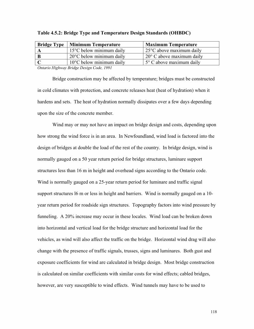
118

Table 4.5.2: Bridge Type and Temperature Design Standards (OHBDC) Bridge Type Minimum Temperature Maximum Temperature A 15°C below minimum daily 25°C above maximum daily B 20°C below minimum daily 20° C above maximum daily C 10°C below minimum daily 5° C above maximum daily Ontario Highway Bridge Design Code, 1991

Bridge construction may be affected by temperature; bridges must be constructed

in cold climates with protection, and concrete releases heat (heat of hydration) when it

hardens and sets. The heat of hydration normally dissipates over a few days depending

upon the size of the concrete member.

Wind may or may not have an impact on bridge design and costs, depending upon

how strong the wind force is in an area. In Newfoundland, wind load is factored into the

design of bridges at double the load of the rest of the country. In bridge design, wind is

normally gauged on a 50 year return period for bridge structures, luminare support

structures less than 16 m in height and overhead signs according to the Ontario code.

Wind is normally gauged on a 25-year return period for luminare and traffic signal

support structures l6 m or less in height and barriers. Wind is normally gauged on a 10-

year return period for roadside sign structures. Topography factors into wind pressure by

funneling. A 20% increase may occur in these locales. Wind load can be broken down

into horizontal and vertical load for the bridge structure and horizontal load for the

vehicles, as wind will also affect the traffic on the bridge. Horizontal wind drag will also

change with the presence of traffic signals, trusses, signs and luminares. Both gust and

exposure coefficients for wind are calculated in bridge design. Most bridge construction

is calculated on similar coefficients with similar costs for wind effects; cabled bridges,

however, are very susceptible to wind effects. Wind tunnels may have to be used to

119

simulate conditions for bridge design where wind load may be severe. Wind effects on

bridges are more critical for larger span bridges, as there is more exposed surface area.

The lateral load for a wind speed of 100 km/hr is 0.0024 MPa. Doubling the wind load

on a large, cabled bridge may increase the cost of the bridge by 5-10% depending upon

what other loads must be taken into consideration. Wind is also a factor on the “live

load”; consequently high traffic bridges are affected more than low traffic bridges.

Increases in traffic will pose a problem if wind speeds also increase and the bridge may

have to be reinforced. The wind loads on different bridge components are given in Table

4.5.3.

Table 4.5.3: Differences in Wind Effects on Bridge Components Structural Component Windward Load

(pounds/square foot) Leeward Load (pounds/square foot)

Trusses, columns, arches 50 psf 25 psf Beams 50 psf - Large flat surfaces (decks) 40 psf - (Ontario Highway Bridge Design Code, 1991)

Climate will have an effect on the cost of bridge construction in terms of the

strength of bridge piers, should the temperatures fall and more ice form. According to

Christopher R. Adams, (http://www.esig.ucar.edu/socasp/weather1/adams.html), ice

jams threaten bridges and can close major highways. There are two types of impact from

ice, ice accretion on the superstructure and ice pressure on substructure. Ice accretion,

which is expressed as the unit weight of ice, can exert a force of 9.8 KN/cubic metres on

a structure. Ice accretion is a function of temperature plus precipitation plus wind speed.

The bridge structure itself seldom sustains an impact from ice accretion as it is already

designed for much greater forces. Other structures on the bridge, such as the luminaries,

must be designed for ice accretion. There will be a cost imposed if these structures must

120

be upgraded. There are currently four ice zones in Canada; most of the ice accretion

problems are in the eastern part of the country (Ontario Highway Bridge Design Code,

1991).

Ice pressure is also a consideration in bridge construction and may add to the

costs. While scour is the leading cause of bridge failure, there have been bridge failures

due to ice jams. The Upper Steel Arch Bridge constructed over the Niagara River,

between the United States and Canada, failed in 1938 and was washed downriver after an

ice jam caused structural damage to the bridge abutments and hinge supports of the arch

Bridges over Niagara, http://www.iaw.com/~falls/bridges.html). When bridge piers are

situated in water, they must be sufficiently sturdy to sustain the effects of ice, if ice

normally forms in the area. Ice thickens rapidly in the cold and is insulated by snow. Ice

is weaker than steel or concrete but can still do damage. Damage to bridge piers may be

caused by moving sheets (ice floes), static ice or ice jams. Static ice creates pressure by

expansion during freezing. Ice jams result in the spring when unequal thawing occurs.

The size of the bridge piers is directly related to the ice strength and thickness. Ice force

and strength is determined by its thickness and the pattern of breakup. Climate change

that produces more or less ice will have an impact on the cost of bridge design. The ice

loads imposed by different types of moving ice are given in Table 4.5.4.

Table 4.5.4 Ice Loads Imposed by Moving Ice Ice Type Ice Breakup Ice Pressure Disintegrated At melting temperatures 400 kPa Intact At melting temperatures 700 kPa Large Sheets Internal movement of sheet 1100 kPa All Below melting temperatures 1500 kPa Ontario Highway Bridge Design Code, 1991

121

Ice loads are different for different types of bridges but are only usually

applicable to piers of substantial mass and dimensions. Ice problems can be expected for

solid shaft piers greater than one metre in thickness where the top of the footing to the

centre of ice action is less than three times the shaft thickness. Slender and flexible piers

are not suitable. The Confederation Bridge over the Northumberland Strait, between the

mainland and Prince Edward Island, is a good example of a bridge that would have to

sustain ice impact. Special ice shields are part of the design of this bridge and have

added to the cost of construction. Ice, in the form of permafrost in soil, also may have a

stabilizing effect on the substructure of both roads and bridges. When climate changes,

bridges may be destabilized by the loss of strength in the supporting soil if the

temperature increases.

Water, in the form of precipitation and humidity changes due to climate change,

may have some minor effects on the capital costs of bridges. High humidity and fog will

facilitate concrete breakdown, especially when coupled with increased concentrations of

oxides of sulphur, nitrogen or carbon in the air (acidity). The high humidity and fog

coupled with the acidic compounds in the air will also facilitate the corrosion of steel..

Wet-dry cycles will facilitate concrete breakdown and the corrosion of steel, especially

where acidic compounds may be present. Keeping concrete dry is critical to preserving

it. (Theodor, N.C. and Al-Bazi, G. MTO, 1997). Carbon dioxide will diffuse into concrete

and react in the presence of water, causing the concrete to become less alkaline. If its pH

drops below 9-10, the passivity of concrete breaks down and general corrosion can occur.

4.5.1.3: Ditches and Drains

Ditches and drains are associated with the storm water management system for

the highway. Ditches and drains are necessary to carry off water that does not infiltrate

122

hard surfaces, such as roads and rooftops. Roads and roofs are usually sloped to carry off

rainfall. Drainage systems are usually put in place with road construction. An

improper/inappropriate drainage system installation may result in washouts and road

destruction and flooding (Ontario Ministry of Transportation

http://www.mto.gov.on.ca/english/engineering/drainage/section9.htm). Ditches and

drains are designed to carry off water that normally flows through an area plus the storm

water that results from single events. The components of storm water management

include stream channels, storm sewers, roadside ditches, drains, catchment basins and

detention facilities. The storm water management system must be considered in

conjunction with culverts and bridges, dams and dikes. The hydrologic/hydraulic

analysis to determine the design of receiving drainage systems should include

calculations of peak flows, water surface elevations and flow velocities at different

reference points and for different frequencies for the area that is to be drained.

Roadways must be designed with adequate drainage systems or rainwater will

collect and form puddles or undercut the subsurface of the road. There must be sufficient

size in culverts that storm water will not erode the embankments around the drain and

cause failure of a roadway above it. The design of the storm water management system

must include consideration for flow rates, channel erosion, roadway surface flooding, the

potential for scour, identification of catchment inputs, selection of precipitation data,

culvert analysis, bridge analysis, flow in open channels, flow in storm sewers, flow in the

storm water management system and detention facilities. Bank stabilization and grading

are also an important component of drainage management. Drainage systems for

roadways may also be part of larger water management systems, particularly in flood-

123

prone areas where all of the components of the drainage system must be able to handle

large volumes of water in the event of a flood.

Climate directly affects the capital costs of ditches and drains in terms of the size

of culverts that are installed; culvert sizes are determined by return periods for extreme

events and by the amount of runoff that is normally expected. Larger ditches, drains and

culverts increase the cost of the roadway. The calculations that may be used to design

storm events and dictate the design of a storm water management system require the type

and duration of precipitation, the rainfall records and station and the input parameters.

The parameters to be calculated include peak flows, water surface elevations, flow

velocities and runoff volumes. The calculations related to precipitation may include

specifications for frequencies of precipitation events (low flow, 2 year events, 5 year

events, 10 year events, 25 year events, 50 year events, 100 year events, regulatory storm

levels). The highway drainage systems must be designed such that the flow of water

along the highway is kept within reasonable limits during major storms. In Ontario, the

guidelines state that the crown of the freeway should not become submerged, the depth of

flow at the crown of an arterial road should not exceed 0.15 metres and the depth of flow

at the gutter should not exceed 0.4 metres.

The calculations that determine flow rates translate into culvert sizes, ditch depths

and detention facility capacity changes if there is a change in precipitation. Increased

precipitation, increased extreme precipitation events and the increase in runoff that

accompanies this increased precipitation will result in the need for larger culverts, deeper

ditches and larger storm water detention facilities. Road slopes may have to be increased

in order to carry off increased amounts of water more rapidly. Decreased precipitation, a

124

decrease in extreme precipitation events and less runoff will result in overcapacity in

existing storm water management facilities. Full storm water management computation

requires culvert analysis, bridge analysis, flow in open channels, assessment of channel

erosion (including roadside ditches), flow in storm sewers, roadway surface flooding,

flow in storm water management detention facilities and scour potential to be calculated.

In developing a storm water management system, the before and after

development peak flow depths and velocities must be calculated for design flow

frequency and regulatory storm flow (e.g. 1 in 100 year event). The post-development

peak flow rate must be less than the design flow capacity. The freeboard requirements

(for the highway roadside ditches only) are satisfied if the post-development depth of

flow is less than the allowable depth of flow and the post-development flow velocity does

not cause erosion or scour. The post-development headwater levels, storage volumes and

emergency spillway depths are all subject to similar criteria. Detention facilities are

usually designed to specifications in terms of surface area and depth. There are specific

configurations for inlet and outlets, flow splitters and emergency spillway locations,

types and capacities. Emergency spillways should be designed to pass the regulatory

flood without failure, under blocked outlet conditions. A change in the type, amount

and/or distribution of precipitation for an area may result in a complete change in all of

the specifications for a given area.

Climate factors into the costs of construction of ditches and drains, and provision

may have to be made for water management during the construction phase. Construction

timing, construction phasing, stabilization requirements, siltation fencing locations,

access/mud mat locations, catch-basin controls, rock check dam locations, siltation

125

basins, topsoil stockpile storage locations, inspection and maintenance may have to be

altered depending upon the rainfall and flows during construction.

4.5.2: Operating Costs

Operating costs are those costs associated with maintaining the use of the road,

bridge or storm water management system. Operating costs may also involve activities

such as collecting tolls for roads and bridges and the raising and lowering of lift bridges.

These costs are not likely to be affected by changes in climate. Operating costs that will

be affected by climate change can be broken down into the maintenance costs associated

with roads, bridges, storm water management systems and winter control costs. Winter

control costs, where they exist, are often reported separately from other road system

costs. Winter control is often a very high proportion of the operating costs for a roadway;

it is often in the best interests of good fiscal management to track these expenditures

separately. Operating costs may be reported as capital costs when the magnitude of the

cost of repairs becomes large. Often, at this point, a decision must be made whether to

repair or replace. An analysis of the expected lifespan of the structure, whether it is a

road, bridge or drainage system component may be made in order to determine if repairs

will extend the life of the structure enough to justify the expenditure. If repair is no

longer cost-effective, replacement will be undertaken.

4.5.2.1: Roads

The operating costs for roads are predominantly maintenance costs although there

may be features such as tollbooths that are not directly involved in road maintenance and

are included in the operating costs for the road. Maintenance of the roadway for asphalt

and concrete roads usually involves hardtop or concrete patch and washout repair,

cleaning, flushing and sweeping, sign repair or replacement, marking and painting. For

126

gravel roads, the road must be patched, washouts repaired and resurfaced. Chemicals for

dust control, such as calcium chloride, are often applied. Shoulders on roads, signs, curbs

and sidewalks must be repaired or replaced. Often replacement of curbs is done at the

same time as road replacement or resurfacing. Vegetation control is also part of road

maintenance. Vegetation control involves tree-trimming, brush clearing, mowing and

spraying.

Operating costs for roads include maintenance costs for structures and features

that allow safe use of the roadway and that will prolong its lifespan. When maintenance

costs are reduced, safety may be compromised and the longevity of the roadway may be

reduced, resulting in the need for greater capital expenditures. The environment and

human activities will cause deterioration of a road over time; expenditures on operations

reduce the need for costly replacements later. There is a point in time where a roadway

must be replaced; it is no longer cost-effective to continue to repair it. Often this point is

coincident with the need to upgrade the road for increased traffic or to accommodate new

materials or new structural elements in the design. Roads may be patched over top of

patches but the road surface becomes progressively bumpier and traffic flow will

eventually be impeded.

New materials that are being utilized in road construction may alleviate some of

the need for road repair. Much of the repair of roads is related to the formation of

potholes. The formation of potholes is related to the capacity of the road surface to

withstand the expansion and contraction of the road surface itself and water that may seep

into the pavement. The incorporation of materials such as crushed rubber tires improves

the ability of the road to withstand expansion and contraction. The need for road repair

127

may diminish in the future and operating costs may subsequently drop with these

improvements.

4.5.2.2: Bridges

Bridge maintenance activities involve repairs to the bridge deck, repairs to

culverts, repairs to guard rails, repairs to support structures (structural steel costs $1.50-

$2.00 per lb $US 1995), washing, which is often done with road cleaning, repairs to wing

walls and bank stabilization (especially bridges over water), repairs to the lift

mechanisms if present and repairs to bridge drainage systems. Bridge maintenance may

also involve sealing. Keeping water out is the key to the durability of concrete and steel

in bridges. Concrete and steel are subject to attack by salts and sulphates. Concrete and

steel are subject to attack by sulphates from rain (acid rain) and groundwater. This may

necessitate the replacement of one type of cement with a sulphate-resistant type. Freeze-

thaw cycles are very hard on concrete and dense, well-compacted cement must often be

used where freeze-thaw cycles are a problem. Alkali-silica reactions are an internal

reaction in the concrete that causes swelling and cracking. High alumina cement

conversion in conjunction with high humidity will very rarely cause a reaction. Salt

crystallization in concrete will result from the movement of salts by capillary action and

rise of salt-bearing water. De-icing salts causes salt scaling on horizontal slabs.

Bridge maintenance is intended to minimize effects of traffic load, environmental

strain and de-icing chemicals. The environmental strain on bridges results in

deterioration due to a number of factors. These factors include creep, shrinkage,

humidity, moisture, swelling and variation in vehicular load such that expansion devices

may not behave properly. Climate affects bridge maintenance in terms of the amount and

the type of maintenance. Climate can also affect the amount of maintenance on bank

128

stabilization structures. Wetter soils will slump. Banks may destabilize from water–

freeze thaw, wave action, slumping from heavy rains and wave action. Waves and salt

water will affect support structures. Freeze-thaw, wet-dry, salt, high temperatures and

low temperatures will affect surface concrete and cause it to spall and crack which will

cause rebar to be susceptible to corrosion. Exposed rebar corrodes more easily and the

bridge will lose its strength and structure if the rebar is damaged. Damaged rebar leads to

bridge deterioration and replacement. Bridge drainage systems may also be clogged by

debris, causing poor drainage on the deck. The bridge substructure may be damaged by

ice, both static and moving, and may need to be repaired.

Bridge decks, especially the expansion joints, are particularly susceptible to

corrosion from de-icing salts that are applied to the roadway on the bridge. The

substructure is less susceptible to the effects of de-icing chemicals. The roadway on a

bridge often “ices up” sooner and more than the road itself. More de-icing salts may be

applied to bridges as a consequence. Salt has the greatest effects on the metal

components of a bridge. The metal components of a bridge include the expansion joints;

lift mechanisms, bridge drainage systems and guardrails. Salt can also cause or enhance

concrete spalling. Concrete spalling results in the ultimate deterioration of the concrete

and a loss of strength in the structure. Concrete spalling also exposes the reinforcing

materials in the concrete. The reinforcing materials, or rebar, are susceptible to corrosion

unless non-metallic, galvanized or stainless steel materials are utilized. The new

standards for bridge design for Canada (CHBDC) will utilize corrosion-resistant

materials in the construction of new bridges. Other de-icing chemicals are available such

as acetate compounds that do not corrode metal to the same degree as the chlorides

129

(salts). Bridges that are constructed largely of steel, such as the large suspension bridges

forming the Thousand Islands Bridge from Gananoque, Ontario to New York, utilize

acetates instead of chloride salts. The cost, however, is much higher. Sodium

magnesium calcium acetate costs approximately $2000 Canadian per metric tonne,

whereas sodium chloride (road salt) costs $65 Canadian per metric tonne.

Bridges may be constructed from aluminium and iron, concrete, steel, stone or

wood. Aluminium and iron are denser than concrete, which is denser than stone or wood.

Both concrete and steel are subject to corrosion; concrete will spall and the steel

reinforcing mesh within the concrete will corrode if exposed. Wood tends to decay.

Many of the wooden bridges in the country have been replaced with concrete and steel

structures as they became unusable. Covered wooden bridges still exist in eastern parts

of Canada, through Quebec and the Maritimes. The primary purpose of a covered bridge

was to shed snow and stop the decay of the bridge deck but covered bridges are usually

kept as historic sites and tourist attractions. Most highway and railway bridges in service

in Canada are composed of concrete and/or steel. Railway bridges were often metal truss

bridges as these bridges were designed for more weight. Railway bridges do not usually

require de-icing salt to maintain their safe utilization by trains; the weight of the train is

usually sufficient to clear any ice. Railway bridges are not subject to the same

deterioration from de-icing salts as steel highway bridges. Highway bridges may be

waterproofed to reduce maintenance costs and compounds such as urea and the acetate

compounds may be used to reduce corrosion.

Maintenance practices on bridges must deal with corrosion and fretting fatigue.

Fretting fatigue is caused by two metal surfaces continuously subjected to small repetitive

130

sliding motions. An increase in contact pressure results in a decrease in the fretting life if

pressure is high enough to prevent sliding movements. A corrosive environment

decreases fretting life. Bearings and expansion joints are subject to both fretting fatigue

and road salt corrosion. High hardness, higher strength steels are more susceptible to

fretting fatigue than lower strength structural steels. Corrosion problems with bridges

began with the introduction of salt in the 1960s and the damage from de-icing salts began

to show up in the 1970s. There are more problems with deterioration in modern bridges

than older bridges because modern bridges are longer and have more expansion joints.

Deterioration in bridges may occur as a result of the daily cycles of expansion during the

day and contraction at night. Concrete and steel bridges also expand in the summer and

contract in the winter. In order to minimize these effects, bridge maintenance is often

performed annually. Bridge preventative maintenance involves cleaning all exposed

surfaces, drains, bearings and seats. Minor repairs are also done as part of preventative

maintenance. Bridge inspection is also often performed periodically to determine the

overall condition of the bridge. There are a number of factors that determine the amount

of bridge maintenance. The total bridge deck area is a major determinant of bridge

operation and maintenance costs, as is the age of the bridge stock on average. Climate

factors that may influence the maintenance costs include the average number of freeze-

thaw cycles per year (number of days during which the minimum and maximum

temperature recorded are above and below the freezing point. The amount of de-icing

road salt that is applied per year is also a factor. The traffic intensity, which can be

described as the total amount of vehicle-km/ street area, is also a factor. Another factor

131

in bridge maintenance costs is the presence of bridges whose construction predates

improved concrete composition.

4.5.2.3: Ditches and Drains

Operations costs for ditches and drains include such activities as the cleaning and

clearing of the drainage system, repairs to culverts and digging of ditches. The drainage

system must remain clear and operate at its design capacity in order to be useful and

serve its function properly. The storm water management system is a means of extending

the lifespan of the road and keeping it safe. Culverts and drains may become clogged and

not function if debris accumulates. Storm water detention areas may accumulate silt and

will not function at capacity. Ditch and drain maintenance also involves vegetation

control. Vegetation can overgrow and interfere with the functioning of the drainage

system. Grass mowing and brush control in some types of ditches is important to

maintain flow. Vegetation control also prevents the trapping and accumulation of debris.

Vegetation growth is affected by climate. Increases and decreases in temperature and

precipitation will affect vegetation growth and the amount of mowing that must be done.

Heavy rainfalls wash debris, including soil materials and tree limbs, into the storm water

management system. Complete clogging of the system will occur if these materials are

not periodically removed. The silt that is washed into the storm water management

system through erosion caused by heavy rainfall will also accumulate in storm water

detention areas and may have to be periodically removed.

4.5.2.4: Winter Control

Winter control includes such activities as road patrol, sanding, salting, plowing

and snow removal, culvert thawing and the installation of snow fencing. The amount and

type of winter control varies by municipality. Some municipalities, such as the City of

132

Vaughn, offer clearing of sidewalks and windrows as part of their snow removal services.

This extra service will substantially inflate winter control costs. Some municipalities do

not provide as much side street clearing as other municipalities and their winter control

costs are therefore much lower than their climate would normally reflect. Winter control

is particularly affected by changes in temperature and precipitation resulting in more or

less snow and ice. Wind may be a confounding factor in winter control. Some of the

costs of winter control may be exacerbated by the design of roadways. More frequent

snowfalls may increase the costs of snow clearing, sanding and salting if the snowfalls

are sufficiently heavy. Greater amounts of falling snow or an accumulation of snow with

no thawing in between snowfalls may necessitate the removal and stockpiling of snow,

which is very expensive.

Wind causes snow to blow, decreasing visibility for snowplow operators and

accumulating in drifts. Blowing snow can therefore increase removal costs. Fluffy snow

begins to move when the wind speed approaches 20 km/hr and hard snow may resist

movement up to 85 km/hr wind speeds. Snow usually ceases to blow when the wind

speed falls below 24 km/hr. Most snow transport is within one metre of the road surface.

If the blowing and drifting of snow is severe on highways, it may be necessary to install

snow fencing and incur the additional costs associated with this activity (Tabler, R.

1994).

Greater evaporation may also result from blowing snow than stable snow,

resulting in less accumulation of snow over the winter and less need for costly snow

removal. Plowing costs may increase, but removal costs may decrease. Blowing snow

may also complicate snow removal, however, and necessitate more frequent snow

133

removal as snow blows back into plowed areas. Blowing snow also slows snow removal

operations as visibility becomes poor and plows must reduce their speed. Higher relative

humidity results in less snow evaporation and more accumulated snow. Areas with high

relative humidity are also often subject to snowstorms. This phenomenon is known as a

“lake effect” and causes snowstorms in the Buffalo, US area. Climate change in the areas

that are particularly subject to lake effects may result in much higher changes in winter

control costs than climate change in areas that are not subject to these effects.

Lower temperatures result in less snow evaporation; the evaporation rate for snow

doubles with every 10°C rise in temperature (Tabler,R.., 1994). Lower temperatures also

affect culvert thawing, as culverts become more prone to freezing. If culverts are not

thawed, drainage may be blocked and water will accumulate. Lower temperatures will

result in more ice formation on roadways and increase the amount of sand and/or salt that

must be applied to maintain safety levels on the road. Lower temperatures, in

conjunction with precipitation, will increase winter control costs; higher temperatures

when precipitation occurs will have the reverse effect on winter control costs.

4.5.3: Summary

Capital costs and operating costs for roads, bridges and storm water management

systems are affected by climate in a number of ways. Depending upon the manner in

which climate changes, costs may be increased or decreased. The primary effects of

climate on capital costs and operating costs for these structures are as follows:

4.5.3.1: Roads Capital Costs

The major climate-related capital costs for roads include:

• Decrease (increase) in permafrost that decreases (increases) the cost of road

building

134

• Decrease (increase) in rate of permafrost thawing that decreases (increases) the

frequency of road replacement

• Increase in temperatures that decrease the winter/ice road season, necessitating

construction of all weather roads

• Decrease (increase) in temperatures that requires an increase (decrease) in the

depth of the roadbed and more (less) fill to protect against frost heave

• Less (more) precipitation that causes an increase (decrease) in the stability of the

roadbed, requiring less (more) depth of underlay

• Decrease (increase) in frequency of avalanche conditions necessitating the

construction of fewer (more) snow sheds and tunnels

4.5.3.2: Roads Operating Costs

The major climate-related operating costs for roads include:

• Less (more) snow that decreases (increases) the cost of snow plowing, sanding

and salting

• Less (more) frequent heavy snowfalls that decrease (increase) the cost of snow

removal

• Fewer (more) freeze-thaw cycles that decrease (increase) the number of potholes

• Shorter (longer) periods of cold temperatures that decrease (increase) the amount

of frost heave in the roadbed, creating less surface cracking

4.5.3.3: Bridges Capital Costs

The major climate-related capital costs for bridges include:

• Decreased (increased) temperatures that result in ice cap formation (reduction)

and produce lower (higher) water levels that require lower (higher) bridges

135

• Decreased (increased) temperatures that result in more (less) ice formation and

require larger (smaller) bridge piers to guard against sea and lake ice damage

• Decreased (increased) precipitation that results in less (more) runoff and scour

and requires smaller (larger) substructure

• Increased wind velocity that results in the need for stronger super and substructure

• Decreased wind velocity that results in the need for less strength in the

substructure

• Increases in temperatures (above 0°C) with precipitation that result in less use of

de-icing salts and longer bridge life span with less frequent bridge replacement

• Increases in temperature (above -10°C) with precipitation that result in greater use

of de-icing salts and shorter bridge life span with more frequent bridge

replacement

• Decreases in temperatures (below 0°C) with precipitation that result in greater use

of de-icing salts and a shorter bridge life span with more frequent bridge

replacement

• Decreases in temperatures (below -10°C) with precipitation that result in less use

of de-icing salts and a longer bridge life span with less frequent bridge

replacement

4.5.3.4: Bridges Operating Costs

The major climate-related operating costs for bridges include:

• Increases in temperatures (above 0°C) with precipitation that result in less use of

de-icing salts and less bridge repair

136

• Increases in temperature (above -10°C) with precipitation that result in greater use

of de-icing salts and more bridge repair

• Decreases in temperatures (below 0°C) with precipitation that result in greater use

of de-icing salts and more bridge repair

• Decreases in temperatures (below -10°C) with precipitation that result in less use

of de-icing salts and less bridge repair

• Increases in seasonal temperature range that increase concrete spalling and result

in more patching

• Decreases in seasonal temperature range that decrease concrete spalling and result

in less patching

4.5.3.5: Storm Water Management System Capital Costs

The major climate-related capital costs for storm water management systems

include:

• Less (more) frequent heavy precipitation events resulting in decreased (increased)

costs for smaller (larger) culverts, shallower (deeper) drains, smaller (larger)

storm water detention facilities, decreased (increased) grading of side slopes to

increase (decrease) the slope on ditches

4.5.3.6: Storm Water Management Operating Costs

The major climate-related operating costs for storm water management systems

include:

• Lighter (heavier) overall precipitation resulting in decreased (increased) costs of

drain cleaning, ditch clearing and storm water detention facility dredging

137

• Less (more) frequent heavy precipitation events that cause flooding and washouts

of culverts and necessitate replacement or repair of various components of the

storm water management system

4.6: The Costs of Adaptation

The costs of adaptation to climate change may be broken into capital costs and

operating costs for roads, bridges and storm water management systems.

4.6.1: Capital Costs

Capital costs associated with climate change adaptation include the additional

costs imposed on road reconstruction and new construction, bridge reconstruction and

new construction and storm water management reconstruction and new construction.

While reconstruction may be included in operating costs for many levels of government,

large reconstruction costs are usually included in capital expenditures. There are many

options open to governments in the maintenance of a road system in terms of the amount

of repair that is performed on a road, bridge or storm water management system. Roads

may be patched indefinitely but the road becomes progressively more difficult to travel

on and speeds must be reduced. Bridges may be patched almost indefinitely but the costs

of repair often must be assessed with respect to the ability of the bridge to sustain the

“live load” or traffic. Drainage systems may be temporarily repaired year after year but

there is a cost to the road system in so doing. There is less flexibility in the

reconstruction versus repair of these storm water management systems as these systems

are often the weak points in maintaining the highway system. A poorly maintained

drainage system will result in much higher costs for its associated road system.

4.6.1.1: Roads

The impact of climate change on the capital cost of roads can be broken into

138

general effects on all roads plus a few special, high-impact cases. All roads will sustain

some impact of changes in temperature, particularly changes in freeze-thaw cycles,

changes in the depth of frost (frost heave) and the potential destruction of the road system

due to culvert washouts. Temporary roads in the north, also known as “ice roads” or

“winter roads” will sustain a particularly high impact from warming. These roads will

not be useable if the temperature warms substantially. These roads may have to be

replaced with more permanent structures at a very high cost. Roads on permafrost will

also be very susceptible to changes in temperature. The loss of permafrost destabilizes

the roadbed and results in the need for major road reconstruction, often over very large

areas. Road building costs are higher for the roads on permafrost in the Northwest

Territories. Roads on permafrost cost approximately $500,000 per km to build; roads on

non-permafrost cost approximately $350,000 per km to build. Roads on permafrost are

constructed differently and must be constantly monitored for the loss of the integrity of

the roadbed (Larry Purcka, Northwest Territories Transportation, personal

communication). The loss of permafrost means that new road construction will be less

expensive throughout the discontinuous permafrost zone but the existing road system will

sustain heavy impact as the permafrost slowly disappears from the roadbed.

4.6.1.1.1: All Roads

The capital costs for roads will be affected by the need for greater expenditure

when a road is built. Capital expenditures for roads will sustain climate change impact

from the need for greater amounts of fill to produce a more stable roadbed where the frost

line may extend further into the soil profile. Capital expenditures for roads will also

sustain more climate change impact where the stability of the roadbed may be affected by

increases and decreases in the amount of precipitation and changes in the depth of frost.

139

Ice lenses tend to form at the frost line and the roadbed must be sufficiently well drained

that moisture does not collect at the normal, expected frost depth. Excess moisture at the

frost line will freeze and expand. Ice lenses also draw moisture from the surrounding

soil. A concentration gradient is set up through the soil profile as water is withdrawn

from the soil matrix, resulting in the movement of water within the soil profile toward the

developing ice lens. The resulting ice lenses are large and cause heaving of the road

surface in the winter while they are forming and slumping in the spring when they melt

and dissipate. The road surface cracks and is eroded by the passing traffic when this

happens. Many parts of the country restrict individual truck weights on the road network

in the spring to prevent or minimize the damage that frost heave causes. Much of the

heavier weight truck traffic moves over the road system through the winter when the sub

grade is frozen and able to withstand heavier loads.

4.6.1.1.2: Winter/Ice Roads

Ice/winter roads are temporary roads that are functional in the winter only. They

are created from a mixture of soil, snow and/or ice and may be created on the frozen

surface of lakes and rivers. Winter roads may be roads that are not passable in the

warmer weather due to high moisture content in the soils. Winter roads often involve ice

crossings over rivers and lakes. The government of the Northwest Territories often

utilizes temporary bridges on its major winter roads to ensure safe passage of vehicles

(Larry Purcka, Northwest Territories government, personal communication).

The Ontario government recently spent $2.7 million (1999) for the construction

and maintenance of over 2700 km of ice/winter roads linking the northern part of the

province. In the Northwest Territories, all weather roads service only a portion of the

communities. Most communities are linked, one way or another, by ice/winter roads.

140

The town of Fort Chipewyan, which is land-locked at the northern boundary of Alberta,

is only accessible from the south by a temporary winter road running north from Fort

McMurray. All freight must otherwise move by air. Most heavy equipment, construction

materials, fuel and heavy goods move into the remote communities during the winter

over this system of roads. It is estimated that approximately 10-15% of the total annual

flow of goods in the Mackenzie Valley (Northwest Territories / Yukon) moves over

winter roads (EPA, 1998). Table 4.6.1 shows a summary of the quantity and distribution

of winter/ice roads in Canada.

Table 4.6.1: Summary of Quantity and Distribution of Winter/Ice Roads in Canada Province Winter/Ice Roads (publicly maintained) 1 Total Km

(approximate) Alberta 0 provincial but two major roads maintained by municipality of

Wood Buffalo through Fort Chipewyan (285 km) and to the Saskatchewan border (100 km), one road federally maintained from Fort Chipewyan to Fort Smith (228 km) 2

650

British Columbia

0 3

Manitoba 1000 km provincial, 600 km municipal 4 1,600 New Brunswick 0 Newfoundland 0 5 Nova Scotia 0 Ontario 2700 km provincial and municipal (8 km maintained by

Moosonee) 6 2,700

Prince Edward Island

0

Quebec ~3000 (1305 provincial)7 3,000 Saskatchewan ~500 (381 km maintained by province - four major ice roads –

Athabasca (180 km), Stoney Rapids-Fond du Lac (160 km), Wollaston Lake crossing (36 km) and Riverhurst crossing (5 km))8

500

Northwest Territories

1400 km provincially maintained 9 1,400

Nunavut 0 10 Yukon 0 provincial, very few municipal (1 km ice bridge maintained by

the municipality of Dawson City) 11 10

Total Km 9,860 1 There are also additional winter roads that have been constructed and maintained by the private sector which are publicly funded; there is also a large number of private winter roads developed and maintained by the mining and forest industries

141

2 Bill Kenny, Alberta Infrastructure, personal communication; Municipality of Wood Buffalo; Wood Buffalo Park

3 Dave Moore, British Columbia Ministry of Transportation and Highways, personal communication 4 “Ice Road Blitz”, Transport Canada publication ISSN0710-0914 TP 2711 E 5 Gerry Goss, Newfoundland Works, Services and Transportation, personal communication 6 “Bear Country”, in-flight magazine of Bearskin airlines; Town of Moosonee 7 estimate based on Ontario figures, provincial figure derived from http://www.mtq.gouv.qc.ca/regions (routes d’access aux resources) 8 estimate based on Manitoba figures, provincial figure from http://www.highways.gov.sk.ca/travellers_information/ice_roads.htm; Saskatchewan Highways and Transportation, Prince Albert office 9 Larry Purcka, Northwest Territories Transportation, personal communication 10 Doug Sitlin, Nunavut Community and Transportation, personal communication 11 Bernie Cross, Yukon Community and Transportation Services, personal communication

The yearly costs for building and maintaining ice roads are quite variable,

normally ranging from $2,000 to $5,000 per km (Gary McClelland, Saskatchewan

Highways and Transportation; Bear Country; Jennifer Tallman, Abitibi Consolidated

Iroquois Falls). Maintenance costs for the two main provincial ice roads for

Saskatchewan average only slightly less than the initial opening costs (Table 4.6.2). The

province of Saskatchewan is currently building a 180 km winter road from Points North

Landing to Black Lake at a cost of $8 million to supply the communities in the Lake

Athabasca area (Saskatchewan Highways and Transportation

http://www.inac.gc.ca/nr/prs/s-d1997/1-9730.html) resulting in an initial cost of $44,000

per km. This would be expected to drop in subsequent years. The costs for winter/ice

roads are summarized in Table 4.6.2.

Table 4.6.2: Opening and Maintenance Costs for Winter/Ice Roads Road Initial Opening Maintenance Distance

(km) Normal Duration for Use

Hwy 905 Stony Rapids to Fond du Lac

$55,000 ($1,719/km/yr)

$40,000 ($1250/km/yr)

32 8-12 weeks (8 clearings)

Hwy 905 Wollaston Lake Landing to Wollaston Lake settlement

$73,000 ($1,431/km/yr)

$50,000 ($980/km/yr)

51 8-12 weeks (10 clearings)

142

All weather roads are considerably more expensive to build and maintain. In

northern Ontario, construction of an all-weather road will cost at least $85,000 per km

plus bridges. An average bridge for an all weather road in Ontario will cost between

$65,000 and $150,000 per bridge (Jennifer Tallman, Abitibi Consolidated Iroquois

Falls). An all-weather replacement for the winter road at Grandmother’s Bay in northern

Saskatchewan cost the Saskatchewan provincial government $1.45 million dollars for

11.7 km of road ($124,000 per km) in 1997 (Saskatchewan Executive Council

(http://www.gov.sk.ca/newsrel/1995/04/11-167.html). Construction of an all weather road

where no road previously existed is more expensive than replacement of an existing road.

The “Route du Nord”, a gravel all weather road from Chibougamou to Nemiscau in

Quebec, cost the Quebec provincial government approximately $350,000 per km in 1999

to build. (http://www.gov.sk.ca/newsrel/1995/04/11-167.html).

All weather roads require maintenance in addition to the capital expenditure. At

present, British Columbia spends approximately $4,000 per lane-km in road maintenance

(BC Ministry of Transportation and Highways Annual Report 1999-2000, pg17). All

weather gravel roads must be graded, potholes patched and culverts replaced. The

replacement of an ice/winter road with an all weather road does not mean that the cost of

ice/winter road construction and maintenance will be completely forgone. Large capital

expenditures and the continuation of maintenance costs will accompany the construction

of all weather roads to replace the ice/winter roads. The replacement of an ice/winter

road with an all weather road will not necessarily follow the same route. According to

Parks Canada staff in Wood Buffalo Park, the ice road between Fort McMurray and Fort

143

Chipewyan will likely follow another route. This is often done to minimize bridge

construction and its associated high costs.

Climate change will affect the winter/ice roads in two ways. The season may be

shortened such that these roads are no longer a viable means of transportation for the

affected communities in the north. S.C. Lonergan, et al (1993) identified shortening of

the ice road season as a major climate change impact for the north. The permafrost

underlying these roads (and many all weather roads) in the northerly parts of Canada is

receding. Every year more of the permafrost disappears in some areas. Winter roads in

all permafrost zones (no permafrost, discontinuous permafrost and continuous

permafrost) would be affected by anything that causes a temperature rise and shortens the

length of the ice road season. All roads may be affected by permafrost changes.

The current ice road season lasts for approximately 90 days in northern Ontario

(Ministry of Northern Development and Mines, 1999) and approximately 70 days for the

300 km Ekati mine road northeast of Yellowknife in the Northwest Territories (Transwest

Mining Systems Inc.1998). In Saskatchewan, the ice roads are open 8-12 weeks of the

year (56-84 days) (Gary McClennan, Saskatchewan Highways and Transportation,

personal communication). Conditions for ice road haulage are very specific, as

evidenced by the tables developed by Saskatchewan Highways and Transportation (see

Tables in Appendix 4.6.1). A 50% loss of ice depth will result in more than a 50%

reduction in load for both types of ice. It may no longer be possible to move either the

volume or the type of freight (such as heavy mine equipment) that currently moves over

these roads during the winter/ice road season. (Saskatchewan Highways and

Transportation, http://www.highways.gov.sk.ca/travellers_information/ice_roads.htm).

144

Publicly funded winter/ice roads exist primarily in the Northwest Territories and

northern Alberta, Saskatchewan, Manitoba, Ontario and Quebec. The Yukon has a

publicly funded ice crossing in Dawson City and other isolated ice crossings are also

found across the country. Ice roads over lakes and rivers are often utilized where ferry

service must be discontinued in the winter. There are international ice crossings between

the United States and Canada used by snowmobile enthusiasts between Drummond

Island, Michigan to St.Joseph Island (18 km) and Thessalon (29 km) in Ontario

(Woodmoor, http://www.sault.com/woodmoor/news/bridge.html). Winter/ice roads are

found in CGCM1 grid boxes 183-189, 218-226, 253-263, 270-272, 295-301, 305-309,

335-343, 371-379 and 411-412. The Greenhouse Gas Only Simulation (GG1), the mean

monthly winter temperatures (November to April) within these grid boxes, are given in

Appendix 4.6.2 for the years 1961-1990, 2010-2039, 2040-2069 and 2070-2099. A

summary of the mean winter temperatures for the years 1961-1990, 2010-2039, 2040-

2069 and 2070-2099 is given in Table 4.6.3.

Table 4.6.3: Mean Winter Temperatures 1961-1990, 2010-2039, 2040-2069, 2070-2099 GRID BOX NUMBER

PRIMARY PROVINCE/ TERRITORY

MEAN TEMP 1961-1990

MEAN TEMP 2010-2039

MEAN TEMP 2040-2069

MEAN TEMP 2070-2099

183 YK -21.33 -17.49 -14.67 -10.51184 YK -20.63 -16.57 -13.20 -8.90185 NT -21.37 -17.23 -13.98 -9.61186 NT -22.92 -19.19 -16.22 -12.14187 NT -22.29 -19.06 -15.89 -12.03188 NT -21.60 -18.72 -15.69 -11.95189 NT -21.59 -18.92 -16.07 -12.30218 YK -15.38 -12.17 -10.21 -7.02219 YK -17.61 -13.82 -11.83 -8.75220 YK -14.84 -11.42 -9.03 -6.32221 NT -14.98 -11.84 -9.32 -6.82222 NT -14.44 -11.66 -8.95 -6.59

145

223 NT -14.08 -11.70 -8.93 -6.65224 NT -14.20 -11.94 -9.12 -6.51225 NT -14.46 -11.85 -8.91 -5.71226 NT -19.50 -16.60 -13.82 -9.63253 YK -9.04 -6.46 -3.85 -0.49254 YK -7.84 -5.45 -3.15 -0.88255 YK -8.49 -6.23 -3.96 -1.86256 YK -8.91 -6.74 -4.58 -2.54257 YK/NT -8.62 -6.51 -4.46 -2.39258 NT -8.28 -6.09 -4.01 -1.98259 NT -8.19 -6.43 -4.16 -1.94260 NT -8.39 -6.61 -4.51 -2.01261 NT -8.90 -6.79 -4.59 -1.90262 NT -10.85 -8.41 -6.34 -3.25263 NT -15.35 -12.44 -9.97 -6.25270 PQ -7.62 -1.15 1.38 3.56271 PQ -16.95 -12.13 -8.80 -3.94272 PQ -5.55 -0.63 1.64 3.76295 AB -4.37 -2.44 -0.16 1.27296 AB -5.17 -3.20 -1.08 0.77297 SK -6.10 -4.14 -2.00 -0.12298 SK -8.41 -6.15 -4.09 -1.87299 SK/MB -10.42 -7.90 -5.76 -3.31300 MB -11.65 -8.89 -6.43 -3.80301 MB -15.52 -12.11 -9.28 -6.09305 PQ -6.36 -0.83 2.14 4.18306 PQ -13.72 -10.11 -6.93 -2.99307 PQ -12.02 -8.70 -5.98 -2.71308 PQ -11.03 -8.35 -5.85 -2.73309 PQ -10.93 -9.13 -6.81 -3.21335 MB -6.96 -4.57 -2.46 -0.01336MB/ON -7.63 -5.00 -2.96 -0.21337 ON -11.46 -8.07 -5.71 -1.85338 ON -11.51 -8.26 -5.87 -1.95339 ON -11.21 -8.45 -5.89 -2.25340 PQ -7.76 -5.46 -3.14 -0.58341 PQ -8.74 -6.60 -4.48 -2.18342 PQ -9.62 -7.41 -5.51 -3.30343 PQ -9.20 -6.91 -5.13 -2.97371 ON -4.48 -2.10 -0.17 2.29372 ON -5.10 -2.81 -0.92 1.69373 ON -4.99 -2.81 -0.85 1.79374 ON -4.61 -2.60 -0.61 1.93375 ON/PQ -4.28 -2.60 -0.75 1.58376 PQ -4.51 -2.96 -1.38 0.67

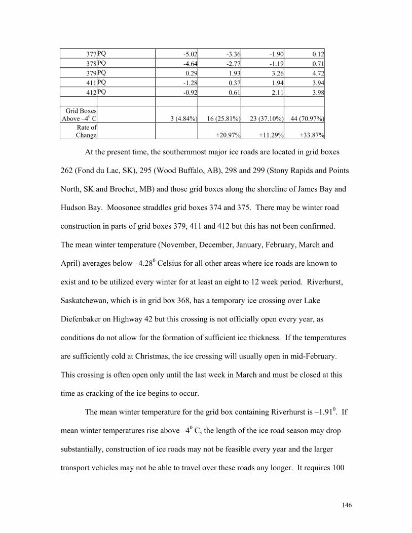
146

377 PQ -5.02 -3.36 -1.90 0.12378 PQ -4.64 -2.77 -1.19 0.71379 PQ 0.29 1.93 3.26 4.72411 PQ -1.28 0.37 1.94 3.94412 PQ -0.92 0.61 2.11 3.98

Grid Boxes

Above –40 C

3 (4.84%) 16 (25.81%) 23 (37.10%) 44 (70.97%)Rate of Change

+20.97% +11.29% +33.87%

At the present time, the southernmost major ice roads are located in grid boxes

262 (Fond du Lac, SK), 295 (Wood Buffalo, AB), 298 and 299 (Stony Rapids and Points

North, SK and Brochet, MB) and those grid boxes along the shoreline of James Bay and

Hudson Bay. Moosonee straddles grid boxes 374 and 375. There may be winter road

construction in parts of grid boxes 379, 411 and 412 but this has not been confirmed.

The mean winter temperature (November, December, January, February, March and

April) averages below –4.280 Celsius for all other areas where ice roads are known to

exist and to be utilized every winter for at least an eight to 12 week period. Riverhurst,

Saskatchewan, which is in grid box 368, has a temporary ice crossing over Lake

Diefenbaker on Highway 42 but this crossing is not officially open every year, as

conditions do not allow for the formation of sufficient ice thickness. If the temperatures

are sufficiently cold at Christmas, the ice crossing will usually open in mid-February.

This crossing is often open only until the last week in March and must be closed at this

time as cracking of the ice begins to occur.

The mean winter temperature for the grid box containing Riverhurst is –1.910. If

mean winter temperatures rise above –40 C, the length of the ice road season may drop

substantially, construction of ice roads may not be feasible every year and the larger

transport vehicles may not be able to travel over these roads any longer. It requires 100

147

cm of white ice to support a 30,000 kg vehicle. By 2099, the percentage of grid boxes

where ice roads are currently being utilized will drop by close to 70%. A breakdown of

the winter/ice road conditions in 1961-1990, 2010-2039, 2040-2069 and 2070-2099 is

given in Tables 4.6.4, 4.6.5 and 4.6.6. Table 4.6.4 contains those grid boxes where a

complete loss of winter/ice roads will likely occur. Table 4.6.5 contains those grid boxes

where the winter/ice road season may be substantially shortened and Table 4.6.6 contains

those grid boxes where the winter/ice road season is unaffected.

Table 4.6.4: Grid Boxes With Potentially Complete Loss of Winter/Ice Roads (mean winter temperatures higher than –20 C) GRID BOX NUMBER

PRIMARY PROVINCE/ TERRITORY

MEAN TEMP 1961-1990

MEAN TEMP 2010-2039

MEAN TEMP 2040-2069

MEAN TEMP 2070-2099

253 YK -9.04 -6.46 -3.85 -0.49 254 YK -7.84 -5.45 -3.15 -0.88 255 YK -8.49 -6.23 -3.96 -1.86 258 NT -8.28 -6.09 -4.01 -1.98 259 NT -8.19 -6.43 -4.16 -1.94 261 NT -8.90 -6.79 -4.59 -1.90 270 PQ -7.62 -1.15 1.38 3.56 272 PQ -5.55 -0.63 1.64 3.76 295 AB -4.37 -2.44 -0.16 1.27 296 AB -5.17 -3.20 -1.08 0.77 297 SK -6.10 -4.14 -2.00 -0.12 298 SK -8.41 -6.15 -4.09 -1.87 305 PQ -6.36 -0.83 2.14 4.18 335 MB -6.96 -4.57 -2.46 -0.01 336 MB/ON -7.63 -5.00 -2.96 -0.21 337 ON -11.46 -8.07 -5.71 -1.85 338 ON -11.51 -8.26 -5.87 -1.95 340 PQ -7.76 -5.46 -3.14 -0.58 371 ON -4.48 -2.10 -0.17 2.29 372 ON -5.10 -2.81 -0.92 1.69 373 ON -4.99 -2.81 -0.85 1.79 374 ON -4.61 -2.60 -0.61 1.93 375 ON/PQ -4.28 -2.60 -0.75 1.58 376 PQ -4.51 -2.96 -1.38 0.67 377 PQ -5.02 -3.36 -1.90 0.12

148

378 PQ -4.64 -2.77 -1.19 0.71 379 PQ 0.29 1.93 3.26 4.72 411 PQ -1.28 0.37 1.94 3.94 412 PQ -0.92 0.61 2.11 3.98

Table 4.6.5: Grid Boxes With Shortening of Winter/Ice Road Season (mean winter temperatures between –20 C and –40 C) GRID BOX NUMBER

PRIMARY PROVINCE/ TERRITORY

MEAN TEMP 1961-1990

MEAN TEMP 2010-2039

MEAN TEMP 2040-2069

MEAN TEMP 2070-2099

256 YK -8.91 -6.74 -4.58 -2.54 257 YK/NT -8.62 -6.51 -4.46 -2.39 260 NT -8.39 -6.61 -4.51 -2.01 262 NT -10.85 -8.41 -6.34 -3.25 271 PQ -16.95 -12.13 -8.80 -3.94 299 SK/MB -10.42 -7.90 -5.76 -3.31 300 MB -11.65 -8.89 -6.43 -3.80 306 PQ -13.72 -10.11 -6.93 -2.99 307 PQ -12.02 -8.70 -5.98 -2.71 308 PQ -11.03 -8.35 -5.85 -2.73 309 PQ -10.93 -9.13 -6.81 -3.21 339 ON -11.21 -8.45 -5.89 -2.25 341 PQ -8.74 -6.60 -4.48 -2.18 342 PQ -9.62 -7.41 -5.51 -3.30 343 PQ -9.20 -6.91 -5.13 -2.97

Table 4.6.6: Grid Boxes With Little/No Impact on Winter/Ice Roads (mean winter temperatures remain below –40 C) GRID BOX NUMBER

PRIMARY PROVINCE/ TERRITORY

MEAN TEMP 1961-1990

MEAN TEMP 2010-2039

MEAN TEMP 2040-2069

MEAN TEMP 2070-2099

183 YK -21.33 -17.49 -14.67 -10.51 184 YK -20.63 -16.57 -13.20 -8.90 185 NT -21.37 -17.23 -13.98 -9.61 186 NT -22.92 -19.19 -16.22 -12.14 187 NT -22.29 -19.06 -15.89 -12.03 188 NT -21.60 -18.72 -15.69 -11.95 189 NT -21.59 -18.92 -16.07 -12.30 218 YK -15.38 -12.17 -10.21 -7.02 219 YK -17.61 -13.82 -11.83 -8.75 220 YK -14.84 -11.42 -9.03 -6.32 221 NT -14.98 -11.84 -9.32 -6.82 222 NT -14.44 -11.66 -8.95 -6.59 223 NT -14.08 -11.70 -8.93 -6.65

149

224 NT -14.20 -11.94 -9.12 -6.51 225 NT -14.46 -11.85 -8.91 -5.71 226 NT -19.50 -16.60 -13.82 -9.63 263 NT -15.35 -12.44 -9.97 -6.25 301 MB -15.52 -12.11 -9.28 -6.09

It can be seen from these tables that the major ice roads at Fond du Lac,

Wollaston, Stony Rapids, Points North, Brochet and Wood Buffalo will be open less or

not at all. The winter roads connecting communities around James Bay and Hudson Bay,

including the Moosonee area, will probably not be passable. The winter roads and ice

crossings in the far north, through the Yukon, Northwest Territories and northern Quebec

will likely still be in use, although there may be greater load restrictions and a shorter

season. Table 4.6.7 contains a breakdown of the impact of climate change by province

for those grid boxes containing winter/ice roads.

Table 4.6.7: Provincial Temperature Scenarios for Grid Boxes within Winter/Ice Road Zone by 2100 Province #Grid Boxes

Containing Winter/Ice Roads Total

#Grid Boxes < –40 C (winter/ice roads unaffected)

#Grid Boxes > –40 C and < –20 C (more road restrictions)

#Grid Boxes > –20 C (complete road replacement)

Alberta 2 0 0 2 (100%) British Columbia 0 Manitoba 5 1 (20%) 2 (40%) 2 (40%) New Brunswick 0 Newfoundland 0 Nova Scotia 0 Ontario 9 0 1 (11%) 8 (89%) Prince Edward Island 0 Quebec 19 0 8 (42%) 11 (58%) Saskatchewan 3 0 1 (33%) 2 (67%) Northwest Territories 18 12 (67%) 3 (16.5%) 3 (16.5%) Nunavut 0 Yukon 10 5 (50%) 2 (20%) 3 (30%)

150

If, by the year 2100, all of the winter/ice roads that will no longer be in use are

replaced with all weather roads and 50% of the winter/ice roads that have restrictions

placed on them are replaced with all weather roads, the number of kilometres of roads

that will require replacement are as shown in Table 4.6.8.

Table 4.6.8: Provincial Replacement Scenarios for Grid Boxes within Winter/Ice Road Zone by 2100 Province Total km

(approximate) %Replacement by Year 2100

Km Replacement by 2100

$Replacement by 2100*

Alberta 650 100% 650 80,600,000 British Columbia Manitoba 1,600 40%+20% 960 119,040,000 New Brunswick Newfoundland Nova Scotia Ontario 2,700 89% +6% 2565 318,060,000 Prince Edward Island Quebec 3,000 58% +21% 2370 293,880,000 Saskatchewan 500 67%+17% 420 52,080,000 Northwest Territories 1,400 17% +8% 350 43,400,000 Nunavut Yukon 10 30% +10% 4 496,000** Total 9,860 (74%) 7,319 907,556,000 * This figure is based on a minimum replacement cost of $124,000 per km of road ($1997) for the Grandmother’s Bay winter road in Saskatchewan. This may be much higher in some areas depending upon the terrain. ** This figure may be deceptively low as the ice roads in the Yukon are river crossings and would require bridge construction for replacement

The cost of winter road replacement is in addition to the capital expenditures that

the federal, provincial, regional or municipal governments would normally incur during

this time. A break down by province is given below (Figure 4.6.1 and Figure 4.6.2).

These costs include expenditures by all levels of government within any give province.

As can be seen from these charts and Table 4.6.10 above, the bulk of the costs for

winter/ice road replacement will be incurred by Ontario and Quebec. The winter/ice

roads within these provinces are provincially or municipally maintained.

151

Figure 4.6.1: Winter/Ice Road Replacement (km) by the Year 2100

Ontario and Quebec will bear most of the cost of winter/ice road replacement,

followed by Manitoba, Alberta, Saskatchewan, the Northwest Territories and the Yukon

(Figure 4.6.1 and Figure 4.6.2). Although there are a large number of kilometres of

winter roads and ice crossings in the Northwest Territories, it is not expected that

conditions will become mild enough to necessitate complete replacement of these roads

in the next 100 years.

0

2000

4000

6000

8000

10000

12000

Alberta Manitoba Ontario Quebec

SaskatchewanNorthwest Territories Total

Province/Territory

Km Total Km Km Replacement

152

Figure 4.6.2: Proportion of Winter /Ice Road Replacement Costs by Province by the Year 2100

The adaptation costs for all levels of government for winter/ice road replacement

are summarized in Table 4.6.9.

Table 4.6.9: Climate Change Adaptation Costs for Winter/Ice Road Replacement by Province (Year 2100) Province Canadian Dollars Alberta $80,600,000 Manitoba $119,040,000 Ontario $318,060,000 Quebec $293,880,000 Saskatchewan $52,080,000 Northwest Territories $43,400,000 Yukon $496,000 Total $907,556,000 4.6.1.1.3: Roads on Permafrost

The discontinuous permafrost zone in Canada covers areas from northern British

Columbia and Alberta, northern and central Saskatchewan and Manitoba, northern

Ontario and Quebec, all of Labrador, most of the Yukon and Northwest Territories and

Alberta9%

Manitoba13%

Ontario35%

Quebec 32%

Saskatchewan 6%

Northwest Territories5%

Yukon0%

Alberta Manitoba Ontario Quebec Saskatchewan Northwest TerritoriesYukon

153

substantial portions of Nunavut. The continuous permafrost zone is limited to only a

small portion of the country (Geologic Survey Canada

http://sts.gsc.nrcan.gc.ca/permafrost/pfmapheg2.jpg). The discontinuous permafrost

zone is characterized by mean annual temperatures of -2°C near the surface of the

ground. North of this isotherm, where mean annual temperatures are colder, the

discontinuous permafrost becomes continuous permafrost. Technically speaking,

permafrost is ground that remains below 0°C for two summers and an intervening winter.

In practical terms, however, permafrost may be thought of as frozen ground, because it is

ice in the ground that creates most of the challenges associated with these areas (Geologic

Survey Canada permafrosthttp://sts.gsc.nrcan.gc.ca/permafrost/distribution.htm).

Particularly affected by permafrost changes are those communities in the

discontinuous permafrost zone, where even the slight temperature increases of the last

few years have caused the permafrost underlying the highways to melt and the roads to

crack and slump. According to Alan Hanna of AGRA Earth and Environmental Limited

(Mackenzie Basin Impact Study (MBIS) Final Report: Summary of Results 1997), the

discontinuous permafrost zone is most likely to feel the effects of climate change while

the continuous permafrost zone would be less affected. The cross-section of permafrost

depths through the Northwest Territories would appear to bear this out (Geologic Survey

Canada http://sts.gsc.nrcan.gc.ca/permafrost/pfmacval.jpg). The effects of warming and

loss of permafrost are already being felt in Yellowknife where 90 km of all weather roads

are currently being replaced at a cost of $840,000 per km. In this area, the permafrost is

already 35 cm thinner than when these roads were constructed. The permafrost

disappears first from under the shoulders and edges of the road, causing cracking down

154

the middle of the roadway. A central core of permafrost may remain in the middle of the

road. This core may rotate with the changes in temperature through the year and cause

further road damage. In addition, road shoulders may fail and the drainage system for the

road may be compromised when the permafrost disappears. The loss of permafrost in the

middle of a ditch between two drains will result in a settling of the ground and pooling of

water. Water draining from the road surface no longer flows through the storm water

management system and tends to collect, causing local flooding of the road (Larry

Purcka, Northwest Territories Transportation, personal communication).

The communities, such as Inuvik, which have deep continuous permafrost will

not likely undergo as much change, or change as quickly as those in the more southerly

parts of the north where the permafrost is discontinuous. Geologic Survey Canada has

also identified the discontinuous permafrost zone as the most susceptible to the impacts

of climate change. The ground temperature is generally higher in the discontinuous

permafrost zone and resides within 1-2 °C of melting. This general hypothesis may vary

with differences in the expected temperature change for the north, especially along the

boundary between these two zones.

General circulation models predict that, for a doubling of atmospheric

concentrations of carbon dioxide due to anthropogenic sources, mean annual air

temperatures may rise up to several degrees over much of the Arctic. In the

discontinuous permafrost region, permafrost is predicted to disappear with global

warming. Where ground ice contents are high, this permafrost degradation will have

associated physical impacts. Of greatest concern are soils with the potential for

instability upon thaw (thaw settlement, creep or slope failure). Such instabilities may

155

have implications for the landscape, ecosystems, and infrastructure. Roads and possibly

bridge substructures and storm water management systems will be affected. Permafrost

does not respond immediately to climate change and these effects may be slow to appear.

There are layers of permafrost beneath the Beaufort Sea that were generated during the

last ice age. These layers of permafrost are slowly disappearing but the response to

climate change is slow and variable. The lag time between changes in surface

temperature and loss of permafrost may be thousands of years in the continuous

permafrost zone and but only years in the discontinuous permafrost zone. The effects of

climate change will be felt more rapidly in the discontinuous zone (Geologic Survey

Canada http://sts.gsc.nrcan.gc.ca/permafrost/climate.htm).

Environment Canada data on temperature departures from normal for January to

December 1998 indicate that the effects of El Niño in 1998 were felt more intensely in

the western Canadian Arctic (Yukon and Northwest Territories). Permafrost melting is

predicted to be more intense here than in Nunavut. The northwestern part of the country

may feel the effects of global warming more quickly than the rest of Canada. Site

specific one-dimensional transient modelling has also been undertaken at a few select

sites in the Mackenzie River valley, to assess the magnitude of ground temperature

change, the rate of increase in thaw depth, and the associated thaw settlement. A pilot

project has recently been initiated to develop an approach to assess the impact of climate

change on permafrost in northern communities and the sensitivity of infrastructure to the

associated ground temperature warming, active layer increase or permafrost degradation.

The predicted thaw depths for the north show an increase in maximum annual thaw depth

over 50 years. In all simulations, the rate of change in thaw depth is very slow in the first

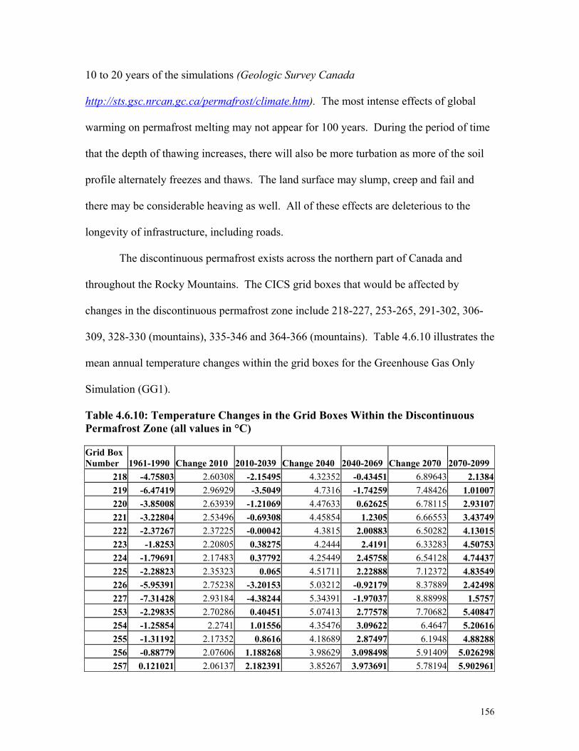
156

10 to 20 years of the simulations (Geologic Survey Canada

http://sts.gsc.nrcan.gc.ca/permafrost/climate.htm). The most intense effects of global

warming on permafrost melting may not appear for 100 years. During the period of time

that the depth of thawing increases, there will also be more turbation as more of the soil

profile alternately freezes and thaws. The land surface may slump, creep and fail and

there may be considerable heaving as well. All of these effects are deleterious to the

longevity of infrastructure, including roads.

The discontinuous permafrost exists across the northern part of Canada and

throughout the Rocky Mountains. The CICS grid boxes that would be affected by

changes in the discontinuous permafrost zone include 218-227, 253-265, 291-302, 306-

309, 328-330 (mountains), 335-346 and 364-366 (mountains). Table 4.6.10 illustrates the

mean annual temperature changes within the grid boxes for the Greenhouse Gas Only

Simulation (GG1).

Table 4.6.10: Temperature Changes in the Grid Boxes Within the Discontinuous Permafrost Zone (all values in °C) Grid Box Number 1961-1990 Change 2010 2010-2039 Change 2040 2040-2069 Change 2070 2070-2099

218 -4.75803 2.60308 -2.15495 4.32352 -0.43451 6.89643 2.1384219 -6.47419 2.96929 -3.5049 4.7316 -1.74259 7.48426 1.01007220 -3.85008 2.63939 -1.21069 4.47633 0.62625 6.78115 2.93107221 -3.22804 2.53496 -0.69308 4.45854 1.2305 6.66553 3.43749222 -2.37267 2.37225 -0.00042 4.3815 2.00883 6.50282 4.13015223 -1.8253 2.20805 0.38275 4.2444 2.4191 6.33283 4.50753224 -1.79691 2.17483 0.37792 4.25449 2.45758 6.54128 4.74437225 -2.28823 2.35323 0.065 4.51711 2.22888 7.12372 4.83549226 -5.95391 2.75238 -3.20153 5.03212 -0.92179 8.37889 2.42498227 -7.31428 2.93184 -4.38244 5.34391 -1.97037 8.88998 1.5757253 -2.29835 2.70286 0.40451 5.07413 2.77578 7.70682 5.40847254 -1.25854 2.2741 1.01556 4.35476 3.09622 6.4647 5.20616255 -1.31192 2.17352 0.8616 4.18689 2.87497 6.1948 4.88288256 -0.88779 2.07606 1.188268 3.98629 3.098498 5.91409 5.026298257 0.121021 2.06137 2.182391 3.85267 3.973691 5.78194 5.902961

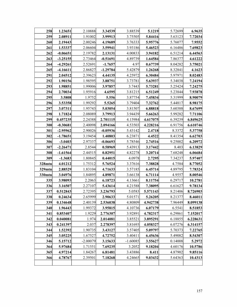
157

258 1.23651 2.10888 3.34539 3.88539 5.1219 5.72699 6.9635259 2.08911 1.91002 3.99913 3.75505 5.84416 5.63123 7.72034260 2.19443 2.00246 4.19689 3.76333 5.95776 5.76077 7.9552261 1.53337 2.06604 3.59941 3.93186 5.46523 6.16486 7.69823262 -0.06651 2.19782 2.13131 4.00833 3.94182 6.51214 6.44563263 -3.25155 2.73464 -0.51691 4.89739 1.64584 7.86377 4.61222264 -4.29261 2.52691 -1.7657 4.97 0.67739 8.04282 3.75021265 -4.16611 2.86827 -1.29784 5.42879 1.26268 8.32841 4.1623291 2.04512 2.39623 4.44135 4.25972 6.30484 5.97971 8.02483292 1.90156 1.98595 3.88751 3.73781 5.63937 5.34038 7.24194293 1.98851 1.99006 3.97857 3.7443 5.73281 5.25424 7.24275294 2.70034 1.95916 4.6595 3.81215 6.51249 5.23844 7.93878295 3.5808 1.9752 5.556 3.87754 7.45834 5.31999 8.90079296 3.53358 1.99292 5.5265 3.79404 7.32762 5.44817 8.98175297 3.07311 1.95743 5.03054 3.81507 6.88818 5.60388 8.67699298 1.71824 2.08089 3.79913 3.94439 5.66263 5.99282 7.71106299 0.457235 2.24388 2.701115 4.15984 4.617075 6.39239 6.849625300 -0.30681 2.40098 2.094166 4.53503 4.228216 6.91756 6.610746301 -2.95962 2.90026 -0.05936 5.43142 2.4718 8.3372 5.37758302 -1.78651 3.19454 1.40803 6.23871 4.4522 8.41354 6.62703306 -3.0403 2.97337 -0.06693 5.78546 2.74516 9.25002 6.20972307 -2.26471 2.8544 0.58969 5.43913 3.17442 8.403 6.13829308 -1.61564 2.44515 0.82951 4.82278 3.20714 7.68248 6.06684309 -1.3683 1.80845 0.44015 4.0978 2.7295 7.34237 5.97407

328mtn 4.01212 1.75312 5.76524 3.37616 7.38828 4.7584 8.77052329mtn 2.88529 1.83104 4.71633 3.57185 6.45714 4.89795 7.78324330mtn 3.04976 1.84895 4.89871 3.66138 6.71114 4.9557 8.00546

335 3.98093 2.2063 6.18723 4.13661 8.11754 6.29717 10.2781336 3.16507 2.27107 5.43614 4.21588 7.38095 6.61627 9.78134337 0.512843 2.72395 3.236793 5.0583 5.571143 8.21406 8.726903338 0.24634 2.65999 2.90633 5.01571 5.26205 8.21377 8.46011339 0.134648 2.40139 2.536038 4.80809 4.942738 7.96449 8.099138340 1.96443 1.99372 3.95815 4.10736 6.07179 6.5541 8.51853341 0.853407 1.9229 2.776307 3.92891 4.782317 6.29861 7.152017342 0.040081 1.974 2.014081 3.85521 3.895291 6.18855 6.228631343 0.241397 2.037 2.278397 3.81693 4.058327 6.07276 6.314157344 1.52392 1.90735 3.43127 3.57405 5.09797 5.70373 7.22765345 3.05225 1.67527 4.72752 3.40411 6.45636 5.49082 8.54307346 5.15712 -2.00079 3.15633 -1.60085 3.55627 0.14008 5.2972364 5.97684 1.71551 7.69235 3.2052 9.18204 4.60176 10.5786365 4.97214 1.84267 6.81481 3.43886 8.411 4.87902 9.85116366 4.78767 2.39501 7.18268 4.24665 9.03432 5.64363 10.4313

158

If the temperatures in degrees Celsius for the grid boxes within the discontinuous

permafrost zone are plotted over time, the warming trend in this zone can clearly be seen

(Figure 4.6.3).

Figure 4.6.3: Temperature Distribution (°C) for Grid Boxes Within Discontinuous Permafrost Zone

Each grid box is represented by a different colour in Figure 4.6.2. It can be easily

seen that the mean annual temperature increases over the four scenarios (1961-1990 base,

2010-2039, 2040-2069, 2070-2099). Mean annual temperatures of 1-2°C characterize the

discontinuous permafrost zone. Table 4.6.11 summarizes the changes that are projected

to take place for the 57 grid boxes within this zone with reference to permafrost stability.

Table 4.6.11 Temperature Changes Within Grid Boxes Located Within Discontinuous Permafrost Zone Scenario Number of Grid Boxes

with Mean Annual Temperature Below 2 °C

Grid Boxes with Mean Annual Temperature Below 2 °C as a Percentage of the Total Grid Boxes

Percent Change in Number of Grid Boxes Between Scenarios

1961-1990 40 70% 2010-2039 23 40% 30% 2040-2069 9 16% 24% 2070-2099 2 4% 12%

- 1 0 - 8 - 6 - 4 - 2 0 2 4 6 8 1 0 1 2

1 9 6 1 - 1 9 9 0 2 0 1 0 - 2 0 3 9 2 0 4 0 - 2 0 6 9 2 0 7 0 - 2 0 9 9

159

As can be seen from this table, 70% of the grid boxes that are completely or

partially within the discontinuous permafrost zone have mean annual temperatures below

2 °C for the 1961-1990 base. According to the CGCM1-GG1 model, by 2010-2039, that

percentage will have dropped to 40%. By 2040-2069, that percentage will have further

decreased to 16%. The mean annual temperature for the grid boxes affected by the

discontinuous zone will have risen to the point that only 4% of these areas will have

temperatures below 2 °C by 2070-2099. Virtually all permafrost will have disappeared

from 96% of this area. The remaining 4% of the grid boxes have projected mean annual

temperatures of 1-1.5°C, which suggests that the permafrost may disappear from these

areas as well. While an analysis of the amount of change between different scenarios

suggests that the loss of permafrost may be progressively less with each temporally

advancing scenario (30% to 24% to 12%), it must be remembered that the permafrost will

come into equilibrium with the ambient temperature at a slower rate than temperature is

changing. Mineral and organic soil act as insulators and slow the rate of permafrost

melting.

4.6.1.2: Bridges

The adaptation costs associated with Canada’s bridge infrastructure are expected

to be low for two reasons. First, in North America, a significant percentage of the

existing bridge infrastructure has deteriorated and is in need of repair or replacement

(Newhook et al, 1997). As a result, most bridges will require repair regardless of climate

change. Second, the national standard for bridge design (CAN/CSA-S6-88) is in the

process of being replaced with a more rigorous code. The new code will require bridges

to be designed to last for 75 years (25 years longer than the present code). Many bridges,

160

especially in British Columbia, are currently being retrofitted to be able to withstand

earthquakes. As the stresses from an earthquake far exceed any building stress that could

result from climate change and the new bridge code utilizes improved materials in

construction, most new bridges will be more than adequately prepared to survive the

influences of climate change. While changes in humidity and temperature have an effect

on concrete and steel, much of the effects of climate change will be absorbed in the cost

of upgrading existing structures to the new standards.

In the United Kingdom in 1990, 30% of bridges were in good condition, 50% of

bridges were in fair condition and 20% of bridges were in poor condition. An estimate of

repair on this bridge condition profile was approximately £10 million, to be spent on 200

bridges over 10 years. Bridges in good condition require an average expenditure of one

quarter of the expenditures on bridges in fair condition. Bridges in fair condition require

an average expenditure of one quarter to one fifth of the expenditures on bridges that are

in poor condition. If bridges are allowed to deteriorate, the expenditures escalate

enormously. It is a geometric, rather than an arithmetic progression in terms of costs

versus condition for bridges. The deterioration of Canada’s infrastructure will necessitate

expenditures on bridges that will likely overshadow any climate change adaptation costs.

Typical bridge replacement costs in the United States and Canada are $500,000 to

$625,000 (Cdn); typical bridge replacement costs in the UK are double this amount.

The effects on capital expenditures for bridges can be subdivided into effects on

inland versus coastal bridges. The increased effects of scour will be sustained as a

maintenance cost. There may be additional costs on bridges with respect to vessel

impacts. This will affect all bridges over water.

161

4.6.1.2.1: Inland Bridges

Inland bridges are not expected to sustain the impact that coastal bridges are

expected to sustain. The impact of climate change in the form of increased loads is small

compared to such factors as earthquake susceptibility. As stated earlier, provincial

bridges in British Columbia are currently in the process of being retrofitted to withstand

seismic activity. The increased strength and durability imposed by earthquake

susceptibility retrofitting far exceeds any cost imposed by climate changes. Most bridges

are over designed; there is sufficient strength in the structure to compensate for additional

wind force, for example. Increasing the wind force by 100%, which is in excess of

predicted levels, will only increase bridge construction costs by 5-10% and only on very

large bridges (Madar Bahkt, personal communication). Most bridges do not have enough

exposed surface area to be affected by wind force. Increased scour due to increased

water flow may have an effect on bridges over water and the addition of gabions or riprap

to stabilize the substructure may be necessary.

4.6.1.2.2: Coastal Bridges

One of the primary impacts of global warming is sea level rise. In Canada, all

provinces and territories have coastal areas except Alberta and Saskatchewan. One

province, Prince Edward Island, is completely surrounded by ocean. The impact on

bridges from sea level rise is twofold. Firstly, the substructure of the bridge will be more

exposed to salt water and, therefore, more subject to the deleterious effects of chloride

ions. The superstructure may be subject to increased salt spray, causing damage. Both

concrete and steel are subject to breakdown by salt action. Concrete spalling and the

corrosion of steel bridge structures result in a shortening of the longevity of the bridge.

Increased spalling and corrosion can be alleviated by increased maintenance (cleaning,

162

painting and repair). Concrete bridges are maintained by washing, patching broken

concrete, replacing corroded expansion joints and drains and the use of electrical

techniques to “pull” the chloride ions from the concrete. When a bridge must be

rehabilitated, it is usually the superstructure that has deteriorated first, not the

substructure. Bridge failure is not usually due to the deterioration of the structure of the

bridge. More often, bridge failure is due to scour; the flow of water around the base of

the structure tends to remove materials from the base and the bridge collapses. Although

there are salt-water effects, the deterioration of bridges is not usually linked to a salt-

water environment. Engineers do not consider a salt-water environment to be as major a

source of bridge deterioration as road de-icing salts for state and provincial bridges.

There may also be minor changes in the amount of deterioration due to changes in the

amount of salt-laden fog in the coastal areas.

Secondly, the superstructure of the bridge may be too low to allow the passage of

vessels underneath. Raising a bridge usually entails the removal of all, or part, of the

bridge deck. This is a major expense, and may be close to the replacement cost for the

entire bridge. In 1958-1959, the Jacques Cartier Bridge over the St.Lawrence River in

Montreal, Quebec was raised from 12.2 metres to 36.5 metres above the water to

accommodate ships passing through the newly constructed St. Lawrence Seaway. This

“bridge raising” was only performed on the section of bridge between piers 9 and 10 and

took 16 months. Thirty jacks with a capacity of 362.87 to 544.3 tons were employed to

raise the bridge to its present level. Temporary bridges were also part of the cost; traffic

was not disrupted (Jacques Cartier and Champlain Bridges Incorporated

http://www.pjcci.ca/English/jacques-cartier/construction.htm). The expense of raising a

163

bridge is the cost of deck replacement plus the installation of jacks between the

substructure and the superstructure. For the Jacques Cartier Bridge, this cost was

$6,698,750 in 1959 for only a small section. It was possible to raise this particular bridge

but, in most cases, the bridge will have to be replaced rather than raised. While there

may be some effect from increased salt spray and increased exposure of the bridge to salt

water, the major cost associated with increased sea level is the raising of the bridge to

accommodate ship passage.

Most of the coastal bridges that will be affected by sea level rise are along the east

coast of the country and were built over the Atlantic Ocean or the St. Lawrence River.

The lower portion of the St.Lawrence River will be affected by sea level changes and the

portion of the river affected by tidal influences may increase. Currently, the brackish

water zone (where salt and fresh water mix) extends between La Pocatière and Île

d’Orléans. Tidal effects may be felt as far south as Trois-Rivières. The topography of

the west coast of Canada does not lend itself to the construction of coastal roads; hence

there are few roads that span inlets from the Pacific Ocean. The coastline of the Arctic

Ocean is sparsely populated and does not have many bridges. There are no major coastal

roads running the length of the Arctic Ocean. A summary of the number of coastal

bridges in the country in given in Table 4.6.12.

Table 4.6.12: Number of Coastal Bridges in Canada Province Coastal Bridges (publicly maintained) 1 Total Number Alberta 0 (no sea coast) British Columbia 52 5 Manitoba 03 New Brunswick 700 (mostly provincial) including causeways4 700 Newfoundland 30 (provincial) 10 (municipal) 5 40 Nova Scotia 1800 (provincial) very few municipal 6 1,800 Ontario 07 Prince Edward Island 300 (provincial) 8 300

164

Quebec 330 (provincial and municipal) 9 330 Saskatchewan 0 (no sea coast) Northwest Territories 010 Nunavut 1011 10 Yukon 012 Total 3,185 1 Bridges maintained by the federal, provincial, regional and local governments 2 Bill Szeto, BC Ministry of Transportation and Highways 3 Manitoba Highways and Transportation; Town of Churchill 4 Neil Gilbert, New Brunswick Department of Transportation (25% of total bridges) 5 Peter Lester, Newfoundland Works, Services and Transportation 6 Tom Gouthro, Nova Scotia Transportation and Public Works (50% of total bridges) 7 Town of Moosonee 8 Ken Hoy, Prince Edward Island Transportation and Public Works (25% of total bridges) 9 based on 10% of total number of bridges in regions of Quebec with coastal areas http://www.mtq.gouv.qc.ca/regions 10 Larry Purka, Northwest Territories Transportation 11 Doug Sitlin, Nunavut Community and Transportation 12 Bernie Cross, Yukon Community and Transportation Services

The total number of bridges in Canada that potentially need to be adapted to a rise

in sea level is approximately 3,185. While it may be possible to utilize jacks or remove

the deck and increase the height of the substructure, this may not always be feasible. The

process is very individual, depending on the bridge design. Bridge replacement is more

costly than bridge jacking but there may not be an alternative. The substructure of many

bridges may not be able to withstand the additional weight, and improvements are often

in order if any bridgework is required. Bridge replacement is likely the most viable

alternative for bridges affected by sea level rise. Ocean-going vessels are increasing in

size and decreasing in maneuverability, and will be expected to navigate into ports and

under bridges with less clearance. The present clearances are not, therefore, excessive.

In order to maintain the present portfolio of bridge infrastructure, approximately 3,185

coastal bridges will require replacement. There may be additional causeways that may

have to be replaced, but this information was not readily available.

165

The replacement cost of bridges is unknown, as the new standard for bridge

construction will be in effect shortly. One study in the United States estimates that $90

billion should be allocated to replace approximately 200,000 bridges (Dunker and Rabbat

1993). If we take the total cost and divide it by the total number of bridges we get the

average cost of $450,000 US per bridge for bridge replacement. At the present exchange

rate of 1.5, this gives a cost of $670,000 Canadian. Estimates from Newfoundland and

Manitoba on the average bridge replacement cost, at the provincial level, are currently

$500,000 and $625,000 ($1.5 billion divided by 8,200 bridges) respectively. The

average cost is therefore approximately $600,000 for a bridge. This appears to be

consistent with the replacement of a variety of bridge sizes. The total cost to replace

3185 coastal bridges affected by climate change at an average cost of $600,000 would

therefore be $1,911,000,000 (see Table 4.6.13).

Table 4.6.13: Coastal Bridge Replacement by Province Province Total Number Replacement Costs ($) Alberta British Columbia 5 3,000,000 Manitoba New Brunswick 700 420,000,000 Newfoundland 40 24,000,000 Nova Scotia 1,800 1,080,000,000 Ontario Prince Edward Island 300 180,000,000 Quebec 330 198,000,000 Saskatchewan Northwest Territories Nunavut 10 6,000,000 Yukon Total 3,185 1,911,000,000

Most of the costs of bridge replacement due to sea level rise will be borne by the

Atlantic Provinces (Figure 4.6.3 and Figure 4.6.4). Nova Scotia is most vulnerable to the

166

rise in sea level caused by climate change; over half the costs of bridge replacement will

fall on this province. Other east coast provinces are much less susceptible.

Figure 4.6.3: Coastal Bridge Replacement by Province by the Year 2100

Figure 4.6.4: Proportion of Coastal Bridge Replacement Costs by Province

A summary of coastal bridge replacement costs for all levels of government is

given by province in Table 4.6.14.

Alberta0%

British Columbia0%

New Brunswick22%

Newfoundland1%

Nova Scotia58%

Prince Edward Island 9%

Quebec10%

Nunavut0%

British ColumbiaNew BrunswickNewfoundlandNova ScotiaPrince Edward IslandQuebec Nunavut Yukon

0

500

1000

1500

2000

2500

3000

3500

British Columbia New Brunswick

Newfoundland Nova Scotia Prince Edward

I l d

Quebec Nunavut Total

Province/Territory

Number

Total Number

167

Table 4.6.14: Coastal Bridge Replacement by Province (Year 2100) Province Total Number Replacement Costs ($) British Columbia 5 3,000,000 New Brunswick 700 420,000,000 Newfoundland 40 24,000,000 Nova Scotia 1,800 1,080,000,000 Prince Edward Island 300 180,000,000 Quebec 330 198,000,000 Nunavut 10 6,000,000 Total 3,185 1,911,000,000 4.6.1.2.3: Bridges Over Water

All bridges over water are built to certain specifications regarding the impact of

vessels on the structures themselves. There must be sufficient strength to withstand a

ship hitting the piers of the bridge. While these incidents are fairly rare, they often have

severe consequences for the bridge structure and lives are often lost when the bridge

breaks apart. According to the report by the American Association of State Highway

Transportation Officials (1991), ship-bridge collisions are likely to increase. Many

bridges are not currently designed to accommodate modern ships, which may exceed 800

feet in length and 100 feet in width. The bridge spans are often too narrow. If this is

coupled with poor visibility, which often accompanies dense rainfall and high winds,

ship-bridge collisions tend to increase in frequency. A bridge substructure that

incorporates narrow spans on the bridge will increase the likelihood of collision under

adverse hydraulic or wind conditions. In 1985, the St.Louis Bridge across the

St.Lawrence near Valleyfield, Quebec was partially destroyed by a freighter that rammed

one of the side spans of the lift bridge, temporarily closing the St.Lawrence Seaway.

There are bridges in the United States that have been hit multiple times in the last 30

years. There are also indications that ship-bridge collisions are increasing. Between

1960 and 1970, there were 0.5 ship-bridge collisions per year. Between 1971 and 1982,

168

there were 1.5 ship-bridge collisions per year. An increase in precipitation and wind

speed with climate change will likely produce a greater number of ship-bridge collisions

per year, with catastrophic life and property loss over the next 100 years.

4.6.1.3: Ditches and drains

The impact of climate change on capital costs for ditches and drains is expected to

be large. The expenditures on ditches and drains are small, however, compared to the

capital expenditures on roads and bridges and the overall costs are likely to be low for

most of the country. The ability of the storm water management system to handle large

flow volumes determines, at least to some degree, the longevity of the road system. The

road surface is only expected to last 15-25 years but this is deceptive. An inadequate

storm water management system will not only wash out, resulting in the loss of the

culverts and destruction of the ditches and drains in the process, but the road over top of,

and adjacent to, the culvert will also disappear. Larger storm water management

facilities may sustain greater adaptation costs, especially if dams or dikes are involved.

4.6.2: Operating Costs

The impact of climate change on operating costs can be broken down into the

impact on roads, bridges, ditches and drains (storm water management systems) and

winter control. Winter control often includes operating costs that may be associated with

bridges, roads and storm water management systems but municipalities do not separate

these different aspects. Winter control is often separated from other operating costs, as it

is a major portion of the budget of municipal, provincial and the federal government in

many parts of the country. From our point of view, it was fortunate that this separation

occurred. Winter control costs are severely affected by changes in climate. The climate

169

variables involved in winter control costs are different from the climate variables that will

affect summer maintenance on the road network and its associated components.

4.6.2.1: Roads

The impact of climate change on road operating costs is expected to fall mainly

on road repair and primarily on paved roads. In order to maintain the integrity of the road

surface and provide for safe movement of a car over the surface, roads must be patched

regularly. Pothole formation occurs when the road surface freezes and thaws, causing

cracking and erosion of the road surface. The road surface is also affected by frost heave

in the more northerly parts of the country. Freeze-thaw cycles result when the

temperature of the roadway moves above and below 0°C; these conditions are not a result

of a severe climate. According to the Transportation Association of Canada

(https://mediant.magma.ca/tacatc/resource/viewDocuments.cfm?ID=16&member=REG)

, there are indications that improvements in tolerance of high temperature rutting and low

temperature cracking can be achieved through the use of different materials such as

recycled tire rubber in asphalt pavements. While some improvements in the tolerance of

pavement to freeze-thaw cycles can be expected, freeze-thaw cycles are critical to the

amount of maintenance and the longevity of the pavement. An approximation of the

number of freeze-thaw cycles across central and southern Canada is given in Table

4.6.14.

Table 4.6.14: Approximate Number of Freeze-Thaw Cycles in Heavily Populated Areas of Canada Grid Box Number 1961-1990 Location

327 30 Central BC 328 63 Central BC 330 45 Central AB 331 30 Central AB 332 25 Central SK 333 36 Central SK

170

334 31 Central SK/MB 363 1 Southern BC 364 52 Southern BC 365 54 Southern BC 367 39 Southern AB/SK 368 42 Southern SK 369 46 Southern SK/MB 370 34 Southern SK 371 37 Northern ON 409 38 Northern/Central ON 410 36 Central ON 411 37 Eastern ON, Southwestern PQ 412 31 Southern PQ 413 59 NB, NS 414 55 NB, NS, PEI 417 0 Southern NF 444 41 Central ON 445 37 Southern ON 446 54 Southern ON

Some of the highest numbers of freeze-thaw cycles are found in the Atlantic

Provinces (except southern Newfoundland), southern Ontario and parts of the interior of

British Columbia. The southern part of British Columbia along the Pacific coast has few,

if any, freeze-thaw cycles. The temperature is simply too high in this area throughout the

winter. The Prairie Provinces do not appear to have as many freeze-thaw cycles.

Although the climate is characterized by severe winters in this area, temperatures do not

tend to hover near freezing. The advent of winter is characterized by a rapid progression

from temperatures above freezing to temperatures below freezing. The Prairie springs

are characterized by a rapid progression of temperatures below freezing to temperatures

above freezing. There is little fluctuation over the late fall, winter and early spring. The

effects of freeze-thaw cycles would be expected to be most severe in Alberta,

Saskatchewan and Manitoba.

171

Roads in the colder, more extreme parts of the country would be expected to

sustain more damage due to frost heave, where the duration of the winter and not the

freeze-thaw cycles may factor more into the road maintenance costs.

4.6.2.2: Bridges

The changes in operating costs for bridges with climate change will arise from

two sources, changes in scour for bridges that are over water and changes in deterioration

due to changes in salt application. There may also be some changes in bridge

deterioration due to changes in ground water salinity changes and changes in vegetation

growth. It is not expected than any other climate factors will have a major impact on the

maintenance costs for bridges. There may be small changes in the amount of concrete

spalling due to changes in diurnal temperature ranges, but bridges are built to compensate

for large variations in temperature. The daily temperature fluctuations have much less

effect on a bridge than the seasonal fluctuations. Unless there is a large increase in the

amount of temperature difference between the winter and the summer, there will be little

effect on bridges. According to Phil Jarrett (Environment Canada, personal

communication), the climate is not getting warmer; rather, the climate is getting less cold.

The impact of climate change on bridge repair and maintenance will arise from

changes in the speed and volume of water that flows past the substructure. Lower water

flow will result in less scour effect for bridge substructures (Madar Bahkt, personal

communication). The bridges over the Great Lakes and the St.Lawrence Seaway Bridges

will likely be a cost saving on the substructure due to reduced maintenance and reduced

bridge failure. In areas that will sustain heavier rainfall, the bridge substructure may be

more subject to failure and more maintenance will be performed in the form of gabions

and riprap.

172

Cost changes due to climate change impact will also result from changes in salt

application. Salt is a major cause of the deterioration of bridges and salt application is

related to temperature and precipitation. Salt is not needed above freezing and is not

effective below -10°C. Salt will spall the concrete and corrode the steel in the bridge.

Current bridge maintenance procedures, such as cathode extraction of chloride ions, may

become more or less necessary depending upon the amount of salt that is applied to the

bridge. Integral abutment bridges have been introduced in the last few years. These

bridges lack the steel expansion joints in the middle of the bridge, thus rendering them

less susceptible to the effects of salt and expensive bridge rehabilitation. A single

expansion joint replacement may cost as much as $50,000 Canadian (Ralph Sholtz,

Regional Municipality of Niagara, personal communication). The use of this new type of

design, which allows for the use of expansion joints only every 100 to 150 metres of

bridge span results in more thermal expansion stress for the bridge structure but less

impact from salt use.

4.6.2.2.1: Salt Application on Bridges

Scour is the greatest cause of bridge failure but salt is the major cause of bridge

deterioration. Unfortunately bridges tend to “ice up” more than road surfaces and more

de-icing chemicals are necessary to ensure that bridges are safe for both vehicles and foot

traffic. There are a number of de-icing chemicals used to melt ice on bridge surface.

Sodium chloride and calcium chloride are usually used to remove ice from road and

bridge surfaces. Acetates, such as calcium magnesium acetate, may be used in place of

the chloride compounds but the cost is considerably higher. Acetate compounds cost

approximately $2,000 per tonne; sodium chloride costs approximately $65 per tonne

(Mittlestaedt, 2001). The chloride compounds are the de-icing chemicals of choice,

173

except for large steel bridges, due to the considerable difference in price. The cost of

repairing bridges affected by road salt corrosion is accepted as part of the cost of

maintaining safe traveling conditions on the bridge. In spite of the lower costs of the

chloride compounds, de-icing chemicals are one of the major costs of road maintenance,

according to the Ontario Ministry of Transportation. At $65 per tonne the costs of road

salt exceed $300 million per year in Canada. A warmer climate will reduce these costs in

the areas of the country where salt is currently used for de-icing. For bridges such as the

Thousand Islands Bridge at Gananoque, Ontario, climatic warming will reduce the direct

costs of de-icing and winter control dramatically. This bridge complex is composed of

two large steel suspension bridges and two smaller bridges. The maintenance costs

exceed $2 million annually for these bridges. Acetate compounds are used on these

bridges and the costs of winter control are high as a result.

Road salt corrodes steel bridges, any exposed steel rebar in concrete bridges,

guard rails, expansion joints in concrete bridges plus lighting fixtures associated with

bridges. Corrosion from road salt will also spall concrete, exposing the steel rebar to salt

damage. Some improvements have been made in salt-induced deterioration of concrete

bridges by changes in the type of concrete that is used, and by using epoxy-coated rebar,

which is salt-resistant. In the new Canada Highway Bridge Design Code, stainless steel

rebar is recommended, which will provide greater protection against bridge deterioration.

Some additional longevity in bridges has been provided by the development of cathode

rehabilitation. This technique will draw the chloride ions from the concrete and may add

10 years to the lifespan of the bridge. It should be pointed out, however, that most of the

bridges in Canada pre-date the development of stainless steel rebar and improved

174

concrete. There have been a few problems with the integrity of the concrete as a result of

the use of cathode rehabilitation. Road salt will likely continue to be a major cause of

bridge deterioration. Toronto alone uses 130,000 tonnes of road salt yearly. The largest

users of road salt include Toronto, Ottawa, Halifax and Quebec City; these cities lie

within a climatic zone where the temperature range in winter permits the melting of snow

using de-icing chemicals. Vancouver uses some salt, but the temperatures are usually too

warm for ice formation (Mittlestaedt, 2001). Other cities, such as Edmonton, Calgary,

Regina, Saskatoon and Winnipeg, are too cold, rendering salt ineffective for much of the

winter. A reduction or increase in the use of road salt as a result of climate change will

make a difference to the operating costs associated with bridges.

4.6.2.3: Ditches and Drains

The impact of climate change on the costs associated with maintaining ditches

and drains and the storm water management system are expected to be very small.

Maintenance of ditches and drains is a very small component of operating costs and these

procedures are often performed at the same time as the regular road inspection and

maintenance. There are indications that changes in the amount of mowing may be

necessary (Palutiko et al, 1997, pg135). It is also possible that there may be changes in

the amount of material that passes through the drains and culverts, resulting in an

increased or decreased need to flush and clean the storm water management system.

Culvert thawing involves ditches and drains maintenance but is usually included as part

of winter control budgets.

4.6.2.4: Winter Control

The impact of climate change on the costs associated with winter control is

substantial. Winter control may be as much as 50% of a municipal road operations

175

budget, depending on the amount of service that the municipality provides. Some cities

clear streets, sidewalks and windrows. The winter control budget for these cities

constitutes a large portion of the funds allocated to roads operations expenditures. Other

cities have no winter control budget. Temperatures rarely reach freezing and snow and

ice formation is consequently not a problem. Winter control costs are therefore related to

both the level of service and the winter conditions. It is reasonable to assume that the

winter control costs will vary to a large degree with the amount of snowfall. This

relationship is somewhat complicated by the distribution of snowfall; it is possible to

have a few large snowfalls during the winter that result in very high winter control costs.

It is also possible to have low winter control costs if the snow is evenly distributed as

frequent, very light snowfalls throughout the winter season. Large snowfalls are

particularly expensive for the municipalities, as cities and towns often do not have the

space to store excess snow. Provincial ministries of transportation often utilize right-of-

ways for snow storage and are able to handle heavy snowfalls more easily.

The costs of winter control vary considerably across the country, which is not

unreasonable considering the variability in climate and the level of services provided for

a vast geographic area. Based on our questionnaire response, costs of winter control may

range from 0 to nearly 50 % of the roads operating expenditures for an individual

municipality. As operating expenses comprise a substantial portion of the roads

operating expenditures, the effect of increases or decreases in such costs as a result of

regional climate change could be substantial. The relationship between winter control

costs can be expected to vary with location, with the level of service provided by the

municipality and with the ability of the individual municipality to levy taxes to pay for

176

these services. Winter control will vary considerably with geography; the City of

Victoria in southern coastal British Columbia has no winter control budget but the City of

Yellowknife in the Northwest Territories could not reasonably be expected to have no

winter control expenditures.

We have initially speculated that there is a linear relationship between winter

control expenditure and total snowfall, per km of roadway, ignoring differences in the

level of service between municipalities. This may be an oversimplification, as we are not

capturing differences in costs associated with different types of roadways. Paved roads

usually accommodate more traffic and have higher plowing, sanding and salting costs

than gravel roads. Highways with higher superelevation (8% versus 6%) must be salted

and sanded more frequently for safety reasons. Paved roadways may also be multi-lane

and the kilometres of road may not reflect the actual amount of road surface. Gravel

roads are usually narrower and require less plowing. Winter control for gravel roads does

not usually include salting. The amount of snowfall is not the only parameter involved in

winter control costs; the distribution of snowfall is critical to the need for snow removal.

Costs depend on the snow pack and accumulation and not just on simple snowfall. In

general, however, municipalities that have more snowfall on their roadways should incur

higher costs, ceteris paribus. This should logically be reflected in empirical analysis of

real world data.

A general relationship of the following structure was examined:

WCi = α0 + β1Sn1 + β2D2i + β3D3i + … + βnDni + ui

WC - winter control expenditure per km of roadway (1996, 1997 or 1998 dollars) n - total annual snowfall, in centimetres, based on Canadian Climate Normals

D - dummy variables that are introduced to take into account location factors that influence costs α - constant β - slope (rate)

177

u - residuals (error)

In order to undertake the above analysis we would normally require a fairly rich

data set, with reliable information on actual winter control operating expenses and

measures of the size of the infrastructure characteristic in question, including the number

of kilometres of roadway, the type of road surface and the level of service for which the

municipality is responsible. Unfortunately, we did not have so rich a data set to work

with. We began with a sample of 98 municipalities. The numbers of kilometres of roads

was available for only 26. In the case of 10 of these 26, there seemed to be glaring

inconsistencies as to the size of expenditures in relation to the number of kilometres of

roadways. We were therefore forced to drop these municipalities from our sample. That

left us with 16 municipalities for which the data seemed reasonable.

We then plotted a scatter diagram of winter control expenditure per km of

roadway against total snowfall per annum in centimetres. As expected, there was a

simple linear relationship between winter control expenditure and total snowfall. We did

note, however, that the data from the City of Yellowknife appeared to be an “outlier.”

What we seemed to have was a group of municipalities that probably face similar

economic conditions and input cost structures with one exception. Unfortunately, we are

unable to carry out the analysis outlined above using dummy variables to capture the

locational differences, as there were not enough data points. We were forced to drop the

anomalous observation on the assumption that the municipalities included in the analysis

are fairly homogeneous from the standpoint of the sorts of input costs they face. We

were then left with 15 data points, displayed in Figure 4.6.5 and noted in Table 4.6.15.

178

Figure 4.6.5: Winter Control Expenditure Versus Annual Snowfall (per km of road)

Table 4.6.15 Winter Control Costs – Selected Municipalities

We can take the information from this figure and table and undertake the simpler

analysis following the general model:

WCi = α0 + β1Sn1 + ui

$0.00$1,000.00$2,000.00$3,000.00$4,000.00$5,000.00$6,000.00

0.00 100.00

200.00

300.00

400.00

500.00

cm per km

Dol

lars

per

km

Municipality Population (1996)

Operations-Winter Control- fraction

Operations-Winter Control-actual

Operations Budget-Total

Kilometres of Roads

Winter Control Expenditure per Kilometre

Snowfall in cm

Terrace 12779 0.17 $334,019.53 $1,941,974.00 130.00 $2,569.38 389.00Quesnel 8468 0.12 $205,492.08 $1,712,434.00 87.00 $2,361.98 189.40Morinville 6226 0.34 $34,346.80 $101,020.00 45.29 $758.37 127.20Spruce Grove 14271 0.28 $46,639.60 $166,570.00 117.50 $396.93 127.20Red Deer 60075 0.20 $237,963.60 $1,189,818.00 366.00 $650.17 125.10Vermilion 3744 0.50 $662,295.50 $1,324,591.00 3806.00 $174.01 106.70Esquimalt 16151 0.02 $25,105.95 $1,394,775.00 47.00 $534.17 46.90Comox 11069 0.02 $12,954.32 $647,716.00 67.00 $193.35 91.40Port Alberni 18468 0.06 $183,128.45 $3,157,387.00 206.00 $888.97 120.50Victoria 73504 0.00 $0.00 $13,665,813.00 259.00 $0.00 46.90Richmond 1422 0.03 $434,561.61 $14,485,387.00 593.00 $732.82 32.80Revelstoke 8047 0.28 $472,743.04 $1,688,368.00 99.00 $4,775.18 445.30Pont-Rouge 4676 0.45 $314,665.11 $695,700.00 94.15 $3,342.17 337.00Digby 2199 0.35 $49,247.80 $140,708.00 30.60 $1,609.41 283.30Kentville 5551 0.27 $118,709.01 $439,663.00 47.40 $2,504.41 329.50

179

WC - winter control expenditure per km of roadway (1996, 1997 or 1998 dollars) Sn - total annual snowfall, in centimetres, based on Canadian Climate Normals α - constant β - slope (rate) u - residuals (error) It should be noted that any conclusions drawn are applicable to municipalities

similar to those in the data set, from the standpoint of input costs.

The fitted model is expressed as follows:

ŴCi = -326.7809 + 9.4321Sn1

265.4963 1.1676

t=(-1.23) 08

These results from the regression equation indicate that a one-centimetre increase

in total annual snowfall leads to a $9 per km increase in winter control costs. Indeed as

this is averaged data, it might be sensible to take the 95 percent upper confidence limit of

the estimate, which is $11.95. That is, we are 95 % confident that one-centimetre of

snowfall leads to $12 per km increase in winter control costs. The coefficient estimate

on the intercept term is not statistically different from zero, which agrees with our

intuition that cities that have no snowfall incur no winter control costs.

In order to extrapolate this relationship and produce an indication of costs

resulting from a change in climatic conditions, it is necessary to utilize the climate

scenario projections provided by CGCM1 GG1. Unfortunately, the information provided

by CGCM1 is spatially and temporally averaged and does not provide exact information

on changing snowfall patterns at a coarse or fine (local) level. Information on snowfall

can only be projected from CGCM1 GG1 on the basis of monthly precipitation that falls

when the mean temperature is below 0°C. Projected global average warming will be

accompanied by significant regional variations in warming and shifts in precipitation

180

belts. Climate models generally predict greater warming than the global average at

middle to high latitudes, including Canada, and a greater warming in winter than in

summer at middle to high latitudes. More winter precipitation at mid latitudes is

predicted but there are wide differences on changes in summer precipitation.

A simulation of the present day distribution of precipitation, cloudiness, soil

moisture and ice and snow amounts is a necessary but not sufficient condition for reliable

simulation of regional changes in adaptation costs. Many important processes, such as

cloud development, precipitation and land surface hydrological changes, occur at scales

finer than the grid resolution of climate models and therefore cannot be adequately

represented. The information that is currently available allows only a rough estimation of

the impact of climate change.

At present, global climate models seem to indicate that:

1. In general, winters will be 3-5°C warmer in the south and 10-15°C warmer in the

Arctic; summers will be warmer by 2°C in the south and 3°C in the Arctic.

2. Storm tracks would be displaced northward increasing Arctic precipitation; snow

seasons would be shorter in the Arctic but snow totals and spring runoff might be greater.

There are two approaches to calculating winter control costs. We can think in

terms of climate change analysis as trading climates. For example, by 2030 enhanced

greenhouse warming is expected to give Toronto the climate of Pittsburgh in the 1980s,

Sudbury that of Cleveland, Winnipeg that of Minneapolis, Charlottetown that of Boston,

Edmonton that of Cheyenne, Wyoming and Vancouver that of San Francisco.

Consequently, by 2030 we might reasonably expect municipalities in southern British

Columbia to have little or no annual snowfall, those in southern Alberta to have about 20

181

percent less total snowfall, and those in the southern Maritimes to have about two-thirds

less snowfall. Based on these rough generalizations, figures for expected expenditures

for winter control were calculated using the above regression equation. The results are

displayed in Table 4.6.16.

Table 4.6.16: Projected Cost Changes for Winter Control to 2030

On the basis of intuition, these results seem reasonable. The cost projections for

winter control given above are consistent with other information about global warming.

Global warming should result in cost savings for winter control, provided the magnitude

of the temperature increase overshadows the increase in precipitation resulting from the

acceleration of the hydrologic cycle. The above calculations based on the estimated

regression suggest that for the municipalities given in Table 4.6.16, the expenditure on

winter control can be expected to go down. Global warming should lead to a reduction in

snowfall for most of Canada. Projected changes in winter temperatures and snowfall are

given in the tables in Appendices 4.6.2 and 4.6.3. However, as to how these projections

could be used to simulate future costs of adaptation remains a subject for future research.

MunicipalitySnowfall in cm

Expected Snowfall 2030

Expected Expenditure 2030 per km Fitted Value Difference

Terrace 389.00 310.00 $2,597.17 $3,342.31 -$745.14Quesnel 189.40 150.00 $1,088.03 $1,459.66 -$371.62Morinville 127.20 100.00 $616.43 $872.98 -$256.55Spruce Grove 127.20 100.00 $616.43 $872.98 -$256.55Red Deer 125.10 100.00 $616.43 $853.17 -$236.75Vermilion 106.70 85.00 $474.95 $679.62 -$204.68Esquimalt 46.90 0.00 -$326.78 $115.58 -$442.37Comox 91.40 0.00 -$326.78 $535.31 -$862.09Port Alberni 120.50 100.00 $616.43 $809.79 -$193.36Victoria 46.90 0.00 -$326.78 $115.58 -$442.37Richmond 32.80 0.00 -$326.78 -$17.41 -$309.37Revelstoke 445.30 350.00 $2,974.45 $3,873.33 -$898.88Pont-Rouge 337.00 100.00 $616.43 $2,851.84 -$2,235.41Digby 283.30 100.00 $616.43 $2,345.33 -$1,728.90Kentville 329.50 100.00 $616.43 $2,781.10 -$2,164.67

182

4.6.3: Directions for Future Research In this report we have concentrated on the adaptation costs for roads in the following

categories:

1. For northern Canada we have looked at the adaptation costs involved in

converting winter/ice roads to all weather roads (a capital cost). We have also looked at

the capital costs for roads in dealing with the loss of permafrost.

2. For the coastal areas of Canada we have looked the capital costs for bridge

replacement.

3. For road maintenance we have looked at winter control costs and road repair

costs.

Based on our preliminary research, there are still a number of areas that need to be

addressed in so far as climate adaptation costs are concerned.

4.6.3.1: Roads

Road capital and maintenance costs need to be addressed in greater detail. One

could purchase digital road data from Natural Resources Canada’s Centre for

Topographic Information as a series of CD ROMs (http://maps.nrcan.gc.ca/). This

digital road information, which is available as a series of 1:50,000 maps, is called the

Updated Roads Network (URN) and is available for sections of the country. The data are

available as ArcView shape files, which are compatible with our GIS. At the present

time, only a small portion of the country has been completed. The cost per CD ROM is

approximately $300 and the coverage is fairly detailed. The Niagara Peninsula, for

example, is covered by five CD ROMs (five topographic sheets), which would cost

$1500. This is only a small portion of the country (12 small census subdivisions). While

the detail in the urban areas may not be sufficient for climate change adaptation analysis,

183

these maps may be useful for the less populated areas of the country.

Many of the costs associated with climate change adaptation have been evaluated

without consideration for the type of road, although we know that the activities associated

with paved roads and other types of roads are different. Our data have shown that about

50% of all roads in Canada are gravel roads. It would be appropriate to determine

whether there are differences in costs associated with the different types of roads. We

expect that gravel roads would be situated largely in northern communities or in southern

rural communities. The impact of climate change adaptation for roads across the country

may be quite different on this basis alone.

The impact of changes in avalanches may result in greater or lesser costs for road

construction and maintenance. At present, snow sheds and tunnels are used to deflect

snow from the roadway, thus avoiding both the maintenance costs of clearing large

amounts of snow and the possibility of vehicles being buried and lives lost. More or

fewer avalanches may result from the changes in climate parameters producing specific

snow and temperature conditions. This may increase or decrease the need to put

protective structures on roads in the mountainous areas where avalanches are common.

Permafrost monitoring has been ongoing for many years in the Arctic, particularly

in the discontinuous permafrost zone. A more detailed examination of the impact of

permafrost loss on the interaction between permafrost and roads is warranted. The results

of a recent conference in Whitehorse (March, 2001) have underlined the magnitude of the

changes. The impact of climate change for roads, in terms of both permafrost and

winter/ice roads, is expected to be large.

4.6.3.2: Bridges

Bridge information is also available as part of the URN digital data. As in roads,

184

the data may be too coarse for analysis of the urban areas but these data may be suitable

for analyzing the rural and northern areas. In addition, it was discovered that the

definition of a bridge was quite variable from one province to the next. In Alberta, a

bridge was any structure spanning over 1.8 m; in Newfoundland, a bridge was any

structure spanning over 6 m. The data were collected without considering the differences

in definition; consequently the tallies for different parts of the country may be over or

under estimated.

Changes in bridge construction and replacement as a result of ship-bridge

collisions induced by climate change should be examined. Changes in visibility resulting

from climate change plus water level rise or fall may have an impact on the number of

times that ships hit bridges over a year. Increased ship-bridge collisions increase the

number of bridge replacements and may require that the bridge designs be changed in the

future. Larger bridge spans may be required to avoid collisions and stronger piers may

have to be built to withstand the collision with a ship. Ship-bridge collisions often result

in both loss of life and heavy property damage.

The effect of road salt on winter control costs and on bridge maintenance have yet

to be determined. The use of road salt is determined by a temperature minimum and

maximum; the use of road salt is not a simple relationship with temperature.

Precipitation also factors heavily into the use of de-icing chemicals. Temperatures below

0°C do not result in increased use of road salt if there is no precipitation. The application

of de-icing chemicals involves a direct cost, as part of winter control costs, and an

indirect cost, as part of bridge repair, rehabilitation and replacement.

4.6.3.3: Storm Water Management Systems

At present, we have no handle on the costs of adaptation for storm water

185

management systems. Larger amounts of precipitation would be expected to result in

increased costs for larger culverts, deeper ditches and larger storm water detention ponds.

Large water management structures, such as dams, must also be taken into consideration.

These structures are identified by the URN digital database and further analysis may be

considered for these structures using a digital database. The costs of failure for the

current storm water management systems must also be considered. Although the cost of

a larger culvert is small, the cost of installing a larger culvert is large; sections of road

must be removed, the new culvert installed and the road replaced after. This must be

weighed against the probability of any particular section of road washing out due to

insufficient culvert size.

4.6.4: Summary

1. There may be changes in the number of freeze-thaw cycles. A change in freeze-

thaw cycles is more likely to occur in the heartland with fewer cycles on the west

coast. An overall increase of approximately 5°C is expected to occur,

accompanied by an increase of approximately 10% in precipitation.

2. The distribution of roads and bridges between the provincial and local

governments is quite variable across the country. In Ontario, the regional

government assumes much of the responsibilities for road, bridge and storm water

management system construction that would otherwise be handled by the

province. Other provinces, such as British Columbia, also have a two-tier local

government system. Both the municipal and regional levels of government

handle roads.

186

3. About two-thirds of all roads in Canada are under municipal jurisdiction, about a

quarter are under provincial and the rest are under Federal jurisdictions.

4. Roadways are fairly consistent in their design standards as well. Most provinces

use the Transportation Association of Canada (TAC) Geometric Design Guide for

Canadian Roads. There are also guides specific to each province, which often

exist to accommodate special considerations for climate within the province.

5. About 50 percent of all roads in Canada are gravel roads; about a third are paved

roads.

6. The standards for bridge design are fairly consistent across the country, with the

Canadian Standards Association guide, CAN/CSA-S6-88, used in most provinces.

7. Storm water management system guidelines are very diverse across the country.

In most provinces, the design of the drainage system and the level of protection

provided for the associated road depend upon the type of road. Major highways

have more protection against flooding than local roads.

8. A single bridge estimate, which is usually performed before any work is

undertaken, may cost $15,000.

9. Climate affects both capital and operating expenditures. Climate and other

environmental factors constitute one component of the deterioration of roads,

bridges and storm water management systems; the impact of human activities is

the other.

10. The road system in British Columbia, particularly the bridges, is already over-

designed for climate factors, as considerations for seismic activity must be taken

into account already. In the Northwest Territories, considerations for the

187

behaviour of permafrost add almost 50% to the cost of road building per km. A

road built on permafrost costs approximately $500,000 per km to construct; a road

on non-permafrost costs approximately $350,000 per km to construct in the

Northwest Territories.

11. Freeze-thaw cycles and frost heave (temperature effects on soil moisture) require

specific depths of well-drained materials below the road surface to prevent the

deleterious effects of these climatic effects on the roadbed.

12. The highway expenditures in Canada vary across the country. The lowest

expenditures per kilometre of road are found in the Prairie Provinces and the

Atlantic Provinces. British Columbia, Ontario and Quebec have the highest

expenditures per kilometre. These provinces also have high percentages of paved

roads. The percentage of paved roads varies from a low of 5% in the territories

(Yukon, Northwest Territories and Nunavut) to a high of 78% in Quebec. The

Prairie Provinces generally have a low percentage of paved roads. The provincial

expenditures per vehicle do not vary as much as the expenditures per kilometre of

road. Some of the differences in provincial road expenditures may be due to

higher traffic volumes and the increased wear and tear on the road. This is not the

only explanation for the differences.

13. Bridges, compared to other structures, are exposed to the most adverse

environments of loading and climatic change. The climatic loads that must be

considered in bridge design include water loads, ice loads, scour, stream

instability, temperature effects, wind effects, frost effects, groundwater effects

188

and soil properties. All of these factors contribute to the cost of bridge

construction.

14. About 75 percent of bridges in Canada are old and will require replacing anyway.

When they are replaced using the new higher standards, these bridges will be

over-dimensioned and will not need any further adaptation to climate change.

Therefore the climate change adaptations costs will be near zero for bridges.

15. Coastal bridges will need to be replaced due to sea level rises, as it is cheaper to

replace than to raise bridges. The average cost of a bridge is $600 000. The total

cost of replacing over 3000 bridges is estimated to about be $2 billion.

16. There are about 10 000 km of ice roads; most of these are in Ontario and Quebec.

Therefore these two provinces will incur the highest adaptation costs for ice

roads.

17. All weather roads are considerably more expensive to build and maintain. In

northern Ontario, construction of an all-weather road will cost at least $85,000 per

km plus bridges. An average bridge for an all weather road in Ontario will cost

between $65,000 and $150,000 per bridge.

18. If, by the year 2100, all of the winter/ice roads that will no longer be in use are

replaced with all weather roads, and 50% of the winter/ice roads that have

restrictions placed on them are replaced with all weather roads, the number of

kilometres of roads that will require replacement will be about 10,000 km, costing

$908 million.

189

References:

Adams, Christopher R. Impacts of Temperature Extremes Cooperative Institute for Research in the Atmosphere http://www.esig.ucar.edu/socasp/weather1/adams.html Alberta Infrastructure, 1999/2000 Annual Report American Association of State Highway Transportation Officials (AASHTO) (1991) Guide Specification and Commentary for Vessel Collision Design of Highway Bridges Vol I: Final Report. Feb, 1991 Washington: AASHTO. Andra-Warner, Elle, Bringing a Better Quality of Life to Northern Ontario, Bear Country (in-flight magazine of Bearskin airlines) http://www3.sympatico.ca/dennis.catania/Winter_Road.htm British Columbia Ministry of Transportation and Highways, Annual Report 1999-2000. Cohen, Stewart (1997) Mackenzie Basin Impact Study (MBIS) Final Report: Summary of Results http://www.msc-smc.ec.gc.ca/GEWEX/mbis.html Dunker, K.F. Rabbat, B.G.(1993). Why America’s bridges are crumbling. Scientific American, March: 62-72. Environmental Protection Agency, (1998) The Regional Impacts of Climate Change – IPCC – North America. Lonergan, S.C., R.J. DiFrancesco, and M.K. Woo (1993. "Climate Change and Transportation in Northern Canada: An Integrated Impact Assessment". Climatic Change, Vol. 24, pp.331- 351) Mittlestaedt, Michael (2001). Tests Show Sewer Water as Salty as the Ocean. The Globe and Mail, March 29, 2001. Newhook, John P. Mufti, Afti A. MacDonnell, Ralston E. (1997). Steel-free Concrete Bridge Deck - Innovation and Application http://www.mgnet.ca/interoadfed.html Ontario Ministry of Northern Development and Mines (1999), News Release December 20, 1999- 287 Ontario Ministry of Transportation (1991) Ontario Highway Bridge Design Code 3rd Edition. Palutikof, J.P., Subak, S. and Agnew, M.D. (eds) (1997) Economic Impact of the Hot Summer and Unusually Warm Year of 1995 UK Department of the Environment.

190

Road and Transportation Association of Canada (1987), Roadway Infrastructure Study (updated 1999). Road and Transport Association of Canada (1990). Canada’s Roadway Infrastructure: Selected Facts and Figures. Saskatchewan Executive Council News Release Federal-Provincial – 167, April 11, 1995 http://www.gov.sk.ca/newsrel/1995/04/11-167.html Saskatchewan Highways and Transportation News Release 1-9730, November 19, 1997 http://www.inac.gc.ca/nr/prs/s-d1997/1-9730.html) St.Lawrence River – Lake Ontario Plan of Study Team September (1999). Plan of Study for Criteria Review In The Orders of Approval For Regulation of Lake Ontario – St.Lawrence River Levels and Flow, International Joint Commission. http://www.ijc.org/boards/islrbc/pos/studiese.html. Tabler, R. (1994). Design Guidelines for the Control of Blowing and Drifting Snow. Washington, DC: Strategic Highway Research Program NRC SHRP-H-381. Theodor, Nicolas C. and Al-Bazi, George. (1997). Manual of Standard Short-Span Steel Bridges, Ontario Ministry of Transportation Structural Office. Transportation Association of Canada (1991) Highways in Canada 1991 Report. Transportation Association of Canada (1995) Transportation in Canada: A Statistical Overview. Transportation Association of Canada (1996) Utilization of Recycled Tire Rubber in Asphalt Pavements https://mediant.magma.ca/tacatc/resource/viewDocuments.cfm?ID=16&member=REG), Transwest Mining Systems Inc. (1998) Long Haul for Diamonds in the Rough Winter. Warrick, R.A., LeProvost, . Meier,C.M.F. Oerlemans,J. and Woodworth,P.L. (1996). Changes in Sea Level in Climate Change 1995: The Science of Climate Change. Contribution of Working Group I to the Second Assessment Report of the Intergovernmental Panel on Climate Change, Cambridge, UK:Cambridge University Press. Website: http://www.iaw.com/~falls/bridges.html Website: Geologic Survey Canada http://sts.gsc.nrcan.gc.ca/permafrost/pfmapheg2.jpg Website: Geologic Survey Canada http://sts.gsc.nrcan.gc.ca/permafrost/distribution.htm

191

Website: Geologic Survey Canada http://sts.gsc.nrcan.gc.ca/permafrost/pfmacval.jpg Website: Geologic Survey Canada http://sts.gsc.nrcan.gc.ca/permafrost/climate.htm Website: Jacques Cartier and Champlain Bridges Incorporated, http://www.pjcci.ca/English/jacques-cartier/construction.htm Website: Ministère des Transports du Québec, http:www.mtq.gouv.qc.ca/regions Website: Nova Scotia Transportation and Public Works http://www.gov.ns.ca/tran/whoweare/tpwglance.stm Website: Ontario Ministry of Transportation http://www.mto.gov.on.ca/english/engineering/drainage/section9.htm Website: Ontario Ministry of Transportation, http://www.mto.gov.on.ca/english/about/quickfacts.htm). Website: Ontario Ministry of Transportation, http://www.mto.gov.on.ca/english/engineering/drainage/section10.htm#rational Website: Saskatchewan (Yorkton) http://www.touryorkton.com/about_body.html Website: Saskatchewan Highways and Transportation, http://www.highways.gov.sk.ca/travellers_information/ice_roads.htm Website: Transport Canada, A Historical Look at the Federal Government’s Involvement in Highway Infrastructure http://www.tc.gc.ca/pol/en/Report/Highway_Historical _Look/Chapter2.htm Website: Woodmoor The International Ice Bridges to Canada http://www.sault.com/woodmoor/news/bridge.html Website: Yukon Community and Transportation Services http://www.gov.yk.ca/facts.html#TRANSPORTATION & COMMUNICATIONS

192

Appendix 4.6.1: Standards for Ice Road Use – White Ice WHITE ICE - Layers of the ice may have formed from melting snow or slush and is white to opaque in appearance. Normally associated with river crossings.

Thickness in centimetres Equivalent inches Load-pounds Load - kg

15 6 1,482 673

20 8 2,635 1,196

25 10 4,117 1,868

30 12 5,929 2,690

35 14 8,070 3,662

40 16 10,540 4,782

45 18 13,340 6,053

50 20 16,469 7,473

55 22 19,927 9,042

60 24 23,715 10,760

65 26 27,832 12,629

70 28 32,279 14,646

75 30 37,055 16,813

80 31 42,160 19,130

85 33 47,595 21,596

90 35 53,359 24,211

95 37 59,452 26,976

100 39 65,875 29,890

105 41 72,627 32,954

110 43 79,709 36,167

115 45 87,120 39,530

120 47 94,860 43,042

125 49 102,930 46,703

130 51 111,329 50,514

(http://www.highways.gov.sk.ca/travellers_information/ice_roads.htm)

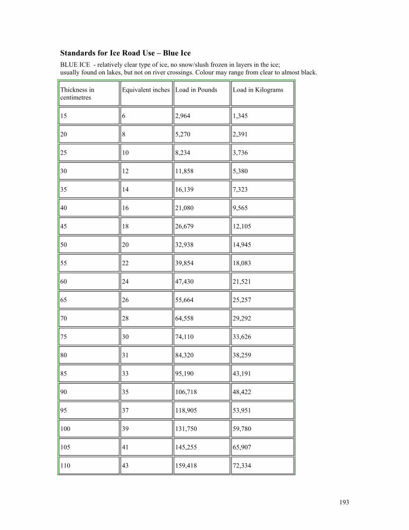
193

Standards for Ice Road Use – Blue Ice BLUE ICE - relatively clear type of ice, no snow/slush frozen in layers in the ice; usually found on lakes, but not on river crossings. Colour may range from clear to almost black.

Thickness in centimetres

Equivalent inches Load in Pounds Load in Kilograms

15 6 2,964 1,345

20 8 5,270 2,391

25 10 8,234 3,736

30 12 11,858 5,380

35 14 16,139 7,323

40 16 21,080 9,565

45 18 26,679 12,105

50 20 32,938 14,945

55 22 39,854 18,083

60 24 47,430 21,521

65 26 55,664 25,257

70 28 64,558 29,292

75 30 74,110 33,626

80 31 84,320 38,259

85 33 95,190 43,191

90 35 106,718 48,422

95 37 118,905 53,951

100 39 131,750 59,780

105 41 145,255 65,907

110 43 159,418 72,334

194

115 45 174,240 79,059

120 47 189,720 86,083

125 49 205,860 93,406

130 51 222,658 101,028

195

Appendix 4.6.2: Winter Temperatures 1961-1990 (Baseline) GRID BOX NUMBER

1961-1990 NOV

1961-1990 DEC

1961-1990\JAN

1961-1990FEB

1961-1990MAR

1961-1990APR

MEAN TEMP 1961-1990

183 -15.09 -21.11 -26.27 -28.12 -22.98 -14.40 -21.33184 -14.99 -21.65 -27.39 -28.16 -20.75 -10.85 -20.63185 -16.46 -22.55 -28.19 -28.92 -21.27 -10.84 -21.37186 -17.00 -22.52 -27.85 -29.70 -24.84 -15.64 -22.92187 -16.70 -22.16 -26.77 -28.16 -24.41 -15.56 -22.29188 -16.72 -21.80 -25.65 -26.77 -23.43 -15.19 -21.60189 -16.91 -22.07 -25.31 -26.84 -23.19 -15.20 -21.59218 -11.15 -18.81 -21.53 -21.08 -13.41 -6.31 -15.38219 -11.24 -19.27 -22.91 -23.93 -18.21 -10.11 -17.61220 -6.97 -18.91 -22.76 -21.33 -13.41 -5.63 -14.84221 -7.17 -19.51 -23.52 -21.82 -13.37 -4.49 -14.98222 -6.66 -19.35 -23.46 -21.44 -12.57 -3.18 -14.44223 -7.68 -19.04 -22.78 -20.57 -11.85 -2.57 -14.08224 -8.26 -19.65 -22.72 -20.03 -11.76 -2.81 -14.20225 -5.19 -20.06 -23.13 -20.82 -13.06 -4.47 -14.46226 -9.64 -21.62 -25.77 -26.14 -21.89 -11.96 -19.50253 -3.61 -10.09 -11.68 -13.30 -10.03 -5.51 -9.04254 -1.70 -9.37 -11.55 -12.01 -8.37 -4.07 -7.84255 -1.56 -10.21 -12.97 -13.02 -9.00 -4.15 -8.49256 -1.40 -10.89 -14.38 -13.80 -9.25 -3.73 -8.91257 -0.78 -10.12 -15.62 -13.99 -8.98 -2.26 -8.62258 -0.33 -9.69 -16.40 -14.01 -8.19 -1.04 -8.28259 -0.30 -11.08 -17.05 -14.00 -6.74 0.03 -8.19260 -0.78 -12.02 -17.09 -14.24 -6.41 0.18 -8.39261 -0.25 -11.18 -17.72 -15.27 -7.87 -1.13 -8.90262 -0.95 -13.58 -19.19 -17.39 -10.42 -3.57 -10.85263 -4.43 -17.89 -21.58 -21.99 -16.65 -9.56 -15.35270 0.15 -2.09 -6.24 -13.28 -13.98 -10.28 -7.62271 -2.68 -15.34 -22.30 -24.83 -22.52 -14.06 -16.95272 2.14 -1.01 -4.09 -9.42 -11.68 -9.27 -5.55295 0.85 -2.49 -10.18 -10.02 -4.47 0.07 -4.37296 0.67 -5.04 -11.76 -10.78 -4.65 0.57 -5.17297 0.63 -4.51 -13.83 -12.46 -5.95 -0.45 -6.10298 0.12 -8.35 -17.16 -15.05 -8.36 -1.64 -8.41299 -0.44 -11.97 -19.46 -17.24 -10.26 -3.11 -10.42300 -0.99 -14.45 -20.24 -18.22 -11.60 -4.38 -11.65301 -1.55 -16.57 -22.66 -23.59 -18.78 -9.97 -15.52305 3.50 -0.85 -4.85 -13.27 -13.89 -8.79 -6.36306 -0.05 -12.46 -19.13 -21.48 -18.57 -10.65 -13.72

196

307 -0.51 -11.71 -16.52 -18.06 -15.79 -9.55 -12.02308 -0.19 -10.92 -15.70 -16.84 -14.09 -8.44 -11.03309 0.40 -9.64 -16.55 -17.87 -14.01 -7.89 -10.93335 0.18 -9.76 -15.21 -12.80 -5.45 1.29 -6.96336 0.35 -9.08 -15.15 -13.32 -7.59 -0.97 -7.63337 0.67 -10.00 -18.52 -18.79 -15.05 -7.09 -11.46338 0.82 -9.99 -17.66 -19.15 -15.36 -7.73 -11.51339 1.07 -8.91 -17.38 -19.06 -15.31 -7.68 -11.21340 0.92 -5.38 -13.61 -14.06 -10.43 -3.98 -7.76341 0.39 -7.23 -14.55 -15.04 -11.12 -4.87 -8.74342 -0.35 -8.81 -15.49 -15.93 -11.68 -5.42 -9.62343 0.05 -8.05 -14.97 -15.52 -11.27 -5.44 -9.20371 1.35 -5.52 -11.25 -9.74 -3.98 2.26 -4.48372 1.32 -4.91 -11.93 -10.39 -4.91 0.22 -5.10373 1.48 -3.70 -11.56 -10.73 -5.51 0.06 -4.99374 1.69 -2.95 -10.55 -10.61 -5.73 0.48 -4.61375 1.70 -1.70 -9.51 -10.23 -5.99 0.04 -4.28376 1.36 -1.31 -9.04 -10.39 -6.72 -0.98 -4.51377 1.08 -1.89 -9.62 -10.79 -7.30 -1.60 -5.02378 1.47 -1.24 -9.03 -10.22 -7.08 -1.73 -4.64379 6.00 2.66 -0.65 -2.53 -2.90 -0.84 0.29411 2.58 0.37 -2.98 -6.60 -2.71 1.64 -1.28412 2.73 0.58 -2.12 -5.74 -2.38 1.39 -0.92

Winter Temperatures 2010-2039 GRID BOX NUMBER

2010-2039 NOV

2010-2039 DEC

2010-2039JAN

2010-2039FEB

2010-2039MAR

2010-2039APR

MEAN TEMP 2010-2039

183 -12.50 -18.84 -22.53 -22.63 -18.34 -10.09 -17.49184 -11.39 -19.74 -23.00 -22.17 -15.91 -7.20 -16.57185 -12.96 -20.86 -24.22 -22.79 -15.90 -6.68 -17.23186 -13.77 -20.94 -25.06 -24.31 -19.47 -11.57 -19.19187 -13.87 -20.23 -24.87 -24.35 -19.24 -11.77 -19.06188 -13.85 -19.52 -23.59 -23.94 -19.14 -12.26 -18.72189 -14.30 -19.21 -23.33 -24.19 -19.62 -12.91 -18.92218 -8.24 -16.07 -18.37 -16.49 -9.71 -4.16 -12.17219 -7.75 -16.49 -19.05 -18.34 -13.78 -7.50 -13.82220 -4.39 -16.15 -19.16 -15.99 -9.50 -3.36 -11.42221 -5.35 -17.12 -19.93 -16.78 -9.59 -2.28 -11.84222 -4.33 -17.38 -20.60 -17.08 -9.20 -1.40 -11.66223 -5.59 -17.08 -20.80 -17.01 -8.93 -0.80 -11.70224 -6.19 -17.20 -20.85 -17.27 -9.10 -1.06 -11.94225 -2.32 -16.30 -21.32 -18.28 -10.32 -2.56 -11.85226 -5.64 -18.04 -23.18 -23.56 -18.58 -10.59 -16.60

197

253 -1.04 -6.97 -9.66 -9.81 -7.27 -4.01 -6.46254 -0.04 -6.07 -9.66 -8.80 -5.68 -2.42 -5.45255 -0.27 -7.24 -11.32 -9.89 -6.28 -2.38 -6.23256 -0.20 -8.04 -12.81 -10.90 -6.70 -1.81 -6.74257 0.22 -7.10 -13.75 -11.32 -6.52 -0.59 -6.51258 0.54 -6.25 -14.27 -11.26 -5.58 0.30 -6.09259 -0.21 -9.09 -15.23 -11.58 -4.32 1.85 -6.43260 -0.29 -9.85 -15.12 -11.83 -4.47 1.93 -6.61261 0.85 -6.80 -15.81 -13.19 -5.78 -0.03 -6.79262 0.59 -7.80 -17.48 -15.40 -8.52 -1.86 -8.41263 -1.23 -13.56 -19.57 -19.72 -13.47 -7.09 -12.44270 2.31 0.61 -0.90 -2.46 -3.51 -2.96 -1.15271 0.31 -10.46 -16.91 -19.85 -15.40 -10.49 -12.13272 4.05 1.08 -0.90 -2.08 -3.06 -2.86 -0.63295 1.54 -0.53 -7.01 -7.31 -2.43 1.10 -2.44296 1.51 -2.15 -9.16 -8.30 -2.78 1.69 -3.20297 1.31 -1.16 -10.79 -10.40 -4.09 0.29 -4.14298 0.97 -3.31 -14.39 -13.18 -6.56 -0.45 -6.15299 0.72 -6.13 -16.95 -15.04 -8.37 -1.62 -7.90300 0.60 -8.47 -17.87 -15.52 -9.38 -2.70 -8.89301 0.61 -10.59 -19.67 -19.67 -14.95 -8.40 -12.11305 5.60 1.43 -0.69 -2.85 -4.86 -3.60 -0.83306 1.22 -6.90 -16.04 -17.25 -13.38 -8.34 -10.11307 0.66 -7.16 -14.07 -14.13 -10.54 -7.00 -8.70308 0.66 -6.95 -13.75 -13.66 -10.00 -6.38 -8.35309 0.90 -5.84 -14.77 -15.78 -12.17 -7.14 -9.13335 1.90 -5.54 -12.57 -10.12 -3.68 2.58 -4.57336 1.86 -4.40 -12.49 -10.45 -4.99 0.45 -5.00337 2.14 -3.78 -15.29 -15.06 -11.37 -5.09 -8.07338 2.36 -4.05 -14.97 -15.00 -11.90 -6.02 -8.26339 2.34 -3.69 -15.40 -15.08 -12.32 -6.55 -8.45340 1.90 -1.82 -11.45 -10.86 -7.85 -2.66 -5.46341 1.21 -3.90 -12.39 -12.06 -8.51 -3.91 -6.60342 0.53 -5.92 -12.86 -12.95 -8.80 -4.49 -7.41343 0.79 -4.67 -12.36 -12.63 -8.39 -4.20 -6.91371 3.21 -2.44 -8.36 -7.34 -1.86 4.22 -2.10372 2.88 -2.07 -8.46 -8.19 -2.90 1.86 -2.81373 3.08 -0.69 -8.12 -8.47 -3.47 0.80 -2.81374 3.19 -0.07 -7.96 -8.34 -3.67 1.25 -2.60375 3.00 0.16 -6.88 -8.31 -4.19 0.62 -2.60376 2.43 0.07 -6.43 -8.47 -5.00 -0.33 -2.96377 2.10 -0.47 -7.05 -8.79 -5.32 -0.63 -3.36378 2.60 0.21 -6.17 -8.27 -4.64 -0.35 -2.77379 7.33 3.97 0.74 -0.66 -0.59 0.79 1.93411 4.16 0.98 -1.04 -3.61 -1.36 3.10 0.37

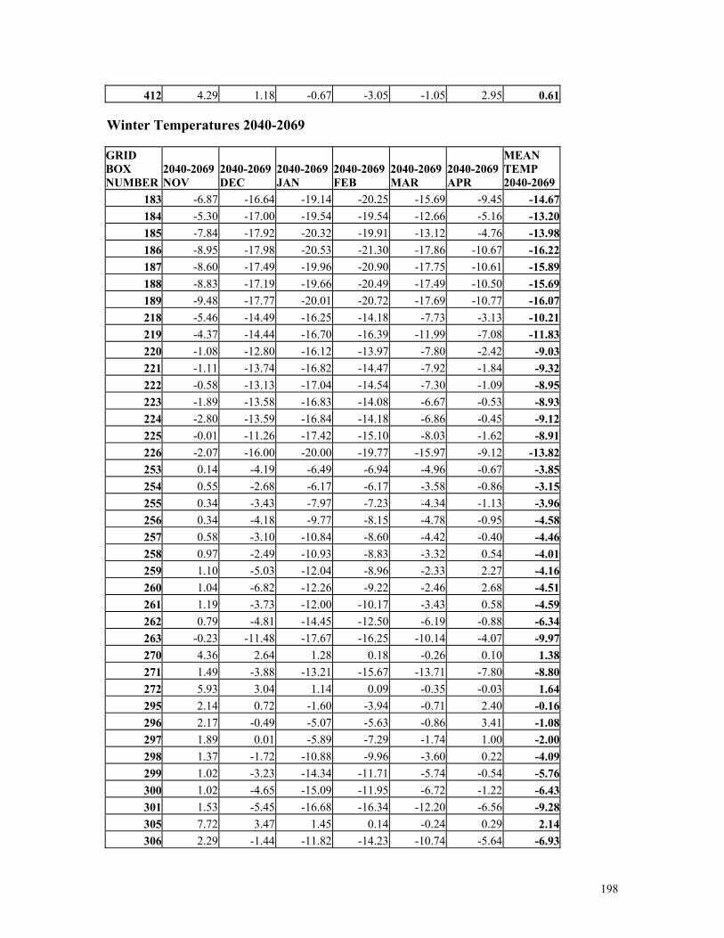
198

412 4.29 1.18 -0.67 -3.05 -1.05 2.95 0.61 Winter Temperatures 2040-2069 GRID BOX NUMBER

2040-2069 NOV

2040-2069 DEC

2040-2069JAN

2040-2069FEB

2040-2069MAR

2040-2069APR

MEAN TEMP 2040-2069

183 -6.87 -16.64 -19.14 -20.25 -15.69 -9.45 -14.67184 -5.30 -17.00 -19.54 -19.54 -12.66 -5.16 -13.20185 -7.84 -17.92 -20.32 -19.91 -13.12 -4.76 -13.98186 -8.95 -17.98 -20.53 -21.30 -17.86 -10.67 -16.22187 -8.60 -17.49 -19.96 -20.90 -17.75 -10.61 -15.89188 -8.83 -17.19 -19.66 -20.49 -17.49 -10.50 -15.69189 -9.48 -17.77 -20.01 -20.72 -17.69 -10.77 -16.07218 -5.46 -14.49 -16.25 -14.18 -7.73 -3.13 -10.21219 -4.37 -14.44 -16.70 -16.39 -11.99 -7.08 -11.83220 -1.08 -12.80 -16.12 -13.97 -7.80 -2.42 -9.03221 -1.11 -13.74 -16.82 -14.47 -7.92 -1.84 -9.32222 -0.58 -13.13 -17.04 -14.54 -7.30 -1.09 -8.95223 -1.89 -13.58 -16.83 -14.08 -6.67 -0.53 -8.93224 -2.80 -13.59 -16.84 -14.18 -6.86 -0.45 -9.12225 -0.01 -11.26 -17.42 -15.10 -8.03 -1.62 -8.91226 -2.07 -16.00 -20.00 -19.77 -15.97 -9.12 -13.82253 0.14 -4.19 -6.49 -6.94 -4.96 -0.67 -3.85254 0.55 -2.68 -6.17 -6.17 -3.58 -0.86 -3.15255 0.34 -3.43 -7.97 -7.23 -4.34 -1.13 -3.96256 0.34 -4.18 -9.77 -8.15 -4.78 -0.95 -4.58257 0.58 -3.10 -10.84 -8.60 -4.42 -0.40 -4.46258 0.97 -2.49 -10.93 -8.83 -3.32 0.54 -4.01259 1.10 -5.03 -12.04 -8.96 -2.33 2.27 -4.16260 1.04 -6.82 -12.26 -9.22 -2.46 2.68 -4.51261 1.19 -3.73 -12.00 -10.17 -3.43 0.58 -4.59262 0.79 -4.81 -14.45 -12.50 -6.19 -0.88 -6.34263 -0.23 -11.48 -17.67 -16.25 -10.14 -4.07 -9.97270 4.36 2.64 1.28 0.18 -0.26 0.10 1.38271 1.49 -3.88 -13.21 -15.67 -13.71 -7.80 -8.80272 5.93 3.04 1.14 0.09 -0.35 -0.03 1.64295 2.14 0.72 -1.60 -3.94 -0.71 2.40 -0.16296 2.17 -0.49 -5.07 -5.63 -0.86 3.41 -1.08297 1.89 0.01 -5.89 -7.29 -1.74 1.00 -2.00298 1.37 -1.72 -10.88 -9.96 -3.60 0.22 -4.09299 1.02 -3.23 -14.34 -11.71 -5.74 -0.54 -5.76300 1.02 -4.65 -15.09 -11.95 -6.72 -1.22 -6.43301 1.53 -5.45 -16.68 -16.34 -12.20 -6.56 -9.28305 7.72 3.47 1.45 0.14 -0.24 0.29 2.14306 2.29 -1.44 -11.82 -14.23 -10.74 -5.64 -6.93

199

307 1.54 -2.67 -10.95 -11.43 -8.11 -4.28 -5.98308 1.23 -2.85 -10.57 -11.13 -7.81 -3.97 -5.85309 1.34 -1.93 -11.03 -13.40 -10.39 -5.48 -6.81335 2.45 -3.19 -9.82 -7.00 -1.42 4.20 -2.46336 2.47 -1.54 -9.94 -7.83 -2.73 1.81 -2.96337 2.93 -0.68 -11.93 -13.10 -8.93 -2.57 -5.71338 3.28 -1.05 -12.08 -13.00 -9.02 -3.36 -5.87339 3.38 -0.38 -11.53 -13.03 -9.40 -4.39 -5.89340 2.87 0.08 -7.42 -8.38 -5.29 -0.69 -3.14341 1.86 -1.25 -9.23 -9.60 -6.49 -2.17 -4.48342 1.08 -3.25 -10.38 -10.62 -7.07 -2.81 -5.51343 1.14 -2.21 -9.94 -10.47 -6.82 -2.49 -5.13371 4.12 -0.32 -5.80 -4.59 -0.11 5.71 -0.17372 3.87 -0.02 -6.15 -5.28 -1.18 3.25 -0.92373 4.11 0.34 -5.17 -5.30 -1.55 2.45 -0.85374 4.30 0.57 -4.41 -5.32 -1.68 2.92 -0.61375 4.19 0.58 -3.42 -5.61 -2.22 2.00 -0.75376 3.57 0.43 -3.54 -6.15 -3.25 0.64 -1.38377 2.90 0.20 -4.66 -6.75 -3.61 0.55 -1.90378 3.47 0.69 -3.48 -5.92 -2.87 0.99 -1.19379 8.61 5.15 2.12 0.79 0.74 2.16 3.26411 5.53 1.43 -0.12 -1.14 0.17 5.77 1.94412 5.58 1.63 0.12 -0.91 0.42 5.83 2.11

Winter Temperatures 2070-2099 GRID BOX NUMBER

2070-2099 NOV

2070-2099 DEC

2070-2099JAN

2070-2099FEB

2070-2099MAR

2070-2099APR

MEAN TEMP 2070-2099

183 -0.76 -11.74 -16.09 -15.61 -12.36 -6.51 -10.51184 -0.43 -11.68 -16.53 -14.70 -8.64 -1.45 -8.90185 -2.66 -14.06 -16.70 -14.94 -8.63 -0.69 -9.61186 -4.42 -15.32 -16.88 -16.23 -13.79 -6.19 -12.14187 -4.24 -15.32 -16.80 -16.09 -14.01 -5.71 -12.03188 -3.96 -14.55 -16.72 -16.07 -14.31 -6.11 -11.95189 -3.77 -14.30 -17.26 -16.71 -14.66 -7.08 -12.30218 -1.26 -9.88 -12.73 -11.32 -5.57 -1.37 -7.02219 -1.04 -10.36 -13.24 -13.76 -9.24 -4.88 -8.75220 0.07 -7.25 -12.98 -11.42 -5.53 -0.81 -6.32221 -0.10 -9.02 -14.13 -11.87 -5.42 -0.35 -6.82222 0.23 -7.60 -14.98 -12.21 -5.12 0.15 -6.59223 -0.30 -8.81 -15.36 -11.93 -4.35 0.86 -6.65224 -0.38 -8.66 -15.10 -11.69 -4.23 1.01 -6.51225 0.77 -2.97 -14.63 -12.18 -5.27 0.02 -5.71226 0.42 -8.15 -16.31 -16.07 -12.11 -5.58 -9.63253 1.83 -0.53 -2.74 -3.19 -0.77 2.46 -0.49

200

254 1.40 0.05 -2.49 -3.58 -1.16 0.53 -0.88255 0.77 -0.45 -4.31 -5.37 -1.95 0.13 -1.86256 0.64 -1.13 -6.13 -6.50 -2.27 0.12 -2.54257 0.91 -0.35 -6.40 -7.04 -1.96 0.49 -2.39258 1.36 0.22 -6.14 -7.46 -1.55 1.69 -1.98259 1.67 -0.68 -7.97 -7.55 -0.88 3.77 -1.94260 1.79 -1.65 -8.76 -7.20 -0.69 4.44 -2.01261 1.71 0.55 -5.98 -7.61 -1.41 1.36 -1.90262 1.27 -0.18 -8.15 -9.47 -3.32 0.32 -3.25263 0.87 -5.25 -13.13 -12.56 -6.36 -1.09 -6.25270 6.45 4.64 3.37 2.45 2.07 2.36 3.56271 2.59 -0.02 -7.94 -11.16 -5.72 -1.37 -3.94272 7.97 5.01 3.23 2.28 1.87 2.21 3.76295 3.12 1.00 0.48 -1.66 0.31 4.35 1.27296 3.10 0.97 -1.43 -3.53 0.06 5.46 0.77297 2.73 0.85 -0.75 -4.88 -0.54 1.90 -0.12298 2.06 0.55 -4.81 -8.17 -1.82 1.00 -1.87299 1.65 0.02 -8.69 -10.19 -3.16 0.50 -3.31300 1.66 -0.26 -10.20 -10.44 -3.89 0.37 -3.80301 2.42 -0.54 -11.61 -14.01 -9.16 -3.62 -6.09305 9.63 5.29 3.51 2.23 1.90 2.50 4.18306 3.77 0.49 -6.04 -9.59 -5.49 -1.11 -2.99307 2.81 0.08 -6.87 -7.88 -4.28 -0.09 -2.71308 2.36 0.05 -6.79 -7.83 -4.14 -0.05 -2.73309 2.32 0.20 -6.34 -9.19 -5.45 -0.79 -3.21335 4.06 -0.83 -5.81 -5.09 0.32 7.29 -0.01336 3.92 -0.13 -4.75 -5.21 -0.54 5.47 -0.21337 4.40 0.66 -4.02 -9.48 -4.50 1.85 -1.85338 4.85 0.68 -4.52 -9.82 -4.99 2.12 -1.95339 5.03 0.86 -4.66 -10.15 -5.62 1.04 -2.25340 4.55 0.79 -2.43 -5.82 -2.13 1.57 -0.58341 3.42 0.34 -5.53 -7.45 -3.99 0.12 -2.18342 2.36 -0.88 -7.45 -8.47 -4.76 -0.60 -3.30343 2.28 -0.17 -6.79 -8.26 -4.43 -0.45 -2.97371 6.07 0.99 -1.97 -2.71 2.02 9.34 2.29372 5.79 1.15 -1.82 -3.17 0.64 7.58 1.69373 6.08 1.36 -0.90 -2.90 0.28 6.80 1.79374 6.21 1.47 -0.74 -2.66 0.29 7.01 1.93375 5.96 1.40 -0.57 -2.92 -0.26 5.89 1.58376 5.19 1.04 -0.92 -3.81 -1.12 3.65 0.67377 4.45 0.76 -1.56 -4.81 -1.32 3.18 0.12378 4.90 1.15 -0.76 -3.75 -0.80 3.51 0.71379 10.10 6.40 3.53 2.25 2.33 3.73 4.72411 7.36 2.67 0.74 0.40 2.80 9.69 3.94412 7.15 2.72 0.93 0.58 2.96 9.55 3.98

201

Appendix 4.6.3: Projected Changes in Snowfall for all Grid Boxes to 2100

GRID BOX NUMBER

1961-1990 mm of water

%CHANGE FROM BASE

2010-2039 mm of water

%CHANGE FROM BASE

2040-2069 mm of water

%CHANGE FROM BASE

2070-2099 mm of water

1 293.41 12.24 329.32 -47.04 155.38 -88.85 32.72 2 294.21 11.41 327.77 -35.51 189.73 -88.61 33.52 3 294.66 11.43 328.35 -35.06 191.35 -88.33 34.38 4 294.83 10.86 326.83 -34.54 192.99 -88.04 35.26 5 294.56 10.54 325.61 -33.99 194.43 -87.75 36.10 6 293.96 10.35 324.39 -21.73 230.09 -87.48 36.79 7 338.71 -4.67 322.88 -31.93 230.56 -88.97 37.37 8 337.12 -4.57 321.70 -31.65 230.44 -88.80 37.75 9 334.91 -4.39 320.19 -31.43 229.64 -88.68 37.92

10 332.14 -3.96 318.99 -31.23 228.42 -88.60 37.87 11 328.94 -3.67 316.86 -31.05 226.80 -88.56 37.62 12 325.54 -3.22 315.05 -31.00 224.63 -88.58 37.19 13 322.03 -2.83 312.92 -31.11 221.84 -88.62 36.63 14 318.58 -2.16 311.69 -31.38 218.62 -88.71 35.97 15 315.43 -1.97 309.23 -31.79 215.14 -88.83 35.22 16 312.53 -1.94 306.46 -32.28 211.66 -88.96 34.51 17 309.94 -1.72 304.61 -32.65 208.74 -89.06 33.91 18 307.67 -1.61 302.72 -32.84 206.63 -89.14 33.40 19 306.05 -1.91 300.22 -42.59 175.71 -89.23 32.95 20 285.04 -6.23 267.30 -38.63 174.92 -88.58 32.54 21 285.25 -6.52 266.65 -38.85 174.42 -76.66 66.58 22 285.67 -16.88 237.44 -39.08 174.03 -76.73 66.49 23 286.20 -17.05 237.41 -39.23 173.93 -76.79 66.42 24 286.82 -16.71 238.90 -39.23 174.29 -76.84 66.43 25 287.78 -16.37 240.68 -39.19 175.00 -76.90 66.47 26 289.18 -16.15 242.49 -39.19 175.86 -76.98 66.56 27 290.93 -16.24 243.69 -39.21 176.86 -77.03 66.81 28 292.83 -16.16 245.50 -39.29 177.79 -77.10 67.06 29 294.71 -16.49 246.12 -39.31 178.85 -77.14 67.38 30 296.63 -16.83 246.71 -39.40 179.75 -77.21 67.62 31 298.73 -17.31 247.03 -39.55 180.58 -77.31 67.78 32 301.07 -17.95 247.04 -39.78 181.29 -77.46 67.86 33 303.50 -18.70 246.74 -40.03 182.02 -77.69 67.72 34 305.60 -19.25 246.76 -49.40 154.64 -89.70 31.48 35 307.23 -19.88 246.15 -49.32 155.70 -89.97 30.81 36 397.51 -4.93 377.91 -48.98 202.80 -92.32 30.51 37 398.65 -4.36 381.25 -48.88 203.81 -92.37 30.44 38 399.21 -3.66 384.60 -48.54 205.45 -92.43 30.22 39 400.30 -3.00 388.29 -48.25 207.17 -92.46 30.16

202

40 401.33 -2.79 390.15 -48.14 208.13 -92.41 30.47 41 400.88 -2.67 390.18 -47.99 208.50 -92.17 31.40 42 398.37 -2.51 388.39 -38.16 246.34 -91.84 32.52 43 394.36 -15.26 334.17 -37.40 246.88 -91.57 33.25 44 389.92 -0.70 387.19 -36.96 245.81 -91.40 33.54 45 386.57 0.08 386.87 -36.88 244.01 -91.35 33.43 46 383.90 0.37 385.31 -36.93 242.12 -91.40 33.00 47 381.30 0.50 383.21 -37.12 239.76 -91.48 32.47 48 378.53 0.68 381.12 -37.70 235.84 -81.75 69.10 49 375.69 1.07 379.70 -38.41 231.37 -81.99 67.64 50 371.26 1.74 377.73 -38.82 227.14 -82.12 66.39 51 366.16 1.78 372.67 -39.11 222.97 -82.12 65.49 52 359.64 1.52 365.11 -38.90 219.74 -81.93 64.97 53 352.61 1.12 356.57 -38.43 217.09 -81.61 64.83 54 346.15 0.87 349.16 -38.15 214.10 -81.15 65.24 55 340.64 0.58 342.61 -38.56 209.29 -80.59 66.12 56 335.39 0.47 336.98 -39.29 203.62 -80.08 66.80 57 329.43 0.86 332.28 -39.76 198.44 -79.72 66.81 58 322.50 -21.87 251.98 -39.67 194.56 -79.40 66.44 59 316.28 -20.83 250.39 -39.27 192.08 -79.00 66.41 60 312.24 -20.31 248.81 -38.47 192.13 -78.74 66.38 61 221.70 7.77 238.93 -26.54 162.85 16.00 257.18 62 224.31 8.15 242.59 -25.42 167.30 15.25 258.51 63 228.25 8.43 247.48 -23.99 173.50 14.74 261.89 64 324.17 -6.04 304.61 -33.49 215.62 -62.02 123.13 65 333.04 4.90 349.34 -32.66 224.27 -49.40 168.51 66 345.18 4.81 361.77 -32.07 234.49 -48.84 176.58 67 360.73 14.07 411.47 -31.81 245.97 -48.11 187.18 68 380.68 21.37 462.05 -31.87 259.37 -48.00 197.96 69 403.68 12.20 452.92 -31.68 275.79 -47.90 210.32 70 349.82 1.87 356.36 -13.63 302.12 3.68 362.70 71 342.60 -28.34 245.50 -49.74 172.20 -91.21 30.13 72 339.52 -10.83 302.75 -51.06 166.15 -91.27 29.65 73 338.88 -11.04 301.46 -39.76 204.14 -91.39 29.17 74 341.78 -12.37 299.50 -38.18 211.29 -91.55 28.88 75 344.43 -4.46 329.08 -36.38 219.12 -81.36 64.21 76 342.17 -5.97 321.75 -34.38 224.52 -81.26 64.14 77 335.10 8.59 363.89 -32.19 227.24 -81.03 63.56 78 330.15 -3.28 319.31 -30.82 228.41 -80.74 63.60 79 333.94 -5.98 313.98 -31.43 228.99 -80.87 63.90 80 341.50 -9.78 308.11 -33.31 227.74 -81.57 62.94 81 346.56 -11.90 305.32 -35.25 224.40 -82.39 61.03 82 347.41 1.49 352.59 -36.56 220.39 -83.21 58.34 83 342.84 4.33 357.69 -37.17 215.39 -83.36 57.06 84 338.51 6.43 360.27 -38.22 209.15 -83.10 57.19

203

85 336.42 -3.78 323.69 -39.23 204.45 -82.96 57.32 86 339.32 8.47 368.06 -39.93 203.83 -74.19 87.57 87 347.10 -8.33 318.19 -40.16 207.71 -74.15 89.71 88 354.97 -18.25 290.18 -40.04 212.84 -65.40 122.81 89 363.14 -0.21 362.40 -41.13 213.78 -64.72 128.11 90 368.39 1.30 373.18 -42.92 210.27 -63.68 133.81 91 257.17 -9.17 233.58 -2.44 250.88 -24.53 194.07 92 252.75 -8.95 230.13 -2.21 247.16 -22.41 196.12 93 247.26 -9.19 224.55 -2.26 241.67 -3.90 237.63 94 243.21 -9.74 219.53 -2.90 236.16 -3.85 233.84 95 239.08 -10.12 214.90 -3.26 231.30 -2.56 232.95 96 234.40 -10.02 210.91 -3.07 227.20 15.60 270.96 97 230.74 -10.27 207.03 -1.48 227.31 16.59 269.01 98 229.32 -9.79 206.87 0.52 230.51 19.00 272.89 99 229.28 2.18 234.27 2.97 236.09 22.20 280.18

100 279.64 -14.13 240.12 -13.40 242.18 2.38 286.30 101 284.58 4.45 297.26 -1.74 279.64 1.39 288.55 102 290.10 5.96 307.40 -2.65 282.40 -0.90 287.48 103 295.86 9.07 322.69 17.36 347.21 -2.35 288.91 104 366.66 -5.74 345.62 -1.66 360.58 -18.18 300.02 105 384.06 -1.99 376.41 1.14 388.45 -14.35 328.95 106 303.13 -20.91 239.74 -60.19 120.66 -100.00 0.00 107 302.68 -21.19 238.54 -59.28 123.24 -100.00 0.00 108 313.32 -23.78 238.83 -57.70 132.53 -100.00 0.00 109 332.56 -27.19 242.13 -56.70 144.00 -100.00 0.00 110 352.36 -20.30 280.83 -46.42 188.80 -100.00 0.00 111 363.90 -19.01 294.74 -45.21 199.37 -100.00 0.00 112 360.30 -15.04 306.10 -41.64 210.27 -100.00 0.00 113 357.40 -13.50 309.14 -37.71 222.62 -91.46 30.53 114 358.69 -14.24 307.61 -37.69 223.49 -92.51 26.86 115 357.62 -1.11 353.65 -40.44 212.99 -82.82 61.44 116 351.82 -17.80 289.20 -34.91 229.01 -83.10 59.45 117 342.32 -19.04 277.15 -36.15 218.57 -82.74 59.10 118 334.55 -19.00 270.98 -37.98 207.51 -82.77 57.66 119 331.46 -17.87 272.23 -40.13 198.43 -81.77 60.43 120 329.98 -16.65 275.04 -39.92 198.26 -100.00 0.00 121 222.62 0.43 223.58 7.90 240.21 -16.41 186.08 122 342.71 -18.28 280.07 -37.65 213.70 -63.56 124.89 123 358.14 -19.33 288.90 -37.17 225.02 -63.83 129.53 124 380.69 -18.37 310.76 -37.87 236.51 -64.15 136.48 125 420.23 -33.59 279.07 -40.64 249.46 -74.32 107.92 126 324.21 -9.87 292.21 -8.28 297.38 -12.96 282.20 127 324.34 -9.72 292.81 -5.34 307.00 4.62 339.31 128 316.69 -8.87 288.60 -4.29 303.12 -11.38 280.65 129 304.85 -8.69 278.35 -35.50 196.61 -13.04 265.11

204

130 345.93 -26.39 254.63 -47.50 181.61 -72.38 95.55 131 290.20 -18.60 236.21 -50.02 145.03 -100.00 0.00 132 284.76 -19.39 229.53 -48.63 146.27 -100.00 0.00 133 288.36 -18.20 235.88 -46.45 154.41 -100.00 0.00 134 304.99 -1.23 301.24 5.07 320.45 -11.05 271.27 135 404.08 -18.33 329.99 -11.49 357.64 -9.44 365.95 136 474.53 -15.54 400.77 -14.78 404.39 -17.92 389.50 137 527.89 -5.82 497.18 8.96 575.18 -19.41 425.42 138 471.78 -2.86 458.29 9.10 514.74 10.51 521.37 139 403.10 3.01 415.23 12.21 452.31 35.32 545.49 140 367.38 7.40 394.56 12.54 413.45 37.30 504.40 141 308.62 -39.88 185.55 -65.57 106.25 -100.00 0.00 142 357.58 -45.80 193.82 -68.39 113.03 -100.00 0.00 143 368.74 -44.14 205.99 -67.13 121.21 -100.00 0.00 144 477.58 -47.35 251.43 -73.23 127.84 -100.00 0.00 145 427.23 -39.36 259.06 -59.29 173.91 -100.00 0.00 146 441.99 -24.16 335.21 -59.85 177.44 -100.00 0.00 147 545.36 -35.57 351.38 -58.62 225.68 -91.77 44.91 148 541.17 -34.97 351.94 -59.48 219.27 -86.65 72.25 149 511.72 -33.46 340.49 -58.76 211.04 -86.72 67.96 150 483.64 -26.16 357.10 -58.09 202.68 -86.93 63.21 151 428.38 -20.79 339.31 -52.67 202.76 -86.30 58.70 152 365.03 -28.54 260.85 -56.72 157.99 -91.50 31.01 153 364.26 -30.17 254.37 -49.75 183.03 -91.28 31.76 154 303.23 -17.55 250.02 -28.39 217.16 -34.47 198.69 155 304.97 -18.49 248.58 -16.60 254.33 -32.97 204.43 156 295.79 -14.57 252.70 -27.98 213.02 -30.05 206.89 157 279.76 -6.75 260.87 -22.26 217.48 -28.68 199.52 158 273.88 -3.24 265.02 -16.76 227.97 -25.67 203.57 159 428.97 -22.92 330.63 -42.20 247.93 -60.48 169.53 160 315.08 -5.53 297.66 -14.57 269.17 -14.43 269.61 161 350.22 -8.07 321.96 -14.48 299.51 -14.15 300.68 162 373.96 -6.44 349.87 -13.41 323.81 -12.76 326.24 163 376.34 -2.74 366.03 -14.16 323.03 -12.01 331.12 164 358.16 -17.81 294.37 -14.63 305.76 -12.05 315.00 165 329.79 -19.23 266.36 -16.06 276.83 -13.67 284.71 166 252.78 -8.55 231.16 -38.44 155.61 -100.00 0.00 167 266.84 -22.48 206.86 -59.51 108.04 -100.00 0.00 168 246.53 -19.49 198.48 -56.78 106.54 -100.00 0.00 169 228.18 -24.10 173.19 -48.16 118.28 -100.00 0.00 170 263.72 -19.85 211.38 -42.17 152.50 -100.00 0.00 171 503.42 -1.81 494.32 6.39 535.58 -0.54 500.70 172 732.31 -1.68 720.04 -9.10 665.68 -15.05 622.12 173 679.94 1.89 692.80 5.16 715.03 12.50 764.91 174 550.07 6.51 585.87 9.48 602.19 21.81 670.05

205

175 461.66 8.32 500.08 13.15 522.36 27.83 590.12 176 301.12 -36.99 189.75 -66.06 102.20 -100.00 0.00 177 296.19 -10.38 265.46 -17.92 243.13 -27.89 213.60 178 319.31 -15.75 269.02 -20.67 253.31 -19.41 257.33 179 346.72 -19.75 278.24 -26.06 256.35 -24.98 260.12 180 365.35 -5.73 344.42 -30.13 255.25 -29.39 257.97 181 361.81 -3.43 349.39 -19.10 292.69 -30.02 253.18 182 344.83 -0.23 344.04 -17.43 284.71 -29.66 242.57 183 321.50 0.56 323.30 -16.04 269.91 -28.33 230.43 184 295.46 -25.68 219.59 -25.58 219.89 -24.16 224.08 185 281.84 -6.64 263.12 -26.86 206.14 -26.97 205.84 186 270.82 3.41 280.06 -25.96 200.51 -26.79 198.28 187 282.52 0.31 283.39 -26.59 207.41 -29.65 198.75 188 312.15 -4.61 297.77 -15.46 263.87 -30.78 216.08 189 339.39 -3.57 327.26 -15.77 285.86 -28.90 241.32 190 342.38 -18.67 278.46 -12.74 298.77 -23.59 261.61 191 361.18 -25.86 267.78 -19.60 290.38 -26.06 267.06 192 329.93 -26.83 241.42 -19.80 264.60 -25.31 246.43 193 306.09 -28.54 218.72 -21.35 240.74 -27.72 221.23 194 201.61 7.38 216.50 13.96 229.76 1.00 203.63 195 274.89 -16.92 228.37 -12.00 241.89 -26.64 201.67 196 318.82 -20.71 252.78 -15.17 270.45 -30.99 220.03 197 405.99 -31.49 278.13 -26.76 297.33 -24.80 305.31 198 421.06 -31.25 289.46 -27.71 304.39 -19.56 338.70 199 408.39 -11.04 363.29 -25.62 303.75 -13.36 353.81 200 686.48 -30.33 478.25 -54.42 312.93 -67.85 220.70 201 337.55 -22.67 261.02 -22.90 260.26 -12.10 296.71 202 209.55 7.50 225.27 12.67 236.10 -17.32 173.25 203 192.78 3.85 200.20 -5.88 181.44 6.78 205.84 204 181.88 -8.50 166.41 -51.30 88.58 -100.00 0.00 205 206.96 -6.80 192.89 -51.54 100.29 -100.00 0.00 206 268.64 -4.93 255.39 -54.28 122.82 -100.00 0.00 207 517.40 6.06 548.78 2.04 527.98 -36.82 326.88 208 746.19 -5.37 706.14 -10.53 667.63 0.78 752.00 209 840.99 9.88 924.06 13.01 950.42 27.43 1071.70 210 874.14 6.62 931.99 10.13 962.71 18.91 1039.47 211 252.48 -10.09 227.01 -46.78 134.36 -100.00 0.00 212 289.96 -8.68 264.78 -1.74 284.90 -33.18 193.76 213 338.59 -16.73 281.96 -13.43 293.12 -23.86 257.81 214 380.16 -19.68 305.35 -17.50 313.65 -27.06 277.29 215 416.38 -21.11 328.48 -19.64 334.60 -27.38 302.38 216 532.11 -16.58 443.89 -31.75 363.19 -26.45 391.36 217 543.34 -33.88 359.28 -30.89 375.49 -25.98 402.19 218 523.28 -31.84 356.66 -30.09 365.80 -23.22 401.76 219 470.00 -16.47 392.59 -11.08 417.91 -21.01 371.25

206

220 319.48 -3.79 307.38 -1.87 313.52 -22.87 246.42 221 243.36 11.61 271.62 12.66 274.18 9.10 265.51 222 237.54 1.72 241.62 1.45 240.98 -37.28 149.00 223 243.12 -6.71 226.81 -6.41 227.53 -25.67 180.72 224 248.51 -8.10 228.39 -4.79 236.60 -22.35 192.97 225 261.53 -6.93 243.40 -4.43 249.96 -35.31 169.18 226 308.86 0.75 311.17 -14.25 264.85 -26.53 226.93 227 305.27 3.55 316.12 7.20 327.26 -25.21 228.31 228 286.62 4.18 298.60 11.45 319.44 -22.31 222.66 229 270.51 3.54 280.10 6.56 288.24 -23.92 205.81 230 280.00 -0.67 278.13 -2.18 273.89 -32.67 188.52 231 300.31 -1.30 296.41 -7.33 278.29 -36.91 189.45 232 330.60 -7.10 307.13 -9.75 298.37 -35.60 212.90 233 340.52 -7.64 314.49 -5.37 322.23 -30.59 236.36 234 669.75 -40.70 397.18 -64.84 235.49 -79.21 139.21 235 473.76 -23.17 363.98 -48.77 242.69 -69.58 144.10 236 376.63 -6.28 352.98 -7.71 347.61 -15.78 317.21 237 358.91 -12.37 314.50 -11.09 319.11 -38.83 219.55 238 289.98 -4.85 275.91 -19.45 233.57 -32.58 195.49 239 190.95 -6.28 178.95 -45.73 103.62 -100.00 0.00 240 161.59 19.40 192.93 -31.32 110.98 -100.00 0.00 241 180.86 22.55 221.65 -46.76 96.28 -100.00 0.00 242 504.72 -9.43 457.12 -1.75 495.86 -16.56 421.13 243 651.43 29.41 843.01 13.28 737.92 -15.62 549.69 244 995.04 3.62 1031.03 -8.54 910.06 -32.29 673.74 245 1181.33 1.19 1195.40 -9.62 1067.72 -33.67 783.58 246 310.82 -65.88 106.04 -100.00 0.00 -100.00 0.00 247 335.22 10.57 370.65 -25.54 249.60 -37.99 207.87 248 381.33 -7.58 352.42 -2.60 371.42 -36.74 241.25 249 478.80 -9.58 432.92 -9.18 434.86 -39.21 291.06 250 612.59 5.70 647.53 -35.19 397.02 -42.07 354.86 251 765.14 5.02 803.57 -35.04 497.03 -65.81 261.60 252 1064.60 -13.16 924.49 -22.37 826.47 -55.49 473.86 253 1120.71 -13.29 971.71 -27.76 809.64 -41.54 655.15 254 1027.05 -9.40 930.52 -24.55 774.89 -55.08 461.38 255 826.30 -8.73 754.19 -24.38 624.82 -35.41 533.72 256 549.55 -0.87 544.76 -22.23 427.37 -32.30 372.04 257 384.03 -23.87 292.36 -22.31 298.34 -36.52 243.77 258 280.42 -39.34 170.11 -38.99 171.09 -62.52 105.11 259 198.41 -7.84 182.85 -29.16 140.55 -31.83 135.26 260 191.67 -4.67 182.72 -29.24 135.62 -26.33 141.19 261 258.26 -20.04 206.50 -39.72 155.68 -52.77 121.98 262 308.62 -18.95 250.15 -23.04 237.52 -27.91 222.48 263 391.95 -11.68 346.15 -12.02 344.82 -22.34 304.38 264 384.17 8.78 417.89 -10.29 344.66 -24.99 288.16

207

265 378.20 1.96 385.61 -16.74 314.88 -33.37 251.99 266 356.89 0.71 359.44 -33.70 236.63 -36.08 228.13 267 318.99 -26.02 236.00 -65.11 111.28 -100.00 0.00 268 292.71 -25.92 216.84 -87.12 37.70 -100.00 0.00 269 355.87 -36.37 226.43 -89.26 38.23 -100.00 0.00 270 353.96 -29.67 248.94 -87.83 43.07 -100.00 0.00 271 392.69 -10.57 351.17 -8.39 359.73 -24.80 295.30 272 444.85 -31.56 304.44 -77.18 101.54 -100.00 0.00 273 364.13 -20.58 289.21 -74.04 94.51 -100.00 0.00 274 231.67 -32.74 155.83 -79.31 47.92 -100.00 0.00 275 0.00 0.00 94.15 0.00 0.00 0.00 0.00 276 0.00 0.00 186.89 0.00 217.97 0.00 0.00 277 0.00 0.00 76.50 0.00 0.00 0.00 0.00 278 739.08 5.66 780.89 -13.42 639.93 -24.27 559.70 279 867.77 4.65 908.11 5.70 917.20 -18.25 709.38 280 661.70 -20.17 528.22 -64.00 238.20 -9.04 601.89 281 187.63 -100.00 0.00 -100.00 0.00 -100.00 0.00 282 292.45 -100.00 0.00 -100.00 0.00 -100.00 0.00 283 229.48 -100.00 0.00 -100.00 0.00 -100.00 0.00 284 438.52 -51.71 211.75 -100.00 0.00 -100.00 0.00 285 0.00 0.00 0.00 0.00 0.00 0.00 0.00 286 0.00 0.00 0.00 0.00 0.00 0.00 0.00 287 0.00 0.00 0.00 0.00 0.00 0.00 0.00 288 0.00 0.00 0.00 0.00 0.00 0.00 0.00 289 0.00 0.00 0.00 0.00 0.00 0.00 0.00 290 838.33 -44.97 461.35 -100.00 0.00 -100.00 0.00 291 1047.20 -43.50 591.66 -58.98 429.55 -100.00 0.00 292 730.33 -1.14 722.00 -39.95 438.54 -83.64 119.51 293 440.81 -11.44 390.37 -12.22 386.96 -46.02 237.95 294 300.23 -13.70 259.11 -40.41 178.91 -61.43 115.80 295 188.50 7.41 202.46 -27.45 136.75 -75.52 46.14 296 177.02 6.38 188.32 4.86 185.63 -45.67 96.18 297 218.37 -12.98 190.02 -38.35 134.63 -34.45 143.14 298 236.16 -3.11 228.82 -14.95 200.85 -38.26 145.81 299 300.40 -20.57 238.61 -8.42 275.11 -51.50 145.68 300 293.77 -20.62 233.19 -11.23 260.77 -32.25 199.03 301 353.96 -11.68 312.61 -32.31 239.58 -27.46 256.78 302 366.59 -35.87 235.08 -64.13 131.50 -100.00 0.00 303 431.32 -49.26 218.87 -81.05 81.75 -100.00 0.00 304 437.94 -45.60 238.24 -91.25 38.34 -100.00 0.00 305 397.52 -31.07 274.02 -87.70 48.90 -100.00 0.00 306 443.46 -11.22 393.71 -23.71 338.33 -39.53 268.17 307 507.16 -10.88 451.98 -25.88 375.92 -39.41 307.31 308 504.75 -11.37 447.37 -27.35 366.69 -39.78 303.95 309 417.98 4.65 437.43 -17.64 344.26 -32.04 284.05

208

310 118.24 116.60 256.10 69.50 200.41 -100.00 0.00 311 0.00 0.00 223.58 0.00 244.59 0.00 182.73 312 0.00 0.00 247.77 0.00 197.74 0.00 0.00 313 0.00 0.00 183.82 0.00 111.50 0.00 0.00 314 0.00 0.00 0.00 0.00 204.18 0.00 199.87 315 0.00 0.00 0.00 0.00 0.00 0.00 0.00 316 0.00 0.00 0.00 0.00 0.00 0.00 0.00 317 0.00 0.00 0.00 0.00 0.00 0.00 0.00 318 0.00 0.00 0.00 0.00 0.00 0.00 0.00 319 0.00 0.00 0.00 0.00 0.00 0.00 0.00 320 0.00 0.00 0.00 0.00 0.00 0.00 0.00 321 0.00 0.00 0.00 0.00 0.00 0.00 0.00 322 0.00 0.00 0.00 0.00 0.00 0.00 0.00 323 0.00 0.00 0.00 0.00 0.00 0.00 0.00 324 0.00 0.00 0.00 0.00 0.00 0.00 0.00 325 0.00 0.00 0.00 0.00 0.00 0.00 0.00 326 0.00 0.00 0.00 0.00 0.00 0.00 0.00 327 0.00 0.00 0.00 0.00 0.00 0.00 0.00 328 707.80 -38.66 434.14 -100.00 0.00 -100.00 0.00 329 771.82 -12.62 674.40 -55.98 339.77 -83.25 129.25 330 445.33 -14.72 379.79 -34.39 292.16 -81.24 83.53 331 283.22 -16.30 237.07 -36.62 179.51 -79.16 59.03 332 217.70 -17.21 180.23 -41.53 127.29 -57.94 91.57 333 152.43 2.59 156.37 -19.41 122.83 -51.11 74.51 334 147.44 6.48 156.99 12.44 165.79 -50.52 72.96 335 160.11 5.49 168.90 8.07 173.02 -12.36 140.32 336 233.42 -16.66 194.53 -20.22 186.23 -10.25 209.50 337 254.48 9.98 279.88 3.28 262.83 -32.53 171.69 338 360.49 -18.63 293.34 -22.93 277.82 -53.01 169.37 339 394.20 -18.91 319.65 -19.87 315.87 -54.36 179.90 340 369.28 -1.16 364.99 -20.18 294.76 -40.97 217.98 341 414.98 -0.30 413.72 8.04 448.35 -39.12 252.64 342 632.46 -31.26 434.73 -23.26 485.34 -23.87 481.46 343 520.77 -19.08 421.39 -7.85 479.91 -8.62 475.87 344 407.17 6.52 433.72 14.97 468.13 -32.45 275.06 345 436.29 4.82 457.30 -41.67 254.49 -37.05 274.65 346 0.00 0.00 179.79 0.00 0.00 0.00 0.00 347 0.00 0.00 181.11 0.00 191.85 0.00 0.00 348 0.00 0.00 0.00 0.00 0.00 0.00 0.00 349 0.00 0.00 0.00 0.00 0.00 0.00 0.00 350 0.00 0.00 0.00 0.00 0.00 0.00 0.00 351 0.00 0.00 0.00 0.00 0.00 0.00 0.00 352 0.00 0.00 0.00 0.00 0.00 0.00 0.00 353 0.00 0.00 0.00 0.00 0.00 0.00 0.00 354 0.00 0.00 0.00 0.00 0.00 0.00 0.00

209

355 0.00 0.00 0.00 0.00 0.00 0.00 0.00 356 0.00 0.00 0.00 0.00 0.00 0.00 0.00 357 0.00 0.00 0.00 0.00 0.00 0.00 0.00 358 0.00 0.00 0.00 0.00 0.00 0.00 0.00 359 0.00 0.00 0.00 0.00 0.00 0.00 0.00 360 0.00 0.00 0.00 0.00 0.00 0.00 0.00 361 0.00 0.00 0.00 0.00 0.00 0.00 0.00 362 0.00 0.00 0.00 0.00 0.00 0.00 0.00 363 0.00 0.00 0.00 0.00 0.00 0.00 0.00 364 416.48 -100.00 0.00 -100.00 0.00 -100.00 0.00 365 543.29 -34.18 357.62 -100.00 0.00 -100.00 0.00 366 314.76 -30.71 218.09 -100.00 0.00 -100.00 0.00 367 207.76 -27.49 150.65 -100.00 0.00 -100.00 0.00 368 167.88 -23.72 128.05 -48.21 86.95 -100.00 0.00 369 173.56 -3.71 167.12 -48.52 89.35 -47.84 90.53 370 232.47 -22.60 179.94 -60.02 92.95 -61.08 90.48 371 194.44 0.04 194.52 4.88 203.92 -50.85 95.57 372 201.10 4.48 210.11 4.24 209.62 -47.78 105.02 373 216.52 8.14 234.14 -21.40 170.19 -50.24 107.74 374 255.71 2.37 261.78 -19.67 205.41 -52.77 120.76 375 317.63 -28.36 227.54 -25.19 237.60 -23.67 242.45 376 466.72 -18.97 378.17 -40.39 278.23 -40.04 279.84 377 486.58 5.18 511.78 -38.61 298.72 -37.19 305.60 378 499.73 -16.20 418.77 -38.57 307.00 -38.53 307.17 379 405.04 -49.93 202.79 -100.00 0.00 -100.00 0.00 380 199.14 -100.00 0.00 -100.00 0.00 -100.00 0.00 381 307.36 -29.75 215.91 -100.00 0.00 -100.00 0.00 382 0.00 0.00 0.00 0.00 0.00 0.00 0.00 383 0.00 0.00 0.00 0.00 0.00 0.00 0.00 384 0.00 0.00 0.00 0.00 0.00 0.00 0.00 385 0.00 0.00 0.00 0.00 0.00 0.00 0.00 386 0.00 0.00 0.00 0.00 0.00 0.00 0.00 387 0.00 0.00 0.00 0.00 0.00 0.00 0.00 388 0.00 0.00 0.00 0.00 0.00 0.00 0.00 389 0.00 0.00 0.00 0.00 0.00 0.00 0.00 390 0.00 0.00 0.00 0.00 0.00 0.00 0.00 391 0.00 0.00 0.00 0.00 0.00 0.00 0.00 392 0.00 0.00 0.00 0.00 0.00 0.00 0.00 393 0.00 0.00 0.00 0.00 0.00 0.00 0.00 394 0.00 0.00 0.00 0.00 0.00 0.00 0.00 395 0.00 0.00 0.00 0.00 0.00 0.00 0.00 396 0.00 0.00 0.00 0.00 0.00 0.00 0.00 397 0.00 0.00 0.00 0.00 0.00 0.00 0.00 398 0.00 0.00 0.00 0.00 0.00 0.00 0.00 399 0.00 0.00 0.00 0.00 0.00 0.00 0.00

210

400 384.20 -100.00 0.00 -100.00 0.00 -100.00 0.00 401 368.98 -47.63 193.23 -100.00 0.00 -100.00 0.00 402 278.90 -24.45 210.70 -100.00 0.00 -100.00 0.00 403 215.08 -27.43 156.09 -100.00 0.00 -100.00 0.00 404 178.21 -28.35 127.68 -100.00 0.00 -100.00 0.00 405 150.80 -20.91 119.27 -42.57 86.61 -100.00 0.00 406 147.40 -47.72 77.06 -41.18 86.70 -100.00 0.00 407 173.99 -16.27 145.69 -41.49 101.81 -100.00 0.00 408 157.41 3.88 163.52 -26.30 116.01 -100.00 0.00 409 183.64 -1.39 181.09 -67.52 59.65 -100.00 0.00 410 226.45 0.15 226.79 -67.63 73.31 -100.00 0.00 411 260.38 1.81 265.10 -35.08 169.03 -100.00 0.00 412 264.14 5.62 278.98 -70.12 78.92 -100.00 0.00 413 273.20 -29.96 191.34 -100.00 0.00 -100.00 0.00 414 0.00 0.00 0.00 0.00 0.00 0.00 0.00 415 0.00 0.00 0.00 0.00 0.00 0.00 0.00 416 0.00 0.00 0.00 0.00 0.00 0.00 0.00 417 0.00 0.00 0.00 0.00 0.00 0.00 0.00 418 0.00 0.00 0.00 0.00 0.00 0.00 0.00 419 0.00 0.00 0.00 0.00 0.00 0.00 0.00 420 0.00 0.00 0.00 0.00 0.00 0.00 0.00 421 0.00 0.00 0.00 0.00 0.00 0.00 0.00 422 0.00 0.00 0.00 0.00 0.00 0.00 0.00 423 0.00 0.00 0.00 0.00 0.00 0.00 0.00 424 0.00 0.00 0.00 0.00 0.00 0.00 0.00 425 0.00 0.00 0.00 0.00 0.00 0.00 0.00 426 0.00 0.00 0.00 0.00 0.00 0.00 0.00 427 0.00 0.00 0.00 0.00 0.00 0.00 0.00 428 0.00 0.00 0.00 0.00 0.00 0.00 0.00 429 0.00 0.00 0.00 0.00 0.00 0.00 0.00 430 0.00 0.00 0.00 0.00 0.00 0.00 0.00 431 0.00 0.00 0.00 0.00 0.00 0.00 0.00 432 0.00 0.00 0.00 0.00 0.00 0.00 0.00 433 0.00 0.00 0.00 0.00 0.00 0.00 0.00 434 0.00 0.00 0.00 0.00 0.00 0.00 0.00 435 535.56 -44.80 295.63 -100.00 0.00 -100.00 0.00 436 488.67 -10.88 435.51 -49.75 245.55 -100.00 0.00 437 364.60 -14.11 313.17 -56.93 157.03 -100.00 0.00 438 196.68 9.31 215.00 -73.06 52.99 -100.00 0.00 439 150.32 -57.90 63.29 -100.00 0.00 -100.00 0.00 440 57.25 -54.51 26.04 -100.00 0.00 -100.00 0.00 441 66.60 -58.57 27.59 -100.00 0.00 -100.00 0.00 442 90.41 -100.00 0.00 -100.00 0.00 -100.00 0.00 443 120.66 -8.72 110.14 -100.00 0.00 -100.00 0.00 444 227.60 -41.10 134.05 -100.00 0.00 -100.00 0.00

211

445 318.17 -51.56 154.11 -76.32 75.33 -100.00 0.00 446 273.79 -34.12 180.37 -100.00 0.00 -100.00 0.00 447 95.72 -100.00 0.00 -100.00 0.00 -100.00 0.00 448 0.00 0.00 0.00 0.00 0.00 0.00 0.00 449 0.00 0.00 0.00 0.00 0.00 0.00 0.00 450 0.00 0.00 0.00 0.00 0.00 0.00 0.00 451 0.00 0.00 0.00 0.00 0.00 0.00 0.00 452 0.00 0.00 0.00 0.00 0.00 0.00 0.00 453 0.00 0.00 0.00 0.00 0.00 0.00 0.00 454 0.00 0.00 0.00 0.00 0.00 0.00 0.00 455 0.00 0.00 0.00 0.00 0.00 0.00 0.00

212

Chapter 5: Drinking Water Supply and Wastewater Treatment This chapter deals with the main impacts of climate change on water

infrastructure and the required adaptation costs. We suggest that the main impacts of

climate change on water utilities are likely to be on (a) the supply of drinking water, and

(b) the treatment of wastewater, as the level of precipitation changes due to climate

change. Sections 5.1, 5.1.1 and 5.1.2 give the national context of water availability,

including consumption and prices of water in Canada. In Section 5.1.3, we provide an

introduction to the impact of climate change on water resources. In Section 5.1.4, we

outline some of the potential adaptations to municipal water infrastructure. This is

followed by detailed case studies of water utilities in the different ecoclimatic zones of

Canada. Section 5.2 is a case study of Toronto, for which the adaptation costs are

considered in some detail. The remaining case studies are organized as follows: Section

5.3, The Region of Niagara; Section 5.4, Montréal; Section 5.5, Halifax; 5.6.1, Regina;

5.7, Humboldt; 5.8, Swift Current; 5.9, Lethbridge; 5.10, Prince George; 5.11, Penticton;

5.12, Yellowknife; 5.13, Norman Wells; and 5.14, Directions for Future Research.

5.1: Water in Canada: An Introduction

Canada is rich in natural resources, including water. The world’s oceans contain

more than 95% of the earth’s water, but this water is too salty to use in its normal state,

except as habitat for marine organisms and a medium for human transportation. The

remaining water, less than 5%, is fresh. One-third of this water is stored in ice caps and

glaciers, and most of the rest is groundwater, with only a very small portion, about 0.2%

found in the soil and in surface waters, such as lakes and rivers.

According to Environment Canada, Canada probably has more lake area than any

other country in the world. It shares with the United States the Great Lakes, which hold

213

about 18% of the world’s entire surface freshwater. On average, about 9% of the world’s

renewable freshwater supply flows in Canadian rivers. Since Canada occupies 7% of the

earth’s land area, its freshwater supplies are not out of proportion. But with less than 1%

of the world’s population, Canada is generously supplied with freshwater, though this

supply is not evenly distributed throughout the country.

Because of Canada’s different climatic zones, some parts of British Columbia and

the Prairies are so dry that they compare with northern Mexico and much of Australia.

Other parts of Canada, such as southern Ontario, suffer water shortages only during

extended dry periods. In these regions the climate is more like the mid-western United

States and central Europe. Canada’s east and west coasts receive a good deal of rain,

comparing more to Scandinavia. Thus, water management in Canada must be adapted to

a wide range of conditions and can benefit from experience obtained in other parts of the

world.

We can think of two basic ways in which we use water:

1. Instream uses, such as hydroelectric power generation, transportation, fisheries,

wildlife, recreation, and waste disposal, take place with the water remaining in its

natural setting, "in the stream.”

2. Withdrawal uses, such as thermal power generation, mineral extraction, irrigation,

manufacturing, and municipal use. This use removes water from its natural setting

for a period of time and for a particular use, and eventually returns all or part of it

to the source. The difference between the amount of water withdrawn and the

amount of water returned to the source is water "consumed" (for example, by

evaporating and not returning to the local source).

214

Much of the land producing fruits and vegetables, as well as a significant amount of

the land used to grow tobacco, is irrigated. In western Canada, irrigated forage crops

sustain the livestock industry. According to the 1996 census, there were 21 448 farms in

Canada reporting that they used irrigation on a total of 856 132 hectares of farmland. The

provincial breakdown is as follows:

Alberta, 516 600 hectares British Columbia, 115 374 hectares Saskatchewan, 97 378 hectares Ontario, 66 090 hectares Quebec, 33 611 hectares Manitoba, 22 190 hectares Atlantic provinces, 4 889 hectares

Across Canada, 12% of the water used in Canadian municipalities comes from

groundwater; the rest is from lakes and rivers. In cities, water is distributed through a

series of pipes connected to a municipal water supply system. In rural areas, it is usually

obtained from wells. Water supply systems typically have intake, treatment, storage, and

distribution components. There are many different treatment types, depending on the

characteristics of the source water. Likewise, the storage and distribution systems vary

greatly between municipalities, depending on the unique characteristics of each city or

town. Rural residents usually have individual groundwater supplies from wells.

Trucks in several regions of Canada deliver water. In the Far North, water may

have to be trucked to homes that do not have conventional water supplies because the

ground is frozen. Water is also delivered by truck in some rural areas of the east and in

the Prairies where wells are shallow and unreliable year round.

Where there are piped systems in the North, the pipes are often buried very deep,

up to 3 or 4 metres, to get below the worst of the frost, and are insulated to prevent the

water from freezing. In permafrost areas, the heat lost from even insulated underground

215

pipes would melt the permafrost and cause the ground to cave in. Therefore, above-

ground utilidors (insulated boxes) are used to carry water, sewer, and sometimes hot

water (for heating) pipes to individual residences. These are heated, insulated, metal or

wood-clad enclosures that are generally installed on piles or blocking.

5.1.1: The Cost of Water in Canada

Water prices across Canada are generally low compared to other countries. The

average household pays $27.65 per month, and uses about 30 000 litres per month, for

water delivered to the residence. Monthly bills range between $15 and $90, the lowest

being in Quebec, Newfoundland, and British Columbia and the highest in the Prairie

Provinces and northern Canada.

Although the operating costs for trucked service are very high, the lower capital

costs make it more economic than piped service for most northern communities.

Consumption is much lower for areas with trucked service, about 200 litres per capita per

day in the Northwest Territories and Nunavut. Several studies show that water revenues

are not sufficient to cover operational, repair, upgrading, or expansion costs. They cover

only a small part of the costs of supplying water. For example, irrigation water charges

recover only about 10% of the development cost of the resource.

The cost of maintaining (repairing and upgrading) municipal water supply and

sewage systems is estimated at $23 billion over the next 10 years in Canada as a whole.

According to the Canadian Water and Wastewater Association there is an investment

shortfall of $16.5 billion in water facilities (mains, storage tanks and treatment plants)

and $36.8 billion in wastewater facilities (sewers, combined sewer and separations and

treatment plants) (Source: Federation of Canadian Municipalities, Quality of Life

Proposal). Over 1.5 million Canadians live in communities with no wastewater

216

treatment, and almost five million live where only primary treatment is available.

Investment in water infrastructure to meet the current climate requirements includes the

Quality of Life Infrastructure Program, a combined Federal/Provincial/Municipal

program. Capital investment in water systems will be $16.5 billion over 10 years, with

$36.8 billion going to wastewater systems.

In Canada, the value of drinking water and wastewater utility assets is

approximately $110 billion. On the assumption of a 40-year life of the infrastructure,

each year a 2.5% replacement should occur. In Canada, close to a billion dollars a year is

spent in the water resources sector on adapting to current climate conditions. Climate

change will most likely increase these expenditures. The existing water supply

infrastructure is aging; pipelines are corroded, clogged and requiring repairs. These old

lines can be replaced with vinyl pipe and fittings, since they are immune to damage from

corrosive soils, and perform better in the cold Canadian climate.

5.1.2: Water Prices in Canada

Provincial and municipal officials set water prices in Canada. Most provinces levy

licence fees to major water users for access to the resource. The provincial licence fees

for water are not set in accordance with any pricing principles, but rather are related to

the cost of administering the licensing program. Municipalities also levy charges to

water users. In many areas, users are charged a flat monthly, quarterly, or annual rate in

exchange for access to unlimited amounts of treated water. In other places, the charges

are based on the volume of water used, as measured by a water meter. Irrigation water

fees are paid according to land area irrigated, not water volume used. Tap water is very

inexpensive compared with some other liquids. For example, 1 litre of water costs about

217

0.001 dollar, while the same amount of bottled water would cost $1.50; cola, $0.85; milk,

$1.10; and table wine, $9.00.

Water rates are a major source of revenue for municipal water utilities.

According to the Federation of Canadian Municipalities, 63% of total water utility

revenue was derived from water rates. The other 27% of revenue came from general

taxes. Many Canadian municipalities charge a flat rate, allowing users unlimited

consumption for a fixed payment. Some municipalities use a declining block structure

that benefits high volume users. This structure also discourages the conservation of water

as well as increasing capacity requirements.

Over 92% of urban households are serviced by municipal water and sewer

systems. All other households, including most of the rural population, are serviced by

private individual systems (usually groundwater), septic tanks and/or tile fields, or

trucked services. In the Northwest Territories and Nunavut, for example, 16% of the

communities have centralized water distribution systems either above or below ground,

while 74% have trucked water supply and waste disposal systems. The remaining 10%

use private systems, water buckets, privies, or trucked services. Specifically, in the

Northwest Territories, seven communities have piped systems: Fort Smith, Hay River,

Yellowknife, and Edzo have inground pipes while Norman Wells, Inuvik, and Rae have

above-ground pipes, or utilidors (insulated boxes). In Nunavut, only Iqaluit, Rankin Inlet,

and Nanisivic have piped aboveground systems.

5.1.3: The Implications of Climate Change for Municipal Water Infrastructure Hydrological changes associated with climate change -- whether it will rain more

or less, for instance -- are more speculative than are temperature projections, especially at

the regional and local geographic scales of interest to water planners. The IPCC suggests

218

that a greenhouse warming will have the following effects on water supplies:

• The timing and regional patterns of precipitation will change, and more intense

precipitation days are likely.

• General circulation models (GCMs) used to predict climate change suggest that a 1.5

to 4.5 degree C rise in global mean temperature would increase global mean

precipitation about 3 to 15 percent. Some of this is due to the conversion of snow

into precipitation.

• Although the regional distribution is uncertain, precipitation is expected to increase in

higher latitudes, particularly in winter. This conclusion extends to the mid-latitudes

in most GCM projections.

• Potential evapotranspiration (FT) -- water evaporated from the surface and transpired

from plants -- rises with air temperature. Consequently, even in areas with increased

precipitation, higher FT rates may lead to reduced runoff; implying a possible

reduction in renewable water supplies.

• More annual runoff caused by increased precipitation is likely in the high latitudes. In

contrast, some lower latitude basins may experience large reductions in runoff and

increased water shortages as a result of a combination of increased evaporation and

decreased precipitation.

• Flood frequencies are likely to increase in many areas, although the amount of

increase for any given climate scenario is uncertain and impacts will vary among

basins. Floods may become less frequent in some areas.

• The frequency and severity of droughts could increase in some areas as a result of a

219

decrease in total rainfall and more frequent dry spells.

• The hydrology of arid land is particularly sensitive to climate variations. Relatively

small changes in temperature and precipitation in these areas could result in large

percentage changes in runoff, increasing the likelihood and severity of droughts

and/or floods.

• Seasonal disruptions might occur in the water supplies of mountainous areas if more

precipitation falls as rain than snow and if the length of the snow storage season is

reduced.

• Water quality problems may increase where there is less flow to dilute contaminants

introduced from natural and human sources.

The implications for municipal water infrastructure under a changed climate are as

follows:

1) Risk of physical system failure. For example, there are key concerns in the Arctic that

climate change will have destructive effects on water and wastewater collection and

distribution systems built on the permafrost base, which is expected to become

increasingly less stable (thaw slump).

2) Contamination due to water-borne disease and/or saltwater intrusion.

3) Seasonal unreliability of supply.

4) Higher demand, but less availability.

There are key concerns about the depletion of groundwater reserves and the

ability of existing reservoirs to capture enough water to satisfy a longer demand season.

In addition, if a greater proportion of rainfall occurs in extreme events, then less water is

available for infiltration and groundwater recharge. In terms of surface water, if snow

220

pack storage is insufficient to fill reservoirs it may necessitate the development of

expanded reservoir capacity and expanded water conservation programs. In the case of

municipalities that draw their water from the Great Lakes, projected falls in lake levels

may necessitate modifications to the collection system.

5.1.4: Potential Adaptations of Municipal Water Infrastructure

New infrastructure may, in some instances, eventually prove to be an appropriate

response to climate induced shifts in hydrological regimes and water demands. But it is

difficult to plan for and justify expensive new projects when the magnitude, timing, and

even the direction of the changes at the basin and regional levels are unknown.

Narrowing the range of uncertainty for improved water planning depends on a better

understanding of (1) the processes governing global and regional climates; (2) the links

between climate and hydrology; (3) the impacts of the climate on unmanaged

ecosystems; (4) the impacts of ecosystem changes on the quantity and quality of water;

and (5) the impacts of increased atmospheric C02 on vegetation and runoff. In the

meantime, the possibility that a warming could result in greater hydrological variability

and storm extremes should be considered in evaluating margins of safety of long-lived

structures such as dams and levees that are under consideration anyway. In particular,

low-cost structural and managerial modifications that ensure against the possibility of a

range of climate-induced impacts are likely to be sought. However, there may well be

instances in which new infrastructure is the only answer and would include:

• Improving levels of wastewater treatment (especially upstream of municipal water

intake) by replacing obsolete wastewater treatment facilities;

• Construction of new reservoirs to increase capacity;

221

• Replacement of freshwater collection systems if changes in water levels make

extraction impossible; and

• Replacement of wastewater treatment plants if changing water levels make plant

operation impossible.

More importantly, the prospect that a global warming will alter in unknown ways

local and regional supplies and demands reinforces the need for institutions that facilitate

adaptation to whatever the future brings and promote more efficient water management

and use. Unlike the structural supply-side approach, demand management that introduces

incentives to conserve and opportunities to reallocate supplies as conditions change does

not require long lead times, large financial commitments, or accurate information about

the future climate. Water demand management measures include metering, leak

detection, water pricing, rational water permitting and recycling measures.

In the rest of this chapter we consider the impact of climate change on drinking

water supply and the wastewater treatment in the major ecoclimatic zones of Canada.

We consider a series of case studies that are representative of the ecoclimatic zones.

5.2: Toronto, ON 5.2.1: Introduction

The City of Toronto’s Water and Wastewater Services Division was created by

the amalgamation of the water and sewer functions from seven former municipalities and

one public utility on January 1, 1998. The division supplies fresh water to over 3 million

residents in Toronto and York region and treats all wastewater from Toronto, a portion of

Peel region and the Greater Toronto Airport Authority (see Figure 5.2.1).

Although the Water and Wastewater Division is presently owned by the City of

Toronto, the division is required to be a financially self-sustaining entity with distinctly

222

separate budgets for each component of its operation. While this budget structure

removes the burden from municipal taxes, it fails to provide an adequate mechanism to

deal with the adaptation to climate change.

Figure 5.2.1: Toronto and Niagara

5.2.2: Great Lake Levels The waters of the Great Lakes are a non-renewable resource, composed of

numerous aquifers that flow into the tributaries of the Great Lakes and fill the lakes

themselves. On average, less than 1% of the waters of the Great Lakes are renewed

G r id B o x 44 5 - T o ron to a n d N ia g ar a

100 0 100 200 Kilometers

N

EW

S

Toronto

N ia gara

223

annually by precipitation, surface water runoff, and inflow from groundwater sources.

The primary source of natural water supply to the Great Lakes is precipitation, and levels

are determined by the combined influence of precipitation, upstream inflows,

groundwater, surface water runoff, evaporation, and diversions into and out of the

system, consumptive use, dredging, and water level regulation. Climatic conditions

control precipitation, runoff, and direct supply to the lakes, as well as the rate of

evaporation, and these are the primary factors in determining water levels. During dry,

hot-weather periods, inflow is decreased and evaporation increased resulting in lower

lake levels and reduced flows.

In the past, the Great Lakes have had a small range in lake levels, approximately

6.5 feet from the recorded monthly maximum to the recorded monthly minimum.

Seasonal cycles can vary from 10 to 12 inches. During the past thirty years, lake levels

have been the highest in recorded history, due to increased summer and fall precipitation.

Recently lake levels have experienced the second largest decline in one hundred years.

Results from computer climate models have been used to explore impacts on water

levels, assuming likely scenarios of future atmospheric greenhouse gas concentrations.

The information from these models has been used to develop climate scenarios that have

been included in hydrologic models. Early impact assessments, based on equilibrium

2XCO2 scenarios, suggest global warming will result in a lowering of water supplies and

lake levels and in a reduction of outflows from the Basin. Some projections show a

lowering of lake levels by up to a meter or more by 2050. (Preparing for Climate

Change, The Potential Consequences of Climate Variability and Change, The Great

Lakes; Great Lakes Regional Assessment Group, 2000).

224

The General Circulation Model, CGCM1, like several other models, has shown an

increase in lake surface temperature, a decrease in basin runoff and an increase in lake

evaporation, resulting in reduced inter-lake channel flow and water levels on all of the

Great Lakes. Mean annual runoff is reduced, and combines with an increase in lake

surface evaporation due to a strong increase in lake surface temperature, to produce a

reduction in net basin supply. Net basin supply is the water input to the lakes by runoff

from its basin plus input from over-lake precipitation minus output to over-lake

evaporation. The CGCM1 shows that lake level reductions from 0.7-2.4 feet are

predicted by 2030. A one meter drop in the levels of Lakes Michigan and Huron in thirty

years would have a severe impact on Lake St. Clair and Lake Erie, whose levels would

drop by about 2 feet. A lake level drop of one meter in Lake Michigan could cause

thousands of municipal water intakes and wells to be moved or extended. In general,

municipal water intakes are located 20 to 40 feet from the water’s edge, resulting in water

supplies of superior quality.

5.2.3: The Water Supply Services Component

Lake Ontario is the only source of fresh water for the city. Water is drawn into

the Toronto system from four filtration plants, which have intake pipes located one to

three kilometres from shore and at a water depth of 15 metres. Once the raw water enters

the system, it is screened, filtered and treated before entering a transmission network.

The network consists of 487 kilometres of 15 centimetres to 250 centimetres in diameter

steel and cast iron water mains. Water pressure is maintained in the network through the

Central Pumping Control Facility. At this facility operators receive pipeline flow,

distribution system pressures, reservoir levels, pumping equipment status and power

demands from 12 separate pressure districts located on six different elevation levels.

225

During 1999, an average of 1,503 mega litres of water was pumped per day directly from

filtration plants and associated pumping stations into the transmission system. In some

cases, it was necessary to pump the water three or four times before reaching the

consumer. On average 1,725 mega litres of water per day is re-pumped by 18 pumping

stations to lift the water to higher elevations. If the water is not used immediately it is

stored in large in-ground covered reservoirs or elevated tanks. In total there is

approximately 1,745 mega litres of storage capacity in the Toronto system.

5.2.4: Water Supply and Adaptation to Climate Change

Because precipitation is expected to increase, it is unlikely that Toronto will

experience a water supply problem. The City draws its water supply from Lake Ontario,

and even supposing that lake levels drop by a metre in the future time periods, intake

pipes are deep enough, and far enough into the lake to negate this effect. Lake levels

would have to decrease substantially before intake pipes are affected. We therefore

conclude that the supply of water to Toronto is unlikely to be affected by climate change,

unless lake levels drop drastically (see Section 5.2.2).

5.2.5: The Wastewater Services Component

Wastewater originates from several sources; however, for the purpose of this

study we shall focus on rainwater run off. During a rainstorm, water collects several

pollutants as it travels over the landscape. If this water were to enter Lake Ontario

untreated it would cause damage to the plant and animal life that depend on the lake for

survival. To prevent this environmental damage from occurring, rainwater is collected

and treated before entering the lake. The water is collected throughout the city by either

storm sewers or combined sewers. Storm sewers are separate pipes designed to capture

rainwater and snowmelt and direct it to one of four wastewater treatment plants.

226

Combined sewers by contrast, carry both sanitary sewer waste and rainwater run off.

During the dry weather season, combined sewers can effectively carry all contaminants to

the treatment plants. However, during a rainy month the volume of water may exceed the

treatment plant’s capacity and some of the water overflows untreated into Lake Ontario.

The Water and Wastewater Services Division is responsible for 358 kilometres of trunk

sewers and intercepts of which 30 percent are combined sewers.

5.2.6: The Major Components of Cost 5.2.6.1: Capital Costs

The capital assets of The Water and Wastewater Services Division are shown in

Table 5.2.1.

Table 5.2.1: Capital Assets –Water and Wastewater Services Division Capital Assets 4 Water Treatment Plants 4 Wastewater Treatment Plants 2 Central laboratories 7 Plant laboratories 18 Water pumping Stations 45 Wastewater pumping Stations 10 Water storage reservoirs 4 Elevated storage tanks 5 Wastewater storage and detention tanks 4,143 km of sanitary sewers 1,301 km of combined sewers 4,533 km of storm sewers 5,347 km of distribution water mains 487 km of trunk water mains 40,460 hydrants 120,000 maintenance holes 470,000 water service connections 371 km of watercourses 36 storm water management ponds 16 maintenance yards Source: Water & Waster Services Division 1999/2000 Review 5.2.6.2: Operating Costs

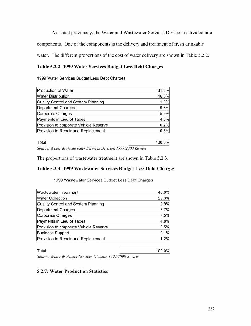
227

As stated previously, the Water and Wastewater Services Division is divided into

components. One of the components is the delivery and treatment of fresh drinkable

water. The different proportions of the cost of water delivery are shown in Table 5.2.2.

Table 5.2.2: 1999 Water Services Budget Less Debt Charges 1999 Water Services Budget Less Debt Charges Production of Water 31.3%Water Distribution 46.0%Quality Control and System Planning 1.8%Department Charges 9.8%Corporate Charges 5.9%Payments in Lieu of Taxes 4.6%Provision to corporate Vehicle Reserve 0.2%Provision to Repair and Replacement 0.5% Total 100.0%Source: Water & Wastewater Services Division 1999/2000 Review The proportions of wastewater treatment are shown in Table 5.2.3. Table 5.2.3: 1999 Wastewater Services Budget Less Debt Charges

1999 Wastewater Services Budget Less Debt Charges Wastewater Treatment 46.0%Water Collection 29.3%Quality Control and System Planning 2.9%Department Charges 7.7%Corporate Charges 7.5%Payments in Lieu of Taxes 4.8%Provision to corporate Vehicle Reserve 0.5%Business Support 0.1%Provision to Repair and Replacement 1.2% Total 100.0%Source: Water & Waster Services Division 1999/2000 Review 5.2.7: Water Production Statistics

228

In order to determine the costs of adaptation to climate change, information about

plant capacities, consumption and average daily flows are required. Tables 5.2.4 to 5.2.7

show relevant statistics on potable water production.

Table 5.2.4: Potable Water Production

Supply Plant Total Filt Percentage of Number of Days 1999 Average Maximum Daily Days of Water Produced Total in Pumpage Production Maximum (Mega litres) Operation (Megalitres per day) (Megalitres) Production Harris 251,898 44.7% 365 690 961 July 6, 1999 Clark 154,395 27.4% 355 434 632 August 26, 1999Horgan 142,858 25.4% 358 399 594 July 29, 1999 Island 14,350 2.5% 91 157 292 July 29, 1999 Total 563,502 Source: Water & Waster Services Division 1999/2000 Review Table 5.2.5: 1999 Water Consumption by Toronto Communities

1999 Water Consumption by Toronto Communities Communities Consumption Daily Average Population Per Capital Consumption

(Megalitres) (Megalitres) (Litres per day) East York 17,384 48 114,881 415 Etobicoke 71,037 195 350,240 556 North York 109,013 299 628,259 475 Scarborough 96,103 263 595,556 442 Toronto 150,309 412 696,535 591 York 22,986 63 156,128 403 Toronto Total 466,833 1,279 2,541,600 503 York Region Total 80,662 221 525,027 421 Total 547495 1,500 3,066,627 489 Source: Water & Waster Services Division 1999/2000 Review Table 5.2.6: Plant Capacities & Average Daily Flows

Plant Capacities & Average Daily Flows Plant Capacity Average Daily Flow

Square Meters per Day Square Meters per Day Ashbridges Bay 818,000 736,000 North Toronto 34,000 33,700 Highland Creek 218,000 168,100 Humber 472,000 364,510 Total 1,542,000,000 1,302,310,000 Source: Water & Waster Services Division 1999/2000 Review

229

Table 5.2.7: Pumping Station Capacities

Pumping Station Capacities Pumping Station Capacities Cubic Meters of Water per Day

Main 1,491,100 Ashbridges Bay 1,363,800 Cumber (Centennial) 68,200 West Rouge 31,800 Swansea 13,600 New Toronto 45,500 Long Branch 13,600 Mimico 68,200 Total 3,095,800 Source: Water & Waster Services Division 1999/2000 Review Table 5.2.8 gives the descriptive statistics of the projections of precipitation from

CGCM1, GG1, which we have downscaled for Toronto, following the methodology

given in Chapter 2.

Table 5.2.8: Precipitation Descriptive Statistics for Toronto

1961-2099 1961-1990 2010-2039 2040-2069 2070-2099 Maximum 1053.47 224.2 1053.47 1000.13 943.45 Minimum 2.12 10.1 3.66 2.12 3.83

Mean 88.56 75.61 92.96 89.27 96.42 Standard Deviation 78.98 34.43 96.25 83.29 85.83

Maximum precipitation increases from the baseline period to the 2020 period by a

factor of 4.7 and the mean increases by 23 percent in the same period. The standard

deviation increases a dramatic 179% from the baseline period to the 2020 period. It

remains 141% to 149% higher than the baseline in the 2050 and 2080 time periods,

respectively.

5.2.8: Regression Analysis

Given the average monthly precipitation for 1961-1990, 2010-2039, 2040-2069

and 2070-2099, for each period we estimate a regression model to analyze trend and

230

seasonal differences. The conceptual foundations of these regression models are given in

Chapter 2. The model takes the general form:

PPTt= β0 + β2 D2 + β3D3 +…β12D12 + u Where PPT is precipitation in period t, and the Di are dummy variables. The constant

represents January, D2 represents February and so on.

The estimated regression for 1961-1990 is:

PPT= 70 –6.39D2 +3.06D3 + 1.64D4 + 2.58D5 + 1.5D6 + 5.38D7 + 17.23D8 + 10.53D9 – (11.26) (-0.72) (0.34) (0.18) (0.29) (0.17) (0.61) (1.95) (1.19)

2.25D10 +12.83D11 + 21.16 D12

(-0.25) (1.45) (2.4)

The estimated regression for 2010-2039 is:

PPT= 83.27 –0.53D2 +1.27D3 – 1.35D4 – 8.66D5 – 14.73D6 + 24.06D7 + 4.18D8 + (4.7) (0.02) (0.05) (-0.05) (-0.34) (-0.59) (0.96) (0.16)

31.22D9 + 20.78D10 + 34D11 + 24.99D12 (1.25) (0.83) (1.36) (1)

The estimated regression for 2040-2069 is:

PPT= 77.16 + 1.57D2 + 16.04D3 + 13.89D4 + 4.87D5 – 6.47D6 + 29.84D7 – 4.02D8 + (5.05) (0.07) (0.74) (0.64) (0.22) (-0.3) (1.38) (-0.18)

37.08D9 + 20.76D10 + 22.09D11 + 9.75D12 (1.71) (0.96) (1.02) (0.45)

The estimated regression for 2070-2099 is:

PPT = 99.62 - 3.16D2 + 24.51D3 – 10.08D4 – 15.78D5 – 16.53D6 + 6.39D7 + 3.81D8 – (6.32) (-0.14) (1.09) (-0.45) (-0.7) (-0.74) (0.28) (0.17)

0.73D9 – 7.17D10 - 22.58D11 + 2.88D12 (-0.03) (-0.32) (-1.01) (0.12)

231

These regressions describe the relationship between precipitation and the constant

and eleven dummy variables. The constant represents the mean precipitation for January.

To determine the mean precipitation for any other month, the coefficient for that month is

added to or subtracted from the constant. We can see that the constant has increased in

each future scenario from the baseline. We can also see that the constant is significant in

every regression. These regressions are used to determine the mean and 95% confidence

interval around the mean. These results are graphed in Figures 5.2.2 to 5.2.5.

5.2.9: Graphical Results Figure 5.2.2: Results for Toronto (1961-1990)

Toronto 1961-1990

0

20

40

60

80

100

120

JAN FEB MAR APR MAY JUN JUL AUG SEP OCT NOV DECMonths

Crit ical Precipit at ion Level Lower Mean Upper

232

Figure 5.2.3: Results for Toronto (2010-2039) Figure 5.2.4: Results for Toronto (2040-2069)

Toronto 2010-2039

020406080

100120140160

JAN FEB MAR APR MAY JUN JUL AUG SEP OCT NOV DECMonths

Prec

ipita

tion

in m

m

Crit ical Precipit at ion Level Lower Mean Upper

Toronto 2040-2069

020406080

100120140160

JAN FEB MAR APR MAY JUN JUL AUG SEP OCT NOV DECMonthsPr

ecip

itatio

n in

mm

Crit ical Precipit at ion Level Lower Mean Upper

233

Figure 5.2.5: Results for Toronto (2070-2099)

In the graphs given in Figures 5.2.2 to 5.2.5 we are concerned with the mean and

the upper and lower 95% confidence levels, and their relationship to the critical

precipitation level. Note that the critical precipitation level can also be interpreted as the

maximum capacity of the wastewater treatment plant. That is, precipitation that exceeds

this level will cause the excess flow to be discharged untreated into Lake Ontario. We

can see that in the baseline scenario, mean precipitation does not exceed the capacity, but

the upper confidence level does in several months. The situation changes dramatically in

the future scenarios where mean and upper 95% level exceeds capacity more frequently.

This graphical representation allows us to see that increased precipitation will lead to

wastewater treatment problems due to insufficient capacity.

5.2.10: Methodology

If we assume that the average base year precipitation represents the average

precipitation for the Toronto area, then the amount of storm water requiring treatment

Toronto 2070-2099

0

50

100

150

200

JAN FEB MAR APR MAY JUN JUL AUG SEP OCT NOV DECMonths

Prec

ipita

tion

in m

m

Crit ical Precipit at ion Level Lower Mean Upper

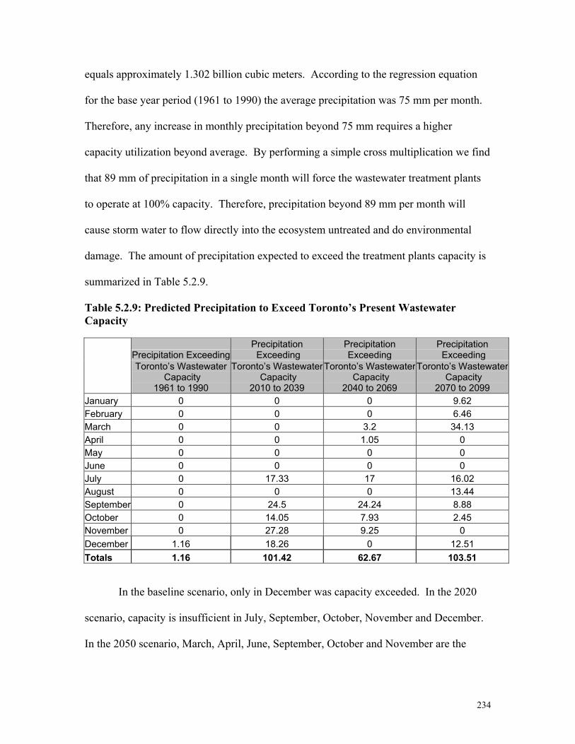
234

equals approximately 1.302 billion cubic meters. According to the regression equation

for the base year period (1961 to 1990) the average precipitation was 75 mm per month.

Therefore, any increase in monthly precipitation beyond 75 mm requires a higher

capacity utilization beyond average. By performing a simple cross multiplication we find

that 89 mm of precipitation in a single month will force the wastewater treatment plants

to operate at 100% capacity. Therefore, precipitation beyond 89 mm per month will

cause storm water to flow directly into the ecosystem untreated and do environmental

damage. The amount of precipitation expected to exceed the treatment plants capacity is

summarized in Table 5.2.9.

Table 5.2.9: Predicted Precipitation to Exceed Toronto’s Present Wastewater Capacity

Precipitation Exceeding Precipitation Exceeding

Precipitation Exceeding

Precipitation Exceeding

Toronto’s Wastewater Capacity

1961 to 1990

Toronto’s Wastewater Capacity

2010 to 2039

Toronto’s Wastewater Capacity

2040 to 2069

Toronto’s Wastewater Capacity

2070 to 2099 January 0 0 0 9.62 February 0 0 0 6.46 March 0 0 3.2 34.13 April 0 0 1.05 0 May 0 0 0 0 June 0 0 0 0 July 0 17.33 17 16.02 August 0 0 0 13.44 September 0 24.5 24.24 8.88 October 0 14.05 7.93 2.45 November 0 27.28 9.25 0 December 1.16 18.26 0 12.51 Totals 1.16 101.42 62.67 103.51

In the baseline scenario, only in December was capacity exceeded. In the 2020

scenario, capacity is insufficient in July, September, October, November and December.

In the 2050 scenario, March, April, June, September, October and November are the

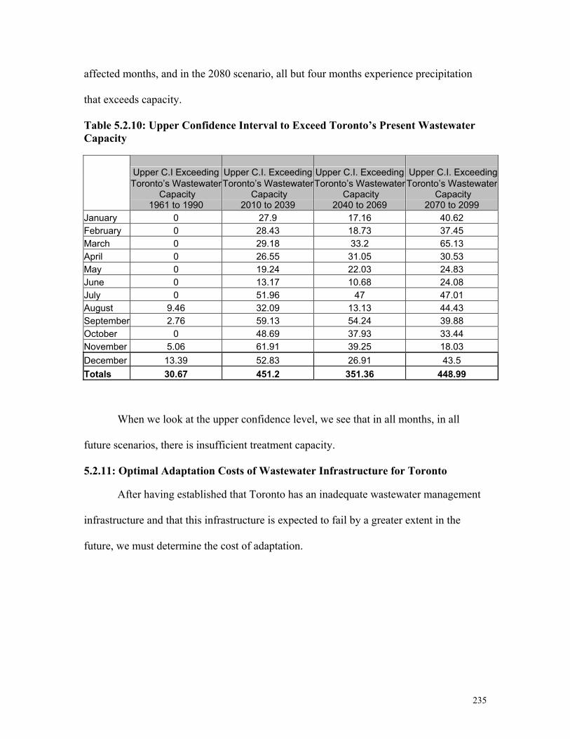
235

affected months, and in the 2080 scenario, all but four months experience precipitation

that exceeds capacity.

Table 5.2.10: Upper Confidence Interval to Exceed Toronto’s Present Wastewater Capacity

Upper C.I Exceeding Upper C.I. Exceeding Upper C.I. Exceeding

Upper C.I. Exceeding

Toronto’s Wastewater Capacity

1961 to 1990

Toronto’s Wastewater Capacity

2010 to 2039

Toronto’s Wastewater Capacity

2040 to 2069

Toronto’s Wastewater Capacity

2070 to 2099 January 0 27.9 17.16 40.62 February 0 28.43 18.73 37.45 March 0 29.18 33.2 65.13 April 0 26.55 31.05 30.53 May 0 19.24 22.03 24.83 June 0 13.17 10.68 24.08 July 0 51.96 47 47.01 August 9.46 32.09 13.13 44.43 September 2.76 59.13 54.24 39.88 October 0 48.69 37.93 33.44 November 5.06 61.91 39.25 18.03 December 13.39 52.83 26.91 43.5 Totals 30.67 451.2 351.36 448.99

When we look at the upper confidence level, we see that in all months, in all

future scenarios, there is insufficient treatment capacity.

5.2.11: Optimal Adaptation Costs of Wastewater Infrastructure for Toronto

After having established that Toronto has an inadequate wastewater management

infrastructure and that this infrastructure is expected to fail by a greater extent in the

future, we must determine the cost of adaptation.

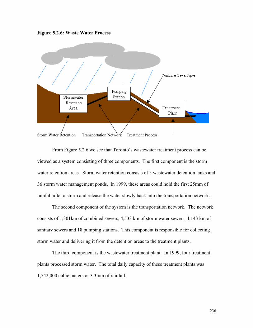
236

Figure 5.2.6: Waste Water Process

Storm Water Retention Transportation Network Treatment Process

From Figure 5.2.6 we see that Toronto’s wastewater treatment process can be

viewed as a system consisting of three components. The first component is the storm

water retention areas. Storm water retention consists of 5 wastewater detention tanks and

36 storm water management ponds. In 1999, these areas could hold the first 25mm of

rainfall after a storm and release the water slowly back into the transportation network.

The second component of the system is the transportation network. The network

consists of 1,301km of combined sewers, 4,533 km of storm water sewers, 4,143 km of

sanitary sewers and 18 pumping stations. This component is responsible for collecting

storm water and delivering it from the detention areas to the treatment plants.

The third component is the wastewater treatment plant. In 1999, four treatment

plants processed storm water. The total daily capacity of these treatment plants was

1,542,000 cubic meters or 3.3mm of rainfall.

237

Several different methods exist to build excess capacity into the wastewater

infrastructure. The Wastewater Services Division could construct one or more new

wastewater treatment plants, construct new water detention tanks (“storm water detention

tunnels”) or improve the efficiency of their existing treatment plants. In order to estimate

the cost of these improvements we have assumed that wastewater treatment technology is

constant. This simplification allows us to dismiss the third option and treat the problem

as a mixed-integer programming problem.

5.2.11.1: Experiment 1

By altering the capacity of storm water retention and treatment facilities the

wastewater infrastructure can adequately treat different volumes of precipitation. The

goal of our experiment is to minimize the total cost of infrastructure subject to the

expected level and distribution of precipitation. This experiment uses CGCM1, GG1

precipitation data for the entire Grid 445. This first experiment is without downscaling.

Let A represent the average daily precipitation in millimeters.

Let x represent the incremental water treatment capacity in millimeters per day.

Let y represent the incremental capacity of the holding tanks.

Then the mixed-integer programming problem for finding the optimal x and y is:

Min x,y C = 154.30x + 78.57y

A – x ≤ y y ≤ 2 5 x ≥ 3.3 x ≥ 0 y ≥ 0

A =5.53

238

Using the relationship 25x = 3.3y, we can eliminate y from the objective function

and using the Newton-Raphson method, find the optimal solution for x and y. The

solution is displayed in diagram 5.2.7.

Figure 5.2.7: Solution – Experiment 1

The blue line represents the total cost of increasing x and y. The optimal solution

x* and y* is the global minimum of this curve.

The optimal solution is x*=2, y*=0, where x* is the incremental change in storm

water treatment capacity and y* is the incremental change in storm water holding tanks in

millimeters of rainfall. That is, storm water treatment capacity increases by 2mm and the

storm water holding tanks continue to hold 25mm of precipitation.

5.2.11.2: Experiment 2

In this experiment, once again we took precipitation data for CGCM1 Grid 445

without downscaling and distributed precipitation normally over the month. Now the

mixed integer program problem is:

0500

100015002000250030003500

0 2 4 6 8 10

Increase in x

Cos

t

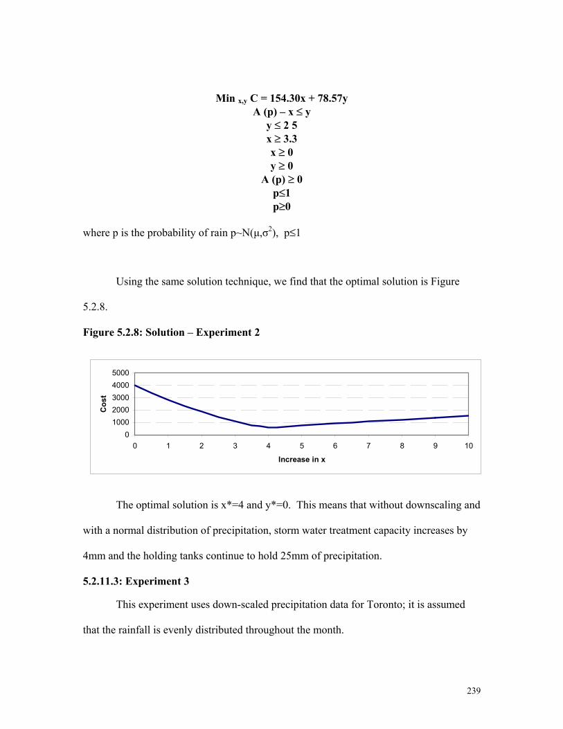
239

Min x,y C = 154.30x + 78.57y A (p) – x ≤ y

y ≤ 2 5 x ≥ 3.3 x ≥ 0 y ≥ 0

A (p) ≥ 0 p≤1 p≥0

where p is the probability of rain p~N(µ,σ2), p≤1

Using the same solution technique, we find that the optimal solution is Figure

5.2.8.

Figure 5.2.8: Solution – Experiment 2

The optimal solution is x*=4 and y*=0. This means that without downscaling and

with a normal distribution of precipitation, storm water treatment capacity increases by

4mm and the holding tanks continue to hold 25mm of precipitation.

5.2.11.3: Experiment 3 This experiment uses down-scaled precipitation data for Toronto; it is assumed

that the rainfall is evenly distributed throughout the month.

010002000300040005000

0 1 2 3 4 5 6 7 8 9 10

Increase in x

Cos

t

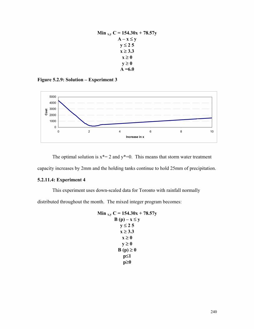
240

Min x,y C = 154.30x + 78.57y A – x ≤ y y ≤ 2 5 x ≥ 3.3 x ≥ 0 y ≥ 0

A =6.0 Figure 5.2.9: Solution – Experiment 3

The optimal solution is x*= 2 and y*=0. This means that storm water treatment

capacity increases by 2mm and the holding tanks continue to hold 25mm of precipitation.

5.2.11.4: Experiment 4

This experiment uses down-scaled data for Toronto with rainfall normally

distributed throughout the month. The mixed integer program becomes:

Min x,y C = 154.30x + 78.57y B (p) – x ≤ y

y ≤ 2 5 x ≥ 3.3 x ≥ 0 y ≥ 0

B (p) ≥ 0 p≤1 p≥0

0

1000

2000

3000

4000

5000

0 2 4 6 8 10

Increase in x

Cos

t

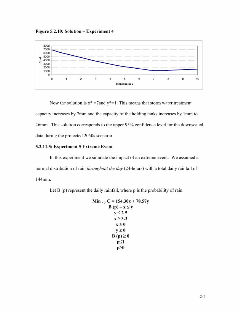
241

Figure 5.2.10: Solution – Experiment 4

Now the solution is x* =7and y*=1. This means that storm water treatment

capacity increases by 7mm and the capacity of the holding tanks increases by 1mm to

26mm. This solution corresponds to the upper 95% confidence level for the downscaled

data during the projected 2050s scenario.

5.2.11.5: Experiment 5 Extreme Event

In this experiment we simulate the impact of an extreme event. We assumed a

normal distribution of rain throughout the day (24-hours) with a total daily rainfall of

144mm.

Let B (p) represent the daily rainfall, where p is the probability of rain.

Min x,y C = 154.30x + 78.57y B (p) – x ≤ y

y ≤ 2 5 x ≥ 3.3 x ≥ 0 y ≥ 0

B (p) ≥ 0 p≤1 p≥0

010002000300040005000600070008000

0 1 2 3 4 5 6 7 8 9 10

Increase in x

Cos

t

242

Figure 5.2.11: Solution – Experiment 5

The optimal solution is x*=0and y*=116. This means that storm water treatment

capacity does not increase, but holding tank capacity increases by 116mm.

What do these experiments show? They show that wastewater treatment

infrastructure (i.e. treatment capacity plus storage capacity) depends heavily on the nature

of the distribution of precipitation. If rainfall is evenly distributed, then the optimal

solution is always to increase treatment capacity. If however, the distribution of rainfall

is such that the quantity of precipitation is greater than the treatment capacity, then it is

optimal to add to storage capacity.

An additional factor in the above solution is the cost of land. In Toronto we have

assumed the cost of land for holding tanks and storage to be $78.57 million per

millimeter of rainfall. To obtain this estimate we surveyed storm water infrastructure

costs in the state of California and multiplied the cost by 1.5 to obtain the cost in

Canadian dollars. In smaller Californian cities the cost of storm water retention was as

low as $43.18 million per millimeter of rain. We believe this lower cost is the result of

lower land costs and therefore is not representative of a major city, like Toronto.

5.2.12: Combined Sewers

90009200940096009800

10000

0 1 2 3 4 5 6 7 8 9 10

Increase in x

Cos

t

243

Although we have the ability to influence the cost of infrastructure by varying the

capacity of wastewater treatment and wastewater storage, one cost that cannot be avoided

is the conversion cost of separating combined sewers into separate sanitary and storm

sewer lines. During wet weather months the volume of storm water exceeds the capacity

of the wastewater treatment plants, which then causes the water in the sewers to mix. As

the backup continues the water eventually overflows untreated into Lake Ontario. To

solve this problem we have to construct separate sewers lines. The cost of this project

was estimated to be $271 million in 1992. In 1999, this cost has risen by approximately

20% to $325 million.

5.2.13: Total Cost of Adaptation

The adaptation cost to wastewater infrastructure is the low estimate (Experiment

1) based on an even distribution of precipitation throughout the month with no

downscaling.

Cost to increase wastewater capacity (2) $154.30 $308.60 Cost to increase wastewater storage (0) $78.57 Cost of sewer replacement $325.00

Total $633.60

Therefore, using precipitation data for Grid 445, the total adaptation cost is

$633,600,000. This is based on a 2mm increase in wastewater treatment capacity and no

change in the holding tank storage capacity. The cost of sewer replacement is an actual

cost based on previous sewer replacements.

The high estimate (Experiment 5) is based on an extreme event.

244

Cost to increase wastewater capacity (0) $154.30 Cost to increase wastewater storage (116) $78.57 $9,114.12 Cost of sewer replacement $325.00

Total $9,439.12

Therefore, the cost of adaptation to an extreme event is equal to the cost of

increasing holding tank storage plus the cost of sewer replacement. In the case of

Toronto, the cost of adaptation is equal to $9,439,120,000, depending on how risk averse

Toronto is. It should also be noted that throughout this study no discounting is used.

5.2.14: Summary and Conclusion

We conclude that the City of Toronto will face adaptation costs from a low of

$633 million to a high of $9.4 billion. These are the costs associated with increasing

wastewater treatment and storage capacity, as it seems likely that in the future scenarios,

precipitation will increase beyond the existing capacity. Drinking water supply does not

appear to be affected by climate change, as intake pipes are deeper than the expected 1

metre drop in lake levels.

5.3: Niagara, ON

In Niagara, the water distribution system consists of eight potable water systems,

including seven water treatment plants and one well system together with the associated

flow metering facilities, water mains, reservoirs, tanks and pumping stations. Water

treatment consists of screening, coagulation, flocculation, sedimentation, pH correction

245

and rapid gravity filtration. Granular activated carbon filter-adsorbers are used for taste

and odour control, as well as powdered activated carbon.

There is an estimated $110 billion of in-ground water infrastructure assets in

Canada and there is a population of approximately 30 million people. Therefore the per

capita investment in water infrastructure in Canada is $3667. The population of the

Region of Niagara is 415,600 (see Figure 5.2.1). Therefore, the estimated value of the

water infrastructure in Niagara is about $1.5 billion.

Drinking water production in Niagara ranges from an actual high of 89,981,408

cubic metres (89,981,408,000 litres) in 1988 to a projected low of 61,327,047 cubic

metres (61,327,047,000 litres) in 2010. The numbers indicate that there will be an

average decrease in production of –1.63%. The average daily demand for water in litres

per capita ranges from a low in 1997 of 539.843 to a high of 592.062 in 1991.

In the Region of Niagara, the Water & Wastewater division is responsible for the

operation and engineering of water and sewer systems. The division is also accountable

for master servicing plans, water & sewer approvals, laboratory services, environmental

monitoring, industrial waste and training. The Region has the responsibility for the

domestic water supply (including pumps, storage facilities and 39.5 km. of mains) and

sewage treatment facilities (including pumping stations and forcemains). Water treatment

is the process of cleaning and disinfecting water, and because water is a natural solvent, it

attracts various pollutants and is not always safe to drink. The Region of Niagara

operates and maintains eight potable water systems that include seven water treatment

plants and one well system together with the associated remote treatment and flow

metering facilities, water mains, storage reservoirs and tanks, and pumping stations. The

246

systems vary in capacity from 227.3 ML/d to 4.3 ML/d. The total rated normal capacity

for all potable water systems is 613.6 ML/d. In addition, screened raw water is supplied

to the City of Thorold for industrial users.

A total of 80,717,236 cubic metres of potable water and 1,225,405 cubic metres

of raw water were supplied by the various systems in 1998. Compared to the previous

year this is a 5.6 percent increase in potable water and a 3.6 percent increase in the

industrial raw water. The actual net expenditure for water operations, including

administration and supervision, was $8,442,702. The uniform water rate for potable water

was $ 1.25 per 1,000 gallons ($ 0.275 per cubic metre). The rate charged to the City of

Thorold for raw water was $0.00605 per 1,000 gallons ($0.0013 per cubic metre) for

system operation.

In 1999, a total of 81,014,957 cubic metres of potable water and 489,915 cubic

metres of raw water were supplied. Compared to 1998, this is a 0.5 percent increase in

potable water and a 61 percent decrease in the industrial raw water. In 1999, the actual

net expenditure for water operations, including administration and supervision, was

$8,868,559. The uniform rate for potable water was $1.323 per 1,000 gallons ($0.2910

per cubic metre).

5.3.1: Precipitation Trends In 1999, total precipitation across Niagara was well below the normal as defined

by Meteorological Services of Canada (MSC) of Environment Canada. The winter of

1998/1999 saw the beginning of a dry trend with well below normal precipitation in

January and February. The Spring experienced the same trend with March being 80%

below normal and April and May, 20 to 40% dryer than normal. A limited degree of

variability in precipitation patterns was observed in the summer; however June and July

247

were 40% below MSC normals and August was 30% below normal. Above normal

precipitation values were observed in the fall, with three storms accounting for 60 to 70%

of the rainfall for the season.

5.3.2: Precipitation and Water Flow In 1999, the Niagara Region average monthly rainfall exceeded the MSC average

monthly rainfall in September, October and November. The seven-year average monthly

rainfall trend, from 1993 to 2000 was below the MSC average monthly rainfall except for

December 1995, summer of 1996 and the winter of 1996. In 1999, the regional average

precipitation was 578mm and the actual water flow was 81,014,957 cubic metres.

5.3.3: Niagara River Drainage, Lake Erie and Lake Ontario The Niagara River drains an area of 254,708 square miles, including the Upper

Great Lakes. The surface area of Lake Erie is 87,845 square miles, and it is the

shallowest of the Great Lakes, averaging 60 feet in depth. The levels of the Great Lakes

vary on an annual basis in relation to the season, rainfall, evaporation and runoff. The

highest water levels occur in mid-summer and the lowest occur in mid-winter. The

internal time required for an increase supply of water to show its effect upon the level of

Lake Erie is approximately 76 days. The internal time required for a decrease in the

supply of water to show its effect upon the level of Lake Erie is approximately 132 days.

A variation in the level of Lake Erie of one foot at Buffalo, New York equates to a

difference in the rate of flow discharge from Lake Erie into the Niagara River of 20,000

to 25,000 cubic feet per second. During storms, the water level of Lake Erie may vary as

much as 15 feet. The average annual rainfall in the Great Lakes equals 36 inches, and the

average annual evaporation rate equals 24 inches. In September 1999, water level at

Lake Erie was at 571.19 feet above sea level. This was 4.3 inches (11 cm) below the

248

long-term average. Lake Erie’s water level was the lowest that has been recorded since

1967. In the summer of 1999, the Great Lakes water levels were 16-24 inches below

those recorded in 1998. The average flow water rates are shown in Table 5.3.2.

Table 5.3.1: Average Flow Water Rates Time Period Inflow (Lake Erie into Niagara River) Outflow (from Niagara River)

Sept.1999-Feb.2000 173,400 cubic ft/sec. 184,000 cubic ft/sec.

Mar-Aug1999 186,100 cubic ft/sec. 200,660 cubic ft/sec.

5.3.4: Drinking Water Supply Impacts 5.3.4.1: Capital Costs The decrease in net precipitation results in a decrease in lake levels. This could

have an impact on water supply, as water intake pipes must be either extended or moved

in order to draw enough water of suitable quality. The Niagara Region has water intake

pipes in Lake Ontario, Lake Erie, Niagara River via the Welland River Channel and Lake

Erie via the Welland Canal.

The intake pipes that could be affected by lower lake levels are those in Lake Erie

and Lake Ontario. The Lake Erie pipe is at a depth of 20 feet and extends about 800

metres into the lake. The Lake Ontario pipe is at a depth of 30 feet and extends 1950

metres into the lake.

Because the pipes are deep and extend so far into the lake, a decrease of 1 metre

in lake level may not have an appreciable effect on the ability of the intake pipes to

access suitable water. However, the marginal costs of adding pipe are calculated below

in the event that water levels drop so far that additional pipes are needed to draw water.

5.3.4.2: Operating Costs Lower lake levels might have an impact on operating costs in terms of raw water

249

treatment. Higher evaporation rates will leave more suspended solids in raw water,

increasing the water treatment costs. To estimate the costs of increased treatment due to

a higher number of suspended solids, annual treatment costs and lake levels can be

compared. This is a subject for future research.

5.3.4.3: Capital Projects

In 1999, capital projects carried out in the Niagara peninsula in the water supply

system amounted to $16,500,000 and for 2001 the amount is budgeted at $17,400,000.

Capital cost outlays can include water treatment plant upgrades, raw water supply

improvements, reservoir connection piping, and booster pumping station upgrades, water

main replacements and storage tank replacements.

5.3.5: Wastewater Treatment 5.3.5.1: Climate Induced Change in the Rainfall

The Region of Niagara operates and maintains fourteen wastewater systems that

include nine full wastewater treatment plants, one lagoon augmented with

chemical/physical treatment and four lagoon systems together with the associated flow

metering facilities, force mains, gravity sewers, storage tanks, and pumping stations. The

system consists of 103 Regional Niagara owned and/or operated pumping stations, 7

owned and operated by the municipalities, 3 odour control stations, 4 metering chambers

and 1 storm water holding reservoir. In 1998 the quantity of sewage treated at Niagara’s

wastewater treatment plants was 84,083,335m3. In 1999 this figure was 83,444,822m3, a

.76% decrease. The systems vary in capacity from 68,200 m3/d to 500 m3/d. The full

treatment capacity rating for all wastewater systems is 329,880m3/d. The peak storm

rating for all systems is 707,480m3/d. The actual net expenditure for wastewater

operations, including administration and supervision was $15,671,597 in 1999. The

250

uniform water rate for wastewater treatment was $2.178 per 1,000 gallons ($0.4790 per

cubic metre).

Wastewater flows in Niagara range from an actual high of 102,922,624 cubic

metres (102,922,624,000 litres) in 1996 to a low of 77,050,775cubic metres

(77,050,775,000 litres) in 1988. The numbers indicate that there will be an average

increase in flow of 1.6%. The average daily sewage per capita ranges from a low in 1988

of 492.562 litres to a high of 697.728litres in 1996. The Region of Niagara has projected

sewage flows to increase over the next decade. The average daily projected sewage

flows in litres for the next decade are:

2001 266,030,443.8 2002 268,118,580.8 2003 270,206,720.5 2004 272,294,857.5 2005 274,382,997.3 2006 276,471,134.2 2007 278,559,274.0 2008 280,647,411.0 2009 282,735,550.7 2010 284,823,687.7

Periods of high precipitation cause an increase in sewage generation, due to the

influx of extraneous flows via inflow and infiltration and resulting wet weather flows. In

2000, the Region experienced an increase in precipitation from 30mm to 160mm from

January to June. In the same period sewage flows increased from 7,000,000 cubic metres

to 10,000,000 cubic metres. Precipitation dropped from a high of 160mm in June to

55mm in July, and sewage flow similarly declined from 10,000,000 cubic metres to

7,000,000 cubic metres.

5.3.5.2: General Circulation Model-CGCM1 Greenhouse Gas Only Simulation

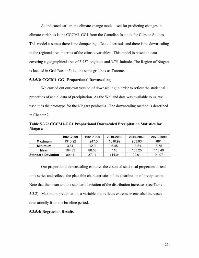
251

As indicated earlier, the climate change model used for predicting changes in

climate variables is the CGCM1-GG1 from the Canadian Institute for Climate Studies.

This model assumes there is no dampening effect of aerosols and there is no downscaling

to the regional area in terms of the climate variables. This model is based on data

covering a geographical area of 3.75o longitude and 3.75o latitude. The Region of Niagara

is located in Grid Box 445; i.e. the same grid box as Toronto.

5.3.5.3: CGCM1-GG1 Proportional Downscaling

We carried out our own version of downscaling in order to reflect the statistical

properties of actual data of precipitation. As the Welland data was available to us, we

used it as the prototype for the Niagara peninsula. The downscaling method is described

in Chapter 2.

Table 5.3.2: CGCM1-GG1 Proportional Downscaled Precipitation Statistics for Niagara

1961-2099 1961-1990 2010-2039 2040-2069 2070-2099 Maximum 1310.92 247.5 1310.92 933.93 881 Minimum 3.61 12.9 6.45 3.61 6.75

Mean 104.33 88.58 110 105.25 113.49 Standard Deviation 89.44 37.11 114.04 92.01 94.07

Our proportional downscaling captures the essential statistical properties of real

time series and reflects the plausible characteristics of the distribution of precipitation.

Note that the mean and the standard deviation of the distribution increases (see Table

5.3.2). Maximum precipitation, a variable that reflects extreme events also increases

dramatically from the baseline period.

5.3.5.4: Regression Results

252

To find the monthly pattern of precipitation, we regressed precipitation on eleven

monthly dummy variables. The conceptual foundation for these regressions is given in

Chapter 2.

The estimated regression for 1961 to 1990 is:

PPT= 87.72 – 5.36D2 – 2.6D3 – 6.61D4 – 9.94D5 + 3.19D6- 14.14D7 + 5.01D8 + (13.38) (-0.57) (-0.28) (-0.71) (-1.07) (0.34) (-1.52) (0.54)

4.95D9 – 6.23D10 + 11.45D11+ 30.65D12 (0.53) (-0.67) (1.23) (3.3)

The estimated regression for 2010 to 2039 is: PPT= 101.1 + 5.13D2 + 16.24D3 – 3.15D4 – 20.86D5 – 10.57D6 + 13.14D7 – 9.94D8 (4.86) (0.17) (0.55) (-0.1) (-0.7) (-0.35) (0.44) (-0.33)

+ 19.93D9 + 22.77D10 + 42.19D11 + 48.27D12 (0.65) (0.77) (1.43) (1.64)

The estimated regression for 2040 to 2069 is: PPT= 92.6 + 8.97D2 + 15.03D3 + 14.28D4 – 3.18D5 + 3.13D6 + 17.23D7 – 11.9D8 + (5.48) (0.37) (0.62) (0.59) (-0.13) (0.13) (0.72) (-0.49) 31.99D9 + 25.45D10 + 27.2D11 + 23.38D12 (1.33) (1.06) (1.13) (0.97)

The estimated regression for 2070 to 2099 is: PPT= 128.88 – 4.77D2 + 15.88D3 – 21.11D4 – 42.63D5 – 20.15D6 –25.54D7 –27.79D8 (7.5) (-0.19) (0.65) (-0.86) (-1.75) (-0.83) (-1.05) (-1.14)

– 17.14D9 – 20.4D10 – 32.49D11 + 11.49D12 (-0.7) (-0.84) (-1.33) (0.47)

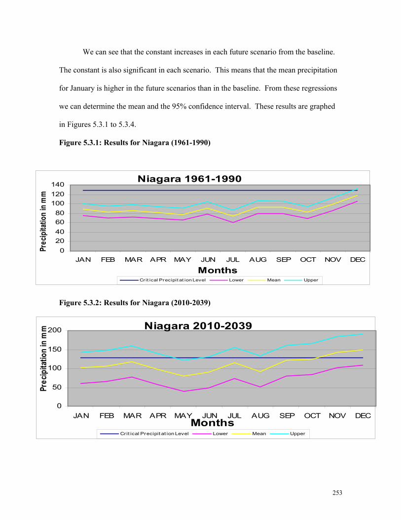
253

We can see that the constant increases in each future scenario from the baseline.

The constant is also significant in each scenario. This means that the mean precipitation

for January is higher in the future scenarios than in the baseline. From these regressions

we can determine the mean and the 95% confidence interval. These results are graphed

in Figures 5.3.1 to 5.3.4.

Figure 5.3.1: Results for Niagara (1961-1990) Figure 5.3.2: Results for Niagara (2010-2039)

Niagara 1961-1990

020406080

100120140

JAN FEB MAR APR MAY JUN JUL AUG SEP OCT NOV DEC

Months

Prec

ipitat

ion in

mm

Crit ical Precipit at ion Level Lower Mean Upper

Niagara 2010-2039

0

50

100

150

200

JAN FEB MAR APR MAY JUN JUL AUG SEP OCT NOV DECMonths

Prec

ipita

tion

in m

m

Crit ical Precipit at ion Level Lower Mean Upper

254

Figure 5.3.3: Results for Niagara (2040-2069)

Figure 5.3.4: Results for Niagara (2070-2099)

In the baseline scenario, the mean does not exceed the capacity in any month, but

in the 2020 scenario the mean exceeds the capacity in November and December. The

mean also exceeds the capacity in several months of the 2080 scenario. As was the case

in the Toronto study, the upper confidence level exceeds the capacity in almost all

Niagara 2040-2069

0

50

100

150

200

JAN FEB MAR APR MAY JUN JUL AUG SEP OCT NOV DECMonths

Prec

ipita

tion

in

mm

Crit ical Precipit at ion Level Lower Mean Upper

Niagara 2070-2099

0

50

100

150

200

JAN FEB MAR APR MAY JUN JUL AUG SEP OCT NOV DECMonths

Prec

ipita

tion

in

mm

Crit ical Precipit at ion Level Lower Mean Upper

255

months of the future scenarios.

5.3.5.5: Capacities and Flows

Table 5.3.3 shows the capacity ratings and average daily flows of all Niagara

Region wastewater treatment plant facilities and lagoons.

Table 5.3.3: Wastewater Treatment Plant and Lagoon Flow Ratings Facility Rating m3/d Peak Storm Rating m3/d Average Daily Flow m3/d

Niagara Falls 68,200 136,400 56,822

Queenston 500 700 213.723

Port Dalhousie 61,350 122,700 40,722.173

Port Weller 68,100 136,200 41,475.367

Niagara-on-the-Lake 5,710 8,520 3841.444

Welland 54,550 136,200 42,784.129

Grimsby 22,750 45,460 16,336.811

Port Colborne 15,120 45,000 11,317.603

Fort Erie 24,500 49,000 10,946.477

Crystal Beach 9,100 27,300 3,048.597

Biggar 1,818.4 1,154.036

Port Robinson 441 267.981

Stevensville 2,273 1,069.602

Total 334,412.4 707,480 229,999.943

Source:Regional Municipality of Niagara Public Works Department 1999 Statistical Report

Average daily flow divided by capacity rating is equal to 68.7%

(229,999/334,412). The mean precipitation for 1961 to 1990 is 88.48mm. A simple

calculation will show that the precipitation level in a single month that will force the

treatment plants to operate at 100% is 128 mm. Therefore, precipitation beyond 128mm

a month will cause storm water to overflow into the ecosystem. That is, 128*.687 = 88.

The amount of precipitation expected to exceed the treatment plants’ capacity is

summarized in the following tables.

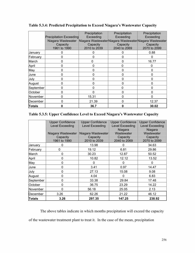
256

Table 5.3.4: Predicted Precipitation to Exceed Niagara’s Wastewater Capacity

Precipitation ExceedingPrecipitation Exceeding

Precipitation Exceeding

Precipitation Exceeding

Niagara Wastewater Capacity

1961 to 1990

Niagara Wastewater Capacity

2010 to 2039

Niagara Wastewater Capacity

2040 to 2069

Niagara Wastewater Capacity

2070 to 2099 January 0 0 0 0.88 February 0 0 0 0 March 0 0 0 16.77 April 0 0 0 0 May 0 0 0 0 June 0 0 0 0 July 0 0 0 0 August 0 0 0 0 September 0 0 0 0 October 0 0 0 0 November 0 15.31 0 0 December 0 21.39 0 12.37 Totals 0 36.7 0 30.02 Table 5.3.5: Upper Confidence Level to Exceed Niagara’s Wastewater Capacity

Upper Confidence Level Exceeding

Upper Confidence Level Exceeding

Upper Confidence Level Exceeding

Upper Confidence Level Exceeding

Niagara Wastewater Capacity

1961 to 1990

Niagara Wastewater Capacity

2010 to 2039

Niagara Wastewater

Capacity 2040 to 2069

Niagara Wastewater

Capacity 2070 to 2099

January 0 13.98 0 34.63 February 0 19.12 6.81 29.86 March 0 30.23 12.87 50.52 April 0 10.82 12.12 13.52 May 0 0 0 0 June 0 3.41 0.97 14.47 July 0 27.13 15.08 9.08 August 0 4.04 0 6.83 September 0 33.38 29.84 17.48 October 0 36.75 23.29 14.22 November 0 56.18 25.05 2.13 December 3.26 62.26 21.22 46.12 Totals 3.26 297.35 147.25 238.92

The above tables indicate in which months precipitation will exceed the capacity

of the wastewater treatment plant to treat it. In the case of the mean, precipitation

257

exceeds capacity in November and December of the 2020 scenario and January, March

and December of the 2080 scenario. In the case of the upper confidence interval,

precipitation exceeds capacity in almost every month of the future scenarios.

5.3.5.6: Capital Costs

Capital cost outlays can include trunk sewer replacement, sewer system upgrade,

sanitary sewer replacement, pumping station improvements and biosolids facility

improvements. In 1999, capital cost spending on the wastewater system was $15.1

million. A significant portion of the total costs of wastewater is driven by capital costs.

In wastewater, increased spending might be needed to accelerate wet weather flow

control and minimize overflows. Increased precipitation will cause an increase in sewage

flows. More containment tanks or separate storm and sanitary sewers will be needed.

5.3.6: Costs of Adaptation

The costs of adaptation for Niagara can be estimated using the same methodology

as Toronto, but research needs to be done into costs specific to Niagara. For a rough

estimate, we can use a rule-of –thumb approach by determining the extent to which the

wastewater treatment plant must increase capacity.

Tables 5.3.4 and 5.3.5 show precipitation exceeding capacity to be at its greatest

in the 2020 scenario. Maximum precipitation occurs in December when the mean

precipitation exceeds capacity by 21.39 mm and the 95% upper confidence level is

62.26mm. The wastewater treatment has a capacity of 128 mm of precipitation.

Therefore the capacity would have to expand a minimum of 16% and a maximum of 48%

to prevent wastewater overflow. Based on the 1999 capital spending figure of $15.1

million, capital spending in the 2020 scenario, for any given year, would have to increase

by $2.4 million to $7.2 million.

258

Based on an estimate of new wastewater treatment facilities costing $50 million

(see Section 5.10.2), the costs of expanding capacity range from $8 million to $24

million.

5.3.7: Summary and Conclusion In the Niagara Region, drinking water supply will not be affected by climate

change in the next century. The water supply comes from Lake Erie and Lake Ontario

and because lake levels will not fall below the depth of the intake pipes, water supply will

remain secure. This, of course, assumes that the levels of water in the Great Lakes do not

fall appreciably.

However, the capacity of wastewater treatment will be insufficient in the three

future scenarios. The upper 95% confidence intervals indicate that wastewater flows will

exceed treatment capacity. Therefore the costs of adaptation are those associated with

expanding wastewater treatment plants.

These costs were estimated to be in the range of $8 million to $24 million for an

investment in expansion of the wastewater treatment facilities and $2.4 million to $7.4

million on annual capital expenditures.

5.4: Montreal, PQ 5.4.1: Drinking Water Supply

In the Communauté Urbaine de Montréal, the water is drawn from the St.

Lawrence River and the average consumption of water per person per day is 1430 litres

(see Figure 5.4.1). This figure is double that of Toronto and three times that of

Edmonton. Annual consumption from 1995 to 1999 in thousands of cubic metres is as

follows:

259

1995 647,348 1996 638,125 1997 618,112 1998 633,067 1999 649,763 Source: Communauté urbaine de Montréal General Statistics

Figure 5.4.1: Communité Urbaine de Montréal

5.4.2: CGCM1-GG1 Proportional Downscaling

As in the previous section, we downscaled the data for Montreal using the

methodology described in Chapter 2. We used Grid box 411, which includes much of

southwestern Ontario, including Montreal. Table 5.4.1 shows the descriptive statistics

for precipitation.

3 0 0 3 0 6 0 K i l o m e t e r s

N

EW

S

G r i d B o x 4 1 1 - C o m m u n i t e U r b a i n e d e M o n t r e a l

260

Table 5.4.1: CGCM1-GG1 Proportional Downscaled Descriptive Precipitation Statistics

1961-2099 1961-1990 2010-2039 2040-2069 2070-2099 Maximum 534.96 234 534.96 388.65 402.57 Minimum 11.99 16.3 11.99 12.11 14.18

Mean 98.91 89.9 100.05 102.3 103.36 Standard Deviation 62.22 37.4 66.88 69.78 68.22

Note that the mean increases slightly over the four time periods and the standard

deviation increases 78.8% from the baseline scenario to the 2020 scenario. The

maximum increases from the baseline to the 2020 scenario by 128%, decreases in the

subsequent years but remains 66% to 72% above the baseline.

Based on this analysis, precipitation is expected to increase in the next one

hundred years, and so Montreal is unlikely to face droughts. Therefore we assume that

water supply is not expected to be adversely affected by a changing climate.

5.4.3: Wastewater Treatment

Some 180 outfalls located throughout the island of Montreal drain the

Communauté Urbaine de Montréal. The outfalls in the northern part of the territory used

to drain their wastewater into rivière des Prairies and lac les Deux Montagnes, but since

1984, it has been directed toward the Plant via the northern interceptor (41km).

Similarly, wastewater from the outfalls located in the southwestern area of the territory

was discharged into Lac Saint-Louis until 1987. Since then, it has been directed toward

the Plant through the southwestern interceptor (18 km), which is hooked up to the

northern interceptor. Wastewater from the remaining outfalls located in the southern area

of the territory was discharged into the Saint-Laurent until 1990. Since that time, it was

progressively channelled to the Plant as work on the southeastern interceptor (30.5 km)

was completed. The northern, southwestern and southeastern interceptors, which

261

measure a total of 89.5 km in length, constitute the Community’s wastewater interception

network. Their diameter varies from 1.8 to 5.4 metres. Since August 1995, the

Community’s Treatment Plant has processed, in dry weather flow periods, all of the

wastewater from the islands of Montreal and Bizard.

The average flow rate received at the Treatment Plant is approximately 2,500,000

m3/d. During heavy rainfalls, the wastewater flow rate can reach a maximum of

7,600,000 m3/d. The drainage networks for approximately one third of Montreal’s

territory, mainly the western sector, were developed as part of a separate system. The

latter is made up of a sanitary sewer for collecting residential, industrial, commercial and

institutional wastewater and a storm water sewer for rainwater. The drainage networks in

the remaining central and eastern sectors were almost exclusively developed as part of a

combined system with a single sewer collecting all wastewater and rainwater. The

Community’s interception network and the Wastewater Treatment Plant were built to

collect and treat approximately 75% of all rainwater from the combined system’s

drainage networks, representing 50% of all rainwater from the whole of the Montreal

area. About 60% of the territory is developed in a combined system. Each interception

structure can collect from 12 to 40 times the average dry weather flow. The

supplementary volume of water from rainwater accounts for about 13% of the total

volume of wastewater treated at the plant. This volume of water is negligible compared

to that from infiltration, which is estimated at more than 30% of the waters found at the

plant.

Directly connected to the interceptors, the 68 hookup structures (36 of which are

equipped with regulating structures) direct wastewater from the trunk sewers through the

262

interceptors to the Wastewater Treatment Plant. The hookup structures for the sanitary

trunk sewers are equipped with a diversion structure and a drop shaft linked to the

interceptor. Wastewater is being collected at all times.

In the case of the combined trunk sewers, the total flow rate is diverted toward the

interceptor during dry weather flow periods. However, during periods of heavy rainfall,

some of the runoff and wastewater may be channelled directly toward Rivière des

Prairies or the St. Lawrence River.

The diversion structure consists of a diversion box built under the invert of the

trunk sewer. In the event the trunk sewer should become submerged or affected by the

water level of the receiving waterway at the interception point, a flap gate chamber is

added to the trunk sewer to prevent the collection of water from the receiving waterway.

During rainy weather, sluice gates mounted in the regulating structure control the inflow

of wastewater and rainwater to the interceptor in response to signals from the control

centre at the Wastewater Treatment Plant or the local control panel. The wastewater is

directed toward a drop shaft, up to 30 metres deep, to the interceptor and flows by gravity

to the Wastewater Treatment Plant, located on the eastern tip of the island of Montreal.

The water is treated at the Plant, before being returned to the St. Lawrence.

The pumping station has a maximum capacity flow rate of 88 cubic metres per

second. When wastewater reaches the Plant, it is brought up to the surface by 17 pumps

and discharged into a peripheral channel. Eight of these pumps, each with a 6.3 m3/s

capacity, service the northern interceptor, while nine others, with a 6.9 m3/s capacity,

serve the southern interceptor.

263

The daily capacity of the wastewater treatment plant is 7.6 million cubic metres

per day and the average flow rate received at the plant is approximately 2.5 million cubic

metres per day. This capacity of 7.6 million cubic metres per day makes the Montreal

Wastewater Treatment Plant the largest primary physico-chemical treatment plant in

North America. Because on a given day, only 32% of the capacity of plant is utilized,

Montreal has a great deal of excess capacity already built into the system. During heavy

rainfalls, when the wastewater flow can reach 7.6 million cubic metres per day, 100% of

plant capacity is utilized. In the baseline period, the maximum amount of precipitation

was 234mm, and the mean was 89.9mm. By a simple calculation, we can conclude that

the maximum amount of precipitation the plant can treat is 280mm. Any precipitation

exceeding this amount will be discharged into the river, untreated. Before the

construction of this facility, wastewater was dumped directly into the St. Lawrence. The

Plant treats 44% of all wastewater processed in treatment plants within Quebec and has

one of the highest pumping capacities in all of North America (see Table 4.5.2).

Table 5.4.2 Average Flows and Treated Volumes

Average Flow (m3/s) Pumped Volume (Mm3) Average Daily Flow (m3)

Jan 30.2 80,904 2,609,800 Feb 29.3 75,879 2,709,900 Mar 28.9 69,796 2,251,400 Apr 34.1 91,248 3,041,600 May 25.3 67,706 2,184,000 Jun 28.1 72,825 2,427,500 Jul 28.3 75,683 2,441,000 Aug 27.1 72,681 2,344,500 Sept 33.9 87,915 2,930,500 Oct 31.0 82,976 2,676,600 Nov 25.0 64,835 2,161,000 Dec 29.5 79,068 2,550,000

Average 29.25 Total 921,516 Source: MUC Water and Wastewater website; www.cum.qc.ca/sewage

264

5.4.4: Wastewater Treatment Plant Costs

The total cost of this major wastewater treatment project required an investment

of $1.375 billion, of which $750 million was invested in the construction of the

Wastewater Treatment Plant and $625 million in the construction of the interceptor

network.

In 1998, the operational costs of the treatment plant were $42,909,500.

$16,212,000 are variable costs, which represent about 38% of the total operating costs.

Capital expenditures on sewers from 1995 to 1999 are:

1995 $28,406,000 1996 37,787,000 1997 18,084,000 1998 10,235,000 1999 8,599,000 Source: Ville de Montréal Capital Expenditure Fund

5.4.5: Regression Results

As with the other case studies, we now carry out some regressions to consider the

change in the pattern of precipitation for Montreal. The conceptual foundation for these

regressions is given in Chapter 2. The estimated regression for the 1961 to 1990 period

is:

PPT=73.73 – 3.01D2 + 8.9D3 + 5.76D4 + 8.91D5 + 19.93D6 + 26.27D7 + 33.39D8 + (11.23) (-0.32) (0.95) (0.62) (0.96) (2.14) (2.83) (3.59)

21.86D9 + 8.83D10 + 28.33D11 + 35.02D12

(2.35) (0.95) (3.05) (3.77)

The estimated regression for the 2010 to 2039 period is:

265

PPT= 68.61 + 18.02D2 + 34.39D3 + 19.96D4 + 22.57D5 + 40.24D6 + 37.25D7 (5.66) (1.05) (2) (1.16) (1.31) (2.35) (2.17)

39.33D8 + 36.58D9 + 44.15D10 + 25.29D11 + 59.5D12 (2.29) (2.13) (2.57) (1.47) (3.47)

The estimated regression for the 2040 to 2069 period is:

PPT= 78.96 + 4.19D2 + 24.56D3 + 30.75D4 + 18.93D5 + 28.67D6 + 21.59D7 + 1.37D8 (6.18) (0.23) (1.36) (1.7) (1.04) (1.58) (1.19) (1.18)

+ 22.86D9 + 38.45D10 + 27.63D11 + 41.04D12 (1.26) (2.13) (1.53) (2.27)

The estimated regression for the 2070 to 2099 period is:

PPT= 76.35 + 21.1D2 + 39.05D3 + 41.38D4 + 21.18D5 + 39.16D6 + 31.11D7 + 5.71D8

(6.17) (1.2) (2.23) (2.36) (1.21) (2.24) (1.78) (0.89)

+ 18.18D9 + 31.3D10 + 11.32D11 + 54.56D12 (1.04) (1.79) (0.64) (3.12)

These results indicate the mean precipitation in January (the constant) decreases

in the 2020 scenario then increases in 2050 and 2080. The constant is significant in all

scenarios.

The four regression results are plotted in Figures 5.4.2 to 5.4.5 respectively.

Figure 5.4.2: Results for Montreal (1961-1990)

Montreal 1961-1990

050

100150200250300

JAN FEB

MARAPR

MAY JUN JULAUG SEP

OCTNOV DEC

Months

Prec

ipitat

ion in

mm

Crit ical Precipit at ion Level Lower Mean Upper

266

Figure 5.4.3: Results for Montreal (2010-2039)

Figure 5.4.4: Results for Montreal (2040-2069)

Montreal 2010-2039

050

100150200250300

JAN FEB MAR APR MAY JUN JUL AUG SEP OCT NOV DECMonths

Prec

ipita

tion

in

mm

Crit ical Precipit at ion Level Lower Mean Upper

Montreal 2040-2069

0

50

100150

200

250

300

JAN FEB MAR APR MAY JUN JUL AUG SEP OCT NOV DECMonths

Prec

ipita

tion

in m

m

Crit ical Precipit at ion Level Lower Mean Upper

267

Figure 5.4.5: Results for Montreal (2070-2099)

As can be clearly seen from the above graphs, precipitation does not exceed total

capacity in any scenario for any month. It appears that the excess capacity already built

into the system will absorb any increases in precipitation. For this reason, we do not

foresee any increase in costs associated with increased wastewater treatment due to

climate change.

5.4.6: Summary and Conclusion

Based on our analysis, Montréal will not have climate change adaptation costs

associated with drinking water supply and wastewater treatment. Because the drinking

water source is the St. Lawrence River, Montréal has an abundant water supply.

Excess capacity is already built into the wastewater treatment facilities, and our

analysis does not indicate any future scenarios when wastewater flows will exceed

capacity.

5.5: Halifax, NS

Montreal 2070-2099

050

100150200250300

JAN

FEBMAR

APRMAY

JUN

JUL

AUGSEP

OCTNOV

DECMonths

Prec

ipita

tion

in m

m

Crit ical Precipit at ion Level Lower Mean Upper

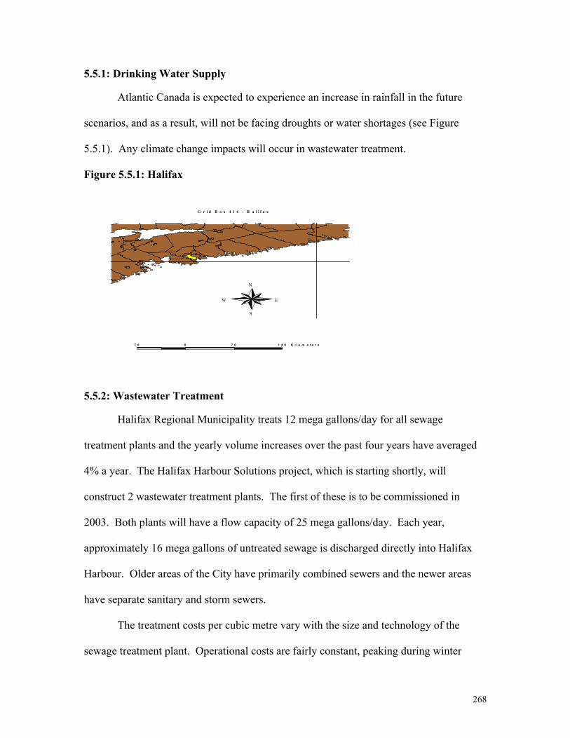
268

5.5.1: Drinking Water Supply

Atlantic Canada is expected to experience an increase in rainfall in the future

scenarios, and as a result, will not be facing droughts or water shortages (see Figure

5.5.1). Any climate change impacts will occur in wastewater treatment.

Figure 5.5.1: Halifax

5.5.2: Wastewater Treatment

Halifax Regional Municipality treats 12 mega gallons/day for all sewage

treatment plants and the yearly volume increases over the past four years have averaged

4% a year. The Halifax Harbour Solutions project, which is starting shortly, will

construct 2 wastewater treatment plants. The first of these is to be commissioned in

2003. Both plants will have a flow capacity of 25 mega gallons/day. Each year,

approximately 16 mega gallons of untreated sewage is discharged directly into Halifax

Harbour. Older areas of the City have primarily combined sewers and the newer areas

have separate sanitary and storm sewers.

The treatment costs per cubic metre vary with the size and technology of the

sewage treatment plant. Operational costs are fairly constant, peaking during winter

7 0 0 7 0 1 4 0 K i l o m e t e r s

N

EW

S

G r i d B o x 4 1 4 - H a l i f a x

269

months due to additional heating and snow removal. At the largest secondary plant

treatment costs are $0.85 per cubic metre and at the largest primary plant the costs are

$0.06 per cubic metre. Heavy rain periods do impact on treatment plant performance due

to hydraulic peaking, but periods of intense rainfall do not impact costs of sewage

treatment plants as compared to pump stations.

We now consider the possible impact of changing precipitation patterns expected

in the next 100 years based on the CGCM1 model. Table 5.5.1 gives the descriptive

statistics of downscaled precipitation for Halifax.

Table 5.5.1 Descriptive Precipitation Statistics for Halifax 1961-2099 1961-1990 2010-2039 2040-2069 2070-2099 Maximum 1543.68 371.7 1543.68 928.49 1234.04 Minimum 2.42 18 6.65 2.42 5.75 Average 149.3 131.88 155.1 153.55 156.69 Stand. Dev. 120.9 60.51 134.02 131.99 138.33

Table 5.5.1 shows that maximum precipitation increases a dramatic 315% from

the baseline period to the 2020 period. It remains 149% to 232% higher in the

subsequent periods. The standard deviation also increases in the future time periods from

the baseline. It shows a 121%, 118% and 128% increase in the respective time periods.

Average daily flow divided by capacity rating is equal to 48%. The mean

precipitation for 1961 to 1990 is 131mm. A simple calculation will show the

precipitation level in a single month that will force the treatment plants to operate at

100%, which is 273 mm. Therefore, precipitation beyond 273mm a month will cause

storm water to overflow into the ecosystem.

5.5.3: Regression Results for Halifax

As with the other case studies, we now report on regressions on precipitation for

Halifax.

270

The estimated regression for 1961 to 1990 is:

PPT = 166.22 – 31.31D2 –33.56D3 –40.28D4 –49.73D5 –53.9D6 –64.48D7 –54.55D8 (16.19) (-2.15) (-2.31) (-2.77) (-3.42) (-3.71) (-4.44) (-3.75)

–63.71D9 -29.04D10 –3.45D11 +11.99D12 (-4.38) (-2) (-0.23) (0.82)

The estimated regression for 2010-2039 is:

PPT = 202.54 –62.29D2 –31.5D3 –58.62D4 –67.27D5 –76.09D6 –100.34D7 –94.78D8

(8.68) (-1.88) (-0.95) (-1.77) (-2.04) (2.3) (-3.04) (-2.87)

–100.9D9–32.54D10 +61.79D11 –6.72D12 (-3.06) (-0.98) (1.87) (-0.2)

The estimated regression for 2040-2069 is: PPT = 196.58 –42.27D2 –39.62D3 –33.74D4 –63.88D5 –71.96D6 –91.87D7 –94.62D8 (8.46) (-1.28) (-1.2) (-1.02) (-1.94) (-2.19) (-2.79) (-2.88)

–96.73D9 –7.05D10 +44.46D11 –19D12 (-2.94) (-0.21) (1.35) (-0.57)

The estimated regression for 2070 to 2099 is: PPT = 187.83 –9.46D2 –45.88D3 –13.52D4 –58.13D5 –39.24D6 –83.33D7 –101.93D8 (7.75) (-0.27) (-1.33) (-0.39) (-1.69) (-1.14) (-2.43) (-2.97)

–93.77D9 +21D10+49.21D11 +1.37D12 (-2.73) (0.61) (1.43) (0.04)

These regression results, which are graphed in Figures 5.5.2 to 5.5.5, show the

relationship between precipitation and the eleven dummy variables. The constant, which

is also the mean precipitation for January, is higher in the future scenarios than in the

baseline. The constant is significant in each scenario. The regression results and 95%

confidence intervals are plotted in Figures 5.5.2 to 5.5.5.

271

Figure 5.5.2: Results for Halifax (1961-1990) Figure 5.5.3: Results for Halifax (2010-2039)

Halifax 1961-1990

0

50

100

150

200

250

300

JAN FEB MAR APR MAY JUN JUL AUG SEP OCT NOV DECMonths

Prec

ipita

tion

in

mm

Crit ical Precipit at ion Level Lower Mean Upper

Halifax 2010-2039

0

100

200

300

400

JAN FEB MAR APR MAY JUN JUL AUG SEP OCT NOV DECMonths

Prec

ipita

tion

in

mm

Crit ical Precipit at ion Level Lower Mean Upper

272

Figure 5.5.4: Results for Halifax (2040-2069)

Figure 5.5.5: Results for Halifax (2070-2099)

The graphs indicate that Halifax will be facing a wastewater treatment capacity

problem in November of the future scenarios as the upper confidence level exceeds the

maximum capacity. Precipitation decreases in the summer months and then increases in

October and November in the future scenarios.

Halifax 2040-2069

050

100150200250300350

JAN FEB MAR APR MAY JUN JUL AUG SEP OCT NOV DECMonths

Prec

ipita

tion

in

mm

Crit ical Precipit at ion Level Lower Mean Upper

Halifax 2070-2099

0

50

100

150

200

250

300

JAN FEB MAR APR MAY JUN JUL AUG SEP OCT NOV DECMonths

Prec

ipita

tion

in m

m

Crit ical Precipit at ion Level Lower Mean Upper

273

Table 5.5.2: Upper Confidence Level to Exceed Halifax’s Wastewater Capacity

Upper Confidence Level Exceeding

Upper Confidence Level Exceeding

Upper Confidence Level Exceeding

Upper Confidence Level Exceeding

Halifax’s Wastewater

Capacity 1961 to 1990

Halifax’s Wastewater Capacity

2010 to 2039

Halifax’s Wastewater

Capacity 2040 to 2069

Halifax’s Wastewater

Capacity 2070 to 2099

January 0 0 0 0 February 0 0 0 0 March 0 0 0 0 April 0 0 0 0 May 0 0 0 0 June 0 0 0 0 July 0 0 0 0 August 0 0 0 0 September 0 0 0 0 October 0 0 0 9 November 0 36 12 37 December 0 0 0 0 Totals 0 36 12 46

Halifax will be facing a wastewater treatment capacity problem when the upper

confidence level exceeds the maximum treatment capacity. This occurs in November of

every future scenario and in October of the 2080 scenario (see Table 5.5.2).

5.5.4: Costs of Adaptation

The maximum treatment capacity is 273 mm of precipitation and in the 2020

scenario, this is exceeded by 36 mm in November. This means that the treatment plant

would have to expand capacity by 13% to prevent overflows. In order to determine the

costs of adaptation, the capital expenditures and investments in the wastewater system are

required. This is a subject for further research.

In lieu of specific numbers associated with Halifax, we use the estimate of the

costs of new wastewater treatment facilities as described in Section 5.10.2. Assuming

expanding capacity costs $50 million, a conservative estimate of adaptation costs is $6.5

million.

274

5.5.5: Summary and Conclusion

At present, Halifax discharges 16 mega gallons of untreated sewage per day into

the Halifax Harbour. However, new planned treatment capacity will come on stream in

2003. Based on this information and the regression analysis, it appears that Halifax will

experience a wastewater treatment capacity shortfall in the future scenarios. The costs

associated with climate change adaptation will include those that expand treatment

capacity, and a rough estimate of this cost is $6.5 million.

5.6: The Prairies

Although the Prairies are a semi-arid to sub-humid area, Saskatchewan has

excellent natural sources of water, including surface water systems and large

underground aquifers. In the Prairies, most runoff begins as snowmelt each spring.

Groundwater supplies are recharged in the spring by replenishing water in the aquifer.

Groundwater maintains a water flow during dry periods through its gradual discharge to

rivers and streams. From 1998 to 2000, southwest Saskatchewan experienced a below

normal spring runoff, resulting in very little or no stored water in many dugouts and

reservoirs. Only 40% of the population has access to a truly secure supply of water:

those served by the North and South Saskatchewan Rivers and the various dams, canals,

pipelines, pump stations and water works associated with these two river systems

In Saskatchewan, the major withdrawal uses of water are agriculture (75.3%),

residential (8.3%), power (1.9%), industrial (0.4%) and mining (14.1%). The average

Saskatchewan resident uses about 380 litres of water per day. The average shower uses

135 litres, washing dishes by hand 40 litres, washing dishes by machine 55 litres,

washing car 75 litres, daily food and drink 2 litres, flushing the toilet 20 litres and

275

watering the lawn for 30 minutes uses 900 litres ( Sask Water Education Website 2001;

www.saskwater.com/htdocs/educatn/waterall.htm).

Some areas of southwest Saskatchewan, including Assiniboia, Swift Current,

Leader and Val Marie, have received only 40 to 70% of normal precipitation from

November 1 to January 1, 2000. In these same areas, fall soil moisture levels prior to

freeze-up ranged from dry to very dry, and as a result, a significant portion of the

snowmelt will be lost to infiltration before contributing to runoff.

5.6.1: Regina, SK

The City of Regina draws water from the South Saskatchewan River (see Figure

5.6.1). Lake Diefenbaker is 150 km from the river, and there is a reservoir 60 km from

the river called Buffalo Pound Lake. Because of these sources of water, rainfall is

irrelevant for local water supplies. Groundwater provides the strategic water supply, as

Regina has access to an aquifer over 10,000 years old, from which 60,000,000 litres of

water a day can be pumped indefinitely (Source: personal communication with City of

Regina Municipal Engineering Department). The investment in capital assets, which is

comprised of the property, plant and equipment for the City of Regina totals $36,837,079.

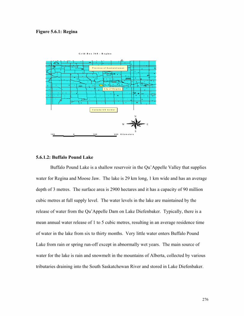
276

Figure 5.6.1: Regina

5.6.1.2: Buffalo Pound Lake

Buffalo Pound Lake is a shallow reservoir in the Qu’Appelle Valley that supplies

water for Regina and Moose Jaw. The lake is 29 km long, 1 km wide and has an average

depth of 3 metres. The surface area is 2900 hectares and it has a capacity of 90 million

cubic metres at full supply level. The water levels in the lake are maintained by the

release of water from the Qu’Appelle Dam on Lake Diefenbaker. Typically, there is a

mean annual water release of 1 to 5 cubic metres, resulting in an average residence time

of water in the lake from six to thirty months. Very little water enters Buffalo Pound

Lake from rain or spring run-off except in abnormally wet years. The main source of

water for the lake is rain and snowmelt in the mountains of Alberta, collected by various

tributaries draining into the South Saskatchewan River and stored in Lake Diefenbaker.

1 0 0 0 1 0 0 2 0 0 K i l o m e t e r s

N

EW

S

G r i d B o x 3 6 8 - R e g i n a

C it y o f R e g i n a

C a n a d a - U S b o r d e r

P r o v i n c e o f S a s k a t c h e w a n

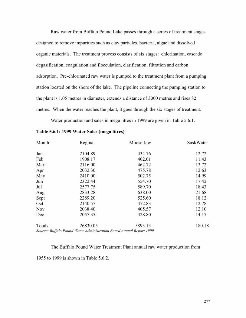
277

Raw water from Buffalo Pound Lake passes through a series of treatment stages

designed to remove impurities such as clay particles, bacteria, algae and dissolved

organic materials. The treatment process consists of six stages: chlorination, cascade

degasification, coagulation and flocculation, clarification, filtration and carbon

adsorption. Pre-chlorinated raw water is pumped to the treatment plant from a pumping

station located on the shore of the lake. The pipeline connecting the pumping station to

the plant is 1.05 metres in diameter, extends a distance of 3000 metres and rises 82

metres. When the water reaches the plant, it goes through the six stages of treatment.

Water production and sales in mega litres in 1999 are given in Table 5.6.1.

Table 5.6.1: 1999 Water Sales (mega litres)

Month Regina Moose Jaw SaskWater

Jan 2104.89 434.76 12.72 Feb 1908.17 402.01 11.43 Mar 2116.00 462.72 13.72 Apr 2032.30 475.78 12.63 May 2410.00 502.75 14.99 Jun 2322.44 554.70 17.42 Jul 2577.75 589.70 18.43 Aug 2833.28 638.00 21.68 Sept 2289.20 525.60 18.12 Oct 2140.57 472.83 12.78 Nov 2038.40 405.57 12.10 Dec 2057.35 428.80 14.17

Totals 26830.05 5893.13 180.18 Source: Buffalo Pound Water Administration Board Annual Report 1999

The Buffalo Pound Water Treatment Plant annual raw water production from

1955 to 1999 is shown in Table 5.6.2.

278

Table 5.6.2: Annual Raw Water Production

Year Raw Water Produced in Megalitres 1955 3500 1960 11500 1965 11500 1970 20000 1975 24000 1980 26000 1985 32500 1990 37000 1999 34000 Source: Buffalo Pound Water Administration Board Annual Report 1999

Annual costs of treatment for the Buffalo Pound Water Treatment Plant for 1999

were $118.15/ML based on a production of 32,903.4ML. The cost of treatment varies

primarily with volume of water produced, though summer treatment also includes

filtering through granular activated carbon to improve taste and odour. Storm events do

have an impact on treatment. As stated before, Buffalo Pound is a shallow lake (6 m

typical depth), which is easily and thoroughly disturbed by storms, which leads to

increased flocculation costs.

5.6.1.3: Operations and Capital Projects

All critical plant equipment at the Buffalo Pound Treatment Plant is inspected,

tested and maintained at least annually to help ensure satisfactory operation during peak

flow demands. Several projects were completed with funds from the Capital

Replacement Reserve for a total cost of $366,535. The control systems and boiler were

replaced in the carbon regeneration plant, and an all-terrain forklift was replaced with a

new four-wheel drive unit. There were also several maintenance projects including: the

installation of new chlorine residual analysers, new chlorine weigh scales at the lake

pumping station, new gas projection heaters were installed in the granular activated

279

carbon contactor area, new steam projection heaters were installed in the clarifier area,

the effluent valves on several carbon contactors were overhauled, and a 1750 HP motor

from the lake pumping station was serviced. The cost of the capital asset additions from

1998 and 1999 are:

LPS Ventilation Intake Filter $3,677 Particle Counters 60,847 Ion Chromatograph 28,829 Regeneration Plant Boiler 41,275 Clarifier Effluent Turbidimeter 14,869 Spectrophotometer 18,709 Source: Buffalo Pound Water Administration Board Annual Board 1999

The combined property, plant and equipment and work in progress capital

expenditures from the Capital Replacement Reserve fund in 1999 totalled $366,535. In

1998, the figure was $228,814.

The total operations and maintenance expenditures equal $5,028,462. The

proportion of the operations and maintenance budget that is spent on equipment

maintenance is 11.35%. Some of these items are:

Pumping Station Equipment Maintenance $48,310 Raw Water Pipe Maintenance 26,168 Building Maintenance 52,217 Electrical Maintenance 19,194 Plant Equipment Maintenance 282,233 Source: Buffalo Pound Water Administration Board Annual Report 1999

5.6.2: Drinking Water Supply

Regina’s primary source of water supply is Buffalo Pound Lake, which has a

production capacity of 150 ML/day. The water is treated and delivered to Regina from

280

the Buffalo Pound Water Treatment Plant, a facility that is jointly owned by the Cities of

Regina and Moose Jaw. It has a peak capacity of 205 ML/day. The secondary source

comes from the many large wells that are located around the city with a production

capacity of 62 ML/day. The water from these wells is used mainly in the summer months

when there is high water demand. During these periods, the water from both sources is

mixed together in large reservoirs, to ensure consistent water quality. Water delivered

from the Buffalo Pound Water Treatment Plant passes through a 57 km long, 900mm (36

inch) diameter steel pipeline. There is a second larger pipeline being constructed,

scheduled for completion in 2003. The purpose of this pipeline is to ensure supply

security in the event of problems in the original pipeline, to increase the maximum

amount of water the plant can deliver to the City, and to eliminate the need to supplement

Buffalo Pound water supply with well water. The lake intake and the raw water pipeline

from the lake pumping station is to be twinned, along with the replacement of the fish

screen. In October 2000, the Buffalo Pound Lake control structure and dam enhancement

project was officially opened. The project was initiated in order to sustain the long-term

viability of the water supply. The 1,100 cubic metres of concrete, 85,000 kilograms of

steel, 50,000 cubic metres of excavation and 20,000 cubic metres of new embankment

cost $3 million to complete.

The City differentiates between two types of pipeline: supply and distribution.

There are 155.2km of supply pipeline and 792.3km of distribution pipeline. Supply

pipeline connects sources of supply with reservoirs and pumping stations and distribution

piping accounts for all pipes between the pumping station and the customer. The pipes

range in size from 100mm (4 inch) to 1050mm (42 inch). There are three water-pumping

281

stations located within the City limits. There are five treated water storage reservoirs

situated around the city that hold 160 million litres of water. These reservoirs are used to

maintain water supply during times of high demand, to provide water supply during a

power failure or other emergencies, and to provide additional water for fire fighting.

There are three pumping stations to pressurize and deliver water through the water mains

and they can deliver water continuously, even during power failures.

The peak demand per day is 150,000,000 litres. Water is priced on a full cost

recovery basis, at a rate of $0.75 per cubic metre. All water is used for domestic

consumption and light industry; none is used for irrigation. The monthly drinking water

production for the year 2000 is shown in Table 5.6.3.

Table 5.6.3: Monthly Drinking Water Production, 2000

Month Potable Water Production (ML) Jan 2,050 Feb 1,924 Mar 2,056 Apr 2,028 May 2,411 Jun 2,285 Jul 2,595 Aug 2,721 Sep 2,266 Oct 2,259 Nov 2,082 Dec 2,049 Total 26,726 Source: City of Regina Municipal Engineering Department

Regina’s annual water losses are 8% of the total volume of water produced.

Water conservation initiatives over the past decade have resulted in large decreases in

water consumption. Per capita water use has since levelled off and water demand is

282

currently constant, if not slightly decreasing. The population of the City is currently

189,400 people and is growing in the range of 1.5% to 2% per annum. The per capita

consumption of water is 386.6 litres/day/capita. This figure includes all uses of water,

residential, commercial, recreational and losses.

5.6.3: Wastewater Treatment

The annual costs for treatment for the City of Regina Wastewater Treatment Plant

are:

Treatment cost/volume treated $147.21/ML Treatment cost/tonnes of contaminants removed $250.32/tonne Treatment cost/capita $20.08/person Source: City of Regina Municipal Engineering Department

The City of Regina has 725 km of sewers and 15 lift stations that collect domestic

sewage across the City. The wastewater is treated at the sewage treatment facilities using

a UV radiation treatment rendering it a better quality than the water in Buffalo Pound

Lake. There are about 80 million litres of sewage moving through the system each day.

The treated water is then discharged into the Qu’Appelle system. Storm runoff is

collected by approximately 850km of underground storm sewers that drain into the north

and south channels and Wascana Creek.

Table 5.6.4 show the descriptive statistics for precipitation for the four time

periods.

Table 5.6.4: Precipitation Descriptive Statistics for Regina 1961-2099 1961-1990 2010-2039 2040-2069 2070-2099 Maximum 895.85 211.5 770.44 895.85 842.8 Minimum 0.69 0.9 0.69 0.78 1.11 Average 48.31 38.09 49.66 52.14 53.35 Stand. Dev. 64.87 29.75 69.34 70.68 77.67

283

A comparison of the mean values for the baseline and four scenarios, 2020, 2050

and 2080 show that the average precipitation will increase over this time period by 40%

by the 2080 scenario from the baseline. The standard deviation increases by 133% from

the baseline period to the 2020 scenario. The standard deviation continues to increase

over the next two periods.

5.6.4: Regression Results

In order to consider changes in the pattern of precipitation due to climate change,

we carried out some regressions, just as we did with the other case studies.

The estimated regression for 1961 to 1990 is as follows:

PPT= 27.4 – 3.8D2 – 0.12D3 – 0.07D4 + 29.14D5 + 44.55D6 + 36.39D7 + 16.86D8 + (5.97) (-0.58) (-0.01) (-0.01) (4.49) (6.87) (5.61) (2.6)

11.47D9 –1.38D10 – 7.16D11 + 2.39D12 (1.76) (-0.21) (-1.1) (0.369)

The estimated regression for 2010 to 2039 is:

PPT= 30.77 + 0.96D2 + 1.7D3 + 4.9D4 + 40.74D5 + 72.55D6 + 63.21D7 + 22.51D8 + (2.57) (.057) (.101) (0.29) (2.41) (4.29) (3.74) (1.33)

26.36D9 – 0.21D10 – 2.75D11 – 3.24D12 (1.56) (-0.01) (-0.16) (-0.19) The estimated regression for 2040 to 2069 is:

PPT= 27.89 + 4.04D2 + 9.87D3 + 24.32D4 + 50.58D5 + 57.11D6 + 37.86D7 + 60.6D8 (2.24) (0.23) (0.56) (1.38) (2.88) (3.25) (2.15) (3.45)

+ 38.08D9 + 9.06D10 – 3.2D11 + 2.6D12 (2.16) (0.51) (-0.18) (0.14) The estimated regression for 2070 to 2099 is:

PPT= 28.26 + 7.99D2 + 17.21D3 + 19.21D4 + 53.06D5 + 47.91D6 + 65.08D7 + (2.05) (0.41) (0.88) (0.98) (2.72) (2.45) (3.33)

54.49D8 + 19.64D9 +10.24D10 – 1.82D11 + 7.99D12 (2.79) (1) (0.52) (-0.09) (0.41)

284

The results of the above regressions are plotted in Figures 5.6.2 to 5.6.5. The

regressions give the mean precipitation and 95% confidence interval.

Figure 5.6.2: Results for Regina (1961—1990) Figure 5.6.3: Results for Regina (2010-2039)

Regina 1961-1990

0

20

40

60

80

100

JAN FEB MAR APR MAY JUN JUL AUG SEP OCT NOV DEC

Months

Prec

ipita

tion i

n mm

Lower Mean Upper

Regina 2010-2039

020406080

100120140

JAN FEB MAR APR MAY JUN JUL AUG SEP OCT NOV DECMonths

Prec

ipita

tion

in m

m

Lower Mean Upper

285

Figure 5.6.4: Results for Regina (2040-2069) Figure 5.6.5: Results for Regina (2070-2099)

The graphs indicate that precipitation will increase in the future scenarios in the

summer months and that water supply will not be severely depleted. In the 2050

scenario, precipitation decreases dramatically in July.

5.6.5: Summary and Conclusion

Regina 2040-2069

0

50

100

150

JAN FEB MAR APR MAY JUN JUL AUG SEP OCT NOV DEC

Months

Prec

ipita

tion

in

mm

Lower Mean Upper

Regina 2070-2099

-50

0

50

100

150

JAN FEB MAR APR MAY JUN JUL AUG SEP OCT NOV DEC

Months

Prec

ipita

tion

in

mm

Lower Mean Upper

286

The City of Regina would incur adaptation costs if the South Saskatchewan River

were seriously depleted or the aquifer were to dry up. On the basis of local expert

opinion, there does not appear to be either a water supply or wastewater treatment

problem. However, a further study must be done on a watershed basis to determine if

climate change will adversely affect water flows in the South Saskatchewan River (see

Section 5.14).

5.7: Humboldt, SK

The Wakaw-Humboldt area has long suffered from serious water shortages, as

groundwater supplies can be shallow even in times of normal runoff (see Figure 5.7.1).

Local surface supplies are difficult to treat because of high organic content, and the deep

groundwater sources are highly mineralized and expensive to treat. Well maintenance is

also expensive. Because of these issues, Sask Water built a regional water supply

system. The area now uses water from the South Saskatchewan River, and the system

distributes water to 10 000 people in nine communities and eight rural municipalities.

These communities are Hoey, St. Isidore-de-Bellevue, Domremy, Wakaw, Bruno,

Humboldt, Muenster, Annaheim and Lake Lenore. These rural municipalities get their

water from the North Central Rural Pipeline Association, and the SHL Rural Pipeline

Association. The system consists of a pump station on the South Saskatchewan River,

two booster pump stations, a water treatment plant at Wakaw and 190 kms of pipeline.

The total cost of the system was $32.3 million, of which $2.8 million was contributed by

the Canada-Saskatchewan Infrastructure Works Program; $3.8 million by the federal-

provincial Partnership Agreement on Water-Based Economic Development (PAWBED).

287

The remaining $25.7 million is being financed by Sask Water and will be recovered over

a 30 year period through charges to water users.

Figure 5.7.1: Humboldt

5.7.1: Drinking Water Supply and Sask Water

Sask Water is Saskatchewan’s water manager and is mandated to provide quality

water to rural Saskatchewan residents including those living in Humboldt and Melfort.

The utility operations of Sask Water include 135 km of canal, 5 reservoirs, 32

pumping facilities and 4 water treatment plants. There are 725 km of pipeline ranging in

diameter from 76mm to 750mm. The utility supplies both treated and raw water to

industrial, municipal and domestic customers. The rural municipal population served by

Sask Water is approximately 38,000 customers. In 2000, the total consumption of raw

water was 168,716,436 gallons, and for treated water, this figure was 730,957,427

gallons.

1 0 0 0 1 0 0 2 0 0 K i l o m e t e r s

N

EW

S

G r i d B o x 3 3 3 - H u m b o l d t

T o w n o f H u m b o l d t

P r o v i n c e o f S a s k a t c h e w a n

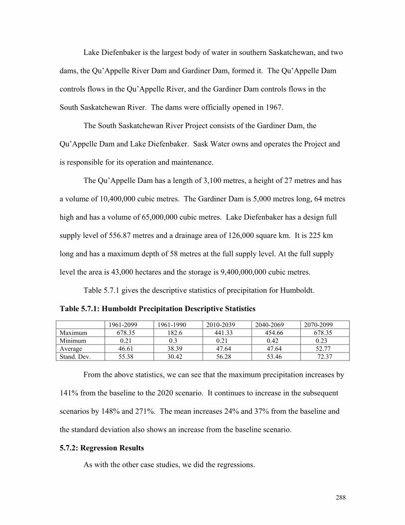
288

Lake Diefenbaker is the largest body of water in southern Saskatchewan, and two

dams, the Qu’Appelle River Dam and Gardiner Dam, formed it. The Qu’Appelle Dam

controls flows in the Qu’Appelle River, and the Gardiner Dam controls flows in the

South Saskatchewan River. The dams were officially opened in 1967.

The South Saskatchewan River Project consists of the Gardiner Dam, the

Qu’Appelle Dam and Lake Diefenbaker. Sask Water owns and operates the Project and

is responsible for its operation and maintenance.

The Qu’Appelle Dam has a length of 3,100 metres, a height of 27 metres and has

a volume of 10,400,000 cubic metres. The Gardiner Dam is 5,000 metres long, 64 metres

high and has a volume of 65,000,000 cubic metres. Lake Diefenbaker has a design full

supply level of 556.87 metres and a drainage area of 126,000 square km. It is 225 km

long and has a maximum depth of 58 metres at the full supply level. At the full supply

level the area is 43,000 hectares and the storage is 9,400,000,000 cubic metres.

Table 5.7.1 gives the descriptive statistics of precipitation for Humboldt.

Table 5.7.1: Humboldt Precipitation Descriptive Statistics 1961-2099 1961-1990 2010-2039 2040-2069 2070-2099 Maximum 678.35 182.6 441.33 454.66 678.35 Minimum 0.21 0.3 0.21 0.42 0.23 Average 46.61 38.39 47.64 47.64 52.77 Stand. Dev. 55.38 30.42 56.28 53.46 72.37

From the above statistics, we can see that the maximum precipitation increases by

141% from the baseline to the 2020 scenario. It continues to increase in the subsequent

scenarios by 148% and 271%. The mean increases 24% and 37% from the baseline and

the standard deviation also shows an increase from the baseline scenario.

5.7.2: Regression Results

As with the other case studies, we did the regressions.

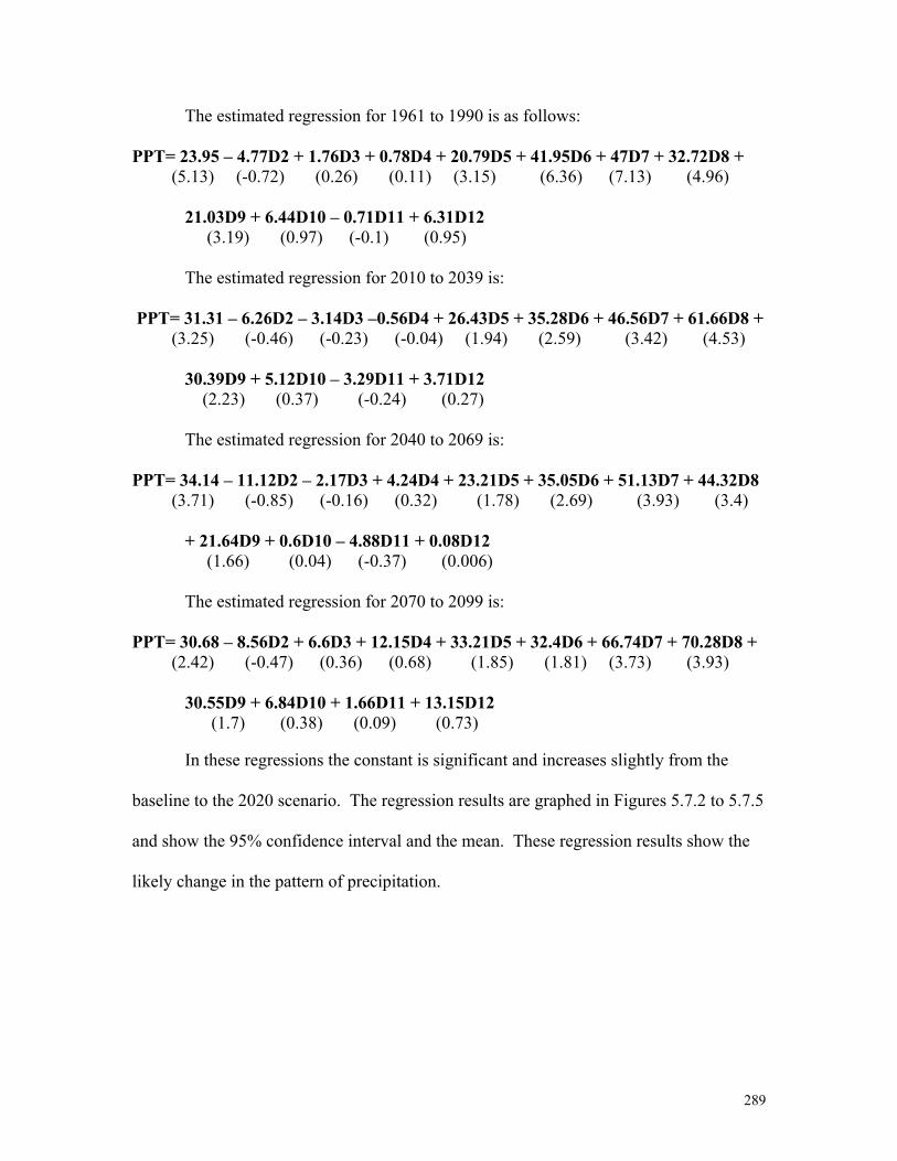
289

The estimated regression for 1961 to 1990 is as follows:

PPT= 23.95 – 4.77D2 + 1.76D3 + 0.78D4 + 20.79D5 + 41.95D6 + 47D7 + 32.72D8 + (5.13) (-0.72) (0.26) (0.11) (3.15) (6.36) (7.13) (4.96)

21.03D9 + 6.44D10 – 0.71D11 + 6.31D12 (3.19) (0.97) (-0.1) (0.95) The estimated regression for 2010 to 2039 is:

PPT= 31.31 – 6.26D2 – 3.14D3 –0.56D4 + 26.43D5 + 35.28D6 + 46.56D7 + 61.66D8 + (3.25) (-0.46) (-0.23) (-0.04) (1.94) (2.59) (3.42) (4.53)

30.39D9 + 5.12D10 – 3.29D11 + 3.71D12 (2.23) (0.37) (-0.24) (0.27)

The estimated regression for 2040 to 2069 is:

PPT= 34.14 – 11.12D2 – 2.17D3 + 4.24D4 + 23.21D5 + 35.05D6 + 51.13D7 + 44.32D8 (3.71) (-0.85) (-0.16) (0.32) (1.78) (2.69) (3.93) (3.4)

+ 21.64D9 + 0.6D10 – 4.88D11 + 0.08D12 (1.66) (0.04) (-0.37) (0.006) The estimated regression for 2070 to 2099 is:

PPT= 30.68 – 8.56D2 + 6.6D3 + 12.15D4 + 33.21D5 + 32.4D6 + 66.74D7 + 70.28D8 + (2.42) (-0.47) (0.36) (0.68) (1.85) (1.81) (3.73) (3.93)

30.55D9 + 6.84D10 + 1.66D11 + 13.15D12 (1.7) (0.38) (0.09) (0.73)

In these regressions the constant is significant and increases slightly from the

baseline to the 2020 scenario. The regression results are graphed in Figures 5.7.2 to 5.7.5

and show the 95% confidence interval and the mean. These regression results show the

likely change in the pattern of precipitation.

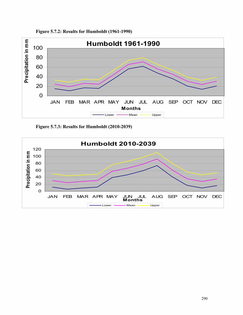
290

Figure 5.7.2: Results for Humboldt (1961-1990)

Figure 5.7.3: Results for Humboldt (2010-2039)

Humboldt 1961-1990

0

20

40

60

80

100

JAN FEB MAR APR MAY JUN JUL AUG SEP OCT NOV DECMonths

Prec

ipita

tion

in m

m

Lower Mean Upper

Humboldt 2010-2039

0

20

40

60

80

100

120

JAN FEB MAR APR MAY JUN JUL AUG SEP OCT NOV DECMonths

Prec

ipitat

ion in

mm

Lower Mean Upper

291

Figure 5.7.4: Results for Humboldt (2040-2069)

Figure 5.7.5: Results for Humboldt (2070-2099)

The graphs indicate that the upper confidence interval is increasing over the four

scenarios as well as the mean. We can see that precipitation peaks in July and August

and is at its lowest in February and November.

Humboldt 2070-2099

-50

0

50

100

150

JAN FEB MAR APR MAY JUN JUL AUG SEP OCT NOV DEC

Months

Prec

ipita

tion

in m

m

Lower Mean Upper

H u m b o ld t 2 0 4 0 -2 0 6 9

02 04 06 08 0

1 0 01 2 0

JA N FEB MA R A PR MA Y JUN JUL A UG SEP OCT NOV DECM onths

Pre

cipi

tatio

n in

mm

L o w e r M e a n U p p e r

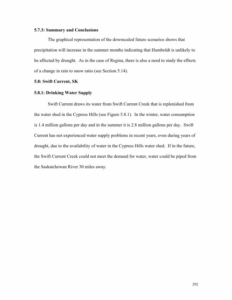
292

5.7.3: Summary and Conclusions

The graphical representation of the downscaled future scenarios shows that

precipitation will increase in the summer months indicating that Humboldt is unlikely to

be affected by drought. As in the case of Regina, there is also a need to study the effects

of a change in rain to snow ratio (see Section 5.14).

5.8: Swift Current, SK 5.8.1: Drinking Water Supply

Swift Current draws its water from Swift Current Creek that is replenished from

the water shed in the Cypress Hills (see Figure 5.8.1). In the winter, water consumption

is 1.4 million gallons per day and in the summer it is 2.8 million gallons per day. Swift

Current has not experienced water supply problems in recent years, even during years of

drought, due to the availability of water in the Cypress Hills water shed. If in the future,

the Swift Current Creek could not meet the demand for water, water could be piped from

the Saskatchewan River 30 miles away.

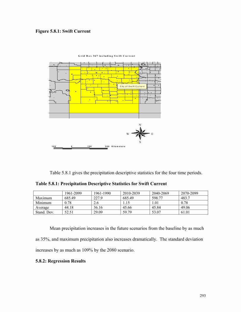
293

Figure 5.8.1: Swift Current

Table 5.8.1 gives the precipitation descriptive statistics for the four time periods.

Table 5.8.1: Precipitation Descriptive Statistics for Swift Current 1961-2099 1961-1990 2010-2039 2040-2069 2070-2099 Maximum 685.49 227.9 685.49 598.77 483.7 Minimum 0.78 2.6 1.15 1.01 0.78 Average 44.18 36.16 45.66 45.84 49.06 Stand. Dev. 52.51 29.09 59.79 53.07 61.01

Mean precipitation increases in the future scenarios from the baseline by as much

as 35%, and maximum precipitation also increases dramatically. The standard deviation

increases by as much as 109% by the 2080 scenario.

5.8.2: Regression Results

1 0 0 0 1 0 0 2 0 0 K i l o m e t e r s

N

EW

S

G r i d B o x 3 6 7 i n c l u d i n g S w i f t C u r r e n t

C it y o f S w i f t C u r re n t

294

The following regressions consider the likely change in the pattern of precipitation for

Swift Current.

The estimated regression for 1961 to 1990 is as follows:

PPT= 27.6 – 5.38D2 – 0.33D3 +2.61D4 + 23.48D5 + 44.53D6 + 25.43D7 + 13.8D8 + (5.99) (-0.82) (-0.05) (0.4) (3.6) (6.83) (3.9) (2.11)

10.62D9 – 6.23D10 – 7.65D11 + 1.78D12 (1.63) (-0.95) (-1.17) (0.27)

The estimated regression for 2010 to 2039 is:

PPT= 31.64 – 5.56D2 + 3.68D3 + 3.59D4 + 27.22D5 + 70.33D6 + 40.37D7 + 7.58D8 + (3.07) (-0.38) (0.25) (0.24) (1.87) (4.83) (2.77) (0.52)

30.42D9 – 2.1D10 – 4.66D11 – 2.71D12 (2.09) (-0.14) (-0.32) (-0.18)

The estimated regression for 2040 to 2069 is:

PPT= 30.36 – 5.82D2 + 7.91D3 + 17.81D4 + 37.2D5 + 45.9D6 + 27.03D7 + 33.03D8 + (3.28) (-0.44) (0.6) (1.36) (2.84) (3.5) (2.06) (2.52)

31.79D9 - 1.67D10 – 7.76D11 + 0.33D12 (2.42) (-0.12) (-0.59) (0.02) The estimated regression for 2070 to 2099 is:

PPT= 33.61 – 5.45D2 + 9.43D3 + 16.25D4 + 33.38D5 + 58.77D6 + 43.47D7 + 15.35D8 (3.14) (-0.36) (0.62) (1.07) (2.2) (3.88) (2.87) (1.01)

+ 20.43D9 - 1.58D10 – 6.11D11 + 1.51D12 (1.34) (-0.1) (-0.4) (0.09)

These regression results show the likely pattern of precipitation in the future

scenarios. The constant is significant in each scenario but only increases slightly from

the baseline. The 95% confidence intervals are graphed in Figures 5.8.2 to 5.8.5.

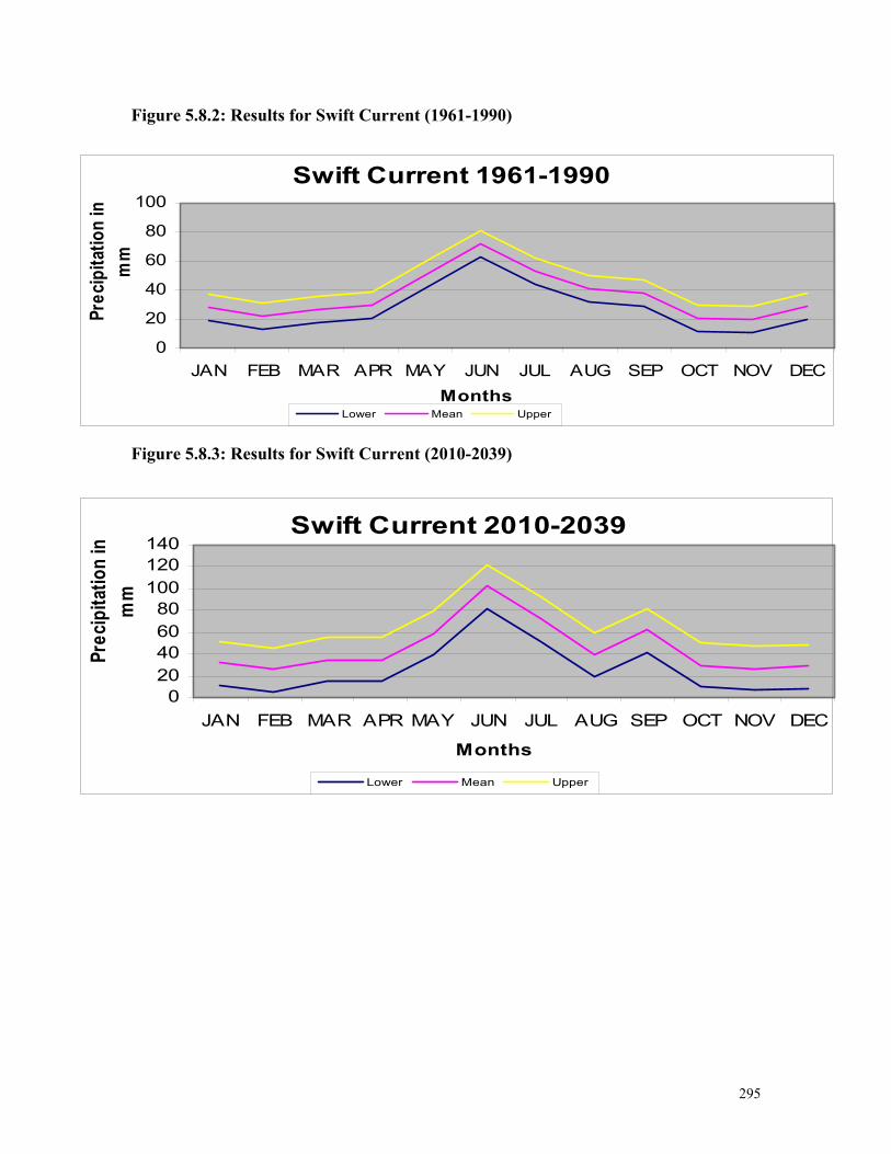
295

Figure 5.8.2: Results for Swift Current (1961-1990) Figure 5.8.3: Results for Swift Current (2010-2039)

Swift Current 1961-1990

0

20

40

60

80

100

JAN FEB MAR APR MAY JUN JUL AUG SEP OCT NOV DECMonths

Prec

ipita

tion

in

mm

Lower Mean Upper

Swift Current 2010-2039

020406080

100120140

JAN FEB MAR APR MAY JUN JUL AUG SEP OCT NOV DEC

Months

Prec

ipita

tion

in

mm

Lower Mean Upper

296

Figure 5.8.4: Results for Swift Current (2040-2069) Figure 5.8.5: Results for Swift Current (2070-2099)

In the 2050 scenario, precipitation is projected to decrease in July and increase in

August and September to the June level. In the 2080 scenario, it decreases in July and

August and increases slightly in September. In the 2020 scenario, precipitation also

decreases dramatically in August. The pattern of precipitation indicates that the late

summers will be dry in the future scenarios.

Swift Current 2040-2069

0

20

40

60

80

100

JAN FEB MAR APR MAY JUN JUL AUG SEP OCT NOV DEC

Months

Prec

ipita

tion

in m

m

Lower Mean Upper

Swift Current 2070-2099

020406080

100120

JAN FEB MAR APR MAY JUN JUL AUG SEP OCT NOV DEC

Months

Prec

ipita

tion

in m

m

Lower Mean Upper

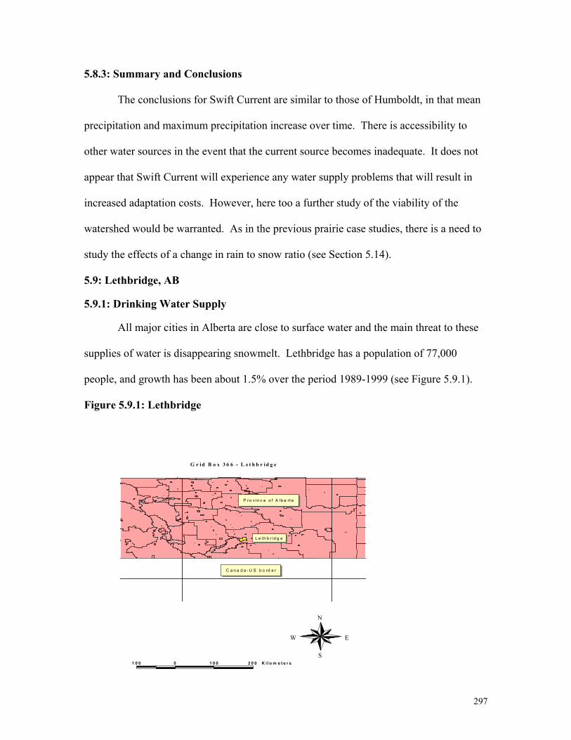
297

5.8.3: Summary and Conclusions

The conclusions for Swift Current are similar to those of Humboldt, in that mean

precipitation and maximum precipitation increase over time. There is accessibility to

other water sources in the event that the current source becomes inadequate. It does not

appear that Swift Current will experience any water supply problems that will result in

increased adaptation costs. However, here too a further study of the viability of the

watershed would be warranted. As in the previous prairie case studies, there is a need to

study the effects of a change in rain to snow ratio (see Section 5.14).

5.9: Lethbridge, AB 5.9.1: Drinking Water Supply

All major cities in Alberta are close to surface water and the main threat to these

supplies of water is disappearing snowmelt. Lethbridge has a population of 77,000

people, and growth has been about 1.5% over the period 1989-1999 (see Figure 5.9.1).

Figure 5.9.1: Lethbridge

1 0 0 0 1 0 0 2 0 0 K i l o m e t e r s

N

EW

S

G r i d B o x 3 6 6 - L e t h b r i d g e

L e t h b r id g e

P ro v in c e o f A lb e rt a

C a n a d a - U S b o rd e r

298

Table 5.9.1 gives the ten-year average water production by month for Lethbridge.

Table 5.9.1: Ten Year Average Water Production in Millions of Litres (ML)

January 984.0 February 932.7 March 1036.0 April 1099.2 May 1478.2 June 1587.6 July 1880.4 August 1931.0 September 1457.7 October 1101.3 November 971.5 December 1011.0

Total 15,470.6 ML Source: Personal Communication from Doug Kaupp, Lethbridge WaterUtilities Manager

The demand for water is within 10% of the production values. The average day

demand is about 42.4 ML/day and peak day demand is about 102 ML/day. Production

capacity is 150 ML/day.

The average demand for water is increasing at about 2% per annum. Peak

demand per capita is decreasing. The water works system includes 4 storage reservoirs

and each has a pump station. The total treated water storage capacity is 77 ML. The

system is comprised of 425 km of distribution pipes.

The average price of water is $0.43 per cubic metre, with the commercial average

at $0.38 per cubic metre. Because the pricing is structured on a full cost recovery basis,

the water utility is able to contribute 8% of revenues to the city in lieu of taxes.

The City of Lethbridge has not imposed bans on water use and no formal

conservation programs are in place. Normal rainfall is 262mm per annum and there is

160 cm of annual snowfall.

299

The source of water is the Oldman River within the South Saskatchewan Basin.

The Oldman River runs through the City and flows into the Bow River, and the Bow

flows into the South Saskatchewan River. Upstream of Lethbridge is the Oldman River

Dam with a reservoir capacity of about 500,000,000 cubic meters. The water release is

controlled by the province to the benefit of large irrigation districts and in stream

requirements, including those determined by inter-provincial flow through agreements.

Water is distributed to users on a first come, first serve, licensing basis.

Repeated drought is of concern; however no supply strategies are in place. A

weir was built forty years ago to guard against low summer flows. Another dam was

built in 1990, and before it was completed, 50% of volume of water flow occurred in

May, June and July. The security of the water supply depends upon the snow pack.

Recently, three consecutive dry years have caused severe problems.

5.9.2: Wastewater Treatment

Lethbridge has state-of-the-art wastewater treatment; biological nutrient removal

(BNR) and UV disinfection removes phosphorus and nitrogen. Average daily flow

received at the treatment plant is 35,000 cubic metres per day, and the plant has a

capacity of 80,000 cubic metres per day. The treated water is discharged further

downstream and the sludge is used on farms. More thunderstorms and concentrated

rainfall could result in infiltration problems. Generally, infiltration does not result in

untreated discharges, and no untreated water is dumped into the river.

Table 5.9.2 shows the descriptive statistics of actual and projected precipitation for

Lethbridge.

300

Table 5.9.2: Descriptive Precipitation Statistics for Lethbridge 1961-2099 1961-1990 2010-2039 2040-2069 2070-2099 Maximum 585.28 183.5 335.92 430.46 585.28 Minimum 0.18 0.5 0.18 0.19 0.26 Average 41.85 36.4 41.45 42.33 47.24 Stand. Dev. 45.76 29.5 44.9 47.58 56.42

The maximum precipitation increases 83% from the baseline to the 2020 time

period. In the subsequent time periods the maximum remains 134% and 218% above the

baseline level, respectively. The mean increases slightly over the four scenarios. The

standard deviation increases 52%, 61% and 91% from the baseline in the subsequent

periods.

On any given day, because daily flow is 35,000 m3, and capacity is 80,000 m3,

43% of the plant capacity is utilized. In the baseline period, the mean precipitation was

36mm. A simple calculation shows that if precipitation exceeded 83mm in a given

month, then untreated wastewater would be discharged.

5.9.3: Regression Results

The estimated regression for 1960 to 1991 is: PPT= 29.13 – 11.54D2 + 1D3 + 9.67D4 + 22.34D5 + 39.61D6 + 13.52D7 + 18.72D8 + (6.17) (-1.73) (0.15) (1.45) (3.35) (5.94) (2.02) (2.8)

16.41D9 – 11.55D10 – 8.85D11 –2.11D12 (2.46) (-1.73) (-1.32) (-0.31)

The estimated regression for 2010 to 2039 is:

PPT= 32.53 – 14.87D2 + 1.14D3 + 10.81D4 + 27.28D5 + 48.85D6 + 12.05D7 + (4.27) (-1.38) (0.1) (1) (2.53) (4.53) (1.11)

23.13D8 + 22.58D9 – 14.24D10 – 3.77D11 –6.01D12 (2.14) (2.09) (-1.32) (-0.35) (-0.55)

The estimated regression for 2040 to 2069 is:

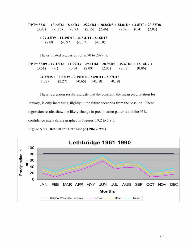
301

PPT= 32.61 – 13.66D2 + 8.66D3 + 25.26D4 + 28.86D5 + 34.81D6 + 4.8D7 + 23.82D8 (3.93) (-1.16) (0.73) (2.15) (2.46) (2.96) (0.4) (2.03)

+ 24.43D9 – 11.39D10 – 6.73D11 –2.16D12 (2.08) (-0.97) (-0.57) (-0.18)

The estimated regression for 2070 to 2099 is: PPT= 35.09 – 14.15D2 + 11.99D3 + 29.61D4 + 28.96D5 + 35.47D6 + 12.14D7 + (3.51) (-1) (0.84) (2.09) (2.05) (2.51) (0.86)

24.37D8 + 32.07D9 – 9.19D10 – 2.69D11 –2.77D12 (1.72) (2.27) (-0.65) (-0.19) (-0.19)

These regression results indicate that the constant, the mean precipitation for

January, is only increasing slightly in the future scenarios from the baseline. These

regression results show the likely change in precipitation patterns and the 95%

confidence intervals are graphed in Figures 5.9.2 to 5.9.5.

Figure 5.9.2: Results for Lethbridge (1961-1990)

Lethbridge 1961-1990

0

20

40

60

80

100

JAN FEB MAR APR MAY JUN JUL AUG SEP OCT NOV DEC

Months

Prec

ipita

tion

in

mm

Crit ical Precipit at ion Level Lower Mean Upper

302

Figure 5.9.3: Results for Lethbridge (2010-2039) Figure 5.9.4: Results for Lethbridge (2040-2069)

Lethbridge 2010-2039

020406080

100120

JAN FEB MAR APR MAY JUN JUL AUG SEP OCT NOV DECMonths

Prec

ipita

tion

in

mm

Crit ical Precipit at ion Level Lower Mean Upper

Lethbridge 2040-2069

0

20

40

60

80

100

JAN FEB MAR APR MAY JUN JUL AUG SEP OCT NOV DECMonths

Prec

ipita

tion

in

mm

Crit ical Precipit at ion Level Lower Mean Upper

303

Figure 5.9.5: Results for Lethbridge (2070-2099)

The graphs show that neither the mean nor the upper confidence interval exceeds

the maximum wastewater treatment capacity in the baseline. However, in the future

scenarios, upper confidence interval of precipitation exceeds the capacity in several

different months.

Table 5.9.3: Upper Confidence Level Exceeding Lethbridge’s Present Wastewater Capacity

Upper C.I Exceeding Upper C.I. Exceeding Upper C.I. Exceeding

Upper C.I. Exceeding

Lethbridge’s Wastewater

Capacity 1961 to 1990

Lethbridge’s Wastewater

Capacity 2010 to 2039

Lethbridge’s Wastewater

Capacity 2040 to 2069

Lethbridge’s Wastewater

Capacity 2070 to 2099

January 0 0 0 0 February 0 0 0 0 March 0 0 0 0 April 0 0 0 1.34 May 0 0 0 0.69 June 0 13.36 0.73 7.2 July 0 0 0 0 August 0 0 0 0 September 0 0 0 3.81 October 0 0 0 0 November 0 0 0 0 December 0 0 0 0 Totals 0 13.36 0.73 13.04

Lethbridge 2070-2099

0

20

40

60

80

100

JAN FEB MAR APR MAY JUN JUL AUG SEP OCT NOV DEC

Months

Prec

ipita

tion

in m

m

Crit ical Precipit at ion Level Lower Mean Upper

304

5.9.4: Costs of Adaptation

In Table 5.9.3, precipitation exceeds the maximum treatment capacity of 83mm

by 13.36mm. This means that capacity would have to expand by 16% to prevent

overflow. In order to determine the costs of adaptation, the amount of capital investment

in the wastewater treatment facilities is required. This is a subject for future research. In

lieu of specific costs for Lethbridge, we can use an estimate of expanding treatment

facilities of $50 million (see Section 5.10.2). Based on this, a rough approximation of the

costs of adaptation to climate change is $8 million.

5.9.5: Summary and Conclusions

As can be seen from Table 5.9.3 precipitation will exceed wastewater treatment

capacity in June of the 2020, 2050 and 2080 scenario and in April, May and September of

the 2080 scenario, indicating that Lethbridge will have to increase its capacity to deal

with effects of climate change. However, the projected increases in precipitation are

small. As with all the prairie case studies, the viability of water supply should be

investigated at the watershed level. In particular, Lethbridge could be vulnerable to

changes in snowpack (see Section 5.14).

5.10: Prince George, BC 5.10.1: Drinking Water Supply

Prince George is a city of 80,000 people located at the confluence of the Fraser

and Nechako Rivers in central British Columbia (see Figure 5.10.1). Although the city

has access to two rivers, it draws its water from 8 producing wells. The pulp and paper

industry discharges huge amounts of pollutants into the Fraser River. There does not

appear to be a water supply problem as the recharge rate is greater than the draw down

rate. The demand for water is unchanged, with some water restrictions in the summer,

305

due to the lack of pumping capacity. Residents pay a flat rate of $13.95/month for water

and $14 for sewage. Overall water production capacity is in excess of 50 gallons per day.

The 8 wells are part of a system consisting of pump stations, 20 booster stations and 400

km of water main line. Water consumption is 513 litres per capita per day. In 2000,

water production is shown in Table 5.10.1.

Figure 5.10.1: Prince George

2 0 0 0 2 0 0 4 0 0 K i l o m e t e r s

N

EW

S

G r id B o x 3 2 8 - P r i n c e G e o r g e

P ro v in c e o f B r i ti s h C o lu m b ia

P rin c e G e o r g e

306

Table 5.10.1: Monthly Water Production 2000

Month Monthly Total (litres) Jan 1,098,009,822 Feb 1,084,015,774 Mar 1,156,172,451 Apr 921,447,987.6 May 1,485,575,281 Jun 1,500,986,414 Jul 1,452,084,875 Aug 1,544,515,268 Sep 1,217,727,050 Oct 1,226,041,843 Nov 1,167,031,710 Dec 1,140,858,808 Total 14,994,467,284 Avg. Daily 41,080,733.08

5.10.2: Wastewater Treatment

Wastewater is treated at the primary and secondary levels, and the secondary

treatment results in water having a biological oxygen demand and suspended solids of 20

milligrams/litre. All sanitary sewers are separate from storm sewers and the storm water

is discharged untreated into the Fraser River. The maximum capacity of the wastewater

treatment plant is 15 million gallons a day or 68.1 million litres per day. Wastewater

treatment costs are $1.1 million per year. Provincial legislation is pending that will

require treatment of storm water before it is discharged. This will require separate

treatment facilities at a cost of $10 to $50 million.

The 2000 wastewater flows in Prince George are shown in Table 5.10.2.

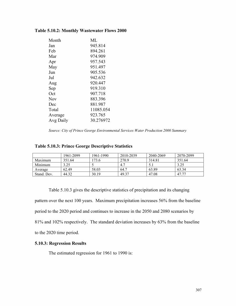
307

Table 5.10.2: Monthly Wastewater Flows 2000

Month ML Jan 945.814 Feb 894.261 Mar 974.909 Apr 957.543 May 951.497 Jun 905.536 Jul 942.632 Aug 920.447 Sep 919.310 Oct 907.718 Nov 883.396 Dec 881.987 Total 11085.054 Average 923.765 Avg Daily 30.276972 Source: City of Prince George Environmental Services Water Production 2000 Summary

Table 5.10.3: Prince George Descriptive Statistics 1961-2099 1961-1990 2010-2039 2040-2069 2070-2099 Maximum 351.64 173.6 270.9 314.81 351.64 Minimum 3.25 5 4.7 5.1 3.25 Average 62.49 58.03 64.7 63.89 63.34 Stand. Dev. 44.32 30.19 49.37 47.08 47.77

Table 5.10.3 gives the descriptive statistics of precipitation and its changing

pattern over the next 100 years. Maximum precipitation increases 56% from the baseline

period to the 2020 period and continues to increase in the 2050 and 2080 scenarios by

81% and 102% respectively. The standard deviation increases by 63% from the baseline

to the 2020 time period.

5.10.3: Regression Results

The estimated regression for 1961 to 1990 is:

308

PPT=67.44 – 25.35D2 – 27.54D3 –35.28D4 – 10.43D5 + 2.53D6 – 2.39D7 –1.23D8 - (13.15) (-3.49) (-3.79) (-4.86) (-1.43) (0.34) (-0.32) (-0.17) 2.96D9 – 2.87D10 – 5.13D11 – 2.28D12 (-0.4) (-0.39) (-0.7) (-0.3) The estimated regression for 2010 to 2039 is:

PPT= 80.3 – 35D2 – 41.69D3 – 48.18D4 – 15.33D5 – 8.79D6 – 18.65D7 + 6.47D8 - (9.3) (-2.87) (-3.41) (-3.94) (-1.25) (-0.72) (-1.52) (0.53) 3.54D9 – 10.33D10 – 6.56D11 – 5.42D12 (-0.29) (-0.84) (-0.53) (-0.44) The estimated regression for 2040 to 2069 is:

PPT= 73.72 – 27.07D2 – 31.06D3 – 36.55D4 – 10.36D5 – 17.6D6 – 19.79D7 + 6.03D8 (8.93) (-2.31) (-2.66) (-3.13) (-0.88) (-1.5) (-1.69) (0.51) +6.53D9 + 1.13D10 + 3.52D11 + 7.29D12 (0.56) (0.09) (0.3) (0.62) The estimated regression for 2070 to 2099 is:

PPT= 68.98 – 26.97D2 – 28.36D3 – 33.29D4 – 7.33D5 – 15.58D6 + 1.08D7 + 14.2D8 + (8.26) (-2.28) (-2.4) (-2.81) (-0.62) (-1.31) (0.09) (1.2)

14.63D9 + 5.57D10 + 6.38D11 + 1.99D12 (1.23) (0.47) (0.54) (0.16)

The purpose of the regressions is to show the pattern of precipitation in the future

time periods. We can see that the constant increases in the future scenarios from the

baseline and is significant in every case. The regression results and 95% confidence

intervals are plotted in Figures 5.10.2 to 5.10.5.

309

Figure 5.10.2: Results for Prince George (1961-1990)

Figure 5.10.3: Results for Prince George (2010-2039)

Prince George 1961-1990

020406080

100120140

JAN FEB MAR APR MAY JUN JUL AUG SEP OCT NOV DEC

Months

Prec

ipita

tion

in m

m

Crit ical Precipit at ion Level Lower Mean Upper

Prince George 2010-2039

0

50

100

150

JAN FEB MAR APR MAY JUN JUL AUG SEP OCT NOV DECMonths

Prec

ipita

tion

in

mm

Lower Mean Upper

310

Figure 5.10.4: Results for Prince George (2040-2069)

Figure 5.10.5: Results for Prince George (2070-2099)

The graphs indicate that the pattern of precipitation stays somewhat similar over

the four time periods, but the amount of precipitation increases. We can see that the

maximum upper confidence interval amount is 80 mm in the baseline but increases to 100

mm in the future scenarios.

Prince George 2040-2069

020406080

100120140

JAN FEB MAR APR MAY JUN JUL AUG SEP OCT NOV DEC

Months

Prec

ipita

tion

in

mm

Crit ical Precipit at ion Level Upper Mean Upper

Prince George 2070-2099

020406080

100120140

JAN FEB MAR APR MAY JUN JUL AUG SEP OCT NOV DECMonths

Prec

ipita

tion

in

mm

Crit ical Precipit at ion Level Lower Mean Upper

311

5.10.4: Summary and Conclusions

The maximum capacity per day for wastewater treatment is 68.1 million litres per

day and the average daily water flow is 30.3 million litres. Average daily flow divided

by capacity rating is 44.5%. The mean precipitation in 1961 to 1990 is 58 mm. The

precipitation level in a single month that will force the treatment plants to operate at

100% is 130 mm. Therefore, precipitation beyond 130 mm per month will force

wastewater into the ecosystem.

The graphs indicate that existing wastewater treatment capacity will be sufficient.

Neither the mean nor the upper confidence interval exceeds the capacity level in any

scenario. Therefore, based on this analysis, there will be no adaptation costs associated

with wastewater treatment due to climate change.

5.11: Penticton, BC 5.11.1: Drinking Water Supply

The City of Penticton has a population of 32,500 and produces treated water to

meet the demand of the populace (see Figure 5.11.1). There is approximately 12 ML of

storage in concrete reservoirs and the maximum plant production is 60 ML/d. Peak

summer demand is 55 ML/d, but the demand for water is not increasing. The water is

distributed through 180km of mains.

The source for drinking water is the Okanagan Lake and Penticton Creek. The

Lake could provide water for a long period of drought but would impact on fish resources

and downstream commitment of water. The Penticton Creek has 10,000-acre ft. of

storage and Okanagan Lake is large, and so repeated droughts would not necessarily

require the construction of a reservoir. Recently, the City of Penticton trimmed the flow

of one of their 10,000 acre ft. storage reservoirs, due to the very low snow pack. The

312

storage is now 3,500-acre ft., down from 5,000 for this time of year. There is a

groundwater source but it is not used as the well water has high levels of iron and

manganese.

Figure 5.11.1: Pentiction

Some statistics on daily consumption of water are given in Table 5.11.1.

Table 5.11.1: Daily Consumption of Water

Total 8003 million liters Daily Average 21.87 million liters/day Average Daily per Capita 683 liters/day Maximum Daily per Capita 1636 liters/day Minimum Daily per Capita 325 liters/day Source: City of Penticton Water Treatment Plant Summary Report 2000

1 0 0 0 1 0 0 2 0 0 K i l o m e t e r s

N

EW

S

G r i d B o x 3 6 4 - P e n t i c t i o n

C it y o f P e n t i c t i o n

C a n a d a - U S b o rd e r

313

5.11.2: Wastewater Treatment

The City of Penticton has a separate sanitary sewer and storm water system, and

storm water treatment is predicted to increase over time (personal communication,

B.Udala, City of Penticton). The wastewater treatment average is 405 litres per day per

person.

Table 5.11.2 gives the average monthly flow of wastewater.

Table 5.11.2: Average Daily Flow (ML/Day) Jan 12.008 Feb 11.969 Mar 11.893 Apr 12.732 May 13.784 Jun 13.883 Jul 15.092 Aug 15.718 Sep 13.967 Oct 13.043 Nov 12.224 Dec 11.889 Annual 13.183 Source: City of Penticton Advanced Wastewater Treatment Plant 2000 Operating Summary

Table 5.11.3 gives the Penticton precipitation statistics for the four time periods. Table 5.11.3: Penticton Precipitation Descriptive Statistics 1961-2099 1961-1990 2010-2039 2040-2069 2070-2099 Maximum 269.63 93.9 269.63 221.4 211.56 Minimum 0.87 1.3 1.05 0.96 0.87 Average 33.6 29.66 34.81 34.62 35.32 Stand. Dev. 28.42 17.23 32.45 30.72 30.38

314

The maximum precipitation increases 187% from the baseline period to the 2020

period. It remains 125% to 137% higher in subsequent periods. The standard deviation

increases 88% from the baseline to the 2020 period.

5.11.3: Regression Results

The estimated regression for 1961 to 1990 is:

PPT=33.98 – 9.2D2 – 9.92D3 – 4.46D4 + 3.14D5 + 4.32D6 – 7.74D7 – 2.63D8 - (11.32) (-2.16) (-2.33) (-1.05) (0.73) (1.01) (-1.82) (-0.61)

8.08D9 – 15.22D10 – 5.69D11 + 3.71D12 (-1.9) (-3.58) (-1.34) (0.87) The estimated regression for 2010 to 2039 is:

PPT= 40.54 – 14.35D2 – 19.59D3 – 9.71D4 + 8.56D5 + 8.6D6 – 12.12D7 – 2.28D8 - (7.02) (-1.75) (-2.4) (-1.19) (1.05) (1.05) (-1.48) (-0.28) 8.75D9 – 18.55D10 – 2.35D11 + 1.85D12 (-1.07) (-2.27) (-0.28) (0.22) The estimated regression for 2040 to 2069 is:

PPT= 39.15 – 9.07D2 – 12.82D3 – 9.38D4 + 7.31D5 – 2.3D6 – 12.68D7 – 6.66D8 – (7.11) (-1.16) (-1.64) (-1.2) (0.93) (-0.29) (-1.62) (-0.85) 9.51D9 – 9.99D10 – 3.19D11 + 13.9D12 (-1.22) (-1.28) (-0.4) (1.78) The estimated regression for 2070 to 2099 is:

PPT= 38.75 – 13.58D2 – 10.9D3 – 8.95D4 + 6.7D5 – 5.83D6 – 10.09D7 – 2.24D8 - (7.09) (-1.75) (-1.41) (-1.16) (0.86) (-0.75) (-1.3) (-0.29) 2.69D9 – 8.59D10 + 2.65D11 + 12.37D12 (-0.34) (-1.11) (0.34) (1.6)

These regression results indicate the likely precipitation pattern for Penticton in

the four time periods. The constant increases in the future scenarios from the baseline

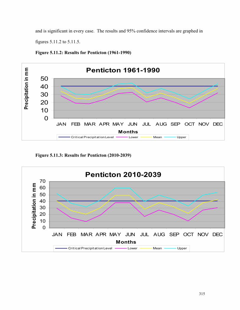
315

and is significant in every case. The results and 95% confidence intervals are graphed in

figures 5.11.2 to 5.11.5.

Figure 5.11.2: Results for Penticton (1961-1990) Figure 5.11.3: Results for Penticton (2010-2039)

Penticton 1961-1990

01020304050

JAN FEB MAR APR MAY JUN JUL AUG SEP OCT NOV DEC

Months

Prec

ipita

tion

in m

m

Crit ical Precipit at ion Level Lower Mean Upper

Penticton 2010-2039

010203040506070

JAN FEB MAR APR MAY JUN JUL AUG SEP OCT NOV DECMonths

Prec

ipita

tion

in m

m

Crit ical Precipit at ion Level Lower Mean Upper

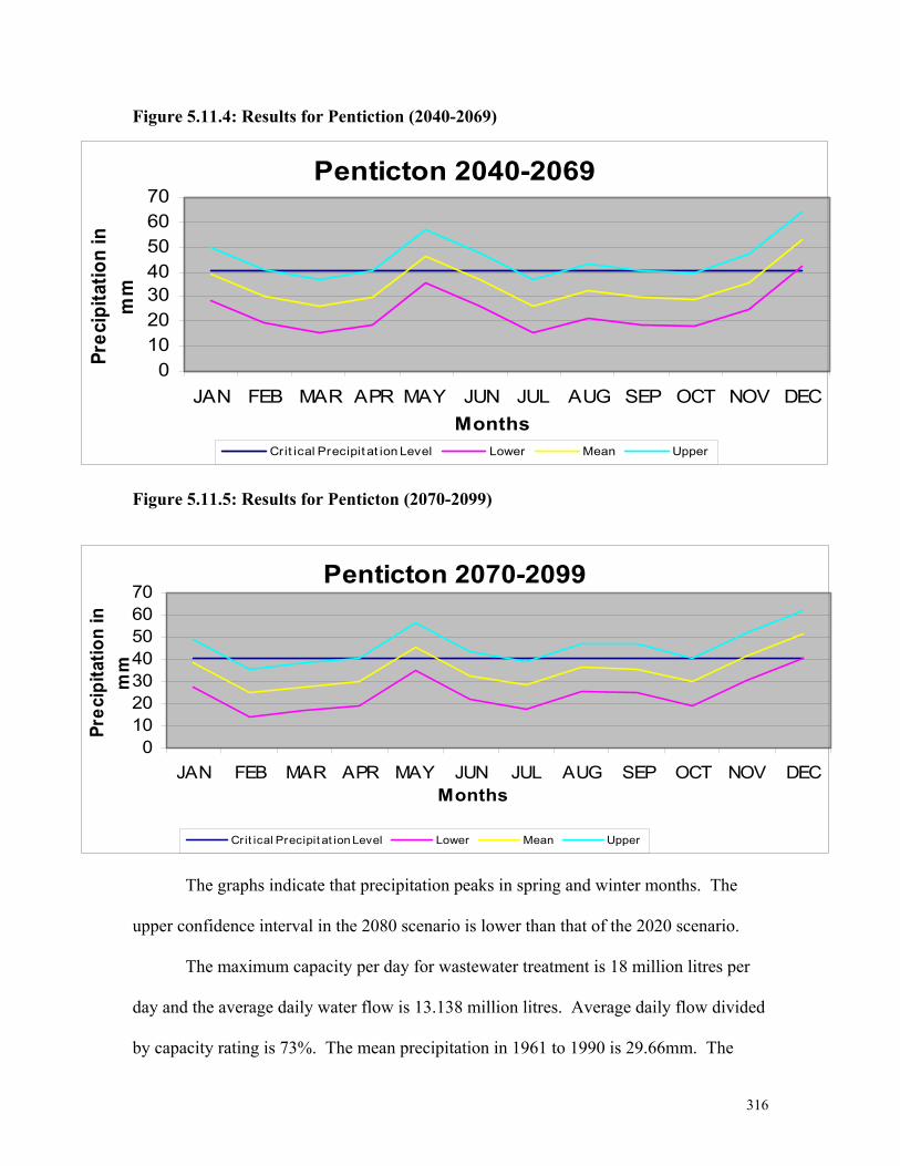
316

Figure 5.11.4: Results for Pentiction (2040-2069)

Figure 5.11.5: Results for Penticton (2070-2099)

The graphs indicate that precipitation peaks in spring and winter months. The

upper confidence interval in the 2080 scenario is lower than that of the 2020 scenario.

The maximum capacity per day for wastewater treatment is 18 million litres per

day and the average daily water flow is 13.138 million litres. Average daily flow divided

by capacity rating is 73%. The mean precipitation in 1961 to 1990 is 29.66mm. The

Penticton 2040-2069

010203040506070

JAN FEB MAR APR MAY JUN JUL AUG SEP OCT NOV DECMonths

Prec

ipita

tion

in

mm

Crit ical Precipit at ion Level Lower Mean Upper

Penticton 2070-2099

010203040506070

JAN FEB MAR APR MAY JUN JUL AUG SEP OCT NOV DECMonths

Prec

ipita

tion

in

mm

Crit ical Precipit at ion Level Lower Mean Upper

317

precipitation level in a single month that will force the treatment plants to operate at

100% is 40.6 mm. Therefore, precipitation beyond 40.6mm per month will force

wastewater into the ecosystem.

Table 5.11.4: Precipitation Exceeding Penticton’s Present Wastewater Capacity

Precipitation Exceeding Precipitation ExceedingPrecipitation Exceeding

Precipitation Exceeding

Penticton’s Wastewater Capacity

1961 to 1990

Penticton’s Wastewater Capacity

2010 to 2039

Penticton’s Wastewater Capacity

2040 to 2069

Penticton’s Wastewater Capacity

2070 to 2099 January 0 0 0 0 February 0 0 0 0 March 0 0 0 0 April 0 0 0 0 May 0 8.51 5.87 0 June 0 8.54 0 0 July 0 0 0 0 August 0 0 0 0 September 0 0 0 0 October 0 0 0 0 November 0 0 0 0.812 December 0 1.79 12.46 10.53 Totals 0 18.84 18.33 11.34 Table 5.11.5: Upper Confidence Interval Exceeding Penticton’s Present Wastewater Capacity

Upper C.I. Exceeding Upper C.I. Exceeding Upper C.I. Exceeding

Upper C.I. Exceeding

Penticton’s Wastewater Capacity

1961 to 1990

Penticton’s Wastewater Capacity

2010 to 2039

Penticton’s Wastewater Capacity

2040 to 2069

Penticton’s Wastewater Capacity

2070 to 2099 January 0 11.29 9.29 8.89 February 0 0 0.31 0 March 0 0 0 0 April 0 1.48 0 0 May 2.42 19.85 16.7 15.6 June 3.6 19.89 7.08 3 July 0 0 0 0 August 0 9 2.72 6.6 September 0 2.53 0 6.19 October 0 0 0 0.3 November 0 8.93 6.19 11.55 December 2.99 13.14 23.29 21.27 Totals 9.01 77.11 65.58 70.4

318

5.11.4: Costs of Adaptation

As shown in Table 5.11.5, precipitation exceeds the maximum treatment capacity

of 40.6mm in the 2050 scenario by 23.29mm in December. In Table 5.11.4, the mean

exceeds the capacity by 12.46 in the same month of the same scenario. This means that

capacity needs to expand by a minimum of 30% to a maximum of 57%. Based on the

costs of new treatment facilities for Prince George of $50 million (see Section 5.10.2),

the costs of adaptation range from $15 million to $28.5 million.

5.11.5: Summary and Conclusions

Penticton will face a wastewater treatment capacity shortfall, especially

considering the upper 95% confidence interval where overflows occur in several months

of the future scenarios. Overflows also occur when looking at the mean precipitation.

The costs associated with climate change adaptation range from $15 million to $28.5

million.

5.12: Yellowknife, NT 5.12.1: Drinking Water Supply

The City of Yellowknife has a population of 18,000 and is in the discontinuous

permafrost area (see Figure 5.12.1). In the past, Yellowknife used to draw its water from

Great Slave Lake, but because of increased arsenic content, they now draw from the

Yellowknife River. The draw down from the river is 2007 million cubic metres per year.

The cost of production is $5.50/1000 gallons of drinking water. The water distribution

pipes are insulated and buried below the permafrost. The temperature of water at the

intake point is 33.3oC and it is heated to 35oC. Climate change will have the effect of

reducing the heating costs of intake water because of the increase in temperature. These

319

savings in heating costs could be more than offset by the increase in the breakage of pipes

due to permafrost degradation.

Figure 5.12.1: Yellowknife

5.12.2: Permafrost and Climate Change

Mean air temperatures could rise several degrees over much of the Arctic if

carbon dioxide concentrations double. It is possible that permafrost in the discontinuous

region will disappear due to ground thermal changes. Where ground ice contents are

high, soils have the potential for instability upon thaw, such as thaw settlement, creep or

slope failure.

5.12.3: Wastewater Treatment

Yellowknife relies on a system of natural wastewater treatment where the sludge

sits in lagoons and the treated water is discharged into Great Slave Lake. The lagoon

system is a chain of small lakes and creeks covering a 13km course into Great Slave

Lake. The current sewage lagoon has a retention capacity of 2.5 million cubic metres,

which represents approximately 10 to 12 months worth of storage. In 8 to 10 years, a

2 0 0 0 2 0 0 4 0 0 K i l o m e t e r s

N

EW

S

G r i d B o x 2 6 0 - Y e l l o w k n i f e

C i t y o f Y e l l o w k n i f e

N o r t h w e s t T e r r i t o r i e s

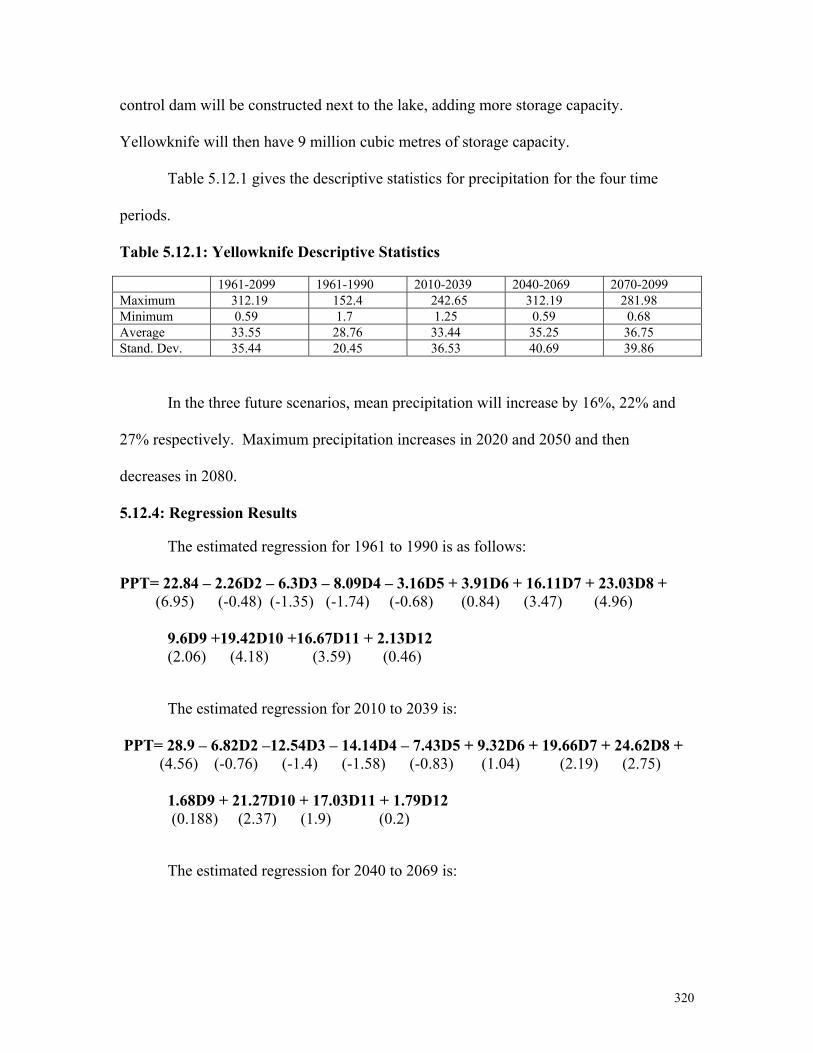
320

control dam will be constructed next to the lake, adding more storage capacity.

Yellowknife will then have 9 million cubic metres of storage capacity.

Table 5.12.1 gives the descriptive statistics for precipitation for the four time

periods.

Table 5.12.1: Yellowknife Descriptive Statistics 1961-2099 1961-1990 2010-2039 2040-2069 2070-2099 Maximum 312.19 152.4 242.65 312.19 281.98 Minimum 0.59 1.7 1.25 0.59 0.68 Average 33.55 28.76 33.44 35.25 36.75 Stand. Dev. 35.44 20.45 36.53 40.69 39.86

In the three future scenarios, mean precipitation will increase by 16%, 22% and

27% respectively. Maximum precipitation increases in 2020 and 2050 and then

decreases in 2080.

5.12.4: Regression Results

The estimated regression for 1961 to 1990 is as follows:

PPT= 22.84 – 2.26D2 – 6.3D3 – 8.09D4 – 3.16D5 + 3.91D6 + 16.11D7 + 23.03D8 + (6.95) (-0.48) (-1.35) (-1.74) (-0.68) (0.84) (3.47) (4.96)

9.6D9 +19.42D10 +16.67D11 + 2.13D12 (2.06) (4.18) (3.59) (0.46)

The estimated regression for 2010 to 2039 is:

PPT= 28.9 – 6.82D2 –12.54D3 – 14.14D4 – 7.43D5 + 9.32D6 + 19.66D7 + 24.62D8 + (4.56) (-0.76) (-1.4) (-1.58) (-0.83) (1.04) (2.19) (2.75)

1.68D9 + 21.27D10 + 17.03D11 + 1.79D12 (0.188) (2.37) (1.9) (0.2) The estimated regression for 2040 to 2069 is:

321

PPT= 23.2 – 5.41D2 –9.07D3 – 6.89D4 – 4.02D5 + 24.87D6 + 25.73D7 + 26.34D8 + (3.32) (-0.54) (-0.91) (-0.69) (-0.4) (2.52) (2.6) (2.66)

19.88D9 + 32.45D10 + 29.7D11 + 11.01D12 (2.01) (3.28) (3) (1.11)

The estimated regression for 2070 to 2099 is: PPT= 27.52 – 4.69D2 –12.7D3 – 10.1D4 – 7.51D5 + 12.05D6 + 30.96D7 + 26.37D8 + (4.06) (-0.48) (-1.32) (-1.05) (-0.78) (1.25) (3.22) (2.75)

10.04D9 + 31.52D10 + 27.44D11 + 7.33D12 (1.04) (3.28) (2.86) (0.76)

The regression results indicate that the constant increases slightly from the

baseline and is significant in all time periods. The 95% confidence intervals are graphed

in Figures 5.12.2 to 5.12.5.

Figure 5.12.2: Results for Yellowknife (1961-1990)

Yellowknife 1961-1990

0102030405060

JAN FEB MAR APR MAY JUN JUL AUG SEP OCT NOV DEC

Months

Prec

ipita

tion

in

mm

Lower Mean Upper

322

Figure 5.12.3: Results for Yellowknife (2010-2039)

Figure 5.12.4: Results for Yellowknife (2040-2069)

Yellowknife 2010-2039

0

20

40

60

80

JAN FEB MAR APR MAY JUN JUL AUG SEP OCT NOV DECMonths

Prec

ipita

tion

in

mm

Lower Mean Upper

Yellowknife 2040-2069

0

20

40

60

80

JAN FEB MAR APR MAY JUN JUL AUG SEP OCT NOV DECMonths

Prec

ipita

tion

in m

m

Lower Mean Upper

323

Figure 5.12.5: Results for Yellowknife (2070-2099)

The precipitation patterns depicted in the four time periods show that the upper

confidence interval and the mean are increasing over time. There appears to be a double

peak in July and October and a dramatic decrease in September.

5.12.5: Summary and Conclusion

Because Yellowknife draws its water directly from the Yellowknife and the pipes

are buried below the permafrost, there does not appear to be a water supply problem, nor

a cost associated with damaged pipes due to disappearing permafrost. For wastewater

treatment, Yellowknife has 10 to 12 months of wastewater storage, so an increase in

precipitation is not expected to exceed treatment capacity.

5.13: Norman Wells, NT 5.13.1: Drinking Water Supply

Norman Wells is a town of 800 located in the discontinuous permafrost zone (see

Figure 5.13.1). The water supply source is the Mackenzie River and the daily production

of water is 300 cubic metres. Two-thirds of the town is on the utilidor system, where

Yellowknife 2070-2099

0

20

40

60

80

JAN FEB MAR APR MAY JUN JUL AUG SEP OCT NOV DECMonths

Prec

ipita

tion

in m

m

Lower Mean Upper

324

water is delivered in insulated above ground pipes supported on steel piles. The water is

heated to 6-7o C. The remaining third of the town gets its water delivered by truck where

it is stored in 500 to 1000 gallon water tanks. Water is priced at $12 cubic metre

inclusive of sewage costs. Norman Wells does not have a large reservoir, and as a result,

production of water is equal to demand. Demand for water never exceeds the 500L/M

maximum capacity of water production and it is constant. The town has two km of

watermain pipeline and raw water pumps in the river and distribution pumps in the water

treatment plant. Because the town’s water source is the Mackenzie River, a drastic

reduction in rainfall would not have a huge impact on the river levels. However, if there

were repeated droughts, and the water supply became unreliable, a reservoir would most

likely be constructed.

Figure 5.13.1: Norman Wells

3 0 0 0 3 0 0 6 0 0 K i l o m e t e r s

N

EW

S

G r i d B o x 2 2 2 - N o r m a n W e l l s

P ro v i n c e o f S a s k a t c h e w a n

T o w n o f N o r m a n W e ll s

N o r th w e s t T e r r it o r ie s

N o r m a n W e l l s

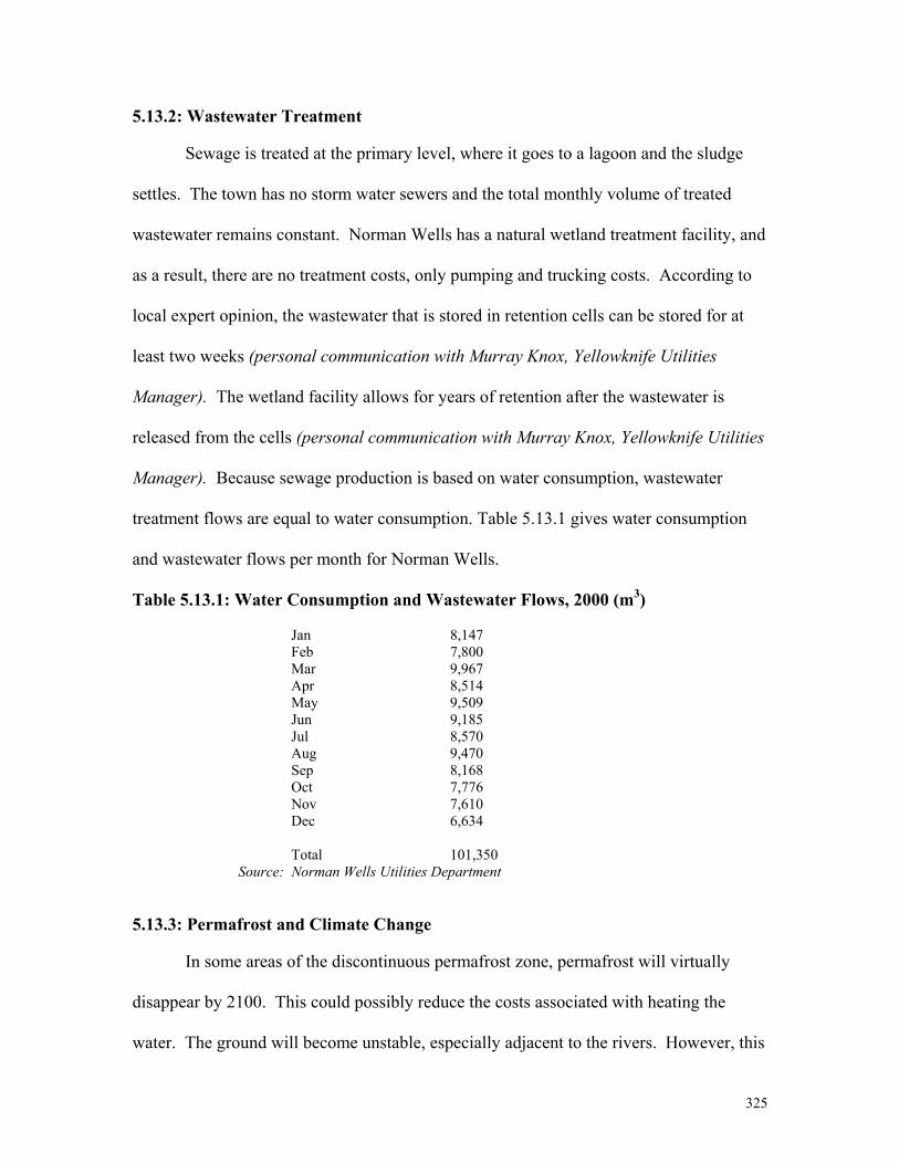
325

5.13.2: Wastewater Treatment

Sewage is treated at the primary level, where it goes to a lagoon and the sludge

settles. The town has no storm water sewers and the total monthly volume of treated

wastewater remains constant. Norman Wells has a natural wetland treatment facility, and

as a result, there are no treatment costs, only pumping and trucking costs. According to

local expert opinion, the wastewater that is stored in retention cells can be stored for at

least two weeks (personal communication with Murray Knox, Yellowknife Utilities

Manager). The wetland facility allows for years of retention after the wastewater is

released from the cells (personal communication with Murray Knox, Yellowknife Utilities

Manager). Because sewage production is based on water consumption, wastewater

treatment flows are equal to water consumption. Table 5.13.1 gives water consumption

and wastewater flows per month for Norman Wells.

Table 5.13.1: Water Consumption and Wastewater Flows, 2000 (m3)

Jan 8,147 Feb 7,800 Mar 9,967 Apr 8,514 May 9,509 Jun 9,185 Jul 8,570 Aug 9,470 Sep 8,168 Oct 7,776 Nov 7,610 Dec 6,634

Total 101,350

Source: Norman Wells Utilities Department

5.13.3: Permafrost and Climate Change

In some areas of the discontinuous permafrost zone, permafrost will virtually

disappear by 2100. This could possibly reduce the costs associated with heating the

water. The ground will become unstable, especially adjacent to the rivers. However, this

326

decrease in cost may be offset by the effects of a lower river level, in which case, intake

pipes would have to be extended to a deeper part of the river.

Table 5.13.2 gives the descriptive statistics for precipitation.

Table 5.13.2: Norman Wells Descriptive Statistics 1961-2099 1961-1990 2010-2039 2040-2069 2070-2099 Maximum 714.09 121 714.09 524.01 463.86 Minimum 0.49 2.3 1.31 0.49 1.71 Average 42.74 32.95 44.26 46.02 47.72 Stand. Dev. 49.91 22.79 57.93 57.56 51.6

The descriptive statistics for precipitation show that mean precipitation increases

slightly in the future scenarios. However, maximum precipitation increases a dramatic

490% from the baseline to the 2020 scenario. The standard deviation increases by 159%

from the baseline to the 2020 scenario.

5.13.4: Regression Results

The estimated regression for 1961 to 1990 is as follows:

PPT= 27.39 – 5.35D2 – 9.76D3 – 7.18D4 - 2.65D5 + 20.32D6 + 27.9D7 + 25.65D8 + (7.76) (-1.07) (-1.95) (-1.44) (-0.53) (4.07) (5.59) (5.14)

8.46D9 +12.25D10 – 1.99D11 –0.97D12 (1.69) (2.45) (-0.4) (-0.19) The estimated regression for 2010 to 2039 is:

PPT= 29.39 + 2.09D2 – 2.05D3 + 3.59D4 + 0.49D5 + 30D6 + 52.47D7 + 32.04D8 + (2.85) (0.14) (-0.14) (0.27) (0.03) (2.06) (3.6) (2.2)

13.63D9 + 29.53D10 + 0.5D11 + 16.09D12 (0.93) (2.03) (0.03) (1.1) The estimated regression for 2040 to 2069 is:

327

PPT= 31.8 – 4.63D2 – 6.98D3 + 5.24D4 + 12.4D5 + 27.45D6 + 51.35D7 + 46.31D8 + (3.14) (-0.32) (-0.48) (0.36) (0.86) (1.91) (3.58) (3.23)

14.49D9 + 15.61D10 – 4.58D11 + 13.96D12 (1.01) (1.09) (-0.32) (0.97) The estimated regression for 2070 to 2099 is:

PPT= 29.74 – 7.42D2 – 7.55D3 + 13.02D4 + 19.87D5 + 39.48D6 + 34.34D7 + 57.47D8 (3.36) (-0.59) (-0.6) (1.04) (1.58) (3.15) (2.74) (4.59)

+ 20.64D9 + 36.46D10 + 1.52D11 + 7.89D12 (1.65) (2.91) (0.12) (0.63)

These regressions show the likely precipitation pattern in the future scenarios and,

as such, reveal that the constant stays practically the same. The regression results and

95% confidence intervals are graphed in Figures 5.13.2 to 5.13.5.

Figure 5.13.2: Results for Norman Wells (1961-1990)

Norman Wells 1961-1990

010203040506070

JAN FEB MAR APR MAY JUN JUL AUG SEP OCT NOV DEC

Months

Pre

cip

itat

ion

in m

m

Lower Mean Upper

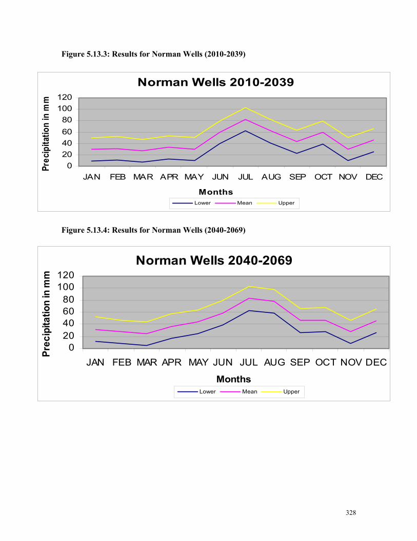
328

Figure 5.13.3: Results for Norman Wells (2010-2039) Figure 5.13.4: Results for Norman Wells (2040-2069)

Norman Wells 2010-2039

020406080

100120

JAN FEB MAR APR MAY JUN JUL AUG SEP OCT NOV DEC

Months

Prec

ipita

tion

in m

m

Lower Mean Upper

Norman Wells 2040-2069

020406080

100120

JAN FEB MAR APR MAY JUN JUL AUG SEP OCT NOV DEC

Months

Prec

ipita

tion

in m

m

Lower Mean Upper

329

Figure 5.13.5: Results for Norman Wells (2070-2099)

Because Norman Wells is in the discontinuous permafrost zone, the main factor

affecting possible climate change adaptation costs is the disappearance of the permafrost

due to higher temperatures. The above graphs give an indication of the impact on

precipitation. They show that the upper confidence level increases from a maximum of

about 60mm in the baseline scenario to over 100mm in the future scenarios. Precipitation

peaks in July and August in all scenarios.

5.13.5: Summary and Conclusions

Norman Wells will not be facing a water supply shortage as their water is

supplied by the Mackenzie River, which is a large enough source for a small population.

Wastewater treatment capacity also appears to be adequate as years of wastewater

retention are provided by the natural wetlands.

5.14: Directions for Future Research

We have carried out a number of case studies in the various ecoclimatic zones of

Canada. However, as a task for further research on drinking water supply, the coverage

Norman Wells 2070-2099

020406080

100120

JAN FEB MAR APR MAY JUN JUL AUG SEP OCT NOV DECMonths

Prec

ipita

tion

in m

m

Lower Mean Upper

330

needs to be expanded to include more case studies in Quebec, northern Ontario, New

Brunswick, Manitoba and Newfoundland. In this report we studied Montreal because of

its large urban population and investment in infrastructure, but we need to include more

rural locations in Quebec such as Sagard and St. Adolphe. Places like Val d’Or and

Chicoutimi can be included based on geographic location.

Our Ontario case studies included Toronto and Niagara but should be extended to

other communities in the northern and the eastern counties. The coverage should include

a sample of First Nations Reserves in Ontario, Saskatchewan, B.C., and Quebec.

Furthermore, as indicated in Chapter 2, there is a need to carry out further

experiments in downscaling using other methods mentioned in Chapter 2. With an

ensemble of experiments, it might be possible to see if the various methods lead to

convergent results or not. From the experiments reported here, we have excluded the

implications of evaporation and evapotranspiration. That could also be investigated.

For the prairies, we need to explore the downscaled data on snow pack and ratio of rain to

snow. Winter snow accumulation is a key surface water supply source for Canada, and

much of the U.S. As part of the forecast of global climate warming, snow pack

accumulations may vary substantially due to changes in long-term wintertime synoptic

scale precipitation combined with regional warming that may increase the rain to snow

ratio. Snowmelt contributes more effectively to stream flow than does rainfall. Hence

conversion of winter snowfall to liquid precipitation will probably result in declining

runoff. We are aware of research completed for an alpine watershed in southwestern

Alberta that combined a wide area assessment of forecast changes in wintertime synoptic

precipitation with the meso-scale alpine hydrometeorology to evaluate the impact(s) of

331

forecast climate change on mountain snow packs. The results show that modest

increases in winter precipitation will not compensate for regional changes in the rain to

snow ratios. The net result is a decline in winter accumulations of precipitation as snow;

and we expect, a decline in surface water supply. In summer, higher volumes of water

vapour in the atmosphere with a magnified greenhouse effect and warmer summer

temperatures will probably result in greater occurrence and severity of thunderstorms.

These storms could tax the capacity of existing storm water pipe networks; and will result

in greater stress on water quality and treatment facilities, particularly in regions with

combined sewer systems.

The cumulative effects of climate change on water resources may include an

increase in urban floods, increasing groundwater recharge during winter, and a decline in

average spring runoff. This means that there will be less riparian flow to dilute

contaminants. Thus there is a need to study the effects of a change in rain to snow ratio

for all prairie case studies that rely on rivers originating in the mountains. Changes in

rain to snow ratios will impose additional adaptation costs. For this reason, we believe

that it would be unwise to assume that the CGCM1 projections of precipitation (which we

relied on for this report) exhaust the research. On the contrary, all our Prairie and

Western Canada case studies show a heavy dependence on snowpack as sources of water

for rivers and basins. Therefore our results reported here should be seen only as a first

experiment and that as soon as better and more reliable data on snowpack becomes

available, the case studies reported here should be re-examined. We know that

vulnerability of water supply is likely to be most acute in the Prairie Provinces. Perhaps

this can best be done by pooling resources and establishing research links with agencies

332

such as the International Joint Commission and the National Water Resources Institute of

Canada. The research on wastewater treatment can be expanded by gathering

information on land prices for retention tanks and lagoons for major urban areas like

Toronto. We also need to estimate the costs of adaptation in other parts of the country

using location specific costs. In order to improve the estimates of the costs of adaptation,

the costs of more efficient treatment technologies such as biological nutrient removal and

UV disinfection techniques need to be included. Thus, much needs to be done to

understand the costs of adaptation to climate change for water utilities, and this report

should be seen as an important and, we hope, useful beginning.

5.15: Summary

1. The timing and regional patterns of precipitation will change, and more intense

precipitation days are likely. General circulation models used to predict climate

change suggest that a 1.5 to 4.5 degree C rise in global mean temperature would

increase global mean precipitation about 3 to 15 percent. Some of this is due to

the conversion of snow into precipitation.

2. Although the regional distribution is uncertain, precipitation is expected to

increase in higher latitudes, particularly in winter. Potential evapotranspiration

rises with air temperature. Consequently, even in areas with increased

precipitation, higher rates may lead to reduced runoff, implying a possible

reduction in renewable water supplies.

3. More annual runoff caused by increased precipitation is likely in the high

latitudes. In contrast, some lower latitude basins may experience large reductions

in runoff and increased water shortages as a result of a combination of increased

evaporation and decreased precipitation. Flood frequencies are likely to increase

333

in many areas, although the amount of increase for any given climate scenario is

uncertain and impacts will vary among basins. Floods may become less frequent

in some areas.

4. The frequency and severity of droughts could increase in some areas as a result of

a decrease in total rainfall and more frequent dry spells. The hydrology of arid

land is particularly sensitive to climate variations. Relatively small changes in

temperature and precipitation in these areas could result in large percentage

changes in runoff, increasing the likelihood and severity of droughts and floods.

5. It seems reasonable to expect seasonal disruptions in the water supplies of

mountainous areas if more precipitation falls as rain than snow and if the length of

the snow storage season is reduced.

6. The Great Lakes impact assessments suggest global warming will result in a

lowering of water supplies and lake levels and in a reduction of outflows from the

Basin. Some projections show a lowering of lake levels by up to a meter or more

by 2050. A one meter drop in the levels of Lakes Michigan and Huron in thirty

years would have a severe impact on Lake St. Clair and Lake Erie, whose levels

would drop by about 2 feet. A lake level drop of one meter in Lake Michigan

could cause thousands of municipal water intakes and wells to be moved or

extended.

7. We reported on several case studies of water utilities in the different ecoclimatic

zones of Canada, focusing on the question of the impact of climate change on the

availability of drinking water supply and capacity for treating wastewater. For

Toronto, precipitation is expected to increase, and so it is unlikely that Toronto

334

will experience a water supply problem. The City draws its water supply from

Lake Ontario, and even supposing that lake levels drop by a metre in the future

time periods, intake pipes are deep enough, and far enough into the lake.

Precipitation projections for Toronto are expected increase. Maximum

precipitation is expected to increase from the baseline period to the 2020 period

by a factor of 4. The standard deviation increases a factor of 1.7 from the baseline

period to the 2020 period. We conclude that the City of Toronto will face

adaptation costs for wastewater treatment from a low of $633 million to a high of

$9.4 billion.

8. In the region of Niagara, our analysis shows a wet autumn, followed by a wetter

winter. Wastewater treatment capacity will have to increase. We estimate the

costs will be in the range of $8 million to $24 million.

9. We found that Montréal was an exception to the general eastern seaboard case

studies. Montreal has a great deal of excess treatment capacity already built into

the system. Based on our analysis, Montréal will not have climate change

adaptation costs associated with drinking water supply and wastewater treatment.

Its drinking water source is the St. Lawrence River, which of course relies on the

Great Lakes for water supply.

10. In the case of Halifax, our projections show that maximum precipitation increases

a dramatic 315% from the baseline period to the 2020 period. It remains 149% to

232% higher in the subsequent periods. The standard deviation also increases in

the future time periods from the baseline. At present, Halifax discharges 16

mega gallons of untreated sewage per day into the Halifax Harbour. However,

335

new planned treatment capacity will come on stream in 2003. Based on this

information and our regression analysis, it appears that Halifax will experience a

wastewater treatment capacity shortfall in the future scenarios. The costs

associated with climate change adaptation will include those that expand

treatment capacity, and a rough estimate of this cost is $6.5 million.

11. We also did a sample of Prairie cities and towns. We considered Regina, Swift

Current, Humboldt, and Lethbridge. For all these prairie studies there is a need to

study the effects of a change in rain to snow ratio for all prairie settlements that

rely on rivers originating in the mountains. Changes in rain to snow ratios will

impose additional adaptation costs. We know that vulnerability of water supply is

likely to most acute in the Prairie Provinces.

12. Our West coast case studies included Prince George, and Penticton. Our analysis

indicates that existing wastewater treatment capacity in Prince George seems

adequate for the near future. Therefore, based on this analysis, there will be no

adaptation costs associated with wastewater treatment due to climate change.

13. However in the case of Penticton, we find that the city will face a wastewater

treatment capacity shortfall. The costs associated with climate change adaptation

range from $15 million to $28.5 million.

14. In Northern Canada, we included Yellowknife and Norman Wells. Because

Yellowknife draws its water directly from the Yellowknife river and the pipes are

buried below the permafrost, there does not appear to be a water supply problem,

nor a cost associated with damaged pipes due to disappearing permafrost. For

wastewater treatment, Yellowknife has 10 to 12 months of wastewater storage, so

336

an increase in precipitation is not expected to exceed treatment capacity.

15. The case of Norman Wells is more complicated. Because Norman Wells is in the

discontinuous permafrost zone, the main factor affecting possible climate change

adaptation costs is the disappearance of the permafrost due to higher

temperatures. However, Norman Wells will not be facing a water supply shortage

as its water is supplied by the Mackenzie River, which is a large enough source

for a small population. Wastewater treatment capacity also appears to be

adequate as years of wastewater retention are provided by the natural wetlands.

337

References: Wheaton, E.E., Arthur, L.M., Chorney, B., Shewchuk, S., Thorpe, J., Whiting, J., Wittrock, V. (1992), The Prairie Drought of 1988. Climatological Bulletin 26(3), Saskatchewan Research Council. Sousounis, Peter J., Bisanz, Jeanne M., (eds.) (2000), Preparing for a Changing Climate, The Potential Consequences of Climate Variability and Change. Great Lakes Regional Assessment Group. Maybank, J., Bonsal, B., Jones, K., Lawford, R O’Brien, E.G., Ripley, E.A., Wheaton, E. (1995). Drought as a Natural Disaster. Atmospheric Ocean 33 (2) 1995, 195-222. Buffalo Pound Water Administration Board (1999), Annual Report-1999, City of Regina. City of Penticton (2000), City of Penticton Advanced Wastewater Treatment Plant 2000 Operating and Laboratory Summary, City of Penticton. City of Penticton (2000), City of Penticton Water Treatment Plant Summary year 2000, City of Penticton. The Regional Municipality of Niagara Public Works Department (1999), 1999 Statistical Report. The Regional Municipality of Niagara. The Regional Municipality of Niagara Water and Wastewater Division (2001), 2001 Capital and Current Budget Presentation Items. Joint Public Works & Utilities Committee and Corporate and Financial Services Committee. The Regional Municipality of Niagara Public Works Department (2000), Water and Sewage Billing Quantities by Municipality-Report for 3rd Quarter 2000. The Regional Municipality of Niagara. The Regional Municipality of Niagara (2001), 2001 Water and Wastewater Uniform Wholesale Rates. The Regional Municipality of Niagara. Toronto Works & Emergency Services (2000), Water…Toronto treats it with Care 1999/2000 Review. Water & Wastewater Services Division. Website, City of Lethbridge, http://www.city.lethbridge.ab.ca. Website, City of Regina, http://www.cityregina.com. Website, City of Yellowknife, http://www.yellowknife.nt.ca

338

Website, Montréal, http://www.cum.qc.ca. Website, Sask Water, http://www.saskwater.com. Personal communications with the cities of Halifax, Regina, Humboldt, Lethbridge, Yellowknife, Norman Wells, Prince George, Penticton and the Regional Municipality of Niagara.

View publication statsView publication stats