the coupon-collector problem revisited
TRANSCRIPT
Purdue University Purdue University
Purdue e-Pubs Purdue e-Pubs
Department of Computer Science Technical Reports Department of Computer Science
1989
The Coupon-Collector Problem Revisited The Coupon-Collector Problem Revisited
Arnon Boneh
Micha Hofri
Report Number: 90-952
Boneh, Arnon and Hofri, Micha, "The Coupon-Collector Problem Revisited" (1989). Department of Computer Science Technical Reports. Paper 807. https://docs.lib.purdue.edu/cstech/807
This document has been made available through Purdue e-Pubs, a service of the Purdue University Libraries. Please contact [email protected] for additional information.

The Coupon-Collector Problem Revisited
Arnon Boneh and Micha HofriComputer Sciences Department
Purdue UniversityWest Lafayette, IN 47907
CSD-TR-952February, 1990
THE COUPON-COLLECTOR PROBLEM REVISITED
Amon Boneh - IOE Department, University of Michigan, Ann Arbor MI 48109-2177
Micha Hofrit - Department of Computer Science, The Technion-ITT, Haifa
May 1989
(Revised January 1990)
ABSTRACT
A standard combinatorial problem calls to cstlmate the expected number ofpurchases of coupons needed LO complete Ute collection of all possible m differenttypes. Generalizing this problem. by letting lhe coupons be obtained with anarbitrary probability distribution. and considering other related processes, theproblem has been found to model many practical siwations. The usefulness of lhismodel has been seriously hampered by !.he computational difficulties in obtainingany numerical results concerning moments or distributions. We show, followingFlajolet et al. [15], !hat Ute calculus of generating functions over regular languagesmay be applied La the problem, answer numerous questions about the samplingprocess and demonstrate their numerical efficiency. We also present a proof of along-standing folk-theorem. concerning lhe extremalily of uniform referenceprobabilities. The paper concludes with a discussion of estimation problems related
lo the engineering applications of lhis problem.
1. INTRODUcrION
The Coupon~Collector Problem (CCP) is defined as follows: A set contains m distinct objects:balls in an urn, letters in an alphabet, comics figures taken from the vaults of DisneyProductions and sold with chocolate bars... The collector samples from the set withreplacement. On each trial he has a fixed probability Pi of drawing the i-th object,independently of all past events. Several variables--or processes-are associated with thesequence of trials. all depending on the sample probability vector p = (PbPZ, ... •Pm):
Xn{p) - The item number (or 'name') drawn on the n-th trial.
tCum:ntly at thc Dcpwtrnmt of Compllcr Science, Purduc University, W. Waycnc, In. 47907.
Boneh, Hofri: Coupon Collecting Revisited... 2
T (p) - The number of the trial that completes the collection.T(k)(p) _ The number of the trial that completes the kth full collection.
T/p) - The number of the trial that completes a sub-collection of size j. Clearly T (p) =
Tm(p).Tc(p) - The number of the trial that completes a sub-collection C of specified objects.y11(p) - The number of different items observed in the first n trials.Nk(P, n) - The number of different items observed exactly k times during the first n draws.
Note: The verb 'complete' has always, in the present context. the meaning of 'complete forthe first time'. The traditional symbols E and V will be used throughout to denote theexpectation and variance of random variables.
The CCP has an extensive past; so extensive, in fact. that even a concise run-down of existingresults is well beyond the scope of this report. However, the vast majority of the results wehave seen concern the classical problem, where all the coupons have the same probability,m-1, of being drawn. This case is not our main concern. We shall have several occasionsbelow to cite works that are relevant to ours.
The CCP belongs to the family of Umproblems [25]. It is a natural framework in which to
cast combinatorial questions (and cited as such in [14]). Consequently it has seen numerousapplications, though these rarely preserve the ideal simplicity of the original CCP. Here arethree examples:
Applications of the CCP
(1) Detection of all necessary (also called 'hard' or non-redundant) constraints in a constrainedoptimization problem.
A class of algorithms for detecting such constraints, when the feasibility region is convex andof full dimension d. is based on a CCP-like sampling process. One such algorithm isPREDUCE (for Probabilistic REDUCE) suggested by Boneh and Golan [4] and incorporated inan optimization package. Each iteration of PREDUCE consists of generating a ray in randomdirection, passing tluough a randomly selected interior feasible point and which hits theboundary of the feasible region. The hit point thus created is a boundary point of the feasibleregion. and it can be shown that the facet(s) on which it is located belongs with probability oneto the hard-constraints set The algorithm proceeds to generate rays until some stopping rule issatisfied. All the consrraints not hit by that time are assumed to be redundant - possiblyerroneously. Each such a trial corresponds to drawing one coupon. The number of items isknown; however each probability Pi is not known, and is not constant, because the selectedinterior point is not necessarily the same in all trials: it can be said to be proportional to theexpected d -1 dimensional angle subtended by the corresponding facet, over the set of rayorigins. For more details on this set of algorithms see [29]. A direct determination of the nonredundant set is equivalent to computing the probabilities p, and is usually very hard, in terms
of common representations of constraint sets.

Boneh, Hojri: Coupon Collecting Revisited... 3
(2) Determining the convex closure of a set of points in R R:
This problem appears to be related to the first one, but behaves rather differently. A CCP-likedetennination of the subset of points that span the closure proceeds by generating randomn-l-dimensional hyperplanes and computing the distances of all points from each. Theextreme values (one. if they are all of one sign, or two otherwise) belong to points that are inthe desired susbset Note that if some of the closure hyperplanes contain more than n-lpoints, some of these points will never be discovered (it is simple to visualize this for n= 2with triads (or larger sets) of colinear points: the intermediate ones have a zero probability ofbeing extremally distant from any random line).
(3) The fault-detection (FD) problem in combinatorial circuits.
A combinatorial circuit may be viewed as a black box with two sets of pins: one for input andone for output. Each pin carries one bit (0 or 1) at any specified time. Loading the input pinswith a bit configuration (the input vector) produces an output vector on the output set ostensibly according to the design specifications of the circuit. However, circuits failsometimes. The standard fault model, "stuck at" [13], assumes the following:
(a) The only possible faults are of lines in the circuit that are stuck (at 0 or 1) independentlyof the input vector.
(b) Faults are rare events, and the probability of having more than one fault at anyonetime-assuming no previous faults-is negligible.
(c) FauIts occur as independent events.
Funhennore, we assume that a list of all possible fauIts is available to the test designer.
A possible way to detect a fault is to find that an input vector produced an output which differsfrom the specified output vector by at least one bit. Correct output may be produced (forcertain input vectors) by a faulty circuit. The FD problem consists of finding a list of inputvectors-as short as possible, since in critical applications the test is perfonned veryfrequently-which detect all the entries in the fault-list
One approach to the FD problem is to select random input vectors, simulate a faulty circuit anddetermine the faults detected by that input. Let n be the size of the input-pins set If all n-Ionginput vectors are generated equi~probably then Pi. the probability of detecting the i-th fault is2-n x #(of input vectors producing wrong output when fauIt i is present). Again, searching forsuch a set of vectors can be viewed as CCP-reIated: input vectors 'draw' faults at random.There is, however, the added complication that most vectors detect more than one fault,possibly hundreds. This may be represented within the CCP fonnalism either by saying thatLPi > 1, or by viewing each vector as corresponding to a batch of drawings of a random size.The distribution of the batch can be estimated by the designer. Further details may be found in
[2].
In view of these applications (and others) it is hardly surprising that the literature dealing withthe CCP and its ramifications is rich enough. It might be surprising that we found reason toadd to it, but we expect the following sections will support the need. Section 2 will survey the

Boneh. Holri: Coupon Collecting Revisited... 4
main results we find in the open literature and comment how numerical difficulties have
stymied much of the applications of the CCP.
Section 3 brings a relatively unfamiliar device-shuffling of regular languages-and shows itseffectiveness in producing numerical values for moments of various variables associated withthe CCP. It also leads us to a proof of a property of the CCP that has attained the status of afolk-theorem, but has apparently never been proved: among all possible p, the uniform vector
produces the shortest expected collection completion times..'
Section 4 brings some numerical examples and discusses the computational techniques weused. We then consider various statistical problems when CCP-like processes are employed inpractice. As the above sample applications show, the individual probabilities are usuallyunknown. Even the number of items with nonwzero probabilities is not always known to theuser. Much work has been done on several aspects of these difficulties. We summarize some of
this work and relate it to our methods.
2. RELATED WORK
(I)
-+ ...
Texts on probability commonly use the CCP as an example for elementary derivations ofexpectations. So does Feller (in [14]), who also considers the waiting times between successiveincreases of the "observed set". David and Barton consider in [11] the CCP within theirdiscussion of occupancy problems, and compute the time required to fill a given number ofboxes, remarking that the <moments are not tractable' (though it was not computationalcomplexity that seems to have concerned them, but rather the lack of explicit form for theresults). Most of the treatments we know of concern the expected time to complete thecollection, E [T(p)], and its (mainly asymptotic) properties, in the classical case, ofstochastically indistinguishable elements. The others will be mentioned during our discussions.
The best known expression for E[T(p)] is probably
m I I IE[T(p)] = L- - L + L
i=lPi l:Si<j:fmPi + Pi l:f.i<j<k:f.mPi + Pi +Pk
which is easy to prove from the inclusion-exclusion principle (see [8]) and the relationE[T(p)J = L,~Prob(T(p) > t). The earliest source we noticed for equation (I) is [11], wbo
derive it and provide some distributional results.
For the special case of a unifonn sampling vector p :::: elm, where e:::: (I, 1, ... ,1),commonly called the equalJy likely (EL) case, it is possible to obtain more compactexpressions, and for higher moments as well, since T ( elm) is representable as a sum ofindependent geomettically disttibuted random variables, the parameters of which only dependon their position in the sum - rather than on the particular items that had been sampled.
Specifically,

Boneh, Hoiri: Coupon Collecting Revisited... 5
m-l ( ')E[T(elm)]=mHm. V[T(elm)]=m2H~21,-mHm_1. E[zT(e'm)]=zII m-Jz, (2)
j=l m-lZ
The notation Hm stands for the m-th Harmonic number, :Ei~ lIi, and HJ~1 for :Ei~1111i2,
which converges rapidly to C(2) = ,,2 /6.
A. Boneh [5] has obtained a different expression for E[T(p)] by considering the differentorders in which the coupons may be obtained., and conditioning on that sequence. He finds
E [T(p)] = :E P (i)g (i), (3)i E S(N",)
where Nm is the set of the first m natural numbers and S (Nm) is the symmetric group of
pennutations of Nm • Denoting a particular pennutation by i == (i I, ... im ) he writes
m-l 1g(i)= :E ,
r=O I - LPil
k=1
(4)
for the probability of obtaining the collection in the order i and the expected time to completeit in that order, respectively. A convenience of this result is that it often produces ready rough
bounds on E [T(p)], by computing the function gO for two extreme cases: first the most likelyorder (items are sampled in order of decreasing probability). and secondly, the reverse one when the 'rarest' item is sampled first, and one ends by finding the item with highest Pi-this
can be shown to be the least likely order. The mean must be between these two, but the gap
may be substantial and we are hard put to produce from it a tighter bound.
Indeed, as David and Barton comment ruefully, the expressions in equations (1) and (3) are notamenable for numerical evaluation even for moderate m, requiring a large number ofoperations: on the order of 2m and m! respectively. Another expression of intennediate
complexity is also produced in [8]: let E {il. i 2.'" ,il } denote the expected time to observe the
entire sub-collection {i 1. i 2, . •. ,ik], then
E[T(p)]=EN ,m
and one proceeds recursively, from E {0} == 0:
I k __..:.P.::i, ,E {ib i
2• "'. il } = --+--=--+--+ L + + E (£1.i2•... ,ill - {i,}.
Pi l . . . Pij: r=IPil Pil
(5)
(6)
Brayton obtains in [7] a result equivalent to our equation (40) (the expected time to complete k
collections), and the corresponding variance. Since his main concern is in obtaining asymptotic
properties, rather than direct computation, he uses a slightly different setup: the {Pi} areassumed to be expressible as (F(i1n) - F«i-I)ln)); the dlstribution FO is then assumed toadmit a density concentrated on [0, I], that vanishes nowhere, has a finite variation andachieves its minimal value at a finite number of isolated points. The asymptotic properties turn
out to hinge on this' 'minimum set".
Boneh, Hofri: Coupon Collecting Revisited... 6
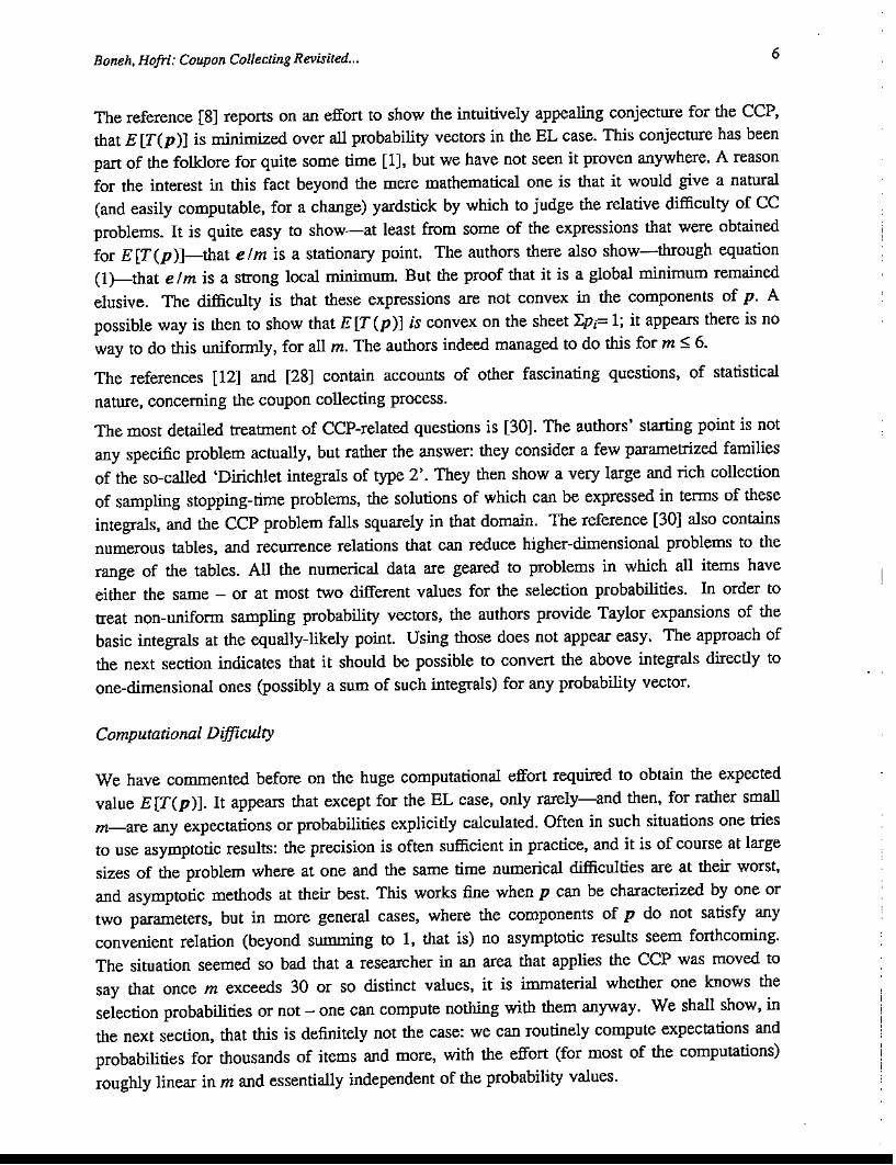
The reference [8] repons on an effort to show the intuitively appealing conjecture for the CCP,that E [T(p)] is minimized over all probability vectors in the EL case. This conjecture has beenpart of the folklore for quite some time [1], but we have not seen it proven anywhere. A reasonfor the interest in this fact beyond the mere mathematical one is that it would give a natural(and easily computable, for a change) yardstick by which to judge the relative difficulty of CCproblems. It is quite easy to show-at least from some of the expressions that were obtainedfor E[T(p)]-that elm is a stationary point. The authors there also show-through equation(l}--that e 1m is a strong local minimum. But the proof that it is a global minimum remainedelusive. The difficulty is that these expressions are not convex in the components of p. Apossible way is then to show that E [T (p)] is convex on the sheet 4Jj= 1; it appears there is noway to do this uniformly, for all m. The authors indeed managed to do this for m:5: 6.
The references [12] and [28] contain accounts of other fascinating questions. of statisticalnature, concerning the coupon collecting process.
The most detailed treatment of CCP-related questions is [30]. The authors' starting point is notany specific problem actually, but rather the answer: they consider a few parametrized familiesof the so-called 'Dirichlet integrals of type 2'. They then show a very large and rich collectionof sampling stopping-time problems, the solutions of which can be expressed in terms of theseintegrals, and the CCP problem falls squarely in that domain. The reference [30] also containsnumerous tables, and recurrence relations that can reduce higher-dimensional problems to therange of the tables. All the numerical data are geared to problems in which all items haveeither the same - or at most two different values for the selection probabilities. In order totreat non-unifonn sampling probability vectors, the authors provide Taylor expansions of thebasic integrals at the equally-likely point. Using those does not appear easy. The approach ofthe next section indicates that it should be possible to convert the above integrals directly toone-dimensional ones (possibly a sum of such integrals) for any probability vector.
Computational Difficulty
We have commented before on the huge computational effort required to obtain the expectedvalue E [T(p )]. It app= that except for the EL case, only rarely-and then, for rather smallm-are any expectations or probabilities explicitly calculated. Often in such situations one triesto use asymptotic results: the precision is often sufficient in practice, and it is of course at largesizes of the problem where at one and the same time numerical difficulties are at their worst,and asymptotic methods at their best. This works fine when p can be characterized by one ortwo parameters, but in more general cases, where the components of p do not satisfy anyconvenient relation (beyond summing to 1, that is) no asymptotic results seem forthcoming.The situation seemed so bad that a researcher in an area that applies the CCP was moved tosay that once m exceeds 30 or so distinct values, it is immaterial whether one knows theselection probabilities or not - one can compute nothing with them anyway. We shall show, inthe next section, that this is definitely not the case: we can routinely compute expectations andprobabilities for thousands of items and more, with the effort (for most of the computations)roughly linear in m and essentially independent of the probability values.

Boneh, Hofri: Coupon Collecting Revisited...
3. A NEW APPROACH
7
Recently, Flajolet et al. presented in [15] a new approach, or rather, a novel point of view ofthe CCP, which resulted in a computationally superior expression for the expected duration ofthe CC activity, which they obtained as well. We show both below. Their approach may beviewed in a wider context, as a way to compute probabilities for various variables defined interms of sequences of independent sampling from a finite population. The same approach wasbriefly mentioned earlier by Comtet in [10]. In this framework there is a natural way to
answer more detailed questions about the sampling process.
Mter showing the outlines of the method, its application will be illustrated by posing andsolving a sequence of such questions. In this section we only provide analytic expressions. Thepower and utility of the method lie largely-as the authors in [15] observe-in the amenabilityof these to numerical evaluation. Computational techniques for this purpose is the topic of
Section 4.
We collect here the questions, so that their inter-relationships will be easier to perceive:
(1) In a sample of length n, what is the probability that item #i occurs at least ri times? In the
CCP the rj are specialized to be all 1.
(2) The same question as (1), but now we ask only about a subset of the items, C cA.
(3) What is the probability of finding in a sample of size n at least r items repeated each at
least k times?
(4) What is the expected number of different items drawn in a sample of size n?
(5) What is the expected time until j ~m different coupons have been sampled?
(6) What is the expected time until j~m different coupons have been sampled at least k times
each?
(7) What is the expected time until j ~m specified different coupons have been sampled?
(8) How many coupons will be sampled exactly r times, or more than r times, before T(p)?
(9) Is the expected time a good estimate of the required time? - we want more informationabout the distribution of T (p), so we can answer the questions: with what probability willT(p l exceed E [T (p l] by a certain fraction, or in still another way: how long do we have
to sample to obtain all coupons with a probability exceeding a?
(10) What is the distribution of Nl(p,n), defined as the number of coupons observed exactlyonce in the first n trials? In the next section we explain the significance of this variable.
This is what we need in order to solve the above:
Strings Over A Finite Alphabet
Let A = {al' ... , am} be an alphabet. The set of all finite words of letters from A is denotedby A·. A subset of A· is called a language, and a word in a language will be genericallydenoted by w. The letter aj is associated with the probability Pj' and a word w is assumed to
Boneh. Hofri: Coupon Collecring Revisired... 8
carry two types of weights: one is the standard additive weight, chosen here to be the size ofthe word in letters, and denoted by Iw I. The second is a "probabilistic weight" that equalsthe product of the probabilities of its letters: 1t(W):;::: TIajEwPj' Define for a language L the
following probability generating functions (pgf):
$L<z)= L It(w)z'w',weL
(7)
(8)
The functions $L(Z) and ~L<z) are called the ordinary and exponential pgf's of L, respectively.They are related through the so-called Laplace-Borel transform:
$L(z) ~ f ~L(zt)e-Idt_t>D
These are not the usual pgf's used in probability theory for the distributions of (discrete)random variables, but observe that [zn] $L<z) is the probability that a random word of size n,from A" is in the language L. This formalism does not support directly the notion of a
random word of arbitrary size.
We define two operations on languages: concatenation and shuffling, which are usedextensively below; they expose two properties of the pgf's we defined and exhibit the need for
both types of functions.
1. The concatenation of two functions, L 1 and L2' is a language L, written as £=L 1L2' suchthat each word of L is formed by concatenating a word from L2 to a word from L 1, to formw=w l.w2. The operation is "well-defined" iff it has the property of unique factorization: for
each w E L there exists a unique pair WI, w2, such that Wi E Lj, and W=Wl·WZ·
Proposition 1: IT the operation £=L 1L2 is well-defined, then
(9)
2. The operation of shuffling two languages is defined recursively as follows: Two languagesare shuffled by shuffling all their words pair-wise. Two words are shuffled by merging theirletters in all possible manners, while retaining the original order in each. This recursive
definition can be formally expressed as follows:
WoE=EoW=W, (e is the null word.)
a.wl 0 b.W2 = a. (WI 0 b.wz)Ub. (a'WI 0 wz)
L 1o£2= U WloW2.WI eLl
w2 EL 2
a, b E A, Wi E Lj,(10)
The operation is "well-defined" for languages that use disjoint subsets of A - that is, employ
different alphabets. When this is the case, it is straightforward to show that
Proposition 2: If the operation L = LID L 2 is well-defined, then
(11)
All our applications of this tool have the following format: the statement of the problem is

Boneh. Hofri: Coupon Collecting Revisited... 9
reinterpreted-sometimes this is straightforward and occasionally involves intermediatesteps-as a specification of a language H from A·. The words of H are shown to beconstructible from simple components by concatenation and shuffling. The building-blocks will
be such that their pgf's are easy to compute directly, and Propositions 1 and 2 will provide thepgf's of H, from which we shall <read off' the desired answers. We show here one such
construction that is used extensively below:
Define a k-hit as the occurrence of a letter k times (or more) in a word. We shall see later thatit is useful to be able to compute the probability that a random word of a specified size has k~
hits for exactly q distinct letters.
The basic construct is the following one: Let Hq, It: be a language with only such words inwhich exactly q letters recur at least k times, and the other m-q letters appear at most k-ltimes. Then introduce the following notation for um-Ietter languages:
ad = {E, a, a 2 , ••. ,ak - 1 } , a~ =ak·a· • (12)
where a2 is shorthand for the word aa. etc., and a· is the supremum of all ad. The crux ofthe approach is that this notation provides the following expression for all the words of Hq, k:
(13)
(15)
(16)
where the union is over all two-set partitions of A, indexed by I and J: I = (i 1, , iq ),
] =lh..... im-q}, In] =0. IU] =Nm. This may seem merely a complicated way torepeat the verbal specification of Hq, k> but since the exponential pgf's of the constituentelements are straightforward to write, we shall obtain immediately that of Hq,k: Let ek(z)
denote the incomplete exponential function
k ziek(z) = k -., ' (14)
i=O t.
then. since a· contains exactly one word of each size j:::: 0, the desired exponential pgf's are:
j ja~ PI Z zp·U i (z) =k-',- =e '- ek-l(zPi),
j'" I·
The sets I and J involve disjoint alphabets; hence, summing over products of these exponential
pgf's, we obtain for the exponential pgf of Hq, k:
~q,k(Z) = k II (e'Po - ek-l (ZPi) II (ek-l (zPj).I,JiEI jEJ
This ungainly sum allows for a more compact representation; we need for it the notation
Ixrlf ex), for the coefficient of xr in the power series development off ex):
~q.k(Z) = [uqrrr [ek_l(ZPi) + u(e'P, -ek-l(zp;J)]. (17);=1
If we are interested in probabilities of words of a specified size n, this is all that is needed. Ifthe interest is in the sum of these probabilities over words of any size-or in CCP formulation:of any sequence of trials-it is more convenient to use the ordinary pgf, and with the Laplace-

Boneh, Hofri: Coupon Collecting Revisited...
Borel Transform we find
10
$q, k(Z) = [u q] f1>0
mIT [ek-l (zip,) + u(e"P; - ek-l (ZIp,»)]e-'dt.j=l
(18)
When all the probabilities are equal, at 11m. the expressions are naturally much neater. The
summation in equation (16) is over (~) identical tenns, yielding
~q.k(Z) = (~)(e,'m - ek-l (zlm»)q (ek-l (zlm)t-q • (19)
and similarly for the ordinary pgf.
The utility of the the machinery outlined above will be now demonstrated in providing answers
to problems (I) through (10).
(I) The probability ofdrawing coupon #i at least r, times in n trials, i= I,m
The samples satisfying this requirement make up a "language" in which each word contains
the letter aj at least 'j times. Denote this language by H(p, r). Then in analogy with equation
(13)
( >r >r >r)H(p.r)= al loaz 2. 0 ... oam'" . (20)
where the ar,· are defined in equation (12). The exponential egf of the collection of uni-Ietter
d >r,. p,' (P)·th () 0 hwar s aj IS e -e,_l jZ, Wl e-l' == ; ence,m
~(p, r; z) = IT(eP,'- e,,1 (PiZ»),i=l
and the desired probability is given bym
pep, r; n) = n 
Boneh, Hoiti: Coupon Collecting Revisited... 11
kpep r C· n) = n '[z']e,(I- Pclrr(eP(,,' - e I~ . z))• • ,. r(i)-llJ"(l) .
i=l(24)
Naturally this may be obtained from equation (22) when r (i) = 0 is inserted there, for 1~ i ~ k.
(3) The probability of scoring k-hits for r coupons in a sample of size n
A k-hit is defined above as the occurrence of a letter at least k times in a word. We also writethere the exponential pgf of the language Hr,k, which contains words with exactly r k-hits these are equations (16) and (17). The construction is indeed similar to the one above, butsince the items are not specified, we need to sum over all possible rwout-of-m sets.
What is the probability of scoring at least r k-hits? The temptation to use the language
H(p,r,k)= u [(ai;"oai;"o ... oal;') o (A-I)'], (25)/: l/I=r
should be resisted, since many words are repeated in this specification. The way to follow is to
use equation (17). Define Yn(p, k) as the number of k-hits in a word of size n. Then
.mProb[Y,(p, k) = j] = n ![z'u1Jrr(ek_l (PiZ) + u(eP
,'- ek-l (Pi Z)))i=l
[z'ui ] f IT(ek-l (Pizt) + U (e P'" - ek-l (pizt)))e-'dt,l~ i=1
(26)
where we have used in the last line the Laplace-Borel transfOITIl. The required answer is thenLr:S:j:s:mProb[Yn(p, k) = n. There does not seem to be any essentially simpler way ofexpressing this truly complex combinatorial quantity. Even in the EL case, while it lookssimpler, the computational effort is essentially the same.
(4) The expected number of different coupons drawn in a sample of size n
(27)= n ![z'j aa b(u, z) I '
U u=1
This problem calls for the evaluation of E[Yn(p, 1)]. The answer is available from elementaryconsiderations (see e.g. [9]), but it should be instructive to use the present apparatus torecapnrre it. Since equation (26) gives the probabilities, we have
E[Y,(p, I)] = Ljn
Boneh, Hofri: Coupon Collecting Revisited...
a m ePiZ_1au b(l, z) = b(l, z\~ eP"
Finally
m=e'L(l-e-P,').
i=l
12
(29)
m 1 (1 - Pi)'" mE[Yn(p, 1)] =nlL(-, - ,) = L[1- (l-pi)n],
i=l n. n. i=l
as we should expect. In Section 4 we consider some properties of this value.
(5) The expected time to draw a sub-collection of size j [15]
Consider the following set of equalities:
E[T/p)] = LProb(T/p) > n) = LProb(Yn(p, 1) < j).n2:0 n~
(30)
(31)
(34)
The second equality results from the fact that the two compound events (Tj(p) > n} and(Yn(p, 1) < j} consist of precisely the same sequences of trials, and hence have the same
probability. Now we prepare to use equation (26):j-l j-l
L Prob(Yn(p,l) <j)= L LProb(Yn(p,l)=r)=L [L Prob(Yn(p,l)=r)). (32)n~ n~ r=O r:=O n2:0
Anned now with the necessary ingredients, equations (26) and (18) give, specialized to k= 1
E[T/P)]=ji! LProb[Yn(p, l)=r] =ji! [u'] lfi(l+u(eP"-l))e-'dr. (33)r=O n2:0 r=O t~ j=}
Since the integrand is an m-degree polynomial in u, the case j=m simplifies greatly: in this
case we need the sum of the coefficients of ur for all r except r=m, which is n~l (ePit
- 1).The sum of all the coefficients is simply the value of the right-hand side at U= 1, and we find:
E[Tm(p)] = E[T(p)] = 1 [e' - fi(e P,' - l)]e-'dr,t2:0 i=l
and since exp(-t)= exp(-:Epjt), we further simplify to
E[T(p)] = 1[1- fi(l - e-N)]dt.t~O j=}
(35)
We have thus obtained a computationally convenient fonn for the expected duration of T (p).
Equation (35) has a particularly simple fonn in the particularly simple EL case of unifonn
probability vector:
E[T(elm)] = 1[1- (1- e-IImt]dt.,>0
(36)
Interestingly enough, an integral nearly identical with the one in equation (36) (with thetransfonnation of the integration variable to x=e-t ) may be found in an unpublished report bytbe authors of [8]. Observe, moreover, that the equality of the integral in (35) to the right-hand

Boneh, Hofri: Coupon Collecting Revisited... 13
side of equation (1) is straightforward.
The computational advantage of this integral over the sums we encountered in Section 2 isenormous: instead of dealing with 2m oscillating terms, we integrate a bounded, smooth,everywhere-positive function. It is true that the range of integration may be tremendous as well
(we shall discuss this below), but the function is smooth enough for an integration routine withlocally adaptive step-size to compute it with several hundreds of function evaluations, under
very stringent accuracy requirements.
There is interest also in finding the time to 'almost complete' the sampling, that is, for valuesof j that are very close to m, and the same approach that led to equation (35) applies, with a
somewhat heavier price. Thus, for example, we find
(37)
Note that with some care the computations of these quantities can be still kept to be essentially
linear in m.
Remark: We found it instructive to consider the two quantities, computed in problems (4) and(5), side by side. Both may be viewed as functions in the (sampling. duration, number ofcaptures) plane, but with the relation of independent/dependent variables reversed. Consider
these coordinates as providing the abscissa and ordinate, respectively, as shown in the generic
Fig.!.
The engineering (and statistical) significance of the two functions are also very different: The"detection curve", given by equation (30), shows the expected number of detected items as afunction of the sampling duration; we find it more suggestive to think of the fraction of the
DetectedFraction
1 . --- ---. -- ------------ ------ - --- ------ --------
E [T(P)] Sample size
Fig. 1: Detection-temporal relationships

Boneh, Hofri: Coupon Collecting Revisited... 14
items that have been captur~ rather than their number. Then the "sample duration curve",computed via equation (33), gives the expected duration required to complete a specifiedfraction. Equations (35) and (37) above give expressions for two points on this curve;computing each is linear in m, but obtaining the entire curve still appears infeasible when thenumber of distinct probabilities is large. Note that the :first curve extends to infinity (along theabscissa), while the second one tenninates in the point (E [T (P )], 1). Another way todistinguish the two curves is to consider how they compare with individual experiments. Thuspoints of the :first curve represent average of samples scattered along the ordinate, while thesecond one features averages of horizontal scatter. We conjecture the duration curve to liealways (that is, for any p) entirely above the detection curve.
(6) The expected time to draw a size j sub-collection k times [7]
For j=m. k=2, in the EL case, this problem has been known as the "double Dixie cupproblem" (after the product that carried the collected coupons). Holst provides an answer forthe EL case in [23], and comments on earlier derivations of that result, extending to 1960, allconsidering complete collections (i.e. j =m), and-except [7]-the EL case. Other referencesof interest (all essentially concerned with limiting properties of E[T(elm)] and variationsthereof) are [16], [26] and [27].
The required expected value is obtained exactly as for Problem (5):
E [Tj·) (p)] = L Prob(TjkJcp) > n) = L Prob(Yn(p, k) < j).1l~ n~
Tbe same approach lbat produced equations (33) and (35) will now provide
j-I j-I / mE[Tjk)(p)] = L L Prob[Yn(p, k) =r] = L [u'] nO + u (eP,'- e._l (p,t)))e-'dt,
r=O n~O r=O r~ i:::1
and
E[T(·)(p)] = /[1- ficl- e-P"ek-l(P,t))]dt.l~ ;=1
(38)
(39)
(40)
Computing this expected time is of roughly lbe same difficulty as lbat of E[T(p)], andincreases sub-linearly with k. Equation (40) is precisely the result already obtained in [7].Brayton also considers asymptotic results (as m-7oo); his results there depend on a particularmodel he chose to generate p, so we shall not go into them in any detail, except to mentionlbat in lbe EL case he obtains E[T(·)(elm)] = m[logm + (k-l)loglogm + C.].
(7) Expected time to draw a specified sub-collection of size j
While the formulation appears rather different than problem (5), and may be seen as asignificant generalization, it can be handled almost identically. Let the required subset be
C E A. As above,
Boneh. Hofri: Coupon Collecting Revis;red... 15
j-lE[TcCp)] = LProb[TcCp) > n] = LProb[W.(C,p) < j] = L (LProb[W.(C,p) =k]J,(41)
n~ n~ k=O n~
where Wn(C,p) is the number of coupons from C observed in a sequence of n drawings. Stillas before, except that different words contribute and therefore we construct a differentlanguage: Rk(C) is a language containing only words in which exactly k items of C appear.
Using equations (12) and (13) it can be written as
Hk(C) = U (a~l 0 a~' 0 •.. 0 a~' ) 0 (A - C)", (42)IcC
where the union is over all I = {ail' ... , ail} C C, so that Rk(C) has the exponential pgf
II> () "<' IT ('P, I) '(I-Pel~~C Z =... e - e , (43)
];III=kiel
where Pc = LieC Pi . Let us write C={a(l).... ,aU)}· The same manipulations that led us to
equation (35) provide
hcCZ) = [uk] fi[1 + u(e'P''> _1)]e,(I-Pel,;=1
and for the expectation we find
E[Tc(p)] = ji$~c(l) = ji / [Uk] nJI + u(e'P, _1)]e,(I-Pele-'dt,k=O k=O t~ ;=1
= /[1- IT(I-e-P''>')]dt,l~ ie C
in complete analogy with equation (35).
(8) The distribution of r-hits during T (p)
(44)
(45)
Denote by Mr(p) the number of coupons observed at least r times once T(p) is over. Wordsthat contribute to Prob(M,(P) = k) temtinate with a letter appearing for the first time andcompleting the collection. Specifying this letter as al, the corresponding prefixes form the
language Lr. k(l) that has the structure
L (I) U ( ".". ".) (+<' +<' +<' )r k = ail aai,. 0 ... o ail 0 ajl oah 0 .•. Oaj -H' (46). IcA-{l} '"
where I = (a· ... a·) a· eA -I - {I} for 1~c5m-k-l and a+<r is a languageI]' • Il' Jc '
consisting of words of sizes between 1 and r-1. Lr,k(l) has then the exponential pgf
1\,. k(l; z) = L IT (e'P' - e,_1 (ZPi)) IT (e,-I (zPj) - I).I iel jeA-I-{I}
m (47)= [ukJIT [e,_I(zPi) -I + u(e'P; -e,_I(zPi))]'
i=1i~l
and the ordinary pgf
Boneh, Hofri: Coupon Collecting Revisited... 16
(48)
The complete words that contribute to Prob(Mr(p) = k) are formed by concatenating the aboveprefixes with al. The letter has the ordinary pgf P1Z. and hence, by Proposition 1 and theobservation that the probabilistic weight of each word is actually equal to the probability of
obtaining the corresponding sample,
(49)
For example, the probability that the maximal frequency obtained by any coupon does not
exceed r-l, is given by the readily computable expression
m f mProb(M,(p) ~ 0) ~ kP, e-' II (e'_1 ('Pi) - I)dt.
1=1 t;;1) i=1"~l
Also, the expected number of such multiplicities is given by
E[M,(p)] ~ mi'Lkp,[Ukj f IT [e,-I('Pi) - I + u(e'P, - e,_I('Pi))]e-'dt.k=ll=1 f~ i=1
i~l
(50)
(51)
This integral can be simplified to some extent. Since Ek[uk]f(u) ~f'(I), we get
E [M,(p)] ~ f LP,e-tp, L [I - e-'P1e'_1 ('Pjl] II (I - e-tp')dt. (52)r~ i=1 j=1 i#, I
j#
Changing the order of summation and integrating by pans:
m (pt)r-l mE[M,(p)]~m- f kP,e-tp, ('_ )1 II (I-e-tp')dt. (53)
1;;:01=1 r 1. i=1i~l
The language defined in equation (46) can be used to evaluate directly the expectation of T(P),
rather than the circuitous way that led us to equation (35). It results however in a
computationally less-efficient expression for the expectation.
(9) On the distribution of T (p).
Actually we have obtained already expressions for the distribution of T(P): from the discussionleading to E[T(p)] - see equation (31), we find for the tail probabilities of T(p), specializing
eq"ation (26) to k~ I, thatm-l m
Prob[T(p»n]~Prob[Y"(p,I)<ml ~ kn
Boneh. Hofri: Coupon Collecting Revisited... 17
(m pz m
Prob[T(p) >n] = n ![z"l e' - II(e ; - I») = I - n '[z"lII(eP;' - I). (55)i=l i=l
which is as simple as we could ask for. The last equality is also a specialization of equation
(22).
Consider now another property of the distribution - the variance V[T(p)]. We use the relationE [T2(p)] =E">o(2n+ I)Prob[T(p» n] =212 + E[T(p)]. To compute /2 we have the choiceof using the exponential pgf or the ordinary one. The first produces
m/2 = LnProb[T(p) >n] = Ln(l- n![z"lII(eP"-I»).
n2:1 n~l j=l
The second one yields
(56)
f m [ m ( pi/2= LnProb[T(p»n]= LPjt I-II I-e-;)]dt.
n?:l 12:0 j=l i=li;t.j (57)
mIT(t) '" II(I - e-P;I).
j=l
Then V[T(p)] =212 +E[T(p)](I-E[T(p)]). Both expressions for /2 are cumbersome tocompute; the first one is of the same type as equation (35): it could be decomposed tosomething like equation (1), involving 0 (2m) terms, most of which would be vanishinglysmall and hard to estimate. The second would be - numerically - less troublesome. It is verysimilar to the integral required for E[T(p)], but in order to keep the computation time linear inm, we have to separate the evaluation of the product, as shown there.
(10) On the distribution of N I (n).
Here we are interested in the number of letters that occur exactly once in a word of size n. Thewords that contribute to Prob(N1(n)=r) are similar to those we constructed in problem (3):
and hence
H(p,r)= U [(ai,oai,o ... o a') o (A-I)'I].I: III=r
~,(Z) = L IIZPiII(e'P, - ZPj),I iEI jT
m 'PProb[N 1(p, n) = r] = n ![z"u']II(e ; + (u - I)zp;).j=l
(58)
(59)
(60)
In this case as well, numerical evaluations are not simple, and unless the components of p havean analytically tractable form one is unlikely to obtain even useful asymptotic estimates. Theexpectation is sttaightfonvard to obtain either from equation (60) or from elementary
considerations, and equals

Boneh, Hofri: Coupon CoUecting Revisited...
mE[N1(p, n)] = nLpi(I - p,)n-l
i=1
18
(61)
Sobel et al. in [30] bring up a few more questions that are of interest in this context, all ofwhich can be answered with the tools used above - one just has to create the appropriate
'languages'. Here is an example that gives the flavor:
Given two sets, C and D, what is the probability of hitting r of the first before capturing k
of the second?
Improvements of the algorithm PREDUCE described in Section 1 lead to CCPs with themultiple completion-sets criterion: Let (Ad, 1~i~r be r subsets of A. What can be said aboutthe number of trials required for the elements of at least one of them to be all obtained? Onecan easily write expressions as above, but direct evaluation is typically not easy.
We now twn to the minimization conjecture mentioned above:
Proof of the Conjecture
The conjecture that E[T(p)] is minimal when the probability vector p is uniform is ofpractical interest because it would then provide an easily computable lower bound when theactual probabilities are unknown (as is the case in many applications). We mentioned thedifficulties encountered in showing it from equation (1), but starting with equation (35) it is assimple as one can ask for. Denote the integrand in that equation by f (t, p). We observe thatf (t, p) is everywhere positive, and shaH show that it is minimized-uniformly in t-for theEL probability vector elm. The desired result follows. The minimization problem
=rrlinf (t,p) = min[I - n(I - e-P,')]p~ p<:.O i=1
is clearly equivalent to the problemm
max[I- f(t,p)] = max n(I- e-N )p~ p~ i=1
=Subject to LPi = 1,
i=1
=Subject to LPi = 1.
i=1
(62)
(63)
The last relation shows that at the optimum p > O. Then f (t,p) is strictly positive, and since thelogarithm function is strictly monotone increasing over the positive reals, we can replace the
above with the equivalent problem
= tmax 10g[I - f (t,p)] = max Llog(I - e -P, )p>o p>o i=l
=Subject to LPi = 1.
i=l(64)
The last problem is clearly equivalent to searching for the usual saddle-point of the Lagrangian
m t m mUp, A., v) " Llog(I - e-P' ) + A.(LPi - 1) + L viPi·
i=l i=l i=l
(65)
Now it is immediate to see that for any t > 0 the Lagrangian L (P, A., v) has a stationary point atthe uniform p (with the values for A. and v there uniquely defined). Moreover: in the p-space itis every-where concave (its Hessian is diagonal, with negative elements only), hence that point
Boneh. HoJri: Coupon Collecting Rellisited...
is a global maximum for equation (63), and a global minimum for E [T (p )].
4. COMPUTATIONAL ASPECTS AND NUMERICAL EXAMPLES
19
A major consideration in the treatment presented above-indeed, the reason it was done in thefirst place-is its suitability for numerical work. We describe some computations, and remarkon the significance of the numerical results.
For engineering problems that can be modelled by the CCP one needs estimates in particularfor the following quantities:
(a) The expectation of T(p).
(b) Dispersion measures of T (p), where tail probabilities are possibly the most useful.
(c) The tradeoffs between length of sampling and the probabilities of detecting givenfractions of the items.
(d) A rather different issue arises in applications: the vector p is frequently unknown. Weshall consider some results that are relevant in this case.
(a) The expectation ofT(p)
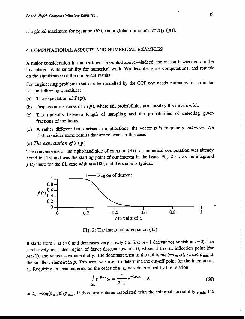
The convenience of the right-hand side of equation (35) for numerical computation was alreadynoted in [15] and was the starting point of our interest in the issue. Fig. 2 shows the integrandf (t) there for the EL case with m= 100, and the shape is typical.
I -, .....:...1- Region of descent -I
0.8
f (t) ~:~0.2O+------.----,-::::::::=--r----,------.-
o 0.2 0.4 0.6( in units of Iu
0.8 I
(66)
Fig. 2: The integrand of equation (35)
It starts from 1 at t=O and decreases very slowly (its first m-1 derivatives vanish at t=O), hasa relatively restricted region of faster descent towards 0, where it has an inflection point (form> 1), and vanishes exponentially. The dominant tenn in the tail is exp(-pmint), wherepmin isthe smallest element in p. This term was used to determine the cut-off point for the integration,tu' Requiring an absolute error on the order of E, tu was determined by the relation
f -pod I -'0"e """- I = --e "1""""- = E,Pmin
or (u=-log(PminE)IPmin. If there are r items associated with the minimal probability Pmin the

Boneh, Holri: Coupon Collecling Revis;(ed... 20
cut-off point needs to be pushed to tu := -log(PminE/r)IPmin. In our work we routinely alsointegrated also along the interval (tu,1.5t/.l)' to estimate the actual error. We used for E thevalue 10-7, which is far too stringent than is necessary in actual applications, but was selectedin order to drive the integration procedures hard. The integration was done with the routinequancB from [17], which uses 8-point Newton-Cotes integration with locally-adaptive step size.Sample results are shown in tables 1 and 2.
m 10 100 1000 10,000 100,000
E[T(p)] 56.24 1856.52 41,288.83 739,709.57 11,670,512.01
mHmlogm 63.6 2388 51,707 901,472 13,919,295
'. 571 17,406 281,140 4,053,471 54,629,467# Evalu. 177 161 177 193 145
Table 1: E [T (p)] for the Zipf distribution.
The probability vector used in table 1 is the Zipf distribution, with Pi := 11iHm . The second linecorresponds to the estimate mHmlogm, suggested in [15] as an asymptotic estimate ofE [T (p )]. This estimate clearly tracks the correct values, but produces a substantialoverestimate that seems to be little influenced by the increase of m, at least up to 105. Thecomputational effort is roughly linear in m (and is essentially independent of the particularprobability vector, when all the probabilities are distinct). The last line reports the number offunction evaluations used in the integration, and it is practically constant in m, with theoscillations depending on the location of the region of descent of the integrand (which is fairlysmall compared with tu ) with respect to the evaluation points selected by the integrationroutine.
Table 2 presents results for a different distribution that arises in applications: the so-calledLinear distribution. There Pi = 2i1m(m+l). For comparison, the second line brings thecorresponding expected values in the EL case.
m 10 100 1000 10,000 100,000
E[T(p)] 68.985 6338.74 628,226.33 62,766,148.84 6,276,050,044.96E[T(elm)] 29.929 518.74 7485.47 97,876.06 120,901.46
'. 1107 124,458 14,635,349 1.692x10⁹ 1.923xlO"# Evalu. 177 225 225 209 209
Table 2: E[T(p)] for the Linear distribution.
In a sense this distribution is an inversion of the picture presented by the Zipf distribution:there as here we have many probabilities of very close values, but for the Zipf distribution it isthe small probabilities that are close, whereas for the linear one it is the higher values that arenearly uniform. The change this causes in E[T(p)] is dramatic: it is now quadratic in m, andcan be shown to have the asymptotic value m (m+ 1)(2,qV3 - 3) " 0.6275987m (m+ 1). Thisresult was stated first-without proof-in [11]. The proof consists in showing that for this

Boneh, Hofri: Coupon Collecting Revisited... 21
(67)
particular probability distribution, the integral in equation (35) can be written in the limit
m~ 00 as ~lLk~lbkXkdx, where bk is a well-known number-theoretic function, specifying thedifference between the number of partitions of k with even number of distinct parts, and thenumber of such odd-sized partitions. In [19, p.14] it is shown that bk is (_1)71 when k equalsn(3n+1)/2 for some integer n, and vanishes otherwise. The rest is routine integration. Theasymptotic estimate agrees with the exact value to six decimal places already for m= 100.
The influence of the last few hard-to~get items on the expected sampling time is considerable:To demonstrate the effect of those rare items, we used equation (45) to compute the expectedtime to draw-for m= IOOo-all but the IO items with smallest probabilities, and obtained
E [Tc~"l = 106,387.30, about one sixth of the corresponding E[T(p)].
(b) Dispersion measures and tail probabilities
The variance of T (p) is somewhat more expensive to calculate-using equation (57)-than theexpected value, hence we only computed it for m= 1000 for the above distributions, andevaluated its variance ratio. We found the values 0.20521 and 0.72201 for the Zipf and theLinear distributions, respectively. (For the EL case it equals -V163745017485. = 0.17134.) It israrely the case that tail probabilities are easier to compute than moments, and the situationhere, despite the innocent appearance of equation (55), is no exception. A direct approach is to
use the Cauchy integral formula, and write
I r mProb[T(p) >n] = 1 _..!!.-=:- fP z-n-1II(eN - I)dz.
2m C i=l
, 2•= 1 - E...:.... jz-nrr(eP,Z
- 1)d8,21t 0 i=l
The integration, however, except for small (and relatively uninteresting) values of m and n isnumerically unstable, because the integrand oscillates, assuming very large positive andnegative values along the path. The larger values occur however only at values of z with smallargument, hence the integral is a good candidate for estimation by the saddle-point method:writing the integrand in the first line of equation (67) as exp(hn(z)), we have
n(eP;R. - I)'=1 (68)
Prob[T(p) >n] = 1 - n! 1-' ,R~+ v2rr;hn;"(Rn )
where Rn is the root of the equation hn;'(z) = O. We experimented with this expression - andthere were no surprises: the computations are straightforward, and reasonably accurate, but form ex.ceeding a few scores, and n larger than m by a single order of magnitude, one mustarrange the computations in equation (68) very carefully, to avoid a numerical disaster. Anexample is the EL case, where it is very easy to show that !J. E n+ 1 - Rn: > 0 tends to zerorather fast (it is smaller than 1 already for n ::::: mlogm, that is - for all values at which one
would consider looking for tail probabilities). We find there

Roneh. HOfri.: Coupon Collecling Revisiled... 22
(69)n!R~-n
Prob[T(p) >n] = 1 - -l!.-::mC"1~""2,,-(-n-+":1):"(l---l!.-lm-) .
Solving for Rn is easy, but getting reasonable accuracy for tail probabilities below 0.01 called
for multiprecision arithmetic.
The distribution of the number of unsampled coupons after n drawings approachesasymptotically, for large m and n, the Poisson distribution with parameter :Lr;l exp(-nPi)· Holstet at. have shown in [24] that when all the probabilities satisfy c 11m S Pi S C2/m, the rate ofconvergence to this distribution is bound from above by C·max(m-e
1/c
2, m-I/Zlogm, for some
constant C.
(c) Sampling Tradeoffs
Consider equation (30). We can get closed-form results from it mainly in the EL case, for thefollowing derivation. When n = E [T(elm)] = mHm we find, for large m
1 mil -HE[Yn(elm,l)]=m[l-(l--) m]=m(l-e m)
m(70)
The approximation of Hm by logm + y (Euler's constant) will suffice here; the error is(12mr' + 0 (m -2), and y= 0.57722... We find that the expected number of items detected bythe time the CC would expect to finish is extremely close to m, at m-e-'Y::::: m-0.56146.., withthe shortfall essentially independent of m. The standard deviation of T(elm) is by equation(2) approximately equal to m"r!6 " 1.28255m. It is a suitable uuit of comparison withE[T(elm)]. and so we compute the expected number of items found inE [T (e 1m)] + kxnmr!6 trials. We present the expected shortfalls below. When the expectednumber of detected items is m-a, then a is the shortfall, given in Table 3:
k a
-4 94.9148-3 26.3227-2 7.30004-1 2.024510 0.561461 0.155712 0.04318
3 0.011984 0.00332
Table 3: Expected shortfalls for sampling in the EL case
To appreciate the values in this table, note first that these shortfalls are virtually independent ofm. Secondly, the length of E [T(e 1m)] measured in standard deviations is quite small: it comesto 3.6 for m= 100, 5.386 for m= 1000 (where all of the approximations used above are quite

Boneh. Hofri: Coupon Collecting Revisired... 23
tight), and 7.1813 and 8.9766 for m at 10" and 105 , respectively. For the last case, e.g., thetable provides that in the first five standard deviations (approximately 55% of the expectedtotal sampling time), the expected number of detected items is 99905.1. On the other hand, tobe fairly confident that all the items are obtained the collector must endure a very longsampling sequence.
For other reference distributions we do not have such closed expressions, but experimentationrevealed very similar patterns, usually-and surprisingly-with smaller shortfalls.
Cd) Unknown probability vector p.
In many applications that are modelled by the CCP. the vector p is not known to the collector.This raises several questions of interest.
What does the item-drawing process tell us about p? Of course, one could simply count thenumber of times each item comes up in the sampling process, and use it to estimate theprobabilities. Good estimates, especially for the smaller probabilities, require an inordinatelylong sampling time, typically much longer than E[TCp)] Csee [21]). We could settle for less,and just inquire about the general shape of the vector: is it close to elm? Or to the Zipf
distribution? Or to any other attracting distribution? The process N 1(n) that was considered inproblem (10) appears interesting in this context. It requires very little overhead in terms ofbook-keeping, compared with maintaining counters for all items, and is informative. To show
this we computed its expected value for several types of p, for a few values of m and plottedthe results, in Fig. 3.
For all the distributions, the curve for m =10 peaks higher and sooner than the others. The highdispersion of the curves for the Zipf distribution is curious, as the others do not exhibit such aphenomenon. At least between these families one might distinguish as the sampling process
continues.
Another situation of interest arises when some of the components of p might be zero! A goodexample of such situation is the redundancy problem introduced as application (1) in Section 1.
Out of the m constraints,let q be hard ones. The other r = m-q will never show up, regardless
of how long the optimizer samples. Since the value of r is not known a priori, it is reasonableto ask about a stopping rule which does not depend on the number of sampled items, and inparticular - not on its closeness to m. In [28] Robbins makes the following remarkable
suggestion, aUributed there to an observation by A.M. Turing: Let Xj(n) be a random variablecorresponding to item #i, that assumes the value zero if that item has been sampled by the n-thtrial, and I otherwise. The quantity of interest for the optimizer, that measures "what remains
to be done''. is U(p,n) = I:.PiXi(n) - a random variable that is unobservable. by definition. (Its
reciprocal is sometimes called the resistance of the process.)
However, let us compute its expected value: Prob(Xi(n) = 1) is simply (I-Pit, hence

Boneh. HolTi: Coupon Collecting Revisited... 24
solid - EL case, m =10,50,100,500
----
-,-
dashed - Zipf dist., m =10,50,100,500
dotted - Linear dist., m =10,50,100,500i~'-3_~ -I;.....tI !" ... ::S~"'IO; - _
" '-............. --f, //)': .... ....II / \.. '.. .... ....
,I I \.. '.. ............
'
1111 "I",· '.. .. ...... ...... .. .......-
I ' ,,'" .... .. ...... ..'I"~ ,... ...1,[ \_'" ..,.... ....'/ ... .. L.... ....,I '.. - ....I, 'i-... .. ....
1/1 ·;;;;;1.... .... .. ..........
~, 1'1;,...........I '. ...., -l "'~~···I"'::~7;:·.,,:o..-
' .. ::: .~~':.;::.:::;;....~::.:.::::::::::'-,
0.1
0.3
0.4
o 2 4 6n in units of m
8 10
Fig. 3: The fraction of items observed exactly once .vs sample size
mE[U(p,n)] = LPi(l- Pi)"'
j=l(71)
Comparing this with equation (61) we find
IE[U(p,n)] = --E [N 1(p,n+ I)).
n+1(72)
Now, N 1(p,n+l) is certainly observable, from which the optimizer has an unbiased estimateof U(p,n.). The curves in Fig. 3 should be viewed again in the light of this characterization.We can do even better, by considering the variance of U(p.n):
mE[U2 (p,n)] =E[(DiXi(n))(~pjXj(n))] =LPf(l- Pi)" + LPiPj(l- Pi - Pj)"' (73)
i j i=l i#
It is also easy to find observables that estimate these expressions. Let N2(p.n) be the numberof items drawn exactly twice in the first n trials, and N(2)(p,n) be the number of distinct pairs
observed once (in any order) in that sequence (it clearly simply equals (~I ). Then immediately

Boneh. Hotri: Coupon Collecting Revisited...
mE[N2(p,n)] ~ G)LPT(l- Pir2
i::ol
25
(74)
E [N (2)(p,n)] ~ (~)LPiPj(1 - Pi - pjr2
r~j
Hence an unbiased estimate of V[U(p,n)] is given by cn~2r2 (Nz(p,n+2) +N(z)(p,n+2))
- (n+I)-2Nr(p,n+I).
Of even more interest is the evaluation and estimate of the variance of of the differenceU(p,n) - N 1(p,n+ l)/(n+ 1). This is available from results above, except the expected value
of their product, which is easy to obtain (and to estimate via equation (74» as well:
mE[U(p,n)N 1(p,n+ I)] ~ LPT(l- Pi)" + L(l- Pi - Pjr1(n+ I)p/I - pjl- PiPj). (75)
i::ol i~j
Surprisingly, it is even possible to estimate the number of new items the sampler may expect tofind in the next n' trials, once it has done n of those and dutifully recorded all of Nk • Good and
Toulmin show in [18] that the suitable estimator is given by
n'B,,-.n
(76)
This is typically useful at a stage of the sampling process when the first few Nk have not yetdecreased too much towards their ultimate value - zero. This result is used in [12] to estimatethe number of words of English Shakespeare knew, on the basis of his available output...
5. CONCLUSION
We have shown that for the CCP one may barter time for precision in obtaining numericalresults. In some cases this was relatively easy, but some of the expressions we derived are veryill-conditioned; they may of course be handled by any computational method that uses userdefined precision, but then we are likely to run into substantial computation times again. Mostof the expressions share however the fortunate characteristic, that it is precisely those largevalues that obstruct direct numerical evaluation, that would make them susceptible forasymptotic analysis. The way equation (68) was obtained is one example, and we expect to
extend this approach to several more of the results that were derived above.
There is a different, intriguing point of view of the sampling process, that is suggested byequation (35). Consider m independent Poisson counting processes, with parameters {Pi}'Since the probabilities sum to one, the expected number of counts per time unit is one as well;let us then establish an equivalence between the 'time' of those processes and the 'time' of thecoupon sampling process - which is simply the number of sampled coupons. The probability
that each of the Poisson processes produces at least one count by time t is II;;1 (1 - e-Pi').Hence the expected time until they all count (at least once) is given by equation (35).Similarly, equation (37) is the expected time to get m-l distinct counts. The asymptoticdistribution for the number of unsampled coupons, shown at the end of section 4(b), is

Boneh, Hofri: Coupon Collecting Revisited... 26
obtained by this coupling as well.
Holst shows in [23] a deeper relationship between these two schemes, and obtains a resultwhich is related to Problem (1) above. We shall use his notation. Let {Zd denote the timeintervals between successive counts, and In - the type of the nth arrival. We consider thestopping time Tk;m, which is when exactly k of the processes have reached---or exceededtheir quota (the process of type i has a quota of Tj). Also, we let Ti denote the time untilprocess i fills its quota, and clearly T j has the Erlang distribution with parameters (Tj,Pi)· Nowhe observes that Tk;m is simply the kth order statistic of {TdF;l· If Tk;m falls at the Wk;m th
arrival, we have thatW~;m
Tk;m = 1; Zj, (77)j=l
where Wk;m and the Zj are all independent. Now Holst finds for the egf of both sides
wJ:;oo
E[exp(xTk;m)j = Ew[Ez[exp(x 1; Z) IWk;m]], (78)j=l
and since the interarrival periods are iid - exp(l), this gives
-w. 9)E[exp(xTk;m)] =E[(I-x) ~], (7
from which there is an immediate relationship between the moments of Tk;m, which arestraightforward to compute (in principle, that is) and the (ascending) factorial moments of
Wk;m'
There is a different way to relate the two processes, which uses the Poisson transform [20]. LetA (t) be a functional over the Poisson processes up to time t, such as a moment of somecounter or a probability related to some stopping time, and let An be the correspondingfunctional with respect to the first n samples, of the discrete process. The value of A (t) can be
computed by conditioning on the number of 'arrivals' during t, since given that there occurredn arrivals, they are distributed among the coupon types according to the same underlying
multinomial distribution. Hencen
A (i) = 1; Prob(n arrivals during i)An = 1;e-'-'-;-An .n~ n~ n.
(80)
Hence A (t)e I is the egf of {An}' if we can compute the first - the second is immediately
available:
An = n 
Bonek. Hofri: Coupon Collecting Revisited... 27
a panacea; for example, it is as complicated to evaluate the moments of any order statistic ofthe (Til, when the rates (probabilities) are distinct, as it is to evaluate the right-hand side ofequation (33). Hence it will not reduce the time required to compute the 'sample duration
curve' discussed in the Remark following equation (37).
ACKNOWLEDGMENT
We are grateful to David Aldous for drawing our attention to reference [23].
REFERENCES
[1] D. Aldous, private communication, 1989.
[2] P.H. Bardell, W.H. McAnney, 1. Savir: Built-in test for VISI - pseudorandom techniques,
J. Wiley, 1987.
[3] P.I. Bickel, I.A. Yahav: On Estimating the Number of Unseen Species - How ManyExecutions Were There? Technical Report No. 85 Dept. of Statistics, DC Berkeley California
June 1985.
[4] A. Boneh: "PREDUCE" - A Probabilistic Algorithm Identifying Redundancy by aRandom Feasible Point Generator. Chapter 10 in M. Karwan, V. Lotfi, I. TeIgen, S. Zionts
(Eds.): Redundancy in Mathematical Programming, 1983.
[5] A. Boneh: One Hit-Point Analysis (Private Communication, November 1986).
[6] A. Boneh: Prediction of the Fault-Detection Curve in Combinatorial Circuits. IBM Israel
Technical Repon 88.253 September 1988.
[7] R.K. Brayton: On the Asymptotic Behavior of the Number of Trials Necessary to Completea Set with Random Selection. Jour. Math. Anal. Appl. 7, 31~1 (1963)
[8] R.J. Caron, M. Hlynka, J.F. McDonald: On the Best-Case Perfonnance of ProbabilisticMethods for Detecting Necessary Constraints. Windsor Mathematics Report WMR-88-02,Dept. of Mathematics and Statistics. University of Windsor, Ontario, Canada, February 1988.
[9] R.I. Caron, J.F. McDonald: A New Approach to the Analysis of Random Methods forDetecting Necessary Linear Inequality Constraints. Math. Prog., 43, 97-102 (1989).
[10] L. Comtet: Advanced Combinatorics, D. Reidel, Dordrecht, 1974.
[11] EN. David, D.E. Barton: Combinatorial Chance, Charles Griffin & Co. London, 1962.
[12] B. Efron, R. Thisted: Estinoating the Number of Unseen Species: How Many Words Did
Shakespeare Know? Biometrika, 63, 435-447 ,(1976).
[13] R. D. Eldred: Test Routines Based on Symbolic Logical Statements. Jour. Assoc.
Comput. 6, #3,33-66 (1959).

Boneh, HoIri: Coupon Collecting Revisited... 28
[14] W. Feller: An Introduction to Probabiiity Theory and its Appiications, Vol. 1, 3rd Ed. J.
Wiley, 1968.[15] Ph. Flajolet, D. Gardy, L. Thimonier: Birthday Paradox, Coupon Collectors, CachingAlgorithms and Self-Organizing Search. INRIA RC #720. August 1987.
[16] L. Platte: Limit Theorems for Some Random Variables Associated with Urn Models.
Ann. ofProbab. 10,927-934 (1982).
[17] George E. Forsythe, Michael A. Malcolm, Cleve, B. Moller: Computer Methods for
Mathematical Computations. Prentice-Hall 1977.
[18] I.J. Good, a.H. Toulmin: The number of New Species. and the Increase in Population
when a Sample is Increased. Biometrika 43, 45--63 (1956).
[19] P. Henrici: Appiied and Computational Complex Analysis, Vol. 2, J. Wiley & Sons, 1977.
[20] M. Hom: Probabilistic Analysis of Algorithms: On Computing Methodologies forComputer Algorithms Performance Evaluation. _Springer-Verlag. New York 1987.
[21] M. Hom, H. Shachnai: Self-Organizing Lists and Independent References - A StatisticalSynergy. The Departtnent of Computer Science, the Technion TR#524, October 1988.
[22] L. Holst: A Unified Approach to Limit Theorems for Urn Models. J. Appl. Probab. 16,
154-162, (1979).
[23] L. Holst: On Birthday, Collectors', Occupancy and Other Classical Urn Problems. Intern.
Stat. Rev. 54, 15-27, (1986).
[24] L. Holst, J.E. Kennedy, M.P. Qnine: Rates of Convergence for Some Coverage and UrnProblems Using Coupling. J. Appl. Probab. 25,717-724, (1988).
[25] N.L. Johnson, S. Kotz: Urn Models and their Applications. An Approach to Modern
Discrete Probability Theory. John Wiley, New York, 1977.
[26] DJ. Newman, L. Shepp: The Double Dixie Cup Problem. Amer. Math. Month., 67, 58---61
(1960).[27] A. Renyi: Three New Proofs and a Generalization of a Theorem of Irving Weiss. Magy.
Tudo. Akad., 7, 203-213 (1962).
[28] RE. Robbins: Estimating the Total Probability of the Unobserved Outcome of an
Experiment. Ann. Math. Stat. 39,256--257, (1968).
[29] RL. Smith, J. TeIgen: Random Methods for Identifying Nonrednndant Constraints.Technical Report 81-4, Departtnent of IOE, University of Michigan, Ann Arbor 1981.
[30] M. Sobel, V.RR. Uppulnri, K. Frankowski: Dirichlet Integrals of Type 2 and TheirApplications, Vol. IX in the series Selected Tables in Mathematical Statistics, Amer. Math.
Soc. 1985.