the deep roots of volcanoes: models of magma dynamics with applications to subduction...
TRANSCRIPT

The Deep Roots of Volcanoes: Models of Magma
Dynamics with Applications to Subduction Zones
Richard Foa Katz
Submitted in partial fulfillment of therequirements for the degree
of Doctor of Philosophyin the Graduate School of Arts and Sciences
COLUMBIA UNIVERSITY
2005

c© 2005
Richard Foa Katz
All Rights Reserved

ABSTRACT
The Deep Roots of Volcanoes: Models of Magma Dynamics with
Applications to Subduction Zones
Richard Foa Katz
In this thesis I present research on the dynamics of the partially molten mantle
with applications to magma genesis and transport in subduction zones. Subduction
zones are the most complex tectonic setting for magma genesis on Earth. To model
and understand them requires a study of the fundamental physics and chemistry
of the mantle beneath their associated volcanoes where melting occurs and magma
migrates through the pores of the rock toward the surface. These partially molten
regions of the mantle control the overall chemical evolution of the Earth as well as
the characteristics of the volcanic systems that they feed. At tectonic boundaries,
the mechanical interaction of partially molten mantle with lithospheric plates, and
with large-scale mantle convection, influences the dynamics and organization of plate
tectonics. These interactions can be described within the framework of the magma
dynamics equations derived by McKenzie (1984).
One important question concerns how partially molten regions are organized. It is
generally accepted that magma resides in the interconnected pores between crystals
that make up mantle rock. Less well understood, however, is the spatial distribution
of porosity: is it uniform or localized? To address this issue, chapters 2 and 5 con-
sider mechanical and chemical interactions in the fluid–solid system of the partially
molten mantle that, through instabilities, produce heterogeneous, localized distribu-
tions of fluid from an initially uniform mixture. The mechanical instability results
from porosity-weakening of the solid matrix (Stevenson, 1989; Spiegelman, 2003),
however the orientation of bands of high porosity is shown here to be controlled by
the balance between porosity and strain-rate weakening. The chemical instability re-
sults from reactive dissolution of mantle matrix by upwelling fluids (Aharonov et al.,

1997; Spiegelman et al., 2001). Using a new, parameterized pseudo-phase diagram
for the generic rock–water system, I show that hydrous fluids rising off the slab in a
simple subduction zone model channelize and locally modify the temperature field.
These two chapters demonstrate that, relative to predictions by homogeneous mod-
els, localization of melt in the mantle can radically alter permeability structure, melt
transport rates, thermal structure, chemical transport and even large-scale deforma-
tion of the magma/mantle system in subduction zones and other settings of magma
genesis.
Subduction zones represent the most complex instance of partial melting in a
tectonic/volcanic system. Observations of arc volcanoes raise a suite of questions
about the dynamics active at depth below them. To address these questions requires
comprehensive, self-consistent models of magma genesis and transport in subduction
zones. Even a basic model that incorporates fluid and solid flow, reaction and tem-
perature evolution will be complex, challenging to construct, and require advanced
computational resources. In Chapter 2 I describe a computational approach for fluid
flow in a deforming mantle matrix; in chapter 3 for modeling mantle flow with highly
variable non-Newtonian viscosity; in Chapter 4 for melting systematics of the hy-
drous magma/mantle system; and in chapter 5 for temperature-dependent reactive
flow of hydrous fluids/magma. Each of these contributes to the development of a
comprehensive model of subduction by addressing computational challenges and ex-
posing complex behavior such as sharp viscosity gradients and strong localization
phenomena.
The central themes of this thesis are localization phenomena and the effects of
complex rheology on the magma–mantle system. Calculations presented here demon-
strate that both of these are likely to play an important role in shaping the processes
of magma genesis and transport in partially molten regions of the mantle and, par-
ticularly, in subduction zones. Many questions are raised by this work, especially
regarding the observable signature of predicted localizations. This work represents
fundamental progress on understanding the generation and organization of magma in
the mantle.

Contents
Table of Contents i
List of Tables vi
List of Figures vii
Acknowledgments xviii
Dedication xxi
1 Introduction 1
1.1 Modern challenges in understanding subduction . . . . . . . . . . . . 3
1.2 Theoretical framework . . . . . . . . . . . . . . . . . . . . . . . . . . 6
1.3 Computational framework . . . . . . . . . . . . . . . . . . . . . . . . 9
1.4 The content of this thesis . . . . . . . . . . . . . . . . . . . . . . . . . 12
2 The Dynamics of Melt and Shear Localization in Partially Molten
Aggregates 17
2.1 Introduction . . . . . . . . . . . . . . . . . . . . . . . . . . . . . . . . 17
2.1.1 Past work with magma dynamics theory . . . . . . . . . . . . 20
i
2.2 Coupling shear deformation and fluid flow . . . . . . . . . . . . . . . 21
2.2.1 Linear analysis . . . . . . . . . . . . . . . . . . . . . . . . . . 21
2.2.2 Numerical solutions . . . . . . . . . . . . . . . . . . . . . . . . 31
2.3 Comparison with data . . . . . . . . . . . . . . . . . . . . . . . . . . 34
2.4 Discussion . . . . . . . . . . . . . . . . . . . . . . . . . . . . . . . . . 35
2.5 Conclusion . . . . . . . . . . . . . . . . . . . . . . . . . . . . . . . . . 36
3 Mantle Flow and Thermal Structure in a Kinematic Subduction
Zone Model 37
3.1 Introduction . . . . . . . . . . . . . . . . . . . . . . . . . . . . . . . . 37
3.2 Governing equations and numerical solution . . . . . . . . . . . . . . 38
3.3 Results . . . . . . . . . . . . . . . . . . . . . . . . . . . . . . . . . . . 41
3.4 Discussion . . . . . . . . . . . . . . . . . . . . . . . . . . . . . . . . . 46
3.4.1 Magma genesis in subduction zones . . . . . . . . . . . . . . . 46
3.4.2 Magma focusing in subduction zones . . . . . . . . . . . . . . 48
3.5 Conclusions . . . . . . . . . . . . . . . . . . . . . . . . . . . . . . . . 52
4 A New Parameterization of Hydrous Mantle Melting 55
4.1 Introduction . . . . . . . . . . . . . . . . . . . . . . . . . . . . . . . . 55
4.1.1 Basic structure of the parameterization . . . . . . . . . . . . . 57
4.2 Mathematical Formulation . . . . . . . . . . . . . . . . . . . . . . . . 58
4.2.1 Anhydrous Melting . . . . . . . . . . . . . . . . . . . . . . . . 58
4.2.2 Hydrous Melting Extension . . . . . . . . . . . . . . . . . . . 60
4.3 Experimental Database . . . . . . . . . . . . . . . . . . . . . . . . . . 68
ii

4.3.1 Anhydrous . . . . . . . . . . . . . . . . . . . . . . . . . . . . . 68
4.3.2 Hydrous . . . . . . . . . . . . . . . . . . . . . . . . . . . . . . 70
4.4 Model Calibration . . . . . . . . . . . . . . . . . . . . . . . . . . . . . 71
4.4.1 Anhydrous melting . . . . . . . . . . . . . . . . . . . . . . . . 71
4.4.2 Hydrous melting . . . . . . . . . . . . . . . . . . . . . . . . . 72
4.4.3 Free Parameters and Missing Constraints . . . . . . . . . . . . 73
4.5 Comparison with other models . . . . . . . . . . . . . . . . . . . . . . 75
4.6 Testing and validation . . . . . . . . . . . . . . . . . . . . . . . . . . 76
4.6.1 Adiabatic upwelling beneath mid-ocean ridges . . . . . . . . . 76
4.6.2 Arc Melting . . . . . . . . . . . . . . . . . . . . . . . . . . . . 81
4.7 Summary . . . . . . . . . . . . . . . . . . . . . . . . . . . . . . . . . 82
5 Reactive hydrous melting and channelized melt transport in arcs 89
5.1 Introduction . . . . . . . . . . . . . . . . . . . . . . . . . . . . . . . . 89
5.2 Reactive melting . . . . . . . . . . . . . . . . . . . . . . . . . . . . . 91
5.2.1 Chemistry . . . . . . . . . . . . . . . . . . . . . . . . . . . . . 91
5.2.2 Physics . . . . . . . . . . . . . . . . . . . . . . . . . . . . . . . 96
5.3 Results . . . . . . . . . . . . . . . . . . . . . . . . . . . . . . . . . . . 99
5.3.1 Flow from the slab surface to the core of the mantle wedge . . 100
5.3.2 Flow from the slab surface to the lithosphere overlying the wedge102
5.4 Discussion . . . . . . . . . . . . . . . . . . . . . . . . . . . . . . . . . 106
5.5 Future work . . . . . . . . . . . . . . . . . . . . . . . . . . . . . . . . 110
5.6 Conclusion . . . . . . . . . . . . . . . . . . . . . . . . . . . . . . . . . 112
iii

6 Discussion 114
6.1 Summary . . . . . . . . . . . . . . . . . . . . . . . . . . . . . . . . . 114
6.2 Open questions . . . . . . . . . . . . . . . . . . . . . . . . . . . . . . 116
6.2.1 Buoyancy effects . . . . . . . . . . . . . . . . . . . . . . . . . 116
6.2.2 Rheological effects . . . . . . . . . . . . . . . . . . . . . . . . 117
6.2.3 Experimental constraints . . . . . . . . . . . . . . . . . . . . . 117
6.2.4 Magmatic focusing . . . . . . . . . . . . . . . . . . . . . . . . 118
6.3 Conclusions . . . . . . . . . . . . . . . . . . . . . . . . . . . . . . . . 119
Bibliography 121
A Ridge Migration, Asthenospheric Flow and the Origin of Magmatic
Segmentation in the Global Mid-Ocean Ridge System 136
A.1 Introduction . . . . . . . . . . . . . . . . . . . . . . . . . . . . . . . . 136
A.2 Model description and solution . . . . . . . . . . . . . . . . . . . . . 139
A.3 Melting and melt focusing . . . . . . . . . . . . . . . . . . . . . . . . 141
A.4 Results . . . . . . . . . . . . . . . . . . . . . . . . . . . . . . . . . . . 142
A.5 Discussion . . . . . . . . . . . . . . . . . . . . . . . . . . . . . . . . . 143
A.6 Conclusions . . . . . . . . . . . . . . . . . . . . . . . . . . . . . . . . 145
B A Semi-Lagrangian Crank-Nicolson Algorithm for the Numerical
Solution of Advection-Diffusion Problems 148
B.1 Introduction . . . . . . . . . . . . . . . . . . . . . . . . . . . . . . . . 148
B.2 Algorithms . . . . . . . . . . . . . . . . . . . . . . . . . . . . . . . . . 149
iv

B.2.1 Basic Algorithms . . . . . . . . . . . . . . . . . . . . . . . . . 150
B.2.2 Hybrid Schemes . . . . . . . . . . . . . . . . . . . . . . . . . . 152
B.3 An analytic test problem . . . . . . . . . . . . . . . . . . . . . . . . . 154
B.4 Results . . . . . . . . . . . . . . . . . . . . . . . . . . . . . . . . . . . 157
B.5 Discussion . . . . . . . . . . . . . . . . . . . . . . . . . . . . . . . . . 162
B.5.1 Adaptive Interpolation Method . . . . . . . . . . . . . . . . . 163
B.6 Conclusions . . . . . . . . . . . . . . . . . . . . . . . . . . . . . . . . 166
v

List of Tables
3.1 Empirically determined parameters for diffusion and dislocation creep(Karato and Wu, 1993; Hirth and Kohlstedt , 2003) used in equation(3.5). . . . . . . . . . . . . . . . . . . . . . . . . . . . . . . . . . . . . 40
4.1 Summary of experimental peridotites (anhydrous experiments only).a Modal cpx not known or not available. The mean of the other peri-dotites, 16%, is assumed for computations here. b Constructed by com-bining mineral separates from the Kilbourne Hole Xenolith. . . . . . . 69
4.2 Summary of parameters and values. . . . . . . . . . . . . . . . . . . . 744.3 Summary of variance reduction. a Using data from anhydrous experi-
ments below 4 GPa and below 40% melting. The use of the entire dataset yields lower variance reduction for all parameterizations. . . . . . 77
vi

List of Figures
1-1 A schematic diagram of plate tectonics. A mid-ocean ridge/spreadingcenter is illustrated at left where two plates of oceanic lithosphere arediverging. A subduction zone is illustrated at right where the oceaniclithosphere is colliding and sinking beneath continental lithosphere.Orange represents partially molten regions. . . . . . . . . . . . . . . . 16
2-1 A comparison of experimental & numerical results. (a) An examplecross section of an experiment (PI-1096) adapted from Figure 1a ofHoltzman et al. (2005) (experimental details are given by Holtzmanet al. (2003a)). The melt-rich bands are the sloping darker gray regionsat angle θ to the shear direction. (b) The porosity and (c) perturbationvorticity from a numerical simulation with n = 6 and α = −27 at shearstrain γ of 2.79. The domain is five by one compaction lengths. Theperturbation vorticity, ∇× [V − γyi]/γ, is the total vorticity minusthe constant vorticity γ due to simple shear (here normalized by γ).Black lines in b and c show the position of passive tracer particlesthat were arrayed in vertical lines at γ = 0; white dotted lines showthe expected position of the tracers due only to simple shear. Thelinear, low-angle red bands in c are weak regions associated with highporosity and enhanced shear while the linear, subvertical blue regionsare regions of reversed shear. (d) Histograms comparing band angledistributions in experiments and numerical solution shown in panel b. 19
vii

2-2 The position of the maxima of s as a function of n. Curves are obtainedby plotting equation (2.21) for different ratios of the bulk to shear vis-cosity ζ0/η0. Neglecting the effect of compaction on viscosity givesa result indistinguishable from the black curve. These curves predictthe angles at which bands will have the highest instantaneous porositygrowth rate. To undergo significant accumulated growth, a band mustremain near one of these favored angles. High angle bands representedby the upper branch of the curves in this figure are rapidly advectedaway from the angle of peak instantaneous growth to angles near andabove 90 where they cease to grow and begin to compact. Low anglebands represented by the lower branch are not rotated strongly by ad-vection (see passive advection trajectories in Figure 2-5c, for example)and thus remain longer in a favorable position for growth of porosity.The amplitude es(t) of low angle bands thus increases faster than theamplitude of high angle bands. . . . . . . . . . . . . . . . . . . . . . . 27
2-3 Results from linear analysis showing the effect of stress exponent n onthe angular dependence and rate of growth of porosity perturbations(with k 1). (a) The initial growth rate s of porosity from equation(2.22) as a function of band angle θ and n. (b) The normalized am-plitude of perturbations as a function of θ for γ = 1. Advection bysimple shear preferentially rotates higher angle bands out of favorableorientation for growth. Panels c and d show the normalized amplitudeof porosity perturbations, es(t), as a function of strain γ and angle θfor n = 1 and n = 4 respectively. Black lines are passive advection tra-jectories that show the rotational effect of unperturbed simple shearon initial band angles. The angle with peak amplitude as a functionof strain is determined by both the growth rate (shown in panel a)and passive rotation, hence the line through the maximum amplitude(darkest red regions) crosses passive advection trajectories. . . . . . . 29
2-4 Two descriptions of the perturbation velocity field from linear analysis.Panel a shows the relative sizes of the shear and volumetric componentsof the perturbation flow field for n = 1, 4. The velocities for n = 4 arefour times greater than those for n = 1 (as can be seen in panel b) butare scaled down to fit on the graph. It is evident from this panel thatthe volumetric component of strain goes to zero at 0 and 90 while theshear component goes to zero at 45 and 135. The shear componentis always maximized at 0 and 90 to the shear plane. Panel b showsthe shear component of the perturbation velocity field as a function ofband angle and n. The amplitude of the perturbation scales with n.Curves for higher n show greater enhancement of shear near 0 and90 than the sine wave that represents n = 1. . . . . . . . . . . . . . . 30
viii

2-5 Evolution of band angle in numerical simulations, experiments and lin-ear analysis. Panels a, b and c show the evolution of angle distributionaveraged over four simulations for n = 1, 4 and 6, respectively. In band c simulations do not reach the maximum strains achieved in ex-periments and hence results from linear analysis are used to extendthem to γ = 3.6. For panels a–c, in the part of the plot derived fromsimulation results, each row at each step of strain represents a singlehistogram of the porosity field like the one in Figure 2-1d. These pan-els should be compared to Figure 2-3c and d. Panel d summarizespanels a, b and c as well as simulation results for n = 2 by plottingonly the angle with maximum amplitude as a function of strain. Thisrepresents the dominant band angle and is generally consistent with avisual estimate from the porosity field. Black symbols in all four panelsrepresent mean band angles from independent experiments to differentstrain. Characteristics of porosity bands in experimental cross-sectionswere quantified by hand-measurement (not FFTs). A key question re-mains as to the behavior of the full non-linear calculations for highstrain at n > 3. . . . . . . . . . . . . . . . . . . . . . . . . . . . . . . 33
3-1 A schematic diagram of the computational domain showing the slab,crust and wedge subdomains. . . . . . . . . . . . . . . . . . . . . . . 40
3-2 Representative results from the numerical solution of equations withfull diffusion/dislocation creep viscosity, slab dip of 45, convergencerate of 8 cm/year, crustal thickness of 35 km and a fault depth of 50km. Depths and distance from the trench are given in km on the y andx axes respectively. The domain is 350 km wide by 300 km deep andthe resolution is < 2 km in both directions. The viscosity field is shownin Figure 3-3. (a) Dimensionless pressure. Note that this panel is ona different scale than the others; The pressures are large and non-zeroonly very close to the base of the fault. (b) Potential temperaturein degrees centigrade. Note the relatively high temperatures near thewedge corner. (c) Vertical component of the velocity field in cm/yr.Note the strong upwelling toward the wedge corner. (d) Horizontalvelocity in cm/yr. . . . . . . . . . . . . . . . . . . . . . . . . . . . . . 42
3-3 The log10 of viscosity field from the same simulation as shown in Figure3-2. Depths and distance from the trench are given in km on the y andx axes respectively. The effect of the stress dependence of viscosity canbe seen most clearly in the diagonal band of dark blue sub-parallel tothe slab where mantle shear is strongest. . . . . . . . . . . . . . . . . 44
ix

3-4 A comparison of temperature fields from simulations with (a) isovis-cous, (b) diffusion creep and (c) combined dislocation/diffusion creepviscosity. Panel (d) shows the temperature field in panel (b), Tb, minusthe temperature field in panel (a), Ta. Panel (e) shows Tc − Tb. Panel(f) shows Tc − Ta. Panels (a)–(c) share a single (diagonal) color bar.Note the large temperature differences above the slab between variableviscosity and constant viscosity simulations in panels (d) and (f). Vari-able viscosity flow prevents cold mantle from being advected aroundthe wedge corner and onto the surface of the slab. Panel (e) shows asignificant difference between Newtonian and non-Newtonian viscosityfor temperatures in the wedge corner with colder temperatures for thenon-Newtonian case. This results from strain rate-weakening flow ofcolder mantle. . . . . . . . . . . . . . . . . . . . . . . . . . . . . . . . 45
3-5 Slab surface temperature profiles for simulations shown in Figure 3-4a–c. These simulations all have a mantle potential temperature of 1300
C. The isoviscous flow model produces a slab surface temperature thatis much lower than that of Newtonian and non-Newtonian temperaturedependent viscosities. . . . . . . . . . . . . . . . . . . . . . . . . . . . 49
3-6 Simplified estimates of fluid flow in subduction zones. Following Spiegel-man and McKenzie (1987), these calculations assume constant anduniform porosity and no melting and the following parameter values:φ = 0.01, µ = 102 Pa-s, k0 = 10−11 m2, Blake-Kozeny-Carmen ex-ponent n = 2 and ∆ρ = 500 kg/m3. Together these parameters givea ratio of buoyancy-driven fluid velocity to slab-driven solid velocity,w0/U0, of approximately 20 (although results are qualitatively similarfor 10−12 ≤ k0 ≤ 10−10). The left column shows the viscosity fieldand the right column shows the base-10 logarithm of the dimensionlesspressure. Fluid flow streamlines are shown in blue. Fluid upwellingfar from the pressure gradients of the wedge corner rises at about 15cm/yr. (a)-(b) Isoviscous 1021 Pa-s solid flow and corresponding fluidflow. (c)-(d) Diffusion (T and P dependent) creep viscosity solid flow.(e)-(f) Full diffusion/dislocation creep viscosity. . . . . . . . . . . . . 51
3-7 A comparison of two possible proxies for volcano position derived fromnumerical simulations with data from England et al. (2004). (a) Depthfrom the volcanic arc to the slab assuming that the arc is directlyabove the location of the maximum degree of melting, Fmax. Fmax iscomputed using the parameterization described in chapter 4 assuminga constant bulk water content everywhere in the domain. (b) Depthfrom the volcanic arc to the slab assuming that the arc is directlyabove the “nose” of the 1225C isotherm. The nose is the point onthe isotherm with the shortest horizontal distance to the trench. Itsposition may provide a proxy for the limit to lateral melt transporttoward the wedge corner. . . . . . . . . . . . . . . . . . . . . . . . . . 53
x
4-1 The anhydrous solidus, lherzolite liquidus (see text) and liquidus. Alsoshown, for comparison, the anhydrous solidi of Hirschmann (2000),Langmuir et al. (1992) and McKenzie and Bickle (1988). . . . . . . . 61
4-2 Isobaric anhydrous melting curves at different pressures with modal cpxof the unmelted rock at 15 wt%. For a comparison of these calculationsto data, see Figure 4-6. . . . . . . . . . . . . . . . . . . . . . . . . . . 62
4-3 The solidus for different bulk water contents of the system. Solidus de-pression is linear with dissolved water. It is bounded by the saturationof water in the melt, a function of pressure. . . . . . . . . . . . . . . 65
4-4 Isobaric melting curves (for 1 GPa) with different bulk water contents.The 0.3 wt% melting curve is saturated at the solidus. . . . . . . . . 67
4-5 Degree of melting as a function of the water in the system, holding thetemperature (see figure) and pressure (1.5 GPa) constant. Modal cpxis 17% in the unmelted solid. (a) F as a function of Xbulk
H2O. Compareto Gaetani and Grove (1998) figure 13a. (b) F as a function of waterdissolved in the melt. Bulk distribution coefficient of water is assumedto be 0.01. . . . . . . . . . . . . . . . . . . . . . . . . . . . . . . . . . 77
4-6 The melting model with modal cpx at 15 wt% compared to isobaricsubsets from the experimental database. Note that experimental re-sults represent a range of starting compositions in terms of modal min-eralogy and mineral fertility. Commonly used KLB-1 has 15 wt% cpx.Note the variability among nominally comparable experiments in P , Tand composition. (a) 0 GPa (b) 1 GPa (c) 1.5 GPa (d) 3 GPa. . . . 78
4-7 A plot of experimentally determined degree of melting as a functionof pressure and temperature. The chosen solidus has an A1 35 Cbelow that of Hirschmann (2000) to better fit the low melt fractionexperiments but uses the same A2 and A3 that he reported. The 29experiments within 10 C of the Hirschmann solidus have an averagedegree of melting of 10 wt%. Of the 29, only 5 have no melting. Thisis due in part to our inclusion of experiments with more fertile sourcecompositions (e.g. PHN-1611 and MPY) in the database. . . . . . . . 79
4-8 (a)The calibration of ∆T (XH2O) for the parameters K and γ fromequation 4.16. Data is derived from the experiments of Hirose andKawamoto (1995), Kawamoto and Holloway (1997), Gaetani and Grove(1998), and Grove (2001). Result is given in table 4.2. (b) The sat-uration water content in wt% of the melt as a function of pressurefrom equation 4.17. Points are from Dixon et al. (1995), who reporta regular solution model for basalt up to 0.5 GPa based on their andother experiments, and Mysen and Wheeler (2000), who report thesaturation water content for three haploandesitic compositions (shownare results from the aluminum free composition that is 79% SiO2). . . 84
xi

4-9 A comparison of the results of several parameterizations of dry meltingand pMELTS calculations at 1 (in blue) and 3 (in green) GPa. Theparameterizations are described by Langmuir et al. (1992), McKenzieand Bickle (1988) and Iwamori et al. (1995). pMELTS is described byGhiorso et al. (2002). A commonly used parameterization by Kinzlerand Grove (1992) is not considered because it requires the input ofchemical information. . . . . . . . . . . . . . . . . . . . . . . . . . . . 85
4-10 A comparison of parameterizations of mantle melting in the presenceof water at 1 and 3 GPa. Asimow and Langmuir (2003) use a hydrousextension of the anhydrous parameterization described by Langmuiret al. (1992). Davies and Bickle (1991) extends the McKenzie andBickle (1988) parameterization to handle wet melting. (a) For bulkwater content of 0.1 wt%. (b) For bulk water content of 0.5 wt%. . . 86
4-11 Results of the numerical integration of equations 4.20 and 4.23 for amantle with bulk water ranging from 0 to 200 wt ppm and modal cpxof 10 wt%. Values of all melting model parameters are as given intable 4.2. Some of the curves show a kink due to cpx-out. (a) F (P ).(b) T (P ). (c) A quantification of the water induced low-F tails onadiabats. The pressure interval over which the first one percent ofmelting occurs is plotted as a function of bulk water in the system andpotential temperature. . . . . . . . . . . . . . . . . . . . . . . . . . . 87
4-12 A representative example of a two dimensional static arc melting cal-culation. Bulk water of 0.5 wt% is applied only over the corner of thewedge shown in (b). The potential temperature of the mantle is takento be 1350 C. (a) Temperature of equilibration. (b) Equilibriumdegree of melting in percent melt by mass. Maximum is 9.3%. . . . . 88
xii

5-1 (a)-(c) Phase relations in the model system albite-H2O along geother-mal gradients in which P and T increase after Manning (2004), justify-ing the simple parameterization of hydrous mantle melting adopted inthe initial stages of this study. Abbreviations: Ab, albite; L, liquid; Q,quartz; Fl, fluid; V, vapor. (a) and (b) illustrate relations along pathscrossing respectively below and above the second critical end point inthe system (Shen and Keppler , 1997; Stalder et al., 2000; Manning ,2004). The consequence of a critical end point is the change from adiscrete solidus to a continuous melting interval. As shown in (c), thiscan be be expressed in water-poor systems (dark-shaded compositionsin (a) and (b)) in terms of the change in dissolved silicate in the fluidphase (H2O-rich vapor or melt) with P and T. Comparison of the twopaths indicates that there is little difference in the shape of these sol-ubility curves. Our strategy has been to adopt a parameterization,shown in panel (d), that assumes melting behavior like that of a super-critical system. The resulting curves are then calibrated to the Katzet al. (2003) melting parameterization (points in panels (d) and (e)).There is a discrepancy between the two parameterizations in silicatecontent at low temperature because the melting parameterization ofKatz et al. (2003) does not consider the small solubility of rock intowater at temperatures below the solidus. . . . . . . . . . . . . . . . . 94
5-2 Two initial condition of vertical distribution of temperature and theresulting equilibrium content of rock in the fluid and dimensionlessmelting rate. The green line shows the initial condition for the calcula-tion shown in Figure 5-3 and the red line shows the initial condition forFigure 5-4. (a) Imposed vertical temperature profile. The green lineis a crude representation of the temperature field immediately abovethe slab: temperatures increase upward. The red line represents thetemperature field between the slab and the bottom of the lithosphere.Both of these are simple approximations to a more realistic geothermshown in Figure 5-6. (b) Equilibrium concentration of rock in thefluid given the temperature-pressure curve in panel (a). (c) Dimen-sionless melting rate given the temperature-pressure curve in panel (a).Note that precipitation is occurring at the bottom of the lithosphere inthe simulation initiated with the red temperature profile. The curvesin panels (b) and (c) are calculated by solving the steady-state, zerocompaction length approximation of the governing equations. . . . . 97
5-3 Results from one time-step of a simulation of hydrous reactive flowthrough the inverted thermal boundary layer in the mantle wedgeabove the subducting slab. (a) Schematic diagram illustrating po-sition and orientation of the computational domain with respect tothe trench and subducting slab. (b) Snapshot of porosity (colors) andweight fraction of water in the fluid (contours). (c) Vertical fluid veloc-ity in cm/year (color) and temperature in degrees centigrade (contours).101
xiii
5-4 Porosity (color) and temperature (contours) at four non-dimensionaltimes in a hydrous reactive melting simulation. Temperature increasesabove the bottom of the domain into the wedge core and then, unlikein Figure 5-3, decreases with height toward the surface. Channelsform and immediately begin to coalesce into bundles that tighten withtime. These channel bundles carry a large flux of melt and are able tosignificantly perturb the temperature field. Freezing melt near the topboundary lowers the permeability and confines outflow to narrow, highporosity gaps. Below these gaps, melt pools in high porosity zones.We are exploring hypotheses for the mechanism of coalescence. . . . . 104
5-5 Results from the same calculation as in Figure 5-4 comparing porosity,fluid composition, vertical fluid velocity and temperature fields. (a)Porosity field (color) with overlayed contours of water concentrationin the fluid. Rapid flow through the channel bundles leads to highwater concentrations in the bottom half of the domain and that canpersist through to the top of the domain. (b) Vertical fluid velocity(color) with overlayed contours of temperature. Fluid velocities arecalculated assuming a velocity scale w0 of 1 m/yr after Spiegelmanet al. (2001). This is a conservative estimate and may be low by 2orders of magnitude. (Since time in this calculation is scaled by δ/w0,all rates scale with this ratio as well. So the input flux, the meltingrate and the melt velocity all vary together with changes in w0.) Notethe stagnation of melt in the high porosity “pods” at the base of thecold thermal boundary layer. . . . . . . . . . . . . . . . . . . . . . . . 105
5-6 Subduction zone geotherm (blue) and solidus (red, assuming 1 wt%bulk water) taken at 100 km from the “trench” from the temperaturefield shown in Figure 3-2b. The thick section of the blue line marksthe section of the geotherm that passes through viscosities below 1022
Pa-s in the wedge. The open circle on the blue line marks the pointwhere the geotherm crosses the slab surface. . . . . . . . . . . . . . . 107
5-7 A schematic illustration of the proposed magmatic focusing instability.The blue regions represent cold, compact mantle. The pink areas rep-resent hot, porous mantle. Red arrows represent highly porous chan-nels. Channels impinge on the thermal boundary layer and perturb itstopography. Melt follows upward along the sloping boundary by themechanism proposed by Sparks and Parmentier (1991). This focusingproduces more efficient thermal erosion of the boundary layer and co-alescence of channels. As localized thermal erosion advances upward,regions between the channel bundles compact and become almost im-permeable, pushing the coalescence point downward and forcing hori-zontal melt transport into the high-flux channel bundles. . . . . . . . 109
xiv

A-1 (a) Schematic diagram illustrating a discontinuity in the spreadingridge modified from Carbotte et al. (2004). The ridge-normal rate ofridge migration is given by the vector Ur. The leading segment is la-beled L and the trailing one T. Black arrows show assumed paths ofmelt focusing beneath the lithosphere. Grey arrows show lithosphericmotion. Focusing regions Ω+ and Ω− used in equation (A.3) are dashedrectangles with sides of length h and 2h. (b) Schematic diagram il-lustrating the model domain and boundary conditions. Half spreadingrate is U0. . . . . . . . . . . . . . . . . . . . . . . . . . . . . . . . . . 138
A-2 Model results and observations of morphological asymmetry versus off-set length of discontinuities in the MOR. Symbols: difference in ax-ial depth of two adjacent ridge segments across ridge-axis discontinu-ities (∆d) restricted to those cases where the leading ridge segmentis shallower than the trailing segment. Data for fast and interme-diate spreading ridges from Carbotte et al. (2004). Also shown arepreviously unpublished data from the slow spreading southern MAR23-36S measured as the difference in axis elevation at mid-points ofadjacent segments. Along the 11000 km of MOR examined in thecombined data set, the leading ridge segments are shallower at 76%of all discontinuities with offsets greater than 5 km. Symbols for eachridge are colored to correspond to the closest model half rate. Meanhalf rates in cm/year are 1.9 (southern MAR), 2.8 (Juan de Fuca), 3.7(Southeast Indian), 4.3 (Pacific Antarctic), 4.6 (northern EPR) and7.0 (southern EPR) (DeMets et al., 1994). Curves: ∆d from equation(A.3) for a range of spreading rates. Solid curves represent a conser-vative estimate of 670 km for the asthenospheric depth and recovera reasonable melt focusing region, Ω (shown in Figure A-1a), deter-mined by approximate “by eye” fitting of the curves to the data. Thisprocedure gives a characteristic dimension h of 24 km, although thissolution is non-unique (see text). Dotted curves were computed for anasthenospheric depth limit of 300 km and the same focusing region. . 140
A-3 Output from a sample calculation with U0 = Ur = 1 cm/year anddomain size of 200 km depth by 1200 km width. (a) Colored field islog10 of the viscosity field. Vectors represent the flow pattern beneaththe migrating ridge. (b) Colored field as in (a). Vectors represent theperturbations of the solid flow field caused by ridge migration. Thescaling of the vectors is slightly different in (a) and (b). (c) Coloredfield is W ′, the vertical component of the velocity perturbation fieldin km/Ma. The red contour shows the boundary of the melting regionand black contours map Γ′, the melting rate perturbation, in kg m−3
Ma−1. White lines mark the location of the maximal values of W ′ asa function of depth, as in Figure A-4a. . . . . . . . . . . . . . . . . . 144
xv

A-4 Results from a simplified model for the perturbed flow, showing theeffect of spreading rate on the position and magnitude of the peakupwelling perturbation. Model domain is 200 km deep by 800 km wide.(a) Dashed curves show the position of the bottom of the lithosphere forcalculations at different spreading rates and Ur=7 cm/year (see legendin b). Solid curves show the position, at each depth, of the maximumand minimum in the vertical component of the velocity perturbationfield (e.g see Fig. 3). Note that the W ′ field contracts slightly withdecreasing spreading rate which explains the change in the maximaseen in Figure A-2. (b) Heavy curves represent the maximum in W ′ asa function of depth for a fixed rate of ridge migration, Ur = 7 cm/yr.Light curves are the maxima in W ′ for Ur = U0. . . . . . . . . . . . . 146
B-1 Results of an example calculation using the combined operator SLCNscheme. (a) The u field at model time t = 2.8. (b) The residual,analytic minus numerical, at the same time. (c) The residual overmodel time. The red curve shows the maximum residual normalizedby the L2 norm of the discrete analytic solution. The blue curve is thegrid averaged L2 norm of the residual, normalized in the same way. . 155
B-2 L∞ percent error as a function of Peclet number for CNCS, operatorsplit SLCN and operator combined SLCN. The time step is set accord-ing to equation (B.15), with β = 0.7 and α = 6 for the semi-Lagrangianalgorithms and α = 1 for the CNCS scheme. . . . . . . . . . . . . . . 159
B-3 L∞ % Error (as defined in Eq. (B.24)) as a function of courant number,Pevmax∆t
∆x. Each graph represents a different grid spacing. These are, in
terms of grid points per wavelength of the initial q field: (a) 6 (b) 9(c) 12 (d) 19 (e) 25 (f) 38 . . . . . . . . . . . . . . . . . . . . . . . 160
B-4 Computational time (in seconds) as a function of Courant number,Pevmax∆t
∆x. All computations performed on a Sun Blade 100 with 250
KB RAM and a 500 MHz processor. Each graph represents a differentgrid spacing. These are, in terms of grid points per wavelength of theinitial q field: (a) 6 (b) 9 (c) 12 (d) 19 (e) 25 (f) 38 . . . . . . . . . 161
B-5 Two examples of adaptive interpolation with overshoot detection, bothwith x = 1.3. The green lines delineate the tolerance envelope, thethickness of which is exaggerated for clarity. (a) In this case, assumingthat the field is smooth, the cubic interpolant is a better approxima-tion than the linear one. The overshoot detection algorithm correctlyreturns false. (b) This figure shows the overshoots that characterizethe cubic interpolant near an edge. The overshoot detection algorithmreturns true and thus the linear interpolant is chosen. . . . . . . . . . 164
xvi

B-6 Results for three interpolation methods for the semi-Lagrangian ad-vection scheme, compared with the analytic solution after three fullrotations. (a) Analytic solution. (b) Bilinear interpolation (c) Bicu-bic interpolation (d) Adaptive interpolation. (e) Profiles across thebox after 1 (solid line), 3 (dashed line) and 9 (dash-dotted line) fullrevolutions. . . . . . . . . . . . . . . . . . . . . . . . . . . . . . . . . 165
xvii
Acknowledgments
Although the cover of this thesis bears only my name, the contributions of many
others enabled and shaped the work that is presented here. Foremost among these
is Marc Spiegelman, my academic adviser and mentor for the past five years. Over
this period, Marc has been patient and generous with his time. The ideas that form
the backbone of this thesis emerged through our countless discussions. Although
creativity is Marc’s most significant contribution to this work, it is only one of many.
In every step of the development of my research, from debugging code, to analyzing
results, to preparing presentations and papers, Marc has offered his expertise and
insight. Marc will modestly assert that he was merely fulfilling his role as adviser,
however his teaching and mentoring awards attest to the efforts that he devotes to
these activities. It has been a pleasure to work with him and I am grateful for
his help. More importantly, I am grateful for the constant challenge of meeting his
expectations.
Three other scientists have made significant contributions to the development of
my doctoral thesis. Charlie Langmuir worked with me during my first two years at
Columbia, helping me to understand and parameterize the complex hydrous mantle
melting system. Suzanne Carbotte shared with me her bathymetry data and her ideas
about mantle dynamics. Discussions with Marc and Suzanne lead to my publication
about depth asymmetry across offsets in the mid-ocean ridge. The help and insight
of Peter Kelemen over the past year has been valuable. He encouraged me to pursue
my notion that non-Newtonian viscosity could play a role in the process of melt
localization in partially molten aggregates under shear, which resulted in my obtaining
the most exciting results of this thesis.
The summer of 2003 spent at Argonne National Lab in Chicago was a turning
point in my the research for my thesis. With help from Barry Smith and Matt
Knepley, I learned to use the their ingenious Portable Extensible Toolkit for Scientific
computation (PETSc). Developing code in the PETSc framework enabled me to
obtain solutions to problems that would have otherwise been inaccessible, and to do
so with an ease that I had not previously known. Through my interactions with Barry
xviii
and Matt, I learned how to think about the numerical solution of partial differential
equations. PETSc is the foundation on which this thesis is built.
Many others offered advice, ideas and help. It has been a pleasure to work with
Ben Holtzman and Craig Manning on different projects. Liz Cottrell became inter-
ested in my research and attempted a set of difficult experiments to better constrain
my models. Peter van Keken, Paul Asimow, Terry Plank, David Walker, Paul Tackley,
David Bercovici, Marc Hirschmann and Roger Buck all responded to my questions,
read my manuscripts, shared code or listened to my ideas and provided useful sug-
gestions.
I am grateful to Dave Lentricia, Mahdad Parsi, Doug Shearer, Bob Bookbinder,
Gus Correa and Satish Balay for their help resolving computer issues on my desktop,
as well as on the clusters at Argonne and Lamont. I am also grateful to the seismol-
ogy office (Bonnie Bonkowski, Mary Russell and Stacey Gander), and the DEES office
(Mia Leo, Missy Pinkert, Carol Mountain and Bree Burns) for creating an environ-
ment in which students are allowed to think almost exclusively about their research
and academic progress, with minimal consideration for administrative issues.
The past five years have frequently been a thrilling adventure. They have taught
me much outside the confines of academia. For this I must thanks my friends, who
shared their time and interests with me. Among these are many Lamonters, most of
whom I will not mention here, but to whom I am grateful nonetheless. I do want to
specially thank to Dick Kuczkowski and Mia Leo, who included me in their trips to
the Brooklyn Academy of Music each season. Kevin Wheeler deserves special thanks
for being an dependable friend whose help, at a critical time, was invaluable. I am
grateful to my parents, Martin and Helen Katz, and to my grandparents, Piero and
Naomi Foa, for the love, encouragement and support they have provided. And I
thank my brother David and our parents for their many visits to New York and for
the spectacular dinners that we shared.
Finally, many thanks are due to the Office of Science and the National Nuclear
Security Administration of the US Department of Energy, to the Krell Institute, and
to advisory board of the Computational Science Graduate Fellowship for four years
xix

of generous funding of my graduate work and attendance at annual conferences as
a fellow. It was the CSGF practicum program that sent me to Argonne National
Laboratory in Chicago where I established a collaboration with the PETSc team.
The skills, concepts and connections that I acquired as a fellow shaped the research
presented here and will be of great value to me well into the future.
xx
Dedication
To my scientist–ancestors, Piero, Carlo and Pio Foa, who set an example of in-
tegrity and excellence in research, teaching and life.
xxi

1
Chapter 1
Introduction
Subduction zone/island arc volcanoes are among the most dramatic and hazardous
features on the surface of Earth. Most of the characteristics of arc volcanoes such
as their location and spacing, their eruptive style (explosive or quiescent) and the
chemistry of their lavas are determined at depth in the mantle where rock partially
melts and the resulting magma rises toward the surface. Despite the societal relevance
of volcanoes and the importance of their source regions, very little is known about
the inaccessible places deep in the Earth where magma genesis occurs. The goal
of this thesis is to develop theoretical and computational tools and insights that
contribute to the developing understanding of the deep roots of volcanoes, especially
those associated with subduction zones. It is neccessary to address fundamental issues
of magmatic organization in the partially molten mantle to enable the development
of tectonic-scale models of magmatism.
The behavior of magma in the Earth’s mantle is fundamentally a problem of two-
phase fluid dynamics. The magma which feeds volcanoes is a liquid. The mantle,
located between the Earth’s crust and core, is a crystalline solid. Over time-scales
longer than the period of a seismic wave, the mantle moves as an extremely viscous
fluid and can be modeled using the equations of fluid dynamics. The two fluids,
magma and mantle rock, coexist in partially molten regions of the mantle and inter-
act chemically and physically. Because the mantle is composed of angular interlocking
crystals, magma can reside in or move through the pores between crystals. McKenzie
(1984) and others derived a set of fluid dynamics equations that are used to describe

2
the creeping motion of mantle rock, the porous flow of magma and the interactions be-
tween them. The equations, reviewed in section 1.2 below, express the conservation of
mass, momentum and energy for a two-phase continuum. To describe magma/mantle
dynamics in a specific physical context one must find a solution to these equations
under the relevant conditions. Due to the complexity of the governing equations and
consitutive laws, however, solutions are not easily obtained. The research in this
thesis is centered around finding and interpreting solutions to the magma dynamics
equations using computational and analytic approaches.
Although much of the research presented here addresses general questions about
melting and magma dynamics, I have chosen to focus attention on the applications
of this work to subduction zones. Subduction zones are one of the three major
categories of volcanic systems on Earth1. Subduction zones are the most important
of these systems because they control the long-term geochemical evolution of the
planet as well as the geometry and kinematics of plate tectonics. Hence research into
the dynamics of subduction volcanism will help us to understand some of the most
fundamental features of the Earth.
Subduction zones, shown schematically in Figure 1-1, represent the descending
leg of mantle convection. Lithosphere formed at oceanic spreading centers cools as
it migrates away from these ridges. At some distance from the ridge old, dense
lithosphere is subducted and sinks back into the mantle, driving downward flow in
the surrounding rock. To the scientists working shortly after the discovery of plate
tectonics, it was far from obvious why a cold, downwelling environment is invariably
associated with volcanism. Much work went into resolving this apparent paradox.
Early work suggested that the solution has two parts. Experimental studies (Kushiro
et al., 1968; Kushiro, 1972; Green, 1973) showed that melting of mantle rock in the
presence of water occurs at a much lower temperature than dry melting of the same
rocks. At about the same time, McKenzie (1969) applied the corner-flow solution of
Batchelor (1967) and demonstrated that the subducting slab could drive a flow of
solid mantle, advecting hot peridotite into the wedge corner. Metamorphic reactions
1Mid-ocean ridges, hot spots volcanoes and subduction related arc volcanoes

3
in the slab were known to release water-rich fluids into the overlying mantle. Together
these ideas represent a crude recipe for arc volcanism and the basis for much later
work.
1.1 Modern challenges in understanding subduc-
tion
Today, the challenge lies in refining this understanding by elucidating the connec-
tions between the wealth of observations available at the surface and the underlying
properties and dynamic processes occurring at depth. In particular there is a set of
zeroth-order observations that are diagnostic of subduction zone processes, yet their
causes are still not well understood. For example
Arc location and geometry. Surface magmatism is localized in a volcanic front
that is invariably 110 ± 40 km above the earthquakes in the slab (e.g. Gill ,
1981; Tatsumi , 1986; Jarrard , 1986). Recent work suggests that the depth to
earthquakes is actually anti -correlated with subduction rate and dip-angle, but
otherwise insensitive to most subduction parameters (England et al., 2004).
Thermal constraints. Temperatures of primitive arc magmas are known to range
from <1100 C to >1300C (Tatsumi et al., 1983; Sisson and Bronto, 1998;
Tanton et al., 2001; Kelemen et al., 2003). Furthermore, almost the entire range
of estimated temperature can be found among primitive lavas from individual
volcanoes (e.g. Baker and Price, 1994). Heat flow observations (e.g. Furukawa,
1993b; Blackwell et al., 1982) show high values along the volcanic arc.
The role of volatiles. Arc magmas show a range of volatile contents, from consid-
erably higher than MORB and OIB (e.g. & 3wt% H2O in primitive arc basalts)
(e.g. Gill , 1981; Stolper and Newman, 1994; Sisson and Layne, 1993; Sobolev and
Chaussidon, 1996; Plank et al., 2004) down to near anhydrous concentrations
in some primitive arc basalts (e.g. Sisson and Bronto, 1998). Water and other

4
volatiles are clearly important in the source region of many arc magmas and
back-arcs, however, their precise role in melting is still only poorly understood.
The role of sediments. Arc magmas also show distinctive chemical signatures in
trace elements and short lived radioisotopes such as the U-series nuclides and
10Be (e.g. Morris et al., 1990; Hawkesworth et al., 1993; Plank and Langmuir ,
1993; Miller et al., 1994; Turner et al., 2001; George et al., 2003; Bourdon
et al., 2003; Turner et al., 2004)) suggesting some interaction of subducted sed-
iments and fluids in the melting process. These tracers may provide important
information on rates, paths and interactions of slab components through the
slab-wedge-arc system, but relating element fluxes to mass fluxes and process
can be quite challenging (e.g. Elliott et al., 1997; Clark et al., 1998).
While these features are generally well accepted, there are many specific questions
which still remain:
• Where does melting occur in subduction zones and what processes control the
location and volcanic flux of island arcs? Do these characteristics reflect the wa-
ter flux off the slab or a combination of flux variations, mantle thermal structure
and mantle plumbing (Spiegelman and McKenzie, 1987; Davies and Stevenson,
1992; Iwamori , 1998; Conder et al., 2002b; Kelemen et al., 2002)?
• Can we distinguish or quantify the roles of these different processes, e.g. the
relative contributions of hydrous flux melting and decompression melting?
• How can we use thermal observations to constrain processes? E.g. What is
the nature of the melt transport system that can create and preserve disparate
temperatures in mantle-derived melts? What are the relative contributions of
solid flow and melt transport to the observed heat flow in arcs?
• How can geochemical data be used to constrain processes in the arc? Can we
determine how much subducted material returns to the surface through the
arc and how much gets entrained in the mantle? Most generally, how do we

5
reconcile the complex chemical histories recorded by trace elements and short
lived isotopes in a single consistent physical model?
In general, finding answers to these questions will require a concerted, collaborative
effort between observationalists, theorists and experimentalists. An important part of
this collaboration, however, will be a theoretical/computational framework that can
quantify and test ideas of how processes relate to observations. All of the questions
and, indeed, all of the observations above are linked to patterns of melting and flow of
fluids/magma from the slab to the volcano. A model that could be used to address the
observations would ideally consider the coupled two-phase dynamics and geochemical
transport of reactive fluid magma in the solid mantle. In other words, the model
should calculate time-dependent fluid and solid velocity fields; thermal structure;
reactive dehydration, melting and freezing; and the transport of trace, major and
radiogenic elements from the slab to the volcano. Such a model will be a significant
challenge to construct as well as to interpret. Before it is even feasible, many smaller
research problems must must be solved to develop and understand the petrological,
geodynamical and computational infrastructure required. Some of these problems
and their solutions comprise the chapters of this thesis.
Most of the results contained here, as well as the lessons learned, are applicable
much more broadly than the limited context of subduction zone volcanism, however.
First, they are applicable to magma dynamics in other volcanic settings where much
of the same physics, if somewhat different chemistry, still applies. For example, in
appendix A, I describe a model developed to address a particular set of observations
of a different volcanic system, mid-ocean ridges. Second, insights gained through
this work may prove useful in developing theories about other instances of two-phase
flow in Earth science such as migration of fluids in subterranean reservoirs, sea-ice
formation, hydrothermal fluid flow and the erosional formation of channelized surface
drainage networks. Finally, methods and codes developed in this thesis for the study
of magma dynamics will provide a basis for more sophisticated models including,
perhaps, a comprehensive model of magma genesis and transport in a subduction
zone.

6
In the rest of this chapter I provide a brief outline of the theoretical and computa-
tion framework in which my research was conducted. Both the theory of viscous flow
in a deformable porous matrix and the computational tools that I use to obtain solu-
tions to the governing equations have been developed and described in many papers
available in the scientific literature. The review provided here is cursory and intended
only to inform the reader unfamiliar with these fields. Following this background ma-
terial is a section outlining the chapters of the thesis and their main conclusions.
1.2 Theoretical framework
The equations that have been used to describe the dynamics of magma in the as-
thenospheric mantle were first derived by McKenzie (1984). These equations were
later derived in slightly different form by several authors (Scott and Stevenson, 1984,
1986; Fowler , 1985). Fowler (1990) provides a review of these theories and highlights
the differences between them, which are, in most cases, subtle. Bercovici et al. (2001)
derived a set of equations from first principals that account for surface interactions
and “damage”. The formulation of McKenzie (1984) is the version that is used here.
It is a set of conservation equations for mass, momentum and energy for a two-phase
continuum composed of the solid, granular phase and a fluid phase that resides in the
pore space on the grain boundaries of the solid. The equations imply the assumption
that this two-phase system can be described by continuous functions of space and time
at scales larger than the scale of a Representative Volume Element (RVE). The RVE
is a fictitious parcel of fluid and solid that contains a large enough number of grains
that it can be well-characterized by its average quantities, e.g. grain-scale variations
can be effectively averaged out. The RVE must be small enough that the averages
defined over its volume do not vary by “much” between one RVE and its neighbors,
e.g. large-scale gradients in the medium must be well-resolved by a sufficient set of
RVEs. Since the mean grain size of the mantle is assumed to be ∼0.1-10 cm, an RVE
for the mantle might be about 1-100 cubic meters. The continuum differential equa-
tions are written in the limit of a vanishingly small RVE however, and since all of the
7
quantities used in the equations are defined as averages over an RVE, the equations
are valid only at scales much larger than the grain scale.
Conservation of mass The conservation of mass for both the solid and fluid phases
is expressed with the following two equations, respectively:
∂ρs(1 − φ)
∂t+ ∇· [ρs(1 − φ)V] = −Γ, (1.1)
∂ρfφ
∂t+ ∇· [ρfφv] = Γ, (1.2)
where φ is the porosity, the volume fraction over a vanishingly small RVE that is fluid.
V and v are the solid and fluid velocities, ρs and ρf are the solid and fluid densities,
t is time and Γ is the mass transfer rate from the solid to the fluid (the melting rate).
These equations state that a change in the mass of either phase at a point is the
result of mass transfer between the phases or of the divergence of advective transport
of that phase at that point. Expanding equation (1.1) one obtains,
∂φ
∂t+ V · ∇φ = (1 − φ)∇· V − Γ/ρs, (1.3)
which states that changes in porosity are due to advection, compaction and melting.
In deriving equation (1.3) it is assumed that the solid density is constant. The
assumption of constant fluid and solid density is made throughout this thesis.
Conservation of solid momentum Convection of the mantle is generally consid-
ered to be well described by the Stokes equation for a highly viscous creeping fluid
with a Reynolds number much smaller than one. The conservation of momentum for
the solid phase in the equations of magma dynamics should thus reduce to the Stokes
equation in the limit of constant porosity and no melting. In general, however, it
should allow for viscous compaction and dilation. McKenzie (1984) expressed this in
the following form
∇P = ∇· η(
∇V + ∇VT)
+ ∇(ζ − 2η/3)∇·V + ρg, (1.4)

8
where P is the total pressure, η is the shear viscosity and ζ is the bulk viscosity. The
quantity (ζ+4η/3) is the viscosity that resists compaction and dilation of the mantle
matrix, although this is not obvious from the form of equation (1.4) above (McKenzie,
1984; Spiegelman, 1993a). Variable viscosity and its effect on the coupled fluid-solid
system is a recurring theme in this thesis. The compaction term in equation (1.4)
containing ∇·V is often neglected in calculations of magma migration (e.g. Scott and
Stevenson, 1986; Iwamori , 1998) although it controls much of the interesting physics
(e.g. Spiegelman, 1993c; Spiegelman et al., 2001). The phase-averaged density is
given by ρ = ρfφ + ρs(1 − φ) and g is the downward-pointing gravity vector. As
written, equation (1.4) states that pressure gradients are balanced by gradients in
viscous strain and compaction as well as by buoyancy. In this thesis, buoyancy-
driven solid flow is neglected. Other studies have shown that thermal (e.g. Su and
Buck , 1993; Kelemen et al., 2002) and porous buoyancy (e.g. Buck and Su, 1989)
may be important in the shallow, partially molten mantle.
Conservation of fluid momentum Because fluid in the mantle is presumed to
reside in the connected pore network on the grain boundaries of the crystals it is
natural to expect its motion to be described by a modified Darcy’s law. McKenzie
(1984) and others have shown that, with an appropriate choice for the form of the
interphase drag force, the balance of stresses for the fluid can be written as
φ(v −V) = −kφ
µ[∇P − ρfg] , (1.5)
where µ is the fluid viscosity (typically assumed to be a constant) and kφ is the
porosity-dependent permeability. The permeability is given by the a simplified Kozeny-
Carmen relationship (Bear , 1972),
kφ =d2φn
c(1.6)
where d is the grain size in meters and c is a constant of proportionality. For the
mantle, n is estimated to be between 2 and 3 (von Bargen and Waff , 1986; Cheadle,

9
1989; Wark and Watson, 1998; Zhu and Hirth, 2003; Renner et al., 2003; Cheadle
et al., 2004). Equation (1.5) states that the separation flux of fluid and solid is driven
by dynamic and lithostatic pressure gradients and is proportional to the permeability
of the medium.
Conservation of energy The conservation of energy equation derived by McKen-
zie (1984) is
ρcP∂T∂t
− T(
∆SΓ − α∂P∂t
)
+ (1 − φ)ρscsPV ·
(
∇T − Tαs∇Pρscs
P
)
+
φρfcfPv ·
(
∇T −Tαf∇P
ρf cfP
)
= ∇· kT ∇T +H +D, (1.7)
where T is the temperature in Kelvin, ∆S is the entropy difference between the fluid
and the solid, α is the thermal diffusivity, cP is the specific heat at constant pressure,
kT is the thermal conductivity, H represents internal heat sources and D represents
viscous dissipation. Overlined quantities are phase averaged. See McKenzie (1984)
for details. This equation states that changes in the enthalpy at a point in the two-
phase continuum are balanced by latent heat, advected heat, adiabatic heat, internal
heat sources and viscous dissipation. In chapter 5 a simplified version of this equation
is solved for a coupled reactive flow system where the equilibrium fluid composition,
and hence the melting rate, is a function of temperature.
It can be shown that in the limit of zero porosity and zero melting, and neglecting
small terms, equation (1.7) reduces to the advection/diffusion equation for potential
temperature θDVθ
Dt= κT∇
2θ, (1.8)
where V is the solid velocity field and κT is the thermal diffusivity.
1.3 Computational framework
The computational solution of the equations described above, whether in the limit
of zero porosity (chapter 3 and appendix A) or with dynamically evolving porosity

10
(chapters 2 and 5), is a significant challenge for two main reasons. First, these equa-
tions contain non-linearities in their constitutive laws (permeability, viscosity) that
lead to non-linearities in the discretized equations to be solved. Stress-dependent
(non-Newtonian) viscosity is particularly challenging from the point of view of com-
putational solutions. Second, these non-linearities result in the evolution of highly
localized flow structures and sharp gradients in material properties. The resolution
of small scale features associated with localization phenomena requires refined grids
that, when associated with Krylov solvers, result in poor performance on single pro-
cessors. The use of advanced numerical software that combines linear and non-linear
equation solvers with inherent parallel scalability to tens of processors is a convenient
way to address this challenge2.
Fortunately, such software exists and is freely available. The Portable Extensible
Toolkit for Scientific computation (PETSc, Balay et al. (2002, 1997, 2001)) is a well
supported, evolving set of libraries that provide a framework for the development of
parallel, PDE-based simulations on structured and unstructured grids. Two impor-
tant design features of PETSc are (1) the structured interface that it provides to the
user that enforces a complete separation of application and solver code and (2) an
inherent parallelism that allows the same code to run on a laptop and a cluster of
thousands of nodes. These features allow the user to write a scalable application code
with minimal concern for parallel communication and test the code with a large set
of linear solvers provided by PETSc.
In all of the simulations described here the magma dynamics equations are dis-
cretized on a regular, Cartesian, two-dimensional grid with a finite volume technique
(Knepley et al., 2006). Staggering of variables is used when the horizontal and vertical
components of velocity are computed explicitly (e.g. chapters 3 and 2 and appendix
A). When only the compaction potential is needed (chapter 5) then a cell-centered
mesh is used. The equations are solved to user-specified tolerances on a set of norms
on the discrete residual. The residual is the point-wise measure of the extent to which
2Although much progress has been made using Picard iteration on linear multigrid methods (e.g.Spiegelman et al., 2001).

11
the solution vector does not satisfy the discrete equations.
Much of the work on this system of equations has concentrated on isoviscous prob-
lems where the potential form equations are particularly convenient as they remove
pressure from the system (e.g. Spiegelman, 1993a,b). Variable viscosity problems
benefit from a primitive variable formulation which we have implemented for the first
time. The primitive variable form requires that the Stokes equation be discretized
directly. The Stokes equation is singular, however, because it is invariant to the
addition of any constant pressure field. This does not represent a problem under
PETSc because it solves the linear system iteratively to a finite tolerance with a
Krylov method, so that the pressure singularity does not affect the solution. Further-
more, PETSc jointly inverts the Stokes equation and the incompressibility constraint
(or compaction rate equation) to simultaneously enforce conservation of mass and
momentum. In fact, PETSc enables the user to invert for all field variables simul-
taneously. In mantle flow problems such as the arc calculations discussed in chapter
3, this means that all four degrees of freedom (DOF) at each grid point (pressure,
temperature, and horizontal and vertical velocities) are determined by solving a set
of sparse, non-linear algebraic equations. Viscosity is not stored as a DOF in these
calculations, it is computed “on-the-fly”. Storage of the viscosity as a DOF increases
the memory requirement of the code, the amount of communication between proces-
sors and the amount of communication between processor cache and memory. More
importantly, for non-Newtonian rheology, storing the viscosity separately allows it to
be varied (by the Newton scheme) as an independent variable in calculating a finite
difference Jacobian matrix, when in fact viscosity is not an independent variable.
This actually reduces the convergence rate of the solver.
Advection terms are discretized with an upwind Fromm scheme used by Trompert
and Hansen (1996) and Albers (2000). A semi-Lagrangian algorithm for advection
by the method of characteristics has been described by Spiegelman and Katz (2005)
(appendix B of this thesis) however a parallel version of this code is not yet available
under PETSc3. One advantage of characteristics-based schemes over grid-based ad-
3Although see www.ldeo.columbia.edu/∼katz/SemiLagrangian PETSc/.

12
vection is the lack of a stability condition on the length of the time step. Another is
the removal of asymmetric terms from the system of discrete equations. A problem
with these schemes is the complexity of communication in parallel and the cost of
high-order interpolation schemes that are necessary to minimize numerical diffusion.
1.4 The content of this thesis
The main content of this thesis is organized into four chapters and two appendices.
Chapter 2 discusses fundamental physics of localization by mechanical instability in
the two-phase system. This is complemented by chapter 5 that discusses chemical
instability expected from hydrous reactive flow in subduction zones. Chapters 3 and
4 are also concerned with subduction zones and provide important components re-
quired of a more comprehensive model of subduction zone magma genesis. Appendix
A, published in Geophysical Research Letters, describes a model of magma genesis
beneath a migrating mid-ocean ridge developed to address a set of observations by
Carbotte et al. (2004). An important connection, however, between this appendix and
the calculations of solid flow in a subduction zone in chapter 3 is the way in which
the temperature dependence of viscosity sets up a self-consistent flow boundary that
directs mantle flow.
Chapter 2. Experiments by Holtzman et al. (2003a) on partially molten aggregates
under simple shear show the emergence of a banded porosity structure with
bands at a low angle to the shear plane. Previous attempts to model these
bands (e.g. Spiegelman, 2003) using the two-phase magma dynamics equations
have reproduced their emergence but failed to match the angle of bands. In this
chapter we show, using linear analysis and non-linear numerical simulations,
that to couple the reorganization of porosity to shear and match the experiments
requires a strain rate dependent rheology.
Chapter 3. This chapter describes calculations of the flow field and thermal struc-
ture induced by subduction of oceanic lithosphere into a variable viscosity man-

13
tle. The results obtained from these calculations are consistent with numerous
other cited studies on subduction and hence are not reported in detail. However,
these models were essential for developing and testing the primitive variable ap-
proach to solving the Stokes equation with PETSc. They are part of a larger
subduction zone benchmarking project (van Keken, 2003b). These results re-
inforce the conclusion that temperature-dependent viscosity, at a minimum, is
required to simulate reasonable flow and temperature fields for subduction zones.
Chapter 4. In this chapter, published in Geochemistry Geophysics Geosystems, I
describe a simple mathematical formulation developed to permit rapid and ap-
proximate calculation of the degree of melting of an equilibrium system of water,
mantle rock (peridotite) and silicate melt given information on the temperature,
pressure and composition of that system. The parameterization is calibrated
using experimental data from the literature and is validated using melting cal-
culations relevant to ridges and arcs. This work produced a piece of geodynamic
modeling infrastructure used in later chapters and by other authors.
Chapter 5. I explore the consequences of reactive fluid flow in a simplified sub-
duction zone context. Above the slab, an aqueous fluid traverses increasing
temperatures and decreasing pressures on its way to the core of the wedge. Dis-
solution of rock leads to strong channelization of the fluid flux above the slab
thermal boundary layer. Another set of calculations takes an initially water-
rich fluid through the inverted temperature gradient above the slab, through
the core of the wedge and finally through the colder temperatures at the base
of the lithosphere. The inclusion of the cold lithospheric boundary layer causes
coalescence of channels into widely spaced “channel bundles” that pierce the
lithosphere by transporting heat. This chapter demonstrated the plausibility of
channelized melt flow beneath volcanic arcs and the possibility of melt focusing
by interaction with a cold thermal boundary layer.
Appendix A. Observations of systematically asymmetric depth of ridge segments
across offsets in the mid-ocean ridge system by Carbotte et al. (2004) motivated

14
the research described in this chapter. The flow field and thermal structure
beneath the two spreading plates of a migrating mid-ocean ridge is calculated
and demonstrated to be asymmetric, leading to an imbalance in magma produc-
tion rates across the ridge. A parameterized model of melt focusing maps this
imbalance onto the depth difference of segments across an offset. The results
are shown to be in agreement with the data. This work explains an important
set of observations and shows quantitatively that ridge migration can affect the
distribution of melting beneath a mid-ocean ridge.
Appendix B Grid-based discretizations of the advection-diffusion equation, whether
finite volume, up-wind or pseudo-spectral based, have stability criteria that limit
their time-step size. Furthermore, these methods can produce severe numerical
artifacts, especially in the presence of steep gradients in the advected quantity.
We describe a characteristics-based semi-Lagrangian advection scheme that has
no stability limit. When combined with a Crank-Nicolson discretization of the
diffusion operator the resulting discretization is efficient and accurate. This
chapter provides a description and analysis of a useful numerical scheme for
solving the advection-diffusion equation.
The chapters of this thesis represent progress in the development of a numerical
simulation of magma genesis and transport in a subduction zone. They separately
address many of the challenges that will need to be overcome to assemble a compre-
hensive, self-consistent model. For example, recent work by Kelemen et al. (2002)
has demonstrated the importance of including variable viscosity in subduction zone
thermal models; experiments by Holtzman et al. (2003a) (and models in Spiegelman
(2003) and chapter 2) indicate the importance of porosity and stress-dependence of
rheology in calculating melt/solid interactions; and chemical interactions between
magma and the mantle have been shown to be important in determining the physical
and chemical organization of melt transport (Spiegelman et al., 2001; Jull et al., 2002;
Spiegelman and Kelemen, 2003). Beyond the complexity inherent in the equations
of magma/mantle dynamics, each of these features adds additional complexity to the

15
system and presents additional challenges to the modeler. The feasibility and inter-
pretation of a comprehensive model depends on a careful examination of all of its
components.

16
mantle
lithosphere
crust
volcanos
Figure 1-1: A schematic diagram of plate tectonics. A mid-ocean ridge/spreadingcenter is illustrated at left where two plates of oceanic lithosphere are diverging. Asubduction zone is illustrated at right where the oceanic lithosphere is colliding andsinking beneath continental lithosphere. Orange represents partially molten regions.

17
Chapter 2
The Dynamics of Melt and ShearLocalization in Partially MoltenAggregates
Abstract
The emergence of patterns of melt distribution in experiments on partially moltenaggregates under simple shear (Daines and Kohlstedt , 1997; Zimmerman et al., 1999;Holtzman et al., 2003a,b) provide a rare opportunity to test magma migration theory(McKenzie, 1984; Scott and Stevenson, 1984, 1986; Fowler , 1985; Bercovici et al.,2001) by directly comparing experiments and calculations. The fundamental obser-vation is the emergence and persistence to large strains of bands of high porosity andconcentrated deformation oriented at about 15-25 to the plane of shear (Holtzmanet al., 2005). We report results from linear analysis and numerical solutions thatsuggest that band angle in experiments is controlled by a balance between porosityand strain rate-weakening mechanisms. Lower angles are predicted for stronger strainrate-weakening. For the specific model considered here, a power-law stress-dependentrheology, calculations with n ≈ 6 are consistent with the observations. These resultssuggest that partially molten aggregates deforming under shear may have a greatersensitivity to strain rate than previously believed (Hirth and Kohlstedt , 1995a,b)
2.1 Introduction
Recent experiments on deformation of partially molten aggregates (Daines and Kohlst-
edt , 1997; Zimmerman et al., 1999; Holtzman et al., 2003a,b) provide a rare oppor-
tunity to directly test the predominant theory for magma migration in the Earth’s
mantle (McKenzie, 1984; Scott and Stevenson, 1984, 1986; Fowler , 1985; Bercovici
et al., 2001). Unlike most experiments that measure bulk material properties, these
18
experiments develop quantifiable patterns (Figure 2-1a) that have proved challenging
to model. The fundamental observation is the emergence and persistence to large
strains of bands of high porosity and concentrated deformation oriented at about
15-25 to the plane of shear (Holtzman et al., 2005). Here we present linear anal-
ysis (Figure 2-3) and fully non-linear numerical simulations (Figures 2-1b–c, 2-5)
that calculate the evolution of a partially molten aggregate matrix undergoing simple
shear. These calculations show that magma migration theory can reproduce the dis-
tribution of band angles if the viscosity of the aggregate is both porosity and strain
rate-weakening. Moreover, the balance of these weakening mechanisms controls the
preferred angle. We derive these results using a non-Newtonian power-law viscosity
because it is a commonly accepted constitutive relation for high temperature creep of
mantle materials (Karato and Wu, 1993; Hirth and Kohlstedt , 2003). Using a stress
exponent of n ∼ 4 − 6, our calculations can reproduce band angles observed in ex-
periments. We suggest that these results should hold for a more general strain rate
dependence and discuss their implications for the rheology of partially molten mantle.
In the experiments, an olivine-basalt-chromite aggregate is deformed in simple
shear to large strains (e.g. γ ∼ 3.6) at a pressure and temperature where the basalt
is molten and resides in the pores of the crystalline matrix. A detailed description of
these experiments has been previously published (Zimmerman et al., 1999; Holtzman
et al., 2003a). Figure 2-1a shows a section through an experiment with well developed
melt-rich bands. These bands form spontaneously at or before strains of γ ∼ 1 at
low angles to the plane of shear and remain at low angles to the shear plane even at
large strains. The histogram in Figure 2-1d (red bars) shows that the distribution
of measured band angles is dominated by bands at about 20 for a sample strained
to γ = 3.4. Holtzman et al. (2005) have developed an approximate scaling argument
based on steady-state energy dissipation and suggest that for a Newtonian, porosity-
weakening viscosity, energy dissipation is minimized when deformation is concentrated
into low-angle melt bands. This analysis, however, says little about the formation
and evolution of the melt bands.

19
250 µm
Olivine + chromite (4:1) + 4 vol% MORB, const. strain rate, γ = 3.4
lenses(melt-depleted)
network(melt-rich)
a
θ
Perturbation Vorticity (Simulation), γ = 2.79
FFT
bin
a
mp
litud
e
Ba
nd
cou
nt
Band-angle, θ, degreesd
Porosity (Simulation), γ = 2.79
0.010 0.055 0.100
−3.00 0.00 3.00
b
c
10 20 30 40 50 60 70 800
.5
1
0
30
60Simulation
Experiment
Figure 2-1: A comparison of experimental & numerical results. (a) An examplecross section of an experiment (PI-1096) adapted from Figure 1a of Holtzman et al.(2005) (experimental details are given by Holtzman et al. (2003a)). The melt-richbands are the sloping darker gray regions at angle θ to the shear direction. (b) Theporosity and (c) perturbation vorticity from a numerical simulation with n = 6 andα = −27 at shear strain γ of 2.79. The domain is five by one compaction lengths.The perturbation vorticity, ∇× [V− γyi]/γ, is the total vorticity minus the constantvorticity γ due to simple shear (here normalized by γ). Black lines in b and cshow the position of passive tracer particles that were arrayed in vertical lines atγ = 0; white dotted lines show the expected position of the tracers due only to simpleshear. The linear, low-angle red bands in c are weak regions associated with highporosity and enhanced shear while the linear, subvertical blue regions are regions ofreversed shear. (d) Histograms comparing band angle distributions in experimentsand numerical solution shown in panel b.

20
2.1.1 Past work with magma dynamics theory
These experiments should be well described by continuum theories because both the
system size (∼ 1 mm) and the size of melt bands (∼ 100µm) are large compared
to the grain size (∼ 10µm). Moreover, by controlling grain size and composition,
the experiments are designed so that the sample thickness is slightly larger than
the “compaction length” δ =√
kφ(ζ + 4η/3)/µ which is the intrinsic length-scale
in magma dynamics theory (McKenzie, 1984; Spiegelman, 1993a). The compaction
length depends on the permeability kφ, matrix shear and bulk viscosities (η and ζ
respectively) and the viscosity of the pore fluid µ. Previous results suggest that
localization instabilities occur on scales smaller than the compaction length (e.g.
(Stevenson, 1989; Spiegelman et al., 2001; Spiegelman, 2003)).
Magma dynamics theory couples viscous creep of the crystalline mantle to porous
flow of low viscosity magma in the pores between crystals (McKenzie, 1984). This
physics is described by a set of continuum conservation equations for mass, momen-
tum and energy of both phases and has been considered by many authors (Scott
and Stevenson, 1984; Fowler , 1985; Scott and Stevenson, 1986; Spiegelman, 1993a,b,
e.g.). These equations are described in Chapter 1 of this thesis. Stevenson (1989)
presented the first work on mechanical localization in this system and showed that
a porosity-weakening viscous material (Hirth and Kohlstedt , 2003) undergoing exten-
sion is unstable: tension across a weak, high porosity region leads to low pressure that,
in turn, causes convergence of melt flow into that region, raising its porosity and fur-
ther weakening it. Stevenson and others showed that perturbations with wavelengths
shorter than the compaction length grow at equal rate (Stevenson, 1989; Richardson,
1998; Hall and Parmentier , 2000).
Spiegelman (2003) extends Stevenson’s analysis to include advection of porosity
due to simple shear. This analysis shows that all plane-wave perturbations of porosity
between 0 and 90 to the direction of shear will grow while perturbations with angles
greater than 90 will compact. The maximum growth rate is achieved at 45 while
shear is enhanced for angles less than 45. The variation of compaction and shear

21
with band angle are shown in Figure 2-4. Spiegelman (2003) and Holtzman et al.
(2003a) speculate that only bands that grow and concentrate shear will be favored.
However, in the linear analysis for a solely porosity-weakening material, localized
shear deformation does not couple to the pressure gradients that drive fluid flow.
2.2 Coupling shear deformation and fluid flow
To achieve a coupling between shear and fluid flow requires that the solid viscosity
include both porosity and strain rate-weakening. Specifically, we use a constitutive
relation for viscosity consistent with experiments (Karato and Wu, 1993; Mei et al.,
2002; Hirth and Kohlstedt , 2003, e.g.)
η(φ, ε) = η0eα(φ−φ0)f(ε)
1−nn (2.1)
where η0 is the viscosity at reference porosity φ0 and strain rate. α = −28 ± 3 is
an experimentally derived porosity-weakening coefficient (Kelemen et al., 1995a; Mei
et al., 2002), f is a function of the first and second invariants of the strain rate
tensor and n defines the power-law dependence of viscosity on stress. This viscosity
is Newtonian when n = 1 and is a standard non-Newtonian power-law viscosity when
φ = 0 and f is the second invariant of the strain rate tensor.
2.2.1 Linear analysis
Linearized viscosity
To understand the effect of this modification we extend the linear analysis developed
for Newtonian viscosity by Spiegelman (2003). The key component in this extension
is to linearize the viscosity given in equation (2.1) by expanding the φ-dependence in
a Taylor series for φ = φ0 + εφ1
eα(φ−φ0) ≈ 1 + εαφ1. (2.2)

22
Here ε is a number that is small compared with unity such that terms of order ε2 can
be neglected.
We also need to linearize the strain rate dependence of viscosity. To do this it is
convenient to write the matrix velocity as a background simple shear flow plus a small
perturbation. The perturbation can then be split into incompressible and volumetric
flow components represented by a vector potential ψ1 and a scalar potential U1:
V = γyi + ε (∇× ψ1k + ∇U1) (2.3)
For convenience we assume the simplest physically reasonable choice for f , f(ε) =
εII =√
εij εij/2. Using equation (2.3), the second invariant can be recast in terms of
the velocity potentials
ε1−n
n
II ≈
(
γ
2
)1−n
n(
1 + 2εΨ
γ
)1−n2n
. (2.4)
where
Ψ =
(
2∂2U1
∂x∂y+∂2ψ1
∂y2−∂2ψ1
∂x2
)
(2.5)
and terms of order ε2 have been neglected. It is important to note that Ψ contains
contributions from both the incompressible and compressible components of the ve-
locity field. It remains unclear whether the compressible component of velocity should
contribute to weakening of the material. We have decided to include the compressible
part in the derivation for generality but we show results neglecting its contribution.
We show that for the ratio of bulk to shear viscosity in the experimentally estimated
range (Cooper , 1990; Renner et al., 2003), the effect of including volumetric strain in
the calculation of the second invariant of the strain rate tensor is small.
Using the fact that 2εΨγ 1 we can apply Taylor expansion to equation (2.4) and
keep terms up to first order in ε
(
1 + 2εΨ
γ
)1−n2n
≈ 1 + ε1 − n
n
Ψ
γ, (2.6)

23
and then combine equations (2.6), (2.4), (2.2) and (2.1) to give the linearized viscosity
η(φ1,V1) ≈ η0
(
1 + εαφ1 + ε1 − n
n
Ψ
γ
)
, (2.7)
where the constant γ2
1−nn has been absorbed into the viscosity prefactor η0 and we
have neglected O(ε2) terms. From equation (2.7) we can see that the first order
perturbation to the background viscosity is given by
η1(φ1,V1) = η0
(
αφ1 +1 − n
n
Ψ
γ
)
. (2.8)
Linearized magma dynamics, scaling and a trial solution
Having obtained a linearized form of the strain rate-dependent viscosity, η1, we follow
the steps performed by Spiegelman (2003), who derives the dimensionless, linearized
magma dynamics equations
∂φ1
∂t+ y
∂φ1
∂x= (1 − φ0)C1, (2.9)
−∇2C1 + C1 = 2ξ∂2η1
∂x∂y, (2.10)
∇2U1 = C1, (2.11)
∇4ψ1 =∂2η1
∂x2−∂2η1
∂y2(2.12)
where C1 is the dimensionless perturbation compaction rate, C1 = ∇·V1, ξ = η0/(ζ0+
4η0/3) and ζ0 and η0 are the background bulk and shear viscosity, respectively. In
these equations, time is non-dimensionalized by the background strain rate such that
t = γ, the total strain. Lengths are non-dimensionalized by the compaction length at
porosity φ = φ0, i.e. δ =√
k0(ζ0 + 4η0/3)/µ, which is the intrinsic length scale that
arises from the magma dynamics equations (McKenzie, 1984; Spiegelman, 1993a).
See paragraphs 8 and 10 in Spiegelman (2003) for details. To complete the linear

24
analysis we assume trial solutions C1 = C∗(t)φ1, U1 = U∗(t)φ1, ψ1 = ψ∗(t)φ1 and
φ1 = exp [ik(t) · x + s(t)] (2.13)
where the C∗
1 , ψ∗
1 and U∗
1 are scalar, possibly complex function of time only. k(t) is
the time-dependent vector wavenumber
k(t) = kxi + ky(t)j = k0xi + (k0
y − k0xt)j (2.14)
that gives the evolution of a wave vector evolving passively under advection by unper-
turbed simple shear flow (see Spiegelman (2003) paragraph 13 for details). Equation
(2.14) can be recast to find the passively advected band angle as a function of time,
θ(t) = tan−1
[
sin θ0cos θ0 − t sin θ0
]
, (2.15)
where θ0 = tan−1[k0x/k
0y] is the initial angle and t is dimensionless time.
Solutions to the linearized magma dynamics equations
Given the trial solutions for φ1, U1 and ψ1, we can write the dimensionless, first order
viscosity as
η1(x, t) =
[
α +1 − n
n
(
k2xψ
∗ − 2kxkyU∗ − k2
yψ∗)
]
φ1. (2.16)
Substituting equations (2.13), (2.16) and the other trial solutions into equations (2.9)-
(2.12) and performing some algebra we obtain
C∗ = −2ξαkxkyk
4
(k2 + 1)[
k4 + 1−nn
(k2x − k2
y)2]
+ 41−nnξk2
xk2yk
2, (2.17)
where k2 = k · k. In the Newtonian limit (n = 1), equation (2.17) reduces to the
solution obtained in Spiegelman (2003),
C∗ = −2ξαkxky
k2 + 1. (2.18)

25
Inspection of equation (2.17) shows that for wavenumbers k2 1 (dimensionally,
wavelengths much longer than the compaction length), C∗ → 0 approximately as k2.
This means that perturbations larger than the compaction length do not grow and we
can concern ourselves with short wavelength perturbations where k2 1. In this case
we can rewrite equation (2.17) as a function of the angle, θ, between perturbation
wavefronts and the shear plane:
C∗ = −αξ sin(2θ)
1 + 1−nn
[
cos2(2θ) + ξ sin2(2θ)] (2.19)
by using the geometric relations kx = |k(t)| sin θ(t) and ky = |k(t)| cos θ(t) and
trigonometric identities. The velocity potential factors ψ∗ and U∗ can similarly be
expressed in terms of θ. If we had chosen a form for f independent of volumetric
strain then the sin2(2θ) term in the denominator of equation (2.19) would not appear
in this expression. This change has the effect of collapsing all four curves in Figure
2-3a to the same value at 45.
Using equation (2.17), the growth rate of the porosity perturbation as a function
of time is
s(θ, t) = −
∫ t
0
αξ(1 − φ0) sin(2θ)
1 + 1−nn
[
cos2(2θ) + ξ sin2(2θ)]dt. (2.20)
At small times δt 1, the log of the amplitude of porosity is approximately s(θ, δt) ≈
sδt and the maxima of s(θ, δt) are the same as the maxima of s.
Taking the derivative of equation (2.19) with respect to θ, setting to zero and
solving gives three solutions for 0 ≤ θ ≤ 90. For n ≤ (2−ξ)/(1−ξ), only the solution
θ = π/4 is real valued and represents the sole maximum at 45. When n increases
past this bound however, two other solutions become pure real and represent the
symmetric maxima of s
θmax =1
2tan−1
[
±(−2 + n+ ξ − nξ)−1/2]
(2.21)
and the solution at 45 becomes a local minimum. This pattern, already evident in
Figure 2-3a, is shown for a continuous range of n in Figure 2-2. The assumption

26
that compaction contributes to viscosity variations means that different values of the
ratio of bulk to shear viscosity correspond to different curves. The result without this
assumption is indistinguishable from the black curve. Experiments by Cooper (1990);
Renner et al. (2003) have roughly constrained the bulk viscosity to lie between 1 and
10 times the shear viscosity. Even if the bulk viscosity is within this range, for a given
band angle (say 20) there is significant difference between the n required along the
blue curve and the green curve in Figure 2-2. For the results of numerical simulations
plotted in Figure 2-5, a value of ζ0/η0 = 10 has been assumed. If compaction strain
does not contribute to determining the local shear viscosity there is little change in
the preferred value of n. If, however, compaction strain is important and the ratio of
bulk to shear viscosity is on the low end of expected values, ζ0/η0 ∼ 1, then linear
analysis would predict that a higher n is needed to make simulations consistent with
data (see Figure 2-5 for a comparison). This is an important point to resolve in
future work because it affects both the value of n preferred by our model as well
as the behavior of the magma/mantle dynamics system in other contexts (such as
reactive melting calculations (Spiegelman et al., 2001)).
Linear analysis results
In this new analysis the exponential growth rate of plane-wave perturbations in poros-
ity s is given by
s(θ, n) = −αξ(1 − φ0) sin(2θ)
1 + 1−nn
cos2(2θ). (2.22)
Here we have neglected the contribution of matrix dilation to weakening. The param-
eter ξ = 1/(ζ0/η0 + 4/3) controls the growth rate of porosity perturbations through
the product αξ.1 The amplitude of porosity perturbations at time t is given by es(t).
In the limit of Newtonian viscosity (n = 1), equation (2.22) reduces to that derived
1Because the ratio of bulk to shear viscosity ζ0/η0 must be positive, ξ is constrained to lie between0 and 3
4. Only the zeroth order bulk viscosity term ζ0 appears in the linear analysis solutions. For
simplicity and due to a lack of experimental constraints, we consider ζ a constant ranging fromone to ten times η0 (Cooper , 1990; Renner et al., 2003) in numerical simulations reported here.Simulations where ζ varies with porosity have been carried out and are indistinguishable from thosewith ζ constant.

27
1 2 3 4 5 610
20
30
40
50
60
70
80
n
θm
ax,
de
gre
es
ζ0/η0 = 0.1, (ξ = 0.70)
ζ0/η0 = 1, (ξ = 0.43)
ζ0/η0 = 10, (ξ = 0.09)
ζ0/η0 = 100, (ξ = 0.01)
Figure 2-2: The position of the maxima of s as a function of n. Curves are obtainedby plotting equation (2.21) for different ratios of the bulk to shear viscosity ζ0/η0.Neglecting the effect of compaction on viscosity gives a result indistinguishable fromthe black curve. These curves predict the angles at which bands will have the highestinstantaneous porosity growth rate. To undergo significant accumulated growth, aband must remain near one of these favored angles. High angle bands representedby the upper branch of the curves in this figure are rapidly advected away from theangle of peak instantaneous growth to angles near and above 90 where they ceaseto grow and begin to compact. Low angle bands represented by the lower branch arenot rotated strongly by advection (see passive advection trajectories in Figure 2-5c,for example) and thus remain longer in a favorable position for growth of porosity.The amplitude es(t) of low angle bands thus increases faster than the amplitude ofhigh angle bands.

28
by Spiegelman (2003).
Figure 2-3a shows the instantaneous growth rate of porosity perturbations s as
a function of θ and n. For n = 1 there is a single peak at 45. Increasing n leads
to a broadening and division of this peak into two distinct peaks, one at low angle
and one at high angle. To understand this behavior it is instructive to examine
equation (2.22). For solely porosity weakening viscosity (n = 1), the growth rate
is proportional to sin(2θ), which has a maximum at 45. This represents the angle
of largest instantaneous extension in simple shear. For n > 1, increased shear in
high porosity regions further decreases their viscosity. Enhanced shear is largest for
perturbations oriented at 0 and 90 and goes to zero at 45, as shown in Figure 2-4.
This is manifest as cos2(2θ) in equation (2.22). At any given orientation between
0 and 90, a larger viscosity contrast will result in larger pressure gradients driving
fluid flow. The balance between favorable orientation for opening (45) and favorable
orientation for concentrating shear (0 and 90) is controlled by the factor (1 − n)/n.
Figure 2-3a shows symmetric peaks in the instantaneous growth rate at low (∼15)
and high (∼75) angles. However, these preferred angles do not evolve equally over
time. Due to the effect of advection of porosity by simple shear, high angle bands are
rotated2 rapidly with strain out of an orientation that is favorable for growth (bands
oriented at angles greater than 90 actually decrease in amplitude). On the other
hand, low angle bands are rotated relatively slowly away from their initial angles and
remain in a favorable orientation for growth up to large strains. The preferred growth
of low angle bands at high n is illustrated in Figure 2-3b, which shows the amplitude
of porosity perturbations es(t) as a function of θ and n at a strain of γ = 1.3 Figure
2-3c and d show the full evolution of amplitude as a function of θ up to a strain of
γ = 2 for n = 1 and n = 4. In the case of n = 1 the peak amplitude begins at 45 and
2They are actually sheared. The effect of this shear, however, appears as a rotation whose ratedepends on angle. Passive advection trajectories for θ(t) are discussed in the Appendix (equation(2.15)) and shown as black lines in Figure 2-3c–d and Figure 2-5.
3The amount of strain over which the linear analysis remains valid depends partly on αξ. Fortypical parameter values, predictions of amplitude break down by strains of γ . 1. However,comparison to numerical solutions, suggests that predictions of angular distributions are surprisinglygood to large strains.
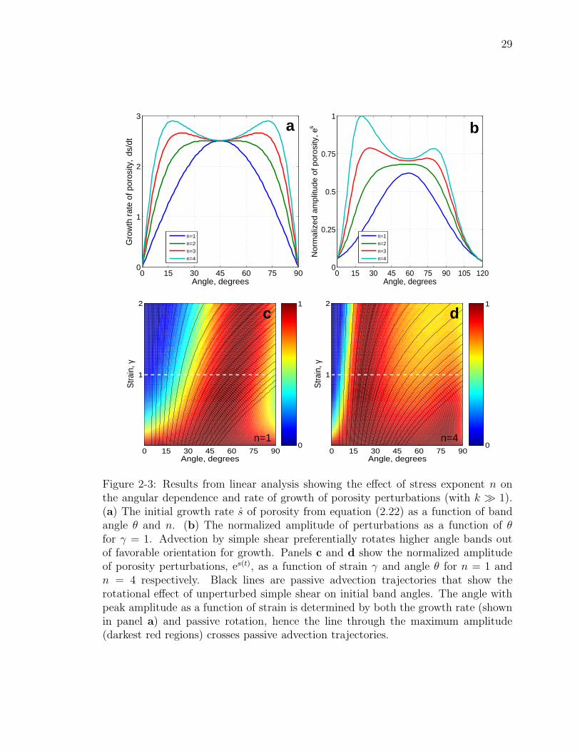
29
0 15 30 45 60 75 900
1
2
3
Angle, degrees
Gro
wth
rat
e of
por
osity
, ds
/dt
n=1
n=2
n=3
n=4
0 15 30 45 60 75 90 105 1200
0.25
0.5
0.75
1
Angle, degrees
No
rma
lize
d a
mp
litu
de
of p
oro
sity
, es
n=1
n=2
n=3
n=4
0 15 30 45 60 75 90
1
2
Angle, degrees
Stra
in, γ
0
1
0 15 30 45 60 75 90
1
2
Angle, degrees
Stra
in, γ
0
1
dc
a b
n=1 n=4
Figure 2-3: Results from linear analysis showing the effect of stress exponent n onthe angular dependence and rate of growth of porosity perturbations (with k 1).(a) The initial growth rate s of porosity from equation (2.22) as a function of bandangle θ and n. (b) The normalized amplitude of perturbations as a function of θfor γ = 1. Advection by simple shear preferentially rotates higher angle bands outof favorable orientation for growth. Panels c and d show the normalized amplitudeof porosity perturbations, es(t), as a function of strain γ and angle θ for n = 1 andn = 4 respectively. Black lines are passive advection trajectories that show therotational effect of unperturbed simple shear on initial band angles. The angle withpeak amplitude as a function of strain is determined by both the growth rate (shownin panel a) and passive rotation, hence the line through the maximum amplitude(darkest red regions) crosses passive advection trajectories.

30
0 15 30 45 60 75 90 105 120 135 150 165 180
1
4
Angle, degrees
n
0 15 30 45 60 75 90−4
−2
0
2
4
Angle, degrees
Ban
d−pa
ralle
l vel
ocity
per
turb
atio
n
n=1
n=2
n=3
n=4
a
b
Figure 2-4: Two descriptions of the perturbation velocity field from linear analysis.Panel a shows the relative sizes of the shear and volumetric components of the per-turbation flow field for n = 1, 4. The velocities for n = 4 are four times greater thanthose for n = 1 (as can be seen in panel b) but are scaled down to fit on the graph.It is evident from this panel that the volumetric component of strain goes to zeroat 0 and 90 while the shear component goes to zero at 45 and 135. The shearcomponent is always maximized at 0 and 90 to the shear plane. Panel b shows theshear component of the perturbation velocity field as a function of band angle and n.The amplitude of the perturbation scales with n. Curves for higher n show greaterenhancement of shear near 0 and 90 than the sine wave that represents n = 1.

31
increases with increasing strain to about 65 at γ = 2. For n = 4, there is initially a
symmetric bimodal distribution of amplitude at 15 and 75 but with increasing strain
the amplitude of low angle bands grows much more rapidly than that of high angle
bands. To validate these results requires numerical solutions of the full non-linear
equations.
2.2.2 Numerical solutions
The equations governing the two-phase aggregate are reviewed in the introduction of
this thesis. Some rearrangement puts them into the following form, convenient for
numerical solution,∂φ
∂t+ V · ∇φ = (1 − φ)∇·V, (2.23)
∇· V = ∇·kφ
µ∇P, (2.24)
∇P = ∇·[
η(
∇V + ∇VT)]
+ ∇
[(
ζ −2η
3
)
∇· V
]
, (2.25)
where φ is porosity, V is solid velocity, P is the dynamic pressure, kφ is permeability
(kφ ∝ φn), µ is the melt viscosity, η is the shear viscosity of the solid and ζ is
the bulk viscosity of the solid. Terms representing the buoyancy force and mass
transfer between solid and fluid are not included because they are negligible in the
experiments. The equations are discretized using a semi-implicit finite volume scheme
on a staggered mesh. The domain is periodic in the horizontal. On the top and
bottom boundaries the matrix velocity is required to satisfy V = ±U0 i + 0 j and
vertical gradients in pressure and porosity are required to equal zero.
Due to strong non-linearities and localization phenomena, computational solutions
to the full differential equations are challenging to obtain. However, we have made
significant progress using the Portable Extensible Toolkit for Scientific computation
(PETSc, (Knepley et al., 2006; Balay et al., 2001)) which provides a suite of tools
for the numerical solution of non-linear PDEs. The system of discrete non-linear
equations is solved using a Newton-Krylov-Schwarz method (Cai et al., 1997; Gropp
et al., 1998) with GMRES and an incomplete LU factorization preconditioner.

32
To investigate the effect of varying the stress-dependence of viscosity we ran 4
groups of simulations at n = 1, 2, 4, 6. Each group consisted of 4 model runs at
different grid resolutions from 50 to 80 cells per compaction length on a domain of
4x2 compaction lengths. Each run was initiated with 5 vol% background porosity
with 0.05 vol% white noise perturbation. The simulations were run until they failed
to converge, which typically occurred when inter-band porosities reached zero.
Output from a representative run with n = 6 is shown in Figure 2-1b–c at a
strain of γ = 2.79. The simulations are initiated with a small amount of random
noise added to a uniform background porosity field (<1% of φ0). Sharp gradients in
material properties due to localization cause convergence rates to degrade such that
we have not consistently been able to integrate the equations with high n beyond a
strain of about γ = 2.5
To quantify the band angle distributions in these simulations, histograms are
calculated by taking the 2D FFT of the porosity field and integrating the amplitude
response within 5 bins in band angle θ. Figure 2-1d shows the histogram derived
from Figure 2-1b. At each step of strain, similar histograms are produced from
ensembles of simulations with different seeds for initial noise. The power spectrum
of the initial noise field controls the wavelength of the emergent band pattern but
does not affect the angle. This is consistent with the prediction from linear analysis
that all perturbation wavelengths shorter than the compaction length grow. We have
typically initiated simulations with white noise. Figure 2-5a–b shows the evolution
of histograms with increasing strain for n = 1 and n = 4. The qualitative similarity
of these results to those shown in Figure 2-3c–d is striking. One salient difference is
that in simulations, even at small strain, high-angle bands do not grow.
Colored circles in Figure 2-5d chart the evolution of the preferred angle taken from
the histograms as a function of strain and n. Consistent with the linear analysis,
a more non-linear viscosity (higher n) results in a lower initial peak band angle.
Furthermore, peak band angle increases with strain for all n. However, this increase in
angle is not simply passive rotation by unperturbed shear flow. If it were, the symbols
would follow the passive advection trajectories shown by black lines in Figures 2-3c–d

33
Shear
str
ain
, γ
0 15 30 45 60 75 90
0.5
1.5
2.5
3.5
Angle, degrees
Simulation
n = 1n = 2n = 4n = 6 Experiment
φ0 = 0.02
φ0 = 0.06d
Angle, degrees0 15 30 45 60 75 90
0.5
1.5
2.5
3.5
0
1
c n=6
0 15 30 45 60 75 90
0.5
1.5
2.5
3.5
0
1
0 15 30 45 60 75 90
0.5
1.5
2.5
3.5
Shear
str
ain
, γ
ba n=1 n=4
(lin
ea
r a
naly
sis
)
(lin
ea
r a
naly
sis
)
Figure 2-5: Evolution of band angle in numerical simulations, experiments and linearanalysis. Panels a, b and c show the evolution of angle distribution averaged overfour simulations for n = 1, 4 and 6, respectively. In b and c simulations do notreach the maximum strains achieved in experiments and hence results from linearanalysis are used to extend them to γ = 3.6. For panels a–c, in the part of the plotderived from simulation results, each row at each step of strain represents a singlehistogram of the porosity field like the one in Figure 2-1d. These panels should becompared to Figure 2-3c and d. Panel d summarizes panels a, b and c as well assimulation results for n = 2 by plotting only the angle with maximum amplitudeas a function of strain. This represents the dominant band angle and is generallyconsistent with a visual estimate from the porosity field. Black symbols in all fourpanels represent mean band angles from independent experiments to different strain.Characteristics of porosity bands in experimental cross-sections were quantified byhand-measurement (not FFTs). A key question remains as to the behavior of the fullnon-linear calculations for high strain at n > 3.

34
and 2-5a–d and expressed analytically in equation (2.15). For example, a plane wave
initially oriented at 25 to the shear plane will rotate to 90 by a strain of γ ∼ 2.25
under passive advection. For n = 2, the peak band angle begins and remains at 25 to
a strain of about γ ∼ 1.5. It then appears to follow the passive advection trajectory
that initiated at about 16. Similar patterns are seen for higher n, however because
they initiate with lower peak band angle, the deviation from a passive advection
trajectory is more subtle. This behavior is also seen in the linear analysis (Figure
2-3c–d) and is the result of the interplay of instantaneous growth of bands in favored
orientation and the rotation of these bands out of this orientation by advection due
to simple shear.
2.3 Comparison with data
Data from experiments are shown by black symbols in Figure 2-5 and can be directly
compared to model results. Each point represents the mean of the distribution of
band angles measured in an individual experiment (see Figure 2-1a, d) (Holtzman
et al., 2003a). This data shows that the peak band angle is roughly constant at 10–
20 up to large strain. Up to a strain of about γ ∼ 2, the data are consistent with
simulations with n = 4 or 6. Unfortunately our current numerical techniques have not
been able to consistently take these simulations to higher strain. If linear analysis is
an accurate means for extending band angle evolution to higher strain than achieved
in simulations (Figure 2-5b–c) then results for n = 6 are most consistent with the
data. The open question is what mechanism is active in experiments at high strain
that maintains the low band angle.
Spiegelman (2003) suggests one mechanism for maintaining low angle in which
bands act as strain guides for matrix shear. These strain guides are assumed to
modify the solid flow field significantly from simple shear, reducing the amount of
rotation. Strain concentrations are observed in experiments (Holtzman et al., 2003a)
and in simulations (Figure 2-1b–c) where strain markers are offset across porosity
bands. However, comparison of strain markers to their positions predicted by simple

35
shear in Figure 2-1b–c shows that the deviation from simple shear is small.
Holtzman et al. (2005) propose another scenario in which a pumping mechanism
forces transfer of fluid from bands being rotated to higher angles to newly forming
bands at low angles. We note that in calculations reported here, some form of porosity
reorganization is constantly occurring, evidenced in Figure 2-5 by the observation
that the evolution of peak band angle does not follow passive advection trajectories.
Furthermore, an animation of calculations at large n (Movie S1) shows reconnection of
porosity bands, maintaining the dominance of those at low angle. This reorganization
is manifest in Figure 2-5b–c in that the standard deviation of the distribution does
not increase with strain.
2.4 Discussion
In all calculations some amount of porosity band reconnection is occurring. However
the dominant angle and standard deviation are ultimately controlled by the mag-
nitude of the strain rate dependence of viscosity (e.g. the size of n). Within the
context of the power-law viscosity used here, values of n ∼ 4 − 6 (Figure 2-5b–d)
are required to match observed band angles. These values are somewhat higher than
the values between 3 and 4 for partially molten aggregates undergoing dislocation
creep or dislocation-accommodated grain-boundary sliding inferred from uniaxial de-
formation experiments at small strains ≤ 25% (Hirth and Kohlstedt , 1995a,b). One
suggestion is that this discrepancy is due to the different deformation geometry be-
tween compression and shear configurations. An experimentally testable prediction
from our model is that deformation of a partially molten aggregate in simple shear
will have a larger strain rate dependence of viscosity than one deformed in uniaxial
compression. It should be emphasized, however, that the n that we predict is the
“material” n, valid at every point in the medium, and not the “effective” n that can
be calculated from stress–strain rate measurements taken through the course of an
evolving experimental run.
It should be noted that in these calculations, we assume a power-law viscosity

36
and treat n as a control parameter. The key feature of this rheology is the strain
rate-weakening mechanism that couples localized shear to the organization of poros-
ity bands. We suggest that any rheology that has a strain rate-weakening mechanism
would give similar results. Another example of such a rheology is plasticity, which
can also lead to strain localization (Rudnicki and Rice, 1975; Buck et al., 2005, e.g.).
Visco-plasticity can be approximated by a power-law stress dependence with large
n (Jellinek et al., 2005), however plastic rheologies typically prescribe an internal
friction angle which determines the angle of shear bands. A pleasing feature of our
calculations is that the band angle emerges naturally from the balance of two weak-
ening mechanisms with no apriori assumptions about angles.
2.5 Conclusion
In the analysis described here we have demonstrated how a non-Newtonian, strain
rate-weakening solid viscosity affects the dynamics of pattern formation in partially
molten aggregates. Our results show how the balance of stress and porosity-weakening
controls the angle at which porosity bands emerge and evolve in simulations. The
patterns developed in our calculations are quantitatively consistent with those ob-
served in experiments. There are, however, discrepancies between experiments and
calculations such as the aspect ratio and spacing of bands and the steep porosity gra-
dients at their edges. It is possible that models that use other strain rate dependent
rheologies can resolve these differences. On the other hand, these discrepancies may
point to physics that is missing from magma migration theory. Exploration of these
ideas provides opportunities and challenges for theorists and experimentalists.

37
Chapter 3
Mantle Flow and ThermalStructure in a KinematicSubduction Zone Model
3.1 Introduction
Models of the creeping solid flow of the mantle wedge and the associated arc thermal
structure are fundamental for understanding the context in which subduction zone
melting occurs. Two categories of these models exist and many investigators have
contributed to their development: “kinematic” models where the position of the slab
is fixed and drives a corner-flow in the adjacent wedge (Furukawa, 1993a; Kincaid
and Sacks , 1997; King , 2001; van Keken et al., 2002; Kelemen et al., 2002; Conder
et al., 2002b; Gerya and Yuen, 2003; van Keken, 2003a; Gutscher and Peacock , 2003;
Currie et al., 2004; Kincaid and Griffiths, 2004), and “dynamic models” in which
the slab’s position is determined by viscous stresses and buoyancy forces (Hager and
O’Connell , 1978; Becker et al., 1999; Billen and Gurnis, 2001; Gurnis et al., 2004;
Billen and Hirth, 2004). While the latter category of model is very important to our
understanding of the mechanics of subduction and its role in plate tectonics, a study
of arc magma genesis does not require computing a dynamically self-consistent slab
geometry. Recent models in the first category are broadly similar to each other and
emphasize the importance of including (at least) a temperature-dependent mantle
viscosity.

38
We have developed a kinematic model that employs a pressure, temperature and
stress dependent viscosity. This viscosity is consistent with experiments on dry, melt-
free mantle rocks (Karato and Wu, 1993; Hirth and Kohlstedt , 2003). As in simu-
lations with only temperature dependence of viscosity, our simulations show a more
focused mantle flow in the wedge corner, leading to a hotter mantle nose and slab
surface than in earlier constant viscosity flow/thermal models. Moreover, variable
viscosity solutions produce a component of solid upwelling. Output from representa-
tive calculations are shown in Figures 3-2 and 3-3. These results have been submitted
to a benchmark project for subduction zone thermal models (van Keken, 2003b) and
are nearly the same as results obtained by other approaches.
3.2 Governing equations and numerical solution
In the limit of zero porosity, no melting, and neglecting buoyancy forces the equations
of magma dynamics reduce to the incompressible Stokes equation and a steady-state
advection-diffusion equation for potential temperature θ,
∇P = ∇·[
η(
∇V + ∇VT)]
, s.t. ∇· V = 0, (3.1)
V · ∇θ = κ∇2θ, (3.2)
where V is the solid velocity, P is the dynamic pressure and κ is the thermal diffusivity.
The true temperature is given by
T = T0 θ exp
(
αg
cPz
)
(3.3)
where T0 is a reference temperature, α is the thermal expansivity, g represents gravity,
cP is the specific heat and z is the depth.
The dynamic viscosity in equation (3.1) can be chosen as a constant (isoviscous),
diffusion creep (pressure and temperature dependent) or combined diffusion/dislocation
creep (non-Newtonian pressure, temperature and stress dependent). For the latter,

39
diffusion and dislocation viscosities are combined to give an effective viscosity,
ηeff =2
η−1disl + η−1
difn
. (3.4)
Independently, the dislocation and diffusion creep viscosities are given by
ηdisl,difn = A0 exp
(
E∗ + PV ∗
nRT
)
ε1−n
n
II (3.5)
where A0, E∗, V ∗, and n are material constants that are different for diffusion and
dislocation creep (their values are given in Table 3.1). R is the universal gas constant,
P is the total pressure (approximately equal to the lithostatic pressure), T is the
absolute temperature and εII is the second invariant of the strain-rate tensor. For
numerical stability, viscosity is truncated at 1024 Pa-s, which is sufficient to preserve
the rigid behavior of the cold lithosphere [van Keken, pers. comm. 2003].
Equations (3.1), (3.2) and the boundary conditions are discretized using a finite
volume approach on a fully staggered grid and solved within the PETSc framework
using a Newton-Krylov-Schwarz method (Cai et al., 1997; Gropp et al., 1998), typi-
cally GMRES with an ILU preconditioner (see chapter 1 for details). The software
and application are described in detail by Knepley et al. (2006). The computational
domain is divided into subdomains where different equations for the velocity are
solved. A schematic layout is shown in Figure 3-1. Below the slab surface, velocity is
prescribed to be equal to the convergence rate resolved into its vertical and horizontal
components, according to a prescribed slab dip. The crustal velocity is prescribed to
be zero and in the wedge the velocity is the solution of equation (3.1). The depth of
the base of the crust is independent of the fault depth, however the fault depth can
be no smaller than the crustal thickness. Cells in the wedge that border the fault
“see” a velocity of zero across the fault. This would be better implemented with a
stress-free boundary condition on the fault (or with a set of weak, visco-plastic cells).
With a full non-Newtonian viscosity, this system is highly ill-conditioned, even
singular, unless a very good initial guess at the solution is given. Because vari-

40
Parameter Value ValueName Diffusion Creep Dislocation Creep UnitsPrefactor, A0 1.8 × 10⁷ 2.9 × 10⁴ Pa secActivation energy, E∗ 375 530 kJ mol−1
Activation volume, V ∗ 5 × 10⁻³ 14 × 10−6 m3 mol−1
Stress exponent, n 1 3.5
Table 3.1: Empirically determined parameters for diffusion and dislocation creep(Karato and Wu, 1993; Hirth and Kohlstedt , 2003) used in equation (3.5).
η=η(P,T,V)No Slip
V
Subducting slab
No Slip
Crust
Stre
ss f
ree
Dislocation and diffusion creepMantle
slab
Distance from trench
Dep
th
Zero velocity
fault
Figure 3-1: A schematic diagram of the computational domain showing the slab, crustand wedge subdomains.

41
able viscosity solutions are not available analytically we have adopted a continuation
method to gradually approach the full variation in viscosity from initially constant
viscosity. Specifically, we modify the normalized viscosity
η → ηβ (3.6)
where β is the continuation variable and is constrained to fall between zero and one.
For each simulation, a full solution is first obtained with β = 0 (constant viscosity).
This solution becomes the initial guess for the next solution step and β is increased
by a constant amount. Iteration leads eventually to a solution where β = 1, which
represents full variation of viscosity. If a step fails to converge, β is reduced by a
set fraction and the solve is repeated. A typical solution with full viscosity variation
requires 10-15 continuation steps, depending on other parameters such as slab dip.
This method can be very slow (100-1000 times longer than to obtain the solution for
a constant viscosity) but has proved robust.
3.3 Results
A set of representative results from a simulation with full diffusion/dislocation creep
viscosity and 45 slab dip is given in Figure 3-2. The viscosity field for this simulation
is shown in Figure 3-3. It is evident from Figure 3-2a that the pressure gradients very
close to the singularity at the base of the fault are large but that these gradients do
not extend far into the wedge. Increased grid resolution would possibly lead to a large
negative pressure spike near the singularity but would not resolve any more fine-scale
structure. Diffusive cooling of the lithosphere from above produces a thick thermal
boundary layer that is too viscous to flow. Slab-wedge coupling, however, drags the
mantle constantly downward from the wedge corner and requires a counterflow from
the wedge to satisfy incompressibility. This flow is constrained by the lithosphere
above and the slab below and is hence highly localized relative to isoviscous corner
flow, as is evident in Figures 3-2c–d and 3-4a–c. Furthermore, the counterflow has a

42
SCALED PRESSURE
30 40 50 60 70
30
40
50
60
70−100
−80
−60
−40
−20
POTENTIAL TEMPERATURE, °C
0 100 200 3000
50
100
150
200
250
3000
200
400
600
800
1000
1200
VERTICAL VELOCITY, cm/yr
0 100 200 3000
50
100
150
200
250
300−2
−1
0
1
2
3
4
5
HORIZONTAL VELOCITY, cm/yr
0 100 200 3000
50
100
150
200
250
300−5
0
5
(a) (b)
(c) (d)
Figure 3-2: Representative results from the numerical solution of equations with fulldiffusion/dislocation creep viscosity, slab dip of 45, convergence rate of 8 cm/year,crustal thickness of 35 km and a fault depth of 50 km. Depths and distance fromthe trench are given in km on the y and x axes respectively. The domain is 350 kmwide by 300 km deep and the resolution is < 2 km in both directions. The viscosityfield is shown in Figure 3-3. (a) Dimensionless pressure. Note that this panel ison a different scale than the others; The pressures are large and non-zero only veryclose to the base of the fault. (b) Potential temperature in degrees centigrade. Notethe relatively high temperatures near the wedge corner. (c) Vertical component ofthe velocity field in cm/yr. Note the strong upwelling toward the wedge corner. (d)Horizontal velocity in cm/yr.

43
strong vertical component with important implications for adiabatic melt generation.
As shown in Figure 3-4, the temperature field difference between isoviscous flow
and pressure/temperature dependent flow is much greater than the difference between
temperature/pressure dependent flow and non-Newtonian temperature/pressure de-
pendent flow. Isoviscous models allow cold mantle to flow as readily as hot mantle
resulting in advection of colder rock along the base of the crust, into the corner and
onto the slab surface. Giving viscosity a temperature dependence prevents this by
requiring the thermal lithosphere to be resistant to flow. The stress dependence of
viscosity actually lowers the temperature of the nose of the wedge because it allows
for reduced viscosity of cold, high-stress lithosphere, making it possible to advect
some colder rock into the wedge corner.
Inspection of the flow fields in Figure 3-2c–d reveals that the strong counterflow
is directed toward the bottom of the fault where the slab-wedge interface is fully
coupled. The depth of this point, the base of the interplate fault, is a critical and
poorly constrained parameter in these simulations. Conder (2005) makes a case for
assigning its position dynamically based on a yield stress criterion. The depth of the
fault controls the distance to the surface to which hot mantle solid will penetrate.
Besides the obvious effects on surface heat flow, hot shallow mantle will tend to melt
extensively and this would contribute to the magma budget of the arc. Seismicity on
the plate interface extends to about 35 km in most arcs and this depth provides a
lower bound on the slab-mantle coupling depth. Water release from the slab could
hydrate the mantle at the slab–wedge interface and cause the formation of a narrow,
fault-like shear zone that would aseismically extend the fault deeper into the mantle.
Such an extension of the fault would reduce the advection of cold mantle rock out of
the nose of wedge and hence stabilize the fault’s depth extent.

44
LOG10
VISCOSITY (Pa−s)
0 100 200 300
0
50
100
150
200
250
30019
20
21
22
23
24
Figure 3-3: The log10 of viscosity field from the same simulation as shown in Figure3-2. Depths and distance from the trench are given in km on the y and x axesrespectively. The effect of the stress dependence of viscosity can be seen most clearlyin the diagonal band of dark blue sub-parallel to the slab where mantle shear isstrongest.
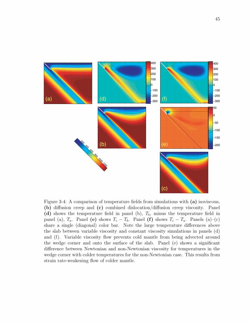
45
−300
−200
−100
0
100
200
300
400
−200
−150
−100
−50
0
50
−300
−200
−100
0
100
200
300
400
200400
600800
10001200
(a)
(b)
(c)
(d)
(e)
(f)
Figure 3-4: A comparison of temperature fields from simulations with (a) isoviscous,(b) diffusion creep and (c) combined dislocation/diffusion creep viscosity. Panel(d) shows the temperature field in panel (b), Tb, minus the temperature field inpanel (a), Ta. Panel (e) shows Tc − Tb. Panel (f) shows Tc − Ta. Panels (a)–(c)share a single (diagonal) color bar. Note the large temperature differences abovethe slab between variable viscosity and constant viscosity simulations in panels (d)and (f). Variable viscosity flow prevents cold mantle from being advected aroundthe wedge corner and onto the surface of the slab. Panel (e) shows a significantdifference between Newtonian and non-Newtonian viscosity for temperatures in thewedge corner with colder temperatures for the non-Newtonian case. This results fromstrain rate-weakening flow of colder mantle.

46
3.4 Discussion
3.4.1 Magma genesis in subduction zones
There are three general, independent mechanisms for the generation of molten rock in
subduction zones: reactive hydrous melting of the mantle, adiabatic decompression
melting of the mantle, and hydrous melting of the downwelling slab’s crust and/or
sediments. While the calculations described in this chapter do not explicitly predict
melting by any of these mechanisms, thermal structure and mantle flow form the
context for all melting that occurs in a subduction zones. Hence the simulations
described in this chapter can be interpreted in terms of the constraints that they
place on melting (or lack thereof).
Hydrous reactive mantle melting. Hydrous reactive melting of mantle rock is
generally expected to the the major source of arc volcanic material. Arc magmas
show a range of volatile contents, from considerably higher than MORB and OIB
(e.g. & 3wt% H2O in primitive arc basalts) (e.g. Gill , 1981; Stolper and Newman,
1994; Sisson and Layne, 1993; Sobolev and Chaussidon, 1996; Plank et al., 2004)
down to near anhydrous concentrations in some primitive arc basalts (e.g. Sisson
and Bronto, 1998). This water in arc lavas is carried to depth by hydrous minerals
in the subducting slab and released as a silicate rich fluid in metamorphic reactions
(Schmidt and Poli , 1998; Forneris and Holloway , 2003; Manning , 2004). As the
fluid rises through the mantle it experiences increasing temperature and decreasing
pressure with height and hence a rapid increase in the solubility of silicate components
leading to “dissolution” of the mantle matrix by the fluid. Katz and Spiegelman (2004)
showed that this process leads to channelized flux of hydrous magma in a model of
hydrous reactive melt transport. While this process requires only an inverted thermal
gradient above the slab (which is present in all thermal structure models), the details
of fluid reaction distribution and melt flow trajectories will depend heavily on the
thermal structure. The details of this process are considered in chapter 5.

47
Adiabatic decompression mantle melting. Anhydrous lavas are found among
volcanics at some subduction zones; these lavas appear to be the product of decom-
pression melting, much like mid-ocean ridge lavas. Sisson and Bronto (1998) showed
an example of this from Galunggung, Indonesia. Kelley et al. (2004) later showed
that the lavas from this region form two groups with respect to water content, one
clearly the product of hydrous melting and the other nominally anhydrous. Flow
simulations described here and elsewhere (e.g. van Keken et al., 2002; Kelemen et al.,
2002; Conder et al., 2002b) demonstrate that passive upwelling of mantle flow is a ro-
bust prediction of calculations with temperature dependent viscosity. Calculations by
Gerya and Yuen (2003) have shown that active upwelling due to compositional buoy-
ancy may produce decompression melts however these melts are unlikely to have the
composition of MORB because dry mantle peridotite is not compositionally buoyant.
Slab melting. Slab melting has long been invoked by petrologists to explain the
geochemical signature of arc volcanic rocks called Adakites (Kay , 1978; Kelemen
et al., 1990; Kay et al., 1993; Martin et al., 2005). The debate on whether slab melting
occurs today has focused on whether kinematic simulations of arc thermal structure
can produce slab-surface temperatures hot enough for slab melting (Peacock , 1990).
While isoviscous models typically have slabs that are too cold to melt, Kelemen et al.
(2002) showed that slab surface temperatures in a model with temperature dependent
viscosity are significantly hotter and may be high enough to cause melting. This work
also considered thermal constraints provided by heat flow and observed metamorphic
facies and concluded that they are inconsistent with isoviscous models but agree with
variable viscosity simulations. While the addition of stress dependence of viscosity
from the dislocation creep mechanism may cool the corner relative to diffusion creep
viscosity, the slab surface remains at about the same temperature, as shown in Figure
3-4e. A comparison of slab surface temperatures from simulations presented here is
given in Figure 3-5. These curves show hotter temperatures than the those calculated
by Kelemen et al. (2002) although they are similar to curves obtained by van Keken
et al. (2002). In fact, curves representing variable viscosity simulations cross the

48
fluid-saturated basalt solidi given by Kelemen et al. (2002) at about 3.5 GPa. These
simulations indicate that slab melting may contribute to magma genesis in arcs.
3.4.2 Magma focusing in subduction zones
Spiegelman and McKenzie (1987) investigated pressure gradients caused by isoviscous
corner flow as a mechanism for melt focusing in arcs and ridges. For fluid flow to devi-
ate from vertical percolation driven by buoyancy, horizontal pressure gradients must
be approximately equal to or greater than buoyancy. As Spiegelman and McKenzie
(1987) showed, for reasonable mantle porosities and crustal production rates, vis-
cosities of ∼ 1021 are required in an isoviscous corner-flow model. Variable viscosity
models described here (see Figure 3-3) demonstrate that experimentally constrained
viscosities may be much lower than this in the mantle wedge beneath subduction
zones. Sparks and Parmentier (1991) argued that these low viscosities would reduce
pressure gradient forces well below the level of the buoyancy force acting on the melt
and hence preclude pressure-driven focusing of melt into the wedge corner.
The results of fluid flow calculations similar to that of Spiegelman and McKenzie
(1987) are shown by streamlines in Figure 3-6. Not surprisingly, constant 1021 Pa-s
viscosity corner-flow (panels a and b) has significant flow focusing. The fluid flow
lines in a simulation with combined diffusion/dislocation creep viscosity (panels e
and f) are vertical where viscosities are low, except in the wedge corner above the
the interplate fault. Here strain is very large and produces strong pressure gradients.
This is different from the case where viscosity is temperature and pressure dependent
only, shown in Figure 3-6c–d. Here viscosity is higher in the mantle wedge, coupling
stress more efficiently between the slab and the lithosphere and driving a broader
convergence of melt streamlines. Small amounts of deformation in the cold lithosphere
and in the layer of cold mantle accreted to the slab surface produce strong pressure
gradients that draw in fluid in horizontally from a large region of the wedge. It
is interesting to note that although the viscosity fields of diffusion and combined
diffusion–dislocation creep are nearly identical, there is a large difference in the fluid
flow fields in each case, predicted by this model. All else being equal (or nearly so),

49
0 100 200 300 400 500 600 700 800 900
0
50
100
150
200
Temperature, °C
Dep
th, k
m
IsoviscousDiffusion CreepDislocation/Diffusion Creep
0 100 200 300 400 500 600 700 800 900
0
50
100
150
200
Temperature, °C
Dep
th, k
m
IsoviscousDiffusion CreepDislocation/Diffusion Creep
0.0
1.5
3.0
4.5
6.1
Pre
ssur
e, G
Pa
Figure 3-5: Slab surface temperature profiles for simulations shown in Figure 3-4a–c.These simulations all have a mantle potential temperature of 1300 C. The isoviscousflow model produces a slab surface temperature that is much lower than that ofNewtonian and non-Newtonian temperature dependent viscosities.

50
fluid flow paths or distribution might provide a diagnostic for the style of deformation
active in subduction zones.
The strongly sloping thermal boundary at the base of the lithosphere in subduction
zone calculations may provide another means for focusing magma toward the corner.
Sparks and Parmentier (1991) proposed a focusing mechanism for ridges in which
rising magma encounters a permeability barrier at the base of the lithosphere where
colder temperatures cause freezing and the reduction of porosity. They show that melt
migration along this sloping boundary layer is directed toward the ridge and delivers
sufficient melt to account for the observed crustal thickness. Spiegelman (1993a),
Magde and Sparks (1997) and Ghods and Arkani-Hamed (2000) later confirmed these
results in two and three dimensions although they also showed that the process is less
efficient that previously assumed. The same mechanism may affect the trajectory of
magma as it rises through the mantle beneath an arc. One question this raises is
whether the magma would rise all the way to the hot nose of the wedge or whether
it would traverse the cold boundary later at some point “downslope” from the nose.
Arc magmatism is localized in a volcanic front that is invariably 120 ± 40 km
above the earthquakes in the slab (e.g. Gill , 1981; Tatsumi , 1986; Jarrard , 1986).
Recent work by England et al. (2004) suggests that the depth to earthquakes is anti-
correlated with slab convergence rate and dip-angle, but otherwise insensitive to most
subduction parameters. This trend is consistent with thermal calculations where the
penetration of the nose of hot mantle rock into the wedge corner increases with
increasing convergence rate and slab dip (England and Wilkins , 2000). A comparison
of two possible indicators of volcano position with data from England et al. (2004) is
shown in Figure 3-7. Both of these, the position of the maximum degree of melting1
Fmax and the position of the “nose” of the 1225C isotherm, vary with convergence
rate (and slab dip) in the same way according to simulations. Hence it is possible
that neither, one or both contribute to determining the depth of the slab beneath
the volcanic arc. The important point here is that the observations by England et al.
1The maximum degree of melting is computed by using the parameterization described in chapter4 and assuming a constant bulk water content of 0.01 over the whole domain.
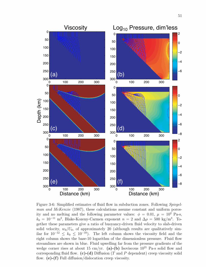
51
0 100 200 300
0
50
100
150
200
250
300
−6
−4
−2
0
2
0 100 200 300
0
50
100
150
200
250
300 −8
−6
−4
−2
0
0 100 200 300
0
50
100
150
200
250
300−8
−6
−4
−2
0
2
0 100 200 300
0
50
100
150
200
250
300
0 100 200 300
0
50
100
150
200
250
300
0 100 200 300
0
50
100
150
200
250
300
(a)
(f)(e)
(d)(c)
(b)
Viscosity Log10 Pressure, dimʼless
Depth (km)
Distance (km)Distance (km)
Figure 3-6: Simplified estimates of fluid flow in subduction zones. Following Spiegel-man and McKenzie (1987), these calculations assume constant and uniform poros-ity and no melting and the following parameter values: φ = 0.01, µ = 102 Pa-s,k0 = 10−11 m2, Blake-Kozeny-Carmen exponent n = 2 and ∆ρ = 500 kg/m3. To-gether these parameters give a ratio of buoyancy-driven fluid velocity to slab-drivensolid velocity, w0/U0, of approximately 20 (although results are qualitatively sim-ilar for 10−12 ≤ k0 ≤ 10−10). The left column shows the viscosity field and theright column shows the base-10 logarithm of the dimensionless pressure. Fluid flowstreamlines are shown in blue. Fluid upwelling far from the pressure gradients of thewedge corner rises at about 15 cm/yr. (a)-(b) Isoviscous 1021 Pa-s solid flow andcorresponding fluid flow. (c)-(d) Diffusion (T and P dependent) creep viscosity solidflow. (e)-(f) Full diffusion/dislocation creep viscosity.

52
(2004) are consistent with predictions from variable viscosity simulation of arc thermal
structure.
3.5 Conclusions
A kinematic solid flow and thermal structure simulation is a critical component in
any model of magma genesis and transport in subduction zones because it forms the
context in which melting occurs. Recent work by Kelemen et al. (2002) has demon-
strated the deficiencies associated with isoviscous models and has emphasized the
importance of employing a viscosity that is at least temperature dependent. The
simulations presented here use temperature, pressure and stress dependent viscos-
ity that approximates the empirically derived flow laws for diffusion and dislocation
creep of olivine. We show, however, that the difference in thermal structure between
a Newtonian temperature dependent viscosity and a non-Newtonian one is small rel-
ative to the difference between isoviscous and variable viscosity simulations. The
computational cost for non-Newtonian viscosity is at least a factor of five (more in
some cases) greater than for Newtonian viscosity. On the other hand, calculations of
melt flow in response to pressure gradients in this chapter and in chapter 2 show that
melt organization is strongly dependent on the stress exponent of solid viscosity.
Simulations described here are consistent with the presence of three mechanisms of
melting beneath arcs. Hydrous reactive melting is plausible in all solid flow and ther-
mal structure models of subduction zones. Decompression melting and slab/sediment
melting, however, depend on features of the simulations that are not present in iso-
viscous models. Variable viscosity simulations predict the presence of significant up-
welling in sub-arc mantle flow and slab surface temperatures that cross the hydrous
basalt solidus. Explicit melting and melt transport calculations are needed to resolve
the contributions of each of these three melting mechanisms.
It remains a challenge to model both the slab-driven solid flow field and a consis-
tent reactive fluid flow field simultaneously. With the added complexity of porosity
dependent viscosity and reactive localization instabilities in the physics of porous

53
0 02 04 06 08 00106
08
001
021
041
061
081
002 03°
04°
05°
06°
07°
ataddepth
to s
lab a
t F
max, km
0 02 04 06 08 00106
07
08
09
001
011
021
031
041
051
depth
to s
lab a
t nose o
f 1225
° isoth
erm
, km
(nis V δ ry/mm ,)
03°
04°
05°
06°
07°
atad
(a)
(b)
Figure 3-7: A comparison of two possible proxies for volcano position derived fromnumerical simulations with data from England et al. (2004). (a) Depth from thevolcanic arc to the slab assuming that the arc is directly above the location of themaximum degree of melting, Fmax. Fmax is computed using the parameterizationdescribed in chapter 4 assuming a constant bulk water content everywhere in thedomain. (b) Depth from the volcanic arc to the slab assuming that the arc is directlyabove the “nose” of the 1225C isotherm. The nose is the point on the isotherm withthe shortest horizontal distance to the trench. Its position may provide a proxy forthe limit to lateral melt transport toward the wedge corner.

54
magmatic flow, such models will require significant computational power as well as
grid and solver technologies more advanced than those used here. Nonetheless, these
simulations will have solid flow field and thermal structure calculations at their core.

55
Chapter 4
A New Parameterization ofHydrous Mantle Melting
Richard F. Katz, Marc Spiegelman and Charles Langmuir
Geochem. Geophys. Geosyst. 4(9):1073, 2003
Copyright by the American Geophysical Union
Abstract
Modeling of melt formation and transport in all tectonic settings requires the inclusionof water, since water has large effects on mantle solidi as well as physical propertiesof liquids. To facilitate the inclusion of water in melting models this paper presents anew parameterization for melt fraction as a function of pressure, temperature, watercontent and modal cpx, based on knowledge gained from recent advances in thefields of thermodynamic modeling as well as experimental investigations of peridotitemelting and hydrous equilibria. The parameterization is computationally efficient andcan be modified easily as better experimental data become available. We compare itto other published parameterizations and test it in simple calculations of adiabaticdecompression melting (mid-ocean ridge) and hydrous melting (subduction zone).
4.1 Introduction
Magma genesis and transport in subduction zones influence large scale chemical cy-
cling in the mantle and provide the crucial link between mantle dynamics and geo-
chemical signals observed in island arcs. Nevertheless, many aspects of these processes
are still poorly understood. The challenge remains to integrate theory, experiment
and observation into a consistent framework that permits inferences on subduction
zone chemistry and dynamics from available observations. Quantitative models of

56
subduction zones provide such a framework. To consistently model both solid and
fluid/melt processes, however, requires an accurate and computationally efficient pa-
rameterization of mantle melting that includes the effects of significant amounts of
water. We present here a new parameterization that, while remaining mathematically
simple, succeeds in capturing the important features of the behavior of this complex
thermodynamic system.
While a full thermodynamically consistent treatment of melting might be pre-
ferred, current equilibrium thermodynamic models such as MELTS and pMELTS
(Ghiorso, 1994; Ghiorso and Sack , 1995; Ghiorso et al., 2002; Asimow and Stolper ,
1999) remain too computationally expensive for large time-dependent 2-D calculations
(although see Tirone and Ganguly , 2002) that are necessary to create quantitative
models applicable to ridges and convergent margins. Furthermore, these models do
not cover the full range of pressure, temperature and composition conditions relevant
to subduction zones. Thus melting parameterizations are a useful way to incorporate
melting into tectonic models, and these parameterizations also have the advantage
that they often better reproduce existing experimental data.
Thermodynamic constraints on such models, however, are also important. As we
show, current experimental data for wet melting is sparse and experimental data for
dry melting shows a large amount of scatter, even on nominally identical samples (see
also Hirschmann (2000)). In order to make progress, here we take an approach that
incorporates many of the theoretical concepts from thermodynamic models and and
also calibrates them against the current experimental database.
Other workers have produced various parameterizations (McKenzie and Bickle,
1988; Davies and Bickle, 1991; Langmuir et al., 1992; Kinzler and Grove, 1992; Jha
et al., 1994; Iwamori et al., 1995; Iwamori , 1997; Kinzler , 1997); the discussion below
presents a comparison of the different models. Overall, many of the parameterizations
are qualitatively similar to each other with different biases in different parts of pa-
rameter space. Further progress in refining parametric melting functions will require
either additional experiments or concerted efforts to better quantify the uncertainty
in the experimental database.

57
4.1.1 Basic structure of the parameterization
Our parameterization is of the form F = f(P, T,XH2O,Mcpx) where F is the weight
fraction of melt present, P is the pressure in GPa, T is the temperature in degrees
Celsius, XH2O is weight fraction of water dissolved in the melt and Mcpx is the modal
cpx of the unmelted (or residual) peridotite. This parameterization incorporates the
following concepts and principles:
1. The isobaric melting function, F should be monotonically increasing, concave
upward, with isobaric productivity, ∂F/∂T |P,XH2Oincreasing as a function of T
(Hirschmann et al., 1999), as long as the phase assemblage remains constant.
We utilize this constraint despite the fact that existing experimental data do
not clearly show the effect.
2. F (T ) should be kinked when major phases are exhausted from the residue, such
as when F = Fcpx−out. In other words, productivity should decrease discontin-
uously at this point and then rise as it did for melting in the low-F regime
(Hirschmann et al., 1999).
3. For a peridotite with fertile mineral compositions, the melt reaction coeffi-
cient of cpx is a function of pressure only. Thus, Fcpx−out can be predicted
given the modal cpx of the peridotite being melted and the pressure of melt-
ing. (Pickering-Witter and Johnston, 2000; Longhi , 2002; Walter , 1998; Walter
et al., 1995)
4. Addition of water to a peridotite system should monotonically increase F at
constant T and P . F (XH2O) at constant temperature and pressure should be
an approximately linear increasing function for small XbulkH2O. Furthermore, the
slope should increase with increasing temperature, (Hirschmann et al., 1999;
Hirose and Kawamoto, 1995; Hirose, 1997; Gaetani and Grove, 1998)
∂F
∂XbulkH2O
∣
∣
∣
∣
P,T
= c(T ), c > 0. (4.1)

58
5. Addition of water to a peridotite system should lower the solidus (except at
atmospheric pressure) in proportion to XH2O. This seems to be uniform with
P (Burnham, 1979). It should also lower the liquidus of the solid. However,
for melt fractions near one and modest bulk water content, the weight percent
dissolved water at the liquidus is small because it is diluted by silicate melt.
Thus the liquidus is not lowered substantially, except by extreme water contents.
6. Assuming, after Michael (1995) and Asimow and Langmuir (2003), that water
may be treated as an incompatible element, addition of water to the system
depresses the solidus until the melt becomes saturated. Of course the amount
of water at saturation is strongly dependent on pressure. Because the amount
of water in the liquid decreases progressively as melting proceeds, the influence
of water progressively decreases, and hence productivity above the wet solidus
remains low until a temperature near the dry solidus is reached (Hirth and
Kohlstedt , 1996; Hirschmann et al., 1999).
7. Experiments show that XsaturatedH2O
is zero at atmospheric pressure, about 13 wt%
at 1 GPa and continues to rise with increasing pressure. (Dixon et al., 1995;
Mysen and Wheeler , 2000)
4.2 Mathematical Formulation
4.2.1 Anhydrous Melting
Fcpx is the degree of melting expected by equilibrium batch melting prior to the
exhaustion of cpx. We parameterize it as a power-law of the rescaled temperature T ′.
Fcpx(T′) = [T ′(T, P )]
β1 , (4.2)

59
where
T ′(T, P ) =T − Tsolidus(P )
T lherzliquidus(P ) − Tsolidus(P )
. (4.3)
is the fractional distance in temperature between the solidus and “lherzolite liquidus”
(defined below). Here T is the temperature in Kelvin and the pressure dependence is
hidden in Tsolidus and T lherzliquidus. Using the form suggested by Hirschmann (2000),
Tsolidus = A1 + A2P + A3P2, (4.4)
T lherzliquidus = B1 +B2P +B3P
2, (4.5)
for pressure in GPa (figure 4-1). The “lherzolite liquidus,” T lherzliquidus, in Eq. (4.2) is
introduced as a means for creating a kinked melting function. It can be conceptualized
as the temperature that the liquidus would have if melting continued according to
Eq. (4.2) to F = 1, i.e. with cpx remaining in the residue. Cpx-out occurs at
some F < 1, and at this point there is a discontinuous change in the productivity
of the system. For simplicity, we do not consider the effect on melt productivity of
the exhaustion of the aluminous phase, although Walter (1998) has shown that the
exhaustion of garnet occurs before the exhaustion of cpx at pressures between 2 and 4
GPa. Furthermore, we ignore the loss of opx from the residue as this typically occurs
at melt fractions beyond what we expect in an arc setting (thus we do not define a
“hartzburgite liquidus”). For a closed (batch) system,
Fcpx−out =Mcpx
Rcpx(P ). (4.6)
Mcpx is the weight fraction of cpx in the solid peridotite being isobarically melted.
Rcpx is the reaction coefficient for cpx in the melting reaction. Following experimental
results of Longhi (2002), Walter (1998), Walter et al. (1995) and Pickering-Witter
and Johnston (2000), we give this reaction coefficient a pressure dependence of the
form
Rcpx(P ) = r0 + r1P. (4.7)

60
There is evidence from Walter (1998) and Kelemen et al. (1992) that Rcpx reaches a
maximum at about 3.5 GPa and decreases at higher pressures (in the garnet stability
field). For simplicity, we neglect this effect but it may need to be reconsidered for
applications where significant melting occurs at pressures greater than 3.5 GPa.
For F > Fcpx−out, the melting reaction changes to consume mostly opx and the
melting function is:
Fopx(T ) = Fcpx−out + (1 − Fcpx−out)
[
T − Tcpx−out
Tliquidus − Tcpx−out
]β2
, (4.8)
where
Tcpx−out = F1
β1cpx−out
(
T lherzliquidus − Tsolidus
)
+ Tsolidus (4.9)
and Tliquidus is the true liquidus of the model peridotite system (Figure 4-1),
Tliquidus = C1 + C2P + C3P2. (4.10)
The shape of the overall melting function at different pressures is shown in Figure
4-2. As mentioned in the introduction, ∂2F/∂T 2|P,XH2O> 0 for the isobaric melting
curves and they are kinked at cpx out. The pressure dependence of Rcpx is evident in
the melt fraction at which cpx is exhausted from the residue.
4.2.2 Hydrous Melting Extension
This parameterization of dry melting can be extended to include systems where the
dissolved water fraction in the melt in weight fraction, XH2O, is specified (the weight
fraction of bulk water is written as XbulkH2O
). Specifically, the changes are the following:
Tsolidus(P ) → Tsolidus(P ) − ∆T (XH2O) (4.11)
T lherzliquidus(P ) → T lherz
liquidus(P ) − ∆T (XH2O) (4.12)
Tliquidus(P ) → Tliquidus(P ) − ∆T (XH2O) (4.13)

61
1200 1400 1600 1800 2000
0
1
2
3
4
5
6
7
8
Pre
ssur
e, G
Pa
Temperature, °C
Anhydrous pseudo−phase diagram
SolidusLherzolite liquidusLiquidusHirschmann 2000 solidusLangmuir 92 solidusMcKenzie & Bickle solidus
Figure 4-1: The anhydrous solidus, lherzolite liquidus (see text) and liquidus. Alsoshown, for comparison, the anhydrous solidi of Hirschmann (2000), Langmuir et al.(1992) and McKenzie and Bickle (1988).

62
1000 1200 1400 1600 1800 20000
0.2
0.4
0.6
0.8
1
Temperature, °C
Mel
t fra
ctio
n, F
Isothermal (1 GPa) anhydrous melting
0 GPa1 GPa2 GPa3 GPa
Figure 4-2: Isobaric anhydrous melting curves at different pressures with modal cpxof the unmelted rock at 15 wt%. For a comparison of these calculations to data, seeFigure 4-6.

63
where ∆T (XH2O) is the temperature decrease in the solidus caused by a water content
XH2O in the melt. This function, the same for the liquidus, lherzolite liquidus and
solidus, may take a variety of forms as long as they satisfy:
∆T (XH2O = 0) = 0, (4.14)
∆T (XH2O ≥ XsatH2O) = ∆T (Xsat
H2O). (4.15)
where XsatH2O
(P ) is the weight percent of water in a completely saturated melt, which is
principally a function of pressure. The criterion stated in equation (4.15) is necessary
because of the way that we handle a free vapor phase. For computational simplicity,
water present beyond the saturation of the melt is not computed as a separate vapor
phase, it is accounted for as a part of the fluid phase which also includes the saturated
silicate melt. The thermodynamic properties (e.g. liquidus) of the silicate melt are
unaffected by water content beyond saturation. The utility of this simplification is
that it permits the use of a standard two-phase fluid mechanical formulation for melt
transportMcKenzie (1984); Spiegelman (1993a).
The speciation of water dissolved in silicate melt has been a subject of debate (for
a summary and references, see Withers et al. (1999)). Stolper (1989) and Ihinger et al.
(1999) have reported that at temperatures near the water saturated rhyolite solidus,
the first 1-2 wt% water dissolved into the melt exists mostly as hydroxyl ions (al-
though see Mosenfelder et al. (2002)). For higher dissolved water contents, molecular
water becomes the dominant species, however, increasing temperature diminishes the
proportion of molecular water. The depolymerizing effect of hydroxyl ions on silicate
melt exceeds that of molecular water because of its non-zero charge; depolymerization
of the melt increases its entropy, stabilizing it at lower temperatures. Thus we choose
a form for ∆T (XH2O) that has a steep slope at low water contents and grows more
slowly after that. This form is consistent with the data shown in figure 4-8a, within
their uncertainties.
∆T (XH2O) = KXγH2O, 0 < γ < 1 (4.16)

64
The calibration of this function to find K and γ is discussed below. Figure 4-3 shows
the solidus for a range of bulk water contents.
The saturation concentration of water in the melt is constrained at pressure below
2 GPa by the experiments of Dixon et al. (1995) and Mysen and Wheeler (2000). At
higher pressure we estimate the saturation concentration of water by requiring that,
in conjunction with ∆T (XsatH2O), it be consistent with the the results of Grove (2001)
and Kawamoto and Holloway (1997) on the water saturated solidus.
XsatH2O
= χ1Pλ + χ2P, 0 < λ < 1. (4.17)
Calibration of this equation is discussed below.
The systematics of water abundances in MORB demonstrate that water behaves
similarly to other moderately incompatible elements. Michael (1995) has shown that
the water/Ce ratio changes little in MORB, and hence that water has approximately
the same D as Ce for the melting conditions beneath ocean ridges. This behavior can
be understood with the recognition that water is incorporated in solid mantle phases,
like other trace components. Many workers have assumed that there is always a
vapor phase at the solidus of materials that contain water [T. Grove, pers. comm.].
However, the treatment of water as a trace element in solution in solid phases suggests
that this is not the case. Requiring water saturation at the solidus is similar to
insisting on saturation of some rare earth element phase at the solidus. That only
takes place if the concentration of the component exceeds the amount that can be
taken into solution by the solid phases. Furthermore, partition coefficients can be used
successfully even for major constituents of phases, and this use is thermodynamically
valid (Langmuir and Hanson, 1981; Weaver and Langmuir , 1990). By considering
water to behave as a regular trace element, its equilibrium partitioning between solid
and silicate melt can be modeled with a bulk distribution coefficient:
XH2O =Xbulk
H2O
DH2O + F (1 −DH2O). (4.18)
The parameterization described here does not preclude the use of a bulk DH2O for

65
1000 1200 1400 1600 1800
0
1
2
3
4
5
6
7
8
Temperature, °C
Pre
ssur
e, G
Pa
Hydrous pseudo−phase diagram
0 bulk wt%0.05 bulk wt%0.1 bulk wt%0.3 bulk wt%water saturatedGrove 2001 (melt present)Kawamoto & Holloway 1997
Figure 4-3: The solidus for different bulk water contents of the system. Solidusdepression is linear with dissolved water. It is bounded by the saturation of water inthe melt, a function of pressure.

66
water that varies with pressure. While such a variation is expected in natural systems
and has been considered in past work by Hirth and Kohlstedt (1996), a quantitative
estimate of DH2O(P ) for the range of water content and pressure relevant to arc melt-
ing has not been produced. Thus, in order to preserve the simplicity and transparency
of the melting parameterization, we choose a constant bulk partitioning coefficient
for the calculations described here. On the basis of its similarity in behavior to Ce,
we use a D for water of 0.01. However, we do so with the recognition that this choice
will have important implications for the volume and chemistry of melt produced near
the wet solidus in arc melting simulations. Possible effects of variation in DH2O need
to be considered in the detailed application of the model.
Because ∆T depends on the melt fraction, F appears on both sides of equation
(4.19) and no closed form analytical solution for F exists; however, a solution can be
found numerically using a root-finder. The total melting function for F ≤ Fcpx−out is
F (P, T,XbulkH2O
) =
[
T − (Tsolidus − ∆T (XH2O(XbulkH2O, P, F )))
T lherzliquidus − Tsolidus
]β1
. (4.19)
Figure 4-4 shows isobaric melting curves with different bulk water content. Notice
that small additions of water greatly depress the solidus and produce a prominent
“low-F tail” without generating much additional melt. However, with water contents
exceeding saturation at the solidus (0.3 wt% bulk water in figure 4-4), the melting
function takes on a qualitatively different shape, ramping up sharply in F just above
the solidus. This represents eutectic-like melting due to the overabundance of water
acting as an additional phase: with each increment of new melting, more water can
dissolve into the melt, pinning the solidus at its water saturated temperature until
the reservoir of vapor phase water has been exhausted (Gaetani and Grove, 1998).
At pressures below 2 GPa, water partitioning at the solidus is strongly affected by
the presence of amphibole (Schmidt and Poli , 1998). A more sophisticated parame-
terization should take this into account.
Figures 4-5a and b show isobaric, isothermal melting curves. Progressive melting
is achieved by adding water to the system. At XbulkH2O
below saturation of the melt,

67
900 1000 1100 1200 1300 14000
0.05
0.1
0.15
0.2
0.25
0.3
0.35
0.4
Temperature, °C
Mel
t fra
ctio
n, F
Isobaric (1 GPa) hydrous melting
0 bulk wt%0.02 bulk wt%0.05 bulk wt%0.1 bulk wt%0.3 bulk wt%
Figure 4-4: Isobaric melting curves (for 1 GPa) with different bulk water contents.The 0.3 wt% melting curve is saturated at the solidus.

68
most of the water goes into the melt, lowering the solidus and increasing the degree of
melting. Figure 4-5a shows F as a function of bulk water content. This figure demon-
strates that our parameterization achieves the objective stated in the introduction in
item 4: the isobaric isothermal melting function has a roughly linear dependence on
bulk water content, with a slope that is larger for higher temperature.
The equations described above provide a quantitative framework for equilibrium
melting of peridotite in the presence of water. To make this framework useful we must
specify values of the model parameters An, Bn, Cn, rn, K, γ, χn, λ and βn. This is
done using a database of experimental results from the literature and comparison to
other established models.
4.3 Experimental Database
4.3.1 Anhydrous
Calibration of the anhydrous model was performed on a set of experimental results on
peridotite melting from various authors and labs. These results were compiled from
publications from 1980 to the present. The peridotites used in melting experiments
in the experimental database are compiled in table 4.1. Some of these studies contain
results than are not included in the database due to undetermined or zero melt
fraction.
A sampling bias of experiments especially relevant to this study is the lack of data
at low melt fractions. Determining the compositions of melts at low melt fraction
(below about 2 wt%) is difficult and unreliable and thus mass-balance estimates of F
in this range can be inaccurate. However, understanding the beginning of melting is
crucial because low-F melts control much of the trace element budget. The treatment
of this problem is discussed in greater detail in the next section.
While typically reported experimental errors in P , T , and F are approximately 1
kb, 5 C and 1 wt% respectively, a glance at plots of the database reveal that there is
significant variability between different experiments at different labs under nominally

69
Identifier Rock type Modal cpx, % AuthorsKLB-1 Spinel Lherzolite 15 Hirose and Kushiro (1993)
Iwamori et al. (1995)Takahashi et al. (1993)Takahashi (1986)
HK66 Spinel Lherzolite 14 Hirose and Kushiro (1993)KR4003 Spinel Lherzolite 15 Walter (1998)MM3 Synthetic Spinel Lherzoliteb 17 Baker and Stolper (1994)
Baker et al. (1995)Falloon et al. (1999)
FER-B Synthetic Spinel Lherzoliteb 40 Pickering-Witter and John-ston (2000)
FER-C Synthetic Spinel Lherzoliteb 1 Pickering-Witter and John-ston (2000)
FER-D Synthetic Spinel Lherzoliteb 10 Pickering-Witter and John-ston (2000)
FER-E Synthetic Spinel Lherzoliteb 23.5 Pickering-Witter and John-ston (2000)
PHN1661 Garnet Lherzolite 16a Kushiro (1996)KG1 Spinel Lherzolite + Basalt 16a Kogiso et al. (1998)KG2 Spinel Lherzolite + Basalt 16a Kogiso et al. (1998)Hawaiian Pyrolite 16a Jaques and Green (1980)Tinaquillo1 Spinel Lherzolite 16a Jaques and Green (1980)
Robinson et al. (1998)Tinaquillo8 Spinel Lherzolite 16a Robinson et al. (1998)
Table 4.1: Summary of experimental peridotites (anhydrous experiments only).a Modal cpx not known or not available. The mean of the other peridotites, 16%,is assumed for computations here. b Constructed by combining mineral separatesfrom the Kilbourne Hole Xenolith.

70
the same conditions (see figure 4-6). For example, in figure 4-6a, pressure is known
exactly (1 atm) and composition is constant across experiments—yet experiments
conducted at 1175, 1200 and 1250 C each show a spread of about 10 wt% in melt
fraction. Uncertainty in pressure, especially above ∼ 4 GPa, and in temperature may
be underestimated by experimentalists [J. Longhi, pers. comm.]. However, isothermal
productivity only amounts to about -2 wt% per kilobar and so it is not able to explain
all the variability. Hard to control experimental parameters such as oxygen fugacity,
iron loss to the container, small amounts of water present in nominally anhydrous
runs, run duration and physical properties of the starting materials probably all play
a role in producing this disagreement. Until we have a better understanding of the
formal error associated with experimental studies of melting, a partial reliance on
theory and expectations is necessary.
4.3.2 Hydrous
Experiments on hydrous melting of peridotite are few. Fortunately there exist several
sets of experiments that can be used as a foundation to calibrate the model. One
set, from Hirose and Kawamoto (1995) is a direct melting type experiment where
samples of peridotite with known bulk water are melted and the degree of melting
is determined using mass balance of sodium1. The second, by Gaetani and Grove
(1998), is a set of peridotite melting experiments that do not attempt to measure an
equilibrium degree of melting of a peridotite. Instead they use the fact that the degree
of melting is an extensive property and maximize the yield of melt by varying the
bulk composition, giving a large enough proportion of glass after quench to accurately
determine the composition of the glass (see also Kinzler and Grove, 1992). Although
this does not give the needed information, F (XH2O) directly, it is an advantageous
approach because it allows an accurate analytical determination of the amount of
water dissolved in the melt that is not dependent on assumptions regarding water
1Hirose and Kawamoto (1995) assumed that sodium is completely incompatible when calculatingthe melt fraction. We recalculated the degree of melting after Hirschmann (2000) based on theassumption that Na has a small but non-zero partition coefficient when cpx is present.

71
loss to the capsule or partitioning of trace elements.
4.4 Model Calibration
4.4.1 Anhydrous melting
Calibration of the anhydrous model requires assigning numerical values to the param-
eters An, Bn, Cn, rn, and βn that provide a “best fit” to the assemblage of data, theory
and expectations available (see table 4.2). This procedure is not an explicit inver-
sion but occurs interactively by adjusting model parameters and comparing resulting
curves to data and to expected trends such as productivity functions (∂F/∂T |P,XH2O,
∂F/∂P |T,XH2O, and ∂F/∂XH2O|P,T ) and how they vary with changes in the main
variables.
The cpx reaction rate constants, r0 and r1, are constrained on the basis of ex-
periments on a simplified chemical system at 1% melting by Longhi (2002) and by
batch melting experiments of lherzolite by Pickering-Witter and Johnston (2000);
Walter et al. (1995) and Walter (1998). We fix values of rn by informally fitting the
anhydrous database.
Hirschmann (2000) and Schwab and Johnston (2001) show that significant vari-
ability in the solidus temperature between different compositions is due, at least in
part, to the fertility of the peridotite. Hirschmann (2000) chose a set of experiments
that represent an intermediate composition and formally inverted these for a solidus
of best fit. This fit was performed using a melt present/absent criterion and did not
utilize information on melt fraction for experiments with melt present. Using our
database of melt fraction and melting parameterization, we find that a constant shift
in the Hirschmann (2000) solidus of 35 down in temperature lowers the RMS resid-
ual of the model fit and better matches the data above the solidus (see figure 4-7).
Because we expect a small “low-F tail” in the anhydrous isobaric melting function
we assign a value of β1 that is greater than 1. The anhydrous liquidii (T lherzliquidus(P )
and Tliquidus(P )) are constrained mainly by fitting the melting function F (T ′) to the

72
anhydrous data set.
4.4.2 Hydrous melting
There are two components to the hydrous melting extension of our parameterization:
the solidus shift as a function of water dissolved in the melt and the saturation water
content of the silicate melt as a function of pressure.
At low pressures, both ∆T (XH2O) and XsatH2O
(P ) are constrained by data. Water
solubility measurements by Dixon et al. (1995) and Mysen and Wheeler (2000) on
different melt compositions2 are used to constrain the saturation water content of
basaltic melt below two GPa.
We calibrate ∆T (XH2O) using an approach similar to that sketched by Gaetani and
Grove (1998). The calibration is performed using a model for magnesium partitioning
between the residual olivine and the melt (Langmuir et al., 1992; Asimow , 2000)
that is able to give the liquidus temperature for the major element compositions of
the experiments recalculated water free. Comparing this temperature to the water-
bearing experiment gives the temperature change associated with the water content.
Gaetani and Grove (1998) also give a calibration for dry olivine liquidus temperatures
that they use for a similar purpose, but their form is essentially identical to that of
Langmuir et al. (1992) and demonstrates the same compositional dependence. For
this paper we calibrate the model based on a set of experimental melts encompassing
a larger parameter space in P , T , and XH2O [P. Asimow, pers. comm.]. The data
generated using this inversion of chemistry are shown in figure 4-8a.
At pressures above two GPa we have no direct constraints onXsatH2O. Instead we use
an indirect constraint from measurements of the water saturated solidus by Kawamoto
and Holloway (1997) and Grove (2001). In these experiments, however, the water
content of the saturated melt is not reported. By taking the parameterized dry solidus
minus the experimentally determined water saturated solidus we can estimate the ∆T
of the solidus for each experiment. To estimate the water content of these saturated
2Dixon et al. (1995) uses basalt, Mysen and Wheeler (2000) uses haploandesite. The haploan-desites have a higher silica content than the basalts.

73
melts we employ our parameterization of water solubility in the melt from equation
(4.17) (which, unfortunately is not well constrained at high pressure). Data derived
in this way, and the resulting fit for ∆T (XH2O), is shown in figure 4-8a. As explained
above, this does not limit the concentration of water in the fluid phase. It simply
restricts the solidus lowering action of water to the range below the parameterized
solubility of water in the silicate melt.
4.4.3 Free Parameters and Missing Constraints
Table 4.2 shows the large number of parameters in this model. This multitude of
parameters exists because of a choice in the formulation of the model: each aspect
of peridotite melting was parameterized separately resulting in separate “modules,”
each with a fairly transparent physical meaning. These modules combine to form
the melting model but retain their autonomy—each can be analyzed independently
against existing or future data and theory. While certain modules are well constrained
by existing data, others are poorly constrained at the present. Their values are
determined as described above, until more data become available.
The anhydrous liquidii parameters, Bn and Cn, are not well constrained by cur-
rently available data. They are essentially fit parameters as described above. The
reason for introducing three unconstrained parameters here instead of just one is that
they provide greater flexibility to fit experimental data at moderate to high melt
fraction, and they are consistent with other parts of the model.
Furthermore, there are sets of model parameters that can trade off to achieve a
similar fit to data and constraints. For example, there is a trade-off between a higher
curvature of the cpx-in isobaric melting function (β1) and a lower mantle solidus
temperature.
At high pressures, measures of the water saturated solidus constrain ∆T (XsatH2O
)
however the saturation water content at these pressures is unknown. We extrapo-
late the water saturation curve from low pressures and calibrate the solidus lowering
curve to fit the experimentally determined water saturated solidus (see figures 4-8a
and b). A different extrapolation of XsatH2O(P ) would lead to a different ∆T (XH2O)

74
Parameter For calculating Value UnitsA1 Tsolidus 1085.7 CA2 132.9 C GPa−1
A3 -5.1 C GPa−2
B1 T lherzliquidus 1475.0 C
B2 80.0 C GPa−1
B3 -3.2 C GPa−2
C1 Tliquidus 1780.0 CC2 45.0 C GPa−1
C3 -2.0 C GPa−2
r1 Rcpx 0.50 cpx/meltr2 0.08 cpx/melt/GPaβ1 F 1.50β2 1.50K ∆T (XH2O) 43 C wt%−γ
γ 0.75DH2O 0.01χ1 Xsat
H2O12.00 wt% GPa−λ
χ2 1.00 wt% GPa−1
λ 0.60cP
dFdP
∣
∣
S1000 J kg−1 K−1
αs 40 ×10−6 K−1
αf 68 ×10−6 K−1
ρs 3.30 ×10³ kg m−3
ρf 2.90 ×10³ kg m−3
∆S 300 J kg−1 K−1
Table 4.2: Summary of parameters and values.

75
that would satisfy the same constraint. This ambiguity represents a weakness in the
parameterization, especially if it is applied for conditions of high water content and
pressures above 2 GPa. This problem could be resolved by direct measurements of
water solubility in basaltic melts at high pressure.
Experiments at high pressures indicate that the water-silicate melt solvus may
close at about 4 GPa (Bureau and Keppler , 1999). If this is the case, it is incorrect
to speak of a water-saturated solidus as there is no saturation point. We extend our
parameterization above 4 GPa however, assuming that the parameterized saturation
at high pressure is sufficiently high to effectively mimic the possible lack of a saturation
point under naturally occurring water contents.
4.5 Comparison with other models
The parameterization of melting described here utilizes current theoretical and ex-
perimental results. Older parameterizations exist, however, and have proven useful so
it is worth comparing the different parameterizations to each other and to the data.
Figures 4-9 and 4-10 compare several parameterizations of hydrous and anhydrous
melting. This comparison demonstrates that at moderate pressures the parameteriza-
tions agree to first order. There are, however, systematic differences at very low and
very high degrees of melting. The increasing isobaric productivity above the solidus
that is evident in pMELTS calculations and imposed on our parameterization is not
present for other anhydrous parameterizations. With the addition of water, how-
ever, all of the isobaric melting functions show similar shape for low melt fractions
(although the degree of melting can vary significantly between parameterizations).
While we have not explored this effect in detail, it suggests that another approach to
reconcile all of these models is to assume a linear function of T ′ for dry melting while
employing addition of terms that include the solidus lowering effects of fertility due
to fluxing elements such as water or alkalis.
A quantitative measure of the success of a dry melting parameterization is how
much of the variance in experiments that it can explain. The parameterizations are

76
applied to each entry in the database using the experimental pressure, temperature
(and modal cpx, for our model) to predict a degree of melting. The difference between
the experimental and the predicted degree of melting is the residual. The variance
reduction is then defined as the percentage of the total variance of experimentally
determined F explained by a given parameterization. The variance reduction proper-
ties of each of the parameterizations are shown in table 4.3. Note that the Langmuir
et al. (1992) model was not designed for pressures greater than 4 Gpa and more than
40% melting.
Clearly a parameterization cannot reduce the variance beyond the experimental
uncertainty. Figure 4-6a shows that under nominally identical conditions (P ≈ 1
GPa) there is about a 4 wt% standard deviation in melt fraction. At higher pressures
this deviation is likely to be greater.
4.6 Testing and validation
The intended application for this melting parameterization is the simulation of magma
genesis in subduction zones that consider water release from the slab, fluid and solid
flow, time dependent reactive melting and chemical transport. Here we concern our-
selves with testing and validation of the parameterization by considering two highly
simplified examples of magma genesis.
4.6.1 Adiabatic upwelling beneath mid-ocean ridges
A useful test of the melting model is to calculate the melt production of columns
of adiabatically upwelling mantle. In this model, melt and solid upwell at the same
velocity and do not separate. The melts from each vertical increment of the column
may be ‘pooled’ for a simple approximation to a mid-ocean ridge basalt Klein and
Langmuir (1987). A simplified version of the productivity function for pressure release

77
Figure 4-5: Degree of melting as a function of the water in the system, holding thetemperature (see figure) and pressure (1.5 GPa) constant. Modal cpx is 17% in theunmelted solid. (a) F as a function of Xbulk
H2O. Compare to Gaetani and Grove (1998)
figure 13a. (b) F as a function of water dissolved in the melt. Bulk distributioncoefficient of water is assumed to be 0.01.
Parameterization % reductiona % std. dev. of residuala
New model 85.0 9.1Langmuir92 72.1 13.9McKenzie & Bickle 74.7 11.0Iwamori95 74.5 11.2
Table 4.3: Summary of variance reduction. a Using data from anhydrous experimentsbelow 4 GPa and below 40% melting. The use of the entire data set yields lowervariance reduction for all parameterizations.

78
(a)1000 1100 1200 1300 1400 1500 16000
0.1
0.2
0.3
0.4
0.5
0.6
Temperature, ° C
Mel
t wei
ght f
ract
ion
0 GPa
KLB−1
(b)1150 1200 1250 1300 1350 1400 1450 15000
0.1
0.2
0.3
0.4
0.5
0.6
Temperature, ° CM
elt w
eigh
t fra
ctio
n
1 GPa
KLB−1HK66MM3FER−BFER−CFER−DFER−EPHN1661Hawaiian PyroliteTinaquillo1
(c)1200 1300 1400 1500 1600 17000
0.1
0.2
0.3
0.4
0.5
0.6
0.7
0.8
Temperature, ° C
Mel
t wei
ght f
ract
ion
1.5 GPa
KLB−1HK66MM3PHN1661KG1KG2Hawaiian PyroliteTinaquillo1Tinaquillo8
(d)1400 1500 1600 1700 1800 19000
0.2
0.4
0.6
0.8
1
Temperature, ° C
Mel
t wei
ght f
ract
ion
3 GPa
KLB−1HK66KR4003PHN1661KG1KG2
Figure 4-6: The melting model with modal cpx at 15 wt% compared to isobaric subsetsfrom the experimental database. Note that experimental results represent a range ofstarting compositions in terms of modal mineralogy and mineral fertility. Commonlyused KLB-1 has 15 wt% cpx. Note the variability among nominally comparableexperiments in P , T and composition. (a) 0 GPa (b) 1 GPa (c) 1.5 GPa (d) 3 GPa.

79
0.1
0.2
0.3
0.4
0.5
0.6
0.7
0.8
1000 1200 1400 1600 1800 2000
0
1
2
3
4
5
6
7
8
9
Temperature, °C
Pressure
, GP
a
Compilation of experimental results
Fexperimental
≠0
Fexperimental
=0
Our solidusHirschmann 2000 solidus
Figure 4-7: A plot of experimentally determined degree of melting as a functionof pressure and temperature. The chosen solidus has an A1 35 C below that ofHirschmann (2000) to better fit the low melt fraction experiments but uses the sameA2 and A3 that he reported. The 29 experiments within 10 C of the Hirschmannsolidus have an average degree of melting of 10 wt%. Of the 29, only 5 have nomelting. This is due in part to our inclusion of experiments with more fertile sourcecompositions (e.g. PHN-1611 and MPY) in the database.
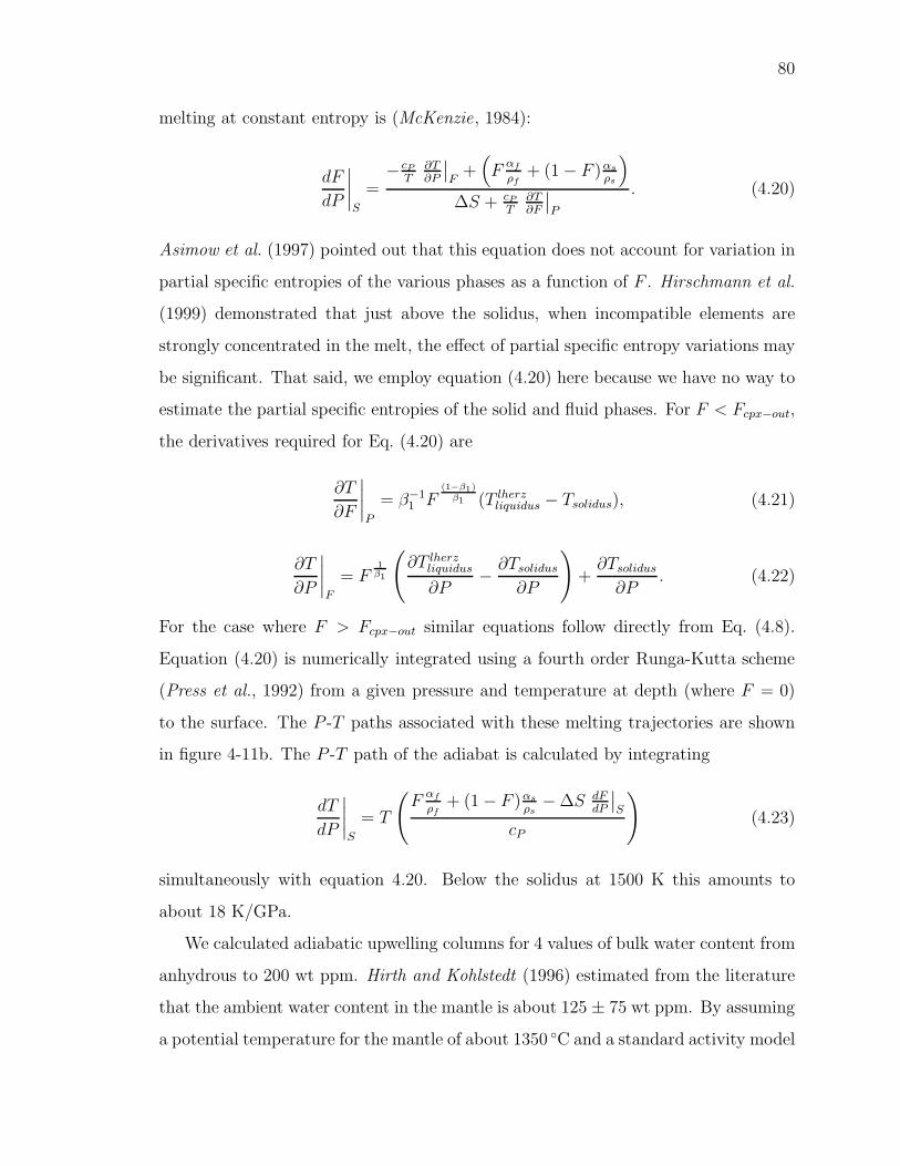
80
melting at constant entropy is (McKenzie, 1984):
dF
dP
∣
∣
∣
∣
S
=− cP
T∂T∂P
∣
∣
F+(
Fαf
ρf+ (1 − F )αs
ρs
)
∆S + cP
T∂T∂F
∣
∣
P
. (4.20)
Asimow et al. (1997) pointed out that this equation does not account for variation in
partial specific entropies of the various phases as a function of F . Hirschmann et al.
(1999) demonstrated that just above the solidus, when incompatible elements are
strongly concentrated in the melt, the effect of partial specific entropy variations may
be significant. That said, we employ equation (4.20) here because we have no way to
estimate the partial specific entropies of the solid and fluid phases. For F < Fcpx−out,
the derivatives required for Eq. (4.20) are
∂T
∂F
∣
∣
∣
∣
P
= β−11 F
(1−β1)β1 (T lherz
liquidus − Tsolidus), (4.21)
∂T
∂P
∣
∣
∣
∣
F
= F1
β1
(
∂T lherzliquidus
∂P−∂Tsolidus
∂P
)
+∂Tsolidus
∂P. (4.22)
For the case where F > Fcpx−out similar equations follow directly from Eq. (4.8).
Equation (4.20) is numerically integrated using a fourth order Runga-Kutta scheme
(Press et al., 1992) from a given pressure and temperature at depth (where F = 0)
to the surface. The P -T paths associated with these melting trajectories are shown
in figure 4-11b. The P -T path of the adiabat is calculated by integrating
dT
dP
∣
∣
∣
∣
S
= T
(
Fαf
ρf+ (1 − F )αs
ρs− ∆S dF
dP
∣
∣
S
cP
)
(4.23)
simultaneously with equation 4.20. Below the solidus at 1500 K this amounts to
about 18 K/GPa.
We calculated adiabatic upwelling columns for 4 values of bulk water content from
anhydrous to 200 wt ppm. Hirth and Kohlstedt (1996) estimated from the literature
that the ambient water content in the mantle is about 125 ± 75 wt ppm. By assuming
a potential temperature for the mantle of about 1350 C and a standard activity model

81
for water in silicate melts, they predicted that melting should begin under ridges at
about 115 km depth, well within the garnet stability field. Our calculations agree
quite well with these estimates, as shown in Figure 4-11.
Figures 4-11a and b show 12 separate calculations, four bulk water contents at
three different mantle potential temperatures. The results agree with the widely held
view that water extends the depth interval of melting significantly, putting a larger
portion of the total melt generation at higher pressures and increasing the average
pressure of melting (Asimow and Langmuir , 2003). In figure 4-11c we quantify this
effect by plotting the pressure interval over which the first one percent of melting
occurs.
4.6.2 Arc Melting
As a first step toward applying this melting parameterization to subduction zone
magma genesis simulations, we calculate a two dimensional melting field on an arc
thermal structure with a specified mantle flow field. We apply a constant bulk water
concentration evenly over a triangular region of the wedge. The thermal structure
is determined by solving a time dependent advection-diffusion equation of energy
conservation without melting (we use a Semi-Lagrangian Crank-Nicholson algorithm,
see Katz et al. (2003), in prep.). The thermal calculation is run to steady state and the
resulting temperature field is used as an input to the melting calculation. Enthalpy
is conserved at each grid point in this calculation according to the equation
cPTi = (cP + F∆S)Tf . (4.24)
Here, Ti is the temperature before melting and Tf the final temperature after melting.
Tf must be consistent with the final degree of melting, F , according to the melt
parameterization. Modal cpx is taken as 17 wt%. Results of an example calculation
are shown in figure 4-12. We explore this model further in Langmuir et al. (in prep)
to understand how subduction parameters such as convergence rate and slab dip will
affect the degree of melting in the wedge and compare it to Na variations observed

82
in arc lavas.
4.7 Summary
We have presented a new parameterization of anhydrous and hydrous melting of man-
tle peridotite that takes into account the pressure, temperature, water content and
modal cpx of a melting system to calculate the equilibrium degree of melting. Our
parameterization includes many of the important features of hydrous melting of peri-
dotite observed in experiments and predicted by theory. It remains mathematically
simple, efficient to compute and flexible to modification as experiments and theory
on peridotite melting evolve.
A comparison of isobars shows that all anhydrous parameterizations lie within the
experimental variance at moderate pressure. All succeed to a similar degree in fitting
the data. Furthermore, all of the parameterizations demonstrate concave upward
low-F tails under hydrous conditions. An important difference between the models
is their near-solidus behavior under anhydrous conditions.
The first preliminary test of the model, an adiabatic melting calculation, demon-
strates that its predictions agree quantitatively with observations and theory (Hirth
and Kohlstedt , 1996). An increasing pressure interval for the first 1% melting is consis-
tent with expectations and has important implications for trace element partitioning.
Application of the parameterization to a subduction zone thermal calculation gives
reasonable results and will be coupled with full fluid and solid flow and geochemical
transport in future work.
This parameterization is, of course, a simplification of the natural system that it
aims to represent. For example, mineral composition, especially enrichment in easily
fusible elements, plays an important role in determining the solidus and the shape of
the melting function (Pickering-Witter and Johnston, 2000; Schwab and Johnston,
2001). This compositional variability is not captured by our parameterization.
To account for greater variability in the system would require a more complicated
model. Given current uncertainties in experimental and theoretical constraints on

83
mantle melting, as well as the need to maintain computational efficiency, we feel that
this parameterization contains an appropriate level of detail. It strikes a balance
between efficiency and accuracy and delivers output that will be useful in tectonic
scale models of magma genesis in subduction zones.

84
(a) 0 10 20 30 40 50 600
100
200
300
400
500
600
700
800
900
Water in the melt, wt%
∆T, S
olid
us s
hift
in ° C
Gaetani & Grove, 98Hirose & Kawamoto, 95Grove AGU, 01Kawamoto & Holloway, 97Parameterization
(b)0 2 4 6 8
0
10
20
30
40
50
Pressure, GPa
Wat
er in
the
mel
t at s
atur
atio
n, w
t%ParameterizationDixon & Stolper: regular solution modelMysen & Wheeler: experiments
Figure 4-8: (a)The calibration of ∆T (XH2O) for the parameters K and γ from equa-tion 4.16. Data is derived from the experiments of Hirose and Kawamoto (1995),Kawamoto and Holloway (1997), Gaetani and Grove (1998), and Grove (2001). Re-sult is given in table 4.2. (b) The saturation water content in wt% of the melt asa function of pressure from equation 4.17. Points are from Dixon et al. (1995), whoreport a regular solution model for basalt up to 0.5 GPa based on their and otherexperiments, and Mysen and Wheeler (2000), who report the saturation water con-tent for three haploandesitic compositions (shown are results from the aluminum freecomposition that is 79% SiO2).

85
1200 1300 1400 1500 1600 1700 18000
0.05
0.1
0.15
0.2
0.25
0.3
0.35
0.4
0.45
0.5
Temperature, °C
Mel
t fra
ctio
n, F 1 GPa
3 GPa
New modelMcKenzie&BickleLangmuir92Iwamori95pMELTS
Figure 4-9: A comparison of the results of several parameterizations of dry meltingand pMELTS calculations at 1 (in blue) and 3 (in green) GPa. The parameterizationsare described by Langmuir et al. (1992), McKenzie and Bickle (1988) and Iwamoriet al. (1995). pMELTS is described by Ghiorso et al. (2002). A commonly usedparameterization by Kinzler and Grove (1992) is not considered because it requiresthe input of chemical information.

86
(a)800 1000 1200 1400 1600 1800
0
0.1
0.2
0.3
0.4
0.5
Temperature, °C
Mel
t fra
ctio
n, F
0.1 wt% bulk water
1 GPa 3 GPa
New modelDavies&BickleLangmuir
(b)800 1000 1200 1400 1600 1800
0
0.1
0.2
0.3
0.4
0.5
Temperature, °C
Mel
t fra
ctio
n, F
0.5 wt% bulk water
1 GPa 3 GPa
New modelDavies&BickleLangmuir
Figure 4-10: A comparison of parameterizations of mantle melting in the presenceof water at 1 and 3 GPa. Asimow and Langmuir (2003) use a hydrous extensionof the anhydrous parameterization described by Langmuir et al. (1992). Davies andBickle (1991) extends the McKenzie and Bickle (1988) parameterization to handlewet melting. (a) For bulk water content of 0.1 wt%. (b) For bulk water content of0.5 wt%.

87
(a)
0 0.05 0.1 0.15 0.2 0.25
0.5
1
1.5
2
2.5
3
3.5
4
4.5
5
5.5
6
Pre
ssur
e, G
Pa
Melt Fraction
θ=1450°C
θ=1350°C
θ=1250°C
0
60
120
180
Depth, km
(b)
1200 1300 1400 1500
0.5
1
1.5
2
2.5
3
3.5
4
4.5
5
5.5
6
Pre
ssur
e, G
Pa
Temperature, °C
Dry solidus
0
60
120
180
Depth, km
(c) 0 50 100 150 2000.2
0.25
0.3
0.35
0.4
0.45
0.5
0.55
0.6
0.65
0.7
Bulk water, wt ppm
∆P o
f firs
t 1%
mel
ting,
GP
a
θ=1450°C
θ=1350°C
θ=1250°C
Figure 4-11: Results of the numerical integration of equations 4.20 and 4.23 for amantle with bulk water ranging from 0 to 200 wt ppm and modal cpx of 10 wt%.Values of all melting model parameters are as given in table 4.2. Some of the curvesshow a kink due to cpx-out. (a) F (P ). (b) T (P ). (c) A quantification of the waterinduced low-F tails on adiabats. The pressure interval over which the first one percentof melting occurs is plotted as a function of bulk water in the system and potentialtemperature.

88
(a)0
500
1000
1500
Distance, km
Pre
ssur
e, G
Pa
Temperature after melting
0 50 100 150 200 250 300 350 400 450 500
0
1
2
3
4
5
6
7
8
9
(b)
1
2
3
4
5
6
7
8
9
Distance, km
Pre
ssur
e, G
Pa
Degree of melting
0 50 100 150 200 250 300 350 400 450 500
0
1
2
3
4
5
6
7
8
9
Figure 4-12: A representative example of a two dimensional static arc melting calcu-lation. Bulk water of 0.5 wt% is applied only over the corner of the wedge shown in(b). The potential temperature of the mantle is taken to be 1350 C. (a) Temper-ature of equilibration. (b) Equilibrium degree of melting in percent melt by mass.Maximum is 9.3%.

89
Chapter 5
Reactive hydrous melting andchannelized melt transport in arcs
Abstract
Magma genesis in subduction zones has long been recognized as an open system pro-cess with fluxes of heat, mantle rock, hydrous fluids and magma moving along differentpaths through the system. Fluids released from the subducting slab interact with themantle wedge and produce silicate melts that rise toward the lithosphere; some of thismelt is eventually erupted from arc volcanoes. To develop a quantitative understand-ing of this process requires models capable of calculating both solid and fluid flow,adiabatic and reactive hydrous melting and temperature evolution. As a step towardsuch a model, we have parameterized a pseudo-phase diagram of a simplified rock–water system that describes the composition of water-bearing fluids in equilibriumwith the silicate mantle. By extending a preexisting framework for reactive magmatransport, we can use this pseudo-phase diagram to calculate reactive melting andfreezing rates in a two dimensional model of a subduction zone. Our results showthat channelization of fluid flux in the thermal boundary layer above the slab is anexpected consequence of melting reactions in arcs. Furthermore, calculations suggestthat when channels interact with the lithospheric thermal boundary layer they co-alesce into bundles of channels that advect enough heat to modify the topographyof the boundary layer. We discuss some implications of channelized melt transportpredicted by the model and propose future work that would help to understand andquantify the results obtained here.
5.1 Introduction
Magma genesis in subduction zones has long been recognized as an open system
process, from early conceptual diagrams (Ringwood , 1974) to recent computational
models (e.g. Gerya and Yuen, 2003; Iwamori , 1998). The heat flux required for

90
sustained melting over geologic time is delivered by advection of hot mantle material
into the wedge (Kelemen et al., 2002; van Keken et al., 2002). Volatiles, considered
to be an essential component of subduction zone magma, are carried to depth by the
subducting slab and liberated from it beneath the wedge by metamorphic reactions
(Stern, 2002, and refs. therein). At least some of the magma which is produced leaves
the system through the crust, carrying with it heat and volatiles as well as trace and
major elements from a variety of sources at depth (Miller et al., 1994).
Distinct geochemical evidence exists for two modes of melt generation in the man-
tle wedge: (1) Hydrous melting of mantle peridotite due to a flux of volatiles and (2)
anhydrous melting of mantle peridotite due to adiabatic upwelling of mantle peri-
dotite (Sisson and Bronto, 1998; Kelley et al., 2004). Modern computational models
of variable viscosity momentum and energy conservation in the mantle wedge produce
flow and temperature fields consistent with simultaneous magma genesis in both of
these modes (see chapter 3).
Temperature and solid flow fields in the mantle wedge hence constitute the con-
text for melting. As such, they are of fundamental importance. However, to develop
a quantitative understanding of magma genesis in subduction zones requires models
that calculate melt transport as well as mass transfer reactions such as melting–
freezing and hydration–dehydration. Previous authors have described models of
porous fluid transport in subduction zones (Davies and Stevenson, 1992; Iwamori ,
1998). Recent work by Baker et al. (2004) incorporates full mantle thermodynamics,
as described by the MELTS algorithm (Ghiorso et al., 2002), into an open system
subduction model. These authors treat the hydrous fluid presumed to rise off the
slab as a passive phase which is transported by solid advection and buoyancy–driven
porous flow. By neglecting reactivity of the fluid and pressure forces arising from vis-
cous compaction of the mantle matrix (described below), these models miss what may
be a critical insight into the physics and chemistry of magma genesis in subduction
zones. In this chapter I present a model that can address these deficiencies.
Such models of reactive transport in subduction zones are based on past work on
mid-ocean ridges (Spiegelman et al., 2001; Spiegelman and Kelemen, 2003). Exper-

91
iments and observations of mid-ocean ridge derived basalts shows that these melts
are highly reactive as they rise toward the surface (Kelemen et al., 1995a; Liang and
Morgan, 2004), dissolving and reprecipitating mantle matrix phases. Aharonov et al.
(1995) showed that the formation of high flux porous channels between low permeabil-
ity compacted regions is a natural consequence of reactive porous flow up a solubility
gradient. These channels seem to correspond to the tabular refractory dunite bodies
surrounded by harzburgite observed in the Oman ophiolite (Kelemen et al., 1995a;
Braun and Kelemen, 2002).
Taken together, these calculations constitute a theoretical framework for modeling
open system reactive melt transport. Here we describe an extension of that framework
to the more complex case of magma genesis in subduction zones. We explicitly model
the corrosive reactivity of an aqueous fluid rising from the top of the cool slab to the
core of the hot mantle wedge and compute fluid transport using the full physics of
porous flow in a viscously compatible medium as derived by McKenzie (1984) and
outlined in chapter 1 of this thesis. As in the case of flow up a solubility gradient
beneath mid-ocean ridges, fluids rising off the subducting slab react and localize into
high flux channels. An example calculation is shown in 5-3. Channelized melts are
predicted to have higher water contents and travel toward the Moho with greater
speed. Furthermore, our calculations show that the heat transported by channelized
fluids is sufficient to locally modify the temperature field.
5.2 Reactive melting
5.2.1 Chemistry
Experimental studies have shown that metamorphic reactions at depth in the sub-
ducting slab exsolve a dilute aqueous fluid (e.g. Schmidt and Poli , 1998; Forneris and
Holloway , 2003; Manning , 2004). Subduction zone volcanics, on the other hand, are
usually derived from silicate liquids with a small fraction of dissolved water. Between
departure from the subducted slab and arrival at the volcano a vast change in silicate
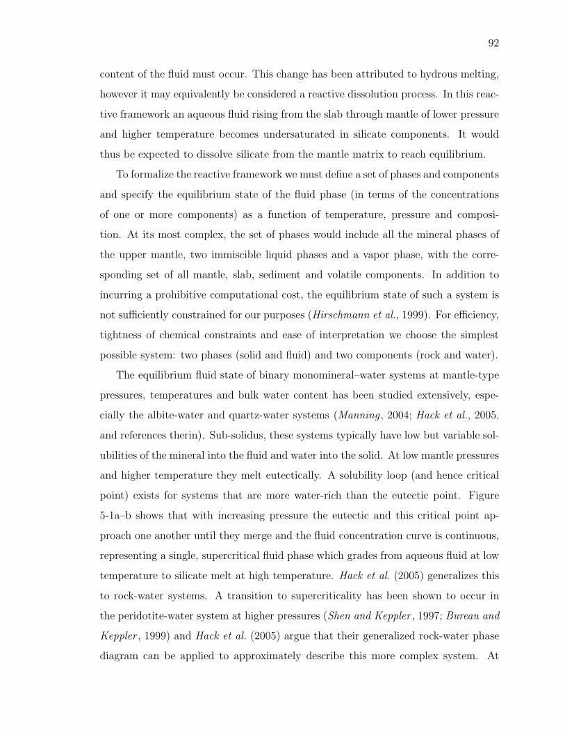
92
content of the fluid must occur. This change has been attributed to hydrous melting,
however it may equivalently be considered a reactive dissolution process. In this reac-
tive framework an aqueous fluid rising from the slab through mantle of lower pressure
and higher temperature becomes undersaturated in silicate components. It would
thus be expected to dissolve silicate from the mantle matrix to reach equilibrium.
To formalize the reactive framework we must define a set of phases and components
and specify the equilibrium state of the fluid phase (in terms of the concentrations
of one or more components) as a function of temperature, pressure and composi-
tion. At its most complex, the set of phases would include all the mineral phases of
the upper mantle, two immiscible liquid phases and a vapor phase, with the corre-
sponding set of all mantle, slab, sediment and volatile components. In addition to
incurring a prohibitive computational cost, the equilibrium state of such a system is
not sufficiently constrained for our purposes (Hirschmann et al., 1999). For efficiency,
tightness of chemical constraints and ease of interpretation we choose the simplest
possible system: two phases (solid and fluid) and two components (rock and water).
The equilibrium fluid state of binary monomineral–water systems at mantle-type
pressures, temperatures and bulk water content has been studied extensively, espe-
cially the albite-water and quartz-water systems (Manning , 2004; Hack et al., 2005,
and references therin). Sub-solidus, these systems typically have low but variable sol-
ubilities of the mineral into the fluid and water into the solid. At low mantle pressures
and higher temperature they melt eutectically. A solubility loop (and hence critical
point) exists for systems that are more water-rich than the eutectic point. Figure
5-1a–b shows that with increasing pressure the eutectic and this critical point ap-
proach one another until they merge and the fluid concentration curve is continuous,
representing a single, supercritical fluid phase which grades from aqueous fluid at low
temperature to silicate melt at high temperature. Hack et al. (2005) generalizes this
to rock-water systems. A transition to supercriticality has been shown to occur in
the peridotite-water system at higher pressures (Shen and Keppler , 1997; Bureau and
Keppler , 1999) and Hack et al. (2005) argue that their generalized rock-water phase
diagram can be applied to approximately describe this more complex system. At

93
pressures below the transition to supercriticality this argument breaks down. How-
ever, as we show in Figure 5-1a–c and discussed below, the error resulting from this
assumption is small.
A continuous solubility curve is convenient because it is consistent with past work
on reactive flow modeling and because it stabilizes numerical solvers. Although the
pressures relevant for subduction zone magma genesis are lower than those required
for supercriticality in the peridotite-water system, we assume that for low bulk water
contents a continuous solubility curve is a good approximation. This is supported by
the observation that water and other incompatible elements present in low concen-
tration cause a “low productivity tail” in the isobaric melting curve as a function of
temperature (Hirschmann et al., 1999). Furthermore, it is generally accepted that
there is no eutectic for peridotite melting. Figure 5-1c shows that there is only a small
difference in dissolved silica content as a function of temperature along a supercritical
curve and a eutectic melting curve.
To parameterize the sigmoidal curve described by Hack et al. (2005), we specify
the solubility of rock into the fluid as a function of temperature and pressure at fixed
bulk water content. A convenient form is:
f(T ′) =(
1 + αT ′β)
tanhT ′
λ(5.1)
where T ′ = 2T/Tdry liquidus − 1. This definition for T ′ is chosen to control the position
of the solidus in temperature by fixing it as one half the temperature of the liquidus,
in degrees centigrade. For T ′ > 0, α = α1(P ) and β = β1 while for T ′ < 0, α = α2
and β = β2. α1 is a linear function of pressure. The equilibrium concentration of
rock in the fluid is then
Cf(T′) =
f(T ′) + 1 + α2
2 + α1 + α2. (5.2)
The pressure dependence of solubility can be accounted for by giving Tdry liquidus a
quadratic dependence on pressure as in Katz et al. (2003). We then calibrate this
function by fitting it (by inspection) to the output of a parameterization of hydrous
melting (Katz et al., 2003). The large number of parameters in this formulation arise
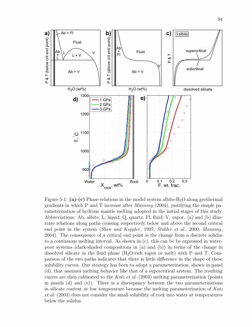
94
Fluid
Fluid
L + VAb+L
Ab+Fl
Ab + V Ab + V
H2O (wt%) H2O (wt%)
a) b) c)
P &
T
P &
T (
belo
w c
rit
end p
oin
t)
P &
T (
above c
rit en
d p
oin
t)
dissolved silicate
supercritical
subcritical
+albite
L V
V
Ab + Fl
e)
RockWater
900
1000
1100
1200
1300
Xrock
, wt%
T,
°C
1 GPa
2 GPa
3 GPa
0 0.1 0.2 0.3
F, wt. frac.
d)
Figure 5-1: (a)-(c) Phase relations in the model system albite-H2O along geothermalgradients in which P and T increase after Manning (2004), justifying the simple pa-rameterization of hydrous mantle melting adopted in the initial stages of this study.Abbreviations: Ab, albite; L, liquid; Q, quartz; Fl, fluid; V, vapor. (a) and (b) illus-trate relations along paths crossing respectively below and above the second criticalend point in the system (Shen and Keppler , 1997; Stalder et al., 2000; Manning ,2004). The consequence of a critical end point is the change from a discrete solidusto a continuous melting interval. As shown in (c), this can be be expressed in water-poor systems (dark-shaded compositions in (a) and (b)) in terms of the change indissolved silicate in the fluid phase (H2O-rich vapor or melt) with P and T. Com-parison of the two paths indicates that there is little difference in the shape of thesesolubility curves. Our strategy has been to adopt a parameterization, shown in panel(d), that assumes melting behavior like that of a supercritical system. The resultingcurves are then calibrated to the Katz et al. (2003) melting parameterization (pointsin panels (d) and (e)). There is a discrepancy between the two parameterizationsin silicate content at low temperature because the melting parameterization of Katzet al. (2003) does not consider the small solubility of rock into water at temperaturesbelow the solidus.

95
from designing an easily tuned curve that is specified in a symmetric manner around
the solidus. A more careful study could reduce the number of parameters. The shape
of the curve, however, and the eventual results obtained by using it in reactive melting
calculations, would be largely unchanged.
Results of this calibration are shown in Figure 5-1d–e. Although we calibrate
our parameterization of equilibrium solubility for a 2 wt% bulk water content sys-
tem, we find that the solubility parameterization is in agreement with the melting
parameterization for bulk water contents between 0.1 and 3 percent. The use of a
pseudo-phase diagram to prescribe melting properties of the rock–water system pro-
duces a result inconsistent with observations (e.g. Stolper and Newman, 1994) and
theoretical predictions (e.g. Katz et al., 2003), however. According to the pseudo-
phase diagram parameterization, a system at a fixed temperature will vary in melt
fraction with increasing bulk water to maintain constant water content of the melt.
In constrast, the generally held view is that at a fixed temperature, addition of bulk
water to the system will cause melt fraction to increase but less rapidly, such that
the water content of the melt actually increases with increasing melt fraction. If the
melting system indeed functions according to the latter scenario there may be conse-
quences for predicted water content of melts that are not captured by the simulations
described here.
With the solubility of rock in water expressed as a function of pressure and tem-
perature and given a vertical temperature profile, a vertical profile of porosity and
fluid composition can be calculated that is in a steady state, using the governing
equations in the limit of zero compaction length. In this state, if we consider the high
Damkohler number limit of the conservation of composition equation for the fluid
and assume that the solid matrix is static and that there is an instantaneous balance
between advection and reaction we find that the melting rate, Γ, scales as
Γ ∝φw
CR − Cf
∂Ceqf
∂P(5.3)
where φ is the volume fraction of melt, w is the vertical velocity of the melt, CR −Cf

96
is the difference between the concentration of rock in the reaction product and in
the fluid, and ∂Ceqf /∂P is the slope of the equilibrium solubility curve along the
arc geotherm. Figure 5-2 shows two temperature distributions and their resulting
equilibrium and melting rate curves. The temperatures are imposed as an initial
condition (and a reference state for the source term in equation (5.5)) but the melting
rate and the equilibrium concentration of rock in the fluid are determined by solving
the steady-state, zero compaction length approximation of the governing equations.
5.2.2 Physics
The physics of reactive open–system melt transport through a viscously deformable
porous medium has been described by other authors (e.g. Spiegelman et al., 2001).
The conservation of mass equations for individual components, which augment the
conservation equations in chapter 1, are presented by Spiegelman et al. (2001) and
will not be repeated here. To extend this system for a temperature–dependent fluid
equilibrium we require knowledge of temperature over the domain. Hence, in addition
to the equations described by Spiegelman et al. (2001), we enforce the conservation
of energy expressed as a temperature evolution equation. A conservation equation
for the energy of a two-phase continuum with mass transfer representing magma-
genesis in the mantle was derived by McKenzie (1984) and is given in expanded form
in equation (1.7). We neglect changes in temperature due to (de)compression and
differences in specific heat and thermal diffusivity between the solid and fluid phases.
With these simplifications equation (1.7) becomes
∂T
∂t+ vT · ∇T =
−T∆S
ρcPΓ + κ∇2T + S(φ, T,x), (5.4)
where vT =ρf φv+ρs(1−φ)V
ρis the velocity at which heat is advected and ρ = ρfφ +
(1−φ)ρs is the porosity-weighted density. This equation states that the temperature
at a point fixed in the two-dimensional domain is controlled by advection, latent heat
transfer, diffusion and a source term. Except for compaction and expansion, the solid
is static in the simplified computations described here and thus advection of heat

97
900 1000 1100 1200
2
2.5
3
Pre
ssur
e, G
Pa
Temperature, °C
water rock
CRockf,eq
0 2 4 6 8
Melting rate, Γ
Figure 5-2: Two initial condition of vertical distribution of temperature and theresulting equilibrium content of rock in the fluid and dimensionless melting rate.The green line shows the initial condition for the calculation shown in Figure 5-3and the red line shows the initial condition for Figure 5-4. (a) Imposed verticaltemperature profile. The green line is a crude representation of the temperature fieldimmediately above the slab: temperatures increase upward. The red line representsthe temperature field between the slab and the bottom of the lithosphere. Both ofthese are simple approximations to a more realistic geotherm shown in Figure 5-6. (b)Equilibrium concentration of rock in the fluid given the temperature-pressure curvein panel (a). (c) Dimensionless melting rate given the temperature-pressure curve inpanel (a). Note that precipitation is occurring at the bottom of the lithosphere in thesimulation initiated with the red temperature profile. The curves in panels (b) and(c) are calculated by solving the steady-state, zero compaction length approximationof the governing equations.

98
is mainly by the fluid. Without transport of heat into the wedge by solid mantle
flow, however, melting and melt transport would rapidly cool the wedge. We roughly
approximate this advection of heat into the plane of the simulation with the source
term S in equation (5.4). We assume that the solid mantle advected into the domain
has the temperature structure of the initial T -field of the simulation and that its
motion does not displace the pore fluids. With these assumptions the source term is
S(φ, T,x) = τ(1 − φ) [T (x, t = 0) − T (x, t)] (5.5)
where τ has dimension of inverse time and is a number between zero and one parame-
terizing the fraction of the solid replaced with new solid advected in from outside the
domain, carrying heat with it. The value of τ is typically set to be 0.03 kyrs−1. The
value of τ is set to keep the simulations from changing its temperature field too much
from the intial temperature field. It should be noted, however, that this parameter is
poorly constrained and the effect of variations has not been carefully explored.
The boundary conditions specified on the top boundary are very important for
the behavior of the simulation. The vertical gradient in the compaction potential is
set to zero across this boundary, although the horizontal gradient is not specified,
allowing for compaction at and near the boundary. The gradient in concentration
of the solid is also set to zero. This condition has little effect. The equilibrium
fluid concentration is calculated as within the domain. The fluid concentration is
also calculated as within the domain, however that fluid velocity on the boundary is
calculated differently from inside the domain. The fluid velocity on the boundary is
computed assuming zero dynamic pressure gradient—that is, the pressure gradient
there is due to fluid buoyancy only. Finally, and most importantly for what is to
follow, the temperature conditon on the boundary is very loose: it specifies that there
is no diffusion of temperature on the boundary by setting d2T/dz = 0. It is only the
effect of the source term, which acts as a “restoring force” on the temperature at every
point in the domain, which forces the simulation to remain close to a given value of
temperature at the boundary. This is, in effect, a mixed boundary condition. It

99
allows the advection of heat by the fluid to modify the temperature on the boundary.
Another important aspect of these calculations is how we treat the bulk viscosity.
We adopt a form for the viscosity governing compaction proposed by Sleep (1988)
and used by Spiegelman et al. (2001),
(ζ + 4η/3) =(φc/φ)m + 4/3
φmc + 4/3
. (5.6)
This equation states that the compaction viscosity (ζ + 4η/3) is nearly constant for
porosities greater than the “compaction viscosity” φc, but becomes infinite for φ φc.
We solve the magma dynamics equations plus conservation of energy and com-
position using the Portable Extensible Toolkit for Scientific computation (PETSc,
Balay et al., 1997, 2001, 2002) on a domain oriented parallel to the strike of the arc
as shown in Figure 5-3a. The base of the domain sits just above the surface of the
subducting slab and thus receives a flux of slab-derived fluids from below. The top
of the domain is positioned either at the core of the wedge (green lines in Figure 5-2
and results in Figure 5-3) or above it in the the upper thermal boundary layer of the
wedge (red lines in Figure 5-2 and results in Figure 5-4). Orientation of the domain
in this manner is convenient because it permits us to employ a simple, rectangular
grid and a wrap-around boundary condition on the side boundaries.
5.3 Results
Fluid channelization is an expected consequence of the Reaction Infiltration Insta-
bility (Chadam et al., 1986; Daccord and Lenormand , 1987; Aharonov et al., 1995),
which is active when a reactive fluid percolates through a soluble matrix from a zone
of lower solubility to a zone of higher solubility. Regions with higher melt flux un-
dergo more dissolution (as is evident in equation (5.3)) and thus a higher porosity,
permeability and melt flux. Small perturbations grow and lead to a channelized
porosity/permeability structure (Aharonov et al., 1997; Spiegelman et al., 2001).

100
5.3.1 Flow from the slab surface to the core of the mantle
wedge
Models of reactive flow from the slab to the core of the wedge have results that are
easy to interpret in terms of past work on reactive magmatic flow (Spiegelman et al.,
2001). The flux of magma in these calculations rapidly localizes into high porosity
channels, shown at a late simulation time in Figure 5-3b. High rates of reaction are
observed in calculations where fluid crosses the “wet solidus” of the rock phase. This
is the temperature at which the equilibrium concentration of the fluid shifts sharply
from water-rich to rock-rich, shown in Figure 5-1d. The corresponding increase of
the reaction rate Γ with height is shown in Figure 5-2c. Fang and Spiegelman (2004)
suggested that the rate of channelization in compactible systems is related to the
change in solubility over a compaction length. Hence it is not surprising that channels
in Figure 5-3b nucleate at a height in the domain where the reaction rate is at its
peak.
In the calculation of hydrous reactive flow in Figure 5-3b, porosity in the channels
is around 10% (although they grow larger than this with time) while inter-channel
regions compact down to less than 1% porosity, although the latter depends on the
details of the assumed bulk viscosity. Figure 5-3c shows that channels are marked by
fast vertical velocities. Fluid in channels in these calculations moves about 10 times
faster than fluids in diffuse porous flow calculations. This rapid ascent rate means that
channel fluids remain further from equilibrium than inter-channel fluids. Contours in
Figure 5-3b show the mass fraction of water content in the fluid and demonstrate that
fluid rising rapidly through the channels is enriched in water relative to fluid outside
the channels. This is not due solely to the disequilibrium between the rising fluid and
the mantle matrix, however. Contours in Figure 5-3c show that the localized flux of
fluids through the channels modifies the temperature field. Fluids flowing from colder
to hotter temperatures cool the surrounding matrix rock. This cooling is enhanced by
the removal of heat from the matrix to balance the latent heat of dissolution reactions,
which are concentrated in the channels. In the calculations these effects are manifest

101
Pre
ssu
re,
GP
a
950
1000
1025
1050
1070
1090
1110
1130
1150
Temperature, °C
3
2.5
2
0
2
4
6
8
10
12
0.75
0.7
0.65
0.6
0.55
0.5
0.45
0.4
0.35
0.3
0.25
0.2
0.15
0.1
Conc. WATER in FLUID3
2.5
2
0
2
4
6
8
10
12P
ressure
, G
Pa
fluid
velocity, m/y
r
Po
rosity, vol%
Computationaldomain
slab
wedge
(c)
(b)
(a)
(b)
Figure 5-3: Results from one time-step of a simulation of hydrous reactive flowthrough the inverted thermal boundary layer in the mantle wedge above the sub-ducting slab. (a) Schematic diagram illustrating position and orientation of thecomputational domain with respect to the trench and subducting slab. (b) Snapshotof porosity (colors) and weight fraction of water in the fluid (contours). (c) Verticalfluid velocity in cm/year (color) and temperature in degrees centigrade (contours).

102
in channels that are colder than the surrounding rock by about 20 degrees centigrade
above the slab in the core of the wedge. The effect of lower temperatures in channels
is to raise the equilibrium solubility of water, suppressing dissolution and making the
channel fluids more water-rich. As we shall see below, the opposite occurs as fluids
percolate from the wedge core to the colder lithosphere above.
The shape of channels is generally consistent with previous calculations by Spiegel-
man et al. (2001), however in the calculations described above, there seems to be
comparatively less upward coalescence of channels. This may be due to the fact that
calculations by Spiegelman et al. (2001) used a linear solubility curve with a constant
slope and an approximately constant compositional difference between the equilib-
rium fluid composition and the composition of fluid generated by dissolution, yielding
a channelization rate that is approximately constant with height in the box. Here, a
strongly non-linear solubility curve is used (Figure 5-1d), which yields a reaction rate
with a peak at the height where temperatures cross the solidus. Above this height in
the core of the wedge, steady-state fluid solubility is roughly constant with height and
reaction rates are lower. Channels that nucleated below in the reactive zone “coast”
through this unreactive zone, neither decaying nor coalescing. As we shall see below,
however, the situation changes when we consider the case of fluid flow from the cold
slab through the hot wedge and into the cold lithosphere.
5.3.2 Flow from the slab surface to the lithosphere overlying
the wedge
Magma erupted from arc volcanoes must traverse not just the hot wedge but also
the cold lithosphere. The base of the lithosphere is clearly visible in Figure 3-3
where viscosity changes by several orders of magnitude over a small distance. The
temperature at which this transition occurs is much higher than the temperature at
which peridotite becomes brittle. Thus, at least over a portion of the thickness of the
lithosphere, magma may travel via porous flow, as in the asthenospheric mantle. One
caveat to this logic is that if fluid pressures are high enough, they can cause the rock

103
to hydrofracture, even if it is hot. Lower temperatures in the lithosphere would be
expected to cause freezing (or equivalently, precipitation) of components of the rising
magma, enriching it in water. Volcanoes erupt lava, however; evidently magma must
traverse the mantle lithosphere to arrive at the brittle crust in some manner.
Simulations that impose an initial temperature field that increases with height
and then decreases show interesting and unexpected results. A time series of porosity
and temperature fields from a simulation is shown in Figure 5-4. In this simulation
an initial temperature profile given by the red curve in Figure 5-2a was prescribed.
The curve is not a profile derived from a thermal structure simulation (as in Figure
5-6) but the two share an important characteristic, namely that they are cold at the
depth of the slab-wedge interface, increase in temperature with height to a maximum
and then decrease back to colder temperatures below the surface.
Figure 5-4 shows a simulation that starts with a horizontally uniform porosity
field. With time, high porosity channels emerge. These channels coalesce into bundles
of channels. The coalescence point begins near the base of the cold lithosphere and
propagates downward. The result is a wide channel that carries a very high flux of melt
derived from ∼5 smaller channels that feed it. Contours in Figure 5-4 demonstrate
how the temperature field is affected by fluid flow and melting in the channel bundle:
below the core of the wedge the channel is cooler than its surroundings, above it is
warmer. The fluid advects enough heat to create a high temperature pathway through
the lithosphere. It traverses this pathway precipitating less rock than it would have if
it crossed the same height interval without a hot pathway. To understand this result
it is important to recall that the local temperature within the domain is controlled
by the balance of diffusion, (fluid) advection and a source term that represents heat
flow in the 3rd dimension. In the lithosphere where fluid advection acts to add heat
and increase the temperature, the source term acts to decrease the temperature. To
maintain a hot pathway through the lithosphere the flux of magma must transport
enough heat to balance losses. This is discussed further below.
Another noteworthy feature of the results, shown in Figure 5-5, is that the channel
bundles are capped, near the base of the upper thermal boundary layer, with a pod-

104
950
1000 1000 1000
1000
1050 1050 1050
1050
1100
1100
1150
1150
1180
11801180
3
2.5
2
0
5
10
15
20
950
1000
1050
1050
1100
1100
1150
1150
3
2.5
2
0
5
10
15
20
950
1000
1050 1050
1050
1100
1100
1150
1150
1180 1180
1180
1180
3
2.5
2
0
5
10
15
20
950
1000
1050
1050
1100
1100
1150
1150
1180
1180
3
2.5
2
0
5
10
15
20
t = 37.6
Pre
ssu
reP
ress
ure
t = 15.0 t = 22.5
t = 30.1
Figure 5-4: Porosity (color) and temperature (contours) at four non-dimensional timesin a hydrous reactive melting simulation. Temperature increases above the bottom ofthe domain into the wedge core and then, unlike in Figure 5-3, decreases with heighttoward the surface. Channels form and immediately begin to coalesce into bundlesthat tighten with time. These channel bundles carry a large flux of melt and are ableto significantly perturb the temperature field. Freezing melt near the top boundarylowers the permeability and confines outflow to narrow, high porosity gaps. Belowthese gaps, melt pools in high porosity zones. We are exploring hypotheses for themechanism of coalescence.

105
Pre
ssu
re,
GP
aP
ressu
re,
GP
a
Po
rosity
, Vo
l%V
ertic
al v
elo
city
, m/y
r
0.9
0.8
0.6
0.4 0.3
0.1
0.1
0.10.1 0.1 0.10.15
0.150.15
0.10.1
0.15
Conc. WATER in FLUID3
2.5
2
5
10
15
20
950
1000
1050
1100
1150
1180
1150
110010501000
Temperature, °C
2.5
2
2
4
6
8
10
12
14
3
(a)
(b)
Figure 5-5: Results from the same calculation as in Figure 5-4 comparing porosity,fluid composition, vertical fluid velocity and temperature fields. (a) Porosity field(color) with overlayed contours of water concentration in the fluid. Rapid flow throughthe channel bundles leads to high water concentrations in the bottom half of thedomain and that can persist through to the top of the domain. (b) Vertical fluidvelocity (color) with overlayed contours of temperature. Fluid velocities are calculatedassuming a velocity scale w0 of 1 m/yr after Spiegelman et al. (2001). This is aconservative estimate and may be low by 2 orders of magnitude. (Since time in thiscalculation is scaled by δ/w0, all rates scale with this ratio as well. So the input flux,the melting rate and the melt velocity all vary together with changes in w0.) Notethe stagnation of melt in the high porosity “pods” at the base of the cold thermalboundary layer.

106
shaped zone of high porosity where magma stagnates before moving rapidly through
the top of the domain. This may be a feature observable in seismic images of the
sub-arc lithosphere and mantle.
5.4 Discussion
The calculations described in this chapter indicate that flux channelization in sub-
duction zones is an expected consequence of the gradient in the solubility of rock
into the aqueous fluids that are released from the subducting slab. Fang and Spiegel-
man (2004) show that for reactive melting beneath mid-ocean ridges, channelization
is expected only if the ratio of melt upwelling velocity to solid upwelling velocity is
high and that the solubility gradient is sufficiently large (i.e. the solid viscosity is
sufficiently high). Rapidly upwelling fluids traverse the solubility gradient driving
reaction faster, yielding larger reaction rates relative to the adiabatic melting rate.
In subduction zones, upwelling of solid mantle may occur but its geometry is such
that flow is not directly upward, but sub-parallel to the slab, and hence not likely
to be as fast as melt upwelling rates. Furthermore, the solubility gradient of rock is
very steep as fluids cross the sharp temperature gradient above the slab (see Figure
5-6). Here the amount of dissolution per compaction length rise is much larger than
expected beneath ridges and hence the growth rate of the channelization instability is
very high. If the solubility model presented here is roughly correct, high permeability
channels are likely to be present in subduction zones. To further test this hypothesis,
however, many more calculations are needed.
Assuming that this model of fluid flux channelization in arcs is correct, it is in-
teresting to consider the predicted consequences for lava chemistry. The observation
of Radium disequilibria in young arc lavas by Turner et al. (2001), for example, and
the positive correlation of Radium disequilibria with Barium–Thorium ratios suggest
rapid transit of fluids from the slab to volcanoes in subduction zones (Turner , 2002).
The transport of fluids through high permeability channels could provide a pathway
for bringing radioactive nuclides from the subducting slab to volcanoes about an or-
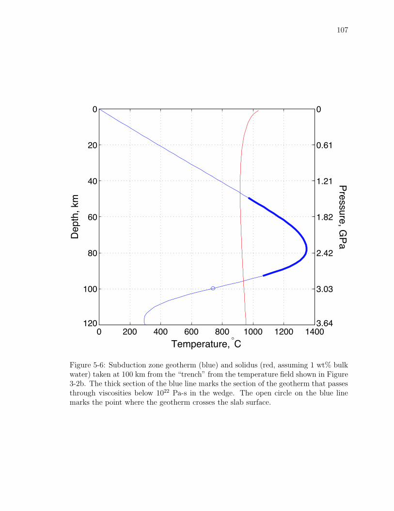
107
0 200 400 600 800 1000 1200 1400
0
20
40
60
80
100
120
Temperature, °C
De
pth
, km
0
0.61
1.21
1.82
2.42
3.03
3.64
Pressu
re, GP
a
Figure 5-6: Subduction zone geotherm (blue) and solidus (red, assuming 1 wt% bulkwater) taken at 100 km from the “trench” from the temperature field shown in Figure3-2b. The thick section of the blue line marks the section of the geotherm that passesthrough viscosities below 1022 Pa-s in the wedge. The open circle on the blue linemarks the point where the geotherm crosses the slab surface.

108
der of magnitude more rapidly than by diffuse flow. Assuming w0 = 1 m/yr, channel
velocities could be about 10 m/yr and 100 km of mantle could be traversed in 104
years (about 6 half-lives of Radium-226). If w0 is larger by an order of magnitude
then this time would be reduced to 1000 years. 103-104 years is within the range of
transit times preferred by Turner (2002).
Results shown in Figure 5-3 suggest that unlike diffuse porous flow, channelized
flow can modify the temperature structure of the two-phase medium. This has also
been observed in experiments by Solomon and Hartley (1998) on convection in a
mushy layer. In these experiments the Reactive Infiltration Instability produces open
chimneys that transport undersaturated melts at a different temperature than the
ambient surrounding permeable mush. The modification of local temperatures by
fluid flow has implications for equilibrium fluid composition as well as for arc heat
flow. Most significantly, models (e.g. Figure 5-4) predict that fluid flow can modify
the thermal structure at the base of the lithosphere, leading to focusing of flow,
melt pooling and high-temperature shallow equilibration. One can speculate that the
focusing that causes channels to coalesce into bundles is caused by an instability in the
interaction with a cold thermal boundary layer. This is illustrated schematically in
Figure 5-7. Channel-induced fluctuations in the thermal boundary layer topography
could reinforce magmatic focusing. This would occur according to a mechanism
proposed by Sparks and Parmentier (1991) whereby melt moves laterally along a cold,
sloping thermal boundary because colder temperatures directly above cause crystal
precipitation and decreased permeability. A feedback could result if melt focusing
modifies the local slope of the base of the lithosphere, leading to more focusing. If
such a focusing mechanism is active, the depth at which melts last equilibrate with
the mantle may be buffered by the extent to which advective heat transport can
preserve the ductile flow regime to shallow depths. Testing these ideas will require
the use of simplified computational models coupled with physical experiments.
Another interesting speculation that can be made about channel bundles and their
penetration into the lithosphere is that this process selects the along-arc spacing
of volcanoes. If coalescence of channels into bundles occurs by a thermal erosion

109
Cold and/or low porosity
Hot and/or high porosity
(d)(c)
(a) (b)
Figure 5-7: A schematic illustration of the proposed magmatic focusing instability.The blue regions represent cold, compact mantle. The pink areas represent hot,porous mantle. Red arrows represent highly porous channels. Channels impingeon the thermal boundary layer and perturb its topography. Melt follows upwardalong the sloping boundary by the mechanism proposed by Sparks and Parmentier(1991). This focusing produces more efficient thermal erosion of the boundary layerand coalescence of channels. As localized thermal erosion advances upward, regionsbetween the channel bundles compact and become almost impermeable, pushing thecoalescence point downward and forcing horizontal melt transport into the high-fluxchannel bundles.

110
process then the separation of these bundles may be controlled by thermal properties
of the magma/mantle system. For example, the diffusivity and heat capacity of
the lithosphere and the latent heat of freezing could all contribute to determining
the total flux of magma that must be focused in order to deliver enough heat to
penetrate the lithosphere. Then the spacing of volcanoes would reflect this required
flux. Uncertainties in the parameters that go into determining the compaction length,
especially the reference mantle viscosity and permeability, however, leads to variation
in the the predicted spacing of bundles by 2-3 orders of magnitude. Before simulations
of the complexity described here can be confidently interpreted, simpler models must
be used to test the validity of the focusing hypothesis.
5.5 Future work
Much work is required to better understand and quantify the results described here.
It can be divided into three general projects, however, that may each be undertaken
separately. The first two involve stripping complexity from the current model to
investigate the basic controls on channelization and channel coalescence. The third
project involves adding complexity to the model in order to generate testable geo-
chemical predictions.
We have shown that under reasonable assumptions regarding the compositional
equilibrium between a hydrous fluid and mantle, reactive flow calculations produce
channelized melt flux. The sensitivity of the result to these assumptions, both in
terms of the existence and characteristics of the channels, has not been investigated.
It would thus be useful to perform an exploration of parameter space associated
with the solubility gradient and equilibrium parameterization: the steepness and
profile of the temperature gradient itself, as well as the sharpness of the solidus
transition in the pseudo-phase diagram in Figure 5-1d. These calculations would be
done on a domain that extends from the slab to the wedge core, as in Figure 5-3.
Furthermore, simplifications to the physics and parameterized chemistry could be
made to eliminate parameters from the problem and isolate the fundamental controls
111
on the channelization instability in this system.
The coalescence of channels into channel bundles as shown in Figure 5-4 is an in-
triguing result of our calculations. Although this behavior was observed in a number
of model runs with cold lithospheric thermal boundary layers above the melting re-
gion, we can only hypothesize about the mechanism and relevant controls. Many more
simulations and analysis are needed to explore how the initial temperature structure,
temperature source term and thermodynamic parameters affect the predicted channel
structures. This should be done using the current model as well as a reduced model.
The domain of the reduced model would extend from the wedge core below through
the cold thermal boundary layer above. Equilibrium fluid inflow would be prescribed
at the base of the domain as either channelized flux or uniform flux. The reduced
model would incorporate a simplified parameterization of equilibrium fluid composi-
tion with a more gentle solidus transition to improve numerical convergence. This
model would permit an exploration of the physics of channel coalescence and melt
focusing through the lithosphere by isolating parameters that may be important such
as channel existence, spacing and flux, structure of the initial temperature profile and
the strength of the temperature source term.
Future calculations intended to explore melt–lithosphere interaction should be
accompanied by physical analog experiments like those carried out by Kelemen et al.
(1995b) that recreate the situation of precipitating reactive porous flow through a
cold thermal boundary layer. Experiments would provide a means for investigating
the focusing hypothesis described in Figure 5-7 without the assumptions that are
associated with a computational simulation of relatively high complexity.
A model capable of making predictions of geochemistry (such as an estimate of
Radium disequilibrium, discussed above) would be a useful tool for testing hypotheses
on the dynamics of subduction zones. It will necessarily be more complex than the
model described in this chapter. Simpler models are still essential for developing an
understanding of the basic behavior of the hydrous reactive system. The first step in
building a geochemical transport model is combining reactive flow calculations with
arc solid flow and thermal structure calculations from chapter 3 in a 2D domain ori-

112
ented perpendicular to the trench. This model would also need a parameterization
for fluid release from the subducting slab as well as a parameterization to calculate
adiabatic melting. With these components it would provide a self-consistent frame-
work for tracing the flow of energy and chemistry, including radiogenic isotopes, from
the slab to the base of the crust. There are many technical challenges that must be
overcome to build such a model, however, and therefore this project is a significant
undertaking.
5.6 Conclusion
The calculations presented here are a preliminary investigation into the consequences
of reactive flow in a subduction zone setting. Results show that channelization of
fluid flux is a physically plausible scenario in subduction zones and that channelized
flux is different in significant ways from diffuse porous flow. Some of these differences
may have observable consequences, such as rates of fluid transport from the slab to
the arc.
We have developed a new approach to modeling hydrous melting in arcs, one that
is based on experimental investigations of rock–water equilibrium and is well suited
to open-system reactive flow calculations. The parameterization of water content in
the fluid is formally consistent with previous work on reactive modeling of magma
transport (Spiegelman et al., 2001). However, it prescribes an equilibrium state that
is a function of both pressure and temperature, where previous work used a pressure-
dependent equilibrium. To supply temperature values to the parameterization we
solve the conservation of energy equation for the two-phase medium. This allows us
to explore thermal effects of reactive flow that had not previously been modeled. We
show that a channelized flux of fluids can modify the temperature field and hence the
equilibrium transport of solutes. We also show how advected heat delivered to the
base of the lithosphere can change the topography of this thermal boundary layer,
possibly resulting in magmatic focusing.
The results obtained here are qualitative. They show that by making a large

113
number of reasonable assumptions about the physics, chemistry and thermodynamics
of the magma/mantle system in subduction zones, a predicted instability leads to
channelization of fluid flux. The details of this process, including the spacing of
channels and their porosity, width and flux, are not quantitatively predicted by these
calculations. Numerical and analytical investigations conducted for this thesis as
well as elsewhere (Aharonov et al., 1995, 1997; Spiegelman et al., 2001; Fang and
Spiegelman, 2004) all suggest that the instability is robust: it occurs under a wide
range of parameters and mechanical assumptions. While much work remains to be
done to understand the characteristics and implications of channelized melt flow in
subduction zones, work presented here has demonstrated its physical plausibility for
the first time.

114
Chapter 6
Discussion
6.1 Summary
Much work is needed before models that are capable of addressing the questions raised
about subduction in the Introduction can be developed and interpreted. The chapters
of this thesis describe my research on general magma dynamics and subduction-related
dynamics that will be useful in reaching that long-term goal. Chapter 2 shows that
mechanical interactions between magma and mantle rock can lead to localization of
porosity and shear. The orientation of these localizations, if present in the Earth,
would affect the permeability structure of the mantle and have important implica-
tions for seismic anisotropy (Holtzman et al., 2003b). This orientation is shown to
be governed by the balance between porosity and strain rate-weakening mechanisms
of the two phase aggregate. The localization places significant demands on the com-
putational method and grid resolution of models. Preparations must be made to
handle these challenges if their presence is expected in large-scale magma dynamics
simulations.
Chapter 3 reports work on a single phase model of creeping mantle flow through
a subduction zone and the resulting temperature field. The results are similar to
those obtained by other investigators (van Keken, 2003b) and show the importance of
employing (at least) temperature-dependent viscosity. The role of stress and pressure-
dependence of viscosity in determining the flow field and thermal structure of arcs
(in steady-state), seems to be minor. The flow of fluids in a simple, constant porosity

115
model after Spiegelman and McKenzie (1987), however, is shown to be sensitive to
the inclusion of stress-dependence of viscosity, however. Stress-dependence was shown
in chapter 2 to have an important effect of melt flow and organization. In general,
variable viscosity models of arc thermal structure are consistent with the presence
of three modes of melting in subduction zones: adiabatic, reactive hydrous and slab
melting. Such models can serve only as the context for melting, however, because
they do not explicitly track fluids and interphase reactions.
A framework for reactive porous flow of fluids through the mantle exists (Spiegel-
man et al., 2001) but a simple, computationally efficient parameterization of hydrous
mantle melting that is accurate relative to current theoretical and experimental knowl-
edge was lacking. Chapter 4 addresses this gap and provides a means for rapidly
calculating equilibrium melt fractions and compositions in a simplified system of rock
(composed of olivine and pyroxene) and water. This work is useful not only for mod-
els of subduction, however, but as a general tool for geodynamic models of mantle
melting (see Appendix A, for example).
The melting parameterization presented in chapter 4 enabled the development of
the first model of reactive hydrous flow and melting in arcs described in chapter 5. It
is used to calibrate the rock–water pseudo-phase diagram critical for the adaptation
of previous work on reactive flow. Chapter 5 shows that the reactive flow of hydrous
fluids rising off the subducting slab into the mantle wedge may lead to channelization
of fluid/magma flux with consequences for predictions of the temperature field, rates
of fluid transport and fluid compositions in subduction zones. Furthermore, reactive
interactions with the lithosphere may lead to channel coalescence and could be related
to the along-arc spacing of arc volcanoes. The conclusions and speculations in this
chapter are exciting but need much more work to be understood and quantified.
The model described in this chapter may serve as a basis for the development of more
comprehensive models of subduction zone magma dynamics. Like the work in chapter
2 on mechanical localization, these calculations require high resolution computational
grids and advanced solvers. Further progress will require a reconsideration of the
numerical methods used here.

116
6.2 Open questions
Many interesting questions about the dynamics of volcanic source regions remain
unanswered. Several were listed in the introduction of this thesis. While this thesis
has attempted to address questions about magma dynamics in the mantle beneath
arcs, it has raised new questions about volcanic systems in subduction zones and
other tectonic settings. What follows is a review of some of the questions about the
dynamics of volcanic source regions that interest me.
6.2.1 Buoyancy effects
Buck and Su (1989) suggested that melting could cause active, focused upwelling at
mid-ocean ridges by lowering the density and viscosity of the solid–fluid aggregate
beneath the ridge. This would clearly be very important as a mechanism of melt
production at ridges as well as arcs and hot spots. Its plausibility, however, depends
quantitatively on the porosity–permeability relationship. If melt were easily drained
from the pores of the solid then melt would separate from the mantle under gravity
and would not drive upwelling of solid mantle. On the other hand, if the permeability
of the mantle were zero independent of porosity then melting would produce horizon-
tal buoyancy gradients of the two-phase aggregate and hence solid convection. The
permeability of the mantle lies somewhere between these extremes and hence to test
the hypothesis of Buck and Su (1989) requires a computational model with melting,
Darcy flow of magma and buoyancy-driven flow of the solid mantle. Such a study is
likely to be complicated by the presence of magmatic solitary waves, however.
Even if porosity-driven buoyancy is not important for upwelling and melting
of the mantle, active convection may be occurring in subduction zones. Kelemen
et al. (2002) showed that for a temperature-dependent viscosity and sufficiently large
Rayleigh number, cold lithospheric downwellings can perturb steady-state corner flow
and give it a time-dependent component. Calculations by Gerya and Yuen (2003)
suggest that cold plumes of chemically buoyant material could rise off the subducting
slab into the mantle wedge. While provocative, this latter hypothesis seems to rely on

117
low prescribed viscosities of hydrated mantle, slab and sediments. Furthermore, these
calculations do not account for the separation of fluids from solids and hence assume
that all fluid buoyancy is available for driving upwelling of the solid. A computa-
tional study that incorporates these effects and also allows for separation of fluid and
solid through porous flow would enhance our understanding of the role of buoyancy
in magma genesis in subduction zones.
6.2.2 Rheological effects
Chapter 2 of this thesis (as well as experiments and theory on melt localization going
back to Stevenson (1989)) demonstrated that the predicted behavior of a deforming
two-phase aggregate is drastically different depending on whether the aggregate is
modeled as porosity-weakening. To date, however, the effects of porosity weakening
of viscosity have only been explored in laboratory experiments and models of those
experiments. The important question of how porosity-weakening viscosity modifies
the predicted mantle and magmatic flow fields beneath an island arc, mid-ocean
ridge or hot-spot has not been addressed. Are strain rates in the partially molten
regions of the mantle large enough to produce porosity banding like that seen in
experiments? If so, where? What is the orientation of the emergent bands and how
do they interact with gravitationally driven magmatic flow? If strain rates are too
slow then the mechanical porosity band instability may not produce localization,
however high porosity channels resulting from a reactive dissolution instability would
presumably localize shear just as effectively, if they are suitably oriented.
6.2.3 Experimental constraints
Whether or not the mechanical instability discussed in chapter 2 is active in the
mantle, experiments by Holtzman et al. (2003a) provide a rare opportunity to directly
test the continuum theory of magma migration because they produce internal patterns
that can be compared with simulation. The analysis of those experiments raises
questions about the rheology of the partially molten mantle and is thus an important

118
contribution to the dialog between experimentalists and geodynamic modelers. An
important question is then, what other experiments exist or could be performed that
would help to constrain the fluid dynamics of magma migration? Also, how can
technical obstacles in the simulation of magma–mantle dynamics and localization be
overcome? It would be very useful to run simulations of porosity band formation to
larger strains, for example, however this has remained impossible because simulations
fail to converge as spatial gradients in porosity and strain rate becomes pronounced.
6.2.4 Magmatic focusing
One of the most robust observations of island arcs is the position of volcanoes with
respect to the slab: 120 ± 40 km above the earthquakes (e.g. Gill , 1981; Tatsumi ,
1986; Jarrard , 1986). This fundamental observation is not well understood, although
several hypotheses have been proposed. Many processes are likely to be at play: melt
transport along the sloping thermal boundary layer at the base of the lithosphere
(Sparks and Parmentier , 1991), the depth of coupling of slab–wedge coupling and
the resulting wedge dynamics (see chapter 3), the down-dip distribution of fluid-
releasing metamorphic reactions in the slab (Schmidt and Poli , 1998; Forneris and
Holloway , 2003; Manning , 2004), and the dynamics of reactive transport of fluids
and heat through the mantle wedge to the base of the lithosphere (see chapter 5). To
resolve the contributions of each of these factors requires a predictive model that self-
consistently represents all of them. Such a model could be preliminarily formulated
in 2D as long as the domain is oriented perpendicular to the strike of the trench.
It is interesting to ask a more general question about volcanic systems: how is
magma that is produced over a large volume of mantle focused down to a narrow vent
in the Earth’s crust? Undoubtedly, dikes and other brittle pathways through the crust
contribute to the highly localized nature of volcanoes relative to their source regions.
Crustal faults are ubiquitous and their spacing is often much smaller than volcano
spacing (e.g. in the Cascades and Aleutians, volcanoes have a spacing of about 50 km
(Wood and Kienle, 1990) along the arc). Furthermore, there is a substantial temper-
ature difference between the base of the brittle section of the lithosphere (∼350C)

119
and the solidus of hydrous magma (∼1000C). Melt must travel across this temper-
ature difference as it passes through the lower lithosphere. To preserve its heat from
conductive loss, magmatic flow must be focused as it crosses the lithospheric mantle.
Thus there must be a mantle process that focuses magmatic flow near the base of the
thermal boundary layer. This process should be governed by the magma migration
equations. One possibility, demonstrated in calculations of magmatic flow in chapter
3, is that the interaction of channelized melt flux with the cold thermal boundary
layer induces coalescence of channels in channel bundles that thermally erode the
base of the lithosphere. Further work is required to address this suggestion.
6.3 Conclusions
The goal of this thesis has been to develop theoretical and computational tools and
insights that contribute to the developing understanding of the source regions of
volcanoes. Specific conclusions have been offered at the end of each of the chapters
presented here. Two general conclusions can be drawn:
1. The behavior of geodynamic models is strongly dependent on the constitutive
law used to define the relationship between stress and strain rate. This is true of
large-scale models of mantle flow beneath ridges and arcs as well as in small-scale
models of magma–mantle interaction under shear. Chapter 3 and appendix A
demonstrate the importance of temperature dependent viscosity in determining
a realistic mantle flow field and associated thermal structure. Full solutions to
fluid flow in a deforming two-phase aggregate in chapter 2 expose the influence of
the strain rate-dependence of viscosity on magma–mantle interactions. Simpler
fluid flow calculations in chapter 3 underscore this finding. From these results
it can be concluded that models of magma/mantle dynamics should consider
the full complexity of the rheology of the mantle. More generally, geodynamic
models that are designed to be compared to observations must account for
the best available knowledge of mantle rheology. Given experiments such as
those discussed in chapter 2, geodynamic simulations can also contribute to our
120
understanding of rheology.
2. Localization of porosity and magmatic flux into narrow channels surrounded
by compacted rock occurs through instabilities in the magma–mantle system.
Chemical instability can occur when magma flows up a solubility gradient, dis-
solving mantle rock as it moves. Aqueous fluids rising off the subducting slab
beneath arcs are an example of such a situation. Mechanical instability may
also contribute to the formation of magma localizations in two-phase regions
with sufficiently high strain rates. In subduction zones, this might be expected
just above the slab or below the lithosphere. Chemical and mechanical lo-
calization mechanisms, if present in the same place at the same time, would
almost certainly interact and reinforce each other. Hence it seems likely that
magmatic flux through the mantle in subduction zones, as well as in other
tectonic/volcanic settings, is channelized.
While geochemical models of mid-ocean ridges have incorporated ideas of channel-
ized melt flux through parameterized models (Jull et al., 2002) and direct calculations
(Spiegelman and Kelemen, 2003), the chemical consequences of channelized flow in
subduction zones has not been considered. For example, predictions of Uranium series
disequilibria depend on melt transit times and porosity where melting and equilibra-
tion occurs. High porosity/permeability channels that allow rapid transport of fluids
from the slab to the base of the lithosphere would thus be expected to produce a
different disequilibrium signature from models in which magma flow is diffuse and
occurs at low porosity/permeability.
Direct prediction of such geochemical tracers from models that calculate both solid
mantle flow and reactive magmatic flow would be very useful for connecting observa-
tions available at the surface with dynamic processes at depth. Such models could be
used to interpret observations or to constrain geodynamic processes, or both. These
models are inherently complex and represent a significant challenge to construct.
They will require significant computational resources to run. Developments reported
in this thesis are a step in the construction of such models, however.

121
Bibliography
Aharonov, E., J. Whitehead, P. Kelemen, and M. Spiegelman (1995), Channelinginstability of upwelling melt in the mantle, J. Geophys. Res., 100 (B10), 20,433–20,450.
Aharonov, E., M. Spiegelman, and P. Kelemen (1997), Three-dimensional flow andreaction in porous media: implications for the earth’s mantle and sedimentarybasins, J. Geophys. Res., 102 (B7), 14,821–14,833.
Albers, M. (2000), A local mesh refinement multigrid method for 3-D convectionproblems with strongly variable viscosity, J. Comp. Phys., 160, 126–150.
Asimow, P. (2000), Modeling hydrous melt production and fractionation at mid-ocean ridges: application to the Azores region, Journal of Conference Abstracts,5 (2), Goldschmidt Meeting 2000, #164.
Asimow, P., and C. Langmuir (2003), The importance of water to oceanic mantlemelting regimes, Nature, 421, 815–820.
Asimow, P., and E. Stolper (1999), Steady-state mantle-melt interactions in one di-mension: I. Equilibrium transport and melt focusing, J. Petrol., 40 (3), 475–494.
Asimow, P., M. Hirschmann, and E. Stolper (1997), An analysis of variations inisentropic melt productivity, Phil. Trans. R. Soc. London A, 355 (1723), 255–281.
Baker, L., C. Hall, P. Asimow, P. Smith, and M. Gurnis (2004), Subduction dynamicsand mass transfer: A synthesis model, in EOS Trans. Amer. Geophys. Union,vol. 85, fall Meet. Suppl., Abstract V12A-08.
Baker, M., and E. Stolper (1994), Determining the composition of high-pressure man-tle melts using diamond aggregates, Geochim. Cosmochim. Acta, 58 (13), 2811–2827.
Baker, M., M. Hirschmann, M. Ghiorso, and E. Stolper (1995), Compositions of near-solidus peridotite melts from experiments and thermodynamic calculations, Nature,375 (6529), 308–311.
Baker, M. G. T., and R. Price (1994), Primitive basalts and andesites from the Mt.Shasta region, N. California - products of varying melt fraction and water-content,Contrib. Mineral. Petrol., 118 (2), 111–129.

122
Balay, S., W. Gropp, L. McInnes, and B. Smith (1997), Efficient management ofparallelism in object oriented numerical software libraries, in Modern Software Toolsin Scientific Computing, edited by E. Arge, A. M. Bruaset, and H. P. Langtangen,pp. 163–202, Birkhauser Press.
Balay, S., K. Buschelman, W. Gropp, D. Kaushik, M. Knepley, L. McInnes, B. Smith,and H. Zhang (2001), PETSc home page, http://www.mcs.anl.gov/petsc.
Balay, S., K. Buschelman, W. D. Gropp, D. Kaushik, M. Knepley, L. C. McInnes,B. F. Smith, and H. Zhang (2002), PETSc users manual, Tech. Rep. ANL-95/11 -Revision 2.1.5, Argonne National Laboratory.
Batchelor, G. (1967), An Introduction to Fluid Mechanics, Cambridge UniversityPress.
Bear, J. (1972), Dynamics of Fluids in Porous Media, Elsevier.
Becker, T., C. Faccenna, R. O’Connell, and D. Giardini (1999), The development ofslabs in the upper mantle: insights from numerical and laboratory experiments, J.Geophys. Res., 104 (B7), 15,207–15,226.
Bercovici, D., Y. Ricard, and G. Schubert (2001), A two-phase model for compactionand damage 1. general theory, J. Geophys. Res.-Solid Earth, 106 (B5), 8887–8906.
Billen, M., and M. Gurnis (2001), A low viscosity wedge in subduction zones, EarthPlan. Sci. Lett., 193 (1–2), 227–236.
Billen, M., and G. Hirth (2004), Rheologic controls on the dynamic evolution of slabsin the upper mantle, in EOS Trans. Amer. Geophys. Union, vol. 85, fall Meet.Suppl., Abstract T23D-03.
Blackwell, D., R. Bowen, D. Hull, J. Riccio, and J. Steele (1982), Heat-flow, arcvolcanism, and subduction in northern Oregon, J. Geophys. Res., 87 (NB10), 8735–8754.
Bourdon, B., S. Turner, and A. Dosseto (2003), Dehydration and partial meltingin subduction zones: constraints from U-series disequilibria, J. Geophys. Res.,108 (B6).
Braun, M., and P. Kelemen (2002), Dunite distribution in the Oman ophiolite: Impli-cations for melt flux through porous dunite conduits, Geochem. Geophys. Geosys.,3 (8603).
Briggs, W., V. Henson, and S. McCormick (2000), A Multigrid Tutorial, 2 ed., SIAM.
Buck, W., and W. Su (1989), Focused mantle upwelling below mid-ocean ridges dueto feedback between viscosity and melting, Geophys. Res. Letts., 16 (7), 641–644.
Buck, W., L. Lavier, and A. Poliakov (2005), Modes of faulting at mid-ocean ridges,Nature, 434 (7034), 719–723.

123
Bureau, H., and H. Keppler (1999), Complete miscibility between silicate melts andhydrous fluids in the upper mantle: experimental evidence and geochemical impli-cations, Earth Plan. Sci. Lett., 165, 187–196.
Burnham, W. (1979), The importance of volatile constituents, in The evolution ofigneous rocks: fiftieth anniversary perspectives, chap. 16, pp. 439–482, PrincetonUniversity Press.
Cai, X., D. Keyes, and V. Venkatakrishnan (1997), Newton-Krylov-Schwarz: Animplicit solver for CFD, in Proceedings of the Eighth International Conference onDomain Decomposition Methods, pp. 387–400.
Carbotte, S., C. Small, and K. Donnelly (2004), The influence of ridge migration onthe magmatic segmentation of mid-ocean ridges, Nature, 429, 743–746.
Chadam, J., D. Hoff, E. Merino, P. Ortoleva, and A. Sen (1986), Reactive infiltrationinstabilities, IMA Journal Of Applied Mathematics, 36 (3), 207–221.
Cheadle, M. (1989), Properties of texturally equilibrated two-phase aggreagates,Ph.D. thesis, Cambridge University.
Cheadle, M., M. Elliott, and D. Mckenzie (2004), Percolation threshold and per-meability of crystallizing igneous rocks: the importance of textural equilibrium,Geology, 32 (9), 757–760.
Clark, S., M. Reagan, and T. Plank (1998), Trace element and U-series systematicsfor 1963-1965 tephras from Irazu Volcano, Costa Rica: Implications for magmageneration processes and transit times, Geochim. Cosmochim. Acta, 62 (15), 2689–2699.
Conder, J. (2005), A case for hot slab surface temperatures in numerical viscous flowmodels of subduction zones with an improved fault zone parameterization, Phys.Earth Planet. In., 149 (1–2), 155–164.
Conder, J., D. Forsyth, and E. Parmentier (2002a), Asthenospheric flow and asym-metry of the East Pacific Rise, MELT area, J. Geophys. Res., 107 (B12, 2344).
Conder, J., D. Wiens, and J. Morris (2002b), On the decompression melting structureat volcanic arcs and back-arc spreading centers, Geophys. Res. Letts., 29 (15).
Cooper, R. (1990), Differential stress induced melt migration: an experimental ap-proach, J. Geophys. Res., 95 (B5), 6979–6992.
Currie, C., K. Wang, R. Hyndman, and J. He (2004), The thermal effects of steady-state slab-driven mantle flow above a subducting plate: the Cascadia subductionzone and backarc, Earth Plan. Sci. Lett., 223 (1–2), 35–48.
Daccord, G., and R. Lenormand (1987), Fractal patterns from chemical dissolution,Nature, 325 (6099), 41–43.

124
Daines, M., and D. Kohlstedt (1997), Influence of deformation on melt topology inperidotites, J. Geophys. Res., 102, 10,257–10,271.
Davies, J., and M. Bickle (1991), A physical model for the volume and composition ofmelt produced by hydrous fluxing above subduction zones, Philos. Trans. R. Soc.Lond. Ser. A-Math. Phys. Eng. Sci., 335 (1638), 355–364.
Davies, J., and D. Stevenson (1992), Physical model of source region of subductionzone volcanics, J. Geophys. Res., 97 (2), 2037–2070.
Davis, E., and J. Karsten (1986), On the cause of the asymmetric distribution ofseamounts about the Juan de Fuca ridge: Ridge crest migration over a heteroge-neous asthenosphere, Earth Plan. Sci. Lett., 79, 385–396.
DeMets, C., R. Gordon, D. Argus, and S. Stein (1994), Effect of recent revisions tothe geomagnetic reversal time scale on estimates of current plate motions, Geophys.Res. Letts., 21, 2191–2194.
Dixon, J., E. Stolper, and J. Holloway (1995), An experimental study of water andcarbon dioxide solubilities in mid ocean ridge basaltic liquids: I. Calibration andsolubility models, J. Petrol., 36 (6), 1607–1631.
Elliott, T., T. Plank, A. Zindler, W. White, and B. Bourdon (1997), Element trans-port from slab to volcanic front at the Mariana arc, J. Geophys. Res., 102 (B7),14,991–15,019.
England, P., and C. Wilkins (2000), A simple analytical approximation to the tem-perature structure in subduction zones, Geophys. J. Int., 142.
England, P., R. Engdahl, and W. Thatcher (2004), Systematic variation in the depthsof slabs beneath arc volcanoes, Geophys. J. Int., 156 (2), 377–408.
Evans, R., et al. (1999), Asymmetric electrical structure in the mantle beneath theEast Pacific Rise at 17 degrees S, Science, 286, 752–756.
Falloon, T., D. Green, L. Danyushevsky, and U. Faul (1999), Peridotite melting at 1.0and 1.5 GPa: an experimental evaluation of techniques using diamond aggregatesand mineral mixes for determination of near-solidus melts, J. Petrol., 40 (9), 1343–1375.
Fang, Y., and M. Spiegelman (2004), Consequences of adiabatic decompression melt-ing on magmatic channeling instabilities, EOS Trans. Amer. Geophys. Union,85 (47), fall Meet. Suppl., Abstract V21A-0595.
Forneris, J., and J. Holloway (2003), Phase equilibria in subducting basaltic crust:implications for H2O release from the slab, Earth Plan. Sci. Lett., 214 (1–2), 187–201.

125
Forsyth, D., S. Webb, L. Dorman, and Y. Shen (1998a), Phase velocities of Rayleighwaves in the MELT experiment on the East Pacific Rise, Science, 280, 1235–1238.
Forsyth, D., et al. (1998b), Imaging the deep seismic structure beneath a mid-oceanridge: The MELT experiment, Science, 280, 1215–1218.
Fowler, A. (1985), A mathematical model of magma transport in the asthenosphere,Geophys. Astrophys. Fluid Dyn., 33, 63–96.
Fowler, A. (1990), A compaction model for melt transport in the Earth’s astheno-sphere. I. The basic model., in Magma Transport and Storage, edited by M. Ryan,pp. 3–14, John Wiley.
Furukawa, Y. (1993a), Magmatic processes under arcs and formation of the volcanicfront, J. Geophys. Res., 98 (B5), 8309–8319.
Furukawa, Y. (1993b), Depth of the decoupling plate interface and thermal structureunder arcs, J. Geophys. Res., 98, 20,005–20,013.
Gaetani, G., and T. Grove (1998), The influence of water on melting of mantle peri-dotite, Contrib. Mineral. Petrol., 131 (4), 323–346.
George, R., S. Turner, C. Hawkesworth, J. Morris, C. Nye, J. Ryan, and S. Zheng(2003), Melting processes and fluid and sediment transport rates along the Alaska-Aleutian arc from an integrated U-Th-Ra-Be isotope study, J. Geophys. Res.,108 (B5).
Gerya, T., and D. Yuen (2003), Rayleigh-taylor instabilities from hydration and melt-ing propel ’cold plumes’ at subduction zones, Earth Plan. Sci. Lett., 212 (1–2),47–62.
Ghiorso, M. (1994), Algorithms for the estimation of phase-stability in heterogeneousthermodynamic systems, Geochim. Cosmochim. Acta, 58, 5489–5501.
Ghiorso, M., and R. Sack (1995), Chemical mass transfer in magmatic processes.IV. A revised and internally consistent thermodynamic model for the interpola-tion and extrapolation of liquid-solid equilibria in magmatic systems at elevatedtemperatures and pressures, Contrib. Mineral. Petrol., 119, 197–212.
Ghiorso, M., M. Hirschmann, P. Reiners, and V. Kress (2002), pMELTS: A revision ofMELTS for improved calculation of phase relations and major element partitioningrelated to partial melting of the mantle to 3 GPa, Geochem. Geophys. Geosys.,3 (5).
Ghods, A., and J. Arkani-Hamed (2000), Melt migration beneath mid-ocean ridges,Geophys. J. Int., 140 (3), 687–697.
Gill, J. (1981), Orogenic Andesites and Plate Tectonics, Springer, 390 pp.

126
Green, D. (1973), Experimental melting studies on a model upper mantle compositionat high-pressure under water-saturated and water-undersaturated conditions, EarthPlan. Sci. Lett., 19 (1), 37–53.
Gropp, W., L. McInnes, M. Tidriri, and D. E. Keyes (1998), Parallel implicit PDEcomputations: Algorithms and software, in Proceedings of Parallel CFD ’97, pp.333–334, Elsevier.
Grove, T. (2001), Vapor-saturated melting of fertile peridotite revisited: A new exper-imental approach and re-evaluation of the hydrous peridotite solidus, EOS Trans.Amer. Geophys. Union, 82 (47), fall Meet. Suppl., Abstract T31F-05, c©2001 Amer-ican Geophysical Union.
Gurnis, M., C. Hall, and L. Lavier (2004), Evolving force balance during incipientsubduction, Geochem. Geophys. Geosys., 5.
Gutscher, M., and S. Peacock (2003), Thermal models of flat subduction and therupture zone of great subduction earthquakes, J. Geophys. Res., 108 (B1).
Hack, A., J. Hermann, and J. Mavrogenes (2005), Insights into deep earth hydrother-mal phenomena from internally consistent phase relations and solubility surfaces:A critical look at NaAlSi3O8–H2O and SiO2–H2O and application to more complexrock–H2O systems, in review.
Hager, B., and R. O’Connell (1978), Subduction zone dip angles and flow driven byplate motion, Tectonophysics, 50 (2–3), 111–133.
Hall, C., and E. Parmentier (2000), Spontaneous melt localization in a deformingsolid with viscosity variations due to water weakening, Geophys. Res. Letts., 27 (1),9–12.
Hawkesworth, C., K. Gallagher, J. Hergt, and F. McDermott (1993), Mantle and slabcontributions in arc magmas, Ann. Rev. Earth Planet. Sci., 21, 175–204.
Hirose, K. (1997), Melting experiments on lherzolite KLB-1 under hydrous conditionsand generation of high-magnesian andesitic melts, Geology, 25 (1), 42–44.
Hirose, K., and T. Kawamoto (1995), Hydrous partial melting of lherzolite at 1 GPa -the effect of H2O on the genesis of basaltic magmas, Earth Plan. Sci. Lett., 133 (3–4), 463–473.
Hirose, K., and I. Kushiro (1993), Partial melting of dry peridotites at high-pressures— determination of compositions of melts segregated from peridotites using aggre-gates of diamond, Earth Plan. Sci. Lett., 114, 477–489.
Hirschmann, M. (2000), Mantle solidus: experimental constraints and the effect ofperidotite composition, Geochem. Geophys. Geosys., 1 (2000GC000070).
127
Hirschmann, M., P. Asimow, M. Ghiorso, and E. Stolper (1999), Calculation of peri-dotite partial melting from thermodynamic models of minerals and melts. III. Con-trols on isobaric melt production and the effect of water on melt production, J.Petrol., 40 (5), 831–851.
Hirth, G., and D. Kohlstedt (1995a), Experimental constraints on the dynamics ofthe partially molten upper mantle: Deformation in the diffusion creep regime, J.Geophys. Res., 100 (2), 1981–2002.
Hirth, G., and D. Kohlstedt (1995b), Experimental constraints on the dynamics ofthe partially molten upper mantle 2. deformation in the dislocation creep regime,J. Geophys. Res., 100 (8), 15,441–15,052.
Hirth, G., and D. Kohlstedt (1996), Water in the oceanic upper mantle: implicationsfor rheology, melt extraction and the evolution of the lithosphere, Earth Plan. Sci.Lett., 144 (1–2), 93–108.
Hirth, G., and D. Kohlstedt (2003), Rheology of the upper mantle and the mantlewedge: A view from the experimentalists, in The Subduction Factory, edited byJ. Eiler, AGU Geophysical Monograph, Amer. Geophys. Union.
Holtzman, B., N. Groebner, M. Zimmerman, S. Ginsberg, and D. Kohlstedt (2003a),Stress-driven melt segregation in partially molten rocks, Geochem. Geophys.Geosyst., 4, art. No. 8607.
Holtzman, B., D. L. Kohlstedt, and J. P. Morgan (2005), Viscous energydissipation and strain partitioning in partially molten rocks, J. Petrol.,doi:10.1093/petrology/egi065.
Holtzman, B. K., D. L. Kohlstedt, M. E. Zimmerman, F. Heidelbach, T. Hiraga,and J. Hustoft (2003b), Melt segregation and strain partitioning: Implications forseismic anisotropy and mantle flow, Science, 301 (5637), 1227–1230.
Ihinger, P., Y. Zhang, and E. Stolper (1999), The speciation of dissolved water inrhyolitic melt, Geochim. Cosmochim. Acta, 63 (21), 3567–3578.
Iwamori, H. (1997), Compression melting in subduction zones, Terr. Nova, 9 (1),9–13.
Iwamori, H. (1998), Transportation of H2O and melting in subduction zones, EarthPlan. Sci. Lett., 160 (1–2), 65–80.
Iwamori, H., D. McKenzie, and E. Takahashi (1995), Melt generation by isentropicmantle upwelling, Earth Plan. Sci. Lett., 134 (3–4), 253–266.
Jaques, A., and D. Green (1980), Anhydrous melting of peridotite at 0-15 kb pressureand the genesis of tholeiitic basalts, Contrib. Mineral. Petrol., 73 (3), 287–310.

128
Jarrard, R. (1986), Relations among subduction parameters, Rev. Geophys., 24 (2),217–284.
Jellinek, A., R. Gordon, and S. Zatman (2005), Experimental tests of simple modelsof oceanic intraplate deformation, Geophys. J. Int., submitted.
Jha, K., E. Parmentier, and J. Phipps Morgan (1994), The role of mantle-depletionand melt-retention buoyancy in spreading-center segmentation, Earth Plan. Sci.Lett., 125, 221–234.
Jull, M., P. Kelemen, and K. Sims (2002), Consequences of diffuse and channelledporous melt migration on Uranium series disequilibria, Geochim. Cosmochim. Acta,66 (23), 4133–4148.
Karato, S., and P. Wu (1993), Rheology of the upper mantle: A synthesis, Science,260 (5109), 771–778.
Katz, R., and M. Spiegelman (2004), Progress towards an integrated computationalmodel of magma genesis and transport in subduction zones, in EOS Trans. Amer.Geophys. Union, vol. 85, fall Meet. Suppl., Abstract V12A-04.
Katz, R., M. Spiegelman, and C. Langmuir (2003), A new parameterization of hydrousmantle melting, Geochem. Geophys. Geosys., 4 (9).
Kawamoto, T., and J. Holloway (1997), Melting temperature and partial melt chem-istry of H2O-saturated mantle peridotite to 11 gigapascals, Science, 276 (5310),240–243.
Kay, R. (1978), Aleutian magnesian andesites - melts from subducted pacific oceancrust, J. Volcanol. Geothermal Res., 4 (1–2), 117–132.
Kay, S., V. Ramos, and M. Marquez (1993), Evidence in Cerro-Pampa volcanic-rocksfor slab-melting prior to ridge-trench collision in southern South-America, J. Geol.,101 (6), 703–714.
Kelemen, P., K. Johnson, R. Kinzler, and A. Irving (1990), High-field-strength ele-ment depletions in arc basalts due to mantle magma interaction, Nature, 345 (6275),521–524.
Kelemen, P., H. Dick, and J. Quick (1992), Formation of harzburgite by pervasivemelt rock reaction in the upper mantle, Nature, 358 (6388), 635–641.
Kelemen, P., N. Shimizu, and V. Salters (1995a), Extraction of mid-ocean-ridge basaltfrom the upwelling mantle by focused flow of melt in dunite channels, Nature,375 (6534), 747–753.
Kelemen, P., J. Whitehead, E. Aharonov, and K. Jordahl (1995b), Experiments onflow focusing in soluble porous-media, with applications to melt extraction fromthe mantle, J. Geophys. Res., 100 (B1), 475–496.

129
Kelemen, P., M. Parmentier, J. Rilling, L. Mehl, and B. Hacker (2002), Thermalconvection of the mantle wedge, Geochim. Cosmochim. Acta, 66 (15A), A389–A389.
Kelemen, P., G. Yogodzinski, and D. Scholl (2003), Along-strike variation in theAleutian island arc: Genesis of high mg# andesite and implications for continentalcrust, in Inside the Subduction Factory, Geophysical Monograph Series, vol. 138,edited by J. Eiler, p. 223, American Geophysical Union.
Kelley, K., E. Hauri, and T. Sisson (2004), Melt inclusion evidence for both water-fluxed and decompression melting at Galunggung, Indonesia, in EOS Trans. Amer.Geophys. Union, vol. 85, fall Meet. Suppl., Abstract V12A-07.
Kincaid, C., and R. Griffiths (2004), Variability in flow and temperatures withinmantle subduction zones, Geochem. Geophys. Geosys., 5.
Kincaid, C., and I. Sacks (1997), Thermal and dynamical evolution of the uppermantle in subduction zones, J. Geophys. Res., 102 (B6), 12,295–12,315.
King, S. (2001), Subduction zones: observations and geodynamic models, Phys. EarthPlanet. In., 127 (1–4), 9–24.
Kinzler, R. (1997), Melting of mantle peridotite at pressures approaching the spinel togarnet transition: Application to mid-ocean ridge basalt petrogenesis, J. Geophys.Res., 102 (B1), 853–874.
Kinzler, R., and T. Grove (1992), Primary magmas of midocean ridge basalts 1.Experiments and methods, J. Geophys. Res., 97 (B5), 6885–6906.
Klein, E. M., and C. H. Langmuir (1987), Global correlations of ocean ridge basaltchemistry with axial depth and crustal thickness, J. Geophys. Res., 92, 8089–8115.
Knepley, M., R. Katz, and B. Smith (2006), Developing a geodynamics simulator withPETSc, in Numerical Solution of Partial Differential Equations on Parallel Com-puters, Lecture Notes in Computational Science and Engineering, vol. 51, edited byA. Bruaset and A. Tveito, Springer-Verlag.
Kogiso, T., K. Hirose, and E. Takahashi (1998), Melting experiments on homogeneousmixtures of peridotite and basalt: application to the genesis of ocean island basalts,Earth Plan. Sci. Lett., 162 (1–4), 45–61.
Kushiro, I. (1972), Effect of water on composition of magmas formed at high-pressures, J. Petrol., 13 (2), 311.
Kushiro, I. (1996), Partial melting of a fertile mantle peridotite at high pressures: Anexperimental study using aggregates of diamond, in Earth Processes: Reading theIsotopic Code, Geophysical Monograph, vol. 95, pp. 109–122, American GeophysicalUnion.

130
Kushiro, I., Y. Syono, and S. Akimoto (1968), Melting of a peridotite nodule at highpressures and high water pressures, J. Geophys. Res., 73 (18), 6023.
Langmuir, C., and G. Hanson (1981), Calculating mineral-melt equilibria with sto-ichiometry, mass balance, and single-component distributions, in Thermodynam-ics of Minerals and Melts, Advances in Physical Geochemistry, vol. 1, edited byR. Newton, A. Navrotsky, and B. Wood, pp. 247–272, Springer-Verlag.
Langmuir, C., E. Klein, and T. Plank (1992), Petrological systematics of mid-oceanicridge basalts: constraints on melt generation beneath ocean ridges, in Mantle flowand melt generation at mid-ocean ridges, Geophysical Monograph, vol. 71, editedby J. Phipps Morgan, D. Blackman, and J. Sinton, pp. 183–280, Amer. Geophys.Union.
Liang, Y., and Z. Morgan (2004), An experimental study of the kinetics of lherzolitereactive dissolution: Implications for contrasting styles of melt transport in themantle, in EOS Trans. Amer. Geophys. Union, vol. 85, fall Meet. Suppl., AbstractV24A-04.
Lin, J., and J. Morgan (1992), The spreading rate dependence of 3-dimensional mid-ocean ridge gravity structure, Geophys. Res. Letts., 19 (1), 13–16.
Longhi, J. (2002), Some phase equilibrium systematics of lherzolite melting: I,Geochem. Geophys. Geosys., 3 (3).
Macdonald, K., P. Fox, L. Perram, M. Eisen, R. Haymon, S. Miller, S. Carbotte,M. Cormier, and A. Shor (1988), A new view of the mid-ocean ridge from thebehavior of ridge-axis discontinuities, Nature, 335 (6187), 217–225.
Magde, L., and D. Sparks (1997), Three-dimensional mantle upwelling, melt genera-tion, and melt migration beneath segment slow spreading ridges, J. Geophys. Res.,102 (B9), 20,571–20,583.
Manning, C. (2004), The chemistry of subduction-zone fluids, Earth Plan. Sci. Lett.,223 (1–2), 1–16.
Martin, H., R. Smithies, R. Rapp, J. Moyen, and D. Champion (2005), An overview ofadakite, tonalite-trondhjemite-granodiorite (TTG), and sanukitoid: relationshipsand some implications for crustal evolution, Lithos, 79 (1–2), 1–24.
McKenzie, D. (1969), Speculations on consequences and causes of plate motions,Geophys. J., 18, 1–32.
McKenzie, D. (1984), The generation and compaction of partially molten rock, J.Petrol., 25 (3), 713–765.
McKenzie, D., and M. Bickle (1988), The volume and composition of melt generatedby extension of the lithosphere, J. Petrol., 29 (3), 625–679.

131
Mei, S., W. Bai, T. Hiraga, and D. Kohlstedt (2002), Influence of melt on the creepbehavior of olivine-basalt aggregates under hydrous conditions, Earth Plan. Sci.Lett., 201, 491–507.
Michael, P. (1995), Regionally distinctive sources of depeleted MORB: Evidence fromtrace elements and H2O, Earth Plan. Sci. Lett., 131, 301–320.
Miller, D., S. Goldstein, and C. Langmuir (1994), Cerium lead and lead-isotope ratiosin arc magmas and the enrichment of lead in the continents, Nature, 368 (6471),514–520.
Morris, J., W. Leeman, and F. Tera (1990), The subducted component in island arclavas: constraints from Be isotopes and B-Be systematics, Nature, 344, 31–36.
Mosenfelder, J., N. Deligne, A. P.D., and G. Rossman (2002), Incorporation of OH inolivine at high pressure: new experimental results, in EOS Trans. Amer. Geophys.Union, Fall Meet. Suppl., vol. 83, abstract T22C-07.
Mysen, B., and K. Wheeler (2000), Solubility behavior of water in haploandesiticmelts at high pressure and high temperature, Am. Mineral., 85, 1128–1142.
Peacock, S. (1990), Fluid processes in subduction zones, Science, 248 (4953), 329–337.
Pickering-Witter, J., and A. Johnston (2000), The effects of variable bulk composi-tion on the melting systematics of fertile peridotitic assemblages, Contrib. Mineral.Petrol., 140 (2), 190–211.
Plank, T., and C. Langmuir (1993), Tracing trace elements from sediment input tovolcanic output at subduction zones, Nature, 362, 739–743.
Plank, T., E. Benjamin, J. Wade, and T. Grove (2004), A new hygrometer basedon the europium anomaly in clinopyroxene phenocrysts in arc volcanic rocks, EOSTrans. Amer. Geophys. Union, 85 (47), fall Meet. Suppl., Abstract V12A-05.
Press, W., S. Teukolsky, W. Vetterling, and B. Flannery (1992), Numerical Recipes inFORTRAN: the art of scientific computing, 2nd ed., Cambridge University Press,Cambridge, U.K.
Renner, J., K. Visckupic, G. Hirth, and B. Evans (2003), Melt extractionfrom partially molten peridotites, Geochem. Geophys. Geosyst., 4 (5), 8606,doi:10.1029/2002GC000369.
Richards, M., S. Morris, F. Busse, and A. Lenardic (2003), Towards a physical un-derstanding of the effects of depth-dependent rheology on mantle convection, EOSTrans. Amer. Geophys. Union, 84 (46), fall Meet. Suppl., Abstract S11G-06.
Richardson, C. (1998), Melt flow in a variable viscosity matrix, Geophys. Res. Letts.,25 (7), 1099–1102.

132
Ringwood, A. (1974), The petrological evolution of island arc systems, J. Geol. Soc.London, 130, 183–204.
Robinson, J., B. Wood, and J. Blundy (1998), The beginning of melting of fertile anddepleted peridotite at 1.5 GPa, Earth Plan. Sci. Lett., 155 (1–2), 97–111.
Rudnicki, J., and J. Rice (1975), Conditions for localization of deformation inpressure-sensitive dilatant materials, J. Mech. Phys. Solids, 23 (6), 371–394.
Schmidt, M., and S. Poli (1998), Experimentally based water budgets for dehydratingslabs and consequences for arc magma generation, Earth Plan. Sci. Lett., 163 (1–4),361–379.
Schouten, H., H. Dick, and K. Klitgord (1987), Migration of mid-ocean ridge volcanicsegments, Nature, 326, 835–839.
Schwab, B., and A. Johnston (2001), Melting systematics of modally variable, com-positionally intermediate peridotites and the effects of mineral fertility, J. Petrol.,42 (10), 1789–1811.
Scott, D., and D. Stevenson (1984), Magma solitons, Geophys. Res. Letts., 11, 1161–1164.
Scott, D., and D. Stevenson (1986), Magma ascent by porous flow, J. Geophys. Res.,91, 9283–9296.
Shen, A., and H. Keppler (1997), Direct observation of complete miscibility in thealbite-H2O system, Nature, 385, 710–712.
Sisson, T., and S. Bronto (1998), Evidence for pressure-release melting beneath mag-matic arcs from basalt at Galunggung, Indonesia, Nature, 391 (6670), 883–886.
Sisson, T., and G. Layne (1993), H2O in basalt and basaltic andesite glass inclusionsfrom four subduction-related volcanoes, Earth Plan. Sci. Lett., 117, 619–635.
Sleep, N. (1988), The tapping of melt by veins and dykes, J. Geophys. Res., 93,10,255–10,272.
Small, C., and L. Danyushevsky (2003), Plate-kinematic explanation for mid-oceanridge depth discontinuities, Geology, 31 (5), 399–402.
Sobolev, A., and M. Chaussidon (1996), H2O concentrations in primary melts fromsupra-subduction zones and mid-ocean ridges: Implications for H2O storage andrecycling in the mantle, Earth Plan. Sci. Lett., 137 (1–2), 45–55.
Solomon, T., and R. Hartley (1998), Measurements of the temperature field of mushyand liquid regions during solidification of aqueous ammonium chloride, J. FluidMech., 358, 87–106.

133
Sparks, D., and E. Parmentier (1991), Melt extraction from the mantle beneathspreading centers, Earth Plan. Sci. Lett., 105 (4), 368–377.
Spiegelman, M. (1993a), Flow in deformable porous-media. part 1. Simple analysis,J. Fluid Mech., 247, 17–38.
Spiegelman, M. (1993b), Flow in deformable porous media. part 2. Numericalanalysis—The relationship between shock waves and solitary waves, J. Fluid Mech.,247, 39–63.
Spiegelman, M. (1993c), Physics of melt extraction: theory, implications, and appli-cations, Phil. Trans. R. Soc. London A, 342, 23–41.
Spiegelman, M. (2003), Linear analysis of melt band formation by simple shear,Geochem. Geophys. Geosys., 4 (9), article 8615, doi:10.1029/2002GC000499.
Spiegelman, M., and R. Katz (2005), A semi-lagrangian crank-nicolson algorithm forthe numerical solution of advection-diffusion problems, Geochem. Geophys. Geosys.,submitted.
Spiegelman, M., and P. Kelemen (2003), Extreme chemical variability as a conse-quence of channelized melt transport, Geochem. Geophys. Geosys., 4.
Spiegelman, M., and D. McKenzie (1987), Simple 2-D models for melt extraction atmid-ocean ridges and island arcs, Earth Plan. Sci. Lett., 83, 137–152.
Spiegelman, M., P. Kelemen, and E. Aharonov (2001), Causes and consequencesof flow organization during melt transport: the reaction infiltration instability incompactible media, J. Geophys. Res., 106 (B2), 2061–2077.
Stalder, R., P. Ulmer, A. Thompson, and D. Gunther (2000), Experimental approachto constrain second critical end points in fluid/silicate systems: near-solidus fluidsand melts in the system albite-H2O, Am. Mineral., 85, 68–77.
Staniforth, A., and J. Cote (1991), Semi-Lagrangian advection schemes for atmo-spheric models - a review, Monthly Weather Review, 119 (9), 2206–2223.
Stern, R. (2002), Subduction zones, Reviews of geophysics, 40 (4), art. No. 1012.
Stevenson, D. (1989), Spontaneous small-scale melt segregation in partial melts un-dergoing deformation, Geophys. Res. Letts., 16 (9), 1067–1070.
Stolper, E. (1989), The temperature dependence of the speciation of water in rhyoliticmelts and glasses, Am. Mineral., 74, 1247–1257.
Stolper, E., and S. Newman (1994), The role of water in the petrogenesis of MarianaTrough magmas, Earth Plan. Sci. Lett., 121 (3–4), 293–325.
Su, W., and W. Buck (1993), Buoyancy effects on mantle flow under midocean ridges,J. Geophys. Res., 98 (B7), 12,191–12,205.

134
Takahashi, E. (1986), Melting of a dry peridotite KLB-1 up to 14 GPa - implicationson the origin of peridotitic upper mantle, J. Geophys. Res., 91 (B9), 9367–9382.
Takahashi, E., T. Shimazaki, Y. Tsuzaki, and H. Yoshida (1993), Melting study of aperidotite KLB-1 to 6.5 GPa, and the origin of basaltic magmas, Philos. Trans. R.Soc. Lond. Ser. A-Math. Phys. Eng. Sci., 342 (1663), 105–120.
Tanton, L., T. Grove, and J. Donnelly-Nolan (2001), Hot, shallow mantle meltingunder the cascades volcanic arc, Geology, 29 (7), 631–634.
Tatsumi, Y. (1986), Formation of volcanic front in subduction zones, Geophys. Res.Letts., 13, 717–720.
Tatsumi, Y., M. Sakuyama, H. Fukuyama, and I. Kushiro (1983), Generation of arcbasalt magmas and thermal structure of the mantle wedge in subduction zones, J.Geophys. Res., 88 (NB7), 5815–5825.
Tirone, M., and J. Ganguly (2002), Thermodynamic control on thermo-fluid dynamicmantle flow model, in Goldschmidt Conference Abstracts, p. A776.
Toomey, D., S. Wilcock, S. Solomon, W. Hammond, and J. Orcutt (1998), Mantleseismic structure beneath the MELT region of the East Pacific Rise from P and Swave tomography, Science, 280, 1224–1227.
Toomey, D., W. Wilcock, J. Conder, D. Forsyth, J. Blundy, E. Parmentier, andW. Hammond (2002), Asymmetric mantle dynamics in the MELT region of theEast Pacific Rise, Earth Plan. Sci. Lett., 200, 287–295.
Trompert, R., and U. Hansen (1996), The application of a finite volume multigridmethod to 3d flow problems in a highly viscous fluid with variable viscosity, Geo-phys. Astrophys. Fluid Dyn., 83, 261.
Turcotte, D., and J. Schubert (2002), Geodynamics, Second Edition, Cambridge Uni-versity Press.
Turner, S. (2002), On the time-scales of magmatism at island-arc volcanos, Phil.Trans. R. Soc. London A, 360, 2853–2871.
Turner, S., P. Evans, and C. Hawkesworth (2001), Ultrafast source-to-surface move-ment of melt at island arcs from Ra-226-Th-230 systematics, Science, 292 (5520),1363–1366.
Turner, S., S. Black, and K. Berlo (2004), Pb-210-Ra-226 and Ra-228-Th-232 system-atics in young arc lavas: implications for magma degassing and ascent rates, EarthPlan. Sci. Lett., 227 (1–2), 1–16.
van Keken, P. (2003a), The structure and dynamics of the mantle wedge, Earth Plan.Sci. Lett., 215 (3–4), 323–338.

135
van Keken, P. (2003b), Benchmark for subduction zone modeling, web page,http://www.geo.lsa.umich.edu/˜keken/subduction/benchmark.html.
van Keken, P., B. Kiefer, and S. Peacock (2002), High-resolution models of subductionzones: implications for mineral dehydration reactions and the transport of waterinto the deep mantle, Geochem. Geophys. Geosys., 3.
von Bargen, N., and H. Waff (1986), Permeabilities, interfacial-areas and curvaturesof partially molten systems - results of numerical computation of equilibrium mi-crostructures, J. Geophys. Res., 91 (B9), 9261–9276.
Walter, M. (1998), Melting of garnet peridotite and the origin of komatiite and de-pleted lithosphere, J. Petrol., 39 (1), 29–60.
Walter, M., T. Sisson, and D. Presnall (1995), A mass proportion method for calculat-ing melting reactions and application to melting of model upper mantle lherzolite,Earth Plan. Sci. Lett., 135, 77–90.
Wark, D., and E. Watson (1998), Grain-scale permeabilities of texturally equilibrated,monomineralic rocks, Earth Plan. Sci. Lett., 164, 591–605.
Weaver, J., and C. Langmuir (1990), Calculation of phase equilibrium in mineral-meltsystems, Comput. Geosci., 16 (1), 1–19.
Withers, A., Y. Zhang, and H. Behrens (1999), Reconciliation of experimental resultson H2O speciation in rhyolitic glass using in-situ and quenching techniques, EarthPlan. Sci. Lett., 173, 343–349.
Wood, C., and J. Kienle (Eds.) (1990), Volcanoes of North America: United Statesand Canada, Cambridge University Press.
Zhu, W., and G. Hirth (2003), A network model for permeability in partially moltenrocks, Earth Plan. Sci. Lett., 212, 407–416.
Zimmerman, M., S. Zhang, D. Kohlstedt, and S. Karato (1999), Melt distribution inmantle rocks deformed in shear, Geophys. Res. Letts., 26 (10), 1505–1508.
136
Appendix A
Ridge Migration, AsthenosphericFlow and the Origin of MagmaticSegmentation in the GlobalMid-Ocean Ridge System
Richard F. Katz, Marc Spiegelman and Suzanne Carbotte
Geophys. Res. Letts. 31:15605, 2004
Copyright by the American Geophysical Union
Abstract
Global observations of mid-ocean ridge (MOR) bathymetry demonstrate an asymme-try in axial depth across ridge offsets that is correlated with the direction of ridgemigration. Motivated by these observations, we have developed two-dimensional nu-merical models of asthenospheric flow and melting beneath a migrating MOR. Themodification of the flow pattern produced by ridge migration leads to an asymmetryin melt production rates on either side of the ridge. By coupling a simple parametricmodel of three dimensional melt focusing to our simulations, we generate predictionsof axial depth differences across offsets in the MOR. These predictions are quantita-tively consistent with the observed asymmetry.
A.1 Introduction
Global observations of the bathymetry of intermediate and fast spreading mid-ocean
ridges (MOR) by Carbotte et al. (2004) demonstrate that differences in axial depth
across ridge offsets are correlated with the direction of ridge migration in the fixed
hot-spot reference frame. They show that the shallower segment across an offset is

137
usually the segment leading with respect to the direction of ridge migration (Figure
A-1a). The systematic connection with plate kinematics, global scope and ubiquity of
this observed asymmetry suggests that it might yield to a simple explanation related
to plate induced dynamics. Changes in ridge morphology along a MOR are commonly
attributed to differences in the volume of melt delivered from the mantle although the
origin of these variations in magma supply are poorly understood (Macdonald et al.,
1988; Lin and Morgan, 1992). Carbotte et al. (2004) suggest a conceptual model of
melt generation and 3D focusing to account for their observations. They propose that
ridge migration leads to asymmetry in mantle upwelling and melt generation with melt
production augmented beneath the leading plate and diminished beneath the trailing
plate. We quantify this suggestion by calculating the influence of ridge migration on
mantle melt production using 2D numerical simulations of asthenospheric flow and
adiabatic melting.
Previous authors have considered the possible effect of ridge migration on MOR
processes. A kinematic model of asthenospheric flow beneath a migrating ridge
was used by Davis and Karsten (1986) to explain the asymmetric distribution of
seamounts about the Juan de Fuca ridge and by Schouten et al. (1987) to study the
migration of non-transform offsets at spreading centers. Modeling studies (Conder
et al., 2002a; Toomey et al., 2002) of the MELT region of the EPR (Forsyth et al.,
1998b) found the dynamic effect of ridge migration could produce an asymmetry in
melt production, but not of the magnitude inferred from across-ridge differences in
P, S and Rayleigh wave velocities (Forsyth et al., 1998a; Toomey et al., 1998) and
in electrical conductivity (Evans et al., 1999). These studies attribute the observed
asymmetry in mantle structure to enhanced horizontal flow from a large-scale pres-
sure gradient in the asthenosphere from the distant South Pacific Superswell and
additionally, by Toomey et al. (2002), to an anomalous asthenospheric temperature
inflow. Such considerations may be necessary to explain the large asymmetry seen
in the MELT region (assuming the asymmetry is due to melt production) but they
represent a geographically special case.
We show that the more general situation of asymmetry generated by ridge mi-

138
Ur
Leading Plate Trailing Plate
L
TΩ+
Ω−
U0U0
= melt flow path = lithospheric velocity
h
2h
ηw
=0
, 2
d
u/d
x−
P=
0
00 u=U , w=0u=−U , w=0
u=U , dw/dx + du/dz=0r(b)
(a)
Figure A-1: (a) Schematic diagram illustrating a discontinuity in the spreading ridgemodified from Carbotte et al. (2004). The ridge-normal rate of ridge migration is givenby the vector Ur. The leading segment is labeled L and the trailing one T. Blackarrows show assumed paths of melt focusing beneath the lithosphere. Grey arrowsshow lithospheric motion. Focusing regions Ω+ and Ω− used in equation (A.3) aredashed rectangles with sides of length h and 2h. (b) Schematic diagram illustratingthe model domain and boundary conditions. Half spreading rate is U0.

139
gration alone is sufficient to explain the global observations of variation in ridge
bathymetry. We describe how shear induced by the relative motion of the lithosphere
over the mantle produces an asymmetric perturbation of melt production rates. Fur-
thermore, our model quantitatively predicts the observed relationship between axial
depth differences across an offset in the ridge and the length of the offset (Figure
A-2). Our model is different from those used in previous studies in that it employs
a non-Newtonian combined diffusion and dislocation creep viscosity. This viscosity
enhances the melting rate asymmetry by a factor of 3 to 4 over diffusion creep alone.
A.2 Model description and solution
Figure A-1a shows a conceptual model of three-dimensional melt focusing from the
upwelling zone of two adjacent ridge segments separated by a discontinuity. Delivery
of melt to the ridge axis is assumed to occur by buoyant flow along a sloping, thermally
imposed impermeable barrier (Magde and Sparks, 1997). If the symmetry of the
lithospheric thermal structure is not affected by ridge migration, one would expect
that the focusing process would be equally efficient to both ridge segments across
a ridge discontinuity. Thus, an asymmetry in magma supply inferred from ridge
morphology requires a difference in melt production in the regions from which the
melt is drawn.
While computing melt focusing near a ridge offset requires a 3D model, the asym-
metric production of melt can be investigated in 2D. Here we solve the equations,
∇P = ∇·[
η(
∇V + ∇VT)]
, s.t. ∇· V = 0; (A.1)
V · ∇θ = κ∇2θ, (A.2)
for the thermal and flow structure in the reference frame of the migrating ridge.
Here P is the dynamic pressure, θ is the potential temperature and V is the two
dimensional velocity. The viscosity is given by η = (1/ηdisl + 1/ηdifn)−1 where ηdisl
and ηdifn correspond to P and T -dependent dislocation creep and P , T and strain

140
0 50 100 150 200 250 300 350 4000
100
200
300
400
500
600
700
800
900
1000
Offset distance, km
Diff
eren
ce in
axi
al d
epth
, ∆ d
, m Data (location)southern MARJuan DeFucaSoutheast Indianpacific−antarcticnorthern EPRsouthern EPR Model (half rate)1 cm/year2 cm/year3 cm/year5 cm/year7 cm/year
Figure A-2: Model results and observations of morphological asymmetry versus offsetlength of discontinuities in the MOR. Symbols: difference in axial depth of two ad-jacent ridge segments across ridge-axis discontinuities (∆d) restricted to those caseswhere the leading ridge segment is shallower than the trailing segment. Data forfast and intermediate spreading ridges from Carbotte et al. (2004). Also shown arepreviously unpublished data from the slow spreading southern MAR 23-36S mea-sured as the difference in axis elevation at mid-points of adjacent segments. Alongthe 11000 km of MOR examined in the combined data set, the leading ridge segmentsare shallower at 76% of all discontinuities with offsets greater than 5 km. Symbolsfor each ridge are colored to correspond to the closest model half rate. Mean halfrates in cm/year are 1.9 (southern MAR), 2.8 (Juan de Fuca), 3.7 (Southeast Indian),4.3 (Pacific Antarctic), 4.6 (northern EPR) and 7.0 (southern EPR) (DeMets et al.,1994). Curves: ∆d from equation (A.3) for a range of spreading rates. Solid curvesrepresent a conservative estimate of 670 km for the asthenospheric depth and recovera reasonable melt focusing region, Ω (shown in Figure A-1a), determined by approxi-mate “by eye” fitting of the curves to the data. This procedure gives a characteristicdimension h of 24 km, although this solution is non-unique (see text). Dotted curveswere computed for an asthenospheric depth limit of 300 km and the same focusingregion.

141
rate-dependent diffusion creep (Karato and Wu, 1993; Hirth and Kohlstedt , 2003).
We use values of 14 and 5 cm3/mole for V ∗
disl and V ∗
difn.
In our simulations the asthenospheric depth is equal to the domain depth. The
underlying mantle has zero horizontal velocity in the fixed hot-spot frame. A large
drop in horizontal mantle velocity with increasing depth is expected across the tran-
sition zone for mantle convection with a low viscosity asthenosphere (Richards et al.,
2003). The horizontal velocity on the bottom boundary, however, is set to the ridge
migration rate, Ur, because we solve for the flow field in a reference frame fixed to
the migrating ridge. Other boundary conditions are illustrated in Figure A-1b. The
full system of equations and boundary conditions is solved iteratively with a Newton-
Krylov-Schwarz method (Cai et al., 1997; Gropp et al., 1998) available through the
Portable Extensible Toolkit for Scientific Computation (PETSc) (Balay et al., 2001,
2002, 1997).
Observations by Small and Danyushevsky (2003) show that the mean ratio of the
ridge-perpendicular migration rate to the half spreading rate at all ridges studied in
Figure A-2 is 0.95 with a standard deviation of 0.33. Thus we set the ridge migration
rate Ur equal to the half spreading rate U0 for all model runs. The flow perturbation
caused by ridge migration is extracted by subtracting the flow field calculated for a
non-migrating ridge from that of an identical calculation with non-zero Ur. Example
output is shown in Figure A-3.
A.3 Melting and melt focusing
Assuming mantle upwelling to be an isenthalpic process we compute the melting rate
anomaly due to ridge migration (kg m−3 sec−1 per kilometer in the along axis direc-
tion) as Γ′(x, z) = ρmW′ dF/dz|s where ρm is the density of solid mantle, W ′ is the
vertical velocity perturbation, and dF/dz|s is the adiabatic productivity. The produc-
tivity is computed using a parameterization of mantle melting by Katz et al. (2003),
assuming a mantle potential temperature of 1300 C. Because this productivity is
nearly constant at 0.2 %/km over the melting region and for each of the runs, Γ′ can

142
be considered a function of W ′ only. To estimate the axial depth anomaly expected
across a discontinuity (e.g. Figure A-1a), we integrate Γ′ over an area Ω where melt
is assumed to be focused to the axis. The predicted difference in crustal thickness,
∆H , is then the difference between the crustal thickness anomalies at leading and
trailing segment ends given by:
∆H =
∫(
∫
Ω+ Γ′dA−∫
Ω−Γ′dA
2ρcU0
)
dz (A.3)
where ρc is the density of the crust and U0 is the half spreading rate. Assuming iso-
statically compensated topography and crustal density of 2700 kg/m3, the difference
in axial depth, ∆d, is equal to approximately 0.26∆H (Turcotte and Schubert , 2002).
A.4 Results
Figure A-3 shows that ridge migration produces asymmetry in the melting rate in 2D
calculations. The difference in melt production across the ridge axis increases with
spreading rate. For a domain of 670 km depth it ranges from 1% of the total melt
production rate for U0 of 1 cm/yr, to 5% at 3 cm/yr, to 11% at 7 cm/yr. Predicted
asymmetry in axial depth computed from these simulations are shown with global
ridge data in Figure A-2. The curves in this figure are generated using equation
(A.3), adjusted for isostatic compensation. For moderate to fast spreading (greater
than 3 cm/year half rate), the model predicts that asymmetry in axial depth has
a maximum when the offset length is about 50 km and is still evident when offsets
are greater than 200 km. Slower spreading rates result in a peak asymmetry at
slightly smaller distances and zero asymmetry beyond an offset of about 100 km.
These model results are consistent with observed differences in ridge elevation as a
function of ridge offset length from the moderate to fast spreading ridges examined
in Carbotte et al. (2004) as well as from the slowly spreading southern Mid Atlantic
Ridge (MAR) (Figure A-2). The largest contrasts in ridge elevation for the southern
MAR occur at transform offsets of less than 50 km and rapidly diminish at longer

143
offsets. Faster spreading ridges show a maximum asymmetry in ridge morphology at
longer transform faults of about 50-100 km and smaller amounts of asymmetry at
longer offsets.
The solid curves in Figure A-2 are computed with a pooling region Ω of size h=24
km, chosen to roughly fit the data (h is defined in Figure A-1a). Although there
is scatter in the data, our model can account for the general trend and amplitude.
The amplitude of the model curves scales inversely with the asthenosphere depth and
directly with the area within the pooling region. Both of these parameters are poorly
constrained and may vary considerably over the global mid-ocean ridge system. Our
estimate of the characteristic distance of melt focusing, h, is thus non-unique. It
depends on our assumption of asthenospheric depth of 670 km. A thinner astheno-
sphere would produce a greater 2D melting asymmetry and thus require a smaller
melt focusing region, Ω. The sensitivity of amplitude could be a source of the ob-
served scatter in the data, along with mantle fertility, local spreading rate, deviation
of the ratio of half spreading rate to migration rate from unity, etc. However, the
shape of the curves and the position of their maxima are independent of these poorly
constrained parameters.
A.5 Discussion
The behavior of the model is readily understood by considering just the component of
mantle flow induced by ridge migration (Figure A-3b). If there were no lithospheric
plates, this additional flow would be simple shear with no vertical velocity component.
However, because the lithosphere provides a boundary that curves upward beneath
the ridge, the perturbed flow has a vertical component with upwelling on the leading
side of the ridge and downwelling on the trailing side. This enhanced vertical flow
translates to more melt production on the leading side (Figure A-3c). Note that
with increasing depth, the location of the maximum (or minimum) of the perturbed
melting rate field moves away from the ridge axis along the bold lines shown in Figure
A-3c. The maximum excess melt production occurs near the intersection of this line

144
Log ηeff
(color) and flow field (vectors)
(a)−600 −400 −200 0 200 400 600
0
100
200 20
21
22
23
24
dept
h, k
m
Log ηeff
(color) and perturbation flow field (vectors)
(b)−600 −400 −200 0 200 400 600
0
100
200 20
21
22
23
24
distance, km
W′ (color) and Γ′ (contours)
32
1 −1−2
−3
(c)−150 −100 −50 0 50 100 150
0
20
40
60
80
km/M
a
−0.5
0
0.5
Figure A-3: Output from a sample calculation with U0 = Ur = 1 cm/year and domainsize of 200 km depth by 1200 km width. (a) Colored field is log10 of the viscosity field.Vectors represent the flow pattern beneath the migrating ridge. (b) Colored field asin (a). Vectors represent the perturbations of the solid flow field caused by ridgemigration. The scaling of the vectors is slightly different in (a) and (b). (c) Coloredfield is W ′, the vertical component of the velocity perturbation field in km/Ma. Thered contour shows the boundary of the melting region and black contours map Γ′,the melting rate perturbation, in kg m−3 Ma−1. White lines mark the location of themaximal values of W ′ as a function of depth, as in Figure A-4a.

145
with the depth of the solidus, which in this calculation occurs about 50 km off axis.
Figure A-4a shows the positions of the extremal lines and the lithospheric thick-
ness for a range of spreading rates from a simplified model that calculates only the
perturbed flow due to ridge migration. This figure suggests that for a constant depth
solidus, the position of the peak in excess melt production is reasonably insensitive
to spreading rate (and should occur roughly at a distance comparable to the depth
of the solidus). This result explains the stable position of the peak in Figure A-2.
The amplitude of the perturbation in melt production, however, depends on the
rate of ridge migration and spreading. Figure A-4b shows the value of |W ′| as a
function of depth along the extremal lines. The magnitude of the perturbed upwelling
scales with Ur. When Ur = U0, increasing spreading rate is associated with increasing
magnitude of W ′ at all depths (light lines in Figure A-4b). The increase in ∆d with
spreading rate shown in Figure A-2 stems from this effect. However, for a fixed Ur,
slower spreading results in a larger enhancement of upwelling because slower spreading
ridges have a more pronounced thinning of the lithosphere. Finally, the offset at which
∆d goes to zero is controlled by the geometry of the base of the lithosphere which
limits the width of the region above the solidus. Fast spreading ridges have thinner
lids which allow melting due to the perturbed flow to extend further away from the
ridge axis.
A.6 Conclusions
Models described here show that plate-induced mantle dynamics is a plausible ex-
planation for the morphological changes observed along MOR. The perturbation in
asthenospheric flow caused by ridge migration generates an asymmetry in melt pro-
duction rates which, under reasonable assumptions of 3D melt focusing, leads to an
asymmetry in predicted axial depth (crustal thickness) across ridge segment bound-
aries. These results are consistent with models by Conder et al. (2002a) and Toomey
et al. (2002) but they do not depend on an inferred large-scale plume-related as-
thenospheric flow and temperature anomaly. The correspondence between observed

146
−200 −100 0 100 200
0
10
20
30
40
50
60
70
80
90
100
distance, km
dept
h, k
m
(a)0 0.1 0.2 0.3 0.4
0
10
20
30
40
50
60
70
80
90
100
maximum of |W′|, cm/yr
(b)
U0 (Half rate)
1 cm/year2 cm/year3 cm/year5 cm/year7 cm/year
Figure A-4: Results from a simplified model for the perturbed flow, showing the effectof spreading rate on the position and magnitude of the peak upwelling perturbation.Model domain is 200 km deep by 800 km wide. (a) Dashed curves show the position ofthe bottom of the lithosphere for calculations at different spreading rates and Ur=7cm/year (see legend in b). Solid curves show the position, at each depth, of themaximum and minimum in the vertical component of the velocity perturbation field(e.g see Fig. 3). Note that the W ′ field contracts slightly with decreasing spreadingrate which explains the change in the maxima seen in Figure A-2. (b) Heavy curvesrepresent the maximum inW ′ as a function of depth for a fixed rate of ridge migration,Ur = 7 cm/yr. Light curves are the maxima in W ′ for Ur = U0.

147
and modeled changes in axial depth asymmetry with offset length supports the as-
sumption of plate-driven asthenospheric flow above a high viscosity, zero horizontal
velocity mantle. The amplitude of the data can be fit using a conservative estimate
of asthenosphere depth and a parametric model of melt focusing. Future models
can place better constraints on the scale of melt focusing and upwelling geometry by
computing 3D flow and temperature fields.

148
Appendix B
A Semi-Lagrangian Crank-NicolsonAlgorithm for the NumericalSolution of Advection-DiffusionProblems
Marc Spiegelman and Richard F. Katz
Submitted to Geophys. Geochem. Geosyst. July 18, 2005
Abstract
We present a hybrid algorithm for the numerical solution of advection-diffusion prob-lems that combines two standard algorithms; Semi-Lagrangian schemes for hyperbolicadvection-reaction problems and Crank-Nicolson schemes for purely diffusive prob-lems. We show that the hybrid scheme is identical to the two end-member schemes inthe limit of infinite and zero Peclet number and remains accurate over a wide rangeof Peclet numbers. This scheme does not have a CFL stability criterion allowingthe choice of time step to be decoupled from the spatial resolution. We present anumerical test against an analytic solution and compare the results of both an op-erator split version of the algorithm and a combined algorithm that solves advectionand diffusion simultaneously. We also compare results to simple explicit and implicitschemes and show that the SLCN scheme is both faster and more accurate on thesame problem. Finally we also introduce a variable order interpolation scheme for thesemi-Lagrangian schemes that reduces interpolation artifacts for sharp fronts withoutintroducing additional numerical diffusion.
B.1 Introduction
Advection-diffusion problems are ubiquitous in physical sciences and engineering and
can pose significant challenges for accurate numerical solution. Typical problems arise
149
where the Peclet number varies strongly across the domain, for example in convection
problems which are predominantly advective but develop narrow diffusive boundary
layers, or for problems where advective stirring significantly steepens concentration
gradients enhancing diffusion. These problems can also prove difficult for operator
splitting approaches when advection modifies gradients on time-scales comparable
to diffusion time scales. We have also encountered problems in advection-diffusion-
reaction problems (e.g. Spiegelman et al., 2001; Spiegelman and Kelemen, 2003) where
the three processes are so closely balanced that small amounts of excess numerical
diffusion (or even operator splitting) can change the numerical results. Ideally we
would like a efficient numerical solver that can handle a wide range of Peclet numbers
and solve both advection and diffusion simultaneously.
Here, we describe a numerical scheme with these properties that we have found
useful for solving chemical transport in reactive media. This scheme is a hybrid that
combines Crank-Nicolson schemes for diffusion and semi-Lagrangian schemes for ad-
vection, drawing on advantages of both algorithms. We show that this scheme reduces
identically to the two end-member schemes in the limits of zero and infinite Peclet
number and is accurate for a wide range of Pe numbers in between. Furthermore,
SLCN has no inherent stability criterion and therefore it decouples the resolution in
space from the resolution in time, reducing the computational cost of increasing the
grid size. We present a numerical test of the scheme against an analytic solution
that couples advection and diffusion and shows that, for this problem, the combined
scheme is more accurate and faster than simple explicit or implicit schemes. We
also discuss existing short-comings of this scheme and some approaches to correcting
them.
B.2 Algorithms
Before developing the hybrid Semi-Lagrangian Crank-Nicolson scheme it is worth
briefly reviewing the component schemes and their behavior.
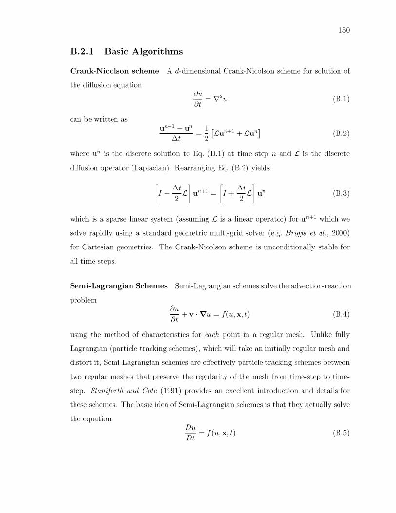
150
B.2.1 Basic Algorithms
Crank-Nicolson scheme A d-dimensional Crank-Nicolson scheme for solution of
the diffusion equation∂u
∂t= ∇2u (B.1)
can be written asun+1 − un
∆t=
1
2
[
Lun+1 + Lun]
(B.2)
where un is the discrete solution to Eq. (B.1) at time step n and L is the discrete
diffusion operator (Laplacian). Rearranging Eq. (B.2) yields
[
I −∆t
2L
]
un+1 =
[
I +∆t
2L
]
un (B.3)
which is a sparse linear system (assuming L is a linear operator) for un+1 which we
solve rapidly using a standard geometric multi-grid solver (e.g. Briggs et al., 2000)
for Cartesian geometries. The Crank-Nicolson scheme is unconditionally stable for
all time steps.
Semi-Lagrangian Schemes Semi-Lagrangian schemes solve the advection-reaction
problem∂u
∂t+ v · ∇u = f(u,x, t) (B.4)
using the method of characteristics for each point in a regular mesh. Unlike fully
Lagrangian (particle tracking schemes), which will take an initially regular mesh and
distort it, Semi-Lagrangian schemes are effectively particle tracking schemes between
two regular meshes that preserve the regularity of the mesh from time-step to time-
step. Staniforth and Cote (1991) provides an excellent introduction and details for
these schemes. The basic idea of Semi-Lagrangian schemes is that they actually solve
the equationDu
Dt= f(u,x, t) (B.5)

151
as an ordinary differential equation along the trajectory that connects from some
take-off point x∗ at time t to the regular grid point x at time t+ ∆t. In general they
can be written as
un+1 = un∗
+
∫ t+∆t
t
f (u(τ),x(τ), τ) dτ (B.6)
where un+1 is the solution on the regular grid at time step n+1. un∗
= un(t,x∗) is the
value of the solution at the take-off point (which is generally not on the grid). The
final term is the line integral of the source terms along the trajectory. The take-off
point x∗ is found by solving the ODE particle tracking problem
dx
dt= −v (B.7)
starting at the grid point x and moving back in time. Once the take-off point is lo-
cated, the value of the function and any attendant source terms are found at this point
by interpolation from the regular mesh un. Semi-Lagrangian schemes have consider-
able flexibility in their choice of particle tracking and interpolation schemes. We use
the simplest, second-order two-level scheme which uses an iterated mid-point scheme
to find the take-off point and bi-cubic interpolation (in 2-D) to interpolate values at
time step n (see Staniforth and Cote, 1991, for details). Lower order interpolants
such as bi-linear interpolation introduce systematic errors similar to the numerical
diffusion introduced by low-order up-wind schemes and are not acceptable. However,
higher-order interpolants can produce systematic overshoots near sharp edges that
remain localized to the edges but grow with time. Section B.5.1 describes a hybrid
interpolation scheme that preserves high-order interpolation for smooth fields but
prevents over-shoots near discontinuities.
To complete Eq. (B.6) requires an approximation to the final integral. For the
second-order two-level scheme we use a trapezoidal rule so that the full algorithm can
be written
un+1 = un∗
+∆t
2
[
fn∗
+ fn+1]
(B.8)
where fn∗
= f(x∗, t) is the value of the source term (usually interpolated) at the

152
take-off point.
For pure advection problems with no source terms, the Semi-Lagrangian scheme
reduces to un+1 = un∗, i.e. the value of the function remains constant on the charac-
teristic and the old value is simply copied into its new position on the regular grid.
As long as the take-off point and the old value can be found accurately, there is no
stability limit to the length of the time step. In practice, the second-order accuracy
of the mid-point scheme restricts the time step to ∼ 4 − 5 times the Courant num-
ber although for simpler flow fields, time steps greater than 10 times the Courant
condition are possible.
B.2.2 Hybrid Schemes
Given these two schemes for advection and diffusion, we combine them to solve the
scaled, constant diffusivity advection-diffusion problem
∂u
∂t+ v · ∇u = ∇2u (B.9)
where the maximum scaled velocity ||v||max is order the Peclet number, Pe = Lv0
κ.
Operator splitting OS-SLCN The first approach simply uses the Semi-Lagrangian
scheme to advect the quantity for a time ∆t such that un′
= un∗
and then diffuses for
a time ∆t using the CN scheme. The operator split semi-Lagrangian Crank-Nicolson
scheme for Eq. (B.9) is then
[
I −∆t
2L
]
un+1 =
[
I +∆t
2L
]
un′
(B.10)
Note that un′
has first been moved onto the regular grid before the diffusion
operator is applied. For small time-steps or for flows that do not significantly distort
gradients over a time-step, the operator split SLCN scheme can produce accurate
solutions for large time steps (see Section B.3). However, for strongly distorting
flows where advection and diffusion operate simultaneously, we find that a small

153
modification to this scheme is more reliable.
Operator Combined SLCN In the operator combined SLCN scheme, we consider
the problem slightly differently as
Du
Dt= ∇2u (B.11)
and treat it in the same manner as Eq. (B.5) with the diffusion as a “source term.”
Using the same discretization that leads to Eq. (B.8) we write the SLCN scheme as
un+1 = un∗
+∆t
2
[
(Lun)∗ + Lun+1]
(B.12)
where (Lun)∗ is the diffusion operator acting at the take-off point x∗ before advec-
tion has distorted the gradients. If L is the discrete Laplace operator and C∗ is the
bicubic interpolation operator at point x∗ then it is straightforward to show that on a
regular cartesian grid that the order of interpolation and diffusion is interchangeable
i.e. (Lun)∗ = LC∗un = C∗Lun. Thus, in practice, it is usually easier to apply the
Laplacian on the regular grid at time step n and then interpolate the resulting field.
With these definitions Eq. (B.12) can be rearranged to yield
[
I −∆t
2L
]
un+1 = un∗
+∆t
2(Lun)∗ (B.13)
or[
I −∆t
2L
]
un+1 = C∗
[(
I +∆t
2L
)
un
]
(B.14)
In the limit of no motion (Pe = 0 or v = 0), Eq. (B.14) is identical to a Crank-
Nicolson scheme (Eq. (B.3)) as C∗ = I (or un∗
= un and (Lun)∗ = Lun). It is less
obvious that in the limit of no diffusion (Pe → ∞), this scheme reduces identically
to the semi-Lagrangian scheme.
To see this, we first note that although none of these schemes have stability criteria,
we still have to choose a time step ∆t based on some accuracy criterion. For mixed
advection-diffusion problems we choose a time step based on the fastest process and

154
an accuracy criterion based on either the maximum number of grid points we want
to move in a time step or the smallest wavelength that we want to decay accurately.
For example we set
∆t = min
(
α∆x
||v||max
, (β∆x)2
)
(B.15)
where ∆x is a measure of the grid spacing, α is the maximum number of grid points
to move in a time step (i.e. the maximum Courant number) and λ = β∆x is the
minimum wavelength to resolve for diffusion at long times. In the limit of large
velocities (Pe → ∞), the time it takes to move α grid-points is negligible (i.e. ∆t =
O(ε)). In the limit ∆t → 0 Eq. (B.13) reduces to un+1 = un∗
which is just the
semi-Lagrangian advection scheme.
For strongly advectively dominated problems, it usually makes more sense to scale
by the advection time so that the dimensionless velocities are order 1, in which case
the problem becomesDu
Dt=
1
Pe∇2u (B.16)
and the combined SLCN scheme becomes
[
I −∆t
2PeL
]
un+1 = un∗
+∆t
2Pe(Lun)∗ (B.17)
and the Peclet number enters into the operator (thus the operator becomes poorly
scaled when the Peclet number is small and is singular for Pe = 0).
B.3 An analytic test problem
Strictly speaking, the method of characteristics does not work for advection-diffusion
problems because the diffusion operator moves information between particle trajec-
tories such that characteristics do not exist for all times. However, in practice, this
numerical scheme works well because it only considers the particle trajectories for a
single time-step and just provides a more accurate method to map a uniform grid
un at time t to another uniform grid un+1 at time t + ∆t. We have not proved this

155
0
0.2
0.4
0.6
0.8
1
1.2
1.4
1.6
1.8
2
amplitude=2.9373e−01
u(x, y, t=2.80 , Pe=8000 )
−6
−4
−2
0
2
4
6
x 10−3Residual, Uij−u
ij
0 0.5 1 1.5 2 2.510
−7
10−6
10−5
10−4
10−3
10−2
Time
% e
rror
Courant #=12.800
max resid: ||Uij−u
ij||
∞
/||Uij||
2×100
avg resid: ||Uij
||2/||U
ij||
2/(total # of nodes)×100−u
ij
(a) (b)
(c)
Figure B-1: Results of an example calculation using the combined operator SLCNscheme. (a) The u field at model time t = 2.8. (b) The residual, analytic minusnumerical, at the same time. (c) The residual over model time. The red curve showsthe maximum residual normalized by the L2 norm of the discrete analytic solution.The blue curve is the grid averaged L2 norm of the residual, normalized in the sameway.

156
rigorously, but provide a useful test of the algorithm for an analytic solution that
combines both advection and diffusion in a non-separable way.
This problem considers the solution of Eq. (B.9) in an infinite domain with velocity
field
v(x, t) = U(y) = Peyi (B.18)
and initial condition
u(x, 0) = eik·x (B.19)
Physically, this problem corresponds to advection-diffusion of a plane wave in a shear-
ing flow field (see Fig. B-1)
In the absence of diffusion, this problem can be solved by characteristics for any
initial condition u(x, 0) = f(x) such that u(x, t) = f(x − Peyt, y). In the case of a
plane wave initial condition, the solution is
u(x, t) = ei[kx(x−Peyt)+kyy] (B.20)
which can be written more physically as u(x, t) = eik(t)·x where
k(t) = kxi + (ky − kxPet)j
is a time dependent wave-number. Thus any initial plane wave remains a plane wave
but changes wavelength with time. For an initially vertical plane wave (ky = 0), shear
increases the wave-number with time and should enhance diffusion.
An analytic solution to the full advection-diffusion problem can be found by seek-
ing solutions of the form
u(x, t) = ei(k(t)·x)+s(t) (B.21)
Substituting Eqs. (B.18) and (B.21) into Eq. (B.9) and solving for s(t) gives
s(t) = −[
k2t− Pekxkyt2 + (Pekx)
2t3/3]
(B.22)
where k2 = k2x + k2
y. In the absence of advection (Pe = 0), this solution is simply

157
the exponential decay of a static plane wave. When Pe > 0 and initially ky = 0, the
shear enhances the decay rate of the amplitude as expected.
We test both the operator split and combined versions of the SLCN scheme
against the real part of this solution for a computational domain x ∈ [−1/2, 1/2], y ∈
[−1/2, 1/2]. Boundary conditions are periodic in the x-direction and dirichlet in y;
we prescribe the analytical solution at y = ±1/2 for all x. The initial condition that
we use is ky = 0, kx = 10π for five full cycles in the x-direction.
In addition to the two schemes described above, we also compare results with
numerical solutions using a Forward-time centered-space (FTCS) scheme as well as
a semi-implicit Crank-Nicolson centered-space (CNCS) scheme that discretizes the
advection term as
Pey∂u
∂x∼
Pey
2[un
i+1,j − uni−1,j] = Aun
and solves the linear system
[
I +∆t
2(A−L)
]
un+1 =
[
I −∆t
2(A−L)
]
un (B.23)
using a multigrid solver. The FTCS is a straw-man scheme: its CFL condition limits it
to very small time-steps and even under these conditions its accuracy and efficiency
are poor. The CNCS scheme is better than FTCS however it too has a stability
criterion that limits the time-step size.
B.4 Results
For each run of the benchmark problem we measure the process time (on a Sun Blade
100 with 250 KB RAM and a 500 MHz processor) and the accuracy of the solution.
Accuracy is measured by comparing the numerical solution to a discretized version
of the exact solution untrue:
% error =‖un
true − un‖2 or∞
‖untrue‖2
× 100 (B.24)

158
Figure B-1 shows the results of an example calculation using operator combined
SLCN. In this example the Peclet number is chosen to be 4000 and final shear strain
is .625. This combination of parameters results in the decay of the signal to 30% of
its initial amplitude. The L2 norm percent error is observed to parallel the infinity
norm in our calculations; for the rest of the paper, percent error is reported in terms
of the infinity norm.
Figure B-2 shows the comparison of accuracy as a function of Peclet number for
the SLCN scheme in operator split and combined versions with the CNCS scheme.
Each simulation is run to approximately one e-folding time in amplitude, thus the
amount of final shear increases with Peclet number. For small Peclet number, all
the schemes give the same results. This is as expected: they all reduce to pure
Crank-Nicolson for Pe → 0. For large Peclet number runs where final shear is higher
(advection is more important), SLCN performs better than CNCS, with a significant
advantage for the combined operator version of SLCN.
Figure B-3 shows the results of a set of simulations for different h and ∆t. It
is clear that even for time steps an order of magnitude longer, the SLCN schemes
perform significantly better than the other schemes. For example, in Figure B-3c,
with 12 grid intervals per initial wavelength and a Courant number of about 10, the
error is 0.03%, around an order of magnitude smaller than for the CNCS scheme can
achieve.
The computational time required for each of the calculations performed is shown
in Figure B-4. Computation time for the CNCS scheme and the SLCN schemes are
comparable for a given courant number. However, the SLCN scheme is stable to much
higher Courant number, so it is capable of accelerating the simulation significantly.
For the example given above, the SLCN scheme is about five times faster than the
CNCS scheme for an order of magnitude improvement in accuracy.
A comparison of operator split and operator combined SLCN shows that while the
operator combined SLCN scheme has a wide stability range where accuracy is approx-
imately constant, the operator split version has two regimes of accuracy dependence
on Courant number. In the first regime, at lower Courant numbers, the performance
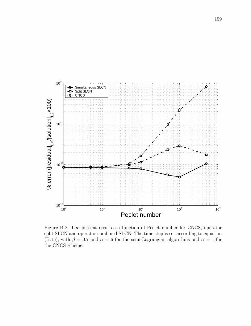
159
100
101
102
103
104
10−3
10−2
10−1
100
Peclet number
% e
rror
(|r
esid
ual| L∞
/|sol
utio
n|L2
×100
)
Simultaneous SLCNSplit SLCNCNCS
Figure B-2: L∞ percent error as a function of Peclet number for CNCS, operatorsplit SLCN and operator combined SLCN. The time step is set according to equation(B.15), with β = 0.7 and α = 6 for the semi-Lagrangian algorithms and α = 1 forthe CNCS scheme.
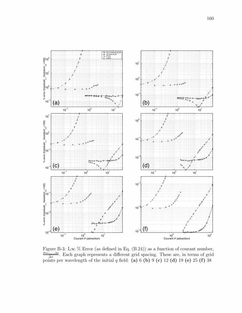
160
10−1
100
101
10−1
100
101
102
% e
rro
r (|
resid
ua
l|L
∞
/|so
lution
| L2×1
00)
Op Combined SLCNOp Split SLCNFTCSCNCS
10−1
100
101
10−1
100
101
10−1
100
101
10−2
10−1
100
101
% e
rro
r (|
resid
ua
l|L
∞
/|so
lution
| L2×1
00)
10−1
100
101
10−2
10−1
100
10−1
100
101
10−3
10−2
10−1
Courant # (advection)
% e
rro
r (|
resid
ua
l|L
∞
/|so
lution
| L2×1
00)
100
102
10−3
10−2
10−1
Courant # (advection)
(a) (b)
(c) (d)
(e) (f)
Figure B-3: L∞ % Error (as defined in Eq. (B.24)) as a function of courant number,Pevmax∆t
∆x. Each graph represents a different grid spacing. These are, in terms of grid
points per wavelength of the initial q field: (a) 6 (b) 9 (c) 12 (d) 19 (e) 25 (f) 38
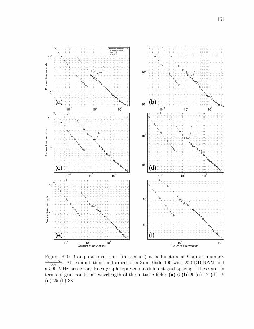
161
10−1
100
101
10−1
100
Pro
cess tim
e, seconds
Op Combined SLCNOp Split SLCNFTCSCNCS
10−1
100
101
10−1
100
10−1
100
101
100
101
Pro
cess tim
e, seconds
10−1
100
101
100
101
10−1
100
101
101
102
Courant # (advection)
Pro
cess tim
e, seconds
100
102
101
102
Courant # (advection)
(a) (b)
(c) (d)
(e) (f)
Figure B-4: Computational time (in seconds) as a function of Courant number,Pevmax∆t
∆x. All computations performed on a Sun Blade 100 with 250 KB RAM and
a 500 MHz processor. Each graph represents a different grid spacing. These are, interms of grid points per wavelength of the initial q field: (a) 6 (b) 9 (c) 12 (d) 19(e) 25 (f) 38

162
of the scheme improves with increasing time-step size. The second regime shows a
rapid degeneration of the performance as the time-step size continues to increase.
B.5 Discussion
The strengths of the shearing, diffusing plane wave as a benchmark problem are that
it couples advection and diffusion and that it has a non-separable analytic solution.
Our tests were successful in distinguishing the different schemes. The SLCN scheme
confers a significant advantage over the other schemes considered, both in terms
of accuracy and efficiency. The performance of the operator split SLCN scheme
compares favorably with the simultaneous operator version for some values of the
Courant number, but its accuracy is highly variable. We cannot explain this marked
variability.
There are limitations of the benchmark problem with respect to testing the SLCN
scheme. First, all advection is in one dimension and thus the calculated characteristics
are exact. A problem with a more complex flow field, e.g. curved particle trajectories
or stagnation points, would present a more demanding test of the SLCN scheme and
would degrade its accuracy at higher Courant numbers. Second, because character-
istics are parallel to the x-direction of the grid, interpolation is needed only in one
dimension (however computation times given above are for full bicubic interpolation).
A third limitation of the chosen benchmark problem is that the quantity being
transported varies smoothly in space. It is often necessary, in high Peclet number
advection-diffusion problems, to encounter shocks or fronts in the transported quan-
tity. A known problem with the semi-Lagrangian advection scheme arises under these
circumstances. The bicubic interpolant, chosen to reduce numerical diffusion with-
out incurring too great a computational cost, tends to overshoot near discontinuities
in the field. We have developed an adaptive interpolation method that retains the
advantages of bicubic interpolation while avoiding its associated overshoot problems.
To demonstrate this problem, and our solution, we performed a classic test of the
semi-Lagrangian advection scheme, solid body rotation of a square bordered with a

163
discontinuity.
B.5.1 Adaptive Interpolation Method
The adaptive interpolation method makes use of the fact that a bicubic interpolation is
executed by doing five cubic interpolations on four points each. Avoiding overshooting
on each of these five one dimensional interpolation steps is thus required for avoiding
overshooting in the overall bicubic interpolation.
In constructing the one dimensional cubic overshoot detection algorithm we make
the assumption that the field is sufficiently well resolved on the grid that there are
no oscillations at the grid scale. Thus we expect that over a set of four points, the
first derivative of the field can change signs at most once. Given a set of field values
yi with local index i ∈ 0, 1, 2, 3 and a real-valued interpolation target in local grid
coordinates x = i∆x, 1 ≤ x ≤ 2, we detect an overshoot using the following steps:
1. For each i, compute the slope, y′i, of the cubic interpolant at x = i∆x.
2. There are oscillations in the interpolant over the grid segment if SIGN(y′3) equals
SIGN(y′0) and SIGN(y′2) does not equal SIGN(y′3).
Because this test is fairly expensive, it is performed only if the set of points y
meets two conditions. First, the absolute range of y must be greater than a specified
fraction of the range in values over the whole domain. If the set of interpolation points
is constant to a within this fraction it may still have features in the noise that cause
detectable but small overshoots that do not damage the solution. Second, the cubic
interpolant must fall outside of a specified envelope around the linear interpolant.
This envelope is defined by a tolerance on the normalized difference between the
cubic and the linear interpolants, as shown in Figure B-5.
The results of the solid body rotation test are shown in Figure B-6 for three full
rotations around a corner of the box. The overshoots evident in the pure bicubic
interpolation run are suppressed by the adaptive interpolation method. Bilinear in-
terpolation is included for comparison (but tends to show large amounts of numerical
diffusion)..

164
0 1 2 30
0.2
0.4
0.6
0.8
1
1.2
1.4
Local grid index
(y−
min
(yi))
/ (
ma
x(y
i)−m
in(y
i))
Scaled y valuesLinear interpolantCubic interpolantTolerance envelope (exaggerated)Interpolated value
0 1 2 30
0.2
0.4
0.6
0.8
1
1.2
1.4
(y−
min
(yi))
/ (
ma
x(y
i)−m
in(y
i))
(a)
(b)
Figure B-5: Two examples of adaptive interpolation with overshoot detection, bothwith x = 1.3. The green lines delineate the tolerance envelope, the thickness ofwhich is exaggerated for clarity. (a) In this case, assuming that the field is smooth,the cubic interpolant is a better approximation than the linear one. The overshootdetection algorithm correctly returns false. (b) This figure shows the overshoots thatcharacterize the cubic interpolant near an edge. The overshoot detection algorithmreturns true and thus the linear interpolant is chosen.

165
5 10 15 20 25 30 35 40 45 5010
20
30
40
50
0
0.1
0.2
0.3
0.4
0.5
0.6
0.7
0.8
0.9
1
Analytic
5 10 15 20 25 30 35 40 45 5010
20
30
40
50
0
0.1
0.2
0.3
0.4
0.5
0.6
0.7
0.8
0.9
Bilinear
5 10 15 20 25 30 35 40 45 5010
20
30
40
50
0
0.1
0.2
0.3
0.4
0.5
0.6
0.7
0.8
0.9
1
Bicubic
5 10 15 20 25 30 35 40 45 5010
20
30
40
50
0
0.1
0.2
0.3
0.4
0.5
0.6
0.7
0.8
0.9
1
Adaptive
10 20 30 40 50 60 70 80 90 100
0
0.1
0.2
0.3
0.4
0.5
0.6
0.7
0.8
0.9
1
Array index
z
AnalyticBilinearBicubicAdaptive
(a) (b)
(c) (d)
(e)
Figure B-6: Results for three interpolation methods for the semi-Lagrangian ad-vection scheme, compared with the analytic solution after three full rotations. (a)Analytic solution. (b) Bilinear interpolation (c) Bicubic interpolation (d) Adaptiveinterpolation. (e) Profiles across the box after 1 (solid line), 3 (dashed line) and 9(dash-dotted line) full revolutions.

166
B.6 Conclusions
A general numerical solver for advection-diffusion problems must be capable of han-
dling pure advection, pure diffusion and any combination of the two. The accuracy
and stability of such a solver becomes especially critical in the case of advectively
dominated problems with sharp spatial gradients in the transported quantity. The
SLCN algorithm draws on the strengths of the Crank-Nicolson scheme for diffusion
and the semi-Lagrangian scheme for advection. Since neither of these have time-steps
limited by a stability criterion, the SLCN scheme is also unconditionally stable. We
have shown that when the advection and diffusion operators act simultaneously on
the transported field the SLCN scheme is accurate and efficient over a broad range
of time step sizes relative to two other advection-diffusion schemes. Furthermore, by
employing our adaptive interpolation method, the SLCN scheme is able to handle
discontinuities while reducing the problems of cubic interpolant overshooting, and
maintaining its low numerical diffusivity.