the dlr visualization library...the dlr visualization library recent development and applications...

The DLR Visualization LibraryRecent development and applications

Matthias Hellerer Tobias Bellmann Florian SchlegelGerman Aerospace Center (DLR), Institute of System Dynamics and Control

82234 Wessling, Germany

Abstract

Modelica models are mathematical descriptions andtherefore their simulation output typically shows nu-merical variable trajectories. While universal for allkinds of simulations, this representation is oftentimesdifficult to understand. In the field of multi-body sim-ulations, 3D visualizations present a way of display-ing vast amounts of numerical data in an intuitiveway which is instantly understandable, even by peo-ple without specialized knowledge. For integrationof visualization in Modelica multi-body simulations,the "DLR Visualization Library" has been developed.This paper presents the newest additions to the libraryand shows their application in several DLR projects.

Keywords: Visualization, Simulation, DLR Visual-ization Library, Modelica, interactive Simulation

1 Introduction

The visualization of simulation data is an important el-ement of advanced simulations. With the increasingcomplexity of modern multi-body simulations, con-cerning for example flexible bodies, thermal dissipa-tion, or contacts, the demands for a realistic, real-timecapable visualization of the simulation also rise. Us-ing Modelica as modeling language allows the userto pack model functionality in reusable sub-models,e.g. as a replaceable block for a suspension, an engine,etc. This also enables the integration of visualizationdefinitions into the single sub-models, eliminating theneed for an additional visualization definition in a sep-arate program.

In 2009, the "DLR Visualization Library" for Mod-elica has been introduced under the now deprecatedname "DLR External Devices Library" [1]. The li-brary features a variety of visualization blocks to beused directly as visualizers within Modelica. Visu-alization elements like configurable rigid bodies (e.g.

sphere, box, gearwheel) or rigid and flexible bodiesgenerated from CAD files can be displayed by con-necting their respective Visualizer block to the cor-responding frame in the multi-body model. Figure 1shows an example scene created in Modelica and itsvisualization. Using the C-interface of Modelica, thevisualization information is transmitted to the externalvisualization software which is started automatically

Figure 1: Top: Modelica model for a single cylinder,showing the integration of model and visualization.Bottom: The corresponding 3D visualization of a ra-dial engine.

DOI10.3384/ECP14096899

Proceedings of the 10th International ModelicaConferenceMarch 10-12, 2014, Lund, Sweden

899

with the simulation and allows the user to replay andobserve the simulation run in real-time and export it asvideo. Furthermore, as a result of the latest develop-ment, the library features a feedback channel, allow-ing the visualization to influence the simulation. Thismakes it possible to interact with the simulation us-ing a graphical user interface (GUIs / HUDs), definedin the Modelica model, and to evaluate collisions be-tween visualization elements, this is for example re-quired in contact force calculations.

The following sections shall introduce the newlyadded features to the "DLR Visualization Library" andpresent some application examples of its use in ongo-ing research topics at DLR.

2 State of the art

The first attempts to create 3D Visualizations withModelica was in 2000, when Engelson [2] started adiscussion about techniques for the integration of vi-sualization information with Modelica code. In hispaper he presents a set of annotations for 3D graphicprimitives and standardized simple geometries. Visu-alization would then have to be implemented by IDEtool vendors. Even though it brought up the idea ofcreating visualizations from Modelica models, the pre-sented techniques were never implemented on a largerscale.

Yet, the idea of creating 3D visualizations fromModelica simulations persisted and in 2003 Otter etal. [3] revived the "MultiBody Library" of the Model-ica standard library. This change introduced a new sublibrary called "Visualizers", containing shape objectsfor simple 3D forms as well as more complex objectsfrom files. These are Modelica blocks and as such mayeasily be integrated in existing models or may be usedin the creation of submodels which contain both simu-lation and visualization information. The visualizationitself is redirected to the ModelicaServices library, re-sponsible for all vendor specific implementations. Sothe Modelica standard library provides a standardizedvisualization description, to be implemented by Mod-elica IDE vendors. This technique is now part of allmajor simulation environments.

In 2008 Hoeft et al. [4] revisited the ideas of Engel-son, this time integrating the powerful X3D standardin Modelica annotations. X3D, short for Extensible3D Graphics, is an open international standard, devel-oped for web applications. It is a representation of a3D environment with XML. They present new annota-tions with X3D code and show an implementation of

the technique in the MOSILAB simulator.Furthermore the Modelica3D library was presented

by Höger et al. at the 2012 Modelica Conference [5].It implements a scene graph in Modelica and uses theC-interface to connect the simulation front-end withthe visualization back-end via interprocess communi-cation. Besides their Modelica library, two differentback-ends are presented. One based on the Open-SceneGraph 3D library and one based on the Blender3D graphics software.

Unsatisfied with the existing visualizers, providedby "MultiBody Library", we implemented the "DLRVisualization Library". It is based on the ideas of En-gelson and Otter, but tries to take those to the next levelwith more complex 3D environments, visualizations ofmass and power flow, flexible deformation of objectsand many other features in a high fidelity rendering.

3 New Functions

3.1 3D-Elements

3.1.1 Dynamic textures

Given a 2D Matrix of 3D points, the flexible surfaceelement may be used to display arbitrary shapes, withthe ability to deform during the simulation. More de-tails may be found in [1].

A new addition to flexible surfaces is the ability todisplay videos as textures, both local files as well asvideo streams from a network, as shown in figure 2.For local files the video is synced with the simulationtime stamp. For network streams this is not possibleand the surface will always display the last receivedimage. The supported network protocols and the URLdefinitions for opening streams are inherited from theunderlying FFmpeg library and are described in [18]in detail. Most commonly used protocols are therebysupported, such as: RTP, FTP, MMS, HTTP and HLS.

Figure 2: Full HD MPEG Video image from a pre-sentation of the DLR Robotic Motion Simulator [9],rendered onto a flexible surface.

The DLR Visualization Library - Recent development and applications

900 Proceedings of the 10th International ModelicaConferenceMarch 10-12, 2014, Lund, Sweden

DOI10.3384/ECP14096899

Figure 3: On the left a simple 3D scene; on the rightthis part is rendered on a flexible surface using a virtualcamera, symbolized on the upper left side. All partsare in the same scene.

Besides Videos, images from virtual cameras canbe rendered onto a flexible surface. For this purposea standard camera from the "DLR Visualization Li-brary" is placed in the scene and its output mode is setto "render to texture". The camera output can then beselected as texture for the flexible surface. The resultis a camera image, drawn on the surface in the sameway it would otherwise be drawn on screen. An exam-ple of this is illustrated in figure 3. The whole imageshows one scene. On the left side a few objects arearranged and on the right side a flexible surface is de-picted which shows the left part of the scene again, asseen from the virtual camera above the arrangement,rendered as a texture on a flexible surface.

3.1.2 Feedback - HUD

In [1] all communication was strictly from the sim-ulation to the visualization. The following, new ele-ments abandon this concept. They not only send datafrom the simulation to the visualization but also re-ceive data, which may then be used to influence thesimulation.

The first interactive objects presented here are inter-active HUD elements. The base class for all of theseelements is the button class. This defines an invisi-ble HUD object in the visualization and with outputsin the simulation which are dependent on user inputon the visualization. By combining the button objectwith HUD elements for the representation and Model-ica logic for reactions, typical user interfaces, like but-tons or sliders, can be created and used as interactiveinput for simulations. The button base class is capa-ble of reacting to mouse-over events while the mousecursor hovers over them, mouse clicks and draggingof the element by moving the mouse while a button

Figure 4: At the top part simple HUD elements arepresented and below that their representation in theModelica graphical designer.

is clicked. The "DLR Visualization Library" containswith a selection of predefined GUI elements, using thedescribed button base class. The following HUD ele-ments are depicted in figure 4:

• Buttons are by default visualized as simplesquares with a label. They have a Boolean out-put value which is "true" for as long as the userpresses it and "false" otherwise.

• Check boxes have a different look but actuallybehave very similar to buttons, except the out-put value behaves like a flip-flop. Permanentlychanging its value with every click.

• Sliders for simple adjustment of continuous val-ues

3.1.3 Feedback - Collision detection

The description of complex 3D geometries usuallyuses geometric meshes. Reading the according datafrom files, interpreting it and running collision detec-tion algorithms from Modelica is complicated. Phys-ical simulations, especially in the area of multi bodysimulations often require to measure the distance be-tween objects or contacts between objects. The re-quired data, especially the interpretation and arrange-

Session 5E: Modelica Tools 3

DOI10.3384/ECP14096899


901

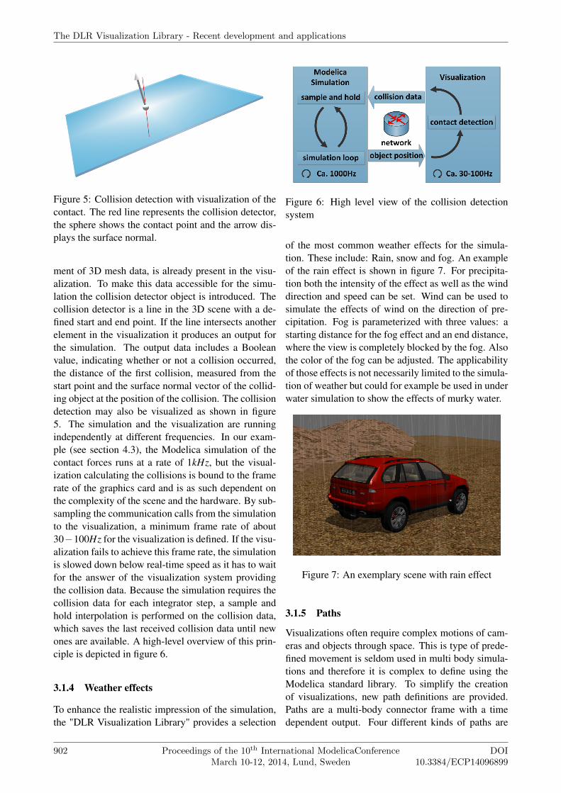
Figure 5: Collision detection with visualization of thecontact. The red line represents the collision detector,the sphere shows the contact point and the arrow dis-plays the surface normal.

ment of 3D mesh data, is already present in the visu-alization. To make this data accessible for the simu-lation the collision detector object is introduced. Thecollision detector is a line in the 3D scene with a de-fined start and end point. If the line intersects anotherelement in the visualization it produces an output forthe simulation. The output data includes a Booleanvalue, indicating whether or not a collision occurred,the distance of the first collision, measured from thestart point and the surface normal vector of the collid-ing object at the position of the collision. The collisiondetection may also be visualized as shown in figure5. The simulation and the visualization are runningindependently at different frequencies. In our exam-ple (see section 4.3), the Modelica simulation of thecontact forces runs at a rate of 1kHz, but the visual-ization calculating the collisions is bound to the framerate of the graphics card and is as such dependent onthe complexity of the scene and the hardware. By sub-sampling the communication calls from the simulationto the visualization, a minimum frame rate of about30−100Hz for the visualization is defined. If the visu-alization fails to achieve this frame rate, the simulationis slowed down below real-time speed as it has to waitfor the answer of the visualization system providingthe collision data. Because the simulation requires thecollision data for each integrator step, a sample andhold interpolation is performed on the collision data,which saves the last received collision data until newones are available. A high-level overview of this prin-ciple is depicted in figure 6.

3.1.4 Weather effects

To enhance the realistic impression of the simulation,the "DLR Visualization Library" provides a selection

Figure 6: High level view of the collision detectionsystem

of the most common weather effects for the simula-tion. These include: Rain, snow and fog. An exampleof the rain effect is shown in figure 7. For precipita-tion both the intensity of the effect as well as the winddirection and speed can be set. Wind can be used tosimulate the effects of wind on the direction of pre-cipitation. Fog is parameterized with three values: astarting distance for the fog effect and an end distance,where the view is completely blocked by the fog. Alsothe color of the fog can be adjusted. The applicabilityof those effects is not necessarily limited to the simula-tion of weather but could for example be used in underwater simulation to show the effects of murky water.

Figure 7: An exemplary scene with rain effect

3.1.5 Paths

Visualizations often require complex motions of cam-eras and objects through space. This is type of prede-fined movement is seldom used in multi body simula-tions and therefore it is complex to define using theModelica standard library. To simplify the creationof visualizations, new path definitions are provided.Paths are a multi-body connector frame with a timedependent output. Four different kinds of paths are



DOI10.3384/ECP14096899

Figure 8: Top to bottom: circular, linear, Bezier, cubicspline; spheres: control points.

available as shown in figure 8: The first type shownhere is a circular movement. The circle is defined bya center point with orientation and the radius. Thesimplest paths are point to point connection. A listof points is supplied and the resulting path is a lin-ear interpolation between those. For smoother paths,Bezier curves can be used. The path is only guaranteedto pass through the first and the last point the remain-ing points only "stretch" the path towards them. Thefourth kind of paths is based on cubic spline interpo-lation. Like Bezier curves these provide very smoothpaths. In contrast those the line is always guaranteedto pass through all points. This often simplifies thedefinition of paths but might lead to overshooting incertain constellations.

3.1.6 Trace shape

Following the 3D movement of multiple objects atonce can be hard. To display this motion, a trace-shapecan be attached to any object. The trace-shape objectthen generates a line trail as the object it is attached tomoves through space, thereby intuitively representingthe objects trajectory. For the illustration of multipletrails, the line thickness, color and length can be ad-justed by the user as needed. An example can be seenin figure 9.

3.1.7 Sky-Box

"Empty" space, areas on screen in which no object isdefined, are by default filled with a solid color. This issuitable for small animations or abstract illustrationsbut for many applications a more realistic represen-tation is required. For example in outdoor scenariosthose areas should show the horizon and the sky. Forthis purpose the sky box is introduced. The sky box

Figure 9: Movement of a robots tool tip visualized us-ing the trace shape.

is always depicted as infinitely far away and is com-posed of two layers. The front layer is used for dis-playing some sort of horizon. An example would bedistant hills or a tree line. The user has to supply siximages (It is designed as a cube with the view pointin the middle. One image per side). Behind this layer,visible through transparent areas in the images, the skyis drawn. The user has to provide a date, the time anda position on earth in form of longitude and latitude.The OsgEphemeris library [13] then uses this infor-mation to calculate the correct position of the sun andthe moon during the day and an astronomically correctstar field during the night time. The result is a realisticbackground for the simulation.

3.1.8 Particle System

The particle system is used for displaying objects, con-sisting of many sub-objects and cannot be modeled astraditional meshes. Examples for these kinds of ob-jects include streams of water, fire, smoke and dis-persed dust. Those objects are visualized using a largenumber of small objects, showing a simple image,called particles. Those particles are send out randomlyfrom an emitter, follow a certain path while poten-tially turning, changing color and transparency, untilthe path reaches a certain length and the particle dis-appears. Using the right image, a large number of ob-jects, and a specific movement, this raises for examplethe impression of water flowing from a pipe.

The Modelica blocks for modeling particles are di-vided by emitter type. The emitter is the area, fromwhich the particles are shot. The three types availablein the "DLR Visualization Library" are: Point emitter,


DOI10.3384/ECP14096899


903

Figure 10: Top: Three types of particle emitters. Fromleft to right line emitter (along z-axis), point emitter,and area emitter (circular shape in x− z-plane);Bottom: Particle effects used to display exhaust froma space rocket.

line emitter and area emitter. Examples for each typeare depicted in figure 10. The particles are created ran-domly within certain bounds, such as mean numberof particles per second, configurable for each emitter.Furthermore the particle may change its color, trans-parency, size over its life time. The final set of param-eters then determines the path particles will follow.

3.1.9 Virtual Planet Builder and large scale ter-rain visualization

The visualization engine is based on the open sourcelibrary OpenSceneGraph [12], allowing its use in con-junction with another OpenSceneGraph application,which is itself not part of the library: Virtual PlanetBuilder [14]. Using digital elevation data, like itis commonly produced in aerial surveys with spe-cial cameras, Virtual Planet Builder can produce 3Dsceneries at scale of whole planets. This is accom-plished by auto generating different levels of detailand by converting the scenery in a special file format.The planet surface is tiled into junks. When viewedfrom a faraway distance large areas are combined into

one large tile with very little detail. As the cameramoves closer to a certain area the corresponding tile issplit into smaller junks with more detail. This processis reiterated while the camera closes in until a maxi-mum degree of detail is reached. For the viewer theswitchover is not visible for the lower level detail atwhich a tile is rendered from afar, is not visible. Ofspecial importance is the way the data is preprocessedand stored in a special format, allowing the renderer toload certain parts at different levels of detail as needed,very efficiently. This technique makes it possible toshow extremely large areas while retaining a high levelof detail. Figure 11 shows an earth model, created withVirtual Planet Builder from satellite images.

When rendering these planetary scale images inconjunction with small, close up objects, in setups likethe satellite simulation in figure 11, graphical glitchesappear. During the rendering process, each pixel is as-signed a depth value to determine how objects overlapeach other from the cameras perspective. The techni-cal implementation of this uses a so called depth bufferor z-Buffer which safes each pixel distance from thecamera (the depth or z-value). This is a, typically 24-bit on modern machines, fixed point value in the range[0,1], where 0 represents the near plane (minimum dis-tance from camera) and 1 the far plane (maximum dis-tance) of the view frustum. Therefore, with increas-ing distance between the near and far plane, the depthbuffer resolution decreases. When the depth value oftwo points is so small that the depth buffer is unableto represent the difference graphical glitches becomevisible [15]. The minimum depth difference repre-sentable by the depth buffer ∆zmin can be calculatedwith equation (1). z is the depth value, n is the near

Figure 11: A model of planet earth, generated us-ing virtual planet builder, in a satellite simulation;Logarithmic Z-Buffering allows for a detailed satel-lite model in the foreground and an earth model at realscale behind it.



DOI10.3384/ECP14096899

plane distance and b is the depth buffers resolution inbit. The higher resolution at low distances is causedby perspective effects.

∆zmin ≈z2

2bn− z(1)

Logarithmic depth buffers are a well known techniquewhich seeks to attenuate this problem by applying alogarithm to the depth value before it is written tothe depth buffer, thereby increasing the resolution forclose objects, where small difference are more likelyto be important at the expense of the resolution fordistant objects where small differences are less likelyto become visible. Equation (2) show the conversionfrom the original value z to the new value zlog. The ad-dition parameter C is used to adjust whether close ordistant objects are preferred.

zlog =2ln(Cz + 1)

C f + 1−1 (2)

Using a logarithmic depth buffer alters the depth bufferresolution. It can now be calculated with equation (3).[16]

∆zlogmin ≈ln(C f + 1)

(2b−1) CCz+1

(3)

For example, the satellite visualization requires arender distance of 1m to 15000km. With a 24bit depthbuffer this results in a minimum depth separation ofless than 1mm at the satellites distance of 100m, butbetween ≈ 550m and ≈ 1100km at the earths distanceof 300km− 13000km, causing visible problems withits rendering. Using logarithmic depth buffers with aC Value of 0.001 the minimum separation for the satel-lite also lies below 1mm, yet for earth it is in the rangeof about ≈ 20cm−7.5m which is well below the visi-ble range at this distance.

3.1.10 Oculus Rift Integration

The Oculus Rift is head-mounted virtual reality dis-play, currently under development by Oculus VR. Atthe time of this paper, it is only available as a devel-oper preview version with a finalized consumer prod-uct in development. The head-mounted system de-picted in figure 12 includes a display with a resolutionof 1280× 800, two fish eye lenses stretching the im-age to a field of view of about 90 ◦−110 ◦ and a threedegree of freedom rotational acceleration sensor [17].With this device it is possible to generate a fully im-mersive experience in a 3D environment, nearly fillingthe user’s entire field of view and following his mo-tion as he moves his head. The "DLR Visualization

Figure 12: The Oculus Rift head-mounted virtual real-ity device.

Library" supports the currently available Oculus RiftDevelopment Kit as alternative display device for anykind of already integrated cameras. All setup steps andthe camera orientation change as reaction to the usershead movement are handled fully automatically.

3.1.11 HUDs

Head-Up-Displays are a two dimensional layer in frontof the three dimensional scene. The possible applica-tions for this kind of display range from overlaying lo-gos, over the display of model state variables to com-plex interactive user interfaces. All user interfaces arecomposed of five base elements: The first element istext. Text can change dynamically and therefore beused to display model states or variables. Also typ-ical text formatting methods such as different fonts,bold text and so on are supported. The second typeof elements is a line drawn along a list of user pro-

Figure 13: Various HUD elements used to recreate aplane’s cockpit instrumentation with artificial horizon,speed and altitude meters alongside a compass and en-gine status displays.


DOI10.3384/ECP14096899


905

vided points. Next are free form faces, displaying afilled form based on polygon points provided by theuser. Lastly, for more complex images, graphics filescan be included. Of course the HUD elements pre-sented here can be combined in the creation of newmore complex elements. A small selection of such el-ements is included with "DLR Visualization Library".An example is a scope for the presentation of variabletrajectories, a combination of lines, images and text, orthe airplane cockpit instrumentation in figure 13. Thelast type is an interactive button base class which willbe discussed in a later section.

Attention has to be paid to the arrangement of HUDelements for the size of the window they are drawn isvariable even at runtime. Therefore it would be im-practical to use absolute coordinates and instead rela-tive coordinates are employed. For the adaptation toa changed display size the user can choose of the fol-lowing four techniques:

1. The horizontal coordinate value spans over thehorizontal display size and the vertical value isadjusted to its size is such a way that aspect ratiois preserved.

2. The same as 1 but for the vertical instead of thehorizontal coordinate value.

3. The program automatically changes betweentechnique 1 and 2, depending on the smaller side.

4. Relative coordinates range for both horizontaland vertical coordinates range over the whole dis-

Figure 14: The "DLR Robotic Motion Simulator"

play size. The aspect ratio might be distorted de-pending on the display window setup.

4 Applications

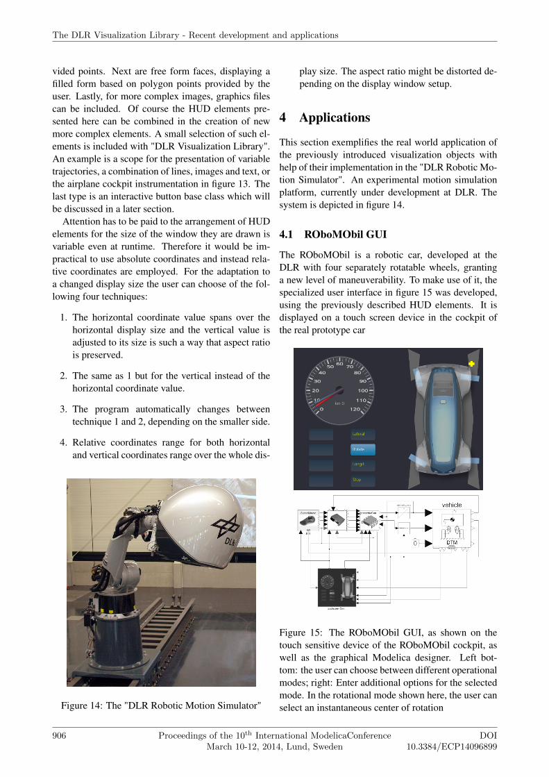
This section exemplifies the real world application ofthe previously introduced visualization objects withhelp of their implementation in the "DLR Robotic Mo-tion Simulator". An experimental motion simulationplatform, currently under development at DLR. Thesystem is depicted in figure 14.

4.1 ROboMObil GUI

The ROboMObil is a robotic car, developed at theDLR with four separately rotatable wheels, grantinga new level of maneuverability. To make use of it, thespecialized user interface in figure 15 was developed,using the previously described HUD elements. It isdisplayed on a touch screen device in the cockpit ofthe real prototype car

Figure 15: The ROboMObil GUI, as shown on thetouch sensitive device of the ROboMObil cockpit, aswell as the graphical Modelica designer. Left bot-tom: the user can choose between different operationalmodes; right: Enter additional options for the selectedmode. In the rotational mode shown here, the user canselect an instantaneous center of rotation



DOI10.3384/ECP14096899

and in the simulators cockpit mockup. The conceptis explained at full detail in [8]. The upper left partshows the current and the target speed. Below thatthe driving mode can be selected and the right part isselecting a rotation center point, required for certaindriving modes. The second part of this image showsthe full integration of the GUI with other parts of thesimulation directly in the model description with Mod-elica.

4.2 Flexible trajectory planning

The design of a complex trajectory in 3D space, for apredefined movement of objects or cameras, can be arather difficult and time consuming task, if it has to beaccomplished by the direct manipulation of numericparameters. Therefore the interactive Trajectory De-signer has been developed to provide a convenient wayof creating control point parameters for a B-spline in-terpolated movement of position and orientation. Thetrajectories velocity is interpolated with a two timesderivable sinusoidal function.

In order to generate a smooth trajectory through ac-curately defined bases containing a position and ori-entation, we use quaternions for orientation and B-Splines for interpolation between these bases. A B-Spline curve T (x) consists of control points Pi, i ∈1 . . .n − p and B-Spline base functions Ni,p,τ , i ∈1 . . .n− p−2:

T (x) =n−p

∑i=1

PiNi,p,τ (x) . (4)

The control points Pi each contains seven elements;three for position and four for the orientation repre-sented as quaternion. A base function Ni,p,τ is definedas a polynomial piece with order p and knot vector τ:

Ni,0,τ (x) :={

1, x ∈ [τi,τi+1 [0, otherwise

(5)

Ni,p,τ (x) = x−τiτi+p−τi Ni,p−1,τ (x)

+τi+p+1−x

τi+p+1−τi+1 Ni+1,p−1,τ (x) p> 0(6)

The knot vector τ = [τ0, . . . ,τn−1]T ,n ≥ 2p,τi ≤τi+1 and τi ≤ τi+p has to be chosen. The algorithmsof our implementation set the first and last p knotsequal. There are different approaches setting the re-maining values, see [11] [10, p161]. For the traje-tory designer we use a base functions with degree 3in order to get a smooth trajetory with a continuity ofthe second derivative. The parameter x defines the po-sition on the trajectory, T (x) returns the interpolated

value P(x) containing the three-dimensional positionand an interpolated quaternion. The quaternion inter-polation corresponds to a linear quaternion interpola-tion (LERP)[6]. Therefore the resulting L2-Norm ofthe vector is less than 1 and has to be normalized re-sulting in a unit quaternion which leads to an varyingbut continuous rotational velocity. Furthermore thetrajectory designer provides the functionality to set avelocity at each control point. The behavior of the ve-locity between the points is computed through sinu-soidal functions:

v(λ ) = (λ − 12

π sin(2πλ ))(vi+1− vi)+ vi; (7)

with vi the velocity of the left and vi+1 the veloc-ity of the right control point within the interval be-tween Pi and Pi+1. The second derivative of this si-nusoidal function is continuous and zero at the leftand right end providing a smooth transition at the con-trol points. The integration of the velocity v leads tothe current position on the trajectory x. Therefore,vi ≥ 0, i ∈ 1 . . .n− p.

The tool is operated by a small selection of key-board commands and offers three operating modes tomanipulate the position, the orientation and the asso-ciated velocity of the control points. In all modes con-trol points can be removed or inserted. For verificationof the resulting interpolated movement a live preview,adjusting to the manipulation of control points in real-time, is available. The preview shows a coordinate sys-tem traveling along the spline in the main scene and

Figure 16: The trajectory designer tool showing a path(green line) above Mt. Everest. In the upper right cor-ner a window previews the camera’s trajectory whileworking on it.


DOI10.3384/ECP14096899


907

a point of view rendering, adequate for the previewof camera movements, in a separate picture-in-picturepreview area. The complete interface is depicted infigure 16. The coordinates, orientations and velocitiesare finally stored as vectors in a text file, which can beused to reload the control points for further manipula-tion or later playback.

4.3 Wheel ground contact

The simulation of cars requires the modeling of con-tacts between wheels and the ground, realized usingthe collision detector elements. An abstracted modelis shown in figure 17. This contact model is then thebasis for far more complex models, such as the carshown in figure 18. In this simulation the load on thewheels will shift when driving on uneven terrain andthe suspension reacts accordingly. The ground planein the simulation can be any 3D shape.

The wheel vertical force is calculated according tothe following equation. The contact force f is the sumof a spring force s and a damping force d.

~f =~s + ~d (8)

The spring force is calculated using the penetrationdepth of the collision object and an other object p, aswell as a spring constant provided by the user S, topush the wheel away from the other object, along the

Figure 17: Wheel ground contact in the graphicalModelica designer and as 3D visualization.

Figure 18: A car driving on a plane. White arrowsindicate surface normals for contact points.

objects surface normal at the point of contact.

~s = S · p ·~n (9)

Just using a spring force would result in a constantlybouncing wheel. To model energy dissipation, a damp-ing force d is introduced. It is calculated using thecollision objects speed r in the direction of the surfacenormal n, a user provided damping constant D and theresulting force, just as the spring force, acts in the di-rection of the normal. Lastly the damping force shouldonly be present during impact. Otherwise the wheelwould act as if it was glued to the surface.

~d = D ·min(0,~r ·~n) ·~n (10)

This way of simulating object collisions does comewith certain draw backs. First of all, it intrinsicallyrequires the two colliding objects to interpenetrate.While problematic for rigid bodies, it is a reasonableapproximation for flexible objects like the car tires inthe presented example. When trying to minimize theinterpenetration a further problem arises. The largerthe spring constant s, the stiffer the simulation gets,requiring ever smaller simulation time steps. Other-wise the interpenetration from one step to the nextcan be so large, the resulting force from equation (9)gets unrealistically large, hurling the wheel away. Thesame problem can occur when the wheel is movingwith high speed and the ground inclination changes.The sample-and-hold technique used in the communi-cation, delays the point in time when the simulationis able to "see", the changed ground inclination. Thisis depicted in figure 19. The wheel on the left movesat high speed to the right but due to the slower visu-alization time steps, the ground inclination change iscommunicated to the simulation with delay, causingthe wheel to penetrate the ground.



DOI10.3384/ECP14096899

Figure 19: Wheel moving at high speed from left toright. Due to the fact that the simulation does run fasterthan the visualization, the inclination change is recog-nized to late. Dotted line: ground level as detected bythe simulation; red line: error due to sample and holdtechnique

For small and fast moving objects, it is even possi-ble for object collisions to be missed completely. Thecollision detection object only detects collisions withobject surfaces so if an object moves so fast towardsan other, that the position "jump" between time stepsis larger than the collision object length, the collisionmight get missed. This case is described by equation(11) where v1 and v2 the speed of the two objects andi1 and i2 are start and end point of the collision object.

∣∣∣∣∣∣∣∣

v1− v2

||v1− v2||· i1− i2||i1− i2||

∣∣∣∣∣∣∣∣

1f> ||(i1− i2)|| (11)

4.4 Image warping

The capsule in figure 20 is part of a simulator project.At the back, besides the head of the pilot, are two pro-jectors. The projection screen is the open capsule shellto the top right. The shell has a complex geometry,deforming the images projected onto it. In order topresent a rectified image to the pilot a reverse defor-mation has to be applied to the image prior to projec-tion. This preprocessing utilizes the render image totexture functionality on a flexible surface. Due to thefact that a flexible surface is used, the image can bewarped as needed (see figure 20) and with the correctconfiguration, the final image appears restituted to thepilot.

4.5 Manned vehicle simulation

The "DLR Robotic Motion Simulator" uses the cap-sule shown in figure 20 and an industrial robot towhich the capsule is attached as shown in figure 14.The robot is then used to apply accelerations, in accor-dance with the simulation, on the pilot, thereby creat-ing an immersive motion simulation. A detailed de-scription of the "DLR Robotic Motion Simulator" can

Figure 20: The piloting capsule of the "DLR RoboticMotion Simulator"; On top the stereo images afterwarping; The images are projected on the capsule andappear restituted; In front of the pilot is a touch sensi-tive display.

be found in [7]. In this application all of the previ-ously shown applications are utilized. The pilots’ mainscreen is restituted using the render to texture featureon a flexible surface; the console in front of the pilotshows an input GUI on touch screens, and the vehi-cle simulation uses collision detection objects for thewheel ground contact analysis.

5 Limitations

The presented library does have certain limitations inits current state, of which the following three are cur-rently under investigation for improvements. The firstone is the design of the collision detection system: itonly allows for collisions with a line object, limitingits use to applications where the point of contact is pre-dictable, such as the presented tire, where the contactpoint can be assumed to be in the direction of grav-ity, while arbitrary contact points, like the collisionof a car with a pole, can not be modeled in a similarfashion. Also the underpinning architecture, as intro-duced in [1], only permits retroactive collision detec-tion. It only detects interpenetration of the collisionobject with an other object after it happened and with-out any possibility of detecting the exact time of con-tact. Any contact model relying on the collision datahas to account for this. The second item for improve-


DOI10.3384/ECP14096899


909

ment is the graphical fidelity. While the current systemprovides very high fidelity compared to other productsfor scientific visualization, it does not hold up whencompared to state of the art graphics as seen in mod-ern computer games. The visualization of simulationdata might not require such graphics, yet in virtual re-ality applications the best graphics possible are desiredto maximize the users level of immersion. For com-parison between our solution and a modern computergames engine see figure 21. For better visibility a verysimple scene was selected here. On the top our so-lution is shown, with shadows enabled. Below that,the same scene is displayed using the Unity3D en-gine [19], with deferred lighting, advanced soft shad-ows, field of view and screen space ambient occlusionamong other effects. Even thought it is very simple,the second scene looks more realistic. Finally, the vi-sualization library is based on Modelicas multi-bodylibrary. In virtual reality applications a large numberof visualization elements gets connected using frameconnectors. Even for static and fixed compositionsthe number of resulting equations gets extraordinar-ily high. An empty scene, with only the multi-bodyworld object and the visualization libraries update-Visualization object, requires 1073 equations. Each

Figure 21: A simple scene for comparison between ourcurrent visualization on the top and below a moderncomputer games engine

additional ElementaryShape (e.g. a simple box) in-troduces 217 equations and each fixedRotation objectused to arrange the objects in the scene further requires102 equations. Clearly this modeling is too complicateand for complex simulations it can lead to performanceproblems. Since described problem is caused by Mod-elica’s design of the multi-body library, we proposea simplification of the connector for the case that nomasses are involved, when the multi-body library getsreevaluated in the future.

6 Conclusion

Visualization is an important, if not necessary, aug-mentation for a multitude of simulations. The "DLRVisualization Library" provides a sophisticated visu-alization framework for the Modelica modeling lan-guage. The paper presented the new additions to thelibrary: videos and camera images rendered on flexi-ble surfaces, advanced user interfaces, a collision de-tection system, weather effects, paths, the trace shape,a particle system, sky-boxes and integration with Vir-tual Planet Builder and support for virtual reality hard-ware. Furthermore, real-life applications for these newelements were presented as they are used in the devel-opment of the "DLR Robotic Motion Simulator".

In comparison with the other existing libraries, ourimplementation is not based on annotations and there-fore does not rely on vendor specific annotations. Alsoit is not only possible to render all visualizers de-scribed in the standard MultiBody library but it alsoheavily augments its rather limited possibilities. In re-lation to other solutions, the "DLR Visualization Li-brary" provides the richest feature set along side highfidelity results.

The visualization component is currently developedfor Windows XP, 7, 8 and a Linux version is in Betatest with a installation package for Ubuntu 12.04 avail-able. The library it self utilizes the Modelica C-interface and should therefore be compatible with awide range of simulation environments but currentlyonly Dymola has been tested excessively and is offi-cially supported.

In conclusion, the library proves useful for gainingan intuitive understanding of multi-body simulations,the creation of presentable results and the creation ofinteractive virtual reality environments.



DOI10.3384/ECP14096899

References

[1] Bellmann Tobias. Interactive Simulations andadvanced Visualization with Modelica. Como,Italy: Proceedings of the 7th International Mod-elica Conference, Linköping University Elec-tronic Press, 2009.

[2] Engelson Vadim. 3D Graphics and Modelica- an integrated approach. Linköping, Sweden:Linköping Electronic Articles in Computer andInformation Science, 2000.

[3] Otter Martin, Elmqvist Hilding and Matts-son Sven Erik. The New Modelica Multi-Body Library. Linköping, Sweden: Proceedingsof the 3rd International Modelica Conference,Linköping University Electronic Press, 2003.

[4] Hoeft Thomas and Nyscht-Geusen Christoph.Design and validation of an annotation-conceptfor the representation of 3D-geometries inModelica. Bielefeld, Germany: Proceedingsof the 8th International Modelica Conference,Linköping University Electronic Press, 2008.

[5] Höger Christoph, Mehlhase Alexandra, Nytsch-Geusen Christoph, Isakovic Karsten and KubiakRick. Munich, Germany: Proceedings of the 9thInternational Modelica Conference, LinköpingUniversity Electronic Press, 2012.

[6] Erik B. Dam, Martin Koch and Martin Lillholm.Quaternions, interpolation and animation. Datal-ogisk Institut, Københavns Universitet, 1998.

[7] Bellmann Tobias, Heindl Johann, HellererMatthias, Kuchar Richard, Sharma Karan andHirzinger Gerd. The DLR Robot Motion Simu-lator Part I : Design and Setup. Shanghai, China:IEEE International Conference on Robotics andAutomation, 2011.

[8] Bünte Tilman, Brembeck Jonathan and Ho LokMan. Human Machine Interface Concept for In-teractive Motion Control of a Highly Maneuver-able Robotic Vehicle. Baden-Baden, Germany:

Speech, 2011 IEEE Intelligent Vehicles Sympo-sium (IV), 2011.

[9] DLR. DLR Robotic Motion Simu-lator - Driving Simulation.: Web-site/Video, 2013. http://www.youtube.com/watch?v=QCGcWOwV8Qs

[10] Gerald Farin. Curves and Surfaces for CAGD - APractical Guide. 5. edition. : Morgan Kaufmann,2001

[11] Gerhard Schillhuber. Geometrische Model-lierung oszillationsarmer Trajektorien vonIndustrierobotern. Munich, Germany: Technis-che Universität München, 2002

[12] Osfield Robert and others. OpenSceneGraph.:Website, 2013. http://www.openscenegraph.org/.

[13] osgephemeris - An ephemeris model foruse with OpenSceneGraph.: Website, 2013.http://code.google.com/p/osgephemeris/.

[14] Osfield Robert and others. openscene-graph/VirtualPlanetBuilder - GitHub.: Web-site, 2013. https://github.com/openscenegraph/VirtualPlanetBuilder.

[15] Khronos Group. The Depth Buffer.Beaverton, Oregon, USA: Website, 2013http://www.opengl.org/archives/resources/faq/technical/depthbuffer.htm

[16] Patrick Cozzi and Kevin Ring. 3D Engine Designfor Virtual Globes. : CRC Press, 2011

[17] Oculus VR, Inc. Oculus Rift - Virtual Re-ality Headset for 3D Gaming | Oculus VR.Irvine, California, USA: Website, 2013.http://www.oculusvr.com/.

[18] FFmpeg team. FFmpeg Documentation.:Website, 2013. http://ffmpeg.org/ffmpeg-protocols.html.

[19] Unity Technologies. Unity - Games Engine.San Francisco, California, USA: Website, 2013.http://unity3d.com/.


DOI10.3384/ECP14096899


911

the dlr visualization library...the dlr visualization library recent development and applications...

Documents