The main dynamic characteristics of measuring instruments are presented. Automatic photometric and

refractometric analyzers are considered as an example.

Keywords: dynamic characteristics, automatic photometric and refractometric analyzers.

The modernization of economy, the establishment of new technologies and the development of traditional technolo-

gies, the complexity of technological media, and adverse and often extreme operating conditions give rise to new problems

in the automation, computerization and optimization of technological systems and the automatic retrieval of information on

the parameters of technological processes. Automatic measuring instruments and systems, which at different stages define the

parameters of technological processes and indicators of production quality, play an important role. All this imposes new

requirements on the development of automatic information-measuring techniques, which employ new approaches to ensur-

ing the reliability and invariance of the results of automatic measurements.

Automatic information-measuring instruments are dynamic systems, which monitor time-varying parameters of

nonstationary technological processes. The dynamic (inertial) properties of instruments result from the particular features

of the circuits and structure, the moduli and components, and complicate the relation between the input and output signals of

measuring systems. The dynamic characteristics of automatic instruments, as data sensors, play a considerable role in the

optimization of the control systems of technological processes and when monitoring the quality of production, and in a num-

ber of cases they determine the regulation error.

The properties of a measuring system in the dynamic mode, when the time in which the measured quantity changes

is comparable with the measurement time, are called the dynamic characteristics. This is a metrological characteristic of the

properties of a measuring instrument, which manifests itself in the fact that the values of the input signal and any changes in

these values with time affect its output signal. The dynamic characteristics reflect the inertial properties of measuring instru-

ments when they are acted upon by time-varying parameters of the input signal, external influencing factors and the load.

The time characteristic – the dynamic characteristic of the instrument, which is a function of time and which describes the

change in the output signal with time when the input signal acts, is taken as typical.

The dynamic metrological characteristics of a measuring instrument must be capable of ensuring the uniformity of

measurements, for which their results are expressed in the units of quantities that are acceptable for use in the Russian

Federation, while the measurement accuracy indicators do not go beyond the established limits. To satisfy the first require-

ment, the results of measurements are expressed in the International System (SI) of units; to satisfy the second requirement,

certain (normalized) values of the dynamic metrological characteristics of the measuring instrument are established. These

Measurement Techniques, Vol. 55, No. 11, February, 2013

THE DYNAMIC CHARACTERISTICS

OF AUTOMATIC ANALYZERS

PHYSICOCHEMICAL MEASUREMENTS

M. A. Karabegov* UDC 681.785.2-501.22

Scientific and Production Association Central Research Institute of Machine Building Technology (NPO TsNIITmash), Moscow, Russia;e-mail: karabegov@rambler.ru. Translated from Izmeritel’naya Tekhnika, No. 11, pp. 50–55, November, 2012. Original article submittedDecember 5, 2011.

0543-1972/13/5511-1301 ©2013 Springer Science+Business Media New York 1301

* Deceased.

characteristics are regulated by the standards [1, 2], etc. Depending on how completely they describe the inertial properties,

they can be regarded as complete or partial. Complete dynamic characteristics describe (mathematically or graphically) the

mathematical model of the dynamic properties of the measuring instrument and are the most informative. For example,

the solution Y(t) of the differential equation, representing the functioning of the measuring instruments, describes its output

signal due to the action of the input signal X(t). The order of the equation happens to be high, higher than the second order,

the solution of which is difficult to obtain even for a known form of the function Y(t). Differential equations of higher order

can be represented by a system of differential equations of the first and second orders.

A partial dynamic characteristic of a measuring instrument is a functional or parameter of the total dynamic char-

acteristic, or a characteristic which does not reflect the completeness of the dynamic properties, but is necessary in order to

make measurements with the required accuracy (for example, the time taken for readings to become established) or to mon-

itor the uniformity of the properties of a given type of measuring instrument, and an accuracy indicator.

In analog measuring instruments, which can be regarded as linear, the complete dynamic characteristics may be as

follows [1]:

• the transfer characteristic h(t);

• the pulse transfer characteristic g(t);

• the amplitude-phase characteristic G(jω);

• the amplitude-frequency characteristic A(ω) (for minimum-phase measuring instruments);

• the set of amplitude-frequency and phase-frequency characteristics; and

• the transfer function G(S).

Partial dynamic characteristics include the following:

• the response time tr;

• the damping factor gd;

• the time constant T;

• the amplitude-frequency characteristic at the resonance frequency A(ω0); and

• the natural resonance angular frequency ω0.

In analog-to-digital converters (ADC) and digital measuring instruments (DMI), the reaction time of which does not

exceed the time interval between two measurements, corresponding to the maximum frequency (rate) ƒmax of the measure-

ments, and also digital-to-analog converters (DAC), with particular dynamic characteristics, the ADC may have a reaction

time of tr, an error in dating the readout ddat, the maximum frequency (rate) of measurements ƒmax, and the DAC may have

a converter reaction time of tr.

The dynamic characteristics of analog-digital measuring instruments (including the measurement channels of mea-

suring systems and measuring-computational systems, which terminate the ADC), the reaction time of which is greater than

the time interval between two measurements, corresponding to the maximum possible frequency (rate) of measurements ƒmaxfor this type of measuring instrument, may include the following: the complete dynamic characteristics of the equivalent ana-

log part of these measuring instruments, the error in dating the readout ddat, and the maximum frequency (rate) of measure-

ments ƒmax.

We will present definitions of some of the dynamic characteristics. The transfer and pulse transfer characteristics are

the time characteristics of the measuring instrument, obtained when there is a sudden change in the input signal and its change

is in the form of a Dirac delta function. The amplitude-phase characteristic, which depends on the angular frequency, is the

ratio of the Fourier transforms of the output signal of a linear measuring instrument and its input signal for zero initial con-

ditions. The amplitude-frequency characteristic, which depends on the angular frequency, is the ratio of the amplitudes of the

output signal of the linear measuring instrument under steady conditions and the input sinusoidal signal. A minimum-phase

measuring instrument is an instrument in which the phase-frequency and amplitude-frequency characteristics are uniquely

functional relations. The phase-frequency characteristic, which is frequency dependent, is the difference in the phases

between the output signal and an input sinusoidal signal of a linear measuring instrument under steady conditions. The trans-

fer function is the ratio of the Laplace transforms of the output signal of a linear measuring instrument and the input signal

for zero initial conditions. The response time is the time taken for readings to become established (for a measuring instru-

1302

ment with a visual readout); the time taken for the output signal to become established (for a measuring transducer); the time,

from the instant when the controlling signal is applied to the instant, beginning from which the output signal of the transducer

or the standard differs from the steady value by not more than a specified value for a DAC or a multivalued control measure;

the time, starting from the instant when there is a sudden change in the measured quantity on the increase side and the simul-

taneous application of a triggering signal up to the instant, beginning from which the readings of the digital measuring

instrument or the output code of the ADC differ from the steady reading or the steady output code by a value not exceed-

ing a specified amount (for an ADC or a digital measuring instrument). The damping factor is the coefficient gd in the dif-

ferential equation describing a second-order linear measuring instrument. The error in dating the readout of the ADC or a

digital measuring instrument – a random quantity – is the time interval, which begins at the instant when the conversion

(triggering) cycle of the ADC or the digital measuring instrument begins, and which ends at the instant when the values of

the varying measured quantity and the output digital signal in a given conversion cycle prove to be equal. The value of the

output digital signal of the ADC or digital measuring instrument is then expressed in units of the measured quantity.

In the problem of developing and using automatic information-measuring techniques, analytical instruments for

physicochemical measurements (analyzers) are among the most important. These give direct indicators of the production

quality – its composition and properties. When using analytical instruments, the parameters of liquids, gaseous and solid

materials in atomic and thermal power systems, medicine and biology, agrochemistry, ecology, the chemical and food indus-

tries, in outer space, the submarine fleet, etc., are measured. The measurements are made automatically under natural condi-

tions using analyzers (flow-type or immersed), built into the technological lines and the objects. Liquid media – solutions and

dispersed systems – are the most widely distributed natural and technological objects which are monitored physically and

chemically. The main problem of analytical measurements is determining the properties or concentration (quantity) of a dis-

solved (suspended) material with a specified accuracy. Automatic control is important, and the determined values of the prop-

erties or concentration are the basic primary information for preserving the natural medium, thereby guaranteeing the quality

and safety of the production, control of the processes and functioning of the systems.

The structures of automatic analyzers may include sample-selecting and sample-preparation systems (devices). The first

of these are for sampling the liquid being monitored from technological production lines and conveying it to the input device of

the measuring instrument, while the second is for preparing samples of the liquid being monitored for measurement. Sample-

selecting systems operate continuously or cyclically, and may contain filters, sample and reagent batches, heaters, coolers, ther-

mostats, mixers, etc. The functioning algorithm of a sample-preparation system carries out a systematic measurement procedure.

Sample-selecting and sample-preparation devices are parts of the construction of the instrument, but do not participate in the

direct measurement process, and their dynamic properties are most often represented by a transport time delay.

The informative parameter of the analyzer is generated when the sensitive element (a probe or sensor) interacts with

the liquid being monitored; in immersion analyzers, the sensitive element interacts directly in the technological volume or a

special capacitance, while in flow-type instruments it interacts only in a special capacitance (a sensitive cell), in which the

liquid being monitored, selected from the process, is situated (or flows). In general, depending on the operating principle and

construction of the analyzers, there may also be sections, based on physical, chemical, electrical, mechanical and hydraulic

modules, radiation (energy) sources and receivers, and also electronic-logic components, combined in the programmed and

deterministic systems. The presence in the automatic analyzer structures of sections with different physical and dynamic

properties makes the problem of optimizing their dynamic characteristics particularly important in order to ensure effective

1303

TS CT PET A RM CMT

Fig. 1. Block diagram of an automatic photometric analyzer: TS – transport section; CT, MT,

and PET – cell, measuring, and photoelectric transducers, respectively; A – amplifier; RM –

reversible motor; C – compensator.

monitoring of the production quality, the functioning of the automatic control systems, and to enable other problems to be solved.

Below we consider, as an example, the dynamic characteristics of automatic flow photometric and refractometric analyzers.

The photometric (spectrophotometric) method of analysis is one of the most widely used for the analytical monitor-

ing of liquid media, and it is based on a determination of the concentration of dissolved (suspended) materials and the optical

absorption, transmission, reflection and scattering characteristics and other forms of radiation, in contact with the medium

being monitored. By the Bouguer–Lambert–Beer law, the optical density D of a solution and the concentration C of dissolved

material are related by the equation D = αCl, where α is the absorption coefficient of the material, and l is the thickness of

the translucent layer of the medium being monitored (the optical base). The law determines the informative parameter of a

photometric analyzer (PA), namely, the intensity of the radiation in a certain wavelength band, which emerges from the cell,

and the static characteristic yPA = kPAΔD, where ΔD is the change in the optical density of the medium being monitored,

and kPA is the coefficient of the instrument parameters. Analyzers measure the intensity (change) of the radiation and are cal-

ibrated in units of optical density (change), the transmission coefficient, concentration, relative units, etc.

In Fig. 1, we show a block diagram of an automatic photometric analyzer with a compensation measuring circuit

(optical compensation). The transport section TS is part of the pipeline from the point where the liquid being monitored is

selected to the input connecting pipe to the cell (the cell transducer) CT. Radiation of the selected spectrum illuminates the

cell and is absorbed by the liquid being monitored in proportion to the optical density and concentration of material. The

intensity of the radiation emerging from the cell is measured, and an unbalance occurs in the photoelectric transducer PET.

The unbalance voltage, after the amplifier A, is applied to a reversible motor RM, which rotates a compensator C (an optical

wedge) until balance is restored. The sections PET, A, RM, and C constitute a measuring transducer MT (a tracking system).

The transport section is characterized by a transport delay time τ, which is taken into account in the output function:

and its transfer function is

WTS(p) = e–pτ, (1)

where p is the Laplace operator.

The cell of the flow-type photometric analyzer is a volume with pipes for the entrance and exit of the liquid being

monitored. The transfer function of the cell WCT is found from the mass-balance equation dy1/dt = (Q /V)(x – y1), whence

WCT(p) = y1(p) /x(p) = KCT/(TCTp + 1), (2)

where x is the input quantity of the cell (the change in the concentration of the monitored liquid); y1 is its output quantity

(the change in the intensity of the emerging radiation); KCT = y1(t) /x(t)t→∞ is the transfer constant; and TCT = V /Q is the

time constant (the ratio of the volume V of the cell to the flow rate Q of the liquid being monitored, ignoring mixing).

The transfer function of the measuring transducer, ignoring the time constants of the amplifier and the reversible

motor, has the form

WMT(p) = y(p) /y1(p) = KMT/(TMTp + 1), (3)

where y(p) is the output quantity; KMT = y(t) /y1(t)t→∞ is the transfer constant; and TMT is the time constant (the transfer time

of the compensator within the limits of the scale range for maximum speed).

The transfer function of the photometric analyzer is defined as WPA(p) = WTS(p)WCT(p)WMT(p), whence, taking

(1)–(3) into account, we obtain

WPA(p) = y(p) /x(p) = KPAepτ / [(TCTp + 1)(TMTp + 1)], (4)

where KPA = KCTKMT = y(t) /x(t)t→∞ is the transfer constant of the instrument.

y tt

x t t( )

;

( ) ,=

< <− >

⎧⎨⎪

⎩⎪0 0for

for

ττ τ

1304

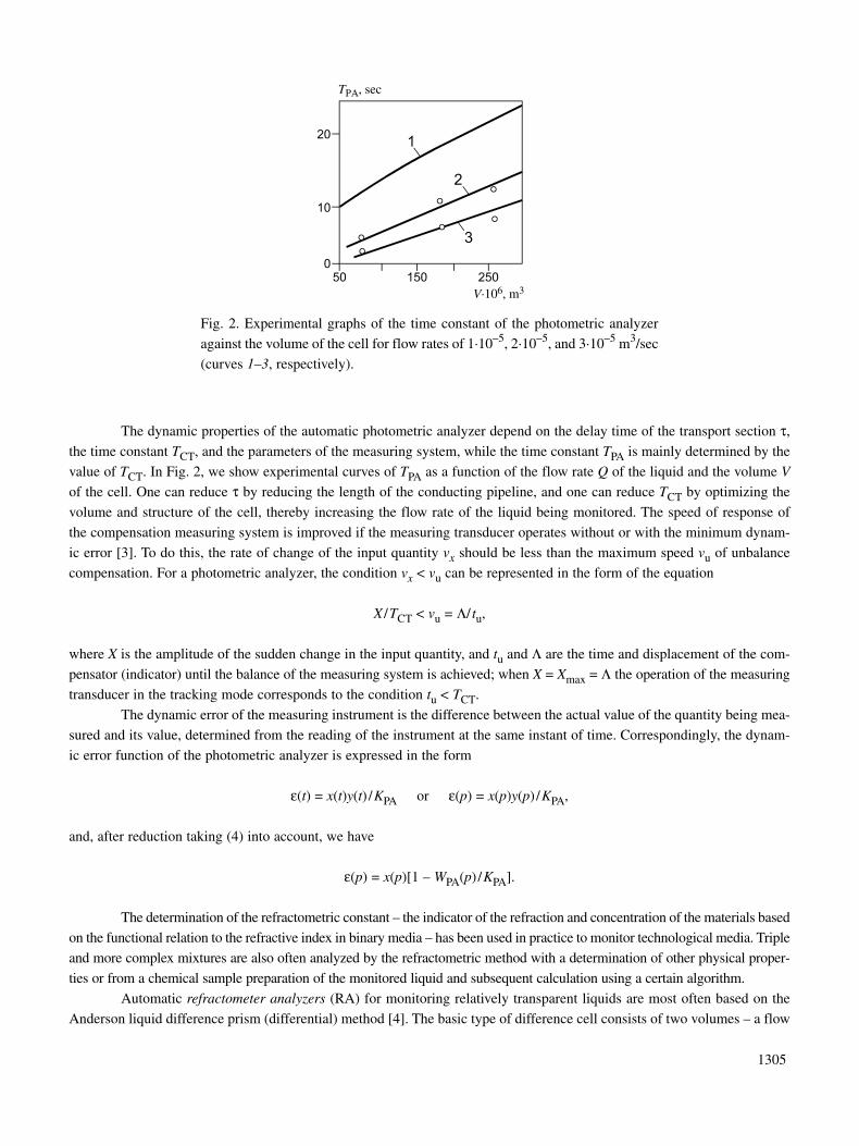
The dynamic properties of the automatic photometric analyzer depend on the delay time of the transport section τ,

the time constant TCT, and the parameters of the measuring system, while the time constant TPA is mainly determined by the

value of TCT. In Fig. 2, we show experimental curves of TPA as a function of the flow rate Q of the liquid and the volume V

of the cell. One can reduce τ by reducing the length of the conducting pipeline, and one can reduce TCT by optimizing the

volume and structure of the cell, thereby increasing the flow rate of the liquid being monitored. The speed of response of

the compensation measuring system is improved if the measuring transducer operates without or with the minimum dynam-

ic error [3]. To do this, the rate of change of the input quantity vx should be less than the maximum speed vu of unbalance

compensation. For a photometric analyzer, the condition vx < vu can be represented in the form of the equation

X /TCT < vu = Λ/ tu,

where X is the amplitude of the sudden change in the input quantity, and tu and Λ are the time and displacement of the com-

pensator (indicator) until the balance of the measuring system is achieved; when X = Xmax = Λ the operation of the measuring

transducer in the tracking mode corresponds to the condition tu < TCT.

The dynamic error of the measuring instrument is the difference between the actual value of the quantity being mea-

sured and its value, determined from the reading of the instrument at the same instant of time. Correspondingly, the dynam-

ic error function of the photometric analyzer is expressed in the form

ε(t) = x(t)y(t) /KPA or ε(p) = x(p)y(p) /KPA,

and, after reduction taking (4) into account, we have

ε(p) = x(p)[1 – WPA(p) /KPA].

The determination of the refractometric constant – the indicator of the refraction and concentration of the materials based

on the functional relation to the refractive index in binary media – has been used in practice to monitor technological media. Triple

and more complex mixtures are also often analyzed by the refractometric method with a determination of other physical proper-

ties or from a chemical sample preparation of the monitored liquid and subsequent calculation using a certain algorithm.

Automatic refractometer analyzers (RA) for monitoring relatively transparent liquids are most often based on the

Anderson liquid difference prism (differential) method [4]. The basic type of difference cell consists of two volumes – a flow

1305

TPA, sec

V·106, m3

Fig. 2. Experimental graphs of the time constant of the photometric analyzer

against the volume of the cell for flow rates of 1·10–5, 2·10–5, and 3·10–5 m3/sec

(curves 1–3, respectively).

volume for the liquid being monitored with refractive index n and a closed volume with a comparison liquid with known

refractive index ncl, placed inside the flowing liquid to equalize the temperatures of the liquids (Fig. 3).

The block diagram of the refractometer analyzer is similar to that shown in Fig. 1 for a photometric analyzer, in which

the compensator C takes the form of a photoreceiver displacement mechanism. Any change in the refractive index n (the concen-

tration) of the liquid being monitored produces a deflection of the beam β, emerging from the cell, proportional to Δn = n – ncl.

Using this relation, the informative parameter of the refractometer analyzer is generated, namely, a change in the angle of deflec-

tion (displacement) of the beam, emerging from the cell, and a static characteristic β = Δn tanγ, where γ is the angle between the

entering beam and the perpendicular to the interface of the flow and closed volumes. Analyzers measure the relative value of the

refractive index and are calibrated in units of refractive index (difference), concentration or arbitrary units.

When the liquid being monitored is at constant temperature, the transfer functions of the cell and the refractometer

analyzer are described by equations similar to (2) and (4), and the latter function has the form

WRA(p) = y(p) /x(p) = KRAe–pτ / [(TCTp + 1)(TMTp + 1)],

where KRA = KCTKMT = y(t) /x(t)t→∞ are the transfer constants of the refractometer analyzer.

Under these temperature conditions, when the measuring transducer is operating in the tracking mode and the input

action x(p) = x0/p, the dynamic error ε(t) and its integral value ε can be defined as

ε = C(τ + TCT).

In refractometer measurements, the main noninformative parameter is the temperature of the liquid being monitored.

The temperature dependence of the refractive index has the following simplified form:

n = n0 + b(θ – θ0),

where n and n0 are the refractive indices at the current temperature θ and the initial temperature θ0, and b is the temperature

gradient of the refractive index of the liquid being monitored.

ετ

ττ( )

;

;( )t

x t

X tt T=

< <

>

⎧⎨⎪

⎩⎪− −

0 0for

e forCT

1306

a b c

Fig. 3. Difference cells with different types of closed volumes: a) placed under the input connecting pipe; b) in the

form of a hollow prism with two refracting surfaces; c) with a sylphon compensator of the liquid pressure.

The temperatures of the monitored and comparison liquids are functionally related as follows: when there is a

change in the temperature of the monitored liquid, its refractive index changes as well as the temperature and refractive index

of the liquid in the closed volume of the cell, and a dynamic error occurs, the value and nature of which depend on the instru-

ment mode of operation and parameters. At a fixed instant of time, the dynamic error can be determined from the function

εθ ≈ b(θ – θcl), where θcl is the temperature of the comparison liquid. Temperature compensation (εθ → 0) is achieved in the

passive heat-exchange mode between the liquids in the flow and closed volumes of the cell and has a dynamic form [5].

The transfer functions of the closed volume of the cell Wclθ(p) and of the flow volume Wf

θ(p) when there is a change

in temperature of the liquid being monitored are expressed as

Wclθ(p) = θcl(p) /θin(p) = Kcl

θ / [(TCTp + 1)(Tclp + 1)];

Wfθ(p) = θout(p) /θin(p) = Kf

θ / (TCTp + 1), Tcl = mCr / (αS),

where θcl, θin, and θout are the temperatures of the liquid in the closed volume at the input and at the output of the flow vol-

ume; Tcl and S are the time constant and area of the walls of the closed volume; m, C, and α are the mass, heat capacity, and

heat transfer coefficient of the comparative liquid; and Kclθ = θcl(t) /θin(t)t→∞, Kf

θ = θout(t) /θin(t)t→∞ are the transfer coeffi-

cients of the closed and flow volumes when there is a change in temperature.

The transfer function of the dynamic error of the cell when there is a change in the temperature of the liquid being

monitored W εCT is defined as the difference in the functions of the flow volume Wf

θ and the closed volume Wclθ:

W εCT(p) = b[Wf

θ(p)Wclθ(p)].

As t → ∞, we have θout(t) = θcl(t) and Kclθ and Kf

θ, and hence

W εCT(p) = K θ

CTbTclp / [(TCTp + 1)(Tclp + 1)].

The transfer function of the error of the refractometer analyzer when there is a change in the temperature of the liq-

uid being monitored is expressed in the form

W εRA(p) = W θ

CT(p)W θMT(p)

or

W εRA(p) = y(p) /x(p) = K θ

RAbTclp / [(TCTp + 1)(TMTp + 1)(Tclp + 1)].

The dynamic error signal when the temperature of the liquid being monitored changes is generated in the same way

as the signal of the informative parameter, and its value can be determined from the deviation of the output signal from the

established value, i.e., εθ(p) = y(p), and correspondingly εθ(p) = W θRA(p)x(p).

1307

t, sec

Fig. 4. Dynamic error of a refractometer analyzer when there is

a change in the temperature of the liquid flowing abruptly (1)

and at a constant speed (2).

When there is a sudden change in the temperature of the liquid being monitored at the input to the cell x(p) = θin /p,

the dynamic error function εθ(t) and its integral value εθ can be found from the equations

εθ(t) = bTclθin{[TCT/(TCT – Tcl)]e–t/TCT + [Tcl/(TCT – Tcl)]e

–t/Tcl]};

εθ = bTclθin.

Graphs of the dynamic error of the refractometer analyzer for a constant and sudden change in the temperature are

shown in Fig. 4. This error can be reduced by optimizing m, Cp, S, and α and reducing Tcl. In view of the difficulties of mak-

ing a theoretical investigation, the value of Tcl was determined experimentally. In the investigation and calculations, we

assumed the conditions Tcl >> TCT, εθ(t) = εθmax, and t = tmax. The time-constant equation then has the form

Tcl = tmax/ ln(bθin /εθmax).

When checking the condition Tcl >> TCT, we established that, when Tcl/TCT = 2–30, the error of the approximation

does not exceed 1 sec. When the temperature of the liquid being monitored changes at a constant rate for an input action of

x(p) = vθ /p2, taking into account the amplitude X, the equation of the time constant takes the form

Tcl = εvθ / (bvθ),

where εvθ is the steady value of the dynamic error, and vθ is the rate of change of the temperature of the liquid being monitored.

The values of εθmax and tmax were determined from the diagram film. Table 1 shows experimental values of the

parameters of different types of cells.

When using a refractometer analyzer with constant construction parameters of the flow and closed volumes, the tem-

perature dynamic error may vary depending on the flow rate of the liquid being monitored, i.e., for different values of the

time constant TCT. In Fig. 5, we show a graph of the maximum value of the dynamic error of a refractometer analyzer against

the ratio TCT/Tcl for a harmonic variation of the temperature of the monitored liquid.

The detailed form of the transfer function of the cell with flow and closed volumes when there is a change in the

temperature of the monitored liquid is as follows:

W θCT = εθ(p) /θ(p) = [kbTclp(Twp + 1)] / [(Twp + 1)(Tclp + 1)(Tθp + 1)] – k1(Tinp + 1)]. (5)

1308

TCT/Tcl

Fig. 5. Graph of the maximum dynamic error of a refractometer

analyzer against the ratio of the time constants of the cell and the

closed volume for a harmonic law of variation of the temperature

θ of the liquid being monitored.

Here

k = Qw/(Qw + αwSw + αclScl); Tcl = mclC / (αclScl);

Tw = mCpw/(αwSw); Tθ = mCp / (Qw + αclScl + αwSw);

k1= (αwSw + αclScl) / (Qw + αwSw + αclScl);

Tin = (αwSwTcl + αclSclTw)/(αclScl + αwSw);

the subscript “w” denotes quantities relating to the walls of the cell.

In Eq. (5), the input quantity is the change in the temperature of the monitored liquid θ(p) from the initial value θ0(θ0 = θcl0 and ε0

θ(p) = 0), and the output quantity is the temperature error εθ(p). For a flow rate of the liquid through the flow

volume Q → ∞, k1 → 0, and k1 → 1. If we assume the flow rate Q is greater and k1 = 0, we can write (5) as

W θCT(p) = bTclp / [(Tθp + 1)(Tclp + 1)]. (6)

In the general case, the temperature error of the instrument will have the form

εθ(p) = {[(bkTcl /a1)(Twp + 1)] / [(p – p1)(p – p2)(p – p3)]}θ(p),

where a1 = TθTclTw, and p1, p2, and p3 are the roots of the characteristic equation.

The solution of the characteristic equation enables us to calculate the coefficients and corrections for (5). They

reflect the effect of the components on the thermal processes in the cell, and they take into account the effect of Tin and the

parameters of the cell walls Tw. Knowing the parameters of the cell, the coefficients and corrections, we can determine Δεθ(p)

in the 10–30 sec interval, when this error reaches a maximum. If the condition [Δεθ(p) /εθmax] << 1 is satisfied for this inter-

val, where εθmax is determined from the temperature error equation with transfer function (6), Eq. (5) enables a sufficiently

accurate result to be obtained. In other cases the transfer function is written as

W θCT(p) = (bkTcl /a1){(Twp + 1)/[(p – p1)(p – p2)(p – p3)]}.

Parameter Value

V, cm3 2 2 2 5 5 5 2 5

S, cm2 20 20 11 28 28 28 11 28

θin, °C 2 3 4 4 5 6 – –

tmax, sec 9 9 10 15 17 20 – –

εθmax, scale division 20 32 17.8 22 17 31.1 – –

bθmax, scale division 30 45.6 22.2 27 34 41 – –

vθ, °C/sec – – – – – – 0.016 0.018

εvθ, scale division – – – – – – 4.45 9

bvθ, scale division/sec – – – – – – 0.09 0.118

Δnmax·10–4 6.6 6.6 18 14.6 14.6 14.6 18 14.6

Tcl, sec 23 26 45 75 78 74 49 76

1309

TABLE 1

In certain situations, the mode of operation where Q → ∞ is impermissible due to constructional and systematic fac-

tors, since an increase in the flow rate may lead to the occurrence of dead zones, deterioration of the mixing, etc. Hence,

the model of the flow cell is limited to the value Qmax. At the same time, for monitoring, for example, viscous polymerizing

plastics or oils, to ensure effective flow it is necessary to increase the flow rate of the liquid. The problem can be solved by

using a refractometer analyzer with a cylindrical cell and internal flow, in which the flow rate of the liquid is unlimited and

there are no stagnation zones. It was established from the results of an investigation of models of refractometer analyzers

under the same conditions that, in the case of an analyzer with a cell having an internal flow, Tcl and, correspondingly, Δεθ(p)

are less than in a refractometer analyzer with a cell with external flow.

The differential equation, representing the functioning of measuring instruments, relates to the complete dynamic

metrological characteristics of measuring instruments, which describe the mathematical model of the dynamic properties.

The dynamics of the automatic analyzers considered (without the transport section) can be represented by a 2nd order linear

differential equation of the form

TCTTMTd2y(t) /dt2 + (TCT + TMT)dy(t) /dt + y(t) = KCTKMTx(t)

and the corresponding equation of the dynamic error

ε(p) = (TCTTMTp + TCT + TMT)pX(p).

REFERENCES

1. GOST 8.009-84, GSI. Standardized Metrological Characteristics of Measuring Instruments.

2. GOST 8.256-77, GSI. Standardization and Determination of the Characteristics of Analog Measuring Instruments.

Basic Definitions.

3. D. D. Kotchenko, Tracking Systems of Automatic Compensators [in Russian], Nedra, Moscow (1965).

4. M. A. Karabegov, “Automatic differential prism refractometers for monitoring technical liquids,” Izmer. Tekhn.,

No. 6, 31–37 (2007); Measur. Techn., 50, No. 6, 619–628 (2007).

5. M. A. Karabegov, L. V. Nalbandov, and S. A. Khurshudyan, “Investigation of automatic optoanalytical instruments

for monitoring the composition of liquids under dynamic operating conditions,” Tr. Metrolog. Inst. SSSR,

No. 193(253), 28–35 (1976).

1310