the dynamics of ultracompact h regionsw.astro.berkeley.edu/~stahler/papers/roth2014.pdf · the...

MNRAS 438, 1335–1354 (2014) doi:10.1093/mnras/stt2278Advance Access publication 2013 December 19

The dynamics of ultracompact H II regions

Nathaniel Roth,1‹ Steven W. Stahler2 and Eric Keto3

1Department of Physics, University of California, Berkeley, CA 94720, USA2Department of Astronomy, University of California, Berkeley, CA 94720, USA3Harvard–Smithsonian Center for Astrophysics, 60 Garden Street, Cambridge, MA 02138, USA

Accepted 2013 November 22. Received 2013 November 18; in original form 2013 October 4

ABSTRACTMany ultracompact H II regions exhibit a cometary morphology in radio continuum emission.In such regions, a young massive star is probably ablating, through its ultraviolet radiation,the molecular cloud clump that spawned it. On one side of the star, the radiation drives anionization front that stalls in dense molecular gas. On the other side, ionized gas streamsoutwards into the more rarefied environment. This wind is underpressured with respect to theneutral gas. The difference in pressure draws in more cloud material, feeding the wind untilthe densest molecular gas is dissipated. Recent, time-dependent simulations of massive starsturning on within molecular gas show the system evolving in a direction similar to that justdescribed. Here, we explore a semi-analytic model in which the wind is axisymmetric andhas already achieved a steady state. Adoption of this simplified picture allows us to study thedependence of both the wind and its bounding ionization front on the stellar luminosity, thepeak molecular density and the displacement of the star from the centre of the clump. Fortypical parameter values, the wind accelerates transonically to a speed of about 15 km s−1, andtransports mass outwards at a rate of 10−4 M� yr−1. Stellar radiation pressure acts to steepenthe density gradient of the wind.

Key words: stars: early-type – stars: formation – ISM: clouds – H II regions – ISM: jets andoutflows.

1 IN T RO D U C T I O N

1.1 Observational background

An ultracompact H II (UCHII) region is one of the earliest signpostsfor the presence of a young, massive star (for reviews, see Church-well 2002 and Hoare et al. 2007). While the star itself is still tooembedded in its parent molecular cloud to be detected optically, itheats up surrounding dust. A small region, some 1017 cm in ex-tent, glows brightly in the far-infrared. Ionization of ambient gasalso creates free–free emission in the radio continuum, with elec-tron densities in excess of 104 cm−3 and thus emission measures of107 pc cm−6 or more. It is through this radio emission, relativelyminor in the overall energy budget, that UCHII regions have beenclassified morphologically.

In their pioneering radio interferometric survey, Wood & Church-well (1989) found that 30 per cent of the spatially resolved regionshave a cometary shape (see also Kurtz, Churchwell & Wood 1994;Walsh et al. 1998). One sees a bright arc of emission filled in byan extended, lower intensity lobe that fades away from the arc. OHmasers may be found along the bright rim. Other UCHII regions

� E-mail: [email protected]

exhibit only the emission arc; presumably, the interior lobe in thesecases is undetectably faint. Still other classes identified by Wood& Churchwell (1989) include: spherical, core-halo (a bright peaksurrounded by a fainter envelope), shell (a ring of emission) andirregular (multiple emission peaks). All told, the cometary mor-phology is the most common one found, and needs to be explainedby any viable theoretical model.

Spectral line studies have been used to probe the kinematicsof these regions. Observations of radio recombination lines (e.g.Afflerbach et al. 1996; Kim & Koo 2001), and infrared fine-structurelines (e.g. Zhu et al. 2005) reveal large line-widths, indicative ofsupersonic flow. In cases where the flow can be spatially resolved,one also sees a velocity gradient. This gradient is steepest in the‘head-to-tail’ direction (Garay, Lizano & Gomez 1994; Garay &Lizano 1999).

Very often, the observed peak in radio continuum or OH maseremission, either of which effectively locates the star, does not co-incide with the peak in molecular lines or submillimetre contin-uum emission, which trace the densest molecular gas and dust (e.g.Mueller et al. 2002; Thompson et al. 2006). This gas is locatedwithin infrared dark clouds, currently believed to be the birth sitesof all massive stars (Beuther et al. 2007). The clumps within theseclouds have typical sizes of 1 pc, number densities of 105 cm−3 andmasses of about 104 M�; some qualify as hot cores (Hofner et al.

C© 2013 The AuthorsPublished by Oxford University Press on behalf of the Royal Astronomical Society

at University of C

alifornia, Berkeley on February 21, 2014

http://mnras.oxfordjournals.org/

Dow

nloaded from

mailto:[email protected]



1336 N. Roth, S. W. Stahler and E. Keto

2000; Hoare et al. 2007). The offset of the peak radio emission ofthe UHCII region from the centre of this clump is typically a fewarcseconds, corresponding to approximately 0.1 pc for a distanceof 1 kpc. Both the cometary morphology and the acceleration ofionized gas are likely related to this physical displacement, as wasfirst emphasized by Kim & Koo (2001).

1.2 Previous models and present motivation

The foregoing observations, taken together, show convincingly thatthe cometary structures represent ionized gas accelerating awayfrom the densest portion of the nearby cloud material. Theoristshave long considered photoevaporating flows created by a massivestar illuminating one face of a cloud (Kahn 1954; Oort & Spitzer1955). The most well-studied classical H II region of all, the Orionnebula, is a prime example of the resulting ‘blister’, here formed bythe massive star θ1 C on the surface of the Orion A molecular cloud(Zuckerman 1973). A tenuous, hemispherical body of ionized gassurrounds θ1 C and the other Trapezium stars, and is flowing awayfrom the background cloud.

When massive stars are still deeply embedded in the densestportion of their parent cloud, it is not obvious how such photoe-vaporating flows can be maintained. Wood & Churchwell (1989)pointed out that the small size of UCHII regions suggests a briefdynamical lifetime. If they undergo pressure-driven expansion at∼10 km s−1, they will expand to a size greater than 0.1 pc in roughly104 yr, or one percent of the lifetime of the host star. In reality, some10 per cent of O stars are associated with UCHII regions, suggestingthat the lifetime of these regions is larger by an order of magnitude.Confinement by thermal pressure alone would result in an emis-sion measure even higher than is observed (Xie et al. 1996). In thecontext of cometary structures, this venerable ‘lifetime problem’raises a fundamental question. What reservoir of matter can feedthe ionized flows over a period of 105 yr?

Hollenbach et al. (1994) suggested that the star may be photoe-vaporating its own accretion disc. When ultraviolet radiation froma massive star impinges on the disc, gas streams off at the soundspeed, at least in that outer region where this speed exceeds the localescape velocity. Lugo, Lizano & Garay (2004) have analysed thislaunching process in more detail. The outer accretion disc radiusof approximately 1015 cm is much smaller than the 1017 cm size ofUCHII regions. Thus, while the model views a disc as the ultimatesource of matter for the ionized flow, it does not address the flow’scometary morphology.

One possibility is that the prominent arc represents the shockinterface between a high-velocity stellar wind and the parent cloud.Massive stars indeed generate, through radiative acceleration, windswith terminal velocities of about 1000 km s−1. If the star itselfmoves through the cloud at supersonic speed, e.g. 20 km s−1, thenthe curved bowshock has the right form (van Buren et al. 1990;Mac Low et al. 1991). Moreover, a star that is moving towardsthe observer creates a ‘core-halo’ structure, also commonly seen.The relatively fast stellar velocity, however, implies that the wholeinteraction would last for a few times 104 yr if the star indeedtravels through a molecular clump 1 pc in size. Consequently, thisbowshock model may fall prey to the lifetime problem. Anotherconcern is that massive stars, with the exception of runaway objects,do not move at such high speeds relative to parent molecular gas.For instance, the Trapezium stars in the Orion nebula cluster havea velocity dispersion of a few km s−1 (Furesz et al. 2008).

Suppose instead that the embedded star is not moving with re-spect to the densest gas, but is displaced from it, as is suggested

by the observations. Then one side of its expanding H II regioneventually erupts into the surrounding low-density medium. Sucha ‘champagne-flow’ model was first explored by Tenorio-Tagle(1979), Bodenheimer, Tenorio-Tagle & Yorke (1979) and Whit-worth (1979) to explain asymmetric, classical H II regions. The highinternal pressure of the H II region accelerates the ionized gas tosupersonic speed away from the ambient cloud, whose density wastaken to be 103 cm−3. Meanwhile, the ionization front steadily ad-vances at several km s−1 into this cloud, generating volumes ofionized gas several parsecs in diameter.

Another model, that of the mass-loaded wind (Dyson 1968),invokes champagne-type dynamics in combination with a stellarwind. The idea is that the wind, perhaps in combination with thestellar radiation field, ablates the cloud, entraining the gas withinit. Pressure gradients may then accelerate the gas in a champagneflow. In some versions of the model, the new mass originates indense globules that are continually being ionized (Lizano et al.1996; Williams, Dyson & Redman 1996; Redman, Williams &Dyson 1998). While successful in explaining the morphologies andlifetimes of UCHII regions, the model does not address in detail howthe dense globules enter the ionized flow. Thus, the mass-loadingprescription adopted was somewhat ad hoc.

Keto (2002a) modelled the growth of an H II region inside aBondi accretion flow. If the ionization front is located inside theBondi radius rB ≡ GM∗/2a2

I , where M∗ is the stellar mass and aI

the ionized sound speed, then gas simply crosses the ionization frontand continues towards the star as an ionized accretion flow. Untilits size reaches rB, the H II region can expand only as the ionizingflux from the star increases along with the stellar mass. The H II

region then exists in steady state, continuously fed by the molecularaccretion. Thus, the lifetime of the H II region is tied to the accretiontime-scale of the star.

Observations of the UCHII region around the cluster of massivestars G10.6−0.4 indicate that this kind of molecular and ionized ac-cretion could be occurring (Keto 2002b). Subsequent observationsof the same cluster (Keto & Wood 2006) also show an asymmetricbipolar outflow of ionized gas. These observations motivated Keto(2007) to develop a model in which inflow and outflow occur si-multaneously in a rotationally flattened geometry. The ionizationcreates an H II region elongated perpendicular to the accretion flow.Where the ionization extends beyond rB, the H II region can ex-pand hydrodynamically as a pressure-driven Parker wind (see alsoMcKee & Tan 2008). Along the equatorial plane, dense moleculargas continues to flow into the H II region. One of the motivationsof this paper is to detail exactly how an ionized outflow may besupplied by inflow of molecular gas, although here we consider amechanism to draw in this gas that is separate from the gravitationalattraction of the star.

Another model combining ionization and gravitational accre-tion was that of Mac Low et al. (2007), who suggested that anUCHII region may form as a gravitationally collapsing substructurewithin a larger, expanding H II region. More detailed simulations byPeters et al. (2010a,b) found that an UCHII region embedded inan accretion flow rapidly changes morphologies through all the ob-served types, and could be sustained by the addition of infallinggas from the parent cloud. The collapsing ionized gas in their sim-ulations creates bipolar molecular outflows, as are observed to ac-company some UCHII regions (Beuther & Shepherd 2005). Peterset al. (2011) also claimed that magnetic pressure might play a sig-nificant role in confining UCHII regions. On the other hand, Arthuret al. (2011) performed their own radiation-magnetohydrodynamicsimulation of an H II region expanding into a turbulent cloud.

at University of C



Dow

nloaded from



The dynamics of ultracompact H II regions 1337

They found that magnetic pressure plays only a minor role inconfinement.

Other recent simulations have combined various elements in theoriginal models to account for the proliferating observational resultsnow becoming available. Henney et al. (2005) simulated a cham-pagne flow in which the ionization front is stalled as it climbs adensity gradient into a neutral cloud supported by turbulent pres-sure. Comeron (1997) explored the coupled roles of champagneflows and stellar winds. Finally, Arthur & Hoare (2006) revised thebowshock idea by introducing a finite but modest stellar velocitywith respect to the cloud.

In this paper, we pursue a different goal. Accepting that everycometary UCHII region is an ionized flow, we elucidate the basicissue of how such a flow may continue to draw in gas from the neutralcloud. We agree with previous researchers that the momentum of theionized flow is not supplied by the star, but by the thermal pressuregradient of the gas itself. A key result of our own study will be todemonstrate that the expansion of this flow causes the ionized gasto become underpressured with respect to the neutral cloud. Thispressure differential draws neutral material from the cloud into thechampagne flow in a self-sustaining manner.

We assume at the outset that the flow is quasi-steady, as wasfound in the late stages of the simulations of Henney et al. (2005)and Arthur & Hoare (2006). This basic simplification allows us torapidly explore parameter space, as we detail below. Thus, we canassess how well our rather minimal set of physical assumptionsexplains the basic characteristics of cometary UCHII regions. Ourquasi-one-dimensional model does not allow us to include evacua-tion by a stellar wind, but we do account for the effect of radiationpressure and show that it is appreciable.

In Section 2 below, we introduce our steady-state model forcometary UCHII regions. Section 3 develops the equations gov-erning the density and velocity of the ionized flow. In Section 4, werecast these equations in non-dimensional form and then outline oursolution strategy. Section 5 presents our numerical results, and Sec-tion 6 compares them to observations. Finally, Section 7 indicatesfruitful directions for future investigations.

2 STEADY-STATE MODEL

2.1 Physical picture

We idealize the molecular cloud as a planar slab, in which the clouddensity peaks at the mid-plane (see Fig. 1). The choice of planar ge-ometry is made for computational convenience and is probably not arealistic representation of the clouds of interest. However, our qual-itative results are not sensitive to the adopted cloud density profile,as we verify explicitly in Section 5 below. We envision a massivestar embedded within this cloud, but offset from the mid-plane, inaccordance with the observations mentioned previously. This off-set creates an asymmetric, ionized region of relatively low density.Towards the cloud mid-plane, this ionized gas resembles a classicalH II region. Its boundary, a D-type ionization front, advances up thedensity gradient. In the opposite direction, the front breaks free andgas streams away supersonically. The pressure gradient within theionized gas creates an accelerating flow away from the cloud. Apartfrom the higher density cloud environment, our model is identicalin spirit to the champagne flows proposed in the past.

Once the velocity of the advancing ionization front falls signif-icantly below the ionized sound speed, the flow becomes steady-state. We adopt this steady-state assumption in our model, and as-sume that the structure of the background cloud is evolving over a

Figure 1. Our flow schematic. A massive star is situated to one side of aninitially neutral cloud. It creates, as in the original champagne model, anasymmetric H II region of relatively low density. Towards the mid-plane, theionization front is stalled by rising cloud density. In the opposite direction,the front has broken free. The high pressure of ionized gas creates an ac-celerating flow away from the densest gas. At the base of the ionized flow,the pressure has been relieved sufficiently such that the neutral cloud gas isslightly overpressured with respect to the ionized gas.

long time-scale compared to the ionized sound crossing time. In thesimulations of Arthur & Hoare (2006), a steady flow is approachedsome 105 yr after the massive star turns on. By this point, the ion-ization front has virtually come to rest in the frame of the star. Wewill later determine more precisely the speed of the ionization frontin our model and show that it is consistent with the steady-state as-sumption. The shock that originally formed ahead of the ionizationfront, as it transitioned from R-type to D-type, has by now advanceddeep into the cloud and died away.

The H II region facing the cloud mid-plane expands, albeit slowly.While the ionized gas is optically thick to ultraviolet radiation fromthe star, some does leak through and strikes the cavity wall withinthe neutral cloud. Additional gas is thus dissociated and ionized, andstreams off the wall to join the outward flow. While the injectionspeed at the wall is subsonic, the thermal pressure gradient withinthe ionized gas accelerates it to supersonic velocity. Both this flowand the advancing front erode the cloud, whose structure graduallyevolves in response.

2.2 Tracing the ionization front

We will always consider systems that possess azimuthal symmetry.We establish a spherical coordinate system whose origin is at thestar. The polar direction, θ = 0, coincides with the central axisof the flow depicted in Fig. 1. Let N ∗ denote the total numberof ionizing photons per time generated by the star. If we furtherassume ionization balance within the volume of the ionized cavity,and make use of the on-the-spot approximation, then the ionizingradiation extends out to the cavity wall rf(θ ), given implicitly by

N∗4 π

= αB

∫ rf

0dr r2 [nI(r, θ )/2]2 + r2

f F∗ , wall(θ ) . (1)

Here, αB is the case B recombination coefficient (Osterbrock 1989,chapter 2). We have pulled this factor out of the integral since itdepends only on the ionized gas temperature, which we assume tobe spatially uniform. The term nI is the number density of ionizedgas, including both protons and electrons. For simplicity, we haveassumed that the composition of the gas is pure hydrogen, so thenumber of free protons is equal to the number of free electrons andboth of these number densities are equal to nI/2. Finally, F∗ , wall(θ )is that portion of the star’s ionizing photon flux which escapes the

at University of C



Dow

nloaded from




H II region and strikes the wall of the cavity. This remnant flux iscritical for maintaining the flow.

But how important is the second term of equation (1) in a quan-titative sense? Each photon striking the front ionizes a hydrogenatom, itself already dissociated from a hydrogen molecule, therebycreating a proton and an electron. Let f be the number flux of pro-tons and electrons injected into the flow at each position along thefront. Thus, F∗ , wall = f/2 at each angle θ , and we may write theforegoing equation as

N∗4 π

= αB

∫ rf

0dr r2 (nI/2)2 + r2

f f

2. (2)

The flux f is of the order of nI aI, where nI is now a typical value ofthe ionized gas number density. If rf in equation (2) now representsthe size scale of the flow, then the ratio of the second to the firstright-hand term in this equation is of the order of

aI

αB nI rf∼

(aI

acl

)3acl

αB ncl rf, (3)

where acl and ncl are the effective sound speed and number densitywithin the cloud (see below). Here, we have assumed that the ionizedmaterial is at least in rough pressure balance with the cloud, so thatnI a

2I ≈ ncl a

2cl. For the dense clumps that harbour young massive

stars, ncl ∼ 105 cm−3 and acl ∼ 2 km s−1 (Garay & Lizano 1999).Further using rf ∼ 1017 cm, aI ∼ 10 km s−1 and αB ∼ 10−13 cm3 s−1,we find that the ratio of terms is of the order of 10−2. In practice,therefore, we neglect the second term entirely.1 We trace the ion-ization front by finding that function rf(θ ) which obeys the approx-imate, but quantitatively accurate relation,

N∗4 π

= αB

∫ rf

0dr r2 (nI/2)2 . (4)

2.3 Cloud density and gravitational potential

Even within our simplifying assumption of axisymmetry, it wouldbe a daunting task to trace a fully two-dimensional flow. Whilewe accurately follow the ionization front bounding the flow in twodimensions, we further assume that the density and velocity areonly functions of z. In this quasi-one-dimensional model, we areeffectively averaging the ionized density nI and velocity u laterallyat each z-value. This simplification is innocuous in regions wherethe lateral change in these quantities is relatively small. It is moreproblematic when the ionized gas becomes overpressured with re-spect to the ambient cloud. Luckily, most of the radio emissioncomes from the densest portion of the flow, well before this pointis reached. Hence, our model produces reasonably accurate resultswhen predicting observed emission measures.

Turning to the cloud itself, we assume it to be self-gravitating,with an internal supporting pressure arising from turbulence. Hence,we do not consider the possibility that the object is in a state of col-lapse. We crudely model the turbulence by adopting an isothermalequation of state, characterized by an effective sound speed acl. Inour model, it is only the mass of the cloud that affects the flow grav-itationally. That is, we neglect both the self-gravity of the ionizedgas, and the pull of the massive star. The latter force is negligible

1 In the terminology of Henney (2001), our photoevaporation flow is recom-bination dominated. If the second right-hand term in equation (2) wererelatively large, the flow would be advection dominated. According toHenney (2001), knots in planetary nebulae fall into this category.

outside the Bondi radius RB ≡ G M∗/2 a2I , where M∗ is the stellar

mass. For representative values M∗ = 20 M� and aI = 10 km s−1,RB = 90 au, much less than the size of UCHII regions.

Our cloud is an isothermal self-gravitating slab whose mid-planeis located at z = −H∗ (see Fig. 1). Solving the equations of hydro-static equilibrium along with Poisson’s equation yields the neutralcloud density ncl and the gravitational potential �cl

ncl = n0 sech2

(z + H∗

Hcl

), (5)

�cl = −a2cl ln sech2

(z + H∗

Hcl

). (6)

Here, n0 is the mid-plane number density of hydrogen molecules,each of mass 2 mH and Hcl is the scale thickness of the slab:

Hcl ≡[

a2cl

2 π G (2 n0 mH)

]1/2

. (7)

A representative value for n0 is 105 cm−3. Combining this with aturbulent velocity dispersion of acl = 2 km s−1 yields a Jeans massof the order of 102 M�, far less than the 104 M� clumps in giantmolecular clouds spawning massive stars and their surroundingclusters. We stress again that our cloud is a relatively small fragmentcontaining the newborn star. In our view, it is the high density ofthis gas that determines the morphology of the UCHII region, andthe dispersal of the clump that sets the characteristic lifetime.

2.4 Radiation pressure

Quantitative modelling of H II regions, and UCHII regions in par-ticular, has generally neglected the dynamical effect of radiationpressure from the massive star (see, however, Krumholz & Matzner2009). For the very dense environments we are now considering,the radiative force has substantial influence on the ionized flow, aswe shall demonstrate through explicit calculation.

Suppose the star emits photons with mean energy ε. Those travel-ling in the direction θ with respect to the central axis carry momen-tum (ε/c)cos θ in the z-direction. If we assume that the gas is in ion-ization equilibrium, then the number of photons absorbed per unitvolume of gas equals the corresponding volumetric rate of recombi-nation, (nI/2)2αB. The assumption of ionization equilibrium is justi-fied because the typical recombination time, trec ∼ (nIαB)−1 ∼ 108 s,is much less than the flow time tflow ∼ rf/aI ∼ 1011 s.

The radiative force per volume is the product of the pho-ton momentum and the volumetric rate of ionization, or(ε/c)cos θ (nI/2)2αB. To obtain frad, the radiative force per unitmass of gas, we divide this expression by the ionized mass den-sity, mHnI/2. We thus find

frad = ε 〈cos θ〉 nI αB

2 mHc. (8)

This expression is consistent with that given in Krumholz & Matzner(2009, section 2) if we add the condition of ionization balance. Note,finally, that ε in equation (8) is implicitly a function of N∗, a factthat we shall use later.

In accordance with our quasi-one-dimensional treatment, we havelaterally averaged cos θ at fixed z. Explicitly, this average, weightedby the cross-sectional area is

〈cos θ〉 = 2 ηz2

R2

⎛⎝

√1 + R2

z2− 1

⎞⎠ . (9)

at University of C



Dow

nloaded from




Here, R(z) is the cylindrical radius from the central axis to theionization front at each z, and η = +1 or −1 for positive andnegative z, respectively. At z = 0, the level of the star, we set〈cos θ〉 = 0. At the base of the flow, 〈cos θ〉 = −1. We define thedistance from this point to the star as Hb ≡ rf (π), and show it inFig. 1.

3 FLOW EQUATIO N S

3.1 Mass and momentum conservation

To obtain laterally averaged dynamical equations, consider a con-trol volume of height �z spanning the flow, as pictured in Fig. 2.This volume has cylindrical radius R and R + �R at its lower andupper surfaces, respectively. Let uI(z) be the average flow speedin the z-direction. Similarly, let ninj and vinj represent the numberdensity and speed, respectively, of ionized gas being injected intothe flow just inside the ionization front. Then, the requirement ofmass conservation is

d

dt(π R2 �z nI) = π R2 nI uI − π(R + �R)2(nI + �nI)(uI + �uI)

+ 2 π R√

�R2 + �z2 ninj vinj . (10)

Here, the first two terms of the right-hand side are the rate of massadvection through the bottom and top layers of the control volume,respectively. The final right-hand term is the rate of mass injection.We assume that the injected flow direction is normal to the ionizationfront. Henceforth, we will drop the subscript I when referring to thedensity and velocity of the ionized flow.

Under our steady-state assumption, the left-hand side of equation(10) vanishes. Dividing through by �z, and taking the limit �z → 0,leads to

d

dz(R2 n u) = 2 R

√1 +

(dR

dz

)2

ninj vinj . (11)

We will later derive an expression for vinj from the jump conditionsacross the ionization front and show that this velocity is subsonic,i.e. vinj < aI at any z. Although our derived vinj is properly measuredin the rest frame of the ionization front, we will show in Section 3.2that the front is moving very slowly compared to aI. Thus, vinj isalso, to a high degree of accuracy, the speed of the injected gas inthe rest frame of the star.

Figure 2. Control volume diagram for a segment of the ionized flow. Thetrapezoidal section displayed here, represents a meridional slice of the ion-ized flow – one should imagine rotating this diagram about the centralvertical symmetry axis in order to generate the represented volume.

Another crucial assumption we will make is that ninj = n, i.e.the injected density is the same as the laterally averaged flow valueat any height. This condition seems to hold at least approximatelyin the simulations of Arthur & Hoare (2006), and is physicallyplausible when one considers that lateral density gradients will tendto be smoothed out if the velocity components in that direction aresubsonic. After making this assumption, we are left with

d

dz(R2 n u) = 2 R

√1 +

(dR

dz

)2

n vinj . (12)

Requiring conservation of z-momentum for the control volumeleads to

d

dt(π R2 �z n u) = π R2 n u2 − π(R + �R)2(n + �n)(u + �u)2

+ 2 π R n v2inj �R + π R2 n aI

2 − π (R + �R)2(n + �n)aI2

+ 2 π R �R2 + �z2 n aI2�R − π R2 �z n

d�cl

dz

+ π R2 �z n frad, (13)

where �cl is the gravitational potential from equation (6) and frad isthe radiative force per mass from equation (8). Included are termsrepresenting both static pressure and the advection of momentumthrough the top, bottom and sides of the control volume. For theadvective terms, we have again replaced ninj by n. The geometricfactor

√1 + (dR/dz)2 present in equation (12) disappears because

its inverse is used when projecting the injected momentum into thez-direction. We apply the steady-state condition and divide equation(13) through by πR2 n �z. After taking the �z → 0 limit andcombining with equation (12), we obtain

udu

dz= −a2

I

n

dn

dz− d�cl

dz+ frad + 2

R

dR

dzv2

inj

− 2

R

√1 +

(dR

dz

)2

vinj u . (14)

This equation resembles the standard Euler momentum equation inone dimension, but has two additional terms. The first accounts forinjection of z-momentum via ram pressure. The second representsthe inertial effect of mass loading.

3.2 Jump conditions across the ionization front

In the rest frame of the ionization front, upstream molecular gasapproaches at speed v′

cl and leaves downstream as ionized gas,at speed v′

inj. We assume that the intermediate photodissociationregion, consisting of neutral hydrogen atoms, is geometrically thin.2

Conservation of mass and momentum across the ionization front isexpressed in the jump conditions

(1/2) n v′inj = 2 ncl v

′cl (15a)

(1/2) n(a2

I + v′inj

2)

= 2 ncl

(a2

cl + v′cl

2)

. (15b)

The factors of 1/2 and 2 in both equations account for the factthat each hydrogen molecule has a mass of 2 mH, while each particle

2 Roshi et al. (2005, section 4.2) estimate the PDR thickness in G35.20−1.74to be of the order of 10−4 pc.

at University of C



Dow

nloaded from




of ionized gas has a mean mass of mH/2. We solve equation (15a)for v′

cl:

v′cl = 1

4

n

nclv′

inj , (16)

and use this result in equation (15b) to derive an expression for v′inj:

v′inj = aI

√16n2

cl/β − 4n ncl

4n ncl − n2, (17)

where β ≡ a2I /a

2cl � 1. As long as the ionized gas is underpres-

sured with respect to the neutral molecular gas, β n < 4 ncl, and thequantity inside the square root in equation (17) is positive, guaran-teeing a solution for v′

inj. Using this inequality, equation (16) tellsus that v′

cl < v′inj/β . In all our solutions, v′

inj is subsonic. Thus, theionization front moves relatively slowly into the cloud, and we mayset the lab frame injection velocity vinj equal to v′

inj. Since we knowncl at all z, equation (17) gives us vinj as a function of z and n, whichwe may use in the mass and momentum equations (12) and (14).

3.3 Decoupled equations of motion

The mass and momentum conservation equations can be combinedto solve separately for the derivatives of the velocity and density.These decoupled equations are

du

dz=

(1

a2I − u2

) ⎡⎣ − 2 u

1

R

dR

dz

(a2

I + v2inj

)

+ 2 vinj1

R

√1 +

(dR

dz

)2 (a2

I + u2) + u

d�cl

dz− u frad

⎤⎦(18)

dn

dz=

(1

a2I − u2

) ⎡⎣2 n

1

R

dR

dz

(u2 + v2

inj

)

− 4 n1

R

√1 +

(dR

dz

)2

u vinj − nd�cl

dz+ n frad

⎤⎦ . (19)

The right-hand sides of both equations have denominators thatvanish when u = aI. Thus, we must take special care when inte-grating through the sonic point, as is also true in steady-state windsand accretion flows of an isothermal gas. If we were to ignore theterms relating to mass injection, radiation pressure and self-gravity,then the sonic transition would occur when dR/dz = 0, as in ade Laval nozzle. In our case, the extra terms cause the sonic transi-tion to occur at other locations.

4 N O N - D I M E N S I O NA L I Z AT I O N A N DS O L U T I O N S T R AT E G Y

4.1 Characteristic scales

A representative ionizing photon emission rate is 1049 s−1, whichcorresponds to an O7.5 star (Vacca, Garmany & Shull 1996). Wedenote this emission rate by N49. We define a non-dimensionalemission rate normalized to that value:

N∗ = N∗N49

. (20)

To find characteristic density- and length-scales for the flow,consider first Hcl, the scaleheight of the neutral cloud. According to

equation (7), this quantity depends on both the effective sound speedacl, which we fix at 2 km s−1, and on the mid-plane cloud density n0,which will be a free parameter. A second length of importance is theStromgren radius of fully ionized gas of uniform particle numberdensity n, given by

RS ≡(

3N∗4παB(n/2)2

)1/3

. (21)

Note the appearance of n/2 in our expression. This is the num-ber density of either protons or electrons, the species that actuallyrecombine.

For a cometary flow to exist at all, it must be true that RS ∼ Hcl.If RS Hcl, the H II region would be trapped within the cloud andunable to generate the observed flow. If, on the other hand, RS � Hcl,the ionized region would be free to expand in all directions, againcontrary to observation. For the purpose of defining a characteristicionized density-scale, we first set N∗ = N49 in equation (21). Wethen set n0 = βn/4 in equation (5), and solve for the ionized densityn that satisfies the relation Hcl = RS. We label this density n49, andfind that it can be expressed as

n49 = 9π β3

(G mH

a2cl

)3 (N49

αB

)2

= 1.4 × 104 cm−3 . (22)

We insert this value of n49 into equation (21) and set the resulting RS

equal to the characteristic length-scale Z49. We find for this length

Z49 = 1

3π β2

(G mH

a2cl

)−2 (N49

αB

)−1

= 0.18 pc . (23)

It is encouraging that our values for n49 and Z49 match typicalobservations for UCHII regions (Churchwell 2002).

4.2 Non-dimensional equations

We first normalize all lengths by Z49:

r ≡ r/Z49 (24a)

z ≡ z/Z49 , (24b)

and all densities by n49:

n0 ≡ n0/n49 (25a)

n ≡ n/n49 . (25b)

Since the ionized flow is transonic, we normalize all velocities tothe ionized sound speed aI, which we fix at 10 km s−1:

u = u/aI . (26)

We introduce a non-dimensional expression for the force permass due to radiation pressure:

frad ≡ frad

(a2

I

Z49

)−1

. (27)

This non-dimensional quantity is the radiative force relative to thatfrom thermal pressure. Then, using equation (8) for frad, we have

frad = 〈cos θ〉(

ε/c

mH aI

) {Z49/aI

[(n/2) αB]−1

}. (28)

The second factor on the right is the ratio of the momentum ofan ionizing photon to the thermal momentum of a gas particle.

at University of C



Dow

nloaded from




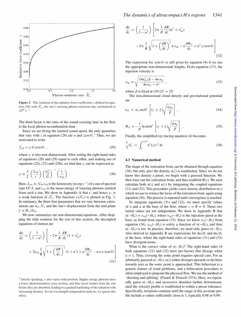
Figure 3. The variation of the radiative force coefficient γ defined in equa-tion (30) with N∗, the star’s ionizing photon emission rate, normalized to1049 s−1.

The third factor is the ratio of the sound crossing time in the flowto the local photon recombination time.

Since we are fixing the ionized sound speed, the only quantitiesthat vary with z in equation (28) are n and 〈cos θ〉.3 Thus, we aremotivated to write

frad = γ n 〈cos θ〉 , (29)

where γ is also non-dimensional. After setting the right-hand sidesof equations (28) and (29) equal to each other, and making use ofequations (22), (23) and (25b), we find that γ can be expressed as

γ ≡ 3

2

(L49

c

) (a4

cl

G

)−1 (ε

ε49

). (30)

Here, L49 ≡ N49 ε49 is the luminosity (in erg s−1) of a star of spectraltype O7.5, and ε49 is the mean energy of ionizing photons emittedfrom such a star. We show in Appendix A that ε, and hence γ , isa weak function of N∗. The function γ (N∗) is plotted in Fig. 3.In summary, the three free parameters that we vary between calcu-lations are n0, N∗ and the star’s displacement from the mid-planeζ ≡ H∗/Z49.

We now summarize our non-dimensional equations. After drop-ping the tilde notation for the rest of this section, the decoupledequations of motion are

du

dz=

(1

1 − u2

) ⎡⎣ − 2 u

1

R

dR

dz(1 + v2

inj)

+ 2vinj1

R

√1 +

(dR

dz

)2

(1 + u2) + ud�cl

dz− u n γ 〈cos θ〉

⎤⎦

(31)

3 Strictly speaking, ε also varies with position. Higher energy photons havea lower photoionization cross-section, and thus travel farther from the starbefore they are absorbed, leading to a gradual hardening of the radiation withincreasing distance. In our wavelength-independent analysis, we ignore thiseffect.

dn

dz=

(1

1 − u2

) ⎡⎣2 n

1

R

dR

dz(u2 + v2

inj)

− 4 n1

R

√1 +

(dR

dz

)2

u vinj − nd�cl

dz+ n2 γ 〈cos θ〉

⎤⎦.

(32)

The expression for 〈cos θ〉 is still given by equation (9) if we usethe appropriate non-dimensional lengths. From equation (17), theinjection velocity is

vinj =√

16n2cl/β − 4n ncl

4n ncl − n2, (33)

where β is fixed at (10/2)2 = 25.The non-dimensional cloud density and gravitational potential

are

ncl = n0 sech2

[(z + ζ )

√4 n0

β

], (34)

�cl = − 1

βln sech2

[(z + ζ )

√4 n0

β

]. (35)

Finally, the simplified ray tracing equation (4) becomes

1

3N∗ =

∫ rf (θ )

0n2(z) r2 dr . (36)

4.3 Numerical method

The shape of the ionization front can be obtained through equation(36), but only after the density n(z) is established. Since we do notknow this density a priori, we begin with a guessed function. Wethen trace out the ionization front, and thus establish R(z). We nextcalculate both n(z) and u(z) by integrating the coupled equations(31) and (32). This procedure yields a new density distribution n(z)which we use to retrace the locus of the ionization front, again usingequation (36). The process is repeated until convergence is reached.

To integrate equations (31) and (32), we must specify valuesof n and u at the base of the flow, where z = R = 0. These twoinitial values are not independent. We show in Appendix B thatu(−Hb) = vinj(−Hb), where vinj(−Hb) is the injection speed at thebase, as found from equation (33). Since we know ncl(−Hb) fromequation (34), vinj(−Hb) is solely a function of n(−Hb), and thusu(−Hb) is too. In practice, therefore, we need only guess n(−Hb).Also derived in Appendix B are expressions for du/dz and dn/dz

at the base, where the right-hand sides of equations (31) and (32)have divergent terms.

What is the correct value of n(−Hb)? The right-hand sides ofboth equations (31) and (32) have pre-factors that diverge whenu = 1. Thus, crossing the sonic point requires special care. For anarbitrarily guessed n(−Hb), u(z) either diverges upwards or declinestowards zero as the sonic point is approached. This behaviour is ageneric feature of wind problems, and a bifurcation procedure isoften employed to pinpoint the physical flow. We use the method of‘shooting and splitting’ (Firnett & Troesch 1974). Here, we repeat-edly guess n(−Hb), and successive densities farther downstream,until the velocity profile is established to within a preset tolerance.Specifically, iterations continue until the range of this accurate pro-file include u-values sufficiently close to 1, typically 0.98 or 0.99.

at University of C



Dow

nloaded from




To jump over the sonic point, we use the current values of du/dz

and dn/dz to perform a single first-order Euler integration step,typically with a z-increment of 0.01–0.03, depending on the valuesof the derivatives. Once we are downstream from the sonic point,we revert to direct integration of equations (31) and (32).

A key feature of the flows we generate is that the density nearthe base is low enough that the ionized gas is underpressured withrespect to the neutral cloud. The pressure drop causes neutral gasto be drawn into the flow and thereby replenish it. Driven by acombination of thermal and radiative forces, the flow accelerates.Thus, its density falls, but the decline is mitigated by the continualinflux of fresh gas. On the other hand, the cloud density alwaysfalls sharply (see equation 34). Eventually, ncl(z) reaches the valueβn(z)/4, at which point the ionized and neutral gas have equalpressures. According to equation (33), no more neutral gas is drawninto the flow beyond this point. In reality, the flow diverges laterallyand its density also falls steeply. We do not follow this spreadingprocess, but end each calculation at the point where the pressurescross over.

5 R ESULTS

5.1 Fiducial model characteristics

For our fiducial model, we set the three non-dimensional parame-ters to: n0 = β/4; N∗ = ζ = 1. The value of n0 is chosen so thatthe cloud mid-plane is in pressure balance when the flow density n

is unity. Dimensionally, the mid-plane density is 8.8 × 104 cm−3,the star’s photon emission rate is N∗ = 1 × 1049 s−1, and the staris displaced from the mid-plane by H∗ = 0.18 pc. Fig. 4 shows theconverged shape of the ionization front for this case. The rapid flar-ing of the base essentially reproduces the typical cometary shapesobserved. Of course, a more precise comparison is between the pre-dicted and observed emission measures. Here, too, the qualitativeagreement is good, as we will later demonstrate.

The lowest dashed line in Fig. 4 represents the cloud mid-plane.Note that the base of the ionization front lies slightly below it. Wehave also displayed, as the middle dashed line, the sonic transition.In this particular model, the flow speed reaches aI close to thez-position of the star. This near match does not hold throughoutmost of parameter space. For example, lowering the stellar emissionrate N∗ moves the sonic transition farther above the star. Finally, theuppermost dashed line marks the height where the internal pressure

Figure 4. Converged ionization front shape for our fiducial UCHII region,with the star’s position indicated. In this and succeeding figures, all physicalvariables are displayed non-dimensionally. The lowest dashed line representsthe z-position of the cloud mid-plane. The middle dashed line represents thez-position of the sonic point. Finally, the upper dashed line is the endpoint ofour solution, where the pressures of the ionized and neutral gas cross over.

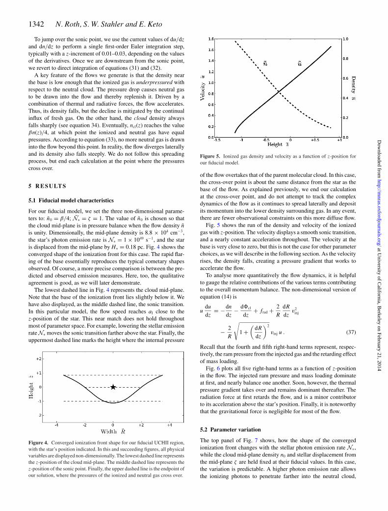
Figure 5. Ionized gas density and velocity as a function of z-position forour fiducial model.

of the flow overtakes that of the parent molecular cloud. In this case,the cross-over point is about the same distance from the star as thebase of the flow. As explained previously, we end our calculationat the cross-over point, and do not attempt to track the complexdynamics of the flow as it continues to spread laterally and depositits momentum into the lower density surrounding gas. In any event,there are fewer observational constraints on this more diffuse flow.

Fig. 5 shows the run of the density and velocity of the ionizedgas with z-position. The velocity displays a smooth sonic transition,and a nearly constant acceleration throughout. The velocity at thebase is very close to zero, but this is not the case for other parameterchoices, as we will describe in the following section. As the velocityrises, the density falls, creating a pressure gradient that works toaccelerate the flow.

To analyse more quantitatively the flow dynamics, it is helpfulto gauge the relative contributions of the various terms contributingto the overall momentum balance. The non-dimensional version ofequation (14) is

udu

dz= −dn

dz− d�cl

dz+ frad + 2

R

dR

dzv2

inj

− 2

R

√1 +

(dR

dz

)2

vinj u . (37)

Recall that the fourth and fifth right-hand terms represent, respec-tively, the ram pressure from the injected gas and the retarding effectof mass loading.

Fig. 6 plots all five right-hand terms as a function of z-positionin the flow. The injected ram pressure and mass loading dominateat first, and nearly balance one another. Soon, however, the thermalpressure gradient takes over and remains dominant thereafter. Theradiation force at first retards the flow, and is a minor contributorto its acceleration above the star’s position. Finally, it is noteworthythat the gravitational force is negligible for most of the flow.

5.2 Parameter variation

The top panel of Fig. 7 shows, how the shape of the convergedionization front changes with the stellar photon emission rate N∗,while the cloud mid-plane density n0 and stellar displacement fromthe mid-plane ζ are held fixed at their fiducial values. In this case,the variation is predictable. A higher photon emission rate allowsthe ionizing photons to penetrate farther into the neutral cloud,

at University of C



Dow

nloaded from




Figure 6. The magnitude of each of the terms in the momentum equation (37) as a function of z-position. The thermal pressure gradient, along with the rampressure from injection of ionized gas, act to accelerate the flow, while mass loading and the gravity of the parent cloud decelerate it. Radiation pressure mostlyacts to decelerate the flow, but for z > 0 it makes a small contribution towards accelerating it.

Figure 7. Effect of parameter variation on the shape of the ionization front. Within each panel, the star is located at (0,0). In this and subsequent graphs, thefiducial model is indicated by a solid black line. For the entire study, β is set to 25.

in a manner similar to how the Stromgren radius of a spherical H II

region increases with emission rate. A larger luminosity also leadsto more flaring of the ionization front at large values of z.

We did not consider systems with photon emission rateN∗ < 0.1 because, at those low luminosities, the fraction of thestar’s luminosity that is composed of ionizing photons drops rapidly.We also found that, given our fiducial values of n0 and ζ , we couldnot achieve transonic solutions with N∗ � 1. As can be seen fromthe plot of velocity, u is already quite close to 0 forN∗ = 1. Attempt-ing to raise the photon emission rate any higher without changing

the other parameters creates such a large ionized density near thebase that the flow is no longer underpressured with respect to thecloud. It is possible to create flows with higher values of N∗ if, forexample, ζ is increased at the same time.

Generally, we find that the density profile of the ionized flowmimics that of the neutral cloud. Fig. 8 shows how the density andvelocity profiles vary when the stellar luminosity is changed. Theflow structure remains strikingly similar as the luminosity is varied,changing primarily in spatial extent, because a higher luminosityallows ionizing radiation to penetrate farther into the cloud. The fact

at University of C



Dow

nloaded from




Figure 8. Density and velocity profiles for various ionizing photon emission rates. The stellar displacement ζ and the mid-plane cloud density n0 are heldfixed at their fiducial values of 1 and β/4, respectively.

that the density and velocity profiles do not show other significantvariations with luminosity reinforces the conclusion that it is thedensity structure of the neutral cloud that sets the spatial variationin the ionized flow.

The second panel of Fig. 7 shows how the shape of the convergedionization front changes with the stellar displacement ζ . Here, theeffect is similar to that of increasing N∗. With higher ζ , the ioniz-ing photons penetrate a larger distance into the cloud, in this casebecause they encounter a lower density when the star is displacedfarther from the cloud mid-plane. Note also the flaring at large z,which increases sharply for higher ζ .

Fig. 9 shows how the density and velocity profiles vary when ζ

is changed. Again, the ionized gas density tracks that of the neutralcloud. For larger offsets, the flow begins in a less dense portion ofthe cloud, and the density of the ionized flow is smaller. Since theionizing stellar photons penetrate farther into the cloud when ζ islarger, the flow begins at more negative values of z. The velocityprofiles shift along the z-axis as ζ is varied, but the accelerationremains roughly the same.

Attempting to lower ζ below a value of unity, while keeping n0

and N∗ fixed at their fiducial values, results in the same problem asattempting to increase N∗ on its own. Solutions with lower valuesof ζ can be achieved only if n0 is simultaneously increased or N∗is decreased. Increasing ζ alone also leads to a large amount offlaring of the ionization front. For ζ = 2, the flaring at the locationof pressure cross-over is such that R/Hb = 5.3. As we shall see inSection 6.1, this aspect ratio is large compared to observations.

The third panel of Fig. 7 shows how the shape of the ionizationfront changes when n0 is varied on its own. In this case, the variationis more complex. As can be seen from equations (5) and (7), chang-ing n0 changes not only the overall magnitude of the density profile,but also the steepness of its falloff. When n0 is increased from β/4to β/2, the rise in the mid-plane density means that radiation cannotpenetrate as far, and the base of the ionized flow moves closer to thestar. However, as n0 is increased further to 3β/4, the steeper falloff

of the density comes into play, and the distance between the starand the base of the flow remains nearly constant.

We may effectively factor out the increasing cloud scaleheight if,instead of increasing n0 on its own, we simultaneously decrease ζ

so that H∗/Hcl remains equal to unity. This result of this exercise isshown in the bottom panel of Fig. 7. As n0 increases and ζ decreases,the shape of the flow remains strikingly similar, changing primarilyin spatial extent. In all cases, Hb/Hcl remains close to unity, rangingfrom 1.21 when n0 = β/6 to 0.94 when n0 = 3β/4.

Fig. 10 shows how the density and velocity profiles respond tochanges in n0. For a denser neutral cloud, the ionized flow alsobegins at a larger density. At the same time, the density of boththe neutral and ionized gas drops more rapidly for a larger n0, andthe z-extent of the flow diminishes. Finally, since the ionized gasis primarily accelerated via pressure gradients, a steeper decline indensity also corresponds to a more rapid acceleration.

We may again factor out the effect of scaleheight by varyingn0 and ζ simultaneously in the manner described previously. Theresulting density and velocity profiles are shown in Fig. 11. In thiscase, the density at the base of the ionized flow again increases withrising n0, but now in a more systematic manner. In fact, this basedensity remains almost exactly equal to 4n0/β, reflecting the factthat the flows are beginning at pressures very close to the neutralcloud pressure. This near-pressure equality also accounts for the factthat the velocities begin near zero in all of these flows. The velocityprofiles are remarkable for the fact that they share an anchor pointnear the stellar position at z = 0. Their z-length-scales correlatetightly with the changing cloud scaleheight.

5.3 Mass, momentum and energy transport

We next consider the total rate at which the neutral cloud adds massto the ionized flow. Dimensionally, this rate, from the base to any

at University of C



Dow

nloaded from




Figure 9. Density and velocity profiles for various values of the stellar displacement ζ . The photon emission rate N∗ and the mid-plane density n0 are heldfixed at their fiducial values of 1 and β/4, respectively.

Figure 10. Density and velocity profiles for various mid-plane densities of the neutral cloud, n0. The non-dimensional ionizing photon emission rate N∗ andstellar offset from the mid-plane ζ are held fixed at their fiducial values of 1.

height z, is

M(z) ≡ 2π

∫ z

−Hb

ρ vinj R

√1 +

(dR

dz

)2

dz . (38)

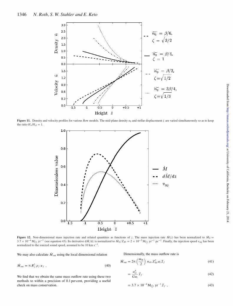
Fig. 12 displays M(z) in our fiducial model. The cross-sectionalarea of the flow starts at zero and monotonically increases with z.The mass injection rate also climbs from zero, but levels off at thepressure cross-over point, where no new mass is being added. Wehave also plotted the injection speed, vinj(z). This starts out relatively

small, peaks at about half the ionized sound speed at z ≈ −0.5, andthen eventually falls to zero. As the figure also shows, dM/dz attainsits maximum close to where vinj peaks.

We stop our calculation at the pressure cross-over location zf,where neutral material ceases to be drawn into the ionized flow. Insteady state, the rate at which ionized mass crosses zf should equalthe total rate of mass injection up to this point. That is, the massoutflow rate in ionized gas should be

Mout = M(zf ). (39)

at University of C



Dow

nloaded from




Figure 11. Density and velocity profiles for various flow models. The mid-plane density n0 and stellar displacement ζ are varied simultaneously so as to keepthe ratio H∗/Hcl = 1.

Figure 12. Non-dimensional mass injection rate and related quantities as functions of z. The mass injection rate M(z) has been normalized to M0 =3.7 × 10−4 M� yr−1 (see equation 43). Its derivative dM/dz is normalized to M0/Z49 = 2 × 10−3 M� yr−1 pc−1. Finally, the injection speed vinj has beennormalized to the ionized sound speed, assumed to be 10 km s−1.

We may also calculate Mout using the local dimensional relation

Mout = π R2f ρf uf . (40)

We find that we obtain the same mass outflow rate using these twomethods to within a precision of 0.1 per cent, providing a usefulcheck on mass conservation.

Dimensionally, the mass outflow rate is

Mout = 2π(mH

2

)n49 Z2

49 aI If (41)

= a4cl

GaIIf (42)

= 3.7 × 10−4 M� yr−1 If , (43)

at University of C



Dow

nloaded from




where the non-dimensional quantity If is

If ≡∫ zf

0n vinj R

√1 +

(dR

dz

)2

dz . (44)

The dependence of M on our three parameters N∗, n0 and ζ isentirely contained within If .

We also define a momentum outflow rate pout ≡ Moutuf . Thisquantity may be written as

pout = 2π(mH

2

)n49 Z2

49 aI uf If (45)

=(

a4cl

G

) (uf

aI

)If (46)

= 2.4 × 1028 dyne

(uf

aI

)If . (47)

Finally, the dimensional kinetic energy outflow rate, Eout ≡1/2Moutu

2f , is

Eout =(

1

2

)2π

(mH

2

)n49 Z2

49 aI u2f If (48)

=(

a4claI

2G

) (uf

aI

)2

If (49)

= 1.2 × 1034 erg s−1

(uf

aI

)2

If . (50)

Table 1 displays the values of Mout, pout and Eout for a varietyof parameter choices. The mass-loss rate is far more sensitive tochanging parameters than is uf, so the trends in momentum andenergy transport can be explained almost entirely by the trends inMout. Moreover, as equation (40) demonstrates, Mout is principallyaffected by changes in the cross-sectional area and density at zf.

As before, we first examine the effect of varying the photonemission rate. With increasing N∗, Rf increases as well, driving upMout. On the other hand, spreading of the flow results in a slightdecline of the density nf. This latter effect weakens the sensitivityof Mout to N∗. As the dimensional N∗ rises from 1048 to 1049 s−1,Mout scales as N∗0.78.

Similar trends appear when we increase the stellar offset ζ , leav-ing other parameters fixed (see the second level of Table 1). With

Table 1. Mass, momentum and energy transport rates.

N∗ ζ n0 Mout pout Eout

(M� yr−1) (dyne) (erg s−1)

0.1 1.0 β/4 6.2 × 10−5 5.3 × 1027 3.6 × 1033

0.3 1.0 β/4 1.6 × 10−4 1.6 × 1028 1.3 × 1034

1.0 1.0 β/4 3.7 × 10−4 3.9 × 1028 3.2 × 1034

1.0 1.5 β/4 6.0 × 10−4 6.8 × 1028 6.0 × 1034

1.0 2.0 β/4 8.5 × 10−4 9.9 × 1028 9.2 × 1034

1.0 1.0 β/2 2.4 × 10−4 2.7 × 1028 2.3 × 1034

1.0 1.0 3β/4 4.7 × 10−4 5.6 × 1028 5.2 × 1034

1.0 1.0 β 5.3 × 10−4 6.5 × 1028 6.3 × 1034

1.0√

3/2 β/6 4.3 × 10−4 4.4 × 1028 3.6 × 1034

1.0√

1/2 β/2 2.9 × 10−4 3.0 × 1028 2.5 × 1034

1.0√

1/3 3β/4 2.5 × 10−4 2.6 × 1028 2.2 × 1034

larger ζ , the ionization flow flares out. At the same time, the flowbegins in a less dense portion of the cloud, so that nf falls. Never-theless, the net effect is for Mout to increase. In the range 1 < ζ < 2,we find that Mout scales as ζ 1.2.

Increasing n0 on its own leads to complicated behaviour similarto that we encountered previously. As n0 rises from β/4 to β/2,Mout first falls because the ionization front shrinks in size (see thethird panel of Fig. 7). However, as n0 further increases from β/2 toβ, the cloud scaleheight continues to shrink. The rapidly decliningcloud density at any fixed z causes the ionized outflow to broaden,and Mout rises.

Finally, we may vary n0 and ζ simultaneously, so as to keepH∗/Hcloud = 1. The fourth panel of Fig. 7 shows that the ioniza-tion front retains its shape but shrinks in scale. As Fig. 11 shows,increasing n0 under these circumstances raises the ionized densityat any z. Consequently, the stellar radiation cannot penetrate as far.In particular, Rf becomes smaller at the pressure cross-over point.Table 1 verifies that this shrinking of the cross-sectional area causesMout to decline. Quantitatively, we find Mout ∝ n−0.37

0 .The fact that the mass outflow rate generally decreases with

increasing cloud density is significant, and calls for a more basicphysical explanation. The lateral size R of the outflow is aboutthat of a pressure-bounded H II region. From equation (21), wehave R ∝ n

−2/3I , where nI is a representative ionized density in the

flow. From equation (40), the mass-loss rate Mout is proportionalto R2 nI. Together these two relations imply Mout ∝ n

−1/3I . Finally,

if nI is proportional to the peak neutral density n0, as follows fromthe condition of pressure equilibrium, then we have Mout ∝ n

−1/30 ,

which is close to our numerical result.This argument also helps to explain why the mass-loss rates that

we obtain are smaller than those of past champagne-flow calcu-lations. For example, Bodenheimer et al. (1979) found that, for astar with N∗ = 7.6 × 1048 s−1 embedded in a slab-like molecularcloud of uniform number density 103 cm−3, the mass-loss rate is2 × 10−3 M� yr−1. For the much denser molecular cloud in ourfiducial model, extrapolation of the Bodenheimer et al. (1979) rateusing Mout ∝ n

−1/30 yields Mout = 4 × 10−4 M� yr−1, quite close

to our calculated result. It should be kept in mind that this compari-son is only meant as a consistency check, given the many differencesin detail of the two calculations.

We may combine our scaling results for the mass outflow rate inorder to show explicitly its dependence on N∗ and n0. We have

Mout = 3.5 × 10−4 M� yr−1

( N∗1049 s−1

)0.78 ( n0

105 cm−3

)−0.37,

(51)

More precisely, the two power-law indices are 0.775 ± 0.05and −0.369 ± 0.004, where we have included the standard errorsfrom our linear least-squares fit. In writing equation (51), we haveimplicitly assumed that the stellar displacement H∗ varies with n0 sothat the former equals one cloud scaleheight. We also caution thatall these numerical results are based on a slab model for the parentcloud. Bearing these caveats in mind, equation (51) may proveuseful for future modelling of massive star formation regions.

The ionized wind in an UCHII region represents a large increasein mass-loss over what the driving star would achieve on its own.A bare, main-sequence O7.5 star with N∗ = 1 × 1049 s−1 radia-tively accelerates its own atmosphere to create a wind with 10−7–10−6 M� yr−1 (Mokiem et al. 2007; Puls, Vink & Najarro 2008),two to three orders of magnitude below our fiducial value. How-ever, one cannot completely ignore the dynamical effect of the

at University of C



Dow

nloaded from




stellar wind in an UCHII region, as we will discuss shortly. Evenyounger stars of the same luminosity drive bipolar outflows that havefar greater mass-loss rates than we compute, typically 10−3–10−2

M� yr−1 (Churchwell 2002). While the exact mechanism behindthese molecular outflows is uncertain, they might result from the en-trainment of cloud gas by massive jets emanating from an accretingprotostar (Beuther & Shepherd 2005).

Over the inferred UCHII lifetime of 105 yr, a star driving anoutflow at the rate of 4 × 10−4 M� yr−1 disperses 40 M� of cloudmass. This figure is tiny compared with 104 M�, the typical massof a high-density clump within an infrared dark cloud (Hofner et al.2000; Hoare et al. 2007). Thus, the UCHII region, which arises inthe densest part of the cloud structure, represents an early stagein its clearing. Presumably, a compact H II region, of typical size0.1–0.3 pc, appears as the star begins to clear less dense material.We expect the outflow region to broaden and the mass-loss rate toincrease during this longer epoch.

Our O7.5 star drives a wind with an associated momentum outputof about L∗/c = 3.0 × 1028 dyne (Vacca et al. 1996). This figure isremarkably close to the pout of 4 × 1028 dyne in our fiducial model.The numerical agreement is fortuitous, since the ionized outflowrepresents material drawn in from the external environment and ac-celerated by thermal pressure. The correspondence between thesetwo rates reflects the numerical coincidence that a4

cl/G ∼ L∗/c foran embedded O star. In any event, a more complete treatment ofthe flow in an UCHII region would also account for the additionalforcing from the stellar wind (see, e.g., Arthur & Hoare 2006 for asimulation that includes this effect). Note finally that the ionizingphotons themselves impart momentum to the flow. The resultingforce is frad, which we introduced in Section 2.4, and whose quan-titative effect we discuss below.

The kinetic energy transport rate for our fiducial model is only4 × 10−5 times L∗, the bolometric luminosity of the star. Given thatthe flow is transonic, the thermal energy carried in the outflow is ofcomparable magnitude. The vast bulk of the stellar energy is lostto radiation that escapes from the H II region during recombination,through line emission from ionized metals, and continuum, free–

free emission (Osterbrock 1989). For a time span of 105 yr, thetotal energy ejected in our fiducial model is a few times 1047 erg,a figure comparable to the turbulent kinetic energy in a molecularclump of mass 104 M� and internal velocity dispersion of 2 km s−1.This match broadly supports the contention of Matzner (2002) thatH II regions provide the ultimate energy source of turbulence inmolecular clouds large enough to spawn massive stars.

5.4 Role of radiation pressure

One of the novel features in this analysis of UCHII regions isour inclusion of the momentum deposition by ionizing photons.We derived frad, the radiative force per mass, in Section 2.4 (seeequation 8), and expressed it non-dimensionally in equation (29).How significant is this term in the overall flow dynamics?

To assess the role of frad, we recalculated our fiducial model afterartificially removing the force from the equations of motion, (31)and (32). Fig. 13 shows the result of this exercise. The dashedcurve in the top panel is the altered density profile, n(z), while theanalogous curve in the bottom panel is the altered velocity, u(z).

Near the base, the stellar flux is directed oppositely to the ion-ized gas velocity. Thus, the radiation force decelerates the flow inthis region. The bottom panel of the figure shows how the startingvelocities are lower when radiation pressure is included. As a resultof this force, gas piles up near the base, and therefore develops alarger thermal pressure gradient. The enhanced gradient drives theflow outwards in spite of the retarding stellar photons. The densitypileup is evident in the solid curve within the top panel of Fig. 13.

The effect of radiation pressure diminishes at higher values of z.Recall that frad is proportional to the flow density n. Gas of higherdensity has a greater volumetric recombination rate, and thus ab-sorbs more ionizing photons per time to maintain ionization balance.Since the density falls with distance z, so does the magnitude of theforce.

A second contributing factor is the changing direction of pho-tons emanating from the star. Near the base, the incoming flux isnearly all in the negative z-direction, so that 〈cos θ〉 is close to −1.

Figure 13. Density and velocity profiles both for the fiducial model (solid curves) and with radiation pressure omitted (dashed curves).

at University of C



Dow

nloaded from




This geometric term vanishes at the level of the star (z = 0), and thenclimbs back up towards +1. However, the rapidly falling densityoverwhelms the latter effect, and the magnitude of the force stilldeclines (see the dotted curve in Fig. 6).

Finally, the radiation force does not significantly alter the shapeof the ionization front. In our fiducial model, the base of the flowis farther from the star when frad is omitted. However, the fractionalchange in this distance from the case with the force included is only0.05.

5.5 Bipolar outflows

The outflow topology sketched in Fig. 1 does not exist for arbitraryvalues of our parameters. If the star is situated too close to thedensest portion of the cloud, or if the ionizing luminosity is tooweak, then a transonic flow, steadily drawing in neutral material,cannot develop. At a sufficiently low luminosity or high neutraldensity, the H II region first undergoes pressure-driven expansion,but then remains trapped, i.e. density bounded, on all sides.

Alternatively, with a much higher luminosity and/or lower clouddensity, an outflow may erupt on both sides of our model planar slab.Such a bipolar morphology is harder to achieve, in part because ofthe values of cloud density and stellar luminosity required, and inpart because real clouds do not have a slab geometry, i.e. they arenot infinite in lateral extent. Increasing the stellar luminosity in anoriginally monopolar flow usually just widens the ionization front,without creating another outflow lobe. It is therefore not surprisingthat out of the hundreds of UCHII regions that have been identified,only a handful have a bipolar morphology (Garay & Lizano 1999;Churchwell 2002).

Given their relative scarcity, we forgo a parameter study of thistype of UCHII region, and focus instead on the simplest example.Here, we place the star exactly at the cloud mid-plane, ζ = 0. Weset the cloud mid-plane density to n0 = β/4, as in our fiducial,monopolar model. However, we find that N∗ = 1 does not lead toa bipolar flow. To be safe, we have raised N∗ to 3.

In order to generate this solution, we began with the fact thatu(0) = 0, as demanded by symmetry. We guessed n(0), the flowdensity at the mid-plane, and then used these two starting values asthe initial conditions for integrating the coupled first-order equations(31) and (32). As before, we use equation (33) to obtain the injectionvelocity. Since R does not vanish at the base, the right-hand sidesof (31) and (32) are well behaved at the start, and the integrationis relatively straightforward. Using the method of shooting andsplitting, we refine our guess for the starting ionized density untilwe approach the sonic point. We jump over this point in just themanner described in Section 4.3.

Fig. 14 shows the symmetric ionization front for this model. Thetwo sets of horizontal lines show the location of the sonic tran-sitions and the pressure cross-over points, respectively. We noticeimmediately how close these points are to one another (compareFig. 4). This same feature is apparent in Fig. 15, which displays thedensity and velocity profiles. The velocity, which is an odd functionof the height z, reaches unity just before the curve ends at the pres-sure cross-over. The ionized density n(z) is symmetric about z = 0and has a shape similar to that of the neutral cloud, peaking at themid-plane.

In this outflow, neutral gas with a pressure exceeding that ofthe ionized gas is drawn in laterally through the ionization front.The ionized gas flows away in a symmetric manner from its re-gion of maximal density at the mid-plane. Radiation pressure neveracts to decelerate the flow, as in the monopolar case. Rather, it

Figure 14. The ionization front for a symmetric, bipolar transonic outflow.Here N49 = 3, n0 = β/4 and ζ = 0. The two horizontal dashed lines closerto the star mark the sonic transitions, while the outer pair indicates thepressure cross-over.

Figure 15. Density and velocity profiles for the bipolar outflow shown inFig. 14.

contributes to the acceleration, consequently reducing the ionizeddensity gradient. Nevertheless, the thermal pressure gradient re-mains the strongest driving force.

As mentioned previously, attempts to lower N∗ closer to 1 re-sulted in failure to obtain a transonic solution. Specifically, thepressure cross-over point was reached before the sonic transition.We found this result for any guess of the starting ionized densitybelow 4n0/β, i.e. for ionized pressures at the mid-plane less thanthe corresponding cloud pressure. Our inability to find transonicsolutions in this regime suggests that the true steady-state solutionis not an outflow, but a trapped H II region in which the interior andcloud pressures match.

5.6 Pseudo-cylindrical cloud

Up to this point, we have taken our molecular cloud to be a planarslab, a geometry that is convenient mathematically, but not trulyrepresentative of the clouds found in nature. There exist no detailedstudies of infrared dark cloud morphologies. In the realm of low-mass star formation, recent observations of Gould Belt clouds revealthat a tangled network of filaments creates the dense cores that inturn collapse to form stars (Andre et al. 2010). Thus, a more realisticmodel for our background cloud might be a cylinder in force balancebetween self-gravity and turbulent pressure. If the interior velocitydispersion is again spatially uniform, as we have assumed, then thedensity falls with a power law with distance from the central axis, as

at University of C



Dow

nloaded from




Figure 16. Cloud density profiles for a slab and pseudo-cylindrical modelof equal column density.

opposed to the much steeper, exponential falloff we have employeduntil now.

Our model is flexible enough that we can explore various func-tional forms for the cloud density profile. However, our cloud isstill a one-dimensional slab, so that the density ρ is a function of z,the distance from the mid-plane. We construct a pseudo-cylindricalcloud, which has the density profile of a self-gravitating, isothermalcylinder (Ostriker 1964), but with the cylindrical radius R replacedby z. In this model, the dimensional number density and gravita-tional potential are

ncl = n0

[1 + 1

4

(z + H∗

Hcl

)2]−2

, (52)

�cl = −2 a2cl ln

[1 + 1

4

(z + H∗

Hcl

)2]

. (53)

Here, H∗ is again the distance between the star and the cloud mid-plane, and Hcl is the scaleheight in equation (7).4

Choosing N∗ = 1 and ζ = 1, we could not achieve a transonicflow, if we also used the fiducial n0 = β/4. In retrospect, this resultcould have been anticipated, since the pseudo-cylindrical model hasa smaller column density, as measured from the mid-plane, than theslab model with the same n0. We therefore utilized n0 = β/2 in thepseudo-cylindrical case, for which we could indeed find a transonicsolution. For comparison, we ran a slab model with n0 = πβ/2,which has the same column density as the pseudo-cylinder. Thetwo density profiles, both non-dimensional, are displayed togetherin Fig. 16.

Fig. 17 compares the ionization front shapes for the two cloudmodels. Because of its relatively high n0-value, the ionization frontin this slab model is more flared than in the fiducial one (recallFig. 7). The degree of flaring in the pseudo-cylindrical case is muchless, a consequence of the gentler falloff in the cloud density profile.

Finally, Fig. 18 compares the density and velocity profiles withinthe flows themselves. The flow density within the pseudo-cylinderstarts out lower and falls off more slowly. Since the thermal pressure

4 Our choice of formula for Hcl is a factor of√

2 larger than that used inOstriker (1964).

Figure 17. Ionization fronts for the slab and pseudo-cylindrical cloud mod-els shown in Fig. 16. The horizontal dashed line corresponds to the cloudmid-plane for both models.

gradient is reduced, so is the acceleration of the ionized gas. Asseen in the lower panel of the figure, the velocity begins at a moresubsonic value and thereafter climbs less steeply.

6 C O M PA R I S O N TO O B S E RVAT I O N S

6.1 Emission measure maps

One way to compare our model with observations is to generatesynthetic contour maps of the radio continuum emission measure.The latter is the integral of n2 with respect to distance along eachline of sight that penetrates the outflow. The resulting maps mayalso be compared to those generated by other theoretical models,such as the ones of Redman et al. (1998; fig. 3) and Arthur & Hoare(2006; fig. 7),

Fig. 19 displays a series of emission measure maps at differentviewing angles, all using our fiducial model. Here, the inclinationangle θ is that between the flow’s central (z-)axis and the lineof sight. The star, as always, lies at the origin, and the spatialcoordinates are non-dimensional.

For a flow oriented in the plane of the sky (θ = π/2), the bright-est emission occurs near the base of the flow, where the ionized gasis relatively dense. The precise location of the peak emission pointdepends on two competing factors. The width of the ionized flowmonotonically increases with z, while the n2 decreases. In prac-tice, the peak emission is located about midway between the flowbase and the star. The latter two points are separated by a physicaldistance of about Z49/2 (recall equation 23).

The peak emission measure for our fiducial model is4.7 × 107 cm−6 pc. When N∗ is lowered by a factor of 10, asin Table 1, the peak emission measure drops to 1.6 × 107 cm−6 pc.Suppose, on the other hand, we fix N∗ at its fiducial value while in-creasing n0 and concurrently decreasing ζ in the manner describedbelow equation (51). Then, we find that the peak emission measurereaches 1.9 × 108 cm−6 pc for an n0 of 3β/4 = 18.75. Of the 15cometaries in Wood & Churchwell (1989) with estimated peak emis-sion measures, the figure varies from 2 × 107 to 3 × 109 cm−6 pc.Of the 12 cometaries in Kurtz et al. (1994) with estimated peak emis-sion measures, they vary from 1 × 106 to 6 × 108 cm−6 pc. Thus,our model, including reasonable parameter variations, yields peakemission measures that fall within the middle range of observedvalues.

As the z-axis tips towards the line of sight, the emission becomesfainter. The reason is that the total emission measure along any lineof sight is increasingly weighted by more rarefied gas at higher

at University of C



Dow

nloaded from




Figure 18. Density and velocity profiles for the slab and pseudo-cylindrical cloud models shown in Fig. 16.

Figure 19. Emission measure contours for our fiducial UCHII modelviewed at various angles θ with respect to the flow’s central z-axis. Thepeak emission measure is 4.7 × 107 cm−6 pc, and the contours in the toppanel represent 0.95, 0.85, . . . ,0.15 times that value. A grey-scale has beenapplied consistently to all the maps to indicate which emission measurescorrespond to the plotted contours.

values of z. Thus, as seen in Fig. 19, the contours representinghigher values of the emission measure successively disappear as θ

decreases.For θ close to zero, the shape of the remaining contours is nearly

spherical. However, our synthetic maps fail to reproduce the shell orcore-halo morphologies identified by Wood & Churchwell (1989).The latter have pronounced limb brightening. As previously notedby Zhu et al. (2005), champagne-flow models have difficulty ex-plaining this feature.

Returning to generic cometary regions, our model fits theirmorphology quite well. Fig. 20 compares our fiducial flow (withθ = π/2) to an emission map taken from the survey of Wood &Churchwell (1989). This specific UCHII region has an estimateddistance of 16.1 kpc. Accordingly, our synthetic map is displayedin angular coordinates. We could, in principle, make more precisefits to both this region and many others, by tuning our three freeparameters and the viewing angle. Here, we do not attempt such adetailed, comprehensive matching.

6.2 Velocity structure

As explained at the outset of Section 2.3, we calculate a laterallyaveraged ionized gas velocity at each z-location within our modelH II region. For this reason, we cannot attempt to match detailedobservations of UCHII velocities along particular lines of sight.Nevertheless, we do reproduce several broad characteristics of someUCHII regions. Our model yields a transonic flow that proceedsalong the cometary axis, with steep acceleration from head to tail. Asimilar pattern is seen in the objects observed by Garay et al. (1994).For our fiducial cometary UCHII region, the velocity gradient wecompute is 8 km s−1 pc−1, about a factor of 2 lower than the gradientmeasured in G32.80 ± 0.19. However, as is evident in our Fig. 11,raising the cloud density and decreasing the displacement of the starfrom the mid-plane can give a velocity gradient substantially largerthan our fiducial one.

at University of C



Dow

nloaded from




Figure 20. Contours of radio continuum emission. The left-hand panel uses our fiducial theoretical model, with inclination angle θ = π/2 and contoursas described in the caption of Fig. 19. The right-hand panel is an image of G12.21−0.10 from the survey by Wood & Churchwell (1989), reproduced bythe permission of the AAS. The peak emission measure in our model is 4.7 × 107 pc cm−6, while the inferred peak emission measure for G12.21−0.10 is5.2 × 107 pc cm−6. The reader should refer to Wood & Churchwell (1989) for the flux levels corresponding to each contour.

For the bipolar case, we find steady acceleration in both directionsalong the central axis. Garay & Lizano (1999) observed this featurein several bipolar compact H II regions. The velocity gradient wecompute for our fiducial bipolar model is 50 km s−1 pc−1, aboutone-third the gradient measured in the compact bipolar H II regionK3-50A (Depree et al. 1994).

Like all champagne-flow models, ours predicts that the ionizedand molecular gas should be closest in velocity near the head ofthe cometary region, and that the two velocities should grow fartherapart down the tail of the ionized region. This is not the case forG13.87 ± 0.28, for which the ionized velocity closely approachesthe molecular cloud velocity in the tail, a characteristic of bowshockmodels (Garay et al. 1994). However, in G32.80 + 0.19, the centralline emission of the ionized gas in the tail shows accelerates to aspeed at least 6 km s−1 greater than that of the molecular cloud(Garay et al. 1994). This systematic increase is more consistentwith a champagne flow.

For completeness, we note that there exist a number of cometaryUCHII regions for which neither a champagne flow nor bowshockaccurately accounts for the detailed velocity structure. One well-studied example is G29.96−02 (Martın-Hernandez et al. 2003). Ob-jects such as these have motivated numerical simulations in whicha champagne flow is combined with a stellar wind and motion ofthe star itself through a molecular cloud (Arthur & Hoare 2006).

In summary, a pure champagne-flow model such as ours is in-adequate to explain all the observed features of cometary UCHIIregions. We are encouraged, however, that the main characteristicsare well reproduced. In addition, the simplicity of our quasi-one-dimensional model in comparison with multidimensional numericalsimulations, allows a much broader exploration of parameter spacethat will aid in a general understanding of the phenomenon.

7 SU M M A RY A N D D I S C U S S I O N

We have explored a quasi-one-dimensional, steady-state windmodel for UCHII regions. This picture offers a natural explana-tion for the cometary morphology that is frequently observed. Weare also able to match, at least broadly, such basic observationalquantities as the diameter of the region, its peak emission measure,and the ionized gas velocity. Additionally, we have employed themodel to see how the density and velocity structure of the region

respond to changes in the stellar luminosity, molecular cloud den-sity and displacement of the exciting star from the peak moleculardensity. Checking these trends against observations is a task for thefuture.

In our view, the very young, massive star creating the ionizationis still buried deep within a large molecular cloud. Ionizing photonsfrom the star steadily erode the cloud, expelling gas at a rate ofthe order of 10−4 M� yr−1. Consequently, over the inferred UCHIIlifetimes of order 105 yr, the star drives out only a relatively smallamount of cloud gas, representing the dense clump in which it wasborn. As time goes on, we expect the flow to grow in size, with themass expulsion rate concurrently rising.

The ionized gas just inside the ionization front is underpressuredwith respect to the surrounding neutral material. Indeed, it is just thispressure difference that draws in more neutral material and sustainsthe wind. Roshi et al. (2005) observe just such a difference in theUCHII region G35.20−1.74. In our model, this pressure differenceis not due to the generation of a shock by the expanding H II regionas in the classical model for D-type fronts (Spitzer 1978, chapter12). Such a shock probably did form earlier in the evolution ofthe UCHII region, but has died away by the time a steady flow isestablished.

Our semi-analytic model necessarily entails simplifying assump-tions. One is our neglect of the stellar wind, which could partiallyexcavate the ionized region. In over half the objects studied in Zhuet al. (2008), the ionized gas appears to be skirting around a centralcavity, possibly indicating the influence of the wind. Note also thata wind would produce an additional shock near the front, elevatingthe pressure difference.

We have also assumed a steady-state flow in which we neglectthe relatively slow advance of the ionization front into the molec-ular cloud. Recall that equation (16) gives v′

cl, the incoming ve-locity of cloud gas in the frame of the ionization front. Using atypical injection speed of v′

inj = (1/2) aI, along with n = n49 andncl = (β/4)n49, we find that v′

inj = aI/2β = 0.2 km s−1, whichis indeed small compared to the effective cloud sound speed of2 km s−1. However, over the 105 yr lifetime of the UCHII region,the front advances by 0.02 pc, an appreciable fraction of the region’sdiameter. A more complete calculation would account for the mo-tion of this front, through retention of the flux leakage term inequation (2).

at University of C



Dow

nloaded from




In the future, both our type of semi-analytic model and multidi-mensional numerical simulations can play valuable roles. Extendingthe present calculation, one could follow the spread of ionization tosee how the H II region grows and disperses the bulk of the molecularcloud. Simulations can eventually provide a more realistic pictureof the parent cloud. In particular, we see a need to explore the roleof turbulence, which we have treated simplistically as providing anenhanced, isotropic pressure. As Arthur et al. (2011) have shown,the advance of an H II region into a turbulent cloud is quite differentfrom the classical account. Within our model, the wind itself maynot be a laminar flow, as we have assumed. Inclusion of these ef-fects may be necessary to explain the more extreme members of theirregular UCHII class identified by Wood & Churchwell (1989).

AC K N OW L E D G E M E N T S

Throughout the work, NR was supported by the Department of En-ergy Office of Science Graduate Fellowship Program (DOE SCGF),made possible in part by the American Recovery and ReinvestmentAct of 2009, administered by ORISE-ORAU under contract no.DE-AC05-06OR23100. SS was partially supported by NSF Grant0908573.

R E F E R E N C E S

Afflerbach A., Churchwell E., Acord J. M., Hofner P., Kurtz S., DepreeC. G., 1996, ApJS, 106, 423

Andre P. et al., 2010, A&A, 518, L102Arthur S. J., Hoare M. G., 2006, ApJS, 165, 283Arthur S. J., Henney W. J., Mellema G., de Colle F., Vazquez-Semadeni E.,

2011, MNRAS, 414, 1747Beuther H., Shepherd D., 2005, in Kumar M. S. N., Tafalla M., Caselli P., eds,

Astrophysics and Space Science Library, Vol. 324, Cores to Clusters:Star Formation with Next Generation Telescopes. Springer, New York,p. 105

Beuther H., Churchwell E. B., McKee C. F., Tan J. C., 2007, in Reipurth B.,Jewitt D., Keil K., eds, Protostars and Planets V. Univ. Arizona Press,Tucson, AZ, p. 165

Bodenheimer P., Tenorio-Tagle G., Yorke H. W., 1979, ApJ, 233, 85Churchwell E., 2002, ARA&A, 40, 27Comeron F., 1997, A&A, 326, 1195Depree C. G., Goss W. M., Palmer P., Rubin R. H., 1994, ApJ, 428, 670Dyson J. E., 1968, Ap&SS, 1, 388Firnett P. J., Troesch B. A., 1974, in Bettis D. G., ed, Lecture Notes in Math-

ematics, 362, Proceedings of the Conference on the Numerical Solutionof Ordinary Differential Equations. Springer Verlag, Heidelberg, p. 408

Furesz G., Hartmann L. W., Megeath S. T., Szentgyorgyi A. H., HamdenE. T., 2008, ApJ, 676, 1109

Garay G., Lizano S., 1999, PASP, 111, 1049Garay G., Lizano S., Gomez Y., 1994, ApJ, 429, 268Hansen C. J., Kawaler S. D., Trimble V., 2004, Stellar Interiors: Phys-

ical Principles, Structure, and Evolution, 2nd edn. Springer-Verlag,New York

Henney W. J., 2001, Rev. Mex. Astron. Astrofis. Ser. Conf., 10, 57Henney W. J., Arthur S. J., Williams R. J. R., Ferland G. J., 2005, ApJ, 621,

328Hoare M. G., Kurtz S. E., Lizano S., Keto E., Hofner P., 2007, Protostars

and Planets V. Univ. Arizona Press, Tucson, AZ, p. 181Hofner P., Wyrowski F., Walmsley C. M., Churchwell E., 2000, ApJ, 536,

393Hollenbach D., Johnstone D., Lizano S., Shu F., 1994, ApJ, 428, 654Kahn F. D., 1954, Bull. Astron. Inst. Neth., 12, 187Keto E., 2002a, ApJ, 568, 754Keto E., 2002b, ApJ, 580, 980Keto E., 2007, ApJ, 666, 976

Keto E., Wood K., 2006, ApJ, 637, 850Kim K.-T., Koo B.-C., 2001, ApJ, 549, 979Krumholz M. R., Matzner C. D., 2009, ApJ, 703, 1352Kurtz S., Churchwell E., Wood D. O. S., 1994, ApJS, 91, 659Lizano S., Canto J., Garay G., Hollenbach D., 1996, ApJ, 468, 739Lugo J., Lizano S., Garay G., 2004, ApJ, 614, 807McKee C. F., Tan J. C., 2008, ApJ, 681, 771Mac Low M.-M., van Buren D., Wood D. O. S., Churchwell E., 1991, ApJ,

369, 395Mac Low M.-M., Toraskar J., Oishi J. S., Abel T., 2007, ApJ, 668, 980Martın-Hernandez N. L., Bik A., Kaper L., Tielens A. G. G. M., Hanson

M. M., 2003, A&A, 405, 175Matzner C. D., 2002, ApJ, 566, 302Mokiem M. R. et al., 2007, A&A, 465, 1003Mueller K. E., Shirley Y. L., Evans N. J., II, Jacobson H. R., 2002, ApJS,

143, 469Oort J. H., Spitzer L., Jr, 1955, ApJ, 121, 6Osterbrock D. E., 1989, Astrophysics of Gaseous Nebulae and Active Galac-

tic Nuclei. University Science Books, Mill Valley, CAOstriker J., 1964, ApJ, 140, 1056Peters T., Banerjee R., Klessen R. S., Mac Low M.-M., Galvan-Madrid R.,

Keto E. R., 2010a, ApJ, 711, 1017Peters T., Mac Low M.-M., Banerjee R., Klessen R. S., Dullemond C. P.,

2010b, ApJ, 719, 831Peters T., Banerjee R., Klessen R. S., Mac Low M.-M., 2011, ApJ, 729, 72Puls J., Vink J. S., Najarro F., 2008, A&AR, 16, 209Redman M. P., Williams R. J. R., Dyson J. E., 1998, MNRAS, 298, 33Roshi D. A., Goss W. M., Anantharamaiah K. R., Jeyakumar S., 2005, ApJ,

626, 253Spitzer L., 1978, Physical Processes in The Interstellar Medium. Wiley-

Interscience, New YorkTenorio-Tagle G., 1979, A&A, 71, 59Thompson M. A., Hatchell J., Walsh A. J., MacDonald G. H., Millar T. J.,

2006, A&A, 453, 1003Vacca W. D., Garmany C. D., Shull J. M., 1996, ApJ, 460, 914van Buren D., Mac Low M.-M., Wood D. O. S., Churchwell E., 1990, ApJ,

353, 570Walsh A. J., Burton M. G., Hyland A. R., Robinson G., 1998, MNRAS, 301,

640Whitworth A., 1979, MNRAS, 186, 59Williams R. J. R., Dyson J. E., Redman M. P., 1996, MNRAS, 280, 667Wood D. O. S., Churchwell E., 1989, ApJS, 69, 831Xie T., Mundy L. G., Vogel S. N., Hofner P., 1996, ApJ, 473, L131Zhu Q.-F., Lacy J. H., Jaffe D. T., Richter M. J., Greathouse T. K., 2005,

ApJ, 631, 381Zhu Q.-F., Lacy J. H., Jaffe D. T., Richter M. J., Greathouse T. K., 2008,

ApJS, 177, 584Zuckerman B., 1973, ApJ, 183, 863

APPENDI X A : R ELATI ON BETWEEN ε A N D N ∗

Consider a massive star of bolometric luminosity L∗, radius R∗ andtemperature T∗. Assuming the star emits like a blackbody, the meanenergy of its ionizing photons is

ε =∫ ∞

νcritBν dν∫ ∞

νcritBν/(hν) dν

= k T∗

∫ ∞xcrit

x3/(ex − 1) dx∫ ∞xcrit

x2/(ex − 1) dx, (A1)

where x ≡ hν/(kT∗). Here, νcrit denotes the Lyman continuum fre-quency, and xcrit ≡ hνcrit/(kT∗). We also may write

N∗ = 4π2R2∗

∫ ∞

νcrit

Bν

hνdν , (A2)

at University of C



Dow

nloaded from




Figure A1. The ionizing photon emission rate from an O star as a functionof its effective temperature. Shown are discrete values from Vacca et al.(1996) along with our approximate analytic result (solid curve).

and so

N∗ ∝ R2∗ T 3

∗

∫ ∞

xcrit

x2

ex − 1dx . (A3)

We next use the standard scaling relations R∗ ∝ M0.75∗ , L∗ ∝ M3.5

∗for massive main-sequence stars (e.g. Hansen, Kawaler & Trimble2004) as well as the blackbody relation, L∗ ∝ R2

∗ T 4∗ . We find

N∗N49

=(

T∗3.97 × 104 K

)6 ∫ ∞

xcrit

x2

ex − 1dx . (A4)

Here, we have implicitly assumed that the bulk of the star’s lumi-nosity is in ionizing photons. We have used results of Vacca et al.(1996) to set the proportionality constant in the last relation. Forany T∗, equation (A4) then gives us N∗, while equation (A1) givesε. We thus obtain the functional dependence of ε on N∗. Finally,equation (30) in the text gives γ as a function of N∗, as plotted inFig. 3.

As a check on the accuracy of our prescription, Fig. A1 showsN∗ as a function of T∗, both from our analysis and from the moredetailed calculations of Vacca et al. (1996). Our approximation ismost accurate at the highest luminosities, but tends to overestimatethe ionizing photon emission rate for the lowest luminosities weconsider.

A P P E N D I X B : B O U N DA RY C O N D I T I O N SAT BA SE O F FLOW

We expand the derivative on the left-hand side of equation (12), andfactor out dR/dz from the radical. We thus find

2 RdR

dzn u + R2 dn

dzu + R2 n

du

dz= 2 R

dR

dz

√1 +

(dz

dR

)2

n vinj.

(B1)

At the base, both R and dz/dR tend to zero. Thus, the second andthird terms on the left-hand side of equation (B1) vanish, as doesthe square root on the right-hand side. We therefore have

u = vinj , (B2)

exactly at the base. Recall that vinj is a function of n. We choose nat the base such that we obtain a transonic solution via the methodof shooting and splitting.

We also need to know the values of dn/dz and du/dz at the base.We begin by rewriting the decoupled, non-dimensional equationsof motion as

(1 − u2)du

dz− u

d�cl

dz+ ufrad

= 2√

1 + (dz/dR)2(1 + u2)vinj − 2(1 + v2inj)u

R dz/dR(B3)

(1 − u2)dn

dz+ n

d�cl

dz− nfrad

= 2(u2 + v2inj)n − 4n

√1 + (dz/dR)2u vinj

R dz/dR, (B4)

where frad is given by equation (8). In the limits R → 0 anddz/dR → 0, the right-hand sides of both equations can be eval-uated using L’Hopital’s rule. In order to compute quantities suchas d2z/dR2, we use the fact that, to lowest order in R, the cavitywall is parabolic, i.e. z ≈ A R2 − Hb where A is a constant. Ateach timestep, we perform a numerical fit to determine A. The finalresults for the derivatives at the base are

dn

dz=

[1

1 − u2

] [−n

d�cl

dz+ n frad − 4 A n u2

](B5)

and

du

dz=

[1

1 − u2

] [1

2u

d�cl

dz− 1

2u frad + Au(1 + u2)

+ 1

2

dvinj

dz(1 − u2)

]. (B6)

We obtain the term dvinj/dz in equation (B6) by differentiatingequation (33):

dvinj

dz= 2(β n2 − 8 n ncl + 16n2

cl)(n dncl/dz − ncl dn/dz)

β n2(n − 4ncl)2vinj. (B7)

This paper has been typeset from a TEX/LATEX file prepared by the author.

at University of C



Dow

nloaded from



the dynamics of ultracompact h regionsw.astro.berkeley.edu/~stahler/papers/roth2014.pdf · the...

Documents