the early history of hamilton-jacobi dynamics 1834–1837homes.chass.utoronto.ca/~cfraser/hj.pdf ·...

The Early History of Hamilton- Jacobi Dynamics 1834-1837

BY MICHIYO NAKANE* AND CRAIG G. FRASER+

1 Introduction

The subject of the present article consists of four works, William Rowan Hamilton’s dynamical essays of 1834 and 1835 in the Philosophical Transac- tions of the Royal Society of London, Carl Gustav Jacobi’s letter of 1836 on the three-body problem addressed to the Paris and Berlin academies of science, and Jacobi’s article of 1837 in Crelle ’s journal on partial differential equations. Al- though we also refer in some detail to Jacobi’s dynamical lectures of 184243 (published in 1866), this is done only in so far as they amplify or clarify points that arise in his earlier writings. Hence we focus primarily on Hamilton’s achievement and its initial assimilation and extension by Jacobi. This episode is a remarkable case study, nearly unparalleled in the history of science, involving the creation of a highly original new mathematical theory and its almost imme- diate reinterpretation and extension by a major mathematical contemporary. The resulting subject used concepts and techniques from the calculus of variations to establish links between solutions of the ordinary differential equations of a dynamical problem and a complete integral of a new and fundamental partial differential equation, known today as the Hamilton-Jacobi equation.

Several topics and themes are explored here in detail that are dealt with incom- pletely or not at all in the historical literature - the role of variational principles in Hamilton’s and Jacobi’s theory, the two-body system Hamilton introduced in 1834 to illustrate his method, the character and motivation of Hamilton’s devel-

*Department of Economics, Seijo University, Seijo, Setagaya-Ku, Tokyo, 157-85 1 1, Japan,

+Institute for the History and Philosophy of Science and Technology, Victoria College, Univer- [email protected]

sity of Toronto, Toronto, Ontario M5SlK7, Canada, [email protected]

CENTAUR US^^^^: VOL. 44: PP. 161-227 0 Munksgaard 2002. Centaurus ISSN 0008-8994. Printed in Denmark. All rights reserved.

162 Michiyo Nakane and Craig G. Fraser

oping conceptions, Hamilton’s method of successive approximation in his 1835 essay, Jacobi’s discovery of a new integral for a special case of the three-body problem, Jacobi’s generalization and re-interpretation of Hamilton’s theory, and the status of Jacobi’s criticisms of Hamilton’s work.

Of course, there are important parts of the history that are beyond the scope of our study, including the origins of Hamilton’s ideas in optics, Hamilton’s contributions to the method of variation of constants in astronomy, Jacobi’s purely mathematical additions to the theory of partial differential equations, and Jacobi’s introduction of the concept of a generating function and transformation in the theory of perturbations. In concentrating on the historical nucleus of Hamilton- Jacobi theory we will nevertheless be able to examine in some depth the for- mation of a nexus of ideas and methods with far-reaching significance for later branches of dynamical science and mathematical analysis.’

2 Hamilton’s Dynamics

2.1 The Characteristic Function in Dynamics ( I 834)

Hamilton’s essay “On a General Method in Dynamics” was the culmination of work he carried out during the early 1830s in which he applied ideas and methods to dynamics that had originated in his optical researches. He called attention to this early optical work in the preface, and his journey from optics to dynamics has been well documented in the historical literature.2 Among the purely dynamical topics that occupied Hamilton’s energies during this period was the three-body problem, and celestial mechanics - particularly perturbation theory - constituted a prominent application of his new method^.^

Hamilton was primarily concerned in dynamics with systems of point-masses that mutually attract or repel each other according to definite force laws. This emphasis was a consequence of his philosophical convictions about the nature of the physical worId. In the opening passage of the 1834 essay, having mentioned the classical work of Newton and Lagrange, he wrote (Hamilton 1834a, p. 247):

But the science of force, or of power acting by law in space and time, has undergone another revolution, and has become already more dynamic, by having almost dismissed the conceptions of solidity and cohesion, and those other material ties, or geometrically imaginable conditions, which Lagrange so happily reasoned on, and by tending more and more to resolve all connexions and actions of bodies into attractions and repulsions of points: and while the science is advancing thus in one direction by the improvement of physical views, it may advance in another direction by the invention of mathematical methods.

Hamilton was very much taken with the theories of the eighteenth-century

The Early History of Hamilton-Jacobi Dynamics 163

natural philosopher Roger Boscovich, a fact that is evident in h s correspondence from the early 1 8 3 0 ~ ~ In Boscovich’s model of matter, all bodies consist of a collection of points surrounded by force fields that are describable by precise mathematical laws. It is also worth remarking in the above passage the sugges- tion that the geometrical constraints and hard bodies of Lagrangian mechanics are mere idealizations required only at a provisional stage of analysis by an in- adequate knowledge of the properties of matter. This view has a strong affinity with the conception of physical mechanics advanced by SimCon Poisson in his scientific writings on mechanic^.^ In the case of Hamilton, a consequence of this outlook was a firm belief in the law of conservation of mechanical energy, what he called the law of conservation of living force. This principle was valid for the systems he was considering and was, he believed, ultimately true of all dynamical systems if they were analysed into their ultimate physical constituents6 His primary goal was to undertake a creative mathematical analysis that would correspond to the advance in understanding resulting from the Boscovich-Poisson “revolutionary” conception of physical mechanics.

Hamilton’s formal development of dynamics began with the general equation of motion

(2.1.1)

where mi is the mass of the i th particle, (xi,yi,zi) are its rectangular coordinates and where we have used the notation 9 to denote differentiation with respect to time.7 The function U is

Cmi(i$xi +yiSyi + i iSz i ) = SU,

u C m i m j f ( r i j ) , (2.1.2)

where ri, is the distance between mi, mj and the derivative of the function f (ri j)

gives the law of repulsion or attraction.’ Hamilton called U “the force function” following terminology that was common during the period. Jacobi also used this term. We shall employ the standard modem name “potential function” to designate U . (Note that Hamilton considered only time independent forces and potentials.) Hamilton indicated that the equations of motion may be written using U in the form

If (Xi,yi,Zi) are the components parallel to fixed rectangular axes of the total force acting on the particle mi at any instant, then we have the relations Xi = m.f . y. == m. ”. z. - m.”.

I I , 1 IYI, I - IZ1.

The general equation (2.1.1) is a dynamical expression of the principle of virtual work and was the fundamental axiom of Lagrange’s M&chnique Analitique. (It is sometimes called “d’ Alembert’s principle” in the literature.) The quantity T is defined to be

(2.1.4)

1 64 Michiyo Nakane and Craig G. Fraser

If we let 6xi = dxi, 6yi = dyi , Gzi = dzi then (2.1.1) becomes

dT = d U . (2.1.5)

Integrating (2.1.5) with respect to t , we are led to what Hamilton called “the celebrated law of living force,”

T = U + H , (2.1.6a)

where H is independent of time. (Jacobi referred to (2.1.6a) as “das Princip der Erhaltung der lebendingen Kraft.”) In later physics, (2.1.6a) would of course become known as the law of conservation of mechanical energy. At the beginning of motion (2.1.6a) is

To = Uo+H, (2.1.6b)

where To and UO are initial values of T and U . Hamilton seemed to think of the path of a particle in a system of particles

as analogous to the path of a light ray in a bundle of light rays. Just as one posited a variation in an optical ray trajectory, one could posit an infinitesmal change in the path of a particle. In particular, consider the equation of living force (2.1.6a). Although H is a constant of the motion, it may, Hamilton (1 834a, p. 250) asserted, “receive any arbitrary increment whatever, when we pass in thought from a system moving in one way, to the same system moving in another, with the same dynamical relations between the accelerations and positions of its points, but with different initial data . . ..” The said varied motion satisfies the relation

6 T = 6 U + 6 H . (2.1.7)

Integrating (2.1.7) and making use of (2.1.1) we obtain

Hamilton defined the characteristic function V as

V = / x m ; ( P i d x ; +y;dyi + z;dzj) = l 2 T d t (2.1.9)

During the period V was commonly referred to as the action of the system. Its variation is


Interchanging the sign of variation 6 and the sign of differentiation d in the second term on the right side of (2.1.10) we obtain by means of an integration by

Parts

(2.1 .I 1)

where (ai,bi,Ci) is the initial value of (x i ,y i , z i ) . Substitution of (2.1.8) into (2.1.11) leads to

(2.1.12)

As H is a quantity that is in the variational process independent of t , I’ 6Hdt

can be replaced by t 6 H . Using the relations diibxi = i$xidt , etc., we have the following equation for the variation of v9

6~ = C m i ( i i 6 x i + j j s y j + i i 6 z i ) -Cmi(cii6ui+biSbi+i.i6ci) + t 6 H . (2.1.13)

Hamilton called equation (2.1.13) the “equation of the characteristic function” or the “law of varying action.” From equation (2.1.13) there follows the system of equations, lo

f3V ( i = I , . * . , n ) (2.1.14~)

Hamilton indicated that the 3n intermediate or final integrals of the equations of motion are given by eliminating H from the 3n + I equations (2.1.14a) and (2.1.14~) or (2.1.14b) and (2.1.14~). He had therefore shown the solution of the equations of motion is reduced to finding and differentiating a single function V that depends on xi, y i , zi , ui, bi, ci, H . He called the action integral V the “characteristic function” because it characterizes or describes the dynamical properties of the system.


To derive the law of varying action (2.1.13), Hamilton varied the whole path with the initial and final points, and also varied the total energy. In the Mkcha- nique Analytique Lagrange already had discussed the action integral, but had fixed the positions of the end points and the energy. In Lagrange’s development 6xi = 6yi = 6zi = 6ai = 6bi = 6ci = 6 H = 0, from which it follows from (2.1.13) that 6 V = 0. This last equation expresses the principle of least action in its traditional form. Hamilton observed that although Lagrange and older analysts were interested in the principle, they paid little attention to the action integral itself. By focussing on the varied endpoints he was led to (2.1.13). By substituting these relations into the law of living force, he arrived at the following two fundamental partial differential equations

Equation (2.1.15a) corresponds to the equation of living force for the final value (2.1.6a), equation (2.1.15b) to that for the initial value (2.1.6b). Hamilton (1834a, p. 253) claimed that these equations “must both be identically satisfied by the characteristic function V; they furnish (as we shall see) the principal means of discovering the form of that function, and are of essential importance in its theo-

Hamilton’s characteristic function is evaluated along a particular system of arcs, the paths given by the differential equations of motion that connect the endpoints. V is defined with respect to the system of arcs described by these equations. The idea of the characteristic function was one of Hamilton’s seminal contributions to mathematical science. It is an instance of a more general concept in the calculus of variations that Oskar Bolza in 1906 termed a “field integral.”“ In the modem calculus of variations the field integral occupies a fundamental place in the field theory of sufficiency and provides an important link between the calculus of variations and the theory of partial differential equations and differential geometry. In Hamilton’s own work, the idea of the characteristic function originated in geometrical optics, where it denoted the distance along a given ray-trajectory in a system of light rays. The idea of expressing the characteristic function by means of a partial differential equation (as in (2.1.15a)) also arose in Hamilton’s geometrical optics.

Hamilton’s optical thinking can be understood by the following simple example. Consider a collection of straight-line rays radiating through a vacuum from a source located at the origin of an x - y Cartesian coordinate frame. The distance from the origin along the ray to the point ( x , y ) is given by V = I,/-. V is the characteristic function that describes or characterizes the given system

ry.”

The Early History of Hamilton-Jacobi Dynamics 1 67

of rays. The direction cosines cos 01 and cos 6 of the line to (x,y) satisfy the relationships

= cos $2. dV av - =cosel, - ax JY

(2.1.16)

The sum of the squares of the direction cosines is equal to one

cos2 01 + cos2 & = cos2 el + cos2 - - el = cos2 el + sin2 el = I . (2.1.17) (; 1 Hence it follows from these equations that V satisfies the partial differential equation (g)2+ (g)2= 1. (2.1.1 8)

Thus, the given optical system is characterized by the function V ( x , y ) , and V itself is given by (2.1.18).

In the dynamical setting the condition that the sum of the squares of the direction cosines is equal to one is replaced by the equation of living force. This equation is used in the derivation of the law of varying action, and is also the equation into which the partial derivatives of V are substituted in order to arrive at the partial differential equations (2.1.15a) and (2.1.15b). The fact that the sum of the squares of the direction cosines is equal to one is a geometrical theorem describing a mathematical property of the ray system. Similarly, Hamilton believed that the law of living force is a theorem that is true of any dynamical system once resolved into its ultimate or primitive state.

A particular point of interest in Hamilton’s derivation of the law of varying action concerns the class of comparison arcs that is permitted in his variational process. As we noted above, the principle of least action 6V = 0 is obtained from (2.1.13) by setting 6xi = 6yi = 6zi = 6ai = 6bi = 6ci = 6 H = 0. In 1762 Lagrange had begun with the principle and derived for the first time the dynamical equations of motion in “Lagrangian” form. Nevertheless, it must be noted that there are serious difficulties with the said principle. In the 6-process under consideration time itself is not varied, i.e., 6r = 0. In the case of the principle of least action this fact is evident, for we have 6Xi = Syi = 6Zi = 6ai = 6bi = 6ci = 6 H = 0 and so from (2.1.14~)

Unfortunately, as simple examples reveal, the condition that both 6 H and 6t are zero severely constrains the class of comparison arcs; in many problems, this


class consists only of the original arc itself.12 The principle of least action in its classical Lagrangian form is vacuous. To be sure, Hamilton (inadvertently) avoided this difficulty -he allowed the endpoints and H to vary and the principle of least action itself plays no role at all in his derivation of the law of varying action (2.1.13). Nevertheless, the fact that he and older analysts failed to appreciate the point in question was indicative of their strong formal-analytical understanding of variational proce~ses.'~

Hamilton's method as set forth in the 1834 paper was superseded in later mechanics by the theory elaborated in his 1835 paper. In the next section we examine a problem from the 1834 paper in which Hamilton explicitly produced the characteristic function. Given the relative unfamiliarity of the 1834 paper it will be useful to look first at a somewhat simpler example, one of our invention, that illustrates the salient features of his method. (This example is a special case of the system Hamilton analysed in section 25 of his 1835 paper - see our account in 0 2.5, particularly equations (2.5.31)).

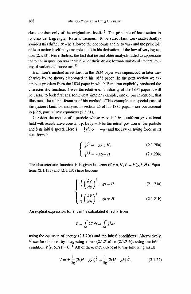
Consider the motion of a particle whose mass is 1 in a uniform gravitational field with accelerative constant g . Let y = b be the initial position of the particle and b its initial speed. Here T = iy', U = -gy and the law of living force in its dual form is

[ i Y 2 = - g y + H , (2.1.20a)

\ i b 2 = - g b + H . (2.1.20b)

The characteristic function V is given in terms of y, b, H, V = V (y, b, H). Equa- tions (2.1.15a) and (2.1.15b) here become

(2.1.2 1 a)

(2.1.21b)

An explicit expression for V can be calculated directly from

v = I' 2Tdt = L y 2 d r

using the equation of energy (2.1.20a) and the initial conditions. Alternatively, V can be obtained by integrating either (2.1.21a) or (2.1.21b), using the initial condition V ( b , b , H ) = 0.14 All of these methods lead to the following result

1 3 1 3 V=+--(2(H-gy))T r-(2(H-gb))7 3g 3g

(2.1.22)


Note that V simultaneously satisfies both (2.1.21a) and (2.1.21b). It is also easily seen that an integral giving y in terms of t may be derived by eliminating H from the two equations

After Hamilton derived the law of varying action he devoted several sections of the 1834 paper to what he called a “verification” of the integrals in (2.1.14). The partial differential equations (2.1.15) were initially introduced ostensibly in the aid of this endeavour. While today we might regard such a justification as unnecessary, the results in question are not without interest and serve to show the ways in which Hamilton was trying to consolidate and legitimate his new theory. They also provided a source of ideas for some of Jacobi’s innovations (including Jacobi’s theorem, discussed by us in 5 4.1). Hamilton first observed that if we take (2.1.14a) and use these relations to eliminate the 3n constants ai,bi,cj, we arrive at the equation of living force (2.1.6a). Thus if we begin with the equation of living force, derive the partial differential equation (2.1.15a), solve this equation to obtain V, we are led by the procedure just outlined back to the equation of living force. (Hamilton did not provide details, but he seemed to be saying that in the final relation of (2.1.14a), after 3n - 1 of the constants have been eliminated, the remaining constant appears in such a form that it disappears following partial differentiation. In our example above we have % = y, or ( 2 ( H - y ) ) 7 = y, whence the law of living force (2.1.20a) follows.)

Hamilton next showed that (2.1.14a) combined with the first partial differential equation (2.1.15a) leads back to the original equations of motion (2.1.3). Differ- entiating the first equation of (2.1.14a) with respect to t and using (2.1.15a) we have

1

a2v

J

(2.1.24) a au

= - ( U + H ) = -. axi axi Following the same procedure with respect to yi and zi we are led to


the equations of motion. Hamilton also felt that it was necessary to show that the intermediate inte-

grals (2.1.14a) are “consistent” with the final integrals (2.1.14b). Taking the time derivatives of (2.1.14b) we have

(2.1.25)

However, the left side of the first equation of (2.1.25) may be developed using (2.1.15a) as

a U+H Since *l = 0 the first equation of (2.1.25) follows, thus establishing the desired “consistence” in question.

Similarly, we are able to show that (2.1.14a) and (2.1.14~) are consistent. The time derivative of (2.1.14~) is

-(-) d a V = 1 . dt a H

(2.1.27)

However, beginning with (2.1.14a) and (2.1.15a) we have

(2.1.28) which is simply (2.1.27).

Throughout the preceding discussion Hamilton made use of (2.1.15a) and not (2.1.15b). Although these two equations were presented by him as jointly defin- ing the characteristic function, it is only the first which is used in his verification of the theory.

2.2 Hamilton’s Example of Characteristic Function

In section 13 of the “General Method” Hamilton illustrated the theory with the example of a binary system consisting of two point masses that interact mutually according to a specified force law. Consideration of this example will help us to understand how he intended his new method to be applied to concrete dynamical problems.


The two masses ml and m2 have coordinates ( x l , y l , z l ) and (x2,y2,z2) respectively and the potential function U is given in the form mlmzf(r) , where r is the distance between the particles. ( a l , bl ,c1) and (a2, b 2 , ~ 2 ) are the initial positions of ( X I 7 Y 1 7 Z I ) and ( X 2 , Y 2 , Z 2 ) - and

r = j ( x 1 - x2)2 + (y1 - y2)2 + (z1 - z2)2,

Hamilton noted that one could integrate directly the second order differential equations for the problem and express the characteristic function V in the term of 12 initial and final coordinates (xj,yi,zi) and (ai, bi,ci). He proposed instead to follow his new method, in which (1834a, p. 275) “to find the form of this function, we are to employ the following pair of partial differential equations of the first order:

combined with some simple considerations.” Hamilton continued: “And it easily results from the principles already laid down, that the integral of th~s pair of equations, adapted to the present question, is

V = ( x - + ( y - b)2 + ( z - c ) ~ . J2H2 (ml + m2)

Here (x ,y ,z) and (a,b,c) are the final and initial coordinates of the center of gravity of the system:

172 Michiya Nakane and Craig G. Fraser

The quantity p is

(2.2.4)

where the + sign holds if the distance between ml and m2 is increasing, and the - sign holds if this distance is decreasing. 8 is the angle between the initial and final radii ro and r. H and h are arbitrary constants and H I and H2 are auxiliary constants that sum to H , H = HI + H2.I5 Hamilton specified that h, HI , H2 may be determined from the three conditions

(2.2.5)

H=H1+H2. (2.2.7)

He gave no explanation of how (2.2.5) and (2.2.6) are derived or why they hold. Let be the quantity

Using his law of varying action he succeeded in deriving the integrals

(X-U)f---- 1 av a m2 ( P - g + h % ) > I xi=--=- midxi ml +m2 ml +m2

(2.2.8)

(2.2.9)

1 av a mi +m2

The derivatives of V with respect to xi,yi,zi give six “intermediate integrals” and those with respect to ai,b,,ci give six “final integrals” of motion for the binary system if one eliminates the three auxiliary quantities h, H I , H2 by conditions (2.2.5) to (2.2.7). Thus, the motion of the binary system is completely described in terms of the characteristic function. Hamilton observed (1834, p. 276)


that “the form of (2.2.2) may be regarded as a central or radical relation, which includes the whole theory of motion of such a system.” He verified this fact by deriving some key properties of the binary system - the velocity of the center of gravity is constant, the relative motion of the two masses occurs in a plane and the law of conservation of areas (angular momentum) holds.

An important question concerns how Hamilton arrived at the particular expression (2.2.2) for the characteristic function V. Although his own comments above might indicate that he obtained V as a solution of the partial differential equation (2.2.1), a closer examination of this and other examples suggests otherwise. Indeed, we support firmly the conjecture advanced by Conway and McConnell (1940, p. 614): “It seems probable that he first integrated the differential equations of motion and then evaluated by direct integration the right-hand side of the equation

Expressing this in term of the initial and final configurations he obtained the characteristic function in the appropriate form.”16

Let us consider in the example at hand how one would obtain the expression (2.2.2) for V using a process of direct integration. Since the relative motion of two bodies whose masses are ml and m2 is reduced to the motion of a fictional single body which has the so-called reduced mass of p = z, one treats the binary system as a fictional body moving around the center of gravity which itself moved freely under the action of no force. The total kinetic energy of the system T is the sum of that of the center of gravity (TI ) and that of the fictional body (Tz). Therefore the characteristic function of this system is

r t rf rt

2Tdt = J0 2Tidt + J0 2T2dt = V1 + V2. “ = l o (2.2. l o )

Since

ds 2 TI = ;(ml +m2)(2+y2+i2) = f ( m l + m 2 ) ( ~ ) = H2,

where ds = d w , we have

(2.2.11)

(2.2.12)

and

(2.2.13)

174

Thus

Michiyo Nakane and Craig G. Fraser

t vl = l 2 T , d t = 1 2H2dt = 2H2t

= &m1+ m 2 ) ~ z s

= J%GGj% (2.2.14)

To calculate V2, one introduces the energy equation for the fictional mass p written in polar coordinates,

T2 - mlm2f(r) = - P { L2 + r2b2} - mlm2f(r) = H I , 2

where -mlm2f(r) is the potential function and p = *. Then

From the conservation law of angular momentum p b = h, we have

6’ p p e 2 d t = yehdt = p h e , 6’ where h is a constant. From equations (2.2.15) and (2.2.17) we have

h2 L = / z { m l m 2 f ( r ) + H I } - r2e2 = -{mlm2f(r) + H I } - ;r d: P

Then

(2.2.15)

(2.2.16)

(2.2.17)

(2.2.

(2.2. 9)

Therefore V2 = p {he + lor pdr } . (2.2.20)

Adding V1 and V2 as given by (2.2.14) and (2.2.20) we obtain precisely equation (2.2.2) for V = VI + V2.

It is now clear why (2.2.6) and (2.2.7) hold. (2.2.7) asserts that the total energy H is the sum of HI and H2, the energies of the systems corresponding to V2 and V1 respectively. For V1 and V2 we also have from the law of varying action

(2.2.21)


The two partial derivatives may be evaluated from (2.2.14) and (2.2.20), and (2.2.6) follows immediately.

Our proposed reconstruction shows as well how (2.2.5) may be obtained, something that Hamilton did not explain at all. The derivation begins with the area law r;?0 = h, used above in the direct calculation of V2. We integrate 9 0 = h with respect to time:

r28dt = ht. (2.2.22)

av But = t from the law of varying action, and so

or.

Differentiating (2.2.23) with respect to time we obtain

. hi- P

r2e = -,

or, . hi- e = -

r*p ’ Integration of (2.2.24) in turn produces

or,

0 = 8 + 1’ g1

(2.2.23)

(2.2.24)

(2.2.5)

the relation Hamilton stipulated h must satisfy. In writings from 1776 and 1806 Lagrange had introduced the distinction - still

standard today - between a complete, general and singular solution of a first- order partial differential equation.” Typically, one tries to obtain a complete solution, containing as many arbitrary constants as there are independent variables. Consider the example of a particle with coordinates (n , y ) of mass 1 that moves freely in the plane under the action of no force. Equation (2.1.15a) is here

(2.2.25)

To integrate this equation, we first set H = h, where h is a constant. Next, we separate variables and set = a, where a is a constant. It follows that V =


ax + f(y), where f(y) is some function of y . Substituting V = ax + f(y) into (2.2.25), we obtain V = ax+ .J2h-;;Iz.y+p, where p is a second constant. The given solution V is complete, containing the three constants a, h and p. Noting that p is simply an additive constant arising because V does not appear in (2.2.25), we may express the complete solution in the form (up to an additive constant)

v = ax+ J T L 2 . y . (2.2.26)

An envelope of the family of solutions (2.2.26) is derived by solving (2.2.26) and = 0 simultaneously. This envelope is of course also a solution of (2.2.25). In

this case we obtain immediately

v = a q 9 q . (2.2.27)

Of course, V is precisely what we would find if we calculated V =

rectly : S

2Tdt = 2ht, but s = J 2 h . t and SO t = - J2h’ and consequently V = J 2 h d m . Thus the expression for V that results from a direct calculation is the same as the envelope derived from the complete integral.

In an appendix to volume two of Hamilton’s collected works Conway and Mc- Connell(l940, pp. 614-621) present a general theorem showing how Hamilton’s solution may be obtained as the envelope of a complete integral of the given partial differential equation. They apply their method to Hamilton’s 1834 example of a binary system. Although they had earlier suggested that Hamilton most likely derived the characteristic function by a direct calculation of the action integral, they here seem to imply that he may in fact have followed the method they propose. They write that their method “leads directly to a formula for the characteristic function which was used by Hamilton without any indication of how it arose,” and assert that this formula “actually suggests” the method in question. At the end of the derivation they observe that “the above expression for the characteristic function is exactly the form used by Hamilton.”

Conway and McConnell obtain Vl in the same way we derived (2.2.27) from (2.2.26), the given procedure being applied in this case with the three variables x - u, y - 6, z - c. For V2, they derive a complete integral, using an integration essentially the same as the one first presented by Jacobi in 184243, which we describe in $ 4.2. In this part of the deduction, relation (2.2.5) is introduced in order to derive the desired envelope from the complete integral.

Although Conway and McConnell’s investigation is of mathematical interest, it seems very implausible as a reconstruction of Hamilton’s original derivation,


if that is indeed what they intended. In none of his writings did Hamilton seem to show an awareness of the concept of a complete integral and envelope of a first-order partial differential equation.” In other examples that we shall consider, he explicitly employed a direct integration in order to obtain the principal function. ’

It seems difficult to suppose in the case of the binary system that he produced a complete integral, suppressed all evidence of what would have been a very notable result, and proceeded to obtain the characteristic function in the proper form by deriving an envelope from the complete integral. If he had used such a method he would have been powerfully motivated to describe it in detail, given its novelty and mathematical interest.

As we showed above, Hamilton’s formula (2.2.2) and the attendant relations (2.2.5) to (2.2.7) may be explained as arising from a direct calculation of the action integral, by means of the kind of “simple considerations” to which Hamilton referred. Hamilton’s primary goal was to show how knowledge of the characteristic function leads to a complete description of the binary system. The force of such a demonstration would have been rather diminished if formula (2.2.2) were itself seen to be calculated from the known solution of the differential equations of motion of the system. Hence Hamilton eliminated any discussion of how (2.2.2) was obtained, and did not provide a derivation of relations (2.2.5) to (2.2.7).

2.3 Generalized Coordinates and Lagrange’s Equations

In sections 7-9 of “General Method’ Hamilton introduced generalized coordinates and using them expressed the equations of motions in standard Lagrangian form. In this part of the essay appear some of the ideas that would become the basis of the canonical formalism set forth in detail in the 1835 paper.

Hamilton introduced generalized coordinates in the free or unconstrained case, so that the 3n rectangular coordinates XI, . . . ,xn, y1, . . . , yn9 z1, . . . ,zn are expressed as functions of the 3n coordinates 171, . . . , ~ 3 ~ . Then we have

(2.3.1)

a& dxi d7jj J V j

with similar relations for yi and zi. Noting that - = - etc., we obtain

(2.3.2)


where T is expressed in generalized coordinates as a function of the ml , . . . mn V I l . . . q 3 n and i l l , . . . , 7j3n. Then the law of varying action becomes

dT a TO a qi aei

6V = x - 6 q i - x - 6 e i + t 6 H l

where TO and ei are initial values of T and qi, and relations

( i = l , . . .13n) av a~ av - aT

- - - dqi a i j ’ dei dei’

(2.3.3)

(2.3.4)

are obtained. To derive the partial differential equation for V using the law of living force,

Hamilton reasoned as following: the function U depends on q1 l . . . , q3n9 UO on e l l . . . ,e3,,, T is a quadratic homogeneous function of z,. . . also q1,. . . q3,, and To is as a similar function of 2,. . . 2, involving also e l , . . . , e3,, . Hamilton seemed to recognize by analogy that T is a quadratic homogeneous function of the (g) ’s, since i i = & (g), etc. in rectangular coordinates. Furthermore equation (2.3.2) indicates that (qil R) correspond to ( X i , Yi Z i 1 mi&, miji 1 mi&), the latter being regarded as two kinds of independent variables in rectangular coordinates. Indeed, Hamilton treated (qi, g) as new coordinates and set

dT ai3n, dT involving

Note that regarding one half the living force as a function of the and the qi is quite different from regarding it as a function of the i l i and the qi. Here we find that Hamilton arrived at the primitive idea of the canonical coordinates which he would introduce more explicitly in his 1835 paper. In 1809 and 1810 Poisson and Lagrange already had set p = and had written Lagrange’s equations in simpler form (see (Liitzen 1990, pp. 641-42)). But the treatment of as a new coordinate variable was Hamilton’s original idea. Using relations (2.3.4) and the law of living force we obtain the two partial differential equations

(2.3.6a)

(2.3.6b)

(2.3.6a)

(2.3.6b)

Hamilton next demonstrated that Lagrange’s equations can be derived from the law of varying action. As the function T is a homogeneous function of order 2 in the variables Q i , we have

(2.3.7)


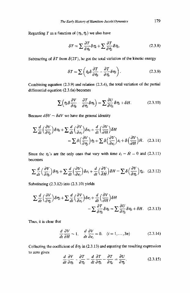
Regarding T as a function of (qi, Q i ) we also have

(2.3.8)

Subtracting of 6 T from 6(2T), he got the total variation of the kinetic energy

(2.3.9)

Combining equation (2.3.9) and relation (2.3.4), the total variation of the partial differential equation (2.3.6a) becomes

(2.3.10)

Because d6V = 6dV we have the general identity

Since the qi’s are the only ones that vary with time t i = becomes

= 0 and (2.3.11)

Substituting (2.3.12) into (2.3.10) yields

Thus, it is clear that

- 0. -1, --- ( i = 1,. . . ,3n) d dV d dV

dt d H dt aei (2.3.14)

Collecting the coefficient of 6qi in (2.3.13) and equating the resulting expression to zero gives

d dV d T - d J T J T - aU dt dqi dq i dt dQi &/i aqi’

(2.3.15) - - - - - - - - - - -


Hamilton (1834a, p. 261) observed that (2.3.15) “coincide in all respects (a slight difference in notation excepted), with the elegant canonical forms in the Mkchanique Analytique of Lagrange.” He emphasized that he had derived them in a new way using the properties of the characteristic function.

Hamilton observed that the analysis could also be carried out when geometrical relations or constraints connect the coordinates of the system. Interestingly, he noted that “the dynamical spirit is tending more and more to exclude” the assumption of such constraints, a point of view entirely in keeping with the Poisson-Laplace approach to mechanics, in which everything is explained in terms of forces acting on molecules and idealized mathematical constraints are rejected. Hamilton’s philosophical attitude here is also evident in the following remark (1 834, p. 262) “To those imaginable cases, indeed, in which the law of living force no longer holds, our method also would not apply; but it appears to the growing conviction of the persons who have mediated the most profoundly on the mathematical dynamics of the universe, that these are cases suggested by insufficient views of the mutual actions of body.”

At the close of “General Method,” Hamilton defined the “auxiliary function,”

S = V - t H = (T +U)d t . (2.3.1 6)

We have 6s = 6V - t 6 H - H a t . Substituting into this last equation the expression for 6V given by (2.1.13) we are led to the following equation for the variation of S:

l

Hamilton would subsequently call S the principal function. It was the principal function rather than the characterstic function that became standard in later Hamilton-Jacobi theory. From (2.3.17) he arrived at

= -H, ( i = 1, ... , n ) (2.3.18a)

From the conservation law of living force it follows that S satisfies the partial differential equations

(2.3.19a)

The Eurly History of Hamilton-Jacobi Dynamics 181

Here appears for the first time in the history of mechanics what in later science would become known as the Hamilton-Jacobi equation.

2.4 The Principal Function

Hamilton began the “Second Essay” of 1835 by deriving Lagrange’s equations directly from the fundamental dynamical equation (2.1.1).20 He proceeded to develop the canonical formalism in terms of a system of generalized coordinates, essentially taking off from some of the considerations he had introduced in the 1834 paper. He first noted that the variation 6T of T may be given in the form (2.3.8), where T is regarded as a function of the qi and the ?ji. He next introduced the expression for 6T given by (2.3.9). The quantity is expressed using the new symbol mi. We may now regard T as a function F of the qi and Di:

Note that it is necessary to introduce the new function symbol F in order to distinguish T regarded as a function of qi and f / i from this same quantity regarded as a function of mi and qi. Taking the variation of F and using (2.3.9) we arrive

Thus,

a ( F - U ) a F a m1 a mi - = ii, (2.4.3a) - -

since the potential function U does not depend on mi. Then Lagrange’s equations become

dDi d ( U - F ) __ - - .(i= 1, ..., 3n) dt a qi

(2.4.4)

Hamilton set

and obtained what later became known as the canonical equations,

( i = 1, ..., 3n) (2.4.6)

As we observed in 8 2.3, Hamilton’s invention of canonical coordinates and equations of motion was preceded by certain innovations of Poisson. Poisson


(1809) wrote Lagrange’s equations as

dpi dL - - - - dt aqi’

( L = T + U , i = 1, ..., n) (2.4.7)

where pi = g. In the same paper he observed that the perturbation function Q satisfied the relations

(2.4.8)

where (a1 ,... ,an) are the initial values of the coordinates and (a: ,... ,uL) are the corresponding initial velocities. Hamilton referred to Poisson’s paper at the beginning of the “Second Essay.” He apparently sought a simpler form of the equations of motion and succeeded in reducing them to a system of first order differential equation by setting = g. Hamilton’s initial attention in the 1834 paper would have been drawn to the g because of their appearance as coeffi- cients in the expression in generalized coordinates for the law of varying action (2.3.3). The idea of actually making the new variables seems then to have originated in the step (2.3.5) in that paper where he expressed T as a function F of the qi and $$. He needed to do this in order to derive his partial differential equations (2.3.6) for the characteristic function in terms of generalized coordinates. The idea was also contained in equation (2.3.9). The first canonical equations (2.4.6) follow directly from (2.3.9). The really critical moment in Hamilton’s thinking would then have occurred when he realized that (2.4.3b) allows one to write Lagrange’s equations in the form of the second equations (2.4.6).

Hamilton’s next step in the “Second Essay” was to show that his new method of obtaining a solution of the equations of motion was valid in the new coordinate system. He defined the “principal function” as

Note that in the canonical coordinate system we have

d H x m i - - H = 2T - (T - U) = T + U a mi

(2.4.9)

(2.4.10)

Thus the principal function S is simply the time-integral of what is today called the Lagragian. Hamilton set S’ = 2 and wrote the variation of the function S as follows,

(2.4.1 1)


We have

(2.4.13)

where (p i l e ; ) are the initial values of (mi,qi). Equation (2.4.13) is of course the counterpart for the principal function of Hamilton's law of varying action. We also have

(2.4.14)

From (2.4.13) and (2.4.14) Hamilton obtained the following set of 6n equations involving the principal function S

(2.4.15a) f3S - aqi '

as p i = -z.

m - -

( i = 1, ..., 3n) (2.4.15b)

Hamilton stated that (2.4.15) are integrals of equations (2.4.6), but he provided no verification of this assertion similar to the one he presented in 1834 for (2.1.14). One can confirm easily that these equations satisfy the second equations (2.4.6) by differentiating with respect to t and using (2.4.3b) and (2.4.10). However, a somewhat different argument is required for the first equations (2.4.6). The verification in question follows directly from the result known as Jacobi's theorem (see 5 4.1), although Jacobi's point of view was (as we shall see) rather different.

Hamilton next derived partial differential equations for the function S in the canonical coordinate system. He calculated

and obtained

from equations (2.4.6) and (2.4.15a). Then we have

(2.4.16)

(2.4.17)

(2.4.18) as at -+H=O.

184 Michiyo Nukune and Craig G. Fraser

Hamilton did not explicitly present (2.4.18). Rather, he indicated that -H =

- ( F - U ) is constant and presented the following two partial differential equations involving the principal function S:

It is important to note that Hamilton’s derivation of (2.4.19) is quite different from his earlier derivation of equations (2.1.15) or (2.3.19). To obtain the latter, he used the law of varying action and the law of living force. By contrast, the process by which (2.4.19a) is derived does not require the law of living force and remains valid when the system is described in term of time-dependent potentials. Hamilton himself showed no consciousness of this fact, and indeed repeatedly stated that his method only applies when the law of living force is valid. He used this law to obtain (2.4.19b), an equation that he regarded as essential to a full description of the mechanical system. The second partial differential equation, in its genesis in his earlier researches, indicated the importance of (2.3.17), the law of varying action for the principal function. The form of this relation for a canonical coordinate system - given as (2.4.13) - involved the important idea of varying both the initial and final points of the path. Since equation (2.4.19a) didn’t invoIve the initial values, he added (2.4.19b) using the condition H =

constant in accordance with the law (2.4.13). The origin of Hamilton’s principle is worth a mention in passing. In develop-

ing his theory of principal functions, Hamilton observed that Lagrange’s equations are a direct consequence of the condition

6s = 0, (2.4.20)

where the end positions are fixed. The variation of S becomes

If the extreme points are fixed, the first term of the right hand becomes 0. Then we obtain Lagrange’s equations directly from (2.4.20) (Hamilton 1835, p. 99).

Thus the function S gives rise to the integrals of the problem as well as to the differential equations themselves. The variational law (2.4.20) had not occurred in earlier mechanics, because the quantity T + U appearing in the integrand of S has no particular physical significance or meaning. Hamilton arrived at (2.4.20) essentially from formal considerations, and he seemed to understand this law in


quite formal terms. For him it was a byproduct of the theory, rather than the fundamental axiom that it is in modem dynamics. Thus, he constructed his new formalism from the equations of motion, rather than from the variational principle itself. In this respect his dynamical theory was quite different from his earlier work in geometrical optics. In the latter he had begun by deriving Fermat’s variational principle of least time from the laws of reflection and refraction, and had then made the Fermat principle the basis for his whole theory - from it he derived the Malus orthogonality condition and the partial differential equation satisfied by the characteristic function. The principle of least action or “Hamilton’s principle” (2.4.20) played no such comparable role in Hamilton’s dynamics.*’

2.5 Hamilton’s Approximation Method

From the viewpoint of obtaining integrals of the given partial differential equations, one may well ask what advance or improvement results from the method of principal functions. A very natural approach to the integration of (2.4.19a) would be to let H = F - U = h, where h is a constant. It follows immediately that S = V - ht, where V is a function of xi , y i , zi , ai, bj, ci. From this relation one sees that = g, and so on. To complete the integration we substitute the partials of V into the equation h = F - U . We are led in this way directly back to the characteristic function, equation (2.1.15) and the corresponding theory of the 1834 essay.

Hamilton was motivated to develop the method of principal functions not out of a mathematical interest in the integration problem, but because of his interest in perturbations in physical astronomy, as celestial mechanics was then called. In a letter of October 17, 1834 to John Herschel, Hamilton commented on the direction of his research:

= g,

I used, as you will find, throughout the greater part of my First Essay, a Characteristic Function V, more closely analogous to the optical function which I had denoted by the same letter, and expressing, as in Optics, the dependence of the quantity called Action on the final and initial co-ordinates. But this function V in Dynamics involved also, as an auxiliary quantity, the constant H in the known expression for half the living force of a system; and the eliminations by which I was obliged to get rid of this auxiliary constant, and to introduce the time in its stead, made the method more embarrassing than it is in its present form, especially in questions of perturbation. (Graves V.2 1885, p. 114)

For Hamilton, the importance of the theory based on the principal function resided in its application to problems of perturbation. Such problems were approached by him using a method of successive approximation. An initial solution, derived for the “undisturbed” motion, is used in developing a better approximation that includes a disturbing force; the solution that is obtained can be further refined by the inclusion of higher-order disturbances. The resulting


approximation procedure for Hamilton constituted the main application of his theory to dynamics.

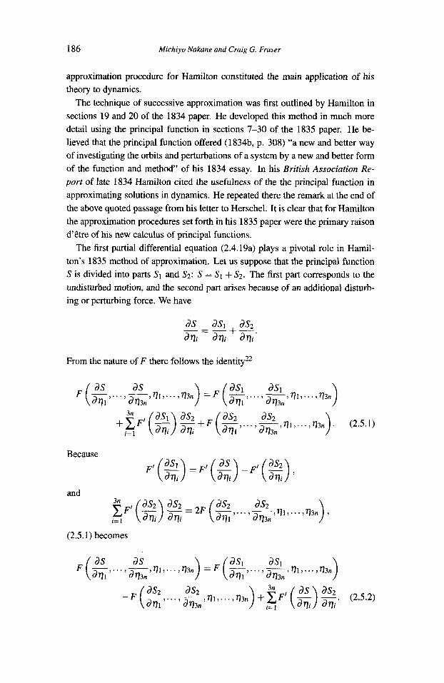
The technique of successive approximation was first outlined by Hamilton in sections 19 and 20 of the 1834 paper. He developed this method in much more detail using the principal function in sections 7-30 of the 1835 paper. He believed that the principal function offered (1834b, p. 308) “a new and better way of investigating the orbits and perturbations of a system by a new and better form of the function and method” of his 1834 essay. In his British Association Re- port of late 1834 Hamilton cited the usefulness of the the principal function in approximating solutions in dynamics. He repeated there the remark at the end of the above quoted passage from his letter to Herschel. It is clear that for Hamilton the approximation procedures set forth in his 1835 paper were the primary raison d’gtre of his new calculus of principal functions.

The first partial differential equation (2.4.19a) plays a pivotal role in Hamil- ton’s 1835 method of approximation. Let us suppose that the principal function S is divided into parts S1 and S2: S = S1+ S2. The first part corresponds to the undisturbed motion, and the second part arises because of an additional disturbing or perturbing force. We have

From the nature of F there follows the identity22

Because

and

(2.5.1) becomes


From the canonical equations (2.4.6) and the integrals (2.4.15) it follows that

Hence

Consider now the partial differential equation (2.4.19a); with S = S1+ S;! it becomes

(2.5.3) may using (2.5.2) and (2.5.4) be put in the form

Integrated, (2.5.5) becomes

If S1 is a reasonable approximation to S then S2 and 3 are small and the second integral on the right side of (2.5.6) is neglibible. S2 = AS1 is then the correcting factor that must be added to S1 to better approximate S:

Suppose now that S1 = S1 ( t , q1, . . . , q 3 n , e l , , . . ,e3n) is given.Then we are able to obtain the qi as functions of t , e l , . . . , e3n,p1 , . . . ,p3n from the integrals

(2.5.8)


Inserting the resulting expressions for 77i into the integrand of (2.5.7) and car- rying out the integration we compute SZ. Next, using (2.5.8) again, we replace the pi in this expression and obtain S2 in normal form as a function of t , 7 1 1 7 . . . ,773”, el , . . . , e3n. The desired final expressions for the qi are then given, to a second approximation, by the integrals

(2.5.9)

Evidently the whole process may be repeated; as Hamilton observed (1835, p. 102), “And when an improved expression, or second approximate value S1+ AS1, for the principal function S, has been obtained, it may be substituted in like manner for the first approximate value S1, so as to obtain a still closer approximation, and the process may be repeated indefinitely.”

Hamilton next introduced some general considerations concerning perturbation problems. Decompose H into two parts H = H I + H2. with

The canonical equations are here

If the quantity H I corresponds to the undisturbed motion, and if we assume that the effect of the disturbance is relatively small, then a good approximation to the motion is given by the equations

(2.5.12)

To go from the undisturbed motion as given by (2.5.12) to the actual, disturbed motion is called by Hamilton “a Problem of Perturbation.” A solution of (2.5.12) will be given in the form

The component S1 of S for the undisturbed motion is then

(2.5.14)


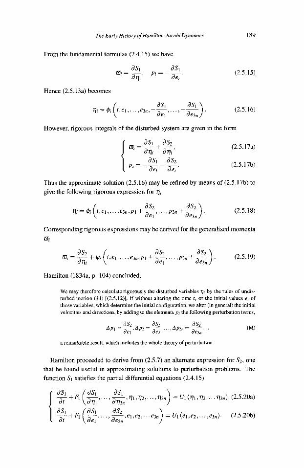
From the fundamental formulas (2.4.15) we have

Hence (2.5.13a) becomes

(2.5.15)

(2.5.16)

However, rigorous integrals of the disturbed system are given in the form

(2.5.17a)

(2.5.17b)

Thus the approximate solution (2.5.16) may be refined by means of (2.5.17b) to give the following rigorous expression for 77;

(2.5.18)

Corresponding rigorous expressions may be derived for the generalized momenta mi

Hamilton (1834a, p. 104) concluded,

We may therefore calculate rigorously the disturbed variables qi by the rules of undisturbed motion (44) [(2.5.12)], if without altering the time t , or the initial values ei of those variables, which determine the initial configuration, we alter (in general) the initial velocities and directions, by adding to the elements pi the following perturbation terms,

a remarkable result, which includes the whole theory of perturbation.

Hamilton proceeded to derive from (2.5.7) an alternate expression for S2. one that he found useful in approximating solutions to perturbation problems. The function S1 satisfies the partial differential equations (2.4.15)


(It is worth noting that although the second of these equations played no role in Hamilton’s method of approximation, it was presented by him in accordance with his practice of always giving the principd function in terms of both partial differential equations.) By (2.5.20a) the fundamental formula (2.5.5) becomes

Because the quantity F (2,. . . , Zl q1 l . . . , ~ 3 ~ ) is small, (2.5.21) reduces to

Because 3 is small we may employ the approximation

in (2.5.22). Hence the latter equation may be written

or, since -Hz = U2 - F2, t

S2 = - 1 H2dt. (2.5.23)

Hamilton devoted some seventeen pages of the 1835 essay to showing how his method may be applied to the motion of a single particle acted upon by a force. He also included here the detailed treatment of an example involving a specific potential function. Although he was primarily interested in what he called “at- tracting and repelling systems” consisting of several particles, he believed that this fairly simple example served to illustrate the important features of his theory. He spared no detail in his account; we shall here only describe some of his main results.

In a system consisting of a single particle of unit mass the coordinates (771,

q2, q 3 ) of the particle are simply its Cartesian coordinates x,y,z. The potential function is assumed to have the form

(2.5.24)

where g, p, v are constants. (Later, on p. 130, Hamilton explained that this example approximates the situation of a projectile moving in a void. If we assume the


earth is a sphere of radius R and r is the distance of the projectile from the earth’s center then U = gR2 (i - i), where g is the value of the accelerating force of gravity at the earth’s surface. Consider a rectangular coordinate system with origin on the earth’s surface in which the z-axis is directed vertically outwards. Then we have

r = Jw, gz2 d 2 + Y 2 )

2R ’ u = -gz + - - R2

where we have in the second equation neglected terms of second and higher order in E . ) 1

In the example at hand the function H is

(2.5.25)

Hamilton wrote down the canonical equations for the system and integrated them directly to obtain the “rigorous” solution23

1 1 H = - ( D ; + 2 + D:) +g773 + ~ ( ~ ~ ( 7 7 : + 77;) + V2~:}.

P1 771 = el cospt + - sinpt,

7J2 = el cos p t + - sin p t ,

773 = el cos Vt + - sin Vt + -vers Vt.

(2.5.26) E 2 .

k . g V V2

Introducing (2.5.26) into F + U , performing the integration S = (F + U ) d t , and substituting for the pi using (2.5.26) in the resulting expression, we are led to the following “rigorous” expression for the principal function S ;

l g2t 2v2 2 tanpt 2 tanvt

p . (vi -el)’+ (v2 - e2)2 v (v3 - e3)’ s=-+- + - . Pt Vt

-p(lllel+772e2)tan- 2 - V ( q 3 t 5) (e3+ $) tanT. (2.5.27)

Hamilton observed that S satisfies the two partial differential equations (2.4.19), where U is given by (2.5.24). He further observed that “[if the] form [of S ] had been previously found, by the help of this pair, or in any other way, the integrals of the equations of the motion might (by our general method} have been deduced from it” by means of the integral (2.5.24). (1835, p. 120) (Emphasis in the original. The quoted passage was repeated by Hamilton like a catechism every time in the 1835 paper that he arrived at an explicit expression for the principal function S).

Hamilton’s next step was to apply his approximation method to the system, showing that the results obtained agreed with the rigorous solution (2.5.26), if


the latter is expressed as a power series and higher-order powers of p and v are neglected. Divide H into two parts:

Suppose p and v are small quantities so that HI dominates in H (the undisturbed case).The canonical equations (2.4.6) for H I are

These equations are easily integrated directly:

711 = el + P I t , 712 = e2 + pz t , 713 = e3 + p3c - kgt2,

Dl =PI1 a = p 2 , @3=p3-g t , (2.5.31)

where el, e2, e3, p1, p2 , p3 are as usual the initial values of 711 , 712, q 3 O J ~ , 9 g respectively. Hamilton calculated the principal function S1 using these results,

The function satisfies the two partial differential equations

as as as %+:{($) +(&) +($) }=-ge3 . (2.5.33b)

Here the integrals

(2.5.34)

actually coincide with equations (2.5.3 1). The goal now is to refine the preceding approximate solution by means of for-

mula (2.5.23). Take H2 as defined by (2.5.29) and introduce into this expression the values for qi given by (2.5.31):

P’ V L 1 2 2 -H2 = -- {(el + p l t ) 2 + (e2 + p ~ t ) ~ } - - (e3 + p3t - ?gt ) . (2.5.35) 2 2


Performing the integration - H2dt and substituting for the pi using (2.5.31) in the resulting expression we are led by (2.5.23) to the following expression for the principal function S2:

I’

The corrected function SI +S2 is obtained by adding (2.5.32) and (2.5.36). Refined expression for the functions qi are in the case given by (2.4.15b),

or, more directly,24

771 -el t

712 - e2 t

773 - e3 I

+ + +

1 2

” ( e l 3 + p),

(2.5.37)

Hamilton observed that (2.5.37) coincide with the rigorous integral (2.5.26) if the latter are developed as far as the squares of the quantities p and v; similarly Si + S2 coincides with S as given by (2.5.27) if the latter is expressed to the same degree of accuracy.

Hamilton continued by substituting S1+ S2 for S1 and setting S = S1+ SZ + S3.

The approximation process in this case yields an expression for S of improved accuracy, including powers of p and v up to six. Hamilton also discussed in some detail “the theory of gradually varying elements,” i.e., the variation of the orbital constants, as it pertains to the example under consideration; we shall however not follow him in his exploration of this subject.

In surveying Hamilton’s treatment of perturbation problems we are led to some general observations concerning his method of successive approximation. It is first clear why he preferred the method of principal functions over the method of characteristic functions. One is primarily concerned in physical astronomy with obtaining the coordinates and momenta of the bodies as functions of the time. The characteristic function V is given in terms of the qi and H, and so t must be introduced and H eliminated by means of the relation = t . As Hamilton


observed in his letter to Herschel, this is not always easy to do. Consider the system described by equations (2.5.28), and for simplicity specialize the motion to one dimension, so that H1 = itiT: + g773. This is precisely the example we considered in 0 2.1, with H = HI, y = 773 and b = e3. The characteristic function in the present notation is

The integral of motion is given in the form

It is necessary to eliminate H1 from the relation

av, 1 ‘ 1 I

aH1 g g t = - = - (2(H1- 8773)) - - HI - ge3)) ’,

a step that is not entirely straightforward. The difficulty here is of course much more pronounced in the complicated n-body systems of actual interest to Hamil- ton.

The preceding consideration also explain why Hamilton was not strongly motivated to investigate the problem of integrating the partial differential equation

+ H = 0. To do so would lead directly back to the characteristic function and a solution that involves the relation = t . Thus, although the partial differential equation (2.4.19a) is basic to his approximation procedure, Hamilton never in the various systems and examples examined actually integrated this equation (or the companion equation (2.4.19b)).When he produced the principal function in “rigorous” form, he did so by integrating the associated canonical differential equations of motion. In order to get the approximation procedure started it is necessary to find S1; in the examples considered this is again done by direct integration of the equations of

Hamilton grouped the partial differential equations (2.4.19a) and (2.4.19b) to- gether, and repeatedly stressed their joint fundamental character in the theory. Nevertheless, only (2.4.19a) is used in the approximation of this method. Anal- ogous remarks apply to (2.1.15a) and (2.1.15b) and the approximation method laid out in sections 19-20 of the 1834 paper.

Unbeknownst to Hamilton, his method as presented in section 7 of the 1835 paper does not require the principle of living force - it applies equally to non- conservative systems containing time-dependent forces. Finally, Hamilton assumed that the principal function S has a specific form: it is a function of time t , the initial coordinate values ei, and the final coordinate values qi. The possibility of other forms for S was not envisaged by him. Again, analogous remarks apply to the function V in the 1834 paper.


3 A New Integral of the Three-Body Problem: Jacobi’s Study of Dynamics in 1836

The “Verzeichniss siimmtlicher Abhandlungen C. G. J. Jacobi,” contained in Jacobi’s Gesammelte Werke (Werke 7, pp. 425-440), indicates that Jacobi began to publish work on dynamics in 1836. Before 1836 he was engaged primarily in number theory and the theory of elliptic functions, subjects which he continued to investigate throughout his life. He also studied the general theory of first order partial differential equations and published two papers in this subject in 1827.

Jacobi’s research interests prior to 1836 also included topics in mechanics. In the famous letter to Legendre of 1830 in which he extolled the virtues of pure mathematics, Jacobi also mentioned that he was working on problems in celestial perturbations, work which he said involved the new theory of elliptic functions.26 Leo Koenigsberger has pointed out (1904a, pp. 19-20) that Jacobi applied his results on elliptic functions to problems of mechanics and astronomy. Koenigsberger also indicates that Jacobi wrote a letter to his brother in December 1832, saying that he had obtained many interesting results from his study of the works of Newton, Maclaurin, D’Alembert, Lagrange, Ivory and Gauss on the attraction of ellipsoids. Jacobi was also interested in mechanics during these years. In 1834 he published an article on the equilibrium figures of a rotating fluid mass in the Annalen der Physik.

On July 14, 1836 Jacobi submitted a remarkable result on mechanics to the Berlin Academy (1 836a). He succeeded in deriving a new integral for the three- body problem, the so-called Jacobian integral of the restricted three-body problem. Since Newton, mathematicians had tried to solve the three-body problem under various special conditions, but little progress had been made since the results of Lagrange in the 1770s. Jacobi’s integral was something of a break- through, and it was acknowledged as such by prominent contemporary observers, including Cayley ((1857, p. 15), (1862, p. 541)) and Joessph Liouville (1856, p. 260-264). In his 1899 survey of the three-body problem Edmund Taylor Whit- taker wrote that Jacobi’s result had occupied a prominent place in research of the nineteenth century (1899, p. 123).

Jacobi’s original restricted system was composed of two bodies revolving around their center of gravity in circular orbits under the influence of their mutual attraction, and a third body without mass, which is attracted by the two bodies but does not disturb their motion. More precisely, he considered the motion of a point (which is taken to represent a body such as a comet) attracted by the sun and perturbed by a planet. The sun has mass M and stays at the origin of an (x,y,z)-coordinate system. The planet has mass m’ and moves around the sun describing a circle with constant angular velocity in the xy plane. a1 is the radius of the orbit and n’ is the angular velocity of the planet. (x,y,z) are the coordinates


Jacobi s three-body system

I Z point mass of sun = M

mass of planet = m'

mass of point = 1

I i Figure 1

of the point whose mass is 1. (See Figure. 1). For this point, Jacobi gave the following integral of motion:

1 + ml{

x2 + y2 + z2 - 2al (xcosn't +ysinn't) +a:

x cos n't + y sin n't } +const. (3.1) - a:

The assumptions in place here are reasonable in discussing a three-body system consisting of the sun, Jupiter and a comet because the eccentricity of Jupiter is only 1/20 and the mass of the comet is very small. Jacobi also communicated the same result to the Paris Academy (1836b) on July 18, 1836, without proof.

In addition to its interest as a solution of the three-body problem, equation (3.1) has a remarkable property from our standpoint. The right side of equation (3.1) reminds us of a potential function, one moreover that explicitly involves


the time. Indeed, the law of conservation of living force fails in this particular example, and it is significant that Jacobi’s first major result in mechanics involved such a non-conservative system. As we shall argue later, this fact would influence his response to Hamilton’s contemporary work in dynamics.

As indicated earlier, Jacobi’s integral was regarded by mathematicians of the period as an important special solution of the three-body problem. The integral occupied a significant place in later writings of such celestial mechanicians as Franqois Felix Tissererand (1 896, pp. 203-205), George William Hill, George Howard Darwin, and Forest Ray Moulton (1914, pp. 280-281)?7 In modern books the integral is derived using rotating coordinate systems by means of formulas that connect acceleration and force in such systems. Jacobi himself provided no derivation of the integral - he often made public important mathematical results without explaining how he arrived at them. However, we can pretty confi- dently reconstruct his derivation from circumstantial clues and from the evidence of the fifth lecture published in his Vorlesungen of 1866 (pp. 31-43).

First, it is notable that Jacobi in his 1836 communication mentioned James Ivory and the Philosophical Transactions, this occurring in a reference at the beginning to a result that Jacobi had presented in an earlier publication. The editorial notes to Jacobi’s Werke identify this earlier paper as “Uber die Figur des Gleichgewichts” dated October 4, 1834. ( Werke 4, p. 540). Although this piece was closely connected to work published by Ivory in 1831, Jacobi did not mention Ivory in the 1834 article. His explicit citation of Ivory in the 1836 communication would suggest a renewed awareness of the Englishman’s research.

Certainly a paper of Ivory’s that is directly relevant in the background to Ja- cobi’s 1836 result is “On the Theory of the Perturbation of the Planets,” published in the Philosophical Transactions in 1832. Ivory’s underlying goal was to reduce somewhat the long train of calculations that are involved in the study of perturbations. In order to carry out this investigation, he first obtained the differential equations describing the motion of one of the bodies of a given three-body system in terms of a potential function. The system consists of the sun S and two planets P and P’. The coordinates are arranged in such a way that S is located at the origin. (x,y,z) are the coordinates of P and (x’,y’,z’) are the coordinates of P’. M, rn, m’ denote the respective masses of S , P, P’, r and r‘ are the respective distances of P and P’ from S and p is the distance between the two planets.

The force of attraction between S and P is f , where p = M + m. The resolved parts of this force acting along the directions of x,y,z are


The planet P‘ attracts S with force 5, of which the resolved parts are

m‘x’ m‘y‘ m‘z‘ r‘3 ’ r‘3 ’ r‘3 * - --

The planet P‘ attracts P with force 5, of which the resolved parts are

m’(x’ - x ) m‘(y’ - y ) m’(z’ - z )

P 3 ’ P 3 ’ P 3 .

(3.3)

(3.4)

In addition to the interaction given by (3.2), the difference of these last two equations (expressing forces having opposite directions) corresponds to a force acting to alter the place of P relative to S. Hence the equations of motion of P are

’ d2x px m’(x!-x) m’x’ -+-= --

-+-= --

d2z p z m‘(z ’ -z ) m’z’ -+-= --

dt2 r3 P 3 $3 ’ d2Y PY m’(y’-y) m’y’ dt2 r3 P 3 r‘3 ’

dt2 r3 P 3 $3 .

(3.5)

If we assume

these equations may be written

1 d2x x dR -_ +-=- p dt2 r3 d x ’ 1 d2y y dR _- + -= - p dt2 r3 d y ’

1 d2z z dR ---+-=-. y dt2 r3 dz

(3.7)

In his earlier purely mathematical article “On the theory of the elliptic transcendents” (1 831 b) , Ivory repeatedly mentioned results of Jacobi, and it is reasonable to assume that Jacobi in turn would have been attentive to the English- man’s research. Certainly the formulas (3.7) in Ivory’s 1832 paper were directly relevant to Jacobi’s derivation of an integral for the three-body problem. In Ja- cobi’s case the function R becomes

1’ xcosn’t +ysinn’t - 1

JX2+y*+z2-~u~(xcosn’r+ysinn/r) +a: 4 (3.8)


where p in Ivory’s result is substituted for M as the mass of the point is negligi- ble. The potential function U becomes

M + M R , @TjG7 (3.9)

which satisfies the equation

--+--+-- +- (3.10) a x dt ay dt d ( i d z ) dz dt

Note that in Jacobi’s example the function U explicitly involves the time, whereas in Ivory’s investigation U was a function of the spatial coordinates alone. Because is non-zero, the principle of living force does not hold: the system is non-conservative. In addition, equation (3.10) can not be integrated in the usual way. Jacobi succeeded in obtaining a solution using an ingenious method that he would later describe in the fifth of his 1866 lectures (pp. 3143). This lecture was devoted to the principle of conservation of areas (angular momentum) and to a variant of this principle that holds for time-dependent potentials.

In the Vorlesungen Jacobi adopted a Lagrangian virtual-work approach to mechanics. In the fifth lecture he separated the time-dependent part of the potential function from the whole part. We denote by Ul the part that does not contain the time; by 172 the other part, which contains the time, and set U = U1+ U2. Taking the total derivative of U and replacing x, *,

a t dU -=( d U d x d U d y dt

au au au d2x d2y d2z with ;i;r, @, ;i;z, we obtain

(3.1 1) d2x d2y d2z au2 - 6 x + -6 + -6z = 6Ul+ 6u2 - -6 t . dt2 dt2 dt2 at

Our main interest is how Jacobi would treat - 9. He introduced the so-called cylindrical coordinates,

x = rcosv, y = rsinv, z = z . (3.12)

The potential function becomes

M 1 - r cos t2- n‘t ) 1 lJ= ~

d m +m‘{ 4 r2 + u: - 2alrcos(v - n’t) +z2 1

(3.13) Jacobi considered a rotational variation about the z-axis subject to the condition that r and v - n’t remain unchanged. Consequently neither U1 nor U2 is varied. As the relation 6v = n’& holds for this variation, he set

6 x = -rsinv6v = -n’y6t, 6y = rcosv6v = n‘x6t, 6z = 0.

(3.14)


Equation (3.11) becomes,

(3.15)

which is a modified form of the principle of the conservation of areas.28 Equation (3.15) is the key relation in Jacobi’s method. With it he easily integrated the eauation

(3.16) d x d 2 x d y d 2 y d z d 2 z dU1 dU2 aU2 -- +--+--=-+--- dt dt2 dt dt2 dt dt2 dt dt at ’

and obtained

If we replace U I + U2 by (3.9), we obtain Jacobi’s integral. The integral (3.1) follows directly from the theory set forth in the Vorlesungen.

Although Jacobi’s lectures on mechanics were given in 184243, the following passage from his paper “Zur Theorie,” dated November 29, 1836, (1 837a, p. 8 l), provides further evidence that he derived (3.1) by means of the process outlined above:

Here one can seek the motion of a mass point which is attracted by two bodies that move simultaneously around their common center of gravity with the same angular velocity. One has then two differential equations of the second order whose forces explicitly contain the time, therefore one can apply neither the principle of areas nor the principle of living force.. .But I have shown that a certain combination of the two principles holds.

Jacobi clearly valued the method laid out in the Vorlesungen not just because it led to a new solution to the three-body problem, but also because it provided a general approach to problems involving time-dependent potentials. He discussed dynamical systems whose potential functions explicitly depend on time in his two papers of 1837, “Zur Theorie” and “iiber die Reduction.” To emphasize the wide applicability of his theory, he referred to examples involving time-dependent potentials.

In conclusion, it should be noted that the example considered by Jacobi is representative of only one type of non-conservative dynamical system. There are of course many reasons why the law of conservation of living force may fail - the system may be subject to friction or dissipative effects, there may be forces present that depend on velocity, or the forces themselves may involve time. Jacobi’s system is of the last sort. The system is analysed using a model in which the law of living force does not hold. Such examples occur frequently in engineering, where some of the bodies of the system are supposed to be subject

The Early History of Hamilton-Jacobi Dynamics 20 1

to uniform, externally imposed motions.29 The fact that the law of living force fails does not entail any actual physical violation of energy conservation - it is just that the system is isolated and idealized for the purposes of analysis in terms that involve a time-dependent potential.

4 Jacobi ’s Dynamics (1 837)

4.1 The Presentation of Hamilton’s Theory

According to Koenigsberger (1904b, pp. 198-199), Jacobi wrote to his brother in a letter of 17 September 1836 stating that Hamilton’s papers had led him deeply into the study of important dynamical subjects. This would suggest that Jacobi read Hamilton’s papers in the summer of 1836, after he sent his letter on the three-body integral to the Paris academy. Although many Continental scientists of the period would not have read English journals, Jacobi was - as we saw in the preceding section - in the custom of consulting the Philosophical Trans- actions. He quickly arrived at some observations of Hamilton’s work which he (1837a, pp. 76-77) reported in the second half of his paper “Zur Theorie:”

Hamilton has shown that mechanical problems for which the theorem of living force is valid may be reduced to the integration of a partial differential equation of the first order. He actually proposed the integration of two such partial differential equations, but it is easy to show that it is sufficient to know any complete integral of one of them. It is also easy to extend his result to the case where the force function, that is the function whose partial derivatives give the forces, explicitly contains the time. In this case the theorem on living force is not valid but the principle of least action continues to hold.

Jacobi’s observation about the applicability of Hamilton’s method to time- dependent forces was developed in some detail in his 1837 paper “iiber die Re- duction.” Here Jacobi distilled the content of Hamilton’s method, adding some new results of his own. The essential result that he presented may accurately be called “Hamilton’s theorem,” though neither Jacobi nor later writers used this term. Jacobi defined the function S as

(4.1.1)

where, in this case, the potential function may explicitly contain the time as a variable. (Nowhere in the paper did Jacobi employ Hamilton’s terms “principal function” and “characteristic function.”) In taking the variation of an analytical expression, Jacobi followed the process he had employed in the first part of “Zur Theorie” in his ground-breaking study of sufficiency theory in the calculus of variations. Assume the problem is to maximize or minimize the definite integral


J = f f ( t , x , i ) d t . The requisite function x( t ) will be a solution of the Euler- Lagrange equation, a second-order ordinary differential equation. Hence x = x ( t , a , P ) , where a and P are arbitrary constants. We suppose that the constant a is used in parameterizing a family of comparison curves x = x ( t , a). The variation of any expression J involving x( t , a) is then defined as g d a .

Consider now a mechanical system consisting of n particles mi that move freely and interact according to the following 3n differential equations

d2xi dU d2yi dV d2zi dV (4.1.2)

where the potential function V is a function of the xi,yj,Zj and t . (We describe only the free case; Jacobi also considered constrained systems.) It is evident that U may be expressed as a function of t and the 6n arbitrary constants a1 , . . . , ajn that arise in the integration of (4.1.2). For a variation defined with respect to one of these constants a the fundamental equation (2.1.1) becomes

m.- = - m.- = - m.- = - ’ dt2 d ~ i ’ ‘ dt2 dyj’ dt2 dz i ’

dU

i - - dt

- Tmi (dxi -- d 2 X i dyi a2yi + --). dzi d2Zi (4.1.3) +-- dt d a d t dt d a d t dt d a d t

This equation may be rewritten in the form

Taking the variation of S defined by (4.1.1), we obtain


= Fmi ( X i $ +y.& +Z.dL') 'aa 'da

Equation (4.1.5) is valid for each arbitrary constant a k (k = 1 , . . . ,6n). Con- sider the following designations,

(4.1.6) constitute the most general variations that can be achieved when each of the 6n constants of integration is allowed to vary. (It is worthy of note that Jacobi defined the variations in such an explicit way. Some important issues associated with this definition are identified in the discussion that follows equation (4.1.12).) By multiplying each side of (4.1.5) by d a k and summing from k = 1 to k = 6n we obtain3'

Jacobi next explained that S is a function of t , x i l ~ i l z i and the initial values ail bi,ci. He reasoned as follows. The quantities xi,yj,zi are functions o f t and the a1 , .. . , as,. It is therefore evident that S is a function of the a1,. . . , &, and t. However, the aj can by inverting the given relations be expressed in terms of t ,xi , y i , zi and ui, bi, ci. Whence it follows that S itself is a function of these quantities. (It is an indication of Jacobi's critical sense that he explicitly spelled out this argument - the reasoning in question was regarded by Hamilton in a tacit way as intuitively evident.) Taking the variation of S in this form we obtain

It follows from (4.1.7) and (4.1.8) that

(4.1.9)


Differentiating S as given in (4.1.1) with respect to t we obtain

= u + - 1 c m; (2 + ji 2 2 + ii . dt 2 ;

(4.1.1 0)

However since S = S ( t , x l , . . . , x , , y l , . . . ,yn ,zl,. . . ,z,) the derivative of S is given in the form

(4.1.1 1)

Comparing (4.1.10) and (4.1.1 1) and using (4.1.9) we arrive at

- - ”+q”)2+ at mi ax; ( ” ) 2 + J Y ; (ds)2], azi

or

(4.1.1 2) as 1

In the Vorlesungen Jacobi (1 866, p. 147) would refer to (4.1.12) as “the Hamil- tonian equation,” a designation that is indeed more apt than the modem name “Hamilton-Jacobi equation”.

Before turning to a critical examination of Jacobi’s derivation, we call attention to a particular technical point concerning the variational process employed by Hamilton and Jacobi. The reasoning involved in (4.1.10) to (4.1.12) may be summarized as follows.

For simplicity, we consider only one point whose mass is m with one depen-

dent variable. Let S = f(t,x(t),x(t))dt. Then 2 = f. But - + 2.i. so dS - ds I’ we have

Now we have seen that 6s = $$ax = mi. Since S = s ( t , x ) we have 6s = E. Hence =

f = id + U = & ( E ) 2 + U , and so weobtain U = 9 + & ( g ) 2 , theHami1- ton-Jacobi equation.

In later calculus of variations it became standard to use variations in which t as well as x is varied. In this approach the variation of S is given by the endpoint

= mi. Substitution into (*) produces f = as + I ( z) as 2 . But

formula in the form

so that


As usual we have = mi and consequently 2 = $$ = ink. Substitution into the first equation of (**) leads to the Hamilton-Jacobi equation, as before. 31

We turn now to some reflections of a critical sort concerning Jacobi’s theory. Although Jacobi was reproducing the essential steps of Hamilton’s method, his own account served to call attention to some important aspects of this method. Jacobi derived (4.1.10) in a traditional setting involving the coordinates and time in which the equations of motion are second-order differential equations. His development showed that Hamilton’s canonical formalism is logically independent of the theory leading to (4.1.10). Of course, this fact was already implicit in Hamilton’s discussion at the end of the 1834 paper, but Jacobi’s full derivation from first principles made it clearer. Canonical coordinates and equations had originated as Hamilton tried to extend his method of characteristic functions to generalized coordinates. That they were introduced in the 1835 paper, and occurred along side his decisive shift to the method of principal functions, seems to have been a contingent event of history. As we mentioned earlier, in his 1842-43 lectures Jacobi formulated the theory as Hamilton had done in 1835 in terms of canonical coordinates and canonical equations. It may have been that in 1836-1837 - fresh from a close study of Hamilton’s 1835 paper - he wanted to establish some distance between his own development of the theory and his contemporary’s exposition.

As Jacobi explicitly observed, the theory also applies to time-dependent forces and potentials. Although this fact was implicit in Hamilton’s 1835 essay with respect to the first equation (2.4.19a), Jacobi’s own recent success in analyzing a non-conservative three-body system would have made him more inclined to recognize this fact and interpret the theory in a general way. Indeed, at the end of section 1 of “Uber die Reduction” he pointedly referred to force functions that explicitly contain the time, “for example, if a point without mass is attracted to a moving centre whose motion is known and given.” Also, Jacobi’s recent purely mathematical work in the calculus of variations, where the integrand standard1 y involves the independent variable, would have disposed him to consider time- dependent functions U in the mechanical problem.

A significant feature of both Hamilton’s and Jacobi’s theory concerns the status of the calculus of variations within the logic of the whole investigation. The beginning point of the derivation of (4. 1 . 12) is the equations of motion, in either their canonical form (Hamilton) or their traditional Newtonian-Lagrangian form (Jacobi). Variational techniques are used to obtain (4.1.12). Nevertheless, the entire approach is not variational in the sense of a problem in the calculus of variations: one does not begin with a statement about the optimization of a given quantity or expression. Instead, the theory is founded on a conventional set of assumptions about relations between forces and accelerations, and the differential equations that express these relations. This fact seems to express a deeper


conviction of the two men that the fundamental laws of mechanics (and thus the universe) are given in a causal form, and not in terms of variational laws expressing some formal principle of teleology.

As a purely technical matter it is important to observe that one can never obtain a valid form of Hamilton’s principle 6S = 0 using Jacobi’s definition (4.1.6) of the variations xi, yi, zi. By the very nature of this definition it follows that the second variation of S is zero. (The essential insight of [Jacobi 1837al is that variations of xi,yi,zi, which are defined as partial derivatives of the solutions of the Euler equations with respect to the constants of integration appearing in these solutions will annihilate the second variation of S . ) If the variations of xj,yj,zj vanish at the endpoints (and so SS = 0 holds) then it follows that the optimization problem has no solution - the initial and final points are conjugate to each other. Thus Jacobi has defined the variations in such a way that a valid form of Hamilton’s principle is impossible.

In his late dynamical writings Jacobi returned to the more traditional definition of the variations Sx, Sy, 6z as simple increments of the variables x,y and z. Here he seemed to display a somewhat better sense of the logical status of the variational principle 6s = 0 within the theory. He sometimes referred to this principle only as a “symbolic equation,” and sometimes as “the principle of least action” (the latter usage in the quote at the beginning of this section).32 Although he was never entirely explicit on the point, he seemed to have been aware of difficulties with Lagrange’s formulation of the principle of least action.33 A significant advantage of the method of principal functions, as opposed to the 1834 method of characteristic functions, is that a variational principle which is at once both general and valid may be deduced from it. It is possible that this fact contributed to Jacobi’s apparent preference for Hamilton’s 1835 theory.

A final point of interest in Jacobi’s exposition concerns Hamilton’s second partial differential equation. Jacobi dispensed entirely with this equation and indeed was very critical of Hamilton’s inclusion of it in the theory. We explore this subject in more detail in 5 4.3.

Having derived (4.1.12), Jacobi turned in “Uber die Reduction” to the presentation of a result that is commonly known in modem textbooks as “Jacobi’s theorem.”34 Consider the system given by (4.1.1). Let S be a complete solution of the Hamilton-Jacobi equation (4.1.12) which in addition to an additive constant, contains 3n other arbitrary constants a1 . . . , a3,. Then an integral of (4.1.1) is given by

6% f3S 6% a a1 a2 ’ a a 3 n

p,,- = p z , ... - - - &n, ------= (4.1.13)


where the quantities 01,. . . ,Bn are 3n new arbitrary constants. Furthermore the components of the velocity relative to the coordinate axes are:

(4.1.14)

Jacobi established this result as follows. We differentiate (4.1.12) with respect to t and obtain

On the other hand, we have

a2s a s ) . (4.1.16) +-- +-- 1 a2s as a2s as d2S O = - aaiat + C J mj (e ax, aaiayi axj aaiazi axj

Hence the summed terms on the right sides of (4.1.15) and (4.1.16) are equal for i = 1, . . . ,3n. Consider the 3n x 3n matrix whose general member is

(&, &> -) a::;zj ( i = 1 , . . . , 3 n , j = 1 ,..., n) (4.1.17)

This matrix was not presented by Jacob, but it was implicit in his derivation. He tacitly assumed that the determinant of (4.1.17) is non-zero, and equations (4.1.14) therefore follow.

We now differentiate (4.1.14) with respect to t and substitute in the resulting equation f o r x k , y k , i k using (4.1.14) (with i = k):

However, it is immediately seen that the second line of this equation is precisely the same as that which follows by taking the partial derivative of the left side of (4.1.12) with respect to xi. Hence we have the first equation of (4.1.2). By adopting the same procedure for y i , zi, Jacobi showed that equations (4.1.13) are solutions of (4.1.2). In devising this theorem, Jacobi may have been inspired by Hamilton’s equation (2.4.15b) where integrals of the dynamical problem are produced. The principal function S is given in terms of the initial values e l , . . . , en and thus is a complete solution (up to an additive constant) of the partial differential equation (2.4.19a). By considering variable sets of ej and pi one arrives at


a more general solution of (2.4.19a). It should also be noted that the final step of Jacobi’s proof duplicates exactly the reasoning in Hamilton’s 1834 essay where he derived the equations of motion (2.1.3) from (2.1.14a) and (2.1.15a) (see in particular equation (2.1.24)). Of course, Jacobi’s result was more powerful than Hamilton’s, since it allowed for the possibility of a solution for S involving any 3n arbitrary constants. In his 184243 lectures Jacobi (1866, Lecture 20), pos- sibly returning to his original formulation, stated and proved the theorem in a setting where the equations of motion are given in canonical form.

A concrete example that may help to illustrate Jacobi’s result is provided by the system consisting of a unit mass moving linearly in a uniform gravitational field, described by us in Q 2.1 (equations (2.1.20a) to (2.1.23)) and 9 2.5 (equations (2.5.30) to (2.5.34) restricted to 773). Integrating the associated partial differential equation, we are led immediately to the complete integral

1 3 S=-(2(h-g~3)) ’ -h t .

3g

Here h (the total energy) is the arbitrary constant, and Jacobi’s theorem gives the solution = p , or,

(2(h-g773))i - t = P .

On the other hand, there is also the complete integral (2.5.32) derived by Hamil- ton:

1 2 1 1 2 3 S=z(773--3) -5gt(773+e3)--g t .

Here e3 (the initial value of 773) is the arbitrary constant, and Jacobi’s theorem gives the solution

An interesting aspect of Jacobi’s derivation concerns the step whereby equations (4. l . 14) are deduced from (4. l . 15) and (4. l . 16). In the Vorlesungen (lesson 20, pp. 161-162), he introduced matrix (4.1.17) and provided a detailed argument to justify why the determinant of the matrix is non-zero. The result was carried out with respect to the independent coordinates q1 l . . . qp and arbitrary constants a1 , . . . , a,. The matrix in question is given in the form

= p , or, - - i g t = p . e3

(4.1.19)

where V is the solution of (4.1.12). The determinant of (4.1.19) is expressed by Jacobi in the form

(4.1.20)


If R = 0 then it follows from a theorem on determinants (section 5 of lesson 13) that -, . . . , &, 41,. . . ,qp ,t satisfy an equation of the form av dV

341

(4.1.21)

in which the ai do not appear. Note also that 9 does not appear in F . Let

be the complete integral of the original Hamilton-Jacobi equation + ty = 0 where ty is function of t,qi, g.35 Equation (4.1,21), F = 0, may be derived from (4.1.22) by eliminating the arbitrary constants a] , . . . , a, from the p + 1 relations,

(4.1.23)

Jacobi observed that all of the (p + 1) relations in (4.1.23) are necessary in the elimination process (a property, he further suggested, that in some sense defines what it means for V = V ( a], . . . , up) to be a complete solution). However, because % does not appear in F, it follows that one of the constants ai in this elimination process is superfluous and hence does not appear in f . This result contradicts our initial assumption that f is a complete integral containing p constants. Hence the determinant R must be non-zero.

If the Hamilton-Jacobi equation is approached via Jacobi’s theorem, the function S is by definition a solution of this equation. As Goldstine (1980, p. 183) observes, “Notice that Jacobi, in essence, has shown the converse of what Hamil- ton did.” From the perspective of Jacobi’s theorem the Hamilton-Jacobi equation becomes detached entirely from the variational theory that Hamilton had elaborated. In particular, the seminal concept of a field integral, contained in Hamilton’s original definition of S, does not enter into the discussion at all. The properties of the Hamilton-Jacobi equation become a topic of investigation in the theory of partial differential equations. It is in this way that the equation is introduced and discussed in many modern textbooks in mathematical mechanics. The treatment in Goldstein’s (1950, p. 274) influential book is typical in this respect.

Having proved the above theorem, Jacobi proceeded in “Uber die Reduction” to a result involving the characteristic function, extending Hamilton’s 1834 theory to time-dependent forces in an interesting way. Hamilton had used the assumption that H is independent of time in his derivation of the law of varying action (see in particular the step from (2.1.12) to (2.1.13)), and of course he had also based his derivation of the partial differential equations (2.1.15) on the equation of living force. Jacobi’s discussion brought to the fore many of the issues


concerning the status of the conservation law and the shift in perspective that is necessary to generalize the theory.

Jacobi began by reversing the procedure set out by Hamilton at the end of his 1834 essay.36 The functions S and V are related by the equation S = V - H t , a relation that now amounts to a definition of V. Jacobi reasoned that if one varies t as well as the xi,ai etc. in the variational process then the resulting variation of S is obtained by adding to the right side of (4.1.7) a term of the form 2 6t. Since 9 = -H, we obtain the equation

which is simply Hamilton’s (2.3.17). However, in Jacobi’s development of the theory, the law of living force is not used in the derivation of (4.1.24) and indeed this equation remains valid when the potential U depends on the time. H is no longer a quantity that is constant in the motion and that appears in the law of living force, but is simply a variable connected to the other variables of the problem by means of the relation H = T - U . In this more abstract setting the characteristic function no longer has the integral representation (2.1.9) and hence strictly speaking is no longer the action as this quantity is usually defined. (We have

V = S+ Ht and S = (T + U)dt. However, if H depends on the time we can no

longer write Ht in the form s,’( T - U)dt. Hence the representation V = /d 2Tdt

no longer holds.) Since S = V - H t we have 6S = 6V - t 6 H - H a t . From this relation and (4.1.24) there follows

sb t

6V = t6H+Cmi(RiGxi+yi6y i+i i6z i ) -Crni(aiGai+bi6bi+ci6ci), (4.1.25)

which is equation (2.1.13) of the “General Method,” the law of varying action, now generalized to include time-dependent forces and potentials. By definition H = T - U , and so we have from (4.1.14) the equation

(4.1.26)

Using (4.1.26), the variable t may be expressed in terms of x i , yi, zi and H. It follows therefore that S is a function of these quantities. Because V = S + H t , V too may be regarded as a function of the xi, yi, zi and H . Now, using (4.1.25) the partial differential equation (4.1.26) may be expressed in term of V:

(4.1.27)


If the potential U involves the time, we replace t in U by means of the relation = t (obtained from (4.1.25)). (4.1.27) is therefore a partial differential equa-

tion for V involving the 3n + l variables xi,yi,zi and H . Note how far we have departed from the framework of physical ideas that underpinned Hamilton’s original 1834 investigation! In this setting, Jacobi proved a result entirely analogous to his earlier theorem, giving a solution to the differential equations of motion in terms of a complete integral of the equation (4.1.27).

Jacobi obtained an important new result in the Hamiltonian case where U is time-independent, the law of living force holds and H = h is a constant. Here equation (4.1.27) becomes

2 m1 (E)2+($)2] = U + h . (4.1.28)

There are now only the 3n variables xi,yi,zi and so a complete solution V (up to an additive constant) of this equation will involve 3n - 1 arbitrary constants a1 , . . . , a3,-1. (In the method of principal functions, where the (3n+ 1)st variable is the time, such a reduction is not possible.) Integrals of the equations of motion (4.1.2) are given in the form

(4.1.29) av

= p 3 n - 1 , - = t + z . - =p1, ...,------ f3V a a1 aa3,-i

av a h

where p1 , .. . , bn-l and z are new arbitrary constants. The proof involves a minor but original modification of the proof above of Jacobi’s theorem. We now have 3n - 1 equations of the form (4.1.15) and (4.1.16) (with S replaced by V ) . To obtain the 3n’th equation note that

Also, if we differentiate (4.1.28) with respect to h there follows

= 1. (4.1.31) a2v av I a2v dv) - a(u+h)

- a h +-- ahaxi axi ahayi ayi ahazi azi

Equating the left sides of (4.1.30) and (4.1.31) we obtain the 3n’th equation, as desired. The remainder of the proof is exactly the same as for Jacobi’s theorem.

From the viewpoint of deriving integrals of the equations of motion, the preceding result is a departure from Hamilton’s theory. Hamilton’s characteristic function contained the 3n constants ai,bi,ci. Jacobi at the very outset made the constant of energy h one of the arbitrary constants, so that the problem reduces to one requiring 3n - 1 constants, which moreover need not be the initial values


of the coordinates. We shall see in the next section how he applied this result with benefit to a problem in orbital dynamics.

The title of Jacobi’s 1837 paper indicates that its subject is the reduction of the problem of integrating partial differential equations to the integration of a system of ordinary differential equations. The results we have examined thus far proceed in the opposite direction. In the second half of the paper Jacobi took up the topic of the title, returning to the general theory of first order partial differential equations that he had studied in 1827. He did so guided by Hamilton’s insight concerning the connection between ordinary and partial equations, generalizing this insight from the particular partial differential equation Hamilton had considered to the whole class of first-order partial differential equations. In this part of the paper he also introduced the ordinary differential equations in canonical form. Beginning with an analysis of Johann Pfaff’s method, Jacobi developed some important additions to the theory.37

4.2 An Example from Jacobi

In both “Uber die Reduction” and in the twenty-fourth Vorlesung (pp. 183- 198) Jacobi analyzed the gravitational motion of a particle about a force located at the origin of the coordinate system. His treatment in the Vorlesungen was simpler, and it is this that we shall describe in our account. The function V of the 1837 paper is here denoted W . From the viewpoint of obtaining an integral of the partial differential equation (4.1.19), the great advantage of Jacobi’s approach is that it is not necessary as it was in Hamilton’s theory to obtain an expression for W in the form W = W ( 711 , 712 , 713, el , e2 , e3). In integrating the equation one can make use of whatever arbitrary constants happen to arise along the way. More- over, it is sufficient to arrive at a solution containing only two constants (in addition to the constant of energy). The drawback of Hamilton’s formulation was not so much that it included a second partial differential equation -this aspect was in itself harmless enough - as it was the inflexibility inherent in the form assigned to the characteristic and principal functions. As Jacobi clearly recognized, this inflexibility imposed undesirable limitations on Hamilton’s method.

The sun is located at the origin of an x - y - z coordinate system. (x, y , z ) are the coordinates of the planet whose mass is 1. The potential function, arising from the gravitational force exerted by the sun, is U = $, where k is a constant and r = d w . The characteristic function W satisfies equation (4.1.19), which here is

T=f{(g)2+(Z!!)2+(~)2}=--al k2 r (4.2.1)

a is a constant equal to minus the constant of energy h.


In contrast to Hamilton, Jacobi showed how to derive an expression for W by integrating the given partial differential equation. Let us introduce the. polar coordinate system

x=rcoscp, y=rsincpcosy, z=rsincpsiny, (4.2.2)

The expression for T becomes

T = i ( 9 + j 2 + i 2 ) = i(k2+r2$2+r2sin2cptj/2). (4.2.3)

From this equation there follows the relations

(4.2.4)

JW - dT JW - dT dW - dT By the variational method we have ar - z, as, - %, - %, and so

The expression (4.2.3) for T now becomes

(g)2}. T=l((g)2+s(&J 2 +-

1 aw

(4.2.5)

(4.2.6)

Hence in polar coordinates the partial differential equation (4.2. I ) is

(g) 2 } = - a. (4.2.7)

This equation is divided into two equations

P

;{ (g)2+& (z)2} = P ,

(4.2.8)

(4.2.9)

where p is an arbitrary constant. It is clear that P will not be equal to any of the initial values ro, cpo, vo. The solution of equation (4.2.8), which contains only r, is


Substituting (4.2.10) into (4.2.9) we obtain

‘c 2 ($)2+& (%)I) = P .

This equation can in turn be divided into

Y sin2 cp ’

where yis a second arbitrary constant. The solution of (4.2.12) is

Substituting (4.2.14) into (4.2.13) we have

(4.2.1 1)

(4.2.12)

(4.2.13)

(4.2.14)

(4.2.15)

Note that there is no need to introduce an arbitrary constant into (4.2.15), since we have already have the two arbitrary constants P and y (in addition to a ) required for a complete solution. Combining (4.2.10), (4.2.14) and (4.2.15) we are led to the desired expression for W ,

Finally, by applying (4.1.29) with the new arbitrary constants z = -at, p2 =

= P’ , we have the integrals of motion


These equations may be solved to obtain r, cp, y as functions of t and the constants

By introducing an appropriate transformation Jacobi was able to separate the variables and solve (4.2.1) in terms of quadra ture~ .~~ In this example solving the partial differential equation provides an alternate route to the desired integrals in addition to solving the original equations of motion. A similar strategy succeeds with other examples, for instance the motion of a particle attracted to two fixed centres, which Jacobi in the twenty-ninth lesson (1866, pp. 221-237) was able to solve by introducing elliptic coordinates. Of course, there is no guarantee that the approach will work in general. Jacobi confessed that “the main difficulty in integrating a given differential equation lies in introducing convenient variables, which there is no rule for finding. Therefore, we must travel the reverse path and after finding a suitable substitution, look for problems to which it can be successfully applied.” (1866, p. 198-199).

a, P r Y , a’, P’ r Y .

4.3 Jacobi ’s Criticisms of Hamilton’s Method

In his papers of 1837 and in the Vorlesungen, Jacobi expressed several criticisms of Hamilton’s method. In the different histories that discuss Hamilton- Jacobi theory these criticisms are prominently presented. In this section we re- view Jacobi’s objections and attempt to arrive at an estimation of their correctness and worth.

Jacobi’s first and most important observation was that Hamilton had unneces- sarily restricted his method to conservative systems involving time-independent forces. This method, Jacobi noted, could be extended to situations where the forces and therefore the potential depend on time and where the law of living force no longer holds. Jacobi was here engaged essentially in a project of interpretation, establishing the generality already implicit in Hamilton’s own theory. His insight was nonetheless an important advance. Both Hamilton’s theory of 1834 and 1835 may be broadened to include time-dependent forces, in different and interesting ways. The theorems developed by Jacobi in “Uber die Reduction” applied in these more general settings.

It is rather ironic that Jacobi’s belief in the importance of his generalization seems to have weakened during the 1840s. Hamilton’s restriction to time- independent forces derived from his acceptance of Boscovitchean force physics and his belief in the ultimate physical validity of the law of living force. In the later 1840s, Pulte (Jacobi 1996, p. 105, n. 166) has noted, Jacobi also came to emphasize the principle of conservation of energy, in considerable part due to the influence on him of Hermann Von Helmholtz. In his 1848 mechanics lectures in Berlin, which included topics in the the theory of perturbations, Jacobi omitted any mention of his 1836 integral for the three-body problem - derived €or


a non-conservative system - despite the fact that this integral was and remains today one of his most important and original contributions to orbital dynamics. Although he continued to note that his theory was more general than Hamilton’s, the point was made with rather less emphasis than it had received in his earlier writings.

In the somewhat rambling comments at the end of “Zur Theorie” (1837a, pp. 76-82), Jacobi singled out for high praise what he regarded as Hamilton’s main achievement. This was to establish an equivalence between a given system of ordinary differential equations and a first-order nonlinear partial differential equation. In order to be of importance to mechanics, this result must be supplemented by procedures for integrating the system of ordinary equations. In reference to this last point Jacobi (1837a, p. 77) wrote: “Although Hamilton made many ap- plications of his new method, as he calls his investigation, he mentioned nothing about this, and derived from his remarkable theorem no essential uses.” Indeed, as we saw in Q 2.2, Hamilton never actually integrated (2.1.15a) or (2.4.19a), although he held out the possibility of doing so as an important advantage of his new method. In defense of Hamilton, it should be noted that the role of the Hamilton-Jacobi equation is not exhausted by the integration problem. Indeed, this equation is fundamental in Hamilton’s method of successive approximation in the theory of perturbations, and it was the latter subject which chiefly engaged his interest and energies. It is not at all clear that Hamilton would have been impressed by Jacobi’s integration theorem (4.1.27). The result involves the relation = t + 2, precisely the kind of relation that Hamilton found so trouble- some in dynamical problems, as he explained in his British Association Report of 1834. In reviewing Jacobi’s comments, one is struck by how rather selective his reading of Hamilton was, basically confined to parts of the first half of the 1834 paper, and the opening pages of the 1835 paper. Even here Jacobi did not acknowledge the conceptual priority Hamilton assigned to the characteristic and principal functions (to the extent of ignoring Hamilton’s terminology altogether), assimilating his contributions at a more general level to the theory of partial differential equations. He also failed to call attention to what was certainly one of Hamilton’s most important achievements, his introduction in 1835 of canonical coordinates and equations of motion.

Jacobi’s most pointed criticism, outlined in some detail in section 4 of “Uber die Reduction,” concerned Hamilton’s assertion that the principal function is given jointly in terms of the two partial differential equations (2.4.19a) and (2.4.19b). The second equation, Jacobi stated, is unnecessary and its inclusion by Hamilton detracts from the value of his method. From one perspective there can be no question of the correctness of Jacobi’s criticism. If the forces contain the time, the law of living force is not valid and the derivation of the second partial differential equation (2.4.19b) fails. On the other hand, the derivation of the first


equation (2.4.19a) remains valid. Hence a general presentation of the theory will involve only the first equation.

Jacobi, however, claimed that the second equation was “completely superfluous” even in the case of interest to Hamilton, where the dynamical system under consideration is conservative. In order to evaluate this claim, it will be useful to examine more closely Hamilton’s thinking in his presentation of the two equations. In his development, there is a recurring parallelism between the initial and final equational forms that appear in the theory. Thus we have

T = U + H l To=Uo+H, (2.1.6ab)

l3S as p i = -z liT.----, ‘ - - aqi

(2.1.14ab)

(2-4-15ab)

Symmetry with respect to the initial and final coordinates is also apparent in the law of varying action (2.1.13) and its 1835 counterpart (2.4.13). It was very natural for Hamilton to extend this parallelism to the crowning product of his investigation and arrive at the two partial equations (2.4.19a) and (2.4.19b).

Jacobi’s disquiet with the second partial differential equation derived from his theoretical mathematical perspective on Hamilton’s results. If one begins a purely mathematical investigation in the theory of differential equations with the two partial differential equations then one is confronted by certain questions. It is necessary to prove that one and the same function has been defined by this procedure. It is also not clear why two equations are necessary, when a complete solution of one of them is sufficient to yield all the integrals of the corresponding system of ordinary differential equations. Finally, as we observed in Q 4.2, the inclusion of the second equation restricts the form any possible solution may take and thus makes it more difficult in practice to find an integral.

Jacobi was certainly right to raise these issues, and his points are well taken in so far as the theory of differential equations is concerned. From Hamilton’s own perspective, however, the two equations were the end result of a valid variational analysis, were therefore entirely correct, and were consistent with the dual form in which the earlier results of his investigation were presented.

There is it must be noted one peculiarity in Hamilton’s formulation of the two partial differential equations. In Hamilton’s theory one always begins the integration at 0, a definite real number. The end coordinates xi ,y i ,z i are variable functions oft, whereas the initial coordinates ail bi, ci are something like param- eters, quantities whose values are to be specified at time 0 in each problem. The status of the two partial differential equations (2.3.19a) and (2.3.19b) (or equiv- alently, (2.4.19a) and (2.4.19b)) is different. In both the partial derivative of S is taken with respect to t.39 However, in the first, xi1yi,zi are variable functions of


t , whereas in the second ui,bi,ci are assigned quantities unconnected to t . Be- cause Hamilton was dealing with conservative systems, equations (2.3.19a) and (2.3.19b) upon integration reduce to finding an associated characteristic function and solving (2.1.15a) and (2.1.15b), equations which do not involve t . Hence no difficulty arises from the different status of xi,yi,zi and ai,bi,ci with respect to the variable time in Hamilton’s theory.

However, the difference just outlined explains why Hamilton in his essays used only the first partial differential equation, any of (2.1.15a), (2.3.19a) or (2.4.19a), in the elaboration of his method. This was true in 1834 in the so- called justification that he provided to establish the consistency of his theory. It was also the case in the method of successive approximation developed by him in such detail in 1835 for problems of perturbation. Given Jacobi’s criticism, it would have been very natural for Jacobi to have drawn attention to these facts; that he didn’t is further evidence of his restricted reading of Hamilton’s work.

In the nineteenth Vorlesung (1866, pp. 153-157) Jacobi proved a theorem that he believed established the redundant character of the second equation. This theorem was a general result in the theory of ordinary differential equations as- serting that certain equational forms remain valid when the variables and initial values are interchanged.4’ In particular, Jacobi introduced the variable z to denote the initial time, so that the initial coordinate values are given in the form aj = xi(z),bi = bj(z),cj = C j ( z ) . We restrict our attention to conservative systems. Consider the first Hamilton-Jacobi equation (2.4.19a) which we write in the form % + y = 0. By means of the above theorem Jacobi was able to derive a second partial differential equation - yo = 0, where yo is y = F - U evaluated at time z.

Interesting though Jacobi’s result may be, it is certainly not a correct interpretation of Hamilton’s equations, both of which are formulated with respect to t and where the initial time is taken to be 0. In Hamilton’s theory the principal function S does not contain z as a variable, and so it is not possible to take the partial derivative of S with respect to z. The second equation Jacobi arrived at is not the same as Hamilton’s second equation, which was % + yo = 0. Hamil- ton’s treatment of the second equation with respect to the variable time is quite clear in the examples he presented - consider the expression for the principal function given by (2.5.32), and the second partial differential equation (2.5.33b). In order to adapt the derivation of Hamilton and Jacobi of the Hamilton-Jacobi equation to obtain this equation in terms of the variable z, it would be necessary - among other things - to re-express the ordinary equations of motion in terms of z-derivatives of the coordinates and momenta. Neither Hamilton nor Jacobi did this. Finally, the theorem Jacobi used to obtain his result is detached from the framework of variational ideas and procedures which underlay Hamilton’s investigation.


We now provide a revision of Hamilton’s analysis, one that like Jacobi’s de- parts from Hamilton’s historical work, but which is more in line with his variational approach and which sheds some light on the issue under discussion. It is, we contend, more consistent with how one might respond along Hamiltonian variational principles to Jacobi’s criticism.41 We follow Jacobi in taking the p in- cipal function to be a function of the initial time, which is regarded as a variable and denoted z. According to the principles of the calculus of variations the total variation of s is42

Then equation

= H , as - a7

(4.3.2)

should be added to equation (2.3.18a) and equation (2.3.19b) would become

The equation (2.4.19b) also would be replaced by

The pair of equations (2.4.19a) and (4.3.4) is more appropriate for describing the variations because equation (2.3.19a) defines S as a function of t , X I , y1, ~ 1 , . . . ,x,, yn,zn for given values of z,al )bl , c ~ , . . . ,a,, b,, c, and equation (4.3.4) defines S as a function of z , a l , bl ,c1, . . . ,a,, bn, cn for given t , x i , y1, ZI , . . . ,x , , y n , z,. Note that the derivations of equations (2.4.19a) and (4.3.4) are independent of the law of living force and remain valid when the potential depends on time. It is evident that the two methods - one based on a system given in terms of z, ai ( Z) , bi (7)) ci ( z), and the other based on a system given in terms of t ,x i ( t ) ,y i ( t ) ,z i ( t ) - give rise to two parallel and entirely comparable dynamical descriptions of the ~ystem.4~

5 Conclusion

In creating a new dynamical theory both Hamilton and Jacobi were influenced by their previous work in physical science. Hamilton’s study of geometrical optics provided basic concepts and lines of research. Although Jacobi’s physical investigations were of a more limited sort, his discovery of an integral for the

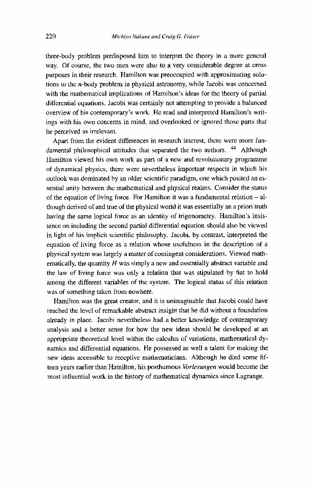
220 Michiyo Nakane and Cruig G. Fraser

three-body problem predisposed him to interpret the theory in a more general way. Of course, the two men were also to a very considerable degree at cross purposes in their research. Hamilton was preoccupied with approximating solutions to the n-body problem in physical astronomy, while Jacobi was concerned with the mathematical implications of Hamilton’s ideas for the theory of partial differential equations. Jacobi was certainly not attempting to provide a balanced overview of his contemporary’s work. He read and interpreted Hamilton’s writings with his own concerns in mind, and overlooked or ignored those parts that he perceived as irrelevant.

Apart from the evident differences in research interest, there were more fundamental philosophical attitudes that separated the two authors. Although Hamilton viewed his own work as part of a new and revolutionary programme of dynamical physics, there were nevertheless important respects in which his outlook was dominated by an older scientific paradigm, one which posited an essential unity between the mathematical and physical realms. Consider the status of the equation of living force. For Hamilton it was a fundamental relation - although derived of and true of the physical world it was essentially an a priori truth having the same logical force as an identity of trigonometry. Hamilton’s insis- tence on including the second partial differential equation should also be viewed in light of his implicit scientific philosophy. Jacobi, by contrast, interpreted the equation of living force as a relation whose usefulness in the description of a physical system was largely a matter of contingent considerations. Viewed math- ematically, the quantity H was simply a new and essentially abstract variable and the law of living force was only a relation that was stipulated by fiat to hold among the different variables of the system, The logical status of this relation was of something taken from nowhere.

Hamilton was the great creator, and it is unimaginable that Jacobi could have reached the level of remarkable abstract insight that he did without a foundation already in place. Jacobi nevertheless had a better knowledge of contemporary analysis and a better sense for how the new ideas should be developed at an appropriate theoretical level within the calculus of variations, mathematical dynamics and differential equations. He possessed as well a talent for making the new ideas accessible to receptive mathematicians. Although he died some fif- teen years earlier than Hamilton, his posthumous Vorlesungen would become the most influential work in the history of mathematical dynamics since Lagrange.

The Early History of Hamilton-Jacobi Dynamics 22 I

NOTES

1. The core of this article originated in the first author’s paper “C. G. Jacobi’s Discovery of a New Integral and his Extension of W. R. Hamilton’s Principal Function in Dynamics.” Parts of this paper were presented under the title “Some Aspects of Mathematization in the Construction of Hamilton-Jacobi Theory” at a joint meeting of the Canadian Society for History and Philosophy of Mathematics and the British Society for the History of Math- ematics, held in July 1999 at Victoria College of the University of Toronto. The authors would like to thank the participants at the joint meeting for discussions that were helpful in the preparation of this article. The comments of an anonymous referee are gratefully acknowledged.

2. See Hankins (1980, Chapters 2 and 4). 3. Nakane ( 1 991) discusses the three-body problem in Hamilton’s early dynamical work, em-

phasizing the role played by this problem in his formulation of the concept of the characteristic function.

4. See Kargon ( 1 965). In a letter to Samuel Coleridge in 1832 Hamilton wrote: “The atomistic theory of which I speak is nearly that of Boscovich, and consists in representing all phe- nomena of motion as produced by the action of’ localized energies of attraction or repulsion, each energy having a centre in space.. . ” (Kargon 1965, p. 138).

5. Compare Hamilton’s remarks with the following comments of Poisson: “ They [questions in mechanics] had to be treated in an entirely abstract manner.. .within this class of generality and of abstraction, Lagrange has gone as far as one could conceive possible when he replaced the physical connections [liens physiques] of bodies by the equations relating the coordinates of their different points. It is that which constitutes the analytical mechanics; but next to this admirable conception one can now offer the physical mechanics.. .” (Pois- son’s comments appeared in a memoir on elasticity from 1829 and are quoted by D. Arnold (1978, p. 254).) Although Poisson’s molecular programme must certainly be distinguished from Boscovich’s dynamism (as interpreted by Hamilton), there were significant similar- ities between the two conceptions. Hamilton had read Poisson’s writings, and Poisson’s physical mechanics would have been consistent with Hamilton’s understanding of dynamics. For more on Poisson, molecular physics and physical mechanics see (D. Arnold 1978, 1983).

6. See Hamilton’s remarks “To those imaginable cases. . . ” quoted in 5 2.3. 7. Lagrange, Hamilton and Jacobi used the notation ’ for differentiation with respect to time.

In our account we use the standard dot-notation of modem analytical dynamics. 8. Hamilton’s original form is U = Cmm,f(r ) . 9. Hamilton did not give the complete derivation. In particular, we have added equations

(2.1.10) and (2.1.12) following Hankins’s (1980,pp. 184-186) account. 10. Hamilton wrote for the partial derivative of V with respect to x,. 11. See Bolza (1906). Fraser (1999) refers to Hamilton’s dynamics and the field concept from

the viewpoint of the history of the calculus of variations. See Thiele (1997) for a history of field theory in the calculus of variations.

12. Consider the following example. A particle of unit mass moves under the action of no force in the plane from the origin to the point ( a , b ) . We posit that the trajectory is the straight line y = $x from 0 to ( a , b). For such a motion, we have the equation of energy v2 = 2H, or v = 2 = m. Hence the time of transit t is related to the total distance s = d m by equation s = r&%. Consider now a comparison trajectory ( f ( t ) , j ( t ) ) for which 6t = 6 H = 0. The particle can be made to traverse such a trajectory under the condition 6H = 0 by the introduction of suitable frictionless constraints. Since 6 H = 0 we have .? +? = H or 2 = 2H, or S = a . t * , where t* is the time of transit and 5 is the total path-length. Because 6 t = 0 we have t = t * . Hence 9= J 2 H . r = s = d m . This implies that ( f ( t ) , j ( t ) ) coincides with the straight line y = sx. The class of comparison curves has only one member: the line


y = gx itself. 13. For an account of Lagrange and the principle of least action see (Fraser 1983). A com-

prehensive study of variational principles in the eighteenth century is contained in (Puke 1989).

14. In (2.1.21a) V is a function o fy and H , V = V(y,H). To integrate this equation, we set H = constant. (2.1.2la) then reduces to an ordinary differential equation and may be integrated immediately using the condition V(b, H ) = 0 to produce (2.1.22). Similar remarks apply to (2.1.21b), with b substituted fory.

15. Hamiltonusedxll,all,yll, insteadofx,a,y,etc. and Hi and HI1 insteadofH1 and H2. 16. Conway and McConnell’s own support of this hypothesis may have wavered - see the

17. Demidov (1982, p. 331) describes Lagrange’s introduction of these concepts. 18. Hankins (1980, p. 23) notes that Hamilton mastered some textbooks written for the h o l e

Polytechnique, including Lagrange’s Thiorie des Fonctions analytiques. In a letter to H. F. C . Logan dated June 27, 1834 Hamilton wrote: “Your list of foreign books is very tantalising, but I shall only select the following, namely, Dircksen’s [sic] Griissten und Kle- insten and Pfaff and Cauchy on the Integration of Partial Differential Equations of thejirst Order, and these I would gladly purchase on the terms you mention.” (Graves V.2 1885, pp. 86-87). Although Hamilton had the opportunity, he does not seem to have become ac- quainted with contemporary theory of partial differential equations. Jacobi (1837, p. 11 1) suggested Hamilton’s inclusion of the second partial differential equation prevented him from taking notice of Lagrange’s results in the L e p n s sur le Calcul des Fonctions.

discussion at the end of this section.

19. See 2.5, equations (2.5.27) and (2.5.32). 20. Hamilton derived Lagrange’s equations as follows. From equation (2.1.1)

where

and

Hence we arrive at Lagrange’s equation. 21. For more discussion of variational principles see § 4.1. 22. In what follows the notation F‘(x) is used to designate $. 23. He also derived expressions for the mi, which we omit. 24. We have omitted the corresponding equations for mi. 25. The following comment of Dugas (1955, pp. 400-401) is relevant here: “Hamilton’s prin-

cipal function “would solve” the problems of dynamics. But, as a general rule, it could only be hoped to find this function by successive approximations. It is for this reason that Hamilton devoted so much effort to that task.”

26. Jacobi’s letter of 2 July 1830 was published in Borchardt’s Journalfir die reine und ange- wandre Mathemutik 80 (1875). pp. 271-3. In it the twenty-five-year old Jacobi’s writes: “le but unique de la science, c’est l’honneur de l’esprit humain, et que sous ce titre, une question des nombres vaut autant qu’une question du systkme du monde.” A few lines


later he reports: “J’ai rtfltchi aussi de temps en temps sur une mkthode nouvelle de traiter les perturbations ctlestes dans laquelle doivent entrer les thtories nouvelles des Functions Elliptiques.”

27. References to the work of Hill and Darwin are given by Moulton on p. 281. Jacobi’s integral is also derived by Edward John Routh (1898, pp. 154-155). The derivations of Routh and Moulton make use of rotating coordinate systems in which the coordinates of the comet are given in reference to a rotating coordinate system aligned along the line joining the two primary bodies. Jacobi’s derivation as we have reconstructed it was of a quite different sort.

28. Note that if % = 0 then we obtain just this principle, precisely as Lagrange (1788, pp. 202-205) himself had derived it in the Michanique Analitique.

29. Some examples of time-dependent potentials are given in (Wells 1967, pp. 90-91), a book in the “Schaum’s Outline Series in Engineering” whose intended audience is said to include “practising scientists and engineers.” Consider the following example: “Suppose that the string to which a pendulum bob is attached passes through a small hole in the support. Imagine the string pulled up through the hole with constant speed v.” If r is the length of the pendulum and ro is its intitial value then the potential V is given in the form V = -mg(ro - vt) cos 8.

30. Jacobi used the symbol a’ instead of 6. 3 1 . A very clear exposition of the modem derivation is contained in (Gelfand and Fomin,1963,

32. In his 184748 lectures Jacobi (1996, p. 189, p. 213) referred to the “symbolic equation” pp. 89-90). The endpoint formula is introduced on pp. 54-59.

6 ( T + U ) d t = O . S The equation was presumably merely “symbolic” because the quantity T + U has no clear physical or conceptual meaning. He attributed the equation to Hamilton, but noted that it is valid even when the forces and potentials contain the time. (In 1847-48, Jacobi explicitly used the modem term “Potenziel.”)

33. In the Vorlesungen (lesson 6, p. 44) Jacobi was critical of contemporary formulations of the principle of least action. In his Berlin lectures he (1996, p. 159) stated that Lagrange in his 1762 Turin memoir had formulated the principle in analytical mechanics in “a very unsystematic way.” Jacobi adhered in lesson 6 to the Eulerian formulation of the principle whereby the variable time is eliminated from the integrand by means of the equation of liv-

ing force. This principle is expressed by Jacobi in the form 6 1 -dm = 0. 34. In some modem textbooks on mechanics the term “Jacobi’s theorem” refers to a different

result, to the effect that a generating function for a canonical transformation is given by a solution to the associated Hamilton-Jacobi equation. See, for example, (Arnold 1989, p. 260). This convention seems to have originated with Poincart’s Les Mithodes Nouvelles de la Michanique Cileste, vol. 1 (1892). Although the result in question offers a way of solving the equations of motion, it is very different from the idea of Jacobi’s 1837 “ h e r die Reduction.” The latter showed how to reduce the equations of motion to a partial differential equation, but did not contain the idea of a canonical transformation.

35. It should be noted that in the twentieth Vorlesung Jacobi formulated the theorem in the setting where the integrand is of a general mathematical form.

36. See our account at the end of 0 2.3. 37. Consideration of this subject is beyond the scope of the present paper. For an overview and

assessment of Jacob’s contributions to the theory of first-order partial differential equations see (Demidov 1982, pp. 336-340) and (Hawkins 1991, pp. 200-217).

38. In 1848 Jacobi (1996, pp. 246-250) introducedcanonicalcoordinates and set p1 = = r,

p2 = 39. Hankins (1980, p. 196) in a natural attempt to reconcile this oddity in Hamilton’s theory,

actually replaces t by to in (2.4.19b). Conway and McConnell, in their commentary on

= ~ Z Q , p3 = $$ = rZsin’rpljl.


Hamilton, generally substitute to for Hamilton’s 0. As we shall see shortly, Jacobi in the nineteenth Vorlesung introduces the initial variable 7 in discussing Hamilton’s second equation. However, Hamilton himself is quite clear: the integration begins at 0, a real number and not a variable, and the partial derivative of S in the second equation is taken with respect tot , the same variable that it is taken with respect to in the first equation.

40. A partial English translation (via the French) of the relevant part of the Vorlesungen is provided in (Dugas 1955, pp. 401-403).

41. Hamilton’s actual response and his defense by Cayley are described by Hankins (1980, pp. 198).

42. Equation (4.3.1) is simply the standard endpoint formula for a field of extremals. Note that the use of the endpoint formula, rather than the procedure followed by Hamilton and Jacobi, considerably facilitates the derivation of the second partial differential equation (4.3.3). As we observed above, Hamilton and Jacobi would have had to reproduce the whole derivation of the Hamilton-Jacobi equation using 7-derivatives in order to obtain (4.3.3). (For the difference between the procedure of Hamilton and Jacobi and the modem approach involving the endpoint formu a see our discussion in 0 4.1 immediately following equation (4.1.12).)

43. In the calculus of variations the problem in which both endpoints are allowed to vary en- tails fairly general and fundamental considerations concerning the existence of fields of extremals. This problem, which is clearly beyond the scope of Hamilton’s dynamical analysis, is discussed by Bliss (1946, Chapter 2) in his account of sufficient conditions.

44. Puke (Jacobi 1996, pp. xxxix-lv) discusses ways in which Jacobi’s mechanics broke with earlier tradition in the exact sciences and anticipated some later themes in the philosophy of physics. The conventionalism that Puke identifies in Jacobi’s thought is consistent with our own account of Jacobi’s dynamics from the 1830s.

BIBLIOGRAPHY

Arnold, David H. 1987: “The MCchanique physique of SimCon Denis Poisson: The Evolution and Isolation in

France of his Approach to Physical Theory,” University of Toronto Ph.D. dissertation. 1983: “The MCchanique physique of SimCon Denis Poisson: The Evolution and Isolation

in France of his Approach to Physical Theory,” Archive for History of Exact Sciences 28, pp. 243-367.

Arnold, Vladimir I. 1989: Mathematical Methods of Classical Mechanics, (Second edition), Springer-Verlag,

New York. Bliss, Gilbert

1946: Lectures on the Calculus of Variations, Chicago. Bolza, Oskar

1906: “Weierstrass’ Theorem and Kneser’s Theorem on Transversals for the Most General Case of an Extremum of a Simple Definite Integral,” Transactions of the American Mathematical Society 7, pp. 459438.

Cayley, Arthur 1857: “Report on the Recent Progress of Theoretical Dynamics,” Report of the British As-

sociation for the Advancement of Science, pp. 1-42. 1862: “Report on the Progress of the Solution of Certain Special Problems of Dynamics,”

Report of the British Association for the Advancement of Science, pp. 184-252 = Mathematical Papers 4, pp. 513-593.

1889-1898: The Collected Mathematical Papers of Arthur Cayley, Arthur Cayley and An- drew R. Forsyth eds., 14 vols. Cambrige:At the University Press.

Conway, A. W. and McConnell, Albert J. 1940: “On the Determination of Hamilton’s Principal Function,” The Mathematical Papers

of Sir William Rowan Hamilton 2, pp. 613-621.


Dernidov, Sergey 1982: “The Study of Partial Differential Equations of the First Order in the 18th and 19th

Centuries,” Archive for History of Exact Sciences 26, pp. 325-350.

1852: “Gedachtnissrede auf Carl Gustav Jacob Jacobi,” Abhandlungen der Kiiniglichen Aka- demie der Wissenschaften zu Berlin aus dem Jahre 1852, pp. 225-252 = Jacobi’s Werke 1, pp. 3-28.

Dirichlet, Peter G. L.

Dugas, Rent

Fraser, Craig G. 1955: A History of Mechanics, Neuchgtel, republished by Dover, New York in 1988.

1983: “J.L. Lagrange’s Early Contributions to the Principles and Methods of Mechanics,” Archive for History of Exact Sciences 28, pp. 197-241.

1999: “Die Genese der Variationsrechnung,” in Geschichte der Analysis, ed. Hans Niels Jahnke, pp. 449486, Spektrum Akademischer Verlag: Heidelberg, Berlin.

1963: Calculus of Variations, Prentice-Hall, Inc.,Englewood Cliffs, New Jersey.

1950: Classical Mechanics, Addison-Wesley, Reading, Massachusetts.

1980: A History of the Calculus of Variations from the 17th through the 19th Century,

Gelfand, Izrail M. and Fomin, Sergey V.

Goldstein, Herbert

Goldstine, Herman H.

Springer-Verlag, New York.

1885: Life of Sir William Rowan Hamilton, Including Selections from His Poems, Corre- spondence, and Miscellaneous Writings 2, DublidLondon.

Graves, Robert P.

Hamilton, William R. 1834a: “On a General Method in Dynamics,” Philosophical Transactions Part 2, pp. 247-

308 = Mathematical Papers 2, pp. 103- 16 1. 1834b: “On the Application to Dynamics of a General Mathematical Method Previously Ap-

plied to Optics ,” Report of the British Association for the Advancement of Science, pp. 513-518= MathematicalPapers 2,pp. 212-216. “Second Essay on a General Method in Dynamics,” Philosophical Transactions Part 1, pp. 95-144 =Mathematical Paper.? 2, pp. 162-211. The Mathematical Papers of Sir William Rowan Hamilton 2, “Dynamics,” A. W. Conway and A. J. McConnell eds., Cunningham Memoir no.14, Cambridge: At the University Press.

1835:

1940:

Hankins, Thomas L. 1980: Sir William Rowan Hamilton, The Johns Hopkins University Press, BaltimoreiLon-

don.

1991: “Jacobi and the Birth of Lie’s Theory of Groups,” Archive fo r History of Exact Sci- ences 42, pp. 187-278.

Ivory, James I83 1 a: “On the Equilibrium of Fluids, and the Figure of a Homogeneous Planet in a Fluid

State,” Philosophical Transactions, pp. 109-146. 183 1 b: “On the Theory of the Elliptic Transcendents,”fhilosophical Transactions, pp. 349-

378. 1832: “On the Theory of the Perturbation of the Planets,” Philosophical Transactions, pp.

Hawkins, Thomas

195-228. Jacobi, Carl G. J.

1834: “iiber die Figur des Gleichgewichts,” Annalen der Physik 33, pp. 229-233 = Werke 2, pp. 17-22.

1836a: “iiber ein neues Integral fur den Fall der drei Korper, wenn die Bahn des staren- den Planeten kreisfonnig angenommen und die Masse des gestorten vernachlassigt


wird,” Auszug aus einem Schreiben an die Akademie der Wissenschaften zu Berlin. Monatsbericht, Juli 1836, pp. 59-60.

1836b: “Sur le Mouvement d’un Point et sur un Cas particulier du Problem des trois Corps,” Lettre adresste B 1’Acadbmie des Sciences de Paris, Comptes Rendus, t.3, pp. 59-61 = Werke 4, pp. 37-38.

1837a: “Zur Theorie der Variations-Rechnung und der Differential-Gleichungen,” Journal fur die Reine und Angewandte Mathemutik 17, pp. 68-82 = Werke 4, pp. 39-55.

1837b: “Uber die Reduction der Integration der partiellen Differentialgleichungen erster Ordnung zwischen irgend einer Zahl Variabeln auf die Integration eines einzigen Systems gewohnlicher Differentialgleichungen,” Journal fur die Reine und Ange- wandte Mathematik 17, pp. 97-162 = Werke 4, pp. 57-127.

1866: Vorlesungen iiber Dynamik, A. Clebsch ed., Berlin, reprinted by Chelsea in 1969. 1881-1 891: C.G.J. Jacobi’s Cesammelte Werke, Karl Weierstrass ed. 8 vols, Berlin. 1996: Vorlesungen iiber analytische Mechanik: Berlin 1847/48, Helmut Pulte ed., Braun-

schweigmiesbaden. Kargon, Robert

1965: “William Rowan Hamilton and Boscovichean Atomism,” Journal for the History of Ideas 26, pp. 137-140.

Kline, Morris

Koenigsberger, Leo 1972: Mathematical Thought from Ancient to Modem Times, Oxford.

1904a: Carl Gustav Jacob Jucobi, Rede zu der von dem internationalen Mathematiker- Kongress in Heidelberg veranstalteten Feier der hundertsten Wiederkehr seines Ge- burtstages, gehalten am 9. August 1904.

1904b: Carl Gustav Jacob Jacobi, Festschrift zur Feier der hundertsten Wiederkehr seines Geburtstages, Leipzig.

Lagrange, Joseph L. 1762: “Application de la Mdthode exposCe dans le Mdmoire prCcedCnt ii la solution de dif-

ferents problems de Dynamique,” Miscellanea Philosophica-Mathemutica Societatis Privatae Taurinensis, 2 = Guvres 1, pp. 363-468.

1772: “Essai sur le Probleme des trois Corps,” Prix de 1’AcadCmie Royale des Sciences de Pans, tome IX, 1772 = Guvres 6, pp. 229-33 1.

1774: “Sur 1’IntCgration des &pations B Diffkrences partielles du premier Ordre”, Nou- veaux Mdmoires de 1’Acade‘mie Royale des Sciences et des Belles-Lettres de Berlin, pp. 353-372 = Guvres 3, pp. 549-575.

1776: “Sur les IntCgrales pariculieres des Equations differentielles” Nouveaux Mdmoires de 1’Acaddmie Royale des Sciences et des Belles-Lettres de Berlin, pp. 197-275 = Euvres 4, pp. 5-108.

1788: Mdchunique analitique, Paris. Second edition, Mdchanique analytique vol. 1 (181 1) and v01.2 (1815), is reproduced in Guvres = Guvres 11, 12.

1197: The‘orie des Fonctions analytiques, Paris = (Euvres 9. 1806: LeFons sur le Calcul des Fonctions, Paris = Guvres 10. 1867-1892: Guvres de Lugrange, A. Serret and G. Darboux eds. 14 vols. Paris.

1970: The Variational Principles of Mechanics. Fourth edition. The first edition was published in 1949. University of Toronto Press.

Lancosz, Cornelius

Louville, Joseph 1856: “MCmoire sur un Cas particulier du ProblBme des trois Corps,” Journal des Math6

matiquespures et app1iquLe.s 1 (2 ser.), pp. 248-256. Lutzen, Jesper

1990: Joseph Liouville 1809-1882, Springer-Verlag, New York. 1995: “Interactions between Mechanics and Differential Geometry in the 19th Century”,

Archive for History of Exact Sciences, 49, pp. 1-72.


Moulton, Forest R.

Nakane, Michiyo 1914: An Introduction to Celestial Mechanics, New York.

1991: “The Role of Three-Body Problem in Construction of Characteristic Function for Me- chanics by w. R. Hamilton,” Historia Scientiarum, second series 1, pp. 27-38.

1892: Les Mithodes Nouvelles de la Mfchanique CPleste, vol. 1, Paris.

1809: “MCmoire sur la Variation des Constantes arbitraires dans les Questions de la Mtcha- nique,” Journal de l’kcole Polytechnique, 8 (15 cahier), pp. 266344.

PoincarC, Henri

Poisson, SimCon D.

Pulte, Helmut 1989: Das Prinzip der kleinsten Wirkung und die Krafrkonzeptionen der rationalen Mecha-

nik, Stuttgart. Routh, Edward J.

Scriba, Christoph J. 1898: A Treatise on Dynamics of a Particle, Cambridge.

1973: “JACOBI, Carl Gustav Jacob,” Dictionary of Scientijic Biography 7, pp. 50-55. C. C. Gillispie (ed.), Charles Scribner’s Sons. New York.

Thiele, Riidiger 1997: “On Some Contributions to Field Theory in the Calculus of Variations from Beltrami

to Hilbert,” Historia Mathematica 24, pp. 281-300.

1896: Traite‘de Michanique cfleste 4, Paris.

1967: Schaum’s Outline of Theories and Problems of Lagrangian Dynamics, McGraw-Hill,

Tisserand, Franqois F.

Wells, Dare A.

New York. Whittaker, Edmund T.

1899: “Report on the Progress of the Solution of the Problem of Three Bodies”, Report of

1944: A Treatise on the Analytical Dynamics of Particles and Rigid Bodies, 4th Edition, the British Association for the Advancement of Science, pp. 12 1-159.

Dover, New York.

the early history of hamilton-jacobi dynamics 1834–1837homes.chass.utoronto.ca/~cfraser/hj.pdf ·...

Documents