the economics of household solid waste …infohouse.p2ric.org/ref/49/48030.pdfthe economics of...

The Economics of Household Solid Waste Generation and Disposal1

Center for Economics Research, Research Triangle Instirufe, Research Triangle Park, North Carolina 27709

AND

College of Management, North Carolina Srafe Uniilersity, Raleigh, North Carolina 27695

Received June 13, 1990; revised June 30, 1993

We develop a household production model of waste management that explicitly incorpo- rates many of the technical and behavioral elements 'germane 10 current regulatory and non-regulatory solid waste policy initiatives. Examination of first-order conditions shows the interaction among household preferences, these production options, and external prices and fees. A simplified simulation of our model illustrates these relationships. showing that household response elasticities can vary widely over common price ranges and that relatively large household welfare gains may be obtained by adopting curbside recycling and unit pricing programs. e Academic Press [nc.

Federal and state environmental and health agencies are finding that controlling remaining environmental residuals increasingly involves modification of household purchases and production practices. A case in point is the plethora of local, state, and Federal solid waste policy initiatives ranging from recycling programs and mandates, to consumer packaging legislation, to volume- and weight-based pricing programs [23, 241. The ability of these initiatives to engage households in efforts to reduce and modify the solid waste stream determines both their environmental effectiveness and their economic impact. Similarly, our ability as economists to model and characterize household responses conditions the success of economic impact measurement and policy evaluation.

In this paper we explore using household production models as a means of analyzing and evaluating the household component of a variety of waste management initiatives such as changes in financing of waste collection service, recycling requirements, and collection options offered. First we develop a theoretical model of household choice that is rich enough to reflect key purchase, processing, and disposal options facing households across the country today. We then analyze the general properties of this model. Finally, we examine numerical solutions to an operational version of the model calibrated using parameters suggested by available data and what we believe are at. least plausible assumptions about household waste generation and management.

he authors thank two anonymous reviewers and the associate editor for their very helpful comments on earlier drafts.

215 . 0095-0696/94 $6.011

Copyright iI: I W4 by Academic Press, Inc. All rights of reprnductinn in any form reserved.

MORRIS AND HOLTHAUSEN

2. BACKGROUND

Until very recently, there has been only a small literature on the role of household decision making in the economics of municipal solid waste (MSW) because waste collection and disposal service has most often been financed by property taxes or modest fixed fees.* Studies of the price and income effects on solid waste collection and disposal services were initiated with the advent of environmental concerns about open landfills and increasing cost of alternative disposal methods in the 1970s. Using cross-section data, McFarland [12] estimated price and income elasticities for waste collection. He estimated a small, positive income elasticity of demand for waste collection (0.178) and an inelastic price elasticity of demand based on differences in f i e d fees (0.455)."

McFarland's estimate of the "price' elasticity of solid waste collection services was not accepted uncritically and subsequenf studies produced a wide range of price elasticity estimate^.^ This suggests that the context, including the availability and cost of alternative disposal options, is important to community response to changes in price and the estimation of any welfare effects associated with changing conditions of service and price. With the notable exception of Wertz [27], however, early studies did not integrate such considerations into their models.

In the more comprehensive model of household waste management developed here we include monetary incentives, in the form of unit prices, and alternate waste management technologies, in the form of waste reduction and recycling." '

3. A MODEL OF HOUSEHOLD MSW DECISION MAKING

We consider a utility-maximizing model of household behavior that is derived from a general household production model in which the household maximizes

'~ifferentials in the conditions of service have, however, provided the basis for some empirical research. For example, Hirsch [81 and Quon ef al. [I51 studied the effect of frequency of service on waste collected.

30ther estimates of income elasticity for MSW collection were made in the 1970s and, while the estimates vary by a factor of almost four. all show waste collection services to be a normal good. These estimates of income elasticity include the following: EPA (1973 [?I]). 0.404; Wertz (1976 [27]), 0.27-0.28; Downing (1075 [3]), 0.39; Tolley rt al. (1978 [20]), 0.3-0.7; Eflaw and Lanen (1979 [4]), 0.2-0.4.

' ~ o d d a r d [7], using McFarland's data, estimated a range from 0.33 to 0.77; Wertz [27] argued that the price elasticity was in the neighborhood of 0.15, while Eflaw and Lanen [4] concluded that the price elasticity was "highly inelastic" if not perhaps zero or even negative in sign. In Savas [16], data were presented that "show that those who pay variable fees are about as likely to generate (relatively) little refuse as those who pay by tax or flat fee."

'other recent research in this spirit includes Jenkins (91, who develops and estimates a model with a recycling option, and Morris and Byrd (131, who consider recycling and reduced "waste generation" as part of three community case studies on the effects of unit pricing on residential solid waste flows and costs of service.

waste reduction is defined as using household resources to limit the amount of waste generated as a by-product of household production of consumption goods. Households can d o this by changing purchases to reduce packaging and other excess material (e.g., buying products in economy sizes or those products with small amounts of packaging), or by using production techniques that employ by-products of consumption (e.g., re-use of jars, boxes, o r bags that originally contained purchased materials and use of re-usable production equipment such as durable knives, forks, and spoons).

ECONOMICS O F HOUSEHOLD SOLID WASTE 21 7

utility subject to production, time, and budget constraints.' This model is formu- lated as

max U ( X , L, R ) Y , H, L

( 1 )

Q( Y , H , X, W, R) = 0 (2) T = B + H + L (3)

w B = pY + c ( W - R) - CS,R, + F , i

(4)

where the variables are defined as

X A vector of goods produced and consumed by the household, X = ( x , , . . . , x, ) Y A vector of goods purchased by the household, Y = ( y , , . . . , y , ) T Total time available per period (e.g., per day) L Amount of leisure time per period H Amount of time spent in household production activities per period B Amount of time (e.g., hours) spent per period in market activities earning a

wage of w per hour w The hourly wage W Amount of waste material produced as a by-product of household production R Total amount of recycled material R, Amount of recycled material associated with production of x , Q The household's production function in which Y and H are inputs, and X, W,

and R are the joint outputs p A vector of prices for the purchased goods, p = ( p , , . . . , p,) c The cost per unit for waste collection

s, The credit (price) per unit of recycled waste produced along with good i production

F A fixed fee for waste collection.

This model is quite general and allows for a great deal of jointness in the production of consumption goods along with the generation, recycling, and disposal of waste. We restrict this model in two ways in order to make the model tractable but still capable of illustrating key relationships among consumption, waste reduction, recycling, and conventional disposal? First, we restrict the various household production functions by specifying separate production functions for the production of the consumption goods X, the amount of waste generated W, the amount recycled R, and the amount conventionally disposed G. This reduces the degree of jointness of the problem and expedites measurement of the amount

7 ~ u r t h e r generalization of the model is possible. For example, other arguments such as waste reduction may be added to the utility function, the time budget may be further subdivided, and a greater variety of waste management options included (e.g.. self-disposal by incineration). Such elaborations illustrate the many complicating elements that may enter the household's waste management calculations, but they do not alter the fundamental relationships identified in this analysis. The incorporation of such additional elements follows the pattern estahlished for the waste management options already represented in the model. We analyze a restricted but still informative version of the general model.

'conventional disposal here means conventional collection and disposal of mixed waste, typically by setting the material out for collection and ultimate disposal in a landfill o r by large-scale incineration.

218 MORRIS AND HOLTHAUSEN

of "effort" expended on waste reduction, recycling, and conventional disposal in dollar equivalents.

Let the production function for consumption good i be

where Hi, is the amount of time spent producing x i (for consumption) with purchased inputs Y. Let the production function for conventional disposal of production by-products of good i be

G; = 4 - R; = g ; ( H i g , Y ) , ( 6 )

where H,, is the amount of time spent in conventional disposal of residual waste with some purchased inputs Y. This residual is equal to the difference between waste generated by xi production and consumption (after any waste reduction activities) and the amount of waste material processed for re~ycling.~

Let the total amount of waste produced as a by-product of producing good i be

where Hi, is the amount of time spent reducing the amount of waste generated as a result of the production uf a unit of x i . In particular, we assume that fi(O, 0) = 1 so that zi is the amount of waste generated per unit of good i if no waste reduction effort is made.

The household recycles an amount Ri of the waste, y., associated with production of good i . The recycling production function is

Ri = hi(Hjr, 5, Y ) , (8)

where Hi, is the amount of time the household spends in activities designed to recycle the generated waste Wi.

The household's time constraint becomes

Using these relationships, the budget constraint can be written as

where pk is the price for purchased good y k .

9 ~ n practice, features associated with these waste production processes may affect the functional forms and choices (e.g., the wastes may be composed of several materials each of which may be waste reduced, recycled, and disposed with different degrees of ease). While some of this variation can be reflected in each good's waste production functions, the model can be adapted to multiple waste production functions for each of the different materials associated with each good.

ECONOMICS OF HOUSEHOLD SOLID WASTE 219

A second restriction characterizes the production functions for consumption goods and conventional waste disposal as fixed proportion functions. Thus, the amount of good i produced is

where the Of are parameters of the production function. Similarly, the amount of conventional waste disposed is

It follows that the full cost of producing one unit of good i is

The price, pi, thus includes both the opportunity cost of the household's time and the cost of any purchased inputs that are used in the production of good i. Further, the cost of disposing of one unit of conventional waste from good i production is

Dividing the waste reduction function K. by the amount of good i produced gives the following per unit waste reduction function:

w, = y/x, = z,fi(H,,,, Y ) . (15)

Given the prices of the inputs Y and the opportunity cost of the household's time, w , there is a minimum cost for achieving any given level of w,. Denote the minimum cost as cr,, and note that this cost is made up of the opportunity cost of time spent on waste reduction activities, Hi,, plus the cost of any purchased inputs used in the waste reduction effort. This minimum cost is given by the cost function associated with the production function f,.

Solving for the inverse cost function gives w, as a function of a,:

A similar, but simpler, set of manipulations will yield the per unit recycling function,

where p, includes the opportunity cost of time spent in recycling, Hi, , plus the cost of any purchased inputs used in the recycling effort.

The household receives utility from goods consumed, from leisure time, and from the amount of waste recycled.


Letting m = wT, the household's budget constraint can be written as

The household problem is to maximize utility with respect to the choice of xis, ais, Pis, and L, (i.e., maximize Eq. (1) subject to Eq. (18)). The corresponding Lagrangian expression is

A= U(X , , . . . , x,, R , L ) + A - CS,(W, - ri)xi i

where A 2 0 is the Lagrange multiplier.

4. ANALYSIS OF THE MODEL

The first-order Kuhn-Tucker conditions for this constrained optimization are the following:

ECONOMlCS OF HOUSEHOLD SOLID WASTE

where

au au au a~ ari aw, u, = - = - . - . - . - U, E - = - . - . - ,

' '" da, aR at-, dwi aa, l p api aR dri ap,

This formulation permits the values of xi, a,, p,, and L to be positive or zero.

4.1. Substitution across Goods

From Eq. (20a), one obtains conventional results where prices explicitly include not only time and purchased inputs used in producing the goods but also any additional costs of time and purchases associated with conventional disposal, waste reduction, and recycling net of any recycling credits per unit of the good."

The introduction of recycled materials into the utility function in this model implies that goods can be purchased for both their utility in consumption and the opportunity they provide for recycling in its own right. In the specific case of a Cobb-Douglas utility function as shown in Eq. (211, the effect of a change in x , on utility .can be decomposed into the sum of two distinct effects, as shown in Eq. (22):

The first term on the right of Eq. (22) is the direct effect of the consumption of good j on utility. The second term on the right is the indirect effect of x j recycling on utility. This effect is proportional to the weight of residuals managed for recycling per unit of xi consumed. This second term encourages the consumption of goods with high residuals generation if some of that residual can be easily managed for recycling.

4.2. Household Waste Reduction Efforts

The equilibrium condition that determines the household's waste reduction effort is shown as Eq. (20b). To simplify notation, we define ria 3 riwwia and UR = aU/dR and expand and rewrite (20b) as Eq. (23).

here is a theoretical possibility that, in the case of an inferior good, an increase in c would result in an increase in the amount of the good purchased. We note, however, the elusiveness of Giffen goods generally and the fact that the changes in c would raise the effective price of all goods simultaneously, albeit in different degrees.


Assuming that the household does purchase some xi and that a; is positive, we can rewrite Eq. (23) as Eq. (241, an expression that depicts the household's equilibrium when balancing the marginal costs and benefits of changing the level of waste reduction effort.

The left side is the gain (marginal benefit), per unit of x , consumed, from waste reduction (i.e., from increasing a; by one dollar). This benefit depends on the productivity of the household's efforts to reduce residuals generated in consumption of x i and is directly proportional to c + 8,.11

Equation (24) shows three elements of marginal cost associated with the increased waste reduction effort. The first term is the direct cost of the household's waste reduction effort. The second term derives from the fact that waste reduction makes it more difficult for the household to produce recycled materials from the waste and is proportional to the sum of the cost of conventional waste disposal and the credit received for selling the recyclable residuals, all weighted by the change in recycling productivity associated with the waste reduction effort. The third term is the monetized loss in utility resulting from the greater effort required to produce recycled materials, also weighted by the change in the recyciing productivity.

In this model, households have an incentive for waste reduction when (c + 6,) is positive, but the impact is automatically offset to some degree when households have an easy recycling opportunity. The strength of this offsetting effect is thc r,, component of rim, a term which in equilibrium is less than one.

4.3. Hoctsehold Effort to Irzcrease Recycling

Equation (20c) can be rearranged to analyze the household's equilibrium level of recycling effort. If x, and P, are positive, we obtain Eq. (25):

The left side of this equation measures the gain (marginal benefit) associated with recycling effort and the right side measures the marginal cost of this effort. The individual terms of this equation can be interpreted in a manner analogous to those described in Eq. (24), except that these terms reflect marginal changes due to a unit change in recycling effort pi. Increases in c encourage additional recycling of all goods and increases in 6, and s, encourage additional recycling of good i.

"If waste reduction also provides utility directly to the household, the left side of Eq. (24) would include the term U,/A within the parentheses, where D = T,(z , - w , ) x , and UI, = aU/aD. Since this term is positive, the benefits of the waste reduction effort (a,) will increase, and more waste reduction will be pursued by the household than would be the case without direct utility generation by waste reduction.

ECONOMICS O F HOUSEHOLD SOLID WASTE 223

5. SIMULATION WITH SELECTED PARAMETERS

The analysis of the equilibrium conditions of the model of household waste management developed in this paper helps identify relationships that shape household behavior. They also illustrate the complexity of household waste management choices and show that effective formulation and evaluation of municipal solid waste policy depends on the analyst's ability to accurately represent the relationships identified above. As an initial step toward such representation, this section presents a simplified but operational model of household waste management in a two-good world. In order to do this, given available data, we must make a variety of limiting assumptions, the most important of which is that leisure time is fixed. Thus households are characterized as trading work time ( B ) with household production time ( H I in their choice of purchases and production activitie~. '~

5.1. Simulation Specification

To perform the simulation we selected functional forms that met the usual requirements of consumer theory and any special restrictions associated with the model. We specify a Stone-Geary utility function to represent household utility, thereby allowing non-homothetic expansion paths. We also generalize the expression by specifying that the utility derived from recycling can differ with the good from which the recycled material originates. Equation (26) shows the general form of the utility function employed:

u = ( x , -

Selected production functions conform to the general conditions specified by the model. An inverse exponential function shown in Eq. (27) characterizes waste generation.

As shown in Eq. (28), the production function selected for recyclable materials is exponential in recycling effort and proportional to the amount of residuals generated.

Other equations of the simulation specify the income constraint and various accounting and boundary conditions. For example, total waste recycled as a by-product of good i consumption is the product of the amount recycled per unit of good i and the amount of good i consumption. Similarly, efforts devoted to recycling and waste reduction must be positive for each good.

The simulation of this model was implemented on a personal computer using the non-linear optimization software, GINO, developed by Lindo Systems, Inc.

he practical importance of this restriction is difficult to assess. Much depends on the rigidity of work time requirements. If, however, the value of leisure time is, at the margin, roughly equal to work time, then small changes in time allocation, such as considered here for household production, will not produce very different results whether the time budget allows changes in leisure time, work time, or both.


GIN0 uses a generalized reduced gradient algorithm to search the solution space for an optimum [I I]. By varying tolerance conditions, starting values, and bounds, and by running and re-running the program with these different settings, we were able to calibrate and explore the solution space for the household waste management model developed here.

5.2. Calibrating the Simulation Model

We calibrate the model using data on household expenditures and waste flows in two periods. Period 1 represents conditions and outcomes of household production choice with a conventional waste collection and disposal system financed with a fixed fee. Period 2 represents conditions and outcomes when the household pays for waste management by volume or weight and receives curbside recycling service at no additional charge.

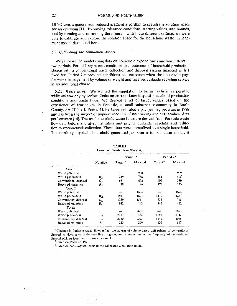
5.2.1. Waste flows. We wanted the simulation to be as realistic as possible while acknowledging serious limits on current knowledge of household production conditions and waste flows. We derived a set of target values based on the experience of households in Perkasie, a small suburban community in Bucks County, PA (Table I, Period 1). Perkasie instituted a pay-per-bag program in 1988 and has been the subject of popular accounts of unit pricing and case studies of its performance [14]. The total household waste flows are derived from Perkasie waste flow data before and after instituting unit pricing, curbside recycling, and reduction to once-a-week collection. These data were normalized to a single household. The resulting "typical" household generated just over a ton of material that it

TABLE l Houbehold Waste Flows (Ib/year)

-- -- -- -.- Per~od la Per~od 2"

Notat~on ~ d r g e t * Modeled ~ a r g e t ~ Modeled - -

Good l Waste potentlalC - 908 - 909 Waste generation % I 739 758 581 505 Conventional disposal G, I 661 672 407 330 Recycled materials R,I 78 86 174 175

Good 2 Waste potentialC - 1694 - 1694 Waste generation Yz 1501 1694 1179 1237 Conventional disposal G,2 1359 1551 733 745 Recycled materials Rtz 142 143 446 492

Totals Waste potentlalC - 2602 - 2603 Waste generation ? 2240 2452 1760 1742 Conventional disposal Gi 2020 2273 1140 1075 Recycled materials R, 220 229 620 667

-- - "Changes in Perkasie waste flows reflect the advent of volume-based unit pricing of conventional

disposal services, a curbside recycling program, and a reduction in the frequency of conventional d~sposal pickups from twice to once per week.

b ~ a s e d on Perkasie, PA. 'Based on consumption levels In the calibrated simulation model


needed to dispose of, most of which was set out for c~l lect ion. '~ After the concurrent introduction of unit pricing and curbside recycling (Table I, Period 2), the amount of waste generated dropped by about 20% and the amount recycled increased by nearly a factor of 3.". IS

We then allocated these residuals to two categories of household consumption, food and beverage consumption ( x , ) and all other consumption (x , ) , based roughly on the waste composition estimates provided in the Waste Plan model [SJ. These data indicated that roughly 33% of consumption residuals were food and beverage related and 67% were related to other household consumption: 739 Ib/year/household and 1501 Ib/year/household, respectively, before the unit pricing/recycling program. Because no commodity-specific waste data were available for Perkasie, we assumed that these proportions held after introducing unit pricing.'6 The amounts of recycled materials originating from the two goods were based on the composition of recycled materials reported by Perkasie; glass and aluminum were treated as originating from food and beverage commodities and paper from other commodities.

5.3. Time and Dolfar Budgets

We began deveIopment of budgets for the household using 1988 expenditure data for households in the fourth quintile of household incomes to estimate the share of household income allocated to the two goods [26]. This quintile had a median income that compared favorably with Perkasie: $30,967 vs $30,373 121. After allowing for taxes and under-reporting of expenditures, we calculated that out-of-pocket expenditures for the representative household were roughly $4137 on food and beverages and $23,160 on other goods.'7

These expenditures account, however, for only a 'portion of the household budget for consumption. In the model developed above, the household combines

13 There may be no indiiidual household that exhibits the waste flow patterns of Table 1. Indeed, the waste flows may even be uncharacteristic of individual households but, in as much as they represent aggregate effects, such considerations aren't critical to the validity of the simulation for calibrated conditions but may well be critical to using the simulated parameters to evaluate responses outside the "neighborhood" of calibrated conditions or policies targeted for specific types of households.

'?he initial waste flows of Perkasie are quite compatible with those cited by Franklin et al. [6] of residential waste generation for suburban communities of about 2.4 Ib/person/day. Multiplying the Franklin value by 2.83 persons/household in owner-occupied homes [24] and 365 days/year yields an estimate of waste generation of 2480 Ib/year/household compared to 2240 Ib/year for the typical Perkasie household used to calibrate this simulation.

15 In this simulation we attribute the difference between Period 1 and Period 2 waste generation to waste reduction. There are, however, other explanations for this change: burning, composting, deposit at second-hand stores, littering, inventory or storage, and sewerage, to name a few. Direct measures of these "diversionary" waste flows are not available. In general, communities contacted for EPA (251 did not believe that littering was a problem after offering recycling service with unit pricing. Aside from those observations and some anecdotal evidence, little is known for certain about the sources of interperiod waste flow changes or the specific waste reduction practices that are thought by many to be responsible for most of the observed change.

' h ~ y holding these proportions constant, we restrict the attractiveness in the calibrated model of differentially adjusting the waste reduction effort applied to the two goods and, in so doing, substitution across the two goods.

he data used in this simulation are represented with a precision that sometimes exceeds the accuracy of measurement. The small changes that occur in the model along with the exactness required to satisfy balance equations or identities necessitates this representation.


time with purchased inputs to produce the two commodities portrayed in this simulation. By assuming that the household has two "productive" members and estimating that 10,803 hours of their time are spent on leisure ( L ) , the balance of household time can be spent on income generation, (estimated to be 1864 hours) and household production (estimated as the residual or 4853 hours). The out-of- pocket expenditure and hour budget allow us to estimate an opportunity cost of time for the household (approximately $14.65/hour) and a total household budget denominated in dollars of $98,365.

To specify the "minimum consumption" parameters (?) of the Stone-Geary utility function, out-of-pocket expenditure data were obtained from the lowest quintile of the 1988 household expenditure survey [26]. Assuming that roughly 40% of household production effort on consumption is expended on food and beverages and 60% on other goods, we estimated $17,200 and $26,100 to be the minimum expenditures on purchased goods and household inputs for production of the two goods. This same assumption was later used to help choose initial targets for consumption levels in the first period. The basic premise was that the typical household devotes more time, relative to purchased inputs, producing food and beverages than it spends producing "other goods."

We also incorporated into the simulations fixed costs for the household production effort associated with waste handling (H,,) and recycling (H,,). This was done in part by introducing additional fixed costs into the income constraint. In particular, we assumed that the typical household spends a minimum of 20 minutes per week meeting waste handling requirements if any waste is to be conventionally disposed and a minimum of 14 minutes per week if any recycling is undertaken. Again using $14.65 as the marginal value of an hour, this amounts to incorporating fixed costs of $254 and $176 per year for waste handling and recycling, respectively." There is little empirical support for these values beyond our own experience and the comments of householders we've talked to about their waste management practices. The particular values selected have little influence on the solution other than to provide more plausible "total time" values for the simulation.

5.4. Calibration

Table II presents parameters of the calibrated simulation model. The "set" parameters are model parameters that are fixed and reflect either conditions in Perkasie, such as the type of waste financing, or conditions of the household derived from available data and assumptions as described above. The "calibrated" parameters were obtained by selecting values and running the simulation model iteratively until the results of household utility maximization approximated the target waste flows developed for the "typical" Perkasie household in Periods 1 and 2. More specifically, we first ran the model with set parameters that reflected a fixed fee condition and adjusted the calibrated parameters until target waste flow values were approximated. We then ran the model with set parameters that reflected unit pricing conditions and the set of calibrated parameters from Period

"The simulation might have included some fined costs for waste reduction as well, but such a modification would have required specifying values for which there exists even less empirical founda- tion, and which, as noted above, have no impact on the results.

ECONOMICS O F HOUSEHOLD SOLID WASTE

TABLE 11 Model Parameters Calibrated to Average Household Condit~ons

-- - -- . -- - - - Period 1" Period 2b

- -- - -- - Set parameters

Calibrated parameters

' ~ i x e d fee, drop-off recycling, twice-a-week collection of conventional waste. 'unit pricing, curbside recycling, once-a-week collection of conventional waste. '1n 1988 Perkasie charged $1.50 for a "40 Ib. bag," but the average weight of each bag was

approximately 20 Ib, thus the price parameter of $0.075/Ib.

1. The recycling parameters ( b , and b,) were then adjusted until the model's solution produced waste flows similar to those found in Period 2. We then fine tuned these results by sequentiaIly adjusting the calibrated parameters used in the Period 1 model, applying these parameters in the Period 2 version of the model, adjusting the parameters of that version of the model, and then starting the process all over again.

A particularly troublesome data element required by the model is the amount of waste that would be generated in the process of producing the consumption goods absent any waste reduction effort. We have no data on these parameters since we have no data on households that practice no waste reduction. When run with the final set of waste potential parameters z, and z2, the model produced Period 1 estimates of waste reduction of 6% all for good 1 (food and beverages).19 We

"we might have chosen to structure and calibrate the model assuming that no waste reduction occurred in Period 1. This would have freed us from estimating "waste generation potential" parameters zl and z2. We chose not to do this despite the weak basis for estimating these parameters because. it would have meant making equally uncertain adjustments in income to allow For the household's initial waste reduction effort. More importantly, since some households do undertake waste reduction efforts, we thought it provided for a richer and more stimulating characterization of household waste management to calibrate the model with a waste reduction component in Period 1.

228 MORRIS A N D HOLTHAUSEN

assumed that slightly more waste pcr unit was inherent in good 1 (food and beverages).

We based particular parameter adjustments on our understanding of the relationships among the parameters of the model and the waste flows that utility maximization would generate. We were guided by shadow prices computed for the various constraints and variables, but we had no formal search procedure for finding parameters that resulted in matching target values or a stopping rule to determine when we were close enough. The waste flows for the calibrated models finally obtained are shown in Table I. Those waste flow values are all within 15% of target values and most are within 10% for Period 1. A similar result obtains for Period 2: except for conventional waste disposal levels, which are about 19% below the target value, all differences are less than 15% and the majority are less than 10%.

5.5. Simulation Results

We used the resulting specification of the model to solve for utility-maximizing levels of household waste management under seven sets of conditions: the conditions of the two periods of calibration and five variations on those periods. The key variables for these sevcn scenarios are shown in Table 111. As noted above, F1 represents the fixed fee scenario in Period 1 without curbside recycling and with twice-a-week mixed waste collection. The simulations U12, U22, and U32 represent three different Period 2 unit pricing rates (1 = 0.05, 2 = 0.075, 3 = 0.10 $/lb) with curbside recycling and once-a-week collection. Other scenarios simulate the income reduction required to "compensate" the household for introducing the unit pricing program (HlU2) and the outcome of the model when a curbside recycling program is added to the fixed fee program (F2). We obtained these solutions by repeated use of the optimization software using model parameters developed from calibration of F1 and U22 while exploring different starting values, tolerances, and boundary condition^.^^

In F1, the household has no external or monetary incentive to reduce waste generation, only an "internal" incentive to reduce waste generation because of the marginal costs in time and purchased goods required to recycle or handle conventional disposal of the waste. The household also has a small "utility"-based incentive to recycle. The waste flows of F1 are reported in Table I as part of first-period calibration. Other values are reported in Table 111. Table I11 also shows the utility index under F1 (328.78) and variable household resource costs of waste disposal-approximately $135 for conventional waste disposal, $84 for

'O~on-linear optimization software is often finicky. Results obtained can vary not only with tolerances and starting points, but can also depend on the order and structure of equations, the accounting expressions introduced, etc. The GIN0 software automatically checks the duality of the solution to see if first-order conditions are satisfied, but failure to satisfy them in this application most likely reflects the computational limits occasioned by the wide range in model parameter values (loS to lo-'). One cannot guarantee that the second-order conditions have been satisfied or that the solutions represent a global optimum. What we did, and all we could do, was run these simulations under a wide variety of conditions, checking to see that no better, feasible solutions were found at boundaries or in the neighborhood of the solution selected as the optimum.

.%u!puno~ 01 anp sjelol 01 wns lou slied, .zzfl Uo!lelnru!s po!iad p u ~ aq] aierq!leo 01 pasn asoqi se u c ~ ! ~ e ~ n r u ~ s!ql JOJ awes aql ala sle!ia]eur papbar jo uo!]anpo~d uo slua!s!jjao3,

.pamnsuoD ? poo8 JO sa!l!luenb aqi dq nsos axnosal ploqasnoq alqerren %rr!p!n!p Lq pau!elqo aq dsur ('d pue ! x l ) %u!ls.bai purr uo!~anpa~ a1se.n JOJ s(ahaI . , IIoJ~~,, , .,

9LO I PLO 1 8LLI 806 LLOI OZE I PZZZ

9PL SPL O L l I 129 LPL € 2 6 I S S I

599 M P 999 68t PZ8 PZS H S Z I P L 9 9 06P 0 2 8 909 622 EP L

SOP ZOP 0 9LP ZOP R6Z 6 b l

E'EP t'9 1 S E P 5'9 1 9'OP 0-0 9 ' 0 S SZ Y 'EP P'9 I 9'EP P'S Y'ZE 0

S6'PZE ZP'8ZE SLO'O PZ'PZf 8L8ZE 5LO.O EP'PZE Et'6ZC 000'0 SP'PZf SC6ZC 001'0 ZS'PZE OS6Zf SLO'U PS'PZE 69'6ZE OSO'O 9 E ' M F 8L'82C 000'0

I x xaPu! (41/$) a ! l ! ~ n as!~d

v u n

ZnZH Z n I H

zsn zzn z1n

Id

(~raA/$) IQ ~ a ~ n o s a x ploqasnoH alqtyrrA -- . . -- . -- . - - . . . - . . -. .. . . .. - . - -. - - - - -- -. -

luaura%aue~ arsefi ploqasnoH Su!lelnw!s JO sllnsax III 318VL


TABLE IV Simulated Own- and Cross-Price Arc Elasticities

for Conventional Waste DisposalU

Price changes -

Elasticltiesb $0 0 to $0.$/lb $0.05 to $0.G5/lb $0.075 to SO.lO/lb - -- -

&X.C 0.15 0.51 0 60 & r , c 0.00 0.51 0.59 E z - w , c - 1.00 - 1.49 -0.97

"Arc elasticities calculated are based on simulations F1, U12, U22, and U32. h~ollowing convention, price elasticity is defined as the negative of the ratio percentage changes. A

positive elasticity value therefore represents an inverse relationship between price and quantity.

recycling, and $4 for waste reduction. Under U22, we eliminated the fixed fee and introduced unit pricing at 7.5 cents

per pound and curbside recycling service (reflected as a shift in the household's recycling production function).*' Again, model parameters were selected to assure that waste flows and fixed expenditures were approximately those target values based on Perkasie's experience in 1988. Under these conditions, the model produce a slightly higher utility index than that found in F1, indicating that the typical household was better off under unit pricing. Household annual variable resource costs for trash management were the following: $146 on conventional waste disposal (of which $81 was spent on purchasing bags for collection and disposal), $128 on recycling, and $28 on waste reduction. Total variable resource costs for waste management, after adjusting for the fixed fee, were $61 less in U22 compared to F1. If the price of bags did indeed cover the community's cost of the new waste management program (including curbside recycling), then the new system would be better for this representative household. This result is consistent with the generally favorable approval rating of Perkasie households reported by the town [I]. Comparing other aspects of solutions to F1 and U22 as shown in Table 111, we observe that consumption of both goods increased minutely with a corresponding increase in the household's "waste potential."

The simulation model allows us to isolate and examine solutions under different unit prices with curbside recycling in place over the range $0.00 to $0.10 per pound. The household responded by increasing waste reduction and reducing the amount of material recycled and conventionally disposed in response to increases in the unit price. Arc elasticities for these responses are displayed in Table IV. This particular simulation illustrates that price increases on conventional disposal don't necessarily result in increased recycling. In these simulations, the household found it more attractive to increase total waste reduction effort (from 13 to 40 dollars per year at the extreme price levels). The resources of time and purchased production inputs devoted to recycling were still high (there was actually a slight increase in recycling effort), but they were less effective because they were devoted

''AS noted above, the community that provides the waste flow data on which the calibration is based also switched to once-a-week service. We treat this change here as a shift in fixed costs from conventional waste disposal to recycling. In other words, from the household's perspective a curbside recycling collection day has simply been substituted for a conventional disposal collection day. This change, therefore, is assumed to have no effect on the household's waste management decisions beyond those noted above.

ECONOMICS OF HOUSEHOLD SOLID WASTE 23 1

to recycling materials from a waste stream diminished by waste reduction. The price increases resulted in a minute decline in household consumption of both goods.

The Hicksian compensation implied by H1U2 in this model was $117. In other words, to make the representative household no better off than it was before introducing unit pricing, curbside recycling, and once-a-week collection, annual income would have to be reduced by $117. This suggests that the joint unit pricing/curbside recycling program as simulated here results in substantial welfare improvements to the representative household.

We explore the welfare implications of the model further by simulating household waste management with curbside recycling (Period 2 recycling production function parameters) without changing the fixed fee (F2). In this scenario, no waste reduction effort at all was expended by the household and about $25 less effort was spent on recycling than in U22, but about the same amount was recycled. From the household's perspective, the Hicks compensation necessary to equate the utility derived from F2 and U22 is only.$l3 per year (H2U2).

While it.is tempting to conclude from these comparisons that nearly 90% of the welfare improvement stimulated by the Period 2 program was due to the advent of curbside recycling, this is not necessarily the'case. Recall that F1 and U22 were set up as programs that were roughly self-financing; in F2 the household produces much more recyclable material than that in F1 and 65% more conventional waste than U22.-It is highly likely that the community needs more than the $120 fixed fee to sustain the program of the F2 scenario, and this increased fixed fee will result in roughly a one for one increase in Hicksian compensation over the $13 calculated here. The exact size of the increase will depend on the collection and disposal cost functions for the recycling and conventional waste programs. If, as some observers contend, recycling is two or three times more expensive than conventional waste disposal, the fee increase could range from $30 to $60 per year and the contribu- tion of unit pricing to the welfare change from 30 to 50%.~*

The simulations also illustrate some of the problems that arise when recycling goals, however expressed, are combined with monetary incentives to reduce conventional waste generati~n. '~ When recycling mandates or goals are cast as a percentage of waste disposal service, attempts to reach that goal through monetary incentives to reduce conventional waste generation may be thwarted. The percentage of material recycled jumps from 9.34 to 38.25% because of introducing economic incentives to reduce conventional waste generation in combination with curbside recycling (F1 and U12). Comparing F2 and U12, we even observe that the unit pricing "component" of the change can account for a substantial share of this increase. However, simulations U12, U22, qnd U32 show that for the representa-

22 Another interesting possible link between household waste management and the conditions of service represented in simulation scenarios concerns littering or other unauthorized disposal. Should households select such disposal options to avoid paying for conventional disposal, additional costs incurred to control or remedy such behavior might have to be rolled into the price of service. Both of these examples illustrate the value of integrating household models such as that developed here into more general models that include the supply of waste management services to households.

22 This is not to argue that recycling services should be unit priced at zero but an acknowledgment that virtually all communities that apply unit pricing to conventional waste services do not charge a unit price for their recycling program.


tive household modeled here, the percentage of the easily measured waste stream (conventional waste plus recyclables) that is recycled drops very slightly as the price of conventional waste disposal increases. Because, at some price level, source reduction can begin to "dominate" household waste management, most of the reductions in conventional waste generation are due to source reduction, and the absolute amount of material actually recycled declines. This means that if the frame of reference is some past level of conventional and recycling service provided, say in Period I, the introduction of unit pricing of conventional waste service without change in the opportunity to recycle can actually reduce the percentage of material recycled (compare F2 with U12).

6. SUMMARY AND CONCLUSIONS

Using a household production model of household solid waste management, we show how broadening the characterization of a household's waste management options and the way in which those services are financed updates and clarifies the economics of household waste management and provides a better basis for assessing the impacts of policies for solid waste management. Some of the observations derived from the model are commonplace in economics but may otherwise be lost in the context of solid waste. For example, households' price of consumption already includes a waste management component whether haulers assess a unit charge for their services or not, and the effects of economic incentives aimed at encouraging source reduction and recycling will depend on the existence of purchased commodities and production opportunities that satisfy similar consumption requirements while generating very different amounts and types of residuals. Other observations derived from the model are. more thought provoking. In particular, the model highlighted the relationship between waste reduction and recycling and the fact that these management options were not merely alternate means of dealing with waste, but were linked technically in such a way that more of one had an adverse effect on the household's incentive -to use the other, This raises serious questions about the wisdom of the waste disposal "hierarchy" as a p o ~ mandate 122, 17A

In the second part of this paper, we implemented a simplified version of the household production model to both illustrate the properties of the model and stimulate thinking about the empirical requirements and initial results of such a simulation exercise. While we developed parameters for the simulation by calibrating the model to actual waste flows, prices, and expenditures observed in a small community under two very different economic and institutional regimes, many data elements required by even the simplified model either were not observable or were not available to us. For example, we had no observations on waste generation "potential" and only very primitive data on residual flows and their disposition by commodity. The data demands for even the simplest of such models are high and should properly be regarded as both a very difficult hurdle for implementation and a basis for caution regarding any particular results generated.

Recognizing such limitations, however, the development and use of the simulation in this paper made it possible to illustrate a number of important points. First, it provided initial estimates of household resources devoted to different waste management practices under alternative conditions of service and prices: tens of


dollars per year in variable household resource costs for disposal alternatives and probably under $200 per year in total. Second, simulation provided a means of estimating key price elasticities. For prices of conventional waste disposal service, the own price elasticity was inelastic but high by the standards of the literature (0.51 to 0.60), the cross-price elasticity with recycling was negative but less than one, and the cross-price elasticity with waste reduction was near one or higher. Third, it provided initial welfare estimates of changes in price and conditions of service, albeit in a partial equilibrium context for those simulations where collection and disposal costs would be affected. In the case of two periods used to calibrate the model, the initial estimate of Hicks' compensation required by the household to offset the benefits of a simultaneous change to unit pricing, curbside recycling, and once-a-week collection was a startling $117 per year. Finally, the simulation illustrated both the possible shortcomings of using economic incentives as a means of meeting ambitious recycling goals and the problems of setting sensible goals in the context of household waste management with linked, multiple disposal alternatives.

REFERENCES

1. L. Becker, "Annual Report of the Borough of Perkasie: Per Bag Disposal Fee, Waste Reduction, and Recycling Program," June (1991).

2. Bucks County Planning Commission, Perkesie borough comprehensive plan, Draft 1 (1989). 3. P. B. Downing, The distributional impact of user charges for refuse collection, Mimeo, Virginia

Polytechnic Institute and State University, Blacksburg, VA (1975). 4. F. Eflaw and W. N. Lanen, "lmpact of User Charges on Management of Household Solid Waste,"

Report prepared for the U.S. Environmental Protection Agency under Contract 68-03-2634, Mathtech, Inc., Princeton, NJ (1979).

5. Energy Systems Research Group, Inc., "Waste Plan-The Solid Waste Management Planning Tool: User Guide, Version 89-8," Boston, MA (1989).

6. W. A. Franklin, M. A. Franklin, and R. G. Hunt, "Waste Paper: The Future of a Resource 1980-2000," Prepared for the Solid Waste Council of the Paper Industry, Prairie Village, KS (1 982).

7. H. C. Goddard, "Managing Solid Waste," Praeger, New York 11975). 8. W. Hirsch, Cost functions of an urban government service: Refuse collection, Rev. Econ. Statist.

47, 87-92 (1965). 9. R. Jenkins, "Municipal Demand for Solid Waste Disposed Services: The lmpact of User Fees,"

Ph.D. Dissertation, University of Maryland (1991). 10. P. Kemper and J. M. Quigley. "The Economics of Refuse Collection." Ballinger, Cambridge, MA

(1976). 11. J. Liebman, L. Lasdon, L. Schrage. and A. Waren, "Modeling and Optimization with GINO."

Scientific Press, Pa10 Alto, CA (1986). 12. J . M. McFarland, .Economics of solid waste management, in "Comprehensive Studies of Solid

Waste Management, Final Report," Sanitary Engineering Research Laboratory, College of Engineering and School of Public Health, Report No. 72-3, pp. 41-106, University of California, Berkeley, CA (1972).

13. G. E. Morris and D. C. Byrd, The effects of weight- o r volume-based pricing on solid waste management, Draft report prepared for the U.S. Environmental Protection Agency, Research Triangle Institute, Research Triangle Park, NC (1990).

14. 8. Paul, Pollution solution-Pennsylvania town finds a way to get locals to recycle trash, WaN Slree! J. June 21, A-1 (1989).

15. J. Quon, M. Tanaka, and A. Charnes, Refuse quantities and frequency of service, I. Sanitary Eng. Dil,. 94, 403-420 (1968).

16. E. S. Savas, "The Organization and Efficiency of Solid Waste Collection," Lexington Books, Lexington, MA (1977).


17. J. Schall, "Does the Solid Waste Management Hierarchy Make Sense? A Technical Economic, and Environmental Justification of the Priority of Source Reduction and Recycling," Working Paper, Program on Solid Waste Policy, Yale University (1992).

18. K. A. Sproule and J. M. Cosulich, Higher recovery rates: The answer's in the bag, Resour. Recycling (Nov./Dec.), 20-21. 43-44 (1988).

19. B. J. Stevens, Scale, market structures, and the cost of refuse collection, Reo. Econ. Stathr. 60(3). 438-448 (1978).

20. G. S. Tolley, V. S. Hastings, and G. Rudzitis, "Economics of Municipal Solid Waste Management: The Chicago Case." EPA-600/8-78-013, U.S. Environmental Protection Agency, Cincinnati, OH (1978).

21. U.S. Environmental Protection Agency, "Socioecnomic Factors Affecting Demand for Municipal Collection of Household Refuse," Washington, DC (1973).

22. U.S. Environmental Protection Agency, "The Solid Waste Dilemma: An Agenda for Action," EPA/530-SW-88-054, Washington, DC (1988).

23. U.S. Environmental Protection Agency, Office of Air Quality Planning and Standards. "Economic Impact of Air Pollutant Emission Standards for New Municipal Waste Combustors." EPA- 450/3-89-006, Research Triangle Park, NC (1989).

24. U.S. Environmental Protection Agency, Office of Solid Waste, "The Solid Waste Dilemma: An Agenda for Action," EPA/530-SW-89-019, Washington, DC (1989).

25. U.S. Environmental Protection Agency, Office of Policy, Planning and Evaluation. "Guide to EPA's Unit Pricing Database: Pay as You Throw Municipal Solid Waste Programs in the U.S.," EPA/230-3-93-002, Washington, DC (1993).

26. U.S. Department of Commerce, Bureau of the Census, "Statistical Abstract of the United States," U.S. Government Printing Office, Washington, DC (1988).

27. K. L. Wertz, Economic factors influencing households' production of refuse, J . Enciron. Econ. Management 2 , 263-272 (1 976).

the economics of household solid waste …infohouse.p2ric.org/ref/49/48030.pdfthe economics of...

Documents