See discussions, stats, and author profiles for this publication at: https://www.researchgate.net/publication/324120471

The effect of design drift limit on the seismic performance of RC dual high‐

rise buildings

Article  in  The Structural Design of Tall and Special Buildings · March 2018

DOI: 10.1002/tal.1464

CITATIONS

6READS

1,396

3 authors:

Some of the authors of this publication are also working on these related projects:

Thesis 's paper View project

Seismic performance of tall buildings View project

Mohsen Zaker Esteghamati

Virginia Polytechnic Institute and State University

9 PUBLICATIONS   13 CITATIONS   

SEE PROFILE

Mehdi Banazadeh

Amirkabir University of Technology

46 PUBLICATIONS   233 CITATIONS   

SEE PROFILE

Qindan Huang

University of Akron

47 PUBLICATIONS   428 CITATIONS   

SEE PROFILE

All content following this page was uploaded by Mohsen Zaker Esteghamati on 18 February 2020.

The user has requested enhancement of the downloaded file.

Received: 14 April 2017 Revised: 22 August 2017 Accepted: 29 November 2017

DO

I: 10.1002/tal.1464

R E S E A R CH AR T I C L E

The effect of design drift limit on the seismic performance ofRC dual high‐rise buildings

Mohsen Zaker Esteghamati1,2 | Mehdi Banazadeh2 | Qindan Huang1

1Department of Civil Engineering, The

University of Akron, Akron, Ohio, USA

2Civil and Environmental Engineering

Department, Amirkabir University, Tehran, Iran

Correspondence

Mehdi Banazadeh, Associate Professor, Civil

and Environmental Engineering Department,

Amirkabir University, Room No. 409, Faculty

of Civil Engineering 424, Hafez Ave., PO Box

19648‐15914, Tehran, Iran.Email: mbanazadeh@aut.ac.ir

Struct Design Tall Spec Build. 2018;27:e1464.https://doi.org/10.1002/tal.1464

SummaryCurrent building codes aim to ensure the acceptable performance of structures implicitly.

Because these provisions are empirically developed for low‐ to medium‐rise buildings, their appli-

cability to high‐rise building warrants further investigation. In this paper, the effect of design drift

limit on the seismic performance of reinforced concrete dual high‐rise buildings is considered.

Nine buildings are designed for 3 drift limits: the code limit (i.e., 2%), one that is lower than the

code limit (i.e., 1.5%), and one that is higher than the code limit (i.e., 3%). For each drift limit, build-

ings of 3 heights (20, 25, and 30 stories) are designed. Finite element models are constructed in

OpenSees, and incremental dynamic analysis is performed. The results are used to develop prob-

abilistic seismic demand models, where model parameters are determined using maximum likeli-

hood estimation to incorporate equality and censored data. Reliability analysis using probabilistic

demand models is conducted to derive seismic fragility and demand hazard curves. In addition,

the collapse performance of the drift limits is evaluated using the Federal Emergency Manage-

ment Agency (FEMA) P695 procedure. The study results show that the design drift limit affects

the building's seismic performance, and the effect depends on the performance level considered.

Moreover, from a structural integrity perspective, a larger design drift limit does not induce a

significantly higher risk and might yield a more cost‐effective design.

KEYWORDS

design drift limit, high‐rise structures, incremental dynamic analysis, performance‐based earthquake

engineering, probabilistic models, reliability analysis

1 | INTRODUCTION

The minimum height of a structure to be considered as a high‐rise building varies from 10 stories to 60 m. The number of buildings with a height of

200 m or more has increased by 392% in the last 15 years. In 2015, 106 of these structures were completed, which was a new world record.[1] The

significant social and economic impacts of recent earthquakes[2,3] and the worldwide surge in high‐rise construction have drawn attention to the

challenges of the design and assessment of tall buildings.[4,5] Three major issues in the application of current building codes for the design of tall

buildings are

• The current codes do not explicitly quantify performance due to their empirical nature.

• Seismic design coefficients (e.g., response coefficient, R, and amplification factor, Cd) are used to relate elastic design to inelastic responses.

However, because these coefficients are primarily calibrated for low‐ to medium‐rise buildings based on engineering judgment,[6] they may

not be suitable for high‐rise buildings.

• Common codes are developed to provide design requirements for general structures rather than a specific class of structures. Therefore,

following the same design procedures could yield structures with different performance. For example, ASCE 7‐10 (and earlier versions)[7]

allows the same drift limits for high‐rise structures as for low‐ and medium‐rise ones.

Copyright © 2018 John Wiley & Sons, Ltd.wileyonlinelibrary.com/journal/tal 1 of 16

2 of 16 ZAKER ESTEGHAMATI ET AL.

The issues mentioned above motivate researchers to revisit tall building design using approaches that can consider the structural perfor-

mance directly. Performance‐based earthquake engineering (PBEE) is a probabilistic framework to assess performance using quantitative

metrics that consists of four components: hazard analysis, structural analysis, damage analysis, and loss analysis. In structural analysis, PBEE

implements probabilistic seismic demand models to estimate the seismic fragilities and/or mean annual frequency (MAF) of a structure exceed-

ing a given demand under a specific hazard level.[8,9] In PBEE, numerical models of structures are typically subjected to a suite of ground

motion records to conduct nonlinear response history analysis, and the structural responses are recorded in terms of engineering demand

parameter (EDP). Seismic fragility refers to the conditional probability of exceeding a limit state (usually described by a specific EDP and its

corresponding capacity) for a given seismic intensity measure (IM). The MAF is calculated by multiplying the IM hazard (i.e., the probability

of IM occurrence from the seismic hazard of the site) with the probability of EDP exceedance conditioned on the selected IM and integrating

over the entire range of the IM.[10,11]

Despite the wide attention given to the use of probabilistic seismic evaluation for code‐conforming low‐ to medium‐rise structures,[12–15] few

studies have focused on tall buildings. Haselton et al.[16] used the PBEE framework to evaluate the effect of the minimum base shear requirement

of ASCE 7‐05 and the strong‐column/weak‐beam concept of ACI 318 on the seismic performance of 30 reinforced concrete (RC) special moment‐

resisting frames (SMRFs) and suggested that mid‐rise structures are more likely to collapse than high‐rise ones. Jalali et al.[17] investigated the

seismic performance of 3‐, 7‐, and 15‐story steel moment frames with a generic locally reinforced connection. They showed that as structure height

increased, the MAF of collapse decreased. However, this trend reversed when the models were evaluated for the immediate occupancy limit state.

Asgarian et al.[18] studied a 30‐story steel structure with a framed tube system using PBEE to assess the impact of different IMs on the incremental

dynamic analysis (IDA) results. They showed that tall buildings have lower MAF at large drift levels compared to shorter steel frames. Mathiasson

and Miranda[19] evaluated the collapse probability of a 20‐story steel SMRF structure designed based on ASCE 7‐10 and showed that it met code

collapse performance. Sadraddin et al.[20] investigated the effect of shear wall configuration on the fragility assessment of a 12‐story RC high‐rise

structure and reported that adding shear wall improved the structural behavior under all the studied limit states. Pejovic and Jankovic[21] proposed

an analytical procedure to develop fragility curves for 20‐, 30‐, and 40‐story RC core‐wall high‐rise buildings, considering the threshold values for

the limit states as random variables correlated with damage indices.

Drift criteria govern the behavior of tall buildings under lateral load; thus, the design drift value determines the lateral resisting system

selection and material efficiency.[22] In addition, drift requirements are included in the codes to address structural integrity, nonstructural

component damage, and occupant comfort during vibration‐induced motions such as earthquakes or wind.[23] Therefore, there is a need to

better understand the relationship between the design drift limit and structural performance. On the other hand, based on the current litera-

ture, the suitability of design drift limits for tall buildings has not been evaluated to date. Therefore, this study aims to investigate how the

ASCE 7‐10 design drift limit affects the seismic performance of high‐rise structures from a structural integrity perspective. In particular, the

seismic performance of three configurations (i.e., 20‐, 25‐, and 30‐story) for conventionally designed RC high‐rise buildings with shear walls

is evaluated. For each configuration, three buildings are designed using different drift limit values. IDA is performed on the numerical models

of the prototype buildings. The performance of the structures is evaluated and compared in terms of seismic fragility, seismic demand hazard,

and adjusted collapse margin ratio (ACMR).

2 | PROTOTYPE BUILDING DESIGN

Shear wall–frame dual lateral resisting systems are quite popular in high‐rise building construction, as the interaction of frames and the shear

wall can reduce the lateral displacement for structures up to 70 stories.[24] Therefore, in this study, dual RC high‐rise structures are adopted

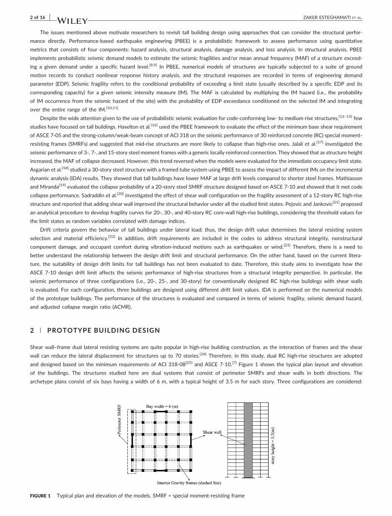
and designed based on the minimum requirements of ACI 318‐08[25] and ASCE 7‐10.[7] Figure 1 shows the typical plan layout and elevation

of the buildings. The structures studied here are dual systems that consist of perimeter SMRFs and shear walls in both directions. The

archetype plans consist of six bays having a width of 6 m, with a typical height of 3.5 m for each story. Three configurations are considered:

FIGURE 1 Typical plan and elevation of the models. SMRF = special moment‐resisting frame

ZAKER ESTEGHAMATI ET AL. 3 of 16

20‐, 25‐, and 30‐story. Because this study focuses on the global responses of structures, some common architectural practices for tall building

construction (such as podiums) are not considered in the modeling. Based on ASCE 7‐10,[7] the designed floor live load values of 1.96, 0.98,

and 1.47 kN/m2 are used for the floor, partition, and roof live loads, respectively. Floor slabs are modeled using membrane elements, providing

a loading transfer path and constraint to other structural members. Columns are assumed to be fixed at the base. The compressive strength of

concrete used in walls and frame components is assumed to be 55 MPa, and ASTM A615 rebar with a yield strength of 413 MPa is used as

the reinforcement.

The building site is assumed to be located in San Jose, California, with a latitude and longitude of 37.34°N and 121.89°W, respectively.

Based on the seismic design category D (high seismic vulnerability) with a risk category of I and a soil site classification of D (stiff soil), the

maximum considered earthquake (MCE) spectral acceleration at short periods (Ss), and 1‐s period (S1) are determined as 1.5 and 0.6 g, respec-

tively. In this study, the modal response spectrum analysis (ASCE 7‐10[7]) is selected for the tall building design. In the modal response

spectrum analysis, the structure is treated as a multidegree‐of‐freedom system associated with different modes. For each mode, the base shear

is calculated using the spectral acceleration of the design spectrum at the corresponding period multiplied by the mass of the system. The

structure base shear is then determined by a combination of responses from a sufficient number of modes, corresponding to at least 90%

of the effective mass. In this study, the first 11 modes are used in the design. Next, the base shear values calculated from the response

spectrum analysis are scaled to 85% of the base shear forces obtained from the equivalent lateral force analysis.[23] In the equivalent lateral

force, the response modification coefficient, R, and the deflection amplification factor, Cd, are taken as 7 and 5.5, respectively, for the dual

system. The SMRFs are designed to withstand 25% of the total seismic forces, whereas the combination of shear walls and frames resists

the total seismic forces, complying with the ASCE 7‐10 requirement for dual systems. The strong‐column/weak‐beam concept is considered

throughout the design phase.[25]

According to ASCE 7‐10,[7] the design drift limit (i.e., the maximum allowable drift) for dual buildings is 2%. To investigate the impact of this

code drift limit on the seismic performance, three buildings are designed for each configuration based on three drift limits: (a) an interstory drift

ratio of 1.5%, which is lower than the code limit; (b) an interstory drift ratio of 2%, corresponding to the code limit; and (c) an interstory drift ratio

of 3%, which is higher than the code limit. Thus, nine buildings are designed. A strict trial‐and‐error approach is used to ensure that the maximum

allowable drift ratio of each building does not exceed the corresponding design drift limit. Each building is named according to the number of

stories, n, and the design drift limit, m%, in the format nS/m%D. For example, the 20‐story building designed with a drift limit of 2% is denoted

as 20S/2%D.

Table 1 provides the summary of characteristics of the buildings. As shown inTable 1, for a given height, buildings designed for 1.5% drift limit

(i.e., the most strict drift limit) have the heaviest weights and the smallest modal periods. In addition, for a given height, the design base shear of the

1.5%D buildings are the largest, because they have the largest design spectrum acceleration and the greatest weight. Figure 2 shows the first three

modal shapes of a typical perimeter frame of building 20S/2%D, which are similar to other prototype buildings. Tables A1 and A2 show the

designed sections of frame members and shear walls, respectively, for the prototype buildings based on modal response analysis results. For frame

columns and beams as shown inTable A1, the buildings with a design drift limit of 1.5% have larger sections and more reinforcement, whereas the

buildings with a design drift limit of 3% have smaller sections and less reinforcement, as compared to the 2%D structures. In particular, Building

20S/1.5%D has beam sections that are up to 33.9% larger than 20S/2%, whereas Building 20S/3% reduces the column and beam sections up

to 40.8% and 35.9%, respectively. Similar findings are obtained for 25‐ and 30‐story buildings. As shown inTable A2, the 25‐ and 30‐story buildings

with a design limit of 1.5% have walls with larger thicknesses, whereas the 20‐ and 25‐story buildings with design limit of 3% have walls with

smaller thicknesses. Figure 3 shows the drift profiles of nine buildings obtained from the response spectrum analysis. As shown in Figure 3, all

the drift profiles are within the corresponding design drift limits.

TABLE 1 Building characteristics of the prototype buildings

Building

Modal periods (s)Weight(kN)

Design base shear(kN)1 2 3

20S/1.5%D 2.74 0.79 0.38 254775.37 11391.65

20S/2%D 3.18 0.86 0.39 236936.3 10455.13

20S/3%D 4.03 1.01 0.44 204527.36 9213.52

25S/1.5%D 3.36 1.03 0.51 333016.77 12791.61

25S/2%D 3.88 1.15 0.54 308499.57 11850.03

25S/3%D 4.66 1.34 0.61 273719.45 10567.37

30S/1.5%D 3.99 1.26 0.62 358221.11 13970.51

30S/2%D 4.46 1.45 0.70 329029.10 12673.45

30/3%D 5.85 1.67 0.79 285942.42 11347.61

FIGURE 2 Modal shapes (solid line) and undeformed shapes (dashed line) of the perimeter frame of a 20‐story model: (a) first mode (b) secondmodel, and (c) third mode

FIGURE 3 Drift profiles of the designed prototype buildings

4 of 16 ZAKER ESTEGHAMATI ET AL.

3 | NUMERICAL ANALYSIS

3.1 | Finite element models

Finite element models were constructed in OpenSees,[26] following the recommendations of the Applied Technology Council regarding the numer-

ical analysis of tall buildings.[27] The schematic in Figure 4 shows the configuration of the numerical model. As shown in Figure 4, the leaning column

is connected to the SMRF by rigid truss elements at the floor level and is pinned at the base. The seismic weight of the interior gravity system is

assigned to the leaning column. The P‐delta effects are thus considered through the leaning column. The shear walls are fixed at the base and are

connected to the SMRF by rigid links to consider shear wall–frame interactions. The slab effect is modeled as a rigid diaphragm to constrain all

nodes at each floor level.

In the SMRF, the beam–column joints are modeled using the joint2D element in OpenSees. As illustrated in Figure 4, this element creates a

parallelogram with a node at the center of the panel zone and four external nodes that connect the panel zone interfaces to the adjoining elements.

The central node has one extra degree of freedom to account for the shear deformation and is connected to the external nodes by kinematic

constraints.[28] The frame components (i.e., beams and columns) are modeled using a concentrated plastic hinge model that consists of an elastic

element with inelastic rotational springs at both ends. The elastic element is modeled using element ModElasticBeam2D in OpenSees, which refers

to an elastic beam column element with a stiffness modifier that is used to address damping and convergence problems associated with concen-

trated hinge models.[29]

The behavior of the inelastic rotational spring in the plastic hinge model is defined using the Ibarra–Krawinkler deterioration model,[30] where

both monotonic stiffness degrading and cyclic deterioration of stiffness and strength are included. The deterioration reflects the degree of damage

that a structural member experiences when responding to the loading. This becomes more critical when the structure undergoes large inelastic

deformations (such as those occurring in a near collapse state). The backbone curve of the inelastic rotational spring is defined using four quantities:

yielding moment, My; plastic hinge rotation capacity, θp; plastic hinge post‐capping rotation capacity, θpc; and effective stiffness, ke (as shown in

Figure 4). In the Ibarra–Krawinkler deterioration model, a strength deterioration parameter, λs, and a stiffness deterioration parameter, λe, are used

to capture the structural damage during cyclic loading in terms of strength and stiffness, respectively. In this study, θp, θpc, λs, and λe are derived

FIGURE 4 Configuration of nonlinear models

ZAKER ESTEGHAMATI ET AL. 5 of 16

from the regression equations developed by Haselton et al.,[31] whereas My is determined based on equations from Panagiotakos et al.[32] It is

worth noting that θpc is also restricted by the upper bound of 0.1, as suggested by the PEER/ATC 72‐1.[27] Also, based on the equations by

Haselton et al.,[31] the effective stiffness values that are used in the nonlinear models ranged from 0.21 to 0.35 for beams and ranged from 0.35

to 0.45 for columns. Compared to the effective stiffness values of 0.35 and 0.7 for cracked beams and columns, respectively, that were suggested

by ACI,[25] the results obtained using the equations of Haselton et al. show similar values for beams but much smaller values for columns.

Regarding the numerical models for shear walls, the equivalent frame element model is widely used due to its computational efficiency and relatively

easy implementation.[33,34] This model idealizes shear wall as a wide column located around the centroid axis of thewall.[35] To account for axial–flexural

interaction and avoid defining the shear wall flexural stiffness (for which different values are suggested in the literature[27]), a fiber section can be used in

the element to discretize sections to uniaxial concrete and steel fibers. In addition, the equivalent frame element with fiber sections exhibits good results

for slender walls (e.g., the shear walls in tall buildings) primarily controlled in flexure.[36] In this study, shear walls are modeled using the forceBeamColumn

element in OpenSees with fiber sections (shown in Figure 4), and five integration points are adopted. This type of element assumes a linear moment dis-

tribution over the length of the element, and the force formulation is used to determine section forces by interpolation of the element end force.[35] The

ForceBeamColumn element uncouples the nonlinearity of geometry and material. Nonlinearity in geometry is addressed by transforming the element

force‐deformation from a basic reference system to the global reference system. It accounts for material nonlinearity by integrating constitutive relations

over the cross section of the element and along the integration points.[36] Lastly, the concrete is modeled using the Concrete01 material in OpenSees,

which uses the Kent–Scott–Park monotonic envelope and ignores concrete tensile strength.[26] For the confined core concrete in the shear walls, the

model developed by Mander et al.[37] is implemented. The Steel02 material in OpenSees is used for the steel bar reinforcements.

For each floor level, the seismic weight is calculated based on the dead load plus 20% of the live load, based on PEER/ATC 72‐1.[27] Because

there are two SMRFs in each direction, half of this weight is assigned to each frame. Finally, the fraction of the seismic weight for each frame is

divided among the nodes in the frame based on their tributary area. In this study, the damping is defined using a Rayleigh model by assigning

2% critical damping ratios to the first and second vibration modes of buildings computed from eigen analysis.

3.2 | Incremental dynamic analysis

First, pushover analysis is conducted as a preliminary analysis to evaluate the overall structural behavior. The ASCE7‐10[7] load pattern is applied,

and the displacement of the roof node is recorded until the target displacement is reached. The pushover curves of the nine prototype buildings are

shown in Figure 5. Regardless of the configurations, the building designed with the smaller drift limit (1.5%) has higher maximum base shear and

stiffness and, thus, a shorter period.

FIGURE 5 Pushover curves of (a) 20‐, (b) 25‐, and (c) 30‐story buildings

6 of 16 ZAKER ESTEGHAMATI ET AL.

To evaluate the seismic behavior of the prototype building, IDA is carried out. In IDA, the nonlinear response history analysis is conducted by

subjecting the numerical model to a set of ground motion records. Each record is repeatedly scaled by increasing a selected IM until the structure

collapses, where collapse is defined as the point at which the numerical analysis fails to converge due to excessive drift demand. Thus, an IDA curve

(i.e., a plot of IM vs. the dynamic response in terms of EDP) is obtained for each record, which represents the structural behavior from the elastic

state to collapse.[38] In this study, 22 pairs of ground motion records[39] are adopted for the IDA. The characteristics of the selected ground motions

are shown in Table 2, and more detailed information about the selected ground motions can be found in FEMA P695.[39] In addition, first‐mode

spectral acceleration (Sa) is used as the IM, whereas the maximum interstory drift is used as the EDP in the IDA curve. Figure 6 shows the IDA curve

of Building 20S/2%D, as an example of the IDA results.

In an IDA curve, a flat line (as shown in Figure 6) indicates that the structure undergoes a large displacement with a small increase in the IM,

suggesting the collapse of the building. The actual drift corresponding to the moment of collapse (i.e., collapse data) is lower than or equal to the

point where the flat line begins (i.e., the point when the analysis fails to converge, which can be called collapse upper‐bound data), but larger than the

last point in the IDA curve before the flat line begins (which is called collapse lower‐bound data). A “Hunt‐and‐fill” algorithm[40] is implemented in the

IDA procedure to reduce the computational effort while narrowing the gap between the collapse upper‐bound and lower‐bound data. Thus, the

numerical responses can be categorized into two groups: noncollapse and collapse upper‐bound data (because the noncollapse data include the

collapse lower‐bound data). The response data for 20‐, 25‐, and 30‐story buildings are shown in Figure 7. As can be noticed in this figure, the

maximum interstory drifts corresponding to the collapse upper‐bond (indicated as triangles) are extremely large when compared to the drifts

corresponding to the noncollapse data.

4 | PROBABILISTIC SEISMIC DEMAND MODELS

To evaluate structural performance, the probabilistic demand model for maximum interstory drift is first developed for each prototype building. The

probabilistic formulation as shown below is adopted[41]:

ln IDmaxð Þ ¼ θ0 þ θ1 ln Sað Þ þ σε; (1)

where IDmax and Sa represent the maximum interstory drift and spectral acceleration at the fundamental period, respectively; θ = {θ0, θ1} are model

parameters; σ presents the standard deviation of the model error, σε; and ε is standard normal random variable. The logarithm transformation is

used to ensure the normality assumption of the model error. The unknown model parameters (i.e., θ and σ) are assessed using the numerical

response obtained from IDA.

TABLE 2 Ground motion records used in IDA[39]

Earthquake name Year Station Fault type M Rjb(km) PGA (g)

Northridge 1994 Beverly Hills ‐ 14145 Mulhol Blind thrust 6.7 9.4 0.52

Northridge 1994 Canyon Country ‐ W Lost Cany Blind thrust 6.7 11.4 0.48

Duzce, Turkey 1999 Bolu Strike‐slip 7.1 12.0 0.82

Hector Mine 1999 Hector Strike‐slip 7.1 10.4 0.34

Imperial Valley 1979 Delta Strike‐slip 6.5 22.0 0.35

Imperial Valley 1979 El Centro Array #11 Strike‐slip 6.5 12.5 0.38

Kobe, Japan 1995 Nishi‐Akashi Strike‐slip 6.9 7.1 0.51

Kobe, Japan 1995 Shin‐Osaka Strike‐slip 6.9 19.1 0.24

Kocaeli, Turkey 1999 Duzce Strike‐slip 7.5 13.6 0.36

Kocaeli, Turkey 1999 Arcelik Strike‐slip 7.5 10.6 0.22

Landers 1992 Yermo Fire Station Strike‐slip 7.3 23.6 0.24

Landers 1992 Coolwater Strike‐slip 7.3 19.7 0.42

Loma Prieta 1989 Capitola Strike‐slip 6.9 8.7 0.53

Loma Prieta 1989 Gilroy Array #3 Strike‐slip 6.9 12.2 0.56

Manjil, Iran 1990 Abbar Strike‐slip 7.4 12.6 0.51

Superstition Hills 1987 El Centro Imp. Co. Cent Strike‐slip 6.5 18.2 0.36

Superstition Hills 1987 Poe Road (temp) Strike‐slip 6.5 11.2 0.45

Cape Mendocino 1992 Rio Dell Overpass ‐ FF Thrust 7.0 7.9 0.55

Chi‐Chi, Taiwan 1999 CHY101 Thrust 7.6 10.0 0.44

Chi‐Chi, Taiwan 1999 TCU045 Thrust 7.6 26.0 0.51

San Fernando 1971 LA ‐ Hollywood Stor FF Thrust 6.6 22.8 0.21

Friuli, Italy 1976 Tolmezzo Thrust 6.5 15.0 0.35

FIGURE 6 Incremental dynamic analysis curve of Building 20S/2%D

FIGURE 7 Adjusted seismic demand models

ZAKER ESTEGHAMATI ET AL. 7 of 16

As mentioned earlier, the drift at collapse is bounded by two data points obtained from IDA: collapse lower‐bound data and collapse upper‐

bound data. These lower‐ and upper‐bound data are considered as the censored data (i.e., the measured quality is lower or higher than the obtained

response), whereas the noncollapse data are considered as the equality data (i.e., the measured quantity equals the obtained response). To

8 of 16 ZAKER ESTEGHAMATI ET AL.

incorporate these two types of data, maximum likelihood estimation (MLE) is adopted for assessing the unknown model parameters.[42] In the MLE,

the likelihood function is formulated as follows:

L θ; σð Þ ¼ ∏equality data

P IDmax;i

� �× ∏censored data

P δl;i<IDmax;i<δu;i� �

; (2)

where δl,i and δu,i refer to the collapse lower‐ and upper‐bound data, respectively. Considering the normality of the model error in Equation 1, the

likelihood function can be rewritten as

L θ;σð Þ ¼ ∏equality data

ϕln IDmax;i

� �−θ0−θ1 ln Sa;i

� �σ

� �× ∏lower bound data

1−Φln δl;i� �

−θ0−θ1 ln Sa;i� �

σ

� �� �× ∏upper bound data

Φln δu;i� �

−θ0−θ1 ln Sa;i� �

σ

� �; (3)

where φ denotes the probability normal density function and Φ is the normal cumulative distribution function. The statistics of model parameters

obtained from MLE are shown inTable 3. Figure 7 compares the IDA results and the prediction results obtained by the proposed demand models.

5 | SEISMIC PERFORMANCE EVALUATION

As stated before, the seismic performances of the prototype buildings are quantified in threeways: seismic fragility, seismic hazard curve, and ACMR.

5.1 | Seismic fragility

Seismic fragility is defined as the conditional probability that an EDP exceeds a specific capacity (which corresponds to a particular limit state) for a

given seismic IM. Fragility can be written as follows[43]:

Pf;k IMð Þ ¼ P gk≤0jIM½ � ¼ P Ck−D≤0jIM½ �; (4)

where gk refers to the kth limit state, Ck denotes the capacity of the kth limit state, and D denotes demand, which in this study refers to maximum

interstory drift and can be calculated by the probabilistic demand model shown in Equation 1. Next, reliability analysis (such as FORM or SORM) can

be conducted to evaluate the fragilities considering the uncertainties in the capacity, model parameters, and the error of the probabilistic demandmodel.

Currently, there are no clear definitions of performance levels or corresponding EDP values for a high‐rise dual system (e.g., the shear wall–

SMRF structure studied here). Table 4 summarizes the drift values used to define various performance levels or limit states in the literature. Please

note that only Pejovic and Jankovic[21] have treated the limit states as random variables to consider the uncertainties. Based on Table 4, four

TABLE 3 Statistics of model parameters

Model

Parameter MeanStandarddeviation

Correlation coefficient

No. of stories Design drift (%) θ0 θ1 σ

20 1.5 θ0 −2.90 0.06 1 ‐ ‐θ1 0.89 0.05 0.94 1 ‐σ 0.42 0.03 0.92 0.96 1

2 θ0 −2.7 0.08 1 ‐ ‐θ1 0.89 0.04 0.94 1 ‐σ 0.41 0.03 0.65 0.59 1

3 θ0 −2.42 0.04 1 ‐ ‐θ1 0.76 0.02 0.79 1 ‐σ 0.39 0.02 0.08 −0.06 1

25 1.5 θ0 −2.76 0.06 1 ‐ ‐θ1 0.80 0.03 0.88 1 ‐σ 0.41 0.01 −0.04 −0.11 1

2 θ0 −2.62 0.06 1 ‐ ‐θ1 0.76 0.03 0.91 1 ‐σ 0.43 0.02 0.23 0.13 1

3 θ0 −2.34 0.07 1 ‐ ‐θ1 0.70 0.03 0.88 1 ‐σ 0.35 0.03 −0.83 −0.56 1

30 1.5 θ0 −2.75 0.03 1 ‐ ‐θ1 0.71 0.02 0.79 1 ‐σ 0.37 0.01 0.63 0.37 1

2 θ0 −2.63 0.05 1 ‐ ‐θ1 0.67 0.03 0.94 1 ‐σ 0.36 0.02 −0.65 −0.84 1

3 θ0 −2.49 0.06 1 ‐ ‐θ1 0.58 0.03 0.93 1 ‐σ 0.33 0.02 0.10 0.01 1

Note. hypens (‐) = for each building a correlation matrix is obtained based on model's parameters. as correlation matrix is symmetric.

TABLE 4 Drift values used to define performance levels or limit states in the literature

Reference Structure type Performance levels/limit states Maximum interstory drift (%)

FEMA 356[44] and ASCE 41–06[45] Concrete frames Immediate occupancy 1Life safety 2Collapse prevention 4

FEMA 356[44] and ASCE 41–06[45] Concrete walls Immediate occupancy 0.5Life safety 1Collapse prevention 2

HAZUS [46] Structures more than eight stories Slight damage 0.2Moderate damage 0.5Extensive damage 1.5Complete damage 4

PEER [5] and LATBSDC [47] High‐rise structures Serviceability 0.5Collapse prevention 3

Sadraddin et al.[20] High‐rise dual RC structure Slight damage 0.2Moderate damage 0.5Collapse Obtained from IDA curve

Tuna and Wallace[48] High‐rise dual RC structure Serviceability 0.5Life safety 2Collapse prevention 3

Pejovic and Jankovic[21] High‐rise dual RC structure Slight damage RV with median 0.25Moderate damage RV with median 0.53Extensive damage RV with median 0.94Collapse RV with median 1.64

Note. RC = reinforced concrete; IDA = incremental dynamic analysis; RV = random variable.

ZAKER ESTEGHAMATI ET AL. 9 of 16

performance levels are adopted in this study: immediate occupancy, life safety, collapse prevention, and collapse. The maximum interstory drifts

corresponding to the first three performance levels are assumed to follow a lognormal distribution with a coefficient of variation (c.o.v.) of 30%,

and the median values are 0.5%, 2%, and 3%, respectively. The median values are based on the values used by Tuna and Wallace.[48]

As described earlier, the actual collapse capacity of a model is between the collapse lower‐bound and upper‐bound data. Accordingly, the

distribution of the collapse drift limit is between the distributions of the collapse lower‐bound and upper‐bound drift. Thus, to determine a reason-

able collapse threshold, the collapse lower‐ and upper‐bound data are examined. It is found that logistic distributions (with a mean of 4.47% and

standard deviation of 0.68% for the lower‐bound drift data, and mean of 30.13% and standard deviation of 10.87% for the upper‐bound drift data)

provide the best fit. In particular, for the lower‐bound drift distribution, the cumulative probability of 6% is found to be 90% (i.e., 90% of lower‐

bound drift is less than 6%); for the upper‐bound drift distribution, the cumulative probability of 6% is found to be 10% (i.e., 10% of lower‐bound

drift is less than 6%). If assuming that the collapse limit follows a lognormal distribution with a 50% c.o.v., using 6% as the mean value results in a

cumulative probability of 50% at 6%, which is well within 10% and 90%. Therefore, in this study, we adopt 6% as the mean value for the collapse

limit. The higher c.o.v. of 50% is used to reflect the large uncertainty associated with the collapse limit state.

The fragility curves for the four performance levels are shown in Figures 8, 9, and 10 for 20‐, 25‐, and 30‐story models, respectively. As shown

in these figures, the design drift limit affects the fragility curves for all the stories under all performance levels. Regardless of the performance level

and the number of stories considered, for a given spectral acceleration, the buildings that are designed for the limit lower than the code (1.5%) have

a lower exceedance probability, whereas those that are designed for the limit higher than the code (3%) show a larger exceedance probability. In

other words, the seismic intensity required to cause the same probability of exceedance is higher for the structure designed using a lower drift limit.

Although the buildings with a design drift limit of 3% have the largest probability of exceedance for a given Sa, one cannot conclude that the per-

formance of these buildings is not acceptable. Furthermore, for buildings with the same number of stories that are designed using different drift

limits, the fundamental periods are different. Because the fragilities are assessed by conditioning on the Sa (which is a function of the first

fundamental period), comparison of fragilities for a given Sa does not directly reflect the seismic performance difference of the buildings under a

given ground motion. To overcome this issue, seismic demand hazard curves are developed to compare the performance of the studied buildings.

5.2 | Seismic demand hazard

Seismic demand hazard refers to MAF of exceeding a specific demand level. It is calculated by combining fragility curve with IM hazard curve of the

site, as follows[43]:

λ ¼ ∫G djIMð Þ: dλIMdIM

��������dIM; (5)

where λIM refers to the MAF of IM exceedance (i.e., the site hazard curve), and G(d|IM) denotes the probability of demand exceeding a value of d,

given a certain IM. The IM hazard curves are interpolated from the United States Geological Survey unified hazard tool[49] results. Figure 11 shows

FIGURE 10 Fragility functions of 30‐story models. IO = immediate occupancy; LS = life safety; CP = collapse prevention

FIGURE 11 Interpolated intensity measure hazard curves. MAF = mean annual frequency

FIGURE 8 Fragility functions of 20‐story models. IO = immediate occupancy; LS = life safety; CP = collapse prevention

FIGURE 9 Fragility functions of 25‐story models. IO = immediate occupancy; LS = life safety; CP = collapse prevention

10 of 16 ZAKER ESTEGHAMATI ET AL.

the obtained interpolated IM hazard curves for the prototype buildings. For buildings with the same number of stories, the IM hazard of a building

with a lower fundamental period has a higher value. Because the building designed for the lower drift value results in the lower fundamental period,

it has the higher MAF of exceeding a specific IM level, as shown in Figure 11.

Figure 12 shows the seismic demand hazard curves of the nine prototype buildings. Overall, for a given configuration, the differences

among the buildings with three design drift limits increase at larger drift demands. This indicates that the design drift limit has less impact

FIGURE 12 Seismic demand hazard curves of (a) 20‐, (b) 25‐, and (c) 30‐story models. MAF = mean annual frequency

ZAKER ESTEGHAMATI ET AL. 11 of 16

for low‐performance levels (i.e., immediate occupancy) but a larger impact for high‐performance levels (i.e., collapse). In addition, with an

increase in the building height, the difference in the demand hazard curves between a building with a 3% design drift limit and the correspond-

ing building with a 2% design drift limit becomes smaller. Such a difference is almost negligible for the 30‐story configuration. This means that

to design the 30‐story building, using a value larger than the code design limit can be beneficial, as it allows frames with much smaller cross

sections to be used (as shown in Table A1) while maintaining nearly the same level of performance as a 30‐story building constructed according

to the code design limit. Moreover, for 20‐story buildings (shown in Figure 12a), the demand hazard curves are about the same for buildings

designed with 1.5% and 2% drift limits. This result indicates that for the 20‐story configuration, at least, further restricting the design drift limit

does not necessarily improve the structure's seismic performance.

Table 5 provides theMAF values of the prototype buildings for four demand drift levels: 0.5%, 2%, 3%, and 6%. These four drift values correspond

to the median values of the four performance levels: immediate occupancy, life safety, collapse prevention, and collapse. Table 5 also shows that the

design drift limit values have an impact on the seismic performance of the structure, and this impact varies for buildings with various performance levels.

In addition, the building that has better performance in one performance level does not necessarily have better performance in another performance

level. For example, Building 20S/3% has the largest MAF at 6% drift but has the lowest MAF at 0.5% drift. Therefore, designing a structure based

on one performance level is not sufficient. Finally, the MAF values at 6% (corresponding to the collapse performance level) of all prototype build-

ings are much smaller than the ASCE 7‐10[7] performance objective of 2% probability of collapse in 50 years (i.e., MAF = 4.0 × 10−4). This indi-

cates that high‐rise structures are not collapse‐critical under seismic loading. However, this result cannot be inferred to justify a change in the drift

limit specified in the ASCE 7 code without further investigation, because the specified drift limit is used for other loading conditions as well.

5.3 | Comparison with FEMA P695 procedure

In this paper, the collapse performance is also evaluated using the Federal Emergency Management Agency (FEMA) P695 procedure.[39] This

procedure determines whether a structural archetype yields an acceptable collapse margin ratio (CMR), aiming to achieve the inherent life safety

objective of prescriptive codes. Following FEMA P695, the IDA results are used to construct collapse fragility curves by fitting a lognormal distri-

bution to the starting points of the flat lines in the IDA curves. The Sa value for each of those points is considered as the collapse capacity for the

corresponding ground motion. Collapse margin ratio is then defined as the ratio of median collapse capacity (SCT) to Sa of the MCE ground motion

(SMT). The value of SCT represents the IM where half of the ground motion records result in collapse of the structure, whereas the value of SMT is

the spectral acceleration of the MCE spectrum at the building's fundamental period. With CMR, an ACMR is then obtained using a spectral shape

factor (SSF) to account for the actual peaked spectral shape of rare ground motions. This SSF is determined using period‐based ductility ratio (μT)

from a static nonlinear analysis (i.e., pushover analysis). In the pushover curve, μT refers to the ratio of ultimate roof displacement (δu) to effective

TABLE 5 MAF values (×10−4) of the prototype buildings for various demands

Building

Demand

0.5% 2% 3% 6%

20S/1.5%D 32.80 6.37 2.65 0.25

20S/2%D 27.57 5.92 2.63 0.34

20S/3%D 26.71 8.30 3.96 0.58

25S/1.5%D 26.13 4.68 1.85 0.17

25S/2%D 24.28 5.59 2.38 0.26

25S/3%D 27.07 6.22 2.82 0.34

30S/1.5%D 19.93 3.50 1.24 0.08

30S/2%D 20.33 4.18 1.56 0.11

30S/3%D 18.17 4.08 1.56 0.11

Note. MAF = mean annual frequency.

12 of 16 ZAKER ESTEGHAMATI ET AL.

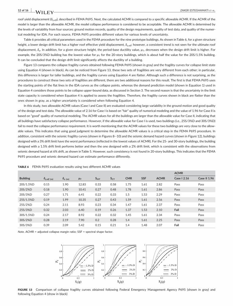
roof yield displacement (δy,eff), described in FEMA P695. Next, the calculated ACMR is compared to a specific allowable ACMR. If the ACMR of the

model is larger than the allowable ACMR, the model collapse performance is considered to be acceptable. The allowable ACMR is determined by

the levels of variability from four sources: ground motion records, quality of the design requirements, quality of test data, and quality of the numer-

ical modeling for IDA. For each source, FEMA P695 provides different values for various levels of uncertainty.

Table 6 provides all critical parameters used in the FEMA procedure for the nine prototype buildings. As shown inTable 6, for a given structure

height, a lower design drift limit has a higher roof effective yield displacement, δy,eff; however, a consistent trend is not seen for the ultimate roof

displacement, δu. In addition, for a given structure height, the period‐base ductility value, μT, decreases when the design drift limit is higher. For

example, the 20S/3%D building has the lowest value for μT for the 20‐story buildings, which is about half the value for the 20S/1.5% building.

It can be concluded that the design drift limit significantly affects the ductility of a building.

Figure 13 compares the collapse fragility curves obtained following FEMA P695 (shown in gray) and the fragility curves for collapse limit state

using Equation 4 (shown in black). As can be noticed from Figure 13, these two sets of fragilities are very different from each other; in particular,

this difference is larger for taller buildings, and the fragility curves using Equation 4 are flatter. Although such a difference is not surprising, as the

procedures to construct these two sets of fragilities are different, there are two additional reasons for this result. The first is that FEMA P695 uses

the starting points of the flat lines in the IDA curves as the collapse points, whereas the demand prediction model (shown in Equation 1) used in

Equation 4 considers those points to be collapse upper‐bound data, as discussed in Section 3. The second reason is that the uncertainty in the limit

state capacity is considered when Equation 4 is applied to assess the fragilities. Therefore, the fragility curves shown in black are flatter than the

ones shown in gray, as a higher uncertainty is considered when following Equation 4.

In this study, two allowable ACMR values (Case I and Case II) are evaluated considering large variability in the ground motion and good quality

of the design and test data. The allowable value of 2.16 for Case I is based on “fair” quality of numerical modeling and the value of 1.96 for Case II is

based on “good” quality of numerical modeling. The ACMR values for all the buildings are larger than the allowable value for Case II, indicating that

all buildings have satisfactory collapse performance. However, if the allowable value for Case I is used, two buildings (i.e., 25S/3%D and 30S/3%D)

fail to meet the collapse performance requirement. It is worth mentioning that the ACMR values for these two buildings are very close to the allow-

able values. This indicates that using good judgment to determine the allowable ACMR values is a critical step in the FEMA P695 procedure. In

addition, consistent with the seismic fragility curves (shown in Figures 8--10) and the seismic demand hazard curves (shown in Figure 12), buildings

designed with a 3% drift limit have the worst performance (reflected in the lowest values of ACMR). For the 25‐ and 30‐story buildings, the building

designed with a 1.5% drift limit performs better and then the one designed with a 2% drift limit, which is consistent with the observations from

seismic demand hazard at 6% drift, as shown inTable 5. However, such consistency is not found in 20‐story buildings. This indicates that the FEMA

P695 procedure and seismic demand hazard can estimate performance differently.

TABLE 6 FEMA P695 evaluation results using two different ACMR values

Building δy,eff (m) δu (m) μT SMT SCT CMR SSF ACMR

ACMR

Case I 2.16 Case II 1.96

20S/1.5%D 0.15 1.90 12.83 0.33 0.58 1.75 1.61 2.82 Pass Pass

20S/2%D 0.18 1.90 10.41 0.27 0.48 1.78 1.61 2.86 Pass Pass

20S/3%D 0.27 1.71 6.41 0.22 0.33 1.5 1.53 2.29 Pass Pass

25S/1.5%D 0.19 1.99 10.35 0.27 0.43 1.59 1.61 2.56 Pass Pass

25S/2%D 0.24 2.11 8.93 0.23 0.34 1.47 1.61 2.37 Pass Pass

25S/3%D 0.32 2.03 6.40 0.19 0.26 1.37 1.53 2.10 Fail Pass

30S/1.5%D 0.24 2.17 8.92 0.22 0.32 1.45 1.61 2.34 Pass Pass

30S/2%D 0.28 2.19 7.90 0.2 0.28 1.4 1.61 2.25 Pass Pass

30S/3%D 0.39 2.09 5.42 0.15 0.21 1.4 1.48 2.07 Fail Pass

Note. ACMR = adjusted collapse margin ratio; SSF = spectral shape factor.

FIGURE 13 Comparison of collapse fragility curves obtained following Federal Emergency Management Agency P695 (shown in gray) andfollowing Equation 4 (show in black)

ZAKER ESTEGHAMATI ET AL. 13 of 16

Compared with seismic demand hazard (which gives the annual probability of exceeding a given demand), the ACMR value can be considered

as a simplified proxy to represent seismic performance. There are two major drawbacks to using FEMA P695 procedure. One is that the allowable

ACMR value, a critical value in the procedure, is determined subjectively based on individual judgment. The other is that the determination of SSF

using pushover analysis is based on the first mode. This could be an issue, particularly for high‐rise buildings, as more than one mode will typically

dominate the dynamic behavior of a high‐rise building.

6 | CONCLUSIONS

The major contribution of this study is to provide a better understanding of the relationship between the design drift limit and the structural

performance of tall buildings. In this study, nine dual systems with the shear wall–frame system are used to evaluate the impact of design drift limit

on the seismic performance of high‐rise buildings. Three configurations (20‐, 25‐, and 30‐story buildings) are considered; for each configuration,

three structures are designed for different drift limits: ASCE 7 code specified limit (2%), a value lower than the code limit (1.5%), and a value higher

than the code limit (3%). The seismic performance is evaluated using seismic fragilities, seismic demand hazard, and collapse evaluation using the

FEMA P695 procedure. Finite element models of the nine prototype buildings are developed in OpenSees, and IDA is performed to capture build-

ing behavior from the elastic state to the point of collapse. The numerical results are used to develop probabilistic seismic demand models, where

the model parameters are evaluated using MLE to incorporate equality data and censored data (i.e., lower‐ and upper‐bound data). Seismic fragility

curves are developed using reliability analysis and are compared for four performance levels (immediate occupancy, life safety, collapse prevention,

and collapse). Seismic demand hazard curves are assessed by incorporating the seismic intensity hazard at the building location. Collapse perfor-

mance of prototype buildings is also compared following the FEMA P695 procedure.

The following summarizes the major findings regarding the relationship between the design drift limit and structural performance of tall

buildings in this study:

• Overall, the design drift limit affects the seismic performance of a high‐rise building, and this effect varies for various performance levels.

• Based on the fragility curve comparison, for a given seismic intensity, a design with a lower drift limit improves a building's performance for the

four performance levels considered.

• Based on the seismic demand hazard results, it is found that for the 30‐story configuration, using a more relaxed drift limit than the code limit is

cost‐effective, as it results in a similar structural performance as using the code design limit with smaller cross sections for columns and beams

in the frame. This implies that for high‐rise buildings, using a larger drift design limit can be beneficial.

• Based on seismic demand hazard results, it is found that for the 20‐story configuration, using a value smaller than the code design limit not only

results in a lower demand hazard but also yields larger cross sections in the frame members. This implies that for high‐rise buildings, using a

more restrained drift design limit does not necessarily improve the structure's seismic performance.

Other findings in the study are listed in the following:

• Based on the IDA results, 6% is found to be an appropriate mean value for the collapse limit.

• Seismic demand hazard results show that the building with better performance in one limit state does not necessarily have better performance

in another limit state. Therefore, considering a single performance level would not achieve an optimal design, which is consistent with the

findings of many other studies (e.g., LATBSDC,[47] Tuna and Wallace,[48] Dyanati et al.[50]).

• The result indicates that using fragility alone is not sufficient for comparison of the seismic performance of structures when a period‐dependent

IM is used to compare structures with different fundamental periods.

• Under seismic loading, the collapse mean annual frequencies of all buildings are smaller than the collapse objective of the ASCE 7 code,

indicating that the high‐rise structures are not collapse‐critical, a finding that is consistent with those from other studies (e.g., Haselton

et al.,[16] Jalali et al.,[17] Asgarian et al.[18]).

• In terms of collapse performance, the FEMA P695 procedure results are generally consistent with seismic fragility and demand hazard for most

of the buildings considered. However, the critical quantity used in FEMA P695 procedure, which is the allowable ACMR, largely depends on

judgment. Different ACMR values could determine whether a prototype yields an acceptable or unacceptable collapse performance.

• The FEMA P695 evaluation is a subjective procedure, and the ACMR value obtained for each building is a simplified proxy to reflect the seismic

performance of the structure; thus, it is less reliable as compared to direct probabilistic approaches (i.e., seismic fragility and demand hazard).

It should be noted that the conclusions obtained in this study are restricted to the drift limit ranges and the nine prototype buildings that are

examined here. In addition, other types of loadings, such as wind loads, are not in the scope of this paper. Therefore, the effectiveness of the ASCE

7 drift provision on high‐rise building performance requires future research to consider different loads, other types of high‐rise buildings,

14 of 16 ZAKER ESTEGHAMATI ET AL.

nonstructural component performance, and human comfort. Such important issues should be considered in future research regarding design pro-

visions for tall buildings.

ORCID

Mohsen Zaker Esteghamati http://orcid.org/0000-0002-2144-2938

Mehdi Banazadeh http://orcid.org/0000-0002-2309-392X

REFERENCES

[1] J. Gabel, M. Carver, M. Gerometta, Ctbuh 2016, (1).

[2] A. Bayraktar, A. Altunisik, T. Türker, H. Karadeniz, S. Erdogdu, Z. Angin, T. S. Özsahin, J. Perform. Constr. Facil. 2013, 29(6), 4014177. https://doi.org/10.1061/(ASCE)CF.1943‐5509.0000524

[3] B. Alemdar, A. A. Can, M. Murat, J. Perform. Constr. Facil. 2016, 30(2). https://doi.org/10.1061/(ASCE)CF.1943‐5509.0000383

[4] J. P. Moehle, Struct. Des. Tall Special Build. 2007, 16(5), 559. https://doi.org/10.1002/tal.435

[5] PEER, Guidelines for Performance‐Based Siesmic Design of Tall buildings, Pacific earthquake engineering research center, Berkeley, California 2010.

[6] M. Lew, F. Naeim, M. Hudson, B. Korin, Challenges in specifying ground motions for design of tall buildings in high seismic regions of the United States.14th World Conf. Earthq. Eng. 2008.

[7] ASCE Stand. American society of civil engineers/structural engineering institute, Reston, Virginia. 2010. https://doi.org/10.1061/9780784412916

[8] J. Moehle, G. G. Deierlein, 13th World Conf. Earthq. Eng. 2004. https://doi.org/10.1061/9780784412121.173

[9] R. D. Bertero, V. V. Bertero, Earthq. Eng. Struct. Dyn. 2002, 31(3), 627. https://doi.org/10.1002/eqe.146

[10] G. G. Deierlein, H. Krawinkler, C. A. Cornell, 2003 Pacific Conf. Earthq. Eng. 2003. https://doi.org/10.1061/9780784412121.173

[11] K. A. Porter, 9th Int. Conf. Appl. Stat. Probab Civ. Eng. 2003, 273(1995), 973.

[12] C. A. Goulet, C. B. Haselton, J. Mitrani‐Reiser, J. L. Beck, G. G. Deierlein, K. A. Porter, J. P. Stewart, Earthq. Eng. Struct. Dyn. 2007, 36(13), 1973. https://doi.org/10.1002/eqe.694

[13] H. A. El Howary, S. S. F. Mehanny, Earthq. Eng. Struct. Dyn. 2011, 40(2), 215. https://doi.org/10.1002/eqe.1016

[14] M. Shokrabadi, M. Banazadeh, M. Shokrabadi, A. Mellati, Eng. Struct. 2015, 98, 14. https://doi.org/10.1016/j.engstruct.2015.03.057

[15] S. H. Jeong, A. M. Mwafy, A. S. Elnashai, Eng. Struct. 2012, 34, 527. https://doi.org/10.1016/j.engstruct.2011.10.019

[16] C. B. Haselton, A. B. Liel, G. G. Deierlein, B. S. Dean, J. H. Chou, J. Struct. Eng. 2011, 137(4), 481. https://doi.org/10.1061/(ASCE)ST.1943‐541X.0000318

[17] S. A. Jalali, M. Banazadeh, E. Tafakori, A. Abolmaali, J. Constr. Steel Res. 2011, 67(8), 1261. https://doi.org/10.1016/j.jcsr.2011.03.008

[18] B. Asgarian, R. M. Nojoumi, P. Alanjari, Struct. Des. Tall Special Build. 2014, 23(2), 81. https://doi.org/10.1002/tal.1023

[19] A. Mathiasson, R. Medina, Buildings 2014, 4(4), 806. https://doi.org/10.3390/buildings4040806

[20] H. L. Sadraddin, X. Shao, Y. Hu, Struct. Design Tall Spec. Build. 2016, 25(18), 1089. https://doi.org/10.1002/tal.1299

[21] J. Pejovic, S. Jankovic, Bull. Earth. Eng. 2016, 14(1), 185. https://doi.org/10.1007/s10518‐015‐9812‐4

[22] H. S. Park, K. Hong, J. H. Seo, Struct. Des. Tall Build. 2002, 11(1), 35. https://doi.org/10.1002/tal.187

[23] F. Naeim The Seismic Design Handbook. Boston: Springer US; 2001. https://doi.org/10.1007/978‐1‐4615‐1693‐4

[24] B. S. Taranath, Reinforced Concrete Design of Tall Buildings, CRC press, First edit 2009.

[25] ACI, Building Code Requirements for Structural Concrete ( ACI 318–08 ). Farmington hills, Michigan, 2008. https://doi.org/10.1016/0262‐5075(85)90032‐6, 60

[26] S. Mazzoni, F. McKenna, M. H. Scott, G. L. Fenves, OpenSees command language manual, Pacific Earthq. Eng. Res. Cent. 2007, 451

[27] ATC, PEER. ATC 72‐1: Modeling and acceptance criteria for seismic design and analysis of tall buildings. Atc 72–1 2010.

[28] L. F. Ibarra, H. Krawinkler, A beam‐column joint model for simulating the earthquake response of reinforced concrete frames a beam‐column joint modelfor simulating the earthquake response of reinforced concrete frames, PEER Report 2003/10. 2004.

[29] F. Zareian, R. A. Medina, Comput. Struct. 2010, 88(1–2), 45. https://doi.org/10.1016/j.compstruc.2009.08.001

[30] L. F. Ibarra, H. Krawinkler, Global Collapse of Frame Structures under Seismic Excitations. Berkeley, California: 2005. https://doi.org/10.1002/eqe

[31] C. B. Haselton, A. B. Liel, S. T. Lange, Beam‐column element model calibrated for predicting flexural response leading to global collapse of RC framebuildings. Peer 2007 2008; 3(May).

[32] T. B. Panagiotakos, ACI Struct. J. 2001, 98(2), 135. https://doi.org/10.14359/10181

[33] K. Beyer, A. Dazio, M. J. N. Priestley, Proc. 2008.

[34] L. N. Lowes, P. Oyen, D. E. Lehman, Am. Concr. Inst., ACI SP 2009.

[35] R. E. Sedgh, R. P. Dhakal, A. J. Carr, N. Z. Soc. Earthq. Eng. 2015.

[36] P. Martinelli, F. C. Filippou, Earthq. Eng. Struct. Dyn. 2009, 38(5), 587. https://doi.org/10.1002/eqe.897

[37] J. B. Mander, M. J. N. Priestley, R. Park, J. Struct. Eng. 1988, 114(8), 1804. https://doi.org/10.1061/(ASCE)0733‐9445(1988)114:8(1804)

[38] D. Vamvatsikos, C. C. Allin, Earthq. Eng. Struct. Dyn. 2002, 31(3), 491. https://doi.org/10.1002/eqe.141

[39] FEMA. Quantification of building seismic performance factors Federal emergency management agency, (FEMA P695) Washington,D.C. 2009.

[40] D. Vamvatsikos, C. A. Cornell, Earthq. Spectra 2004, 20(2), 523. https://doi.org/10.1193/1.1737737

[41] K. C. Lin, C. C. J. Lin, J. Y. Chen, H. Y. Chang, Struc. Saf. 2010, 32(3), 174. https://doi.org/10.1016/j.strusafe.2009.11.001

ZAKER ESTEGHAMATI ET AL. 15 of 16

[42] P. Gardoni, A. Der Kiureghian, K. M. Mosalam, J. Eng. Mech. 2002, 128(10), 1024. https://doi.org/10.1061/(ASCE)0733‐9399(2002)128:10(1024)

[43] M. Dyanati, Q. Huang, D. Roke, Eng. Struct. 2015, 84, 368. https://doi.org/10.1016/j.engstruct.2014.11.036

[44] American Society of Civil Engineers (ASCE). FEMA 356 Prestandard and commentary for the seismic rehabilitation of building. Rehabilitation2000(November).

[45] ASCE. Seismic rehabilitation of existing buildings(ASCE/SEI 41‐06). American society of civil engineers, Reston, Virginia: American Society of Civil Engi-neers (ASCE); 2007. https://doi.org/10.1061/9780784408841

[46] Federal Emergency Management Agency (FEMA). HAZUS‐MH MR4 Technical Manual. National Institute of building sciences and Federal EmergencyManagement Agency (NIBS and FEMA) 2003: 712.

[47] LATBSDC, An alternative procedure for seismic analysis and design of tall buildings located in the Los Angeles region, Los Angeles, California 2008.

[48] Z. Tuna, J. W. Wallace, Seismic performance, modeling, and failure assessment of reinforced concrete Shear Wall buildings. University of California,LosAngeles, 2012.

[49] USGS. Unified hazard tool. https://earthquake.usgs.gov/hazards/interactive/ [accessed January 1, 2017].

[50] M. Dyanati, Q. Huang, D. Roke, Bull. Earthq. Eng. 2017, 15, 4751. (Asec 210). https://doi.org/10.1007/s10518‐017‐0150‐6

Mohsen Zaker Esteghamati received his B.Sc. In civil engineering from Iran University of Science and Technology. He has a M.Sc. instructural

engineering from Amirkabir University of Technology. Currently, he is a graduate assistant at University of Akron, where he is working on

ground motion selection impacts on seismic demand models.

Dr. Mehdi Banazadeh is an associate professor at civil and environmental engineering department of Amirkabir University. He received his Ph.

D. From Ryukyus University. His research interests include performance‐based earthquake engineering and nonlinear finite element modeling

of structures.

Dr. Qindan Huang is an assistant professor at the University of Akron. She received her Ph.D. from Texas A&M University. Her research

interests include reliability analysis and probabilistic modeling of structural performance.

How to cite this article: Zaker Esteghamati M, Banazadeh M, Huang Q. The effect of design drift limit on the seismic performance of RC

dual high‐rise buildings. Struct Design Tall Spec Build. 2018;27:e1464. https://doi.org/10.1002/tal.1464

APPENDIX

Table A1 | Frame section of the prototype buildings

Buildingconfiguration

No. ofstory

Design limit: 1.50%

ColumnBeam

Cross section (mm × mm) Rebar Cross section (mm × mm)

20‐story 1–5 900 × 900 (+26.5%)a 28ϕ28 (+16.7%) 900 × 800 (+28.5%)6–10 800 × 800 (+13.8%) 24ϕ28 (+20.0%) 800 × 750 (+14.3%)11–15 750 × 750 (+14.8%) 20ϕ28 (0.0%) 750 × 750 (+33.9%)16–20 650 × 650 (0.0%) 16ϕ28 (0.0%) 650 × 650 (+8.3%)

25‐story 1–5 950 × 950 (+11.4%) 32ϕ28 (+14.3%) 950 × 800 (+12.6%)6–10 900 × 900 (+12.1%) 28ϕ28 (+16.7%) 900 × 800 (+21.0%)11–15 800 × 800 (+13.8%) 24ϕ28 (0.0%) 800 × 800 (+21.9%)16–20 700 × 700 (+16.0%) 20ϕ28 (0.0%) 700 × 800 (+23.1%)21–25 600 × 600 (0.0%) 16ϕ28 (0.0%) 600 × 700 (+7.7%)

30‐story 1–5 950 × 950 (0.0%) 32ϕ28 (0.0%) 900 × 950 (+12.5%)6–10 900 × 900 (0.0%) 28ϕ28 (0.0%) 900 × 900 (+12.5%)11–15 850 × 850 (+12.9%) 24ϕ28 (0.0%) 850 × 900 (+19.5%)16–20 750 × 750 (+14.8%) 20ϕ28 (0.0%) 750 × 900 (+20.5%)21–25 650 × 650 (+17.4%) 16ϕ28 (0.0%) 650 × 900 (+39.3%)26–30 550 × 550 (+21.0%) 12ϕ28 (0.0%) 550 × 800 (+25.7%)

aPercentage of change compared to the corresponding value in the building with design limit of 2%.

Buildingconfiguration

Design limit: 2% Design limit: 3%

ColumnBeam

ColumnBeam

Cross section (mm × mm) Rebar Cross section (mm × mm) Cross section (mm × mm) Rebar Cross section (mm × mm)

20‐story 800 × 800 24ϕ28 800 × 700 700 × 700 (−30.6%) 20ϕ28 (−16.7%) 700 × 550 (−31.3%)750 × 750 20ϕ28 750 × 700 650 × 650 (−24.9%) 20ϕ28 (0.0%) 650 × 550 (−31.9%)700 × 700 20ϕ28 700 × 600 600 × 600 (−26.5%) 16ϕ28 (−20.0%) 600 × 500 (−22.6%)650 × 650 16ϕ28 650 × 600 500 × 500 (−40.8%) 12ϕ28 (−25.0%) 500 × 500 (−35.9%)

25‐story 900 × 900 28ϕ28 900 × 750 800 × 800 (−20.1%) 20ϕ28 (−28.6%) 800 × 650 (−23.0%)850 × 850 24ϕ28 850 × 700 750 × 750 (−22.2%) 20ϕ28 (−16.7%) 700 × 650 (−23.5%)750 × 750 24ϕ28 750 × 700 650 × 650 (−24.9%) 16ϕ28 (−33.3%) 650 × 650 (−19.5%)650 × 650 20ϕ28 650 × 700 600 × 600 (−14.8%) 12ϕ28 (−40.0%) 600 × 600 (−20.9%)600 × 600 16ϕ28 600 × 650 500 × 500 (−30.6%) 12ϕ28 (−25.0%) 500 × 500 (−35.9%)

30‐story 950 × 950 32ϕ28 950 × 800 850 × 850 (−19.9%) 28ϕ28 (−12.5%) 750 × 600 (−40.8%)900 × 900 28ϕ28 900 × 800 750 × 750 (−30.6%) 24ϕ28 (−14.3%) 700 × 600 (−41.7%)800 × 800 24ϕ28 800 × 800 700 × 700 (−23.4%) 20ϕ28 (−16.7%) 650 × 600 (−39.1%)700 × 700 20ϕ28 700 × 800 650 × 650 (−13.8%) 20ϕ28 (0.0%) 600 × 600 (−35.7%)600 × 600 16ϕ28 600 × 700 600 × 600 (0.0%) 16ϕ28 (0.0%) 500 × 500 (−40.5%)500 × 500 12ϕ28 500 × 700 500 × 500 (0.0%) 12ϕ28 (0.0%) 500 × 500 (−28.6%)

16 of 16 ZAKER ESTEGHAMATI ET AL.

Table A2 | Shear wall section of prototype buildings

Buildingconfiguration

No. ofstory

Design limit: 1.50% Design limit: 2% Design limit: 3%

Thickness (mm) Reinforcement Thickness (mm) Reinforcement Thickness (mm) Reinforcement

20‐story 1–5 450 (0.0%)a ϕ25@150 (0.0%) 450 ϕ25@150 350 (−22.2%) ϕ28@150 (+12.0%)6–10 450 (0.0%) ϕ20@250 (0.0%) 450 ϕ20@250 350 (−22.2%) ϕ20@250 (0.0%)11–20 350 (0.0%) Φ16@250 (−20.0%) 350 ϕ20@250 250 (−28.6%) ϕ20@250 (0.0%)

25‐story 1–5 500 (+11.1%) ϕ25@150 (0.0%) 450 ϕ25@150 350 (−22.2%) ϕ28@150 (+12.0%)6–10 500 (+11.1%) ϕ20@250 (0.0%) 450 ϕ20@250 350 (−22.2%) ϕ20@250 (0.0%)11–13 500 (+11.1%) Φ16@250 (−20.0%) 450 ϕ20@250 350 (−22.2%) ϕ20@250 (0.0%)14–25 400 (+14.3%) Φ16@250 (−20.0%) 350 ϕ20@250 250 (−28.6%) ϕ20@250 (0.0%)

30‐story 1–5 600 (+33.3%) ϕ25@150 (0.0%) 450 ϕ25@150 450 (0.0%) ϕ25@150 (0.0%)6–13 600 (+33.3%) ϕ20@250 (0.0%) 450 ϕ20@250 450 (0.0%) ϕ20@250 (0.0%)14–30 400 (+14.3%) ϕ20@250 (0.0%) 350 ϕ20@250 350 (0.0%) ϕ20@250 (0.0%)

aPercentage of change compared to the corresponding value in the building with design limit of 2%.

View publication statsView publication stats