the effect of thickness in the through-diffusion experiment · after the ending of the...
TRANSCRIPT

VTT TIEDOTTEITA – MEDDELANDEN – RESEARCH NOTES 1788
TECHNICAL RESEARCH CENTRE OF FINLANDESPOO 1996
The effect of thicknessin the through-diffusion experiment
Final report
Matti Valkiainen, Hannu Aalto, Jarmo Lehikoinen &
Kari Uusheimo
VTT Chemical Technology

ISBN 951-38-4983-XISSN 1235–0605Copyright © Valtion teknillinen tutkimuskeskus (VTT) 1996
JULKAISIJA – UTGIVARE – PUBLISHER
Valtion teknillinen tutkimuskeskus (VTT), Vuorimiehentie 5, PL 2000, 02044 VTTpuh. vaihde (09) 4561, faksi (09) 456 4374
Statens tekniska forskningscentral (VTT), Bergsmansvägen 5, PB 2000, 02044 VTTtel. växel (09) 4561, fax (09) 456 4374
Technical Research Centre of Finland (VTT), Vuorimiehentie 5, P.O.Box 2000, FIN–02044 VTT, Finlandphone internat. + 358 9 4561, fax + 358 9 456 4374
VTT Kemiantekniikka, Ympäristötekniikka, Otakaari 3 A, PL 1404, 02044 VTTpuh. vaihde (09) 4561, faksi (09) 456 6390
VTT Kemiteknik, Miljöteknik, Otsvängen 3 A, PB 1404, 02044 VTTtel. växel (09) 4561, fax (09) 456 6390
VTT Chemical Technology, Environmental Technology, Otakaari 3 A, P.O.Box 1404,FIN–02044 VTT, Finlandphone internat. + 358 9 4561, fax + 358 9 456 6390
Technical editing Leena Ukskoski
VTT OFFSETPALVELU, ESPOO 1996

3
Valkiainen, Matti, Aalto, Hannu, Lehikoinen, Jarmo & Uusheimo, Kari. The effect of thickness in thethrough-diffusion experiment. Final Report [Paksuuden vaikutus läpidiffuusiokokeessa. Loppuraportti].Espoo 1996, Technical Research Centre of Finland, VTT Tiedotteita - Meddelanden - Research Notes1788. 30 p. + app. 3 p.
UDC 552:532.72:552.32
Keywords rocks, granite, rock mechanics, rock properties, diffusion, porosity, water, thickness,measurement, experimentation
ABSTRACT
This report contains an experimental study of diffusion in the water-filled pores of rocksamples. The samples studied are rapakivi granite from Loviisa, southern Finland. Thedrill-core sample was sectioned perpendicularly with a diamond saw and threecylindrical samples were obtained. The nominal thicknesses (heights of the cylinders)are 2, 4 and 6 cm. For the diffusion measurement the sample holders were pressedbetween two chambers. One of the chambers was filled with 0.0044 molar sodiumchloride solution spiked with tracers. Another chamber was filled with inactive solution.Tritium (HTO) considered to be a water equivalent tracer and anionic 36Cl were used astracers.
The through diffusion was monitored about 1000 days after which time the diffusioncells were emptied and the sample holders dismantled. The samples were sectioned into1 cm slices and the tracers were leached from the slices. The porosities of the sliceswere determined by the weighing method.
The rock-capacity factors could be determined from the leaching results obtained. It wasseen that the porosity values were in accordance with the rock capacity factors obtainedwith HTO. An anion exclusion can be seen comparing the results obtained with HTOand 36Cl-. The concentration profile through even the thickest sample had reached aconstant slope and the rate of diffusion was practically at a steady state. An anionexclusion effect was also seen in the effective diffusion coefficients.
The effect of thickness on diffusion shows that the connectivity of the pores decreasesin the thickness range 2 - 4 cm studied. The decrease as reflected in the diffusioncoefficient was not dramatic and it can be said that especially for studying chemicalinteractions during diffusion, the thickness of 2 cm is adequate.

4
Valkiainen, Matti, Aalto, Hannu, Lehikoinen, Jarmo & Uusheimo, Kari. The effect of thickness in thethrough-diffusion experiment. Final Report [Paksuuden vaikutus läpidiffuusiokokeessa. Loppuraportti].Espoo 1996, Technical Research Centre of Finland, VTT Tiedotteita - Meddelanden - Research Notes1788. 30 p. + app. 3 p.
UDC 552:532.72:552.32
Keywords rocks, granite, rock mechanics, rock properties, diffusion, porosity, water, thickness,measurement, experimentation
TIIVISTELMÄ
Tämä raportti perustuu Loviisan rapakivigraniittinäytteillä tehtyyn matriisidiffuu-siotutkimukseen, jossa tutkittiin näytteen paksuuden vaikutusta diffuusioon. Näytteetsahattiin timanttilaikalla kairansydämestä akselia vastaan kohtisuoraan ja niidenpaksuuksiksi valittiin 2, 4 ja 6 cm. Diffuusiokokeet tehtiin läpidiffuusiogeometriassa,jossa näyte on sijoitettuna kahden nestetäytteisen kammion väliin. Kammiot täytettiin0,0044 molaarisella natriumkloridiliuoksella. Toiseen kammioista panostettiin merkki-ainetta. Tritium (HTO), joka on vesiuskollinen merkkiaine, oli toisena komponenttina jaanioninen 36Cl toisena komponenttina.
Läpidiffuusiota seurattiin noin 1 000 päivän ajan, jonka jälkeen diffuusiokammiottyhjennettiin ja näytteenpitimet purettiin. Näytteet viipaloitiin 1 cm:n paksuisiksi javiipaleista eluoitiin merkkiaineet. Näytteiden huokoisuus määritettiin punnitusmenetel-mällä.
Näytteiden kapasiteettitekijät voitiin määrittää eluutiotuloksista. Tritium-kapasiteettitekijät ja punnitushuokoisuustulokset olivat sangen yhtäpitäviä. Kunverrataan HTO ja 36Cl- tuloksia, nähdään selvä anioniekskluusio, joka näkyy myösefektiivisissä diffuusiokertoimissa; osoittautui myös, että paksuinkin näyte olisaavuttanut vakiodiffuusionopeuden.
Diffuusiotuloksista voidaan päätellä, että tutkitulla rapakivigraniitilla huokosreittienliityntä toisiinsa vähenee alueella 2 - 4 cm. Väheneminen ole suuruudeltaandramaattista, ja voidaan päätellä, että varsinkin kemiallisten vuorovaikutustentutkimisessa on ohuin, 2 cm:n näyte riittävän paksu.

5
FOREWORD
This report forms the second part of a laboratory study of matrix diffusion in granitesamples of different thicknesses. The previous part of the report is published in VTTResearch Notes number 1556. The theoretical part (Chapter 2) is taken as such fromthe previous report, but the results are described concentrating on the new resultsafter approximately one additional year of experimental time and the measures takenafter the ending of the through-diffusion experiment.
The help of Kirsti Helosuo in the sampling of the diffusion test and that of SeppoJuurikkala in the sectioning of the samples is appreciated. The liquid scintillationanalysis of the samples was continued by Hannu Aalto after the death of KariUusheimo in 1994.

6
CONTENTS
ABSTRACT................................................................................................................. 3
TIIVISTELMÄ............................................................................................................. 4
FOREWORD ............................................................................................................. 5
CONTENTS ................................................................................................................ 6
1 INTRODUCTION.................................................................................................. 7
2 DIFFUSION IN POROUS MATERIAL............................................................... 8
3 EXPERIMENTAL................................................................................................ 123.1 Rock samples and diffusion measurements................................. 12
3.1.1 Rock samples...................................................... 123.1.2 Diffusion experiment.......................................... 12
3.2 Sectioning and leaching of the samples....................................... 143.3 Porosity measurement.................................................................. 16
4 RESULTS 174.1 Diffusion of the tracers ................................................................ 17
4.1.1 Approaching the steady state.............................. 194.2 Leaching of the sub-samples ....................................................... 204.3 Water-saturation porosities.......................................................... 234.4 Fitting of the diffusion model ...................................................... 23
5 DISCUSSION OF THE RESULTS...................................................................... 24
6 SUMMARY AND CONCLUSIONS................................................................... 27
REFERENCES.......................................................................................................... 29
APPENDIX 1
THE DERIVATIVES OF THE EXPERIMENTAL RESULTS

7
1 INTRODUCTION
Transport by diffusion from water-conducting fractures in a narrow pore networkextending into the rock matrix is considered an important retardation mechanism innuclear waste disposal. Radionuclides spread in the available pore space adjoiningthe fractures by diffusion.
In the laboratory the diffusion coefficients in the water phase are often determinedfrom samples with rather short linear dimensions due to time limitations. In thisstudy, the diffusion test is performed using three samples of rapakivi granite ofdifferent thicknesses. The samples were originally situated close to each other. Theaim was to ensure the maximum possible homogeneity between the samples. Thetracers used were tritium and 36Cl.
It has been reported in the literature /1, 2, 3/ that the geometrical formation factormeasured for the rock samples decreases when the thickness of the sample increases.Because the geometrical formation factor F = ε+σ/τ2, where ε+ is the conductingporosity and τ the length of the diffusion path divided by the thickness of the sample,tortuosity, it might be possible to see the effect of the sample thickness on theconductive porosity.
It was shown by Hemingway, Bradbury and Lever /4/ that the simple Fickian modeldoes not provide a complete description of the concentration-time curves obtainedfor laboratory diffusion experiments. A new model was developed taking intoaccount that some of the diffusion paths are dead-ends. The model characterizesdead-end pores with two parameters: the fraction of dead-end porosity from the totalporosity and the average length of the dead-end pores.
The dead-end porosity model gives the same asymptotic behaviour and thus thesame time-lag in through-diffusion geometry. A significant improvement for theinterpretation of small-scale laboratory through-diffusion experiments was found.The fit of calculated diffusion behaviour to experimental data was found to betterexplain the pre-steady-state period of the through-diffused concentration.
Although the dead-end pore model better explains the laboratory-scale experiments,the conventional Fickian model was found to be adequate under all conditions likelyto arise around the repository.
The tracers selected were tritium (HTO) and anionic 36Cl, easily analyzable by liquidscintillation counting. Both are considered as minimally sorbing. 36Cl is speciated aschloride, thus repulsive forces are expected between the ions and the pore walls. Inthe case of tritium, some interaction with the pore walls can be expected.

8
2 DIFFUSION IN POROUS MATERIAL
In the following model it is assumed that the concentration in the porewater is thesame as in the surrounding water. The pores form a branching tortuous labyrinth,some branches are forming dead ends. Thus the porosity may be divided in twocategories: through-transport and dead-end porosity. The rock-capacity factor is alsodivided in the same ratio in those two categories. The dead-end porosity concept hasbeen applied to rock diffusion by Hemingway et al. at Harwell /4/ and laterLehikoinen et al. /5/. The governing equation of their dead-end pore diffusionmodels is
and
whereC+=C+(x,t) = concentration in the conductive pores,C*=C*(x,t) = concentration in the dead-end pores,De = effective diffusion coefficient1,α+ = rock-capacity factor of the conductive pores,α* = rock-capacity factor of the dead-end pores,tt = relaxation time (characteristic time for diffusion into dead-end
pores).
The partial differential equations (1a) and (1b) are solved in one dimension using thefollowing trial function, which fulfils the initial condition C(x,0)=0 and boundaryconditions C(0,t)=C1 and C(l,t)=0.
1
The effective diffusion coefficient and the diffusion coefficient in an unconfined fluid are related through the so-calledformation factor F: De= F × Dw. The pore structure parameters and F can be interrelated. Skagius /4/ uses F = ε+σ/τ2, whereσ is the constrictivity. The formation factor will thus be smaller than unity. Inverse notation is also used (e. g. Katsube et al./5/).
+++
+ ∇=∂
∂α+∂
∂α CDt
Ct
Ce
* 2 (1a)
)CC(tt
C *
t
*
−=∂
∂ +1(1b)
9
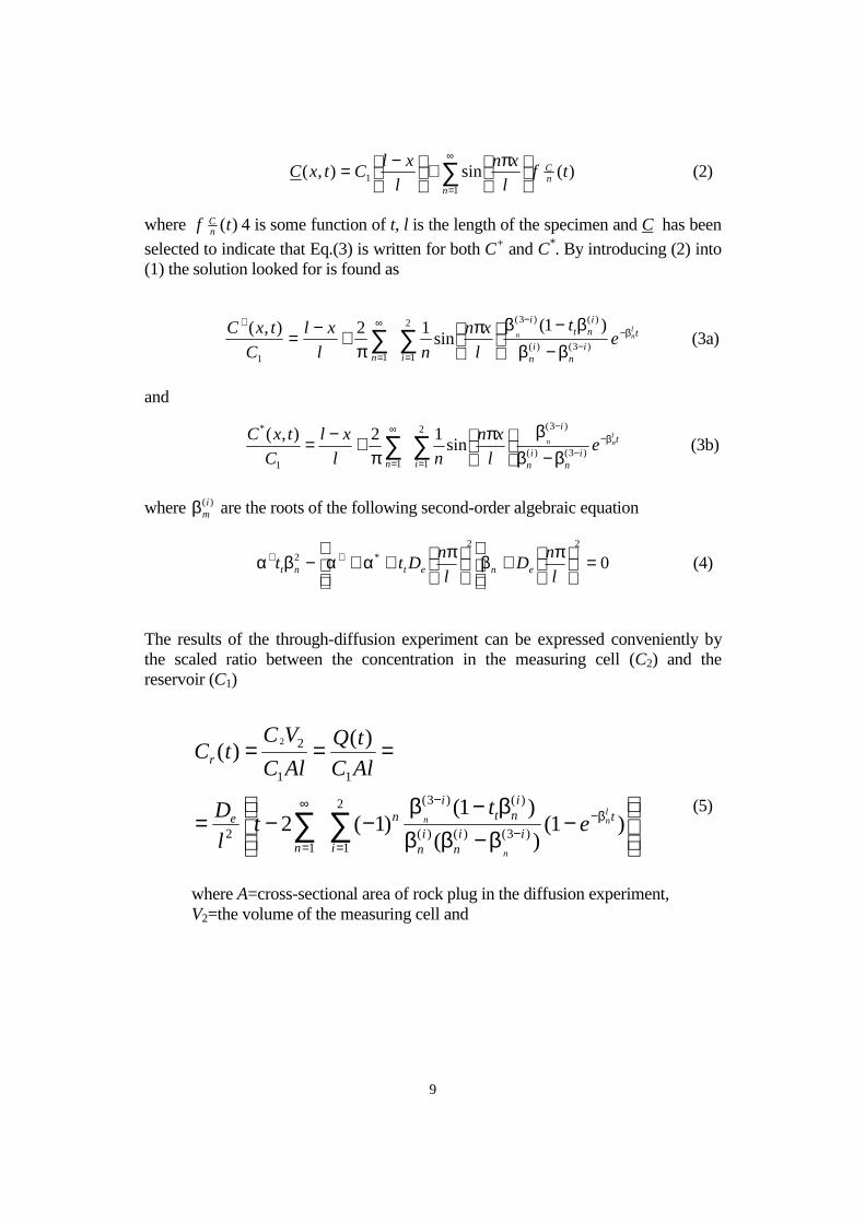
where )(tf nC 4 is some function of t, l is the length of the specimen and C has been
selected to indicate that Eq.(3) is written for both C+ and C*. By introducing (2) into(1) the solution looked for is found as
and
where )(imβ are the roots of the following second-order algebraic equation
The results of the through-diffusion experiment can be expressed conveniently bythe scaled ratio between the concentration in the measuring cell (C2) and thereservoir (C1)
)(sin),(1
1 tfl
xn
l
xlCtxC n
C
n
π+
−= ∑
∞
=
(2)
ti
ni
n
int
i
in
lnn e
t
l
xn
nl
xl
C
txC β−−
−
=
∞
=
+
β−ββ−β
π
π+−= ∑∑ )3()(
)()3(2
111
)1(sin
12),((3a)
ti
ni
n
i
in
lnn e
l
xn
nl
xl
C
txC β−−
−
=
∞
= β−ββ
π
π+−= ∑∑ )3()(
)3(2
111
*
sin12),(
(3b)
022
*2 =
π+β
π+α+α−βα ++
l
nD
l
nDtt enetnt (4)
−β−βββ−β
−−=
===
∑∑=
β−−
−∞
=
2
1)3()()(
)()3(
12
11
2
)1()(
)1()1(2
)()(
2
i
tii
ni
n
int
in
n
e
r
ln
n
n et
tl
D
AlC
tQ
AlC
VCtC
(5)
where A=cross-sectional area of rock plug in the diffusion experiment,V2=the volume of the measuring cell and

10
where A=cross-sectional area of rock plug in the diffusion experiment, V2=thevolume of the measuring cell and
corresponding to the diffused amount for the time t.
By scaling the time by the square of the thickness, the results of the samples ofdifferent thicknesses can be presented in the same t/l2, (C2V2)/(C1Al) -co-ordinates.As an example, we can take three rock samples, thicknesses 2, 4 and 6 cm. De =2.3 x 10⁻¹³ m2/s, α = 0.004, dead-end-pore length lde ≈ (3ttDe/α+)½ = 2 cm andε+/(α++ε*) = 0.5.
Figure 1. The initial period in diffusion experiment, calculated results for threeexamples, thicknesses 2, 4 and 6 cm. De = 2.3 x 10⁻¹³ m2/s, α =0.004, length of thedead-end pores lde = 2 cm and ε+/(α++ε*) = 0.5. The diffusion curves are scaled tothe same scale and all have the same asymptote. The curve applying to all examplesin the case without dead-end porosity is the lowest.
tdx
txCADtQ x
t
e ′∂
′∂−= =
+
∫ 10
),()( (6)

11
Figure 1 depicts the initial part of the calculated through diffusion. It can be seen thatthe effect of dead-end porosity is more pronounced in thinner samples. When thesamples are thicker, the diffusion behaviour approaches the simple case, not takinginto account dead-end porosity in calculations /6/
where α = α++α*. The asymptotic behaviour of Eq.(7), as t→∞, is given by the line
,exp)1(2
6)( 2
22
21
22
απ−
πα−α−= ∑
∞
= l
tnD
nl
tDtC e
n
n
er (7)
6)(
2
α−=l
tDtC e
r

12
3 EXPERIMENTAL
3.1 ROCK SAMPLES AND DIFFUSION MEASUREMENTS
3.1.1 Rock samples
During site selection studies for a repository for low and medium-level reactorwaste, drill-holes were made at Hästholmen, Loviisa. Drill-core samples wereobtained from Imatran Voima Oy originating from drill-hole Y1 between 195.15 mand 195.51 m. The rock is fine-grained rapakivi granite. The drill-core sample wassectioned perpendicularly with a fast, water-cooled diamond saw and threecylindrical samples were obtained. The nominal thicknesses (heights of thecylinders) were 2, 4 and 6 cm.
3.1.2 Diffusion experiment
The rock samples were fixed with silicone glue to cylindrical openings in PVCframes of 2 mm larger diameter than the drill-cores, Figure 2.
Figure 2. Rock samples and sample holders made of PVC plastic.
After gluing, the rock samples were kept in the vacuum for 2 - 4 days to expel the airfrom the pore space. While in the vacuum, sodium chloride solution

13
(0.0044 molar) was put into contact with the samples. They were allowed toequilibrate with the solution for 1 - 10 months. For the diffusion measurement, thesample holders were pressed between two chambers 64 ml each in volume (Figure3). One of the chambers was filled with 0.0044 molar sodium chloride solutionspiked with tracers. Another chamber was filled with inactive solution. Tritium(HTO) considered to be a water-equivalent tracer and anionic 36Cl were used astracers. The initial activity concentrations were with 2 cm and 4 cm samples about 2µCi/ml about 1 µCi/ml for tritium and 36Cl, respectively. More activity was usedwith the thickest sample, about 8 µCi/ml HTO and 4 µCi/ml chloride-36.
Figure 3. The experimental setup for the diffusion measurement, the rock sampleseparates the two liquid-filled chambers.
Table 1 shows a summary of the characteristics of the samples and equilibrationtimes.

14
Table 1. Summary of the characteristics of the samples and equilibration times.
Sample Length Weight Diameter Equilibration time
(mm) (g) (mm) (Months)
C1 19.3 104.66 51.6 1
C2 39.3 213.63 51.6 4
C3 58.8 320.65 51.6 10
The experiment was followed by taking samples from the originally inactivechamber. The water in the chamber had turned slightly radioactive. To begin thesamples were taken originally weekly, later monthly. The chamber was emptiedfully and filled again with new inactive solution. A sample of 10 ml was taken fromthe used solution for determination of the 3H and 36Cl content of the solution with aliquid scintillation counter.
3.2 SECTIONING AND LEACHING OF THE SAMPLES
The diffusion experiment was monitored over 1000 days, after which it wasconsidered to have given all the essential information obtainable from the performedtest phase. The measurement was interrupted by emptying and flushing thechambers. The rock specimens were removed from the PVC frames and slicedperpendicularly to the axis with a slow-speed diamond saw. Figure 4 presents thesample codes given to identify the sectioned samples. During sawing the sampleslost some water and tracers. To minimize this, aluminium foil was used to wrap thesamples to the extent possible.
The samples were leached individually at 100 ml of 0.044 Mol NaCl solution,initially free of radioactive tracers. The leachant was sampled regularly for activitydetermination and the sample was replaced with fresh solution. The leaching wasmonitored for 170 days.

15
Figure 4. Sectioning and coding of the rock samples after the through-diffusionexperiment.

16
3.3 POROSITY MEASUREMENT
The porosity of the sectioned sub-samples was measured after the leaching by amodified method of the Melnyk & Skeet-method /7/. The essential part of themethod is the determination of the surface-dry, otherwise water-saturated weight ofthe sample by monitoring of the initial part of the drying process.
The rock slices were assumed to be completely water saturated after the leaching.They were weighed in water (one at a time), the extra moisture on the surface wasslightly wiped off before placing in a balance, where the weight-loss duringevaporation was monitored. Figure 5 shows the weight as a function of time for oneof the sub-samples and determination of the surface-dry weight as the crossing pointof two asymptotes.
Figure 5. Determination of surface-dry weight as the crossing point of twoasymptotes of the drying curve /7/.

17
4 RESULTS
4.1 DIFFUSION OF THE TRACERS
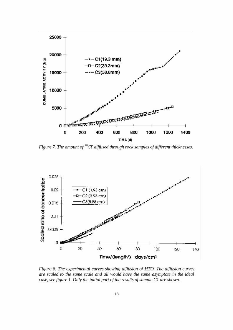
Figures 6 and 7 show the cumulative amount of tracer diffused through thespecimens as a function of time. The results are scaled to the same initial activity.There are disturbances in the final part of the experiment with the 2 cm sample, andtherefore the 5 last data points were rejected.
Figure 6. The amount of tritium diffused through rock samples of differentthicknesses.
To simplify the presentation of the fitting of the experimental results, the data weretransformed to the same co-ordinates used in Figure 1; the co-ordinates reveal therelative evolution of the three parallel experiments. See Figures 7 and 8, where onlythe initial part of the results of sample C1 are shown.
18
Figure 7. The amount of 36Cl- diffused through rock samples of different thicknesses.
Figure 8. The experimental curves showing diffusion of HTO. The diffusion curvesare scaled to the same scale and all would have the same asymptote in the idealcase, see figure 1. Only the initial part of the results of sample C1 are shown.

19
Figure 9. The experimental curves showing diffusion of 36Cl-. The diffusion curvesare scaled to the same scale and all would have the same asymptote in the idealcase, see Figure 1. Only the initial part of the results of sample C1 are shown.
4.1.1 Approaching the steady state
The rate of the through-diffusion should stabilize to a constant value furnishing theeffective diffusion coefficient. The through-diffused incremental amounts arepresented as a function of time in Appendix 1. It can be said that the quality of thedata does not permit exact estimation of the steady state of the through-diffusion, butthe following can be stated.
- In the 2 cm sample the diffusion seems to obtain a stationary ratearound 200 days, but after that the rate rises again. This behaviour isnot seen with 36Cl.
- The 4 cm sample has achieved the steady-state phase.
- The 6 cm sample is at the beginning of the steady-state phase.
Visually estimated stationary levels gave the values for De given in Table 2.

20
Table 2. Effective diffusion coefficients estimated from the incremental amounts ofthe through-diffusion.
Effective diffusion coefficients (m2/s)
Tracer C1 (2 cm) C2 (4 cm) C3 (6 cm)3H 2.4 x 10⁻¹³ 2.2 x 10⁻¹³ 1.7 x 10⁻¹³
36Cl 5.4 x 10⁻¹⁴ 3.5 x 10⁻¹⁴ 2.2 x 10⁻¹⁴
4.2 LEACHING OF THE SUB-SAMPLES
The tracer distribution inside the sample at the end of the diffusion experiment isapproximately obtained from the leaching results of the sub-samples. Figure 10shows an example of diffusion of 3H and 36Cl from a sub-sample.
Figure 10. Leaching of tritium and 36Cl from the sub-sample C23.
21
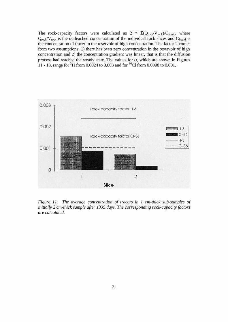
The rock-capacity factors were calculated as 2 * Σ(Qrock/Vrock)/Cliquid, whereQrock/Vrock is the outleached concentration of the individual rock slices and Cliquid isthe concentration of tracer in the reservoir of high concentration. The factor 2 comesfrom two assumptions: 1) there has been zero concentration in the reservoir of highconcentration and 2) the concentration gradient was linear, that is that the diffusionprocess had reached the steady state. The values for α, which are shown in Figures11 - 13, range for 3H from 0.0024 to 0.003 and for 36Cl from 0.0008 to 0.001.
Figure 11. The average concentration of tracers in 1 cm-thick sub-samples ofinitially 2 cm-thick sample after 1335 days. The corresponding rock-capacity factorsare calculated.

22
Figure 12. The average concentration of tracers in 1-cm thick sub-samples ofinitially 4-cm thick sample after 1248 days. The corresponding rock-capacity factorsare calculated.
Figure 13. The average concentration of tracers in 1 cm-thick sub-samples ofinitially 6-cm thick sample after 1080 days. The corresponding rock-capacity factorsare calculated.

23
4.3 WATER-SATURATION POROSITIES
The porosity values in Table 3 are obtained from the weight difference of thesaturated, surface-dry sample and the same sample, dried at elevated temperature.The drying was carried out for four weeks at 40 oC and subsequently for two weeksat 60 oC.
Table 3. Porosities of the sub-samples evaluated from the weight loss during drying.
Sample codeWeight inwater(g)
Weight (g)Surface dry
Weight (g)Dried105 d
DensitySaturated(g/cm3)
Porosity
C11 30.47 48.96087 48.9042 2.65 0.31%
C12 33.2 53.42751 53.3604 2.64 0.33%
C21 32.44 52.2087 52.1263 2.64 0.42%
C22 27.41 43.93125 43.8813 2.66 0.30%
C23 29.37 47.27531 47.2260 2.64 0.28%
C24 38.76 62.43638 62.3722 2.64 0.27%
C31 34.27 55.10786 55.0467 2.64 0.29%
C32 31.87 51.18599 51.1251 2.65 0.32%
C33 28.87 46.45416 46.3985 2.64 0.32%
C34 30.3 48.74763 48.6850 2.64 0.34%
C35 31.03 49.94936 49.8815 2.64 0.36%
C36 35.42 57.03562 56.9464 2.64 0.41%
4.4 FITTING OF THE DIFFUSION MODEL
In the previous report /8/, the numeric computation software MATLAB andEquation (5) were used to perform the fittings. Simplex-algorithm was used tominimize the sum of squares of the difference between the measured and calculatedvalues. Fitting was performed by allowing all the 4 parameters to be adjusted to findthe best fit. The fitted diffusion curves were shown in the previous report /8/.

24
5 DISCUSSION OF THE RESULTS
The effective diffusion coefficient De and the rock-capacity factor α are obtainedfrom the time-lag curve by fitting an asymptote in the steady-state part of thediffusion curve. One then presumes that the stationary behaviour is obtained. It wasseen in the example in Figure 1 that the effect of the dead-end parameters decreaseswhen the thickness of the sample increases. Figure 14 shows the calculated deviationfrom the asymptotic behaviour as a function of time divided by the square of thesample thickness for the 2 cm sample. The parameters for the dead-end model arethe same as in Figure 1. For clarity purposes, the corresponding curves for 4 cm and6 cm samples are not drawn; they would lie in the vicinity of the curve presentingthe simple model. It can be seen that in the case of the diffusion behaving accordingto the simple model, asymptote describes well the through-diffusion aftertime/(length)2 ≥ 10 days/cm2 and according to the dead-end model (in the case of theexample) after time/(length)2 ≥ 20 days/cm2.
Figure 14. The calculated deviation from the asymptotic behaviour as a function oftime divided by the square of the sample thickness for the 2 cm sample. Theparameters for the dead-end model are same as in Figure 1. The unit for the x-axleis days/cm2.

25
Asymptotes were fitted to the through-diffusion data presented (Figures 6 and 7).The effective diffusion coefficient De and the rock-capacity factor α were obtainedfrom the slope and the interception of the asymptote with x-axis, respectively. Table4 shows the data obtained.
Table 4. Parameters obtained with the time-lag method fitting the asymptote todifferent parts of the slope of through-diffusion data.
t1 (d) t2 (d) (t/l2)1
(d/cm2)(t/l2)2
(d/cm2)De (
3H)(m2/s)
α (3H)(%)
De (36Cl)
(m2/s)α (36Cl)(%)
2 cm
169 253 45.4 67.9 2 * 10-13 0.68 3.4 * 10-14 0.24
267 337 71.7 90.5 2.1 * 10-13 1.53 3.9 * 10-14 0.42
351 587 94.2 157.6 2.4 * 10-13 1.80 4.4 * 10-14 0.66
4 cm
266 502 17.2 32.5 2.2 * 10-13 0.54 2 * 10-14 0.80
713 1248 46.2 80.8 2.5 * 10-13 1.3 3.3 * 10-14 0.35
6 cm
720 1080 20.8 31.2 1.7 * 10-13 0.7 2.3 * 10-14 0.13
When the asymptote is drawn using the data of the latter phase and α is estimatedfrom the _time-lag_, it is found to exceed the porosity and outleaching values in thecase of 3H and the outleaching in the case of 36Cl. In the case of tritium, a value of αnear the water-saturation porosity obtained by the weighing method is expected.Taking the geometrical porosity to be 0.003 and applying formula α = ε + Kdρ, avalue of 0.018 for α would give Kd = 5.7 * 10-6 m3/kg, and α = 0.007 would give Kd= 1.5 * 10-6 m3/kg. These values are in accordance with those obtained for granitefrom Kivetty by Puukko et al. /9/.
It is also seen that the linear asymptotic behaviour does not take place as predictedby both the simple Fickian and the dead-end model. The observed acceleration of thethrough diffusion may be caused by either some failure in the experimental setup orthe pore system of the sample. Assuming that the results reflect the behaviour of thesample, there might be two explanations: the rock slowly weathers during the testmaking the pore system more open /10/. The other possible explanation is theassumption that in the rock there are different sets of diffusion paths with differingdiffusivities. Thus the through-diffusion curve would be the sum of those penetrationprocesses.

26
The concept of markedly different diffusion paths through the specimen wouldimply the specimens to be too small to be representative. However, autoradio-graphically visualized pores in rapakivi granite, which were impregnated withlabelled PMMA, show microfissures, which are more than 10 mm long /11/. It hasbeen estimated that in the case of a cubic grid, the necessary amount of cells is about15 * 15 * 15 for the characterization of the transport properties of the material /12/.The rapakivi studied has a grain-size about 2 mm. Using the mentioned grid size as arule of thumb, linear dimensions for the representative sample would lie between 30and 150 mm. Comparing the results in Figures 6 and 7 it can be said that the 2 cmsample represents well enough the rock, especially in the cases where the chemicalinteractions of tracers and pore walls are studied.
The use of the dead-end porosity model for fitting was reported and discussed in theprevious report /8/. It was intended to be continued in this final report, but due to theunsteady long-term behaviour of the sample, it is not favourable to have twoadditional fitting parameters.

27
6 SUMMARY AND CONCLUSIONS
The research summarized above was initialized as a study of the effect of thicknessin through-diffusion of rapakivi granite samples. The fluid used to saturate the poreswas 0.0044 molar NaCl and tracers used were HTO and 36Cl-. The thicknesses of thesamples were 2 cm, 4 cm and 6 cm. Because the progress of the diffusion through asample is proportional to the square of the sample thickness, the necessary follow-uptimes are related as 1:4:9, respectively.
The through-diffusion was monitored for about 1000 days after which time thediffusion cells were emptied and the sample holders dismantled. The samples weresectioned to 1 cm slices and the tracers were leached from the slices. The porositiesof the slices were determined by the weighing method.
The rock-capacity factors could be determined from the leaching results obtained. Itwas seen that the porosity values are in accordance with the rock-capacity factorsobtained with HTO. An anion exclusion can be seen comparing the results obtainedwith HTO and 36Cl-. The concentration profile through even the thickest sample hadreached a constant slope and the rate of diffusion was practically at a steady state.The diffusion rates obtained from the slopes show a decreasing tendency as a func-tion of thickness, indicating that the conductive porosity decreases as a function ofthe thickness. An anion exclusion effect is also seen in the effective diffusioncoefficients.
Both the simple diffusion model and a model taking into account the effect of dead-end pores were applied in the interpretation of the through-diffusion curves. Thecrossing of the asymptote of the diffusion curves with the x-axis gives in both casesthe rock-capacity factor, provided that the model describes well the experiment. Itwas observed that the tendency of the slopes of the through-diffusion curves was toincrease also after a "pseudo steady state" had been reached for the throughdiffusion. The phenomena behind this effect is probably also responsible for the factthat the values of the rock-capacity factors obtained both from the time-lag methodand the curve fitting are larger than from the leaching data. The results indicate thatthere is a parallel slow route in addition to the main diffusion pathway. This is eitherin the rock itself or it is a material property of the silicone seal surrounding the cylin-drical sample.
The dead-end porosity model gives the same effective diffusion coefficient and rock-capacity value as the time-lag method; the deviation from the simple diffusion modelis seen in the initial part of the through-diffusion curve causing a slower approach tothe asymptotic behaviour.
The effect of thickness on diffusion shows that the connectivity of the pores

28
decreases in the thickness range 2 - 4 cm studied. The decrease as reflected in thediffusion coefficient was not dramatic and it can be said that especially for studyingchemical interactions during diffusion, the thickness of 2 cm is adequate.
29
REFERENCES
1. Bradbury M. H. and Green A., Retardation of Radionuclide Transport byFracture Flow in Granite and Argillaceous Rocks. AERE-G 3528.Harwell: UKAEA, 1985. 16 p.
2. Skagius K. and Neretnieks I., Diffusion in crystalline rocks of somesorbing and nonsorbing species. Stockholm: KBS, 1982 TechnicalReport 82-12. 21 p. + 20 p. app.
3. Kumpulainen H. and Uusheimo K., Diffusivity and electrical resistivitymeasurements in rock matrix around fractures. Helsinki: Nuclear WasteCommission of Finnish Power Companies, 1989. Report YJT-89-19. 40p. + 5 p. app.
4. Hemingway, S. J., Bradbury, M. H. and Lever, D.A. The effect of dead-end porosity on rock-matrix diffusion. Harwell, AERE. Theoretical Phy-sics and Technology Divisions, 1983. Report AERE-R-10691. 43 p. + 9figs.
5. Lehikoinen, J., Muurinen, A., Olin, M., Uusheimo, K. and Valkiainen,M. Diffusivity and porosity studies in rock matrix. The effect of salinity.Espoo: Technical Research Centre of Finland, 1992. VTT ResearchNotes 1394. 28 p.
6. Crank, J. The mathematics of diffusion. 1st ed. Oxford, Clarendon Press,1957. 347 p.
7. Melnyk, T. W. and Skeet M. M., An improved technique for thedetermination of rock porosity, Can. J. Earth Sci. 1986. Vol. 23, pp. 1068- 1074.
8. Lehikoinen, J., Uusheimo, K. and Valkiainen, M. The effect of thicknessin the through-diffusion experiment. Espoo Technical Research Centre ofFinland, 1994. VTT Research Notes 1556. 22 p. + app. 11 p.
9. Puukko, E., Heikkinen, T., Hakanen, M. and Lindberg, A., Diffusion ofwater, cesium and neptunium in pores of rocks. Helsinki: Nuclear WasteCommission of Finnish Power Companies, 1993. Report YJT-93-23. 31p. + 27 p. app.
10. Uusheimo K. and Muurinen A., Effect of sodium chloride concentrationon diffusivity in rock matrix. Helsinki: Nuclear Waste Commission ofFinnish Power Companies, 1990. Report YJT-90-11. 15 p. + 4 p. app.
30
11. Hellmuth K. H. and Siitari-Kauppi M., Investigation of the porosity ofrocks. Impregnation with 14C-polymethylmethacrylate (PMMA), a newtechnique. Helsinki: Finnish Centre for Radiation and Nuclear Safety,1990. Report STUK-B-VALO 63. 67 p.
12. Dullien, F. A. L., Characterization of porous media - Pore level. Trans-port in porous media, 1991. Vol. 6, pp. 581 - 606.

APPENDIX 1
THE DERIVATIVES OF THE EXPERIMENTAL RESULTS
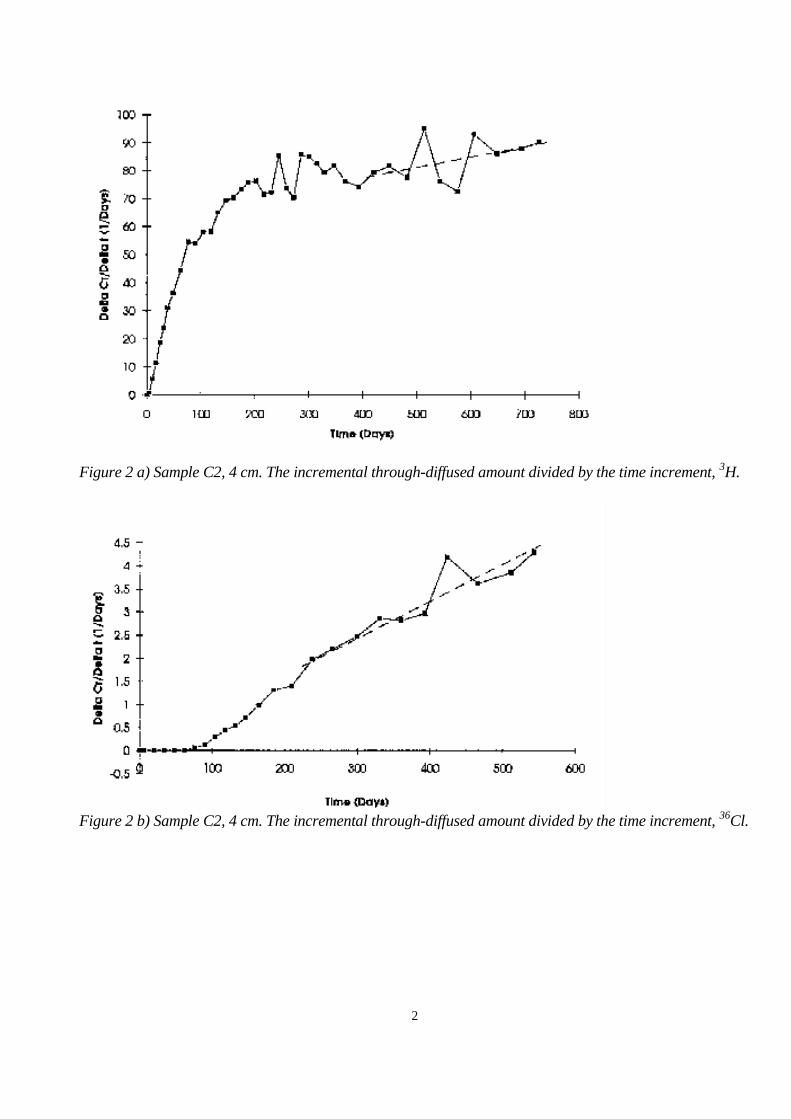
In the following are the graphical presentations of the through-diffused incremental amounts of the tracerdivided by the time increment presented as a function of time together with a line drawn through the lastdata points. The corresponding diffusion coefficient is seen in each figure.
Figure 1 a) Sample C1, 2 cm. The incremental through-diffused amount divided by the time increment, 3H.
Figure 1 b) Sample C1, 2 cm. The incremental through-diffused amount divided by the time increment, 36Cl.
2
Figure 2 a) Sample C2, 4 cm. The incremental through-diffused amount divided by the time increment, 3H.
Figure 2 b) Sample C2, 4 cm. The incremental through-diffused amount divided by the time increment, 36Cl.

3
Figure 3 a) Sample C3, 6 cm. The incremental through-diffused amount divided by the time increment, 3H.
Figure 3 b) Sample C3, 6 cm. The incremental through-diffused amount divided by the time increment, 36Cl.