turbulence, turbulent mixingand diffusion in...

In: Atmospheric Turbulence, Meteorological Modeling... ISBN 978-1-60741-091-1Editors: P. R. Lang and F. S. Lombargo, pp. 167-204 © 2010 Nova Science Publishers, Inc.

Chapter 4

TURBULENCE, TURBULENT MIXING AND DIFFUSION

IN SHALLOW-WATE..-R ESTUARIES

Huhert Chanson l.. and Mark Trevethan2

'The University of Queensland, Brisbane, Australia

2MARUM, The University of Bremen, Germany (formerly Ph.D. graduate in Civil

Engineering. The University of Queensland, Brisbane Australia)

1. INTRODUCTION

In natural waterways and estuaries, an understanding of turbulent mixing is critical to theknowledge of sediment transport, storm-water runoff during flood events, and release ofnutrient-rich wastewater into ecosystems. The predictions of contaminant dispersion inestuaries can rarely be predicted analytically without exhaustive field data for calibration andvalidation. Why? In natural estuaries, the flow Reynolds number is typically within the rangeof 105 to 108 and more. The flow is turbulent, and there is an absence of fundamentalunderstanding of the turbulence structure. Any turbulent flow is characterised by anunpredictable behaviour, a broad spectrum of length and time scales, and its strong mixingproperties. In his classical experiment, Osborne REYNOLDS (1842-1912) illustrated this keyfeature with the rapid mixing of dye of a turbulent flow (REYNOLDS 1883). This is seen inFigure 1 showing the original Reynolds experiment and a modified Reynolds experiment. Inturbulent flows, the fluid particles move in very in'egular paths, causing an exchange ofmomentum from one portion of the fluid to another, as shown in Figure 1 where dye israpidly dispersed in the turbulent flow regime (Re = 2.3 10\ In natural estuaries, strongmomentum exchanges occur and the mixing processes are driven by turbulence. InterestinglyOsborne REYNOLDS himself was involved in the modelling of estuaries (REYNOLDS1887).

Relatively little systematic research was conducted on the turbulence characteristics innatural estuarine systems, in particular in relatively shallow-water systems. Long-duration

* Emai\: [email protected] - Ur\: http://www.uq.edu.aul-e2hchans/ - Ph.: + 6\ 733653516 - Fax: +61733654599

168 Hubert Chanson and Mark Trevethan

studies of turbulent properties at high frequency are extremely limited. Most fieldmeasurements were conducted for short periods, or in bursts, sometimes at low frequency:e.g. BOWDEN and FERGUSON (1980), SHIONO and WEST (1987), KAWANISI andYOKOSI (1994), HAM et al. (2001), VOULGARIS and MEYERS (2004). The data lackedspatial and temporal resolution to gain insights into the characteristics of fine-scaleturbulence. It is believed that the situation derived partly from some limitation with suitableinstrumentation for shallow-water estuaries.

Herein the turbulence characteristics of shallow-water estuaries with semi-diurnal tidesare examined. It is shown that turbulence field measurements must be conducted continuouslyat high frequency for relatively long periods. Detailed field measurements highlight the largefluctuations in all turbulence characteristics during the tidal cycle. While the bulk parametersfluctuate with periods comparable to tidal cycles, the turbulence properties depend upon theinstantaneous local flow properties, and the structure and temporal •.variability of turbulentcharacteristics are influenced by a variety of mechanisms.

Figure 1. Dye dispersion in laminar and turbulent flows (Left) Gravure of the experimental apparatusof Osborne REYNOLDS (1883) (Right) Dye injection in a circular pipe for Re = 3.5 102

, 1.8 103 and2.3 103

Turbulence, Turbulent Mixing and Diffusion in Shallow-Water Estuaries 169

2. TURBULENCE MEASUREMENTS IN SMALL ESTUARIES

2.1. Presentation

Since "turbulence is a three-dimensional time-dependent motion in which vortexstretching causes velocity fluctuations to spread to all wavelengths between a minimumdetermined by viscous forces and a maximum determined by the boundary conditions of theflow" (BRADSHAW 1971, p. 17), turbulence measurements must be conducted at highfrequency to characterise the small eddies and the viscous dissipation process. They must alsoto be performed over a sampling period significantly larger than the characteristic time of thelargest vortical structures to capture the "random" nature of the flow and its deviations fromGaussian statistical properties. Turbulence in natural estuaries is neither homogeneous norisotropic. Basically detailed turbulence measurements are almost impossible in unsteadyestuarine flows unless continuous sampling at high frequency is performed over a full tidalcycle. The estuarine flow conditions and boundary conditions may vary significantly with thefalling or rising tide. In shallow-water estuaries and inlets, the shape of the channel crosssection changes drastically with the tides as shown in Figures 2 and 3. Figures 2 and 3illustrate two sampling sites in a small subtropical estuary at high and low tides. Figure 2presents the cross-section at the mid-estuary sampling site with more than 3 m depth at hightide and less than 0.6 m of water at low tide. Figure 3 shows a narrower section in the upperestuary at both high and low tides.

(A) End of flood tide on 16 May 2005 with poles supporting the instrumentation visible across thecreek.

(B) Low tide on 23 November 2003 - The water depth was less than 0.6 m in the deepest channel nextto the ADY poles during spring tidal conditions.

Figure 2. Sampling site in the mid-estuarine zone of Eprapah Creek, Australia (site 2B, AMTD 2.1 km)looking upstream.


(A) High tide in 28 August 2006 looking downstream (Courtesy ofCIVL4120 student Group 3) - Thewater depth was about 2 m.

(B) Low tide on 8 June 2006 looking upstream (Courtesy ofClive BOOTH).

Figure 3. Sampling site in the upper estuarine zone of Eprapah Creek, Australia (site 3, AMTD 3.1km).

-Turbulence, Turbulent Mixing and Diffusion in Shallow-Water Estuaries 171

All these constraints affect the selection of a suitable, rugged instrumentation for fielddeployment. Traditional propellers and electro-magnetic current meters are adequate for timeaveraged velocity measurements and some large-scale turbulence measurements, but theseinstruments lack temporal and spatial resolution for fine-scale turbulence measurements.Velocity profilers do not work in shallow waters (e.g., less than 0.6 m) while lacking spatialand temporal resolution. A suitable instrumentation for turbulence measurements in shallowwater estuaries is limited to the acoustic Doppler velocimeters (ADV), although the signal canbe adversely affected by "spikes", noises and instabilities.

2.2. Turbulence Properties

Turbulent flows have a great mixing potentia!... involving a wide range of eddy lengthscales (HINZE 1975). Although the turbulence is a "random" process, the small departuresfrom a Gaussian probability distribution constitute some key features. For example, theskewness and kurtosis give some information on the temporal distribution of the turbulentvelocity fluctuation around its mean value. A non-zero skewness indicates some degree oftemporal asymmetry of the turbulent fluctuation: e.g., acceleration versus deceleration, sweepversus ejection. The skewness retains some sign information and it can be used to extractbasic information without ambiguity. An excess kurtosis larger than zero is associated with apeaky signal: e.g., produced by intermittent turbulent events.

In turbulence studies, the measured statistics include usually (a) the spatial distribution ofReynolds stresses, (b) the rates at which the individual Reynolds stresses are produced,destroyed or transported from one point in space to another, (c) the contribution of differentsizes of eddy to the Reynolds stresses, and (d) the contribution of different sizes of eddy tothe rates mentioned in (b) and to rate at which Reynolds stresses are transferred from onerange of eddy size to another (BRADSHAW 1971). The Reynolds stress is a transport effectresulting from turbulent motion induced by velocity fluctuations with its subsequent increaseof momentum exchange and of mixing (PIQUET 1999). The turbulent transport is a propertyof the flow. The turbulent stress tensor, or Reynolds stress tensor, includes the normal andtangential stresses, although there is no fundamental difference between normal stress and

tangential stress. For example, (vx+vy)/ J2 is the component of the velocity fluctuation along

a line in the xy-plane at 45° to the x-axis; hence its mean square (v x2 + v Y2 + 2 v xv y ) / 2 is

the component of the normal stress over the density in this direction although it is acombination of normal and tangential stresses in the x- and y-axes.

2.3. Field Experiments in Shallow-Water Estuaries with Semi-Diurnal Tides

A series of detailed turbulence field measurements were conducted in two shallow-waterestuaries with a semi-diurnal tidal regime (Table 1).

In Hubert Chanson and Mark Trevethan

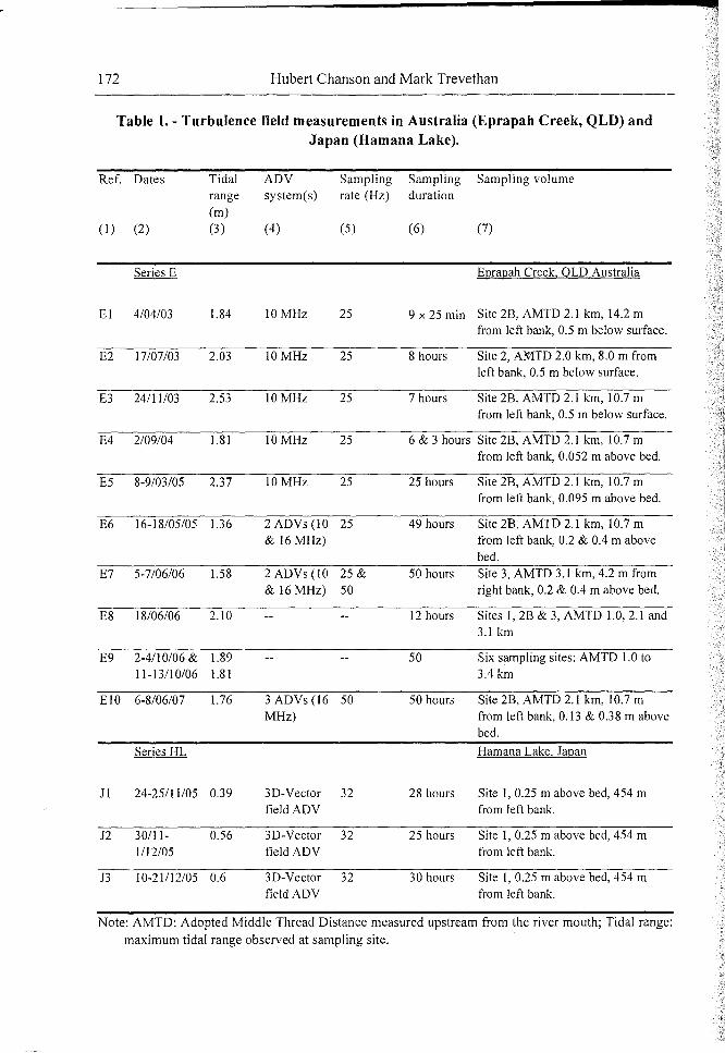
Table 1. - Turbulence field measurements in Australia (Eprapah Creek, QLD) andJapan (Hamana Lake).

Ref. Dates Tidal ADV Sampling Sampling Sampling volumerange system(s) rate (Hz) duration(m)

(I) (2) (3 ) (4) (5) (6) (7)

Series E Eprapah Creek. QLD Australia

El 4/04/03 1.84 10MHz 25 9 x 25 min Site 2B, AMTD 2.1 km, 14.2 mfrom left bank, 0.5 m below surface.

E2 17/07/03 2.03 IOMHz 25 8 hours Site 2, A~TD 2.0 km, 8.0 m fromleft bank, 0.5 m below surface.

E3 24/11/03 2.53 IOMHz 25 7 hours Site 2B, AMTD 2.1 km, 10.7 mfrom left bank, 0.5 m below surface.

E4 2/09/04 1.81 10MHz 25 6 & 3 hours Site 2B, AMTD 2.1 km, 10.7 mfrom left bank, 0.052 m above bed.

E5 8-9/03/05 2.37 10MHz 25 25 hours Site 2B, AMTD 2.1 km, 10.7 mfrom left bank, 0.095 m above bed.

E6 16-18/05/05 1.36 2 ADVs (10 25 49 hours Site 2B, AMTD 2.1 km, 10.7 m& 16 MHz) from left bank, 0.2 & 0.4 m above

bed.

E7 5-7/06/06 1.58 2 ADVs (10 25 & 50 hours Site 3, AMTD 3.1 km, 4.2 m from& 16 MHz) 50 right bank, 0.2 & 0.4 m above bed.

E8 18/06/06 2.10 12 hours Sites I, 2B & 3, AMTD 1.0, 2.1 and3.1 km

E9 2-4/10/06 & 1.89 50 Six sampling sites: AMTD 1.0 to11-13/10/06 1.81 3.4 km

EIO 6-8/06/07 1.76 3 ADVs (16 50 50 hours Site 2B, AMTD 2.1 km, 10.7 mMHz) from left bank, 0.13 & 0.38 m above

bed.

Series HL Hamana Lake. Japan

Jl 24-25/11/05 0.39 3D-Vector 32 28 hours Site I, 0.25 m above bed, 454 mfield ADV from left bank.

J2 30/11- 0.56 3D-Vector 32 25 hours Site 1,0.25 m above bed, 454 m

1/12/05 field ADV from left bank.

13 10-21/12/05 0.6 3D-Vector 32 30 hours Site I, 0.25 m above bed, 454 mfield ADV from left bank.

Note: AMTD: Adopted Middle Thread Distance measured upstream from the river mouth; Tidal range:

maximum tidal range observed at sampling site.


At Eprapah Creek (Australia), the estuarine zone was 3.8 km long, about 1 to 2 m deepmid-stream (Fig. 2 & 3). This was a relatively small estuary with a narrow, elongated andmeandering channel (CHANSON et al. 2005, TREVETHAN et al. 2007a, 2008). It is adrowned river valley (coastal plain) type with a small, sporadic freshwater inflow, a crosssection which deepens and widens towards the mouth, and surrounded by extensive mud flats.This type of estuary is very common in Australia. It is also called an alluvial estuary(SAVENUE 2005) and can be classified as a wet and dry tropical/subtropical estuary(DlGBY et al. 1999). Although the tides are semi-diurnal, the tidal cycles have slightlydifferent periods and amplitudes indicating that a diurnal inequality exists. Table 1summarises ten field studies conducted between 2003 and 2007. A range of field conditionswere tested: tidal conditions from neap tides (Studies E6, E7, EI0) to spring tides (StudiesE3, E5, E8), and different bathymetry from mid-estuary (Studies E5, E6, El 0) to upperestuary (Study E7) (Table 1). ,.r

Another series of field studies were undertaken at Hamana Lake, Japan in late 2005(TREVETHAN 2008). Hamana Lake is a relatively large tidal lake with a small opening tothe Pacific Ocean (Fig. 4). It extends approximately 15 km inland and has a surface area of7.4 107 m2

• The width of the entrance is approximately 200 m and is controlled by man madestructures (Fig. 4A). The depth of Hamana Lake increases landwards, from less than 1 m nearthe entrance to more than 12 m further inland. The field investigations were conducted underneap and spring tidal forcing, collecting continuous high frequency turbulence data over a 25hour period. The sampling site was located in a shallow area near the estuary mouth (Fig. 4).This type of shallow region is typical of restricted entrance (bar-built) type estuaries (DYER1997). It was located approximately 600 m North-East of the main navigation channel, 450 mSouth of the nearest bank and approximately 3.5 km NNW of the estuary mouth seen inFigure 4A. The mean depth was approximately 0.9 m during the two field studies and themaximum tidal range during the field studies were 0.39 and 0.56 m.

(A) Estuary mouth in 1999 (Courtesy ofMr. KATO, Omotehama network).

Figure 4. (Continued)


(B) Hamana Lake sampling site on 24 November 2005, looking North to nearest bank about 450 maway.

(C) Wind waves on 24 November 2005 with the poles holding the ADV system on the far left.

Figure 4. Photographs of Hamana Lake (Japan).


2.4. Instrumentation

Turbulent velocities were measured with acoustic Doppler velocimetry. That is, aSontek™ UW 3D ADV (10 MHz) and some Sontek™ 20 micro-ADV (16 MHz) in Australia(Eprapah Creek), and a Nortek™ 3D-Vector field ADV in Japan (Hamana Lake). Theturbulent velocity measurements were performed continuously at high frequency for between8 to 50 hours during various tide conditions (Table 1, columns 5 & 6). All ADV units weresynchronised carefully within 20 ms for the entire duration of the studies.

The acoustic backscatter intensity of some ADV signals was also analysed. Thebackscatter intensity is a function of the ADV signal amplitude that is proportional to thenumber of particles within the sampling volume:

(1)

where the backscatter intensity Ib is dimensionless and the average amplitude Ampl is incounts. (The coefficient 10-5 is a value introduced to avoid large values of backscatterintensity.) The backscatter intensity may be used as a proxy for the instantaneous suspendedsediment concentration (SSC) within the sampling volume because of the strong relationshipbetween Ib and SSC (THORNE et al. 1991, FUGATE and FRIEDRICHS 2002, CHANSONet al. 2008a). The terms Vxh is proportional to the suspended sediment flux per unit area,where Vxis the longitudinal velocity component.

A thorough post-processing technique was developed and applied to remove electronicnoise, physical disturbances and Doppler effects (CHANSON et al. 2008b). The fieldexperience demonstrated that the gross ADV signals were unsuitable, and led often toinaccurate time-averaged flow properties and turbulent characteristics. Herein only postprocessed data are discussed.

2.5. Calculations of Turbulence Properties

The post-processed data sets included the three instantaneous velocity components Vx, Vy

and Vz, and the backscatter intensity Ib, where x is the longitudinal direction positivedownstream, y is the transverse direction positive towards the left bank and z is the vertical

direction positive upwards. The turbulent fluctuations were defined as : v = V - V and

i b =I b - I b , where V vyas the instantaneous (measured) velocity component, V was the

variable-interval time average (VITA) velocity and I b was the VITA backscatter intensity. A

cut-off frequency was selected with an averaging time greater than the characteristic period ofturbulent fluctuations, and smaller than the characteristic period for the time-evolution of themean tidal properties. An upper limit of the filtered signal was the Nyquist frequency. Theselection of the cut-off frequency was derived from a sensitivity analysis (CHANSON et al.2008b, TREVETHAN 2008). Herein all turbulence data, including the turbulent flux events,were processed using samples that contain 5,000 to 10,000 data points and calculated every10 s along the entire data sets. In a study of boundary layer flows, FRANSSON et al. (2005)proposed a cut-off frequency that was consistent with the selected sample size.


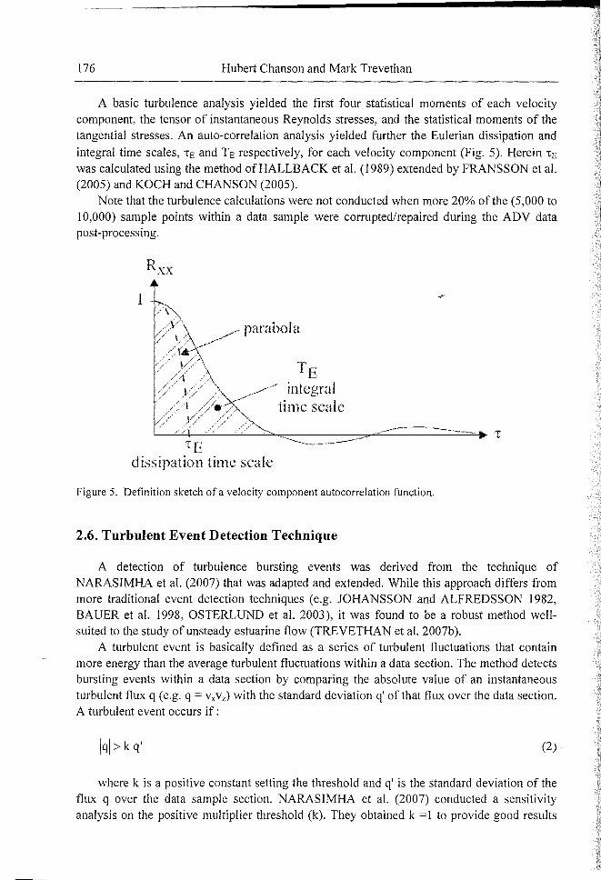
A basic turbulence analysis yielded the first four statistical moments of each velocitycomponent, the tensor of instantaneous Reynolds stresses, and the statistical moments of thetangential stresses. An auto-correlation analysis yielded further the Eulerian dissipation and

integral time scales, LE and TE respectively, for each velocity component (Fig. 5). Herein LEwas calculated using the method of HALLBACK et al. (1989) extended by FRANSSON et al.(2005) and KOCH and CHANSON (2005).

Note that the turbulence calculations were not conducted when more 20% of the (5,000 to10,000) sample points within a data sample were corrupted/repaired during the ADV datapost-processing.

R>XX

I

parabola

'rEintegral

time scale

T'rE

dissipation time scale

Figure 5. Definition sketch of a velocity component autocorrelation function.

2.6. Turbulent Event Detection Technique

A detection of turbulence bursting events was derived from the technique ofNARASIMHA et al. (2007) that was adapted and extended. While this approach differs frommore traditional event detection techniques (e.g. JOHANSSON and ALFREDSSON 1982,BAUER et aI. 1998, OSTERLUND et al. 2003), it was found to be a robust method wellsuited to the study of unsteady estuarine flow (TREVETHAN et aI. 2007b).

A turbulent event is basically defined as a series of turbulent fluctuations that containmore energy than the average turbulent fluctuations within a data section. The method detectsbursting events within a data section by comparing the absolute value of an instantaneousturbulent flux q (e.g. q = vxvz) with the standard deviation q' of that flux over the data section.A turbulent event occurs if:

Iql>kq' (2)

where k is a positive constant setting the threshold and q' is the standard deviation of theflux q over the data sample section. NARASIMHA et aI. (2007) conducted a sensitivityanalysis on the positive multiplier threshold (k). They obtained k =1 to provide good results


in atmospheric boundary layer studies and a similar result was obtained in an estuarine system(TREVETHAN et al. 2007b). Herein k = 1 and consecutive data sections of 10,000 datasample points (200 s at 50 Hz) were used.

For each data section, the information of each detected event encompassed the eventstart/finish times, duration L, dimensionless flux amplitude A and relative magnitude m. Theevent properties were used to compare individual turbulent events within a data set andbetween synchronised data sets collected simultaneously. Figure 6A introduces the definition

of the duration and amplitude of an isolated event. The duration L of the event is the timeinterval between the "zeroes" in momentum flux (e.g. q = vxvz) nearest to the sequence ofdata points satisfying Equation (2) (Fig. 6A). Practically, the event duration is calculated fromthe first data point with the same sign as the event to the first data point after the change insign in momentum flux. The method provides an accurate estimate of the event durationwithin the limitations of the sampling frequency. Tile dimensionless amplitude A of an eventis the ratio of the averaged flux amplitude during the event to the long-term mean flux of theentire data section:

1 " qA== f -dt

q t=O L

(3)

-where q is the averaged value of q over the data section, L is the event duration and dt =

l/fscan (e.g. f scan = 50 Hz). The relative contribution of an event to the total momentum flux

of the data section is called the relative magnitude m defined as:

ALm=-

T(4)

where T is the total duration of the data section : i.e., T = 200 s for 10,000 samplescollected at 50 Hz. This technique was applied to the momentum fluxes vxvy and VxVz, and tothe "pseudo" longitudinal suspended sediment flux vxib, where ib is the instantaneousfluctuation in the ADV backscatter intensity.

The method was extended to investigate turbulent sub-events within a large event. Forexample, in Figure 6A, the turbulent event is characterised by three distinct peaks inmomentum flux and the entire event may be represented as a succession of three consecutive"turbulent sub-events". The second sub-event is highlighted with hatching in Figure 6B. Aturbulent sub-event was defined when the instantaneous momentum flux within the mainturbulent event was greater than the momentum flux threshold (Eq. (2)) of the data section. InFigure 6B, the definition of duration and amplitude of the sub-event are shown. For each subevent, its start/finish times, duration, dimensionless flux amplitude and relative magnitudewere calculated within a given event. The duration of a sub-event is that time interval duringwhich the momentum flux was equal to or greater than the threshold value. For each subevent, the dimensionless sub-event amplitude is the ratio of the averaged sub-event amplitudeto the sub-event duration to the mean flux over the data section. The sub-event propertieswere calculated for consecutive data sections containing 10,000 data points (200 s at 50 Hz)


along each data set with the same technique used to analyse turbulence events, including thenumber of sub-events that occurred in each individual event.

Sample average vxvz

Event amplitude

rvxvz dto

,~ _-_._-_.._._.+!

Event dumtion 1:

Sample threshold (vxvz)'

----L---------r~-r~-h~

4

::.

()+--+----\----+---::>~-__I__t_------+____----_+__f<_+----"'-<-...-_4__+_.

!, !lnstantaneous VxVz (m~!s"')

31831 31831.2

Time (s) sinee 00:00 on 6/6/07

31831.4

(A) Definition sketch of flux event and event parameters.

Sub-evenl amplitude

-2

Sample threshold (vxvzr

____l _

i-t - - _ :

Event duration T

3183l 31831.2 31831.4

Time (s) since 00:00 on 6!6/07

(B) Definition sketch of turbulent sub-events within a turbulent event.

Figure 6. Turbulent flux event definitions and momentum flux data in terms ofvxvz (study ElO,Eprapah Creek, data collected at 0.38 m above bed).


3. TURBULENT FLOW PROPERTIES AT THE MACROSCOPIC SCALES:

BASIC PATTERNS

3.1. Basic Flow Properties

The estuarine flow was an unsteady process. The bulk parameters including the waterdepth and time-average longitudinal velocity were time-dependant and they fluctuate withperiods comparable to tidal cycles and other large-scale processes. This is illustrated inFigures 7 and 8 showing the water depth, water conductivity and time-averaged velocitiesrecorded mid-estuary for two field studies in Australia (Eprapah Creek). Figure 7 presents thewater depth and conductivity data recorded about mid-estuary during neap tide conditions.The results highlighted some tidal asymmetry during a 24 hours 50 minutes period with asmaller (minor) tidal cycle followed by a larger (major) tidal amplitude. The waterconductivity variations were driven primarily by the ebb and flood tides. The moderate rangeof specific conductivity seen in Figure 7 was typical of a small subtropical estuary under neaptidal conditions in absence of freshwater runoff.

51.6

50.4

49.2 E~Cl)

48 E-o

46.8:~u:l"0

45.6§"~"'"44.4 ~

'6 43.2

Study E6o Water depth

--~d",ti~'Y P'lf\t

2

1.2

2.2

1.4

1.8

0 0 8<{,

\;OJ 4230000 50000 70000 90000 110000 130000 150000 170000 190000 210000

Time (s) since 00:00 on 16/0512005

Figure 7. Time variations of the water depth and conductivity in the mid-estuary zone of Eprapah Creek(Australia) during neap tide conditions (study E6).

Figures 8 and 9 present the time-averaged longitudinal velocities in Australia (Fig. 8) andin Japan (Fig. 9). Figure 8 shows data collected in the middle of the deepest channel duringspring and neap tides. For all mid-estuary field studies, the largest velocity magnitudeoccurred just before and after the low tide, with the flood velocities always larger than ebbvelocities. KAWANISI and YOKOSI (1994) observed similarly maximum flood and ebbvelocities around low tide and larger flood velocities, during some field works in an estuarinechannel in Japan. The velocity data showed some multiple flow reversal events around hightides and some long-period oscillations in water elevation and velocity around mid-tide.Figure 8A shows an example of long-period velocity oscillations during the flood tidebetween t = 105,000 and 125,000 s where the time t is counted since midnight (00:00) on thefirst day of the study. Figure 8B presents an illustration of multiple flow reversals about high


tide between t = 50,000 and 65,000 s. These low frequency velocity oscillations were possiblygenerated by some resonance caused by the tidal forcing interacting with the estuarytopography and the outer bay system (CHANSON 2003, TREVETHAN 2008). These effectswere more noticeable during neap tide conditions and seemed more pronounced in the upperestuary (TREVETHAN et al. 2007a).

At Hamana Lake, the tidal range was small during both spring and neap tidal conditionsbecause the restricted entrance (Fig. 4C) reduced the tidal range observed in the estuary bydampening the ocean tidal oscillations. The difference in tidal range was less than 0.2 mbetween neap and spring tide studies (Fig. 9). The response of the time-averaged streamwisevelocity to the tidal forcing was different between Eprapah Creek and Hamana Lake. Figure 9shows the time-averaged streamwise velocity and water depth as functions of time in Japan.The maximum flood and ebb velocities at Hamana Lake were observed in the middle of thetide under spring and neap tidal forcing. HAM et al. (2001) observed a similar tidal trend in a

.;;--

shallow semi-enclosed bay. During neap tidal conditions, the maximum flood and ebbvelocity suggested a neutral tidal bias (Fig. 9B). However, under spring tidal forcing, themaximum ebb velocity at Hamana Lake was larger than the maximum flood velocity (Fig.9A).

(A) Longitudinal velocity data collected at 0.1 m above the bed during spring tides (study E5).

(B) Longitudinal velocity data collected at 0.4 m above the bed during neap tides (study E6).

Figure 8. Time variations of the time-averaged longitudinal velocity Vx (positive downstream) and

water depth for a full tidal cycle at Eprapah Creek (Australia), mid-estuary zone (site 2B) - Legend: [] time-averaged longitudinal velocity (cm/s); [] water depth.


50000 60000 70000 80000 90000time (s) since 00:00 on 3011112005

100000 110000

(A) Longitudinal velocity data collected at 0.25 m above the bed during spring tides (study 12).

70000 80000 90000 100000 110000time (s) since 00:00 on 2411112005

120000 130000

(B) Longitudinal velocity data collected at 0.25 m above the bed during neap tides (study 11).

Figure 9. Time variations of the time-averaged longitudinal velocity Vx (positive downstream) and

water depth for a full tidal cycle at Hamana Lake (Japan) - Legend: [-] time-averaged longitudinalvelocity (cm/s); [] water depth.

3.2. Turbulence Properties

The field observations showed systematically large standard deviations of all velocitycomponents at the beginning of the flood tide for all tidal cycles. Typical field measurementsof standard deviations for the longitudinal velocity vx' are shown in Figure 10 for two tidalcycles in spring and neap tides in Australia and Japan. Figure 10 shows the magnitude of vx'

from a low water (LW I) to the next low water (LW2), and the data are presented in a circularplot. In such a circular plot, the radial coordinate is the turbulent property vx' and the angularcoordinate is the time relative to the next low water. From the first low water, the timevariations of the data progress anticlockwise until the next low water. The high and lowwaters are indicated: the low waters are the positive horizontal axis, and the high waters arethe dotted lines. The upper half of the graph corresponds roughly to the flood tide while thelower half represents the ebb tide.

In Australia, the standard deviations of all velocity components were two to four timeslarger in spring tides than during neap tides. Figure lOA highlights the large velocity standarddeviations in spring tide conditions. The presentation illustrates that vx ' was systematicallylarger during the flood tide than during the ebb tide, while there were significant fluctuations


in velocity standard deviations during the entire tidal cycle. KAWANISI and YOKOSI (1994)observed similarly larger measured velocity standard deviations during flood tide in a large

tidal channel.

At Hamana Lake, the tidal trends of all velocity standard deviations were about the samefor spring and neap tidal conditions, but the median values were twice as large during springtides (Fig. lOB). The observation tended to indicate that the largest velocity standard

deviations occurred about the time of maximum longitudinal velocity as noted inTREVETHAN (2008).

-6

(A) Eprapah Creek (Australia), mid-estuary zone (site 2B), study E5 (0.1 m above bed), and study E6(0.4 m above bed).

JIBW

(B) Hamana Lake (Japan).

·6

J21!\V

·4

·6 -

LWI

L\V2

Figure 10. Time variations of the standard deviations of the longitudinal velocity vx' (cm/s) during amajor tidal cycle in spring and neap tidal conditions: [e] spring tide, and ['] neap tide - Circular plotfrom a low water to the next low water - Dotted line: high water.

The horizontal turbulence intensity vy'/vx ' was approximately equal to 1 for spring andneap tide conditions at both Eprapah Creek and Hamana Lake, indicating that turbulence

fluctuations in the longitudinal and transverse directions were of similar magnitude. Theywere larger than laboratory observations in straight prismatic rectangular channels which

yielded vy'/vx' = 0.5 to 0.7 (NEZU and NAKAGAWA 1993, KOCH and CHANSON 2005),


but the findings were close to recent LES computations in a shallow water channel withsimilar Reynolds number conditions (HINTERBERGER et al. 2008). The vertical turbulenceintensities vz'/vx ' were similar to the observations of SHI0NO and WEST (1987) andKAWANISI and YOKOSI (1994) in estuaries, and ofNEZU and NAKAGAWA (1993) andXIE (1998) in laboratory open channels. For all estuarine studies in Australia and Japan,vz'/vx' was always smaller than the horizontal turbulence intensity vy'/vx' and the result impliedsome form of turbulence anisotropy.

The skewness and kurtosis gave some information on the temporal distribution of theturbulent velocity fluctuation around its mean value. For all studies, the skewness andkurtosis of all velocity components fluctuated significantly during each tidal cycle. Theyexhibited some characteristics that differed from the expected skewness and kurtosis for aGaussian distribution. The normalised third (skewness) and fourth (kurtosis) moments of thevelocity fluctuations appeared to be close to the obsyrvations of SHIONO and WEST (1987)in an estuary. They were also comparable with the LDV data ofNIEDERSCHULTZE (1989)and TACHIE (2001) in developing turbulent boundary layers in laboratory channels.

All tangential Reynolds stresses showed significant fluctuations over the tidal cycles of

all field studies undertaken at both estuaries. The turbulent stress p v x V z close to the bed

varied with the tides, being predominantly positive during the flood tide and negative duringthe ebb tide. This trend was consistent with the earlier data of OSONPHASOP (1983),KAWANISI and YOKOSI (1994) and HAM et al. (2001) in tidal channels. The negative

correlation between p v x Vz and Vx was also consistent with traditional boundary layer

results (XIE 1998, TACHIE 2001, NEZU 2005). At Eprapah Creek the magnitudes of alltangential Reynolds stresses were at least an order of magnitude larger during spring tidesthan those observed for neap tidal conditions. The larger magnitude of all Reynolds stressesderived from the increased tidal forcing interacting with the local bathymetry. However, atHamana Lake, the difference in the magnitude of all Reynolds stresses under spring and neaptidal forcing was not as significant, with Reynolds stress magnitudes being up to twice aslarge under spring tidal forcing. The smaller difference in spring and neap turbulent stressmagnitudes at Hamana Lake was conceivably related to the small difference in tidalamplitude between the field investigations (Table I).

The standard deviations of all tangential Reynolds stresses increased with increasinglongitudinal velocity magnitude. At Eprapah Creek (Australia), the magnitude of alltangential Reynolds stress standard deviations were one order of magnitude greater underspring tidal forcing than those observed during neap tides. At Hamana Lake (Japan), thespring tidal tangential Reynolds stress standard deviations were approximately twice as largeas those measured under neap tidal conditions. The results obtained in both estuaries showedthat the probability distribution functions of all tangential Reynolds stresses were notGaussian.

3.3. Turbulence Time Scales

The integral time scale of a velocity component is a measure of the longest connection inthe turbulent behaviour of that velocity component. Some variations of longitudinal integraltime scales TEx are shown in Figure 11 for a major tidal cycle during neap and spring tide


conditions. Note that the axes have a logarithmic scale and the units are milliseconds. AtEprapah Creek significant fluctuations in the horizontal integral time scales were observedthroughout the tidal cycles, with the integral time scales observed under neap tidal conditionsbeing larger than those for spring tides (Figure 11). The horizontal integral times at EprapahCreek ranged between 0.06 sand 1.0 s with a median value of approximately 0.15 sunderspring tides and between 0.06 sand 2.40 s (median value: 0.31 s) during neap tidalconditions. In Hamana Lake, the fluctuations in horizontal integral time scales over the tidalcycle were relatively small. The horizontal integral time scales ranged between 0.2 sand 1.5 sunder both spring and neap tides (Figure 11). The median values of longitudinal andtransverse integral time scales at Hamana Lake were approximately 0.75 a and 0.58 sunderspring and neap tidal conditions respectively.

ESHY::


-4

(B) Hamana Lake (Japan), 0.28 m above the bed.

Figure 11. - Time variations of the integral time scale TEx (units: ms) for Vx during a major tidal cyclefor neap and spring tidal conditions - The axes have a logarithmic scale - Legend: [.] spring tide; [']neap tide.

ps



(B) Hamana Lake (Japan), 0.28 m above the bed.

Figure 12. Time variations of the dissipation time scale LEx (units f..ls) for Vx during a major tidal cyclefor neap and spring tidal conditions - The axes have a logarithmic scale - Legend: [.] spring tide; [~]

neap tide.

The dissipation time scale, also called Taylor micro scale, is a measure of the most rapidchanges that occur in the fluctuations of a velocity component. It is a characteristic time scaleof the smaller eddies which are primary responsible for the dissipation of energy. Figure 12

shows the variations of longitudinal dissipation time scales 'Ex for a major tidal cycle duringneap and spring tide conditions in Australia and in Japan. The axes have a logarithmic scale


and the units are in microseconds. At both estuaries, the dissipation time scale data seemedindependent of the tidal phase with horizontal dissipation time scales between 0.0001 sand0.03 s for all field studies (Fig. 12). The dissipation time scales at Eprapah Creek seemedindependent of the tidal conditions, vertical and longitudinal sampling locations, with medianvalues typically between 0.002 sand 0.003 s. At Hamana Lake, the median values of the

horizontal dissipation time scales (LEx and LEy) were between 0.007 sand 0.011 s for spring

tidal conditions, and between 0.004 sand 0.006 s during neap tidal conditions. The horizontaldissipation time scales were slightly different, and the median values of transverse dissipation

time scales LEy were larger than the median values of longitudinal dissipation time scales

LEx under spring and neap tidal forcing. Note that the dissipation time scales were

consistently smaller than the time between two consecutive samples: e.g., l/fscan = 0.04 s forfscan = 25 Hz in Figure 12. The findings highlighted that a high frequenty sampling is requiredand the sampling rates must be at least 20 to 30 Hz to capture a range of eddy time scalesrelevant to the dissipation processes.

The analysis of the integral and dissipation time scales of all velocity componentsshowed no obvious trend with tidal phase under both neap and spring tidal forcing. Duringthe present field studies at Hamana Lake and Eprapah Creek, the dimensionless transverseand vertical dissipation time scales were respectively: TEylTEx ~ 1 and TElTEx ~ 1 to 3. In atidal channel in Southern Australia, OSONPHASOP (1983) observed TEylTEx ~ 1.7 andTEz/TEx ~ 2.2.

3.4. Dimensionless Turbulence Parameters

For most turbulence properties, the spring tidal data at Eprapah Creek were larger andshowed a more asymmetrical tidal response. For example, the standard deviations oflongitudinal velocity under spring tidal conditions were larger at Eprapah Creek than atHamana Lake, despite the larger longitudinal velocity observed at Hamana Lake (Fig. 8, 9and 10). The ratio of local tidal amplitude and local mean depth at the experimental site al/hlmay assist with the understanding of this phenomenon (TREVETHAN 2008).

Dimensionless turbulence parameters are commonly used in turbulence investigations tocompare the relative turbulence characteristics of different systems under distinct flowconditions. Table 2 regroups the median values of basic dimensionless turbulence properties inAustralia and Japan. The dimensionless turbulence parameters include the turbulent intensityratios (vy'/vx', v//vx'), the relative turbulence intensities of the longitudinal, transverse and

vertical velocity fluctuations (V~/IVx I, v~ /IVxI, v~/IVx I), the:ormalized tangential

Reynolds stresses (IVxVz1/Vx2, Ivxv y1/Vx2 , Ivy v z1/Vx2 ), the magnitude of correlation

coefficients of Reynolds stresses (IR vxvz I, IR vxvy I, IR,yvz I) and the dimensionless integral

time scales (TEx~g/hl ' TEy~g/hl ' TEz~g/hl ).


Table 2. Median values of dimensionless turbulence parameters over the fullinvestigation periods for the field studies undertaken in Australia (Eprapah Creek) and

Japan (Hamana Lake).

Estuary Eprapah Creek Hamana Lake

Field Study I E5I

E6 Jl J2I

Tidal Conditions Spring Neap Neap Spring

Tidal range (m) 2.37I

1.36 0.39 0.56

a/hI 0.76 0.43 0.22 0.31

v 'Iv ' I1.00 0.89 0.83 0.86y x

vz'Ivx' 0.39 0.51 0.52 0.56

vx'/jvx I 0.42 0.21 0.15 0.13

vy'/IVx I 0.44 0.19 0.15 0.13

Vx'/IVx I 0.16 0.11 0.07 0.07

Ivxvzl/Vx2

I0.014 0.005 0.004 0.004

Ivxv yl/Vx2

0.014 0.004 0.003 0.002

Ivyv zl/Vx2

0.004 0.002 0.001 0.001

IRvxvyl 0.08

I0.13 0.20 0.27

IR vxvz I 0.23 0.17 0.31 0.30

IRvyvz II

0.07 0.10 0.13 0.20

TEx~g/hl 0.43 0.59 2.45 2.50

TEy~g/hl 0.30 0.93 1.86 1.94

TEz~g/hl 0.72 2.06 1.98 1.39

The dimensionless turbulence data suggested a different set of turbulence and mixingproperties when aI/hI> 0.5 (Table 2), while the magnitudes of relative turbulence intensitiesand normalised Reynolds stresses were similar for aI/hI < 0.5. Previous turbulence studies in


large estuarine systems (e.g. BOWDEN and HOWE 1963, OSONPHASOP 1983, WEST and

ODUYEMI 1989) yielded results of </IVxl < 0.15 and IVxVzl/Vx2 < 0.004, that were

similar to those observed at Hamana Lake and Eprapah Creek when al/h l < 0.5. The findingsindicated that the turbulence properties of estuaries with al/h l < 0.5 could not be applied toshallow-water estuaries where al/hl > 0.5.

3.5. Suspended Sediment Fluxes

For some field studies in Australia (Eprapah Creek), an acoustic Doppler velocimeter(ADV) was calibrated in terms of the backscatter intensity versus suspended sedimentconcentration (SSC) (CHANSON et al. 2008a). The results enabled archaracterisation of thefluctuations in suspended sediment concentrations for two field studies (E6 and E7).

The instantaneous suspended sediment concentration (SSC) showed some largefluctuations throughout the entire field studies, including during the tidal slacks (high and lowtides). The data tended to indicate larger suspended loads during the early flood tides. Thedata showed also some low frequency oscillation patterns in terms of the SSC that may belinked with the low frequency fluctuations of the streamwise velocity. In the middle and

upper estuarine zones, the ratio SSC'l SSC was respectively 0.66 and 0.57 on average, where

SSC is the time-averaged suspended sediment concentration and SSC' is its standarddeviation.

The instantaneous advective suspended sediment flux per unit area qs was calculated as :

(5)

where qs and Vx are positive in the downstream direction, and the suspended sedimentconcentration SSC is in kg/m3

• qs is a local measure of the suspended sediment flux at theADV sampling site. Typical instantaneous suspended sediment flux per unit area results arepresented in Figure 13. The data characterise the advective suspended sediment flux per unitarea in a sampling volume located at 0.2 m above the bed.

The sediment flux per unit area data showed typically an upstream, negative suspendedsediment flux during the flood tide and a downstream, positive suspended sediment fluxduring the ebb tide. The instantaneous suspended sediment flux per unit area data qs showedconsiderable time-fluctuations that derived from a combination of velocity and suspendedsediment concentration fluctuations. The data demonstrated further some high frequencyfluctuation with some form of suspended sediment flux bursts that were likely linked to andcaused by some turbulent bursting phenomena next to the bed. Some low frequencyfluctuations in suspended sediment flux were also observed. In the middle estuary, themagnitude of suspended sediment fluxes were about one order of magnitude larger than thoseobserved in the upper estuary.

For each tidal period of 24 hour 50 min., the suspended sediment flux per unit area datawere integrated with respect of time. The results gave the net sediment mass transfer per unitarea at the sampling volume:


ills = fqs clt (6)

24h50min

For both field studies E6 and E7, the net sediment mass transfer per area was negative(i.e. upstream). In the middle estuary, Equation (6) yielded ms = -22.3 and -20.8 kg/m2 foreach 24 h 50 min tidal period, while Equation (6) gave ms = -6.66 and -1.81 kg/m2 in theupper estuary. That is, the net sediment flux over a full tidal cycle corresponded on average toan upstream net suspended sediment transfer. Several researchers investigated the netsuspended sediment flux in estuaries of subtropical and tropical river estuaries during similardry conditions and tidal ranges. Previous results showed a similar net upstream sedimenttransfer in dry weather: e.g., LARCOMBES and RIDD (1992), HOSSAIN et al. (200 I),KAWANISI et al. (2006). However, during rain storms and wet weather the net sedimentmass flux is positive in the downstream direction in-such estuarine systems.

A striking feature of the analysed data sets is the large fluctuations in the suspendedsediment fluxes during the tidal cycles. This feature was rarely documented, but an importantfeature of the data sets is that the present data were collected continuously at high frequency(25 and 50 Hz) during relatively long periods. It is however acknowledged that the data werepoint measurements. Any extrapolation would imply that the sampling volume wasrepresentative of the entire channel cross-section.

.., \,,,

Study £6 (z = 0.2 ill)--' SSCxV. (kg/s/m})• - - - "Vater depth (m)0.024

1-r..----~_-...I

0.016

0.008

0.032

-0.024

-0.032

-0.016

>{

>w -0.008v;II""

-0.04 0.5630000 50000 70000 90000 noooo 130000 150000 170000 190000 210000

Time (s),mce 00:00 Oll 16"05/2005

Figure 13. Time variations of the instantaneous suspended sediment flux per unit surface area (SSCxV"positive downstream) and measured water depth during the study E6 (neap tide) at 0.2 m above bed.

The integral time scale of the suspended sediment concentration (SSC) data represents acharacteristic time of turbid suspensions in the creek. Calculations were performed for twofield studies in Australia (E6 and E7). The SSC integral time scale data seemed relativelyindependent of the tidal phase and yielded median SSC integral time scales TEsse of about0.06 s.


A comparison between the turbulent and SSC integral time scales showed somedifference especially during the ebb tide. In the mid-estuarine zone, the ratio of SSC toturbulent integral time scales was on average TEssdTEx = 0.21 and 0.14 during the flood andebb tides respectively. In the upper estuary, the ratio TEssdTEx was about TEssc/TEx = 1 and0.18 during the flood and ebb tides respectively. Basically the ratio TEssc/TEx was about 2 to 5times lower during ebb tide periods. The findings tended to suggest that the sedimentsuspension and suspended sediment fluxes were dominated by the turbulent processes duringthe flood tide, but not during the ebb tide. The experimental results showed further somefluctuations in SSC integral time scales during the tidal cycle.

These data sets provided simultaneous turbulence and suspended sediment concentrationmeasurements recorded continuously at high frequency for 50 hours per investigation. Thedata analyses yielded an unique characterisation of the turbulent mixing processes andsuspended sediment fluxes. The integral time scales for turbulence ~md suspended sedimentconcentration were about equal during flood tides, but differed significantly during ebb tides.The same pattern might take place with other scalars and be pertinent to the turbulent mixingmodelling in shallow-water subtropical estuaries under dry-weather conditions.

3.6. Discussion

The boundary shear stress may be estimated from the velocity gradient next to the bed,although other techniques may be used (SCHLICHTING 1979, MONTES 1998, KOCH andCHANSON 2005). The near-bed velocity shear stress is calculated as:

.0 =p[K (vx),]' (7)

Lzl

n-k s

where p is the fluid density, (Vx)1 is the time-averaged longitudinal velocity of the ADV

unit located closest to the bed (ZI = 0.13 m, study EIO), K is the von Karman constant (K =0.4) and ks is the equivalent roughness height. At Eprapah Creek (Australia), the river bed in

the middle estuarine zone consisted of gravels and sharp rocks corresponding to ks "'" I0 mm.Experimental results indicated that the boundary shear stress was maximum during the earlyflood tide and end of ebb tide when the measured longitudinal velocity amplitude was the

largest. For the entire field study El 0, the median shear stress was 1:0 = 0.0052 Pa. For thesame study, the boundary shear stress data may be compared with the tangential Reynolds

stress p v x V z measured simultaneously at Z2 = 0.38 m, as well as with the velocity gradient

shear stress measured between Zj = 0.13 m and Z2 = 0.38 m:


(8)

For the entire study El 0, the tangential Reynolds stress and the median velocity gradient

shear stress (Eq. (8» were respectively: p v xv z = 0.02 Pa and 't]2 = 0.052 Pa. For

comparison, the median tangential shear stresses p v xv y measured at z = 0.13 m and 0.38 m

were 0.024 Pa and 0.031 Pa respectively.

The findings implied that the turbulent shear between 0.13 m ~ z ~ 0.38 m was one orderof magnitude larger than the boundary shear stress,,{Eq. (7». The observation differed fromturbulence data collected in a laboratory channel, but a key feature of natural estuary flowswas the significant three-dimensional effects associated with strong secondary currents.

During several field studies, some anomalies were observed in terms of the transverse

velocity data. For example, during the study El 0, the time-averaged transverse velocities Vy

recorded at z = 0.13 m and 0.3 8 m flowed at times in opposite directions for relatively longdurations (e.g. Fig. 14). These anomalies were observed during the flood and ebb tides, andaround low tides for the entire study.

Free-surface at 21: 22on 7/06i07 (depth: 1.1(111)

z

'\7

0.5 111

5 cm!sy,z

y'towards left bank

ADV2 (zlUg m)......"..--~

ADVl(z""O.13 111)

gravds

River bed

Figure 14. Transverse shear flow pattern in the mid-estuarine zone of Eprapah Creek: dimensioned

sketch of the vertical profiles of transverse velocity Vy and turbulent velocity vy' at the sampling site

during the early flood tide in Australia (study ElO).


These observations highlighted the occurrence of some secondary currents associated

with strong transverse shear and large tangential stresses p v x v y at the sampling location.

An example of transverse velocity anomaly is presented in Figure 14. The flow pattern

sketched in Figure 14 shows the vertical profiles of transverse velocity Vy and of turbulent

velocity vy' next to the channel bed, where vy' is the standard deviation of the transverse

velocity. The transverse shear pattern sketched in Figure 14 was associated with large normal-- --

and tangential stresses p v y v y and p v x V y at both z = 0.13 m and 0.3 8 m for that study.

TREVETHAN (2008) discussed the formation the transverse velocity anomalies inEprapah Creek, their collapse and reformation in the opposite direction. He suggested that thealternance in transverse shear anomalies was linked with the long-period oscillations inducedby seiching resonance in the outer bay system (Moreton Bay). .-

4. TURBULENT FLOW PROPERTIES AT THE MICROSCOPIC SCALES:

TURBULENT EVENTS

4.1. Presentation

While the turbulence is often characterised by its statistical moments, it is not a Gaussianprocess. Turbulent flows are dominated by coherent structure activities and turbulent events.A turbulent event may be defined as a series of turbulent fluctuations containing more energythan the average turbulent fluctuations. The turbulent events are often associated withcoherent flow structures such as eddies and bursting (KLINE et al. 1967, RAO et al. 1971).These events play a major role in terms of sediment scour, transport and accretion as well ascontaminant mixing and dispersion (NIELSEN 1992, NEZU and NAKAGAWA 1993,CHANSON 2004). Turbulent event analyses were successfully applied to laboratory openchannel flows (NEZU and NAKAGAWA 1993), wind tunnel studies (OSTERLUND et al.2003) and atmospheric boundary layer flows (FINNIGAN 2000, NARASIMHA et al. 2007).They were however rarely applied to unsteady open channel flows and estuaries.

For a field study (study El 0, Eprapah Creek), a detailed turbulent event analysis wasconducted (section 2.6). Figure 15 illustrates a time series of the dimensionless flux amplitude

of v xv z from a data set as a function of time for a 10 s sample during the early flood tide.

The data presentation shows the duration and dimensionless amplitude of each event in asimplified format. It is seen that the time series includes both positive and negative turbulent

events, each event corresponding to a rectangular pulse. The pulse width is the duration T andthe height is the dimensionless amplitude A, while the area beneath is proportional to theevent magnitude m.

The turbulent events and sub-events were investigated specifically for the turbulentfluxes VxVz, vxvy, and vxib, for the study E10 conducted mid-estuary in Eprapah Creek(Australia). Table 3 summarises the number of events and sub-events detected by the ADVunits for the entire study (50 hours). For the whole data set, the histograms of event duration,event amplitude, sub-event duration and sub-event amplitude were calculated. Figure 16


shows the normalised probability distribution functions of event duration "C and dimension1essevent amplitude A for the momentum fluxes vxib.

-10 '--_-'-_--'__-'-_--'__-'-_-..L__-'--_--'-__-'--_--'

31830 31831 31832 31833 31834 31835 31836 31837 31838 31839 31840time (s) since 00:00 on 06/06/2007

Figure 15. Dimensionless amplitude of detected turbulent events in terms of V xV z (Study EI0, 0.38 m

above the bed).

During the field study, the majority of turbulent events had a duration between 0.08 < "C <0.3 s for all momentum fluxes. On average, the turbulent event duration was about 0.2 s. Thedistributions of event amplitude presented a similar shape for the fluxes VxVz and vxvy• For theentire study and all fluxes, the median amplitude magnitude was between 3 ::;; IAI ::;; 14. Foreach turbulent flux, the event amplitude distribution tended to indicate a larger proportion ofpositive events than of negative events for all ADV units. Next to a boundary, the turbulentbursting process is composed of a quasi-periodic cycle of ejections and sweep motions(NEZU and NAKAGAWA 1993, PIQUET 1999). Ejections and sweeps corresponded to anegative amplitude in Figure 168, while a positive event amplitude implied a wallward oroutward interaction. The data sets for the field study El 0 suggested comparatively a largernumber of interaction events than sweep and ejection events. However, for all the fluxes, thepositive events (A > 0) were on average longer and of smaller amplitude than the negativeevents (A < 0), with a similar event magnitude overall (Table 4). Table 4 summarises themedian values of number of events per sample, event duration, dimensionless eventamplitude, and relative event magnitude for each ADV unit. (The exact location of eachsampling volume is given in Table 3, column 1.) Although there were some differencesbetween the three velocimeters (Table 4), the statistical results were relatively close andtended to show little effect of the sampling volume location.

4.2. Turbulence Event and Sub-Event Statistics

The turbulent event statistics were collected over a 200 s sample (l0,000 data points)every 10 s along the entire ADV data sets. The event statistics including the number of eventsper sample, median event duration, amplitude and relative magnitude were sampled in a


similar fashion to all turbulence properties, thereby allowing for observations of any tidaltrend.

For the entire study, there were on average 1 to 4 turbulent events per second for all thefluxes (Table 4). This result was close for all ADV units and somehow consistent with theearly results of RAO et al. (1971). For all momentum fluxes and all ADV units, the numberof events per sample varied in a similar pattern with the tides. The number of events persample increased about low tide when the water column was shallower and the effects of bedshear stress were stronger, while it decreased about high tide.

Table 3. Total number of turbulent events and sub-events detected in the ADV data setsfor the entire study EIO (Eprapah Creek, Australia).

ADV unit Flux Number of events Number of sub-events

(I) (2) (3) (4)

ADVI (z=0.13 m, 10.70 m from left bank)vxvy 164,706 479,376

v,ib 640,046 741,963

VxVz 389,113 712,283

ADV2 (z=0.38 m, 10.70 m from left bank) vxvy 762,090 982,352

v,ib 889,305 743,320

VxVz 542,861 829,317

ADV3 (z=0.38 m, 10.78 m from left bank) VxVy 242,939 588,094

v,ib 885,940 902,951

Table 4. Turbulent event characteristics for all ADV units during the entire study EIO.

ADVI unit ADV2 unit ADV3 unitParameter

VxVy v,ib VxVz vxvy Vxib V,:,Yz vxvy v,ib

(I) (2) (3) (4) (5) (6) (7) (8) (9)

Nb of events per data sample 154 743 389 912 988 614 221 1,050

Event duration 1: (s)

Median duration of positive events0.26 0.10 0.12 0.10 0.08 0.10 0.16 0.40

(A>O)(s)

Median duration of negative events0.18 0.10 0.10 0.08 0.06 0.08 0.12 0.08(A <0) (s)

Event amplitude A

Median amplitude of positive events3.34 11.87 3.44 3.87 11.9 3.56 3.26 11.04

(A> 0)

Median amplitude of negative-4.21 -13.34 -4.06 -4.67 -13.3 -4.31 -4.08 -12.19events (A < 0)

Relative magnitude m

Median magnitude of positive0.0048 0.0069 0.0026 0.0021 0.0055 0.0023 0.0033 0.0055

events (A > 0)

Median magnitude of negative-0.0045 -0.0067 -0.0023 -0.0020 -0.0052 -0.0023 -0.0030 -0.0053events (A < 0)

Note: data sample length = 200 s (10,000 data POints).


Figure 16. Normalised probability distribution functions of event duration and dimensionless amplitudefor the suspended sediment flux vxib - Data collected by all ADV units (study ElO).

13 ISIl97-5 -3 -I I 3 5Dirnensionless event amplitude A

0.15 OJ 0.45 0.6 0.75 0.9 1.05 1.2 1.35 1.5 1.65 1.8 1.95Event duration (s)

I I I I I I I I I I I I I I I I I I I I I I I I I I I I I

I- _ z=O.38 rn, ADV2I- c:::::J z=O.38 rn, ADV3 -c:::::J z=O.13 rn, ADVlI- -I-

I-

I-

I-

L

0.05

0.045

0.04

0.035

0.03

0.02

0.015

0.01

0.005

o-IS -13 -Il -9 -7

~

Cl 0.025I:l...

0.4

0.35 ..z=0.38 rn, ADV2c::::::J z=OJ8 rn, ADV3

OJ c::::::J z=0.13 rn, ADVl

0.25

~

Cl 0.2I:l...

0.15

0.1

0.05

(A) Event duration with histogram intervals of 0.05 s.

(B) Dimensionless event amplitude with histogram intervals of 1.


The event duration for the momentum fluxes VxVz and vxvy seemed to vary with the tidesfor all the ADV systems, while the pseudo suspended sediment flux data vxib showed nodiscernable tidal pattern. The magnitude of dimensionless event amplitude for the momentumflux VxVz tended to be larger about low water and smaller about high water. No discernabletidal patterns in terms of event amplitude of vxvy and vxib fluxes were observed for all ADVunits.

For the turbulent sub-events, the median values of the number of sub-events per sample,the sub-event duration, dimensionless sub-event amplitude, and the relative sub-eventmagnitude are summarized in Table 5. The median sub-event duration was 0.04 s for allfluxes and ADV units, implying that most sub-events had a short life span. The dimensionlesssub-event amplitudes for the fluxes VxVz and vxvy were typically between 2.8 and 6.4, but thesub-event amplitudes for the suspended sediment flux vxib were larger, between II and 16

(Table 5). "

Table 5. Median sub-event characteristics for all ADV units during the entire study ElO.

ADVI unit ADV2 unit ADV3 unitParameter

v,vy vxib vxvz vxvy Vxib V,Vz v,vy vxib

(I) (2) (3) (4) (5) (6) (7) (8) (9)

Nb of sub-events per data sample 540 982 910 1,375 1,195 1,107 707 1,284

Sub-event duration (s)

Median duration of positive sub-0.04 0.04 0.04 0.04 0.04 0.04 0.04 0.04

events (A > 0) (s)

Median duration of negative sub-0.04 0.04 0.04 0.04 0.04 0.04 0.04 0.04

events (A < 0) (s)

Sub-event amplitude A

Median amplitude of positive sub-2.83 12.67 3.18 4.09 I I.81 3.57 2.76 11.55

events (A > 0)

Median amplitude of negative-5.28 -15.98 -4.84 -6.37 -15.38 -5.41 -5.08 -14.65

sub-events (A < 0)

Sub-event magnitude m

Median magnitude of positive0.0009 0.0033 0.0009 0.0010 0.0029 0.0010 0.0008 0.0029

sub-events (A > 0)

Median magnitude of negative - - - - - - - -sub-events (A < 0) 0.0014 0.0038 0.0012 0.0015 0.0035 0.0013 0.0013 0.0034

For all fluxes and all ADV units, the number of sub-events per sample varied in a similarfashion with the tides. That is, the number of sub-events increased about low tide anddecreased about high tide. Altogether the variation of the number of sub-events per sampleexhibited a similar tidal pattern to that of the number of events per sample. For the entire fieldstudy (50 hours), the events durations showed no obvious tidal trend while, for the sub-eventamplitude, only those of the momentum flux VxVz seemed to vary with the tide. The sub-event


amplitude ofthe flux VxVz showed a similar tidal trend to that of the event amplitude for VxVz,

being largest about low tide and smallest about high tide. On average over the entire study,the results showed I to 3 sub-events per turbulent event and the finding was independent ofthe tidal period.

4.3. Discussion

The turbulent event results in the small estuary of Eprapah Creek may be compared withthe field data of RUDRA KUMAR et al. (1995) in an atmospheric boundary layer, reanalysed by NARASIMHA et al. (2007). That study was based upon data collected at Jodhpurwith an acoustic anemometer located 4 m above the ground. The comparative results arediscussed herein in terms of the momentum flux ~vents for VxVz and the basic results aresummarised in Table 6.

Table 6. Momentum flux event analyses in terms of v xV z : comparative results.

Parameters

(1)

z (m)

Mean momentum flux (m2/s2)

Ratio r.m.s/mean

Sweep ejection period

Wallward/inward interaction period

Idle/passive period

Average duration of positive events (A > 0) (s)

Average duration of negative events (A < 0) (s)

Outer time scale (s)

Eprapah Creek (study Jodhpur, IndiaElO)

TREVETHAN et al. NARASIMHA et al.(2007b) (2007)

(2) (3)

0.38 4

2. I 10-5 0.191

2.98 3.04

40% 36%

16.6% 15%

43.4% 49%

0.12 1.71

0.10 1.12

- 15 (mode) - 30

The experimental data showed that the duration of the events was of the order of 0.11 sand 1.4 s respectively for the estuary and atmospheric studies, compared to an outer timescale of the order of 15 sand 30 s respectively. In the small estuary, the outer time scale wasbased upon the measured water depth and the velocity magnitude recorded at z = 0.38 m.Hence the outer time scale estimate was a very rough average and could vary over a widerange from as low as 3 s to over 100 s. Overall the differences between turbulent eventdurations and outer time scales were comparable for both environmental flow studies.

The probability distribution functions of event duration tended to follow a log-normaldistribution for both studies. But the probability distribution functions of event magnitudepresented some marked difference between estuarine flow data and atmospheric flow results,


with a much narrower event magnitude distribution, as well as a different PDF shape, in theestuarine system.

The relationship between turbulent event amplitude and duration illustrated littlecorrelation between the event amplitude and the event duration. That is, there were a widerange of event amplitudes for any given event duration, and conversely. The observation wasvalid for both studies and implied that the size of an event, represented by its dimensionlessamplitude, and its duration may be considered as two independent parameters.

In the estuarine turbulent flow, the probability distribution functions of the number ofturbulent sub-events per burst event were skewed with a very large proportion of eventshaving between 1 and 2 sub-events for all fluxes. The probability distribution functions hadhowever a long tail of small numbers of turbulent events with large numbers of sub-events.This is illustrated in Figure 17 presenting the normalised PDF for the number of sub-events

per events for all fluxes at z = 0.38 m. For the momentum flux vxxVz; the average number ofsub-events per event was 1.21 for that data set, and the maximum number of sub-events perevent was 440, with 5,420 turbulent events having 40 sub-events or more for the entire study.Overall the distribution of "extreme" numbers of sub-events per turbulent event showed notidal trend or correlation with the longitudinal velocity Vx.

The data analyses demonstrated the significance of turbulent events in environmentalflows and showed the complex nature of bursting events consisting of consecutive sub-events.

10.7

~0.5Study ElO

0.3 0 vxYz0.2 0 T vxvy

T <) Vxib

0.1 <) 0

0.D7 T 00.05 00.03 T 0

'"'"'<)

Cl 0.02 T 00... 0

T 0om <) 0

0T 00.007 T 000.005 <) T 0 0

T 0 00.003 <) T 0 00.002 T 0 0

<) T 0 0T

0.001 <) TT

0.0007 <)

0.00050 2.5 5 7.5 10 12.5 15 17.5 20 22.5 25

Number of sub-events per turbulent event

Figure 17. Normalised probability distribution function of the number of turbulent sub-events perturbulent event for the momentum flux v,v" v,vy and v,i b - Data collected at z = 0.38 m (ADV2 unit)for the entire field study El 0 (Eprapah Creek, Australia).

-


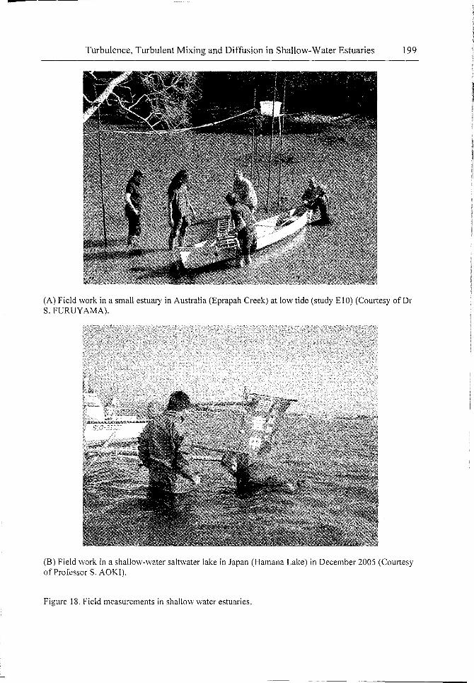
(A) Field work in a small estuary in Australia (Eprapah Creek) at low tide (study EIO) (Courtesy of DrS. FURUYAMA).

(B) Field work in a shallow-water saltwater lake in Japan (Hamana Lake) in December 2005 (Courtesyof Professor S. AOKI).

Figure 18. Field measurements in shallow water estuaries.


5. CONCLUSION

In small estuaries, the predictions of scalar dispersion can rarely be estimated accuratelybecause of a lack of fundamental understanding of the turbulence structure. Detailed turbulentvelocity and suspended sediment concentration measurements were performedsimultaneously and continuously at high frequency for between 25 and 50 hours perinvestigation in shallow-water estuaries with semi-diurnal tides in Australia and Japan (Fig.18). The detailed analyses provided a unique characterisation of the turbulent mixingprocesses and suspended sediment fluxes.

Continuous turbulent velocity sampling at high frequency allowed a detailedcharacterisation of the turbulence field in estuarine systems and its variations during the tidalcycle. The turbulence was neither homogeneous nor isotropic. It was not a purely Gaussianprocess, and the small departures from Gaussian probability distribution were an importantfeature of the turbulent processes. A striking feature of the present data sets was the large andrapid fluctuations in all turbulence characteristics and of the suspended sediment fluxesduring the tidal cycles. This was rarely documented, but an important characteristic of thenewer data sets is the continuous high frequency sampling over relatively long periods. Thefindings showed that the turbulent properties, and integral time and length scales should notbe assumed constant in a shallow estuary. The integral time scales for turbulence andsuspended sediment concentration were similar during flood tides, but differed significantlyduring ebb tides. It is believed that the present results provided a picture general enough to beused, as a first approximation, to characterise the flow field in similar shallow-water estuarieswith semi-diurnal tides. It showed in particular a different response from that observed inlarger, deep-water estuaries.

A turbulent flux event analysis was performed for a 50 hour long field study. The resultsshowed that the large majority of turbulent events had a duration between 0.04 sand 0.3 s,and there were on average 1 to 4 turbulent events per second. A number of turbulent burstingevents consisted of consecutive sub-events, with between I and 3 sub-events per event onaverage for all turbulent fluxes. A comparison with atmospheric boundary layer resultsillustrated a number of similarities between the two types of turbulent flows. Both studiesimplied that the amplitude of an event and its duration were nearly independent.

Overall the present research highlighted some turbulent processes that were rarelydocumented in previous studies. However, an important feature of the present analysis wasthe continuous high frequency sampling data sets collected during relatively long periods, aswell as the simultaneous sampling of both turbulent velocities and suspended sedimentconcentrations.

ACKNOWLEDGMENTS

The writers acknowledge the assistance of and inputs from Prof. Shin-ichi AOKI(Toyohashi University of Technology), Or Richard BROWN (Q.U.T.), John FERRIS(Queensland E.P.A.), and Or Ian RAMSAY (Queensland E.P.A.). They acknowledge furtherthe contribution of the numerous people involved in the field works.

-


REFERENCES

[1] Bauer B.O., Yi, J., Namikas, S.L, and Sherman, DJ. (1998). "Event Detection andConditional Averaging in Unsteady Aeolian Systems." Jl of Arid Env., Vo!. 39, pp.345-375.

[2] Bowden, K.F., and Ferguson, S.R. (1980). "Variations with Height of the Turbulence ina Tidally-Induced Botom Boundary Layer." Marine Turbulence, J.CJ. NIHOUL, Ed.,Elsevier, Amsterdam, The Netherlands, pp. 259-286.

[3] Bowden, K.F. and Howe, M.R. (1963). "Observations of turbulence in a tidal current."Journal ofFluid Mechanics, Vo!. 17, No. 2, pp. 271-284.

[4] Bradshaw, P. (1971). "An Introduction to Turbulence and its Measurement." PergamonPress, Oxford, UK, The Commonwealth and International Library of Science andtechnology Engineering and Liberal Studies". Thermodynamics and Fluid MechanicsDivision, 218 pages.

[5] Chanson, H. (2003). "A Hydraulic, Environmental and Ecological Assessment of aSub-tropical Stream in Eastern Australia: Eprapah Creek, Victoria Point QLD on 4April 2003." Report No. CH52103, Dept. of Civil Engineering, The University ofQueensland, Brisbane, Australia, June, 189 pages.

[6] Chanson, H. (2004). "Environmental Hydraulics of Open Channel Flows." ElsevierButterworth-Heinemann, Oxford, UK, 483 pages.

[7] Chanson, H., Brown, R., Ferris, 1., Ramsay, 1., and Warburton, K. (2005). "PreliminaryMeasurements of Turbulence and Environmental Parameters in a Sub-Tropical Estuaryof Eastern Australia." Environmental Fluid Mechanics, Vo!. 5, No. 6, pp. 553-575(DOl: 10.1007Is 10652-005-0928-y).

[8] Chanson, H., Takeuchi, M., and Trevethan, M. (2008a). "Using Turbidity and AcousticBackscatter Intensity as Surrogate Measures of Suspended Sediment Concentration in aSmall Sub-Tropical Estuary." Journal of Environmental Management, Vo!. 88, No. 4,Sept., pp. 1406-1416 (DOl: 10.10 16/j.jenvman.2007.07.009).

[9] Chanson, H., Trevethan, M., and Aoki, S. (2008b). "Acoustic Doppler Velocimetry(ADV) in Small Estuary : Field Experience and Signal Post-Processing." FlowMeasurement and Instrumentation, Vo!. 19, No. 5, pp. 307-313 (DOl:10.1016/j.f1owmeasinst.2008.03.003).

[10] Digby, MJ., Saenger, P., Whelan, M.B., Mcconchie, D., Eyre, B., Holmes, N., Bucher,D. (1999). "A Physical Classification of Australian Estuaries." Report No. 9,LWRRDC, Australia, National River Health Program, Urban sUb-program, OccasionalPaper, 16/99.

[11] Dyer, K.R. (1997). "Estuaries. A Physical Introduction." John Wiley, New York, USA,2nd edition, 195 pages.

[12] Finnigan, 1. (2000). "Turbulence in Plant Canopies." Ann. Rev. Fluid Mech., Vo!. 32,pp. 519-571.

[13] Fransson, 1.H.M., Matsubara, M., and Alfredsson, P.H. (2005)." Transition Induced byFree-stream Turbulence." Jl ofFluid Mech., Vo!. 527, pp. 1-25.

[14] Fugate, D.C., and Friedrichs, C.T. (2002). "Determining Concentration and FallVelocity of Estuarine Particle Populations using ADV, OBS and LISST." ContinentalShelfResearch, Vo!. 22, pp. 1867-1886.


(I5] Hallback, M., Groth, 1., and Johansson, A.V. (1989). "A Reynolds Stress Closure forthe Dissipation in Anisotropic Turbulent Flows." Proc. 7th Symp. Turbulent ShearFlows, Stanford University, USA, Vol. 2, pp. 17.2.1-17.2.6.

[16] Ham, R. van der, Fromtijn, H.L., Kranenburg, C., and Winterwerp, J.C. (2001)."Turbulent Exchange of Fine Sediments in a Tidal Channel in the Ems/DoIIard Estuary.Part I: Turbulence Measurements." Continental ShelfResearch, Vol. 21, pp. 1605-1628.

[17] Hinterberger, C., Fr6hlich, J., and Rodi, W. (2008). "20 and 3D Turbulent Fluctuations

in Open Channel Flow with Ret = 590 studied by Large Eddy Simulation." FlowTurbulence Combustion, Vol. 80, No. 2, pp. 225-253 (001: 1O.1007/sI0494-007-91222).

[18] Hinze, J.O. (1975). "Turbulence." McGraw-Hill Pub!., 2nd Edition, New York, USA.[19] Hossain, S., Eyre, B., and Mcconchie, D. (2001). "Suspended Sediment Transport

Dynamics in the Subtropical Micro-tidal Richmond Rive... Estuary, Australia."Estuarine, Coastal and ShelfScience, Vol. 52, pp. 529-54 I.

[20] Johansson, A.V., and Alfredsson, P.H. (1982). "On the Structure of Turbulent ChannelFlow." Jl ofFluid Mech., VoI. 122, pp. 295-314.

[2 IJ Kawanisi, K., and Yokosi, S. (1994). "Mean and Turbulence Characteristics in a TidalRiver." Continental ShelfResearch, Vol. 17, No. 8, pp. 859-875.

[22J Kawanisi, K., Tsutsui, T., Nakamura, S., and Nishimaki, H. (2006). "Influence of TidalRange and River Discharge on Transport of Suspended Sediment in the Ohta Floodway." Jl ofHydroscience and Hyd. Eng., JSCE, Vol. 24, No. I, May, pp. 1-9.

[23J Kline, S.1., Reynolds, W.C., Schraub, F.A. and Runstaller, P.W. (l967)."The structureof turbulent boundary layers." Journal of Fluid Mechanics, VOI. 30, No. 4, pp. 741-773.

[24] Koch, C., and Chanson, H. (2005). "An Experimental Study of Tidal Bores and PositiveSurges: Hydrodynamics and Turbulence of the Bore Front." Report No. CH56/05, Dept.of Civil Engineering, The University of Queensland, Brisbane, Australia, July, 170pages.

[25] Larcombes, P. and Ridd, P.V. (1992). "Dry Season Hydrodynamics and SedimentTransport in a Mangrove Creek." Proceedings 6th International Biennial Conf onPhysics ofEstuaries and Coastal Seas, Margaret River WA, Australia, Paper 23. (AlsoMixing in Estuaries and Coastal Seas, Coastal and Estuarine Studies Vol. 50, AGU,New York, USA, 1996, pp. 388-404.)

[26] Montes, J.S. (1998). "Hydraulics of Open Channel Flow." ASCE Press, New-York,USA, 697 pages.

[27J Narasimha, R., Kumar, S.R., Prabhu, A., and Kailas, S.V. (2007). "Turbulent FluxEvents in a Nearly Neutral Atmospheric Boundary Layer." Phi!. Trans. Royal Soc.,Series A, Vol. 365, pp. 841-858.

[28J Nezu, I. (2005). "Open-Channel Flow Turbulence and its Research prospect in the 21stCentury." Jl ofHyd. Engrg., ASCE, Vol. 13 I, No. 4, pp. 229-246.

[29] Nezu, L, and Nakagawa, H. (1993). "Turbulence in Open-Channel Flows." IAHRMonograph, IAHR Fluid Mechanics Section, Balkema Pub/., Rotterdam, TheNetherlands, 281 pages.

[30J Niederschulte, M.A. (1989). "Turbulent Flow Through a Rectangular Channel." Ph.D.thesis, Dept. of Chem. Eng., University of Illinois, Urbana-Champaign, USA, 4 I7pages.

-

[31 ]

[32]

[33]

[34]

[35]

[36]

[37]

[38]

[39]

[40]

[41 ]

[42]

[43]

[44]

[45]

[46]

[47]


Nielsen, P. (1992). "Coastal Bottom Boundary Layers and Sediment Transport."Advanced Series on Ocean Eng., Vo!. 4, World Scientific Pub!., Singapore.Nikora, V., Goring, D., and Ross, A. (2002). "The Structure and Dynamics of the ThinNear-Bed Layer in a Complex Marine Environment: A Case Study in Beatrix Bay, NewZealand." Estuarine, Coastal and ShelfScience, Vo!. 54, pp. 915-926.Osonphasop, C. (1983). "The Measurements of Turbulence in Tidal Currents." PhD.thesis, Dept of Mech. Eng., Monash Univ., Australia.Osterlund, J.M., Lindgren, B., and Johansson, A.V. (2003). "Flow Structures in ZeroPressure-Gradient Turbulent Boundary Layers at High Reynolds Numbers." Eur. JlMechanics B. Fluids, Vo!. 22, pp. 379-390 (DOl: 10. 10 16/S0997-7546(03)00034-7).Piquet, J. (1999). "Turbulent Flows. Models and Physics." Springer, Berlin, Germany,761 pages.Rao, K.N., Narasimha, R., and Narayanan, A.A.B. (1971). "The "Bursting" Phenomenain a Turbulent Boundary Layer." JI ofFluid Mech, Vo!. 48, Part 2, pp. 339-352.Reynolds, O. (1883). "An Experimental Investigation of the Circumstances whichDetermine whether the Motion of Water shall be Direct or Sinuous, and the Laws ofResistance in Parallel Channels." Phi!. Trans. Roy. Soc. Lond., Vo!. 174, pp. 935-982.Reynolds, O. (1887) "On Certain Laws Relating to the Regime of Rivers and Estuaries,and on the Possibility of Experiments on a Small Scale." British Association Report,UK.Rudra Kumar, S., Ameenulla, S., and Prabhu, A. (1995). "MONTBLEX TowerObservations: Instrumentation, Data Acquisition and Data Quality." Proc. Indian Acad.Science (Earth Planet Science), Vo!. 104, No. 2, pp. 221-248.Savenije, H.H.G. (2005). "Salinity and Tides in Alluvial Estuaries." Elsevier,Amsterdam, The Netherlands, 194 pages.Schlichting, H. (1979). "Boundary Layer Theory." McGraw-Hill, New York, USA, 7thedition.Shiono, K., and West, J.R. (1987). "Turbulent Perturbations of Velocity in the ConwyEstuary." Estuarine, Coastal and ShelfScience, Vo!. 25, pp. 533-553.Tachie, M.F. (2001). "Open Channel Turbulent Boundary Layers and wall Jets onRough Surfaces." PhD. thesis, Dept. of Mech. Eng., Univers. of Saskatchewan,Canada, 238 pages.Thorne, P.D., Vincent, C.E., Hardcastle, PJ., Rehrnan, S., and Pearson, N. (1991)."Measuring Suspended Sediment Concentrations using Backscatter Devices." MarineGeology, Vo!. 98, pp. 7-16.Trevethan, M. (2008). "A Fundamental Study of Turbulence and Turbulent Mixing in aSmall Subtropical Estuary." PhD. thesis, Div. of Civil Engineering, The University ofQueensland, 342 pages.Trevethan, M., Chanson, H., and Takeuchi, M. (2007a). "Continuous High-FrequencyTurbulence and Sediment Concentration Measurements in an Upper Estuary."Estuarine Coastal and Shelf Science, Vo!. 73, No. 1-2, pp. 341-350(DOl: 10.10 16/j.ecss.2007.01.0 14).Trevethan, M., Chanson, H., and Brown, RJ. (2007b). "Turbulence and Turbulent FluxEvents in a Small Subtropical Estuary." Report No. CH65107, Hydraulic Model Reportseries, Div. of Civil Engineering, The University of Queensland, Brisbane, Australia,November, 67 pages.


[48] Trevethan, M., Chanson, H., and Brown, R. (2008). "Turbulence Characteristics of aSmall Subtropical Estuary during and after some Moderate Rainfall." Estuarine Coastaland ShelfScience, Vol. 79, No. 4, pp. 661-670 (DOl: 10. 10 16/j.ecss.2008.06.006).

[49] Voulgaris, G., and Meyers, S.T. (2004). "Temporal Variability of Hydrodynamics,Sediment Concentration and Sediment Settling in a Tidal Creek." Continental ShelfResearch, Vol. 24, pp. 1659-1683.

[50] West, J.R. and Oduyemi, K.O.K. (1989). "Turbulence measurements of suspendedsolids concentration in estuaries." Journal ofHydraulic Engineering, ASCE, Vol. 115,No. 4, pp. 457-473.

[51] Xie, Q. (1998). "Turbulent Flows in Non-Uniform Open Channels: ExperimentalMeasurements and Numerical Modelling." Ph.D. thesis, Dept. of Civil Eng., UniversityOf Queensland, Australia, 339 pages.

INTERNET REFERENCES

A Hydraulic, Environmental and {http://www.uq.edu.au/~e2hchans/eprapa.html}Ecological Assessment of a Sub-tropical Stream in Eastern Australia:Eprapah Creek, Victoria Point QLD on4 April 2003Queensland EPA water quality {http://www.epa.qld.gov.au/environmental_managemonitoring ment/water/water quality monitoring/}Eprapah Creek Catchment Landcare {http://eprapah.scouting.net.au/index/projects/landcAssociation Inc. (ECCLA) are.htm}Research publications in hydraulic {http://espace.library.uq.edu.au/listlauthor_ id/193/}engineering and applied fluidmechanics

OPEN ACCESS REPOSITORIES

Reviewed by Professor Michele MOSSA, Politecnico di Bari (Italy)

turbulence, turbulent mixingand diffusion in...

Documents