the effects of cbl on graphical interpretation of ... · the effects of calculator based...
TRANSCRIPT
THE EFFECTS OF CALCULATOR BASED LABORATORIES (CBL) ON GRAPHICAL INTERPRETATION OF KINEMATIC CONCEPTS IN PHYSICS
AT METU TEACHER CANDIDATES
A THESIS SUBMITTED TO THE GRADUATE SCHOOL OF NATURAL AND APPLIED SCIENCES OF
MIDDLE EAST TECHNICAL UNIVERSITY
BY
AHMET FATİH ERSOY
IN PARTIAL FULFILLMENT OF THE REQIREMENTS FOR THE DEGREE OF MASTER OF SCIENCE
IN SECONDARY SCIENCE AND MATHEMATICS EDUCATION
APRIL 2004

Approval of the Graduate School of Natural and Applied Sciences.
____________________________
Prof. Dr. Canan ÖZGEN
Director
I certify that this thesis satisfies all the requirements as a thesis for the degree of
Master of Science.
____________________________
Prof. Dr. Ömer GEBAN
Head of Department
This is to certify that we have read this thesis and that in our opinion it is fully
adequate, in scope and quality, as a thesis for the degree of Master of Science.
____________________________
Dr. Mehmet SANCAR
Supervisor
Examining Committee Members
Assist. Prof Dr. Ceren TEKKAYA ____________________________
Assist. Prof Dr. Jale ÇAKIROĞLU ____________________________
Dr. Ahmet İlhan ŞEN ____________________________
Dr. Mehmet SANCAR ____________________________
Dr. Turgut FAKIOĞLU ____________________________

I hereby declare that all information in this document has been obtained and presented in accordance with academic rules and ethical conduct. I also declare that, as required by these rules and conduct, I have fully cited and referenced all material and results that are not original to this work. Name, Last name: Ahmet Fatih, Ersoy
Signature :

ABSTRACT
THE EFFECTS OF CALCULATOR BASED LABORATORIES (CBL) ON
GRAPHICAL INTERPRETATION OF KINEMATIC CONCEPTS IN PHYSICS
AT METU TEACHER CANDIDATES
Ersoy, Ahmet Fatih
M. S., Department of Secondary Science and Mathematics Education
Supervisor: Dr. Mehmet Sancar
April 2004, 111 pages
Science education should teach students to critically evaluate new
information. Students have difficulties making connections among graphs of
variables, physical concepts and the real world and often perceive graphs as a
picture. Calculator Based Laboratories (CBL) provide immediately available
calculator drawn graphics of objects in motion. Up to date effectiveness of
microcomputers are evaluated but there are few studies on the use of CBL, which are
feasible, easy to use, portable and cheap with respect to microcomputers.
In this study we want to find out the effectiveness of CBL method on the
graphical interpretation of kinematical concepts in physics at METU teacher
candidates. Data will be analyzed with SPSS for Windows program.
The study carried out 2002 – 2003 Spring Semester at Education Faculty in
METU. 32 students from two classes were involved in the study. All students
administered TUG-K (Test of Understanding Graphs – Kinematics) before and after
iv

the CBL activities.
The data obtained from the administration of the pretests and the posttest
were analyzed statistical technique of Paired Samples T Test. The statistical analysis
failed to show any significant difference in the students’ understandings of
kinematics graphs.
Keywords: Physics Education, Micro-Computer Based Laboratories,
Calculator Based Laboratories.
v

ÖZ
HESAP MAKİNESİ DESTEKLİ FİZİK EĞİTİMİNİN ODTU ÖĞRETMEN
ADAYLARININ KİNEMATİK KAVRAMLARININ GRAFİKSEL
YORUMLAMALARI ÜZERİNE ETKİSİ
Ersoy, Ahmet Fatih
Yüksek Lisans, Orta Öğretim Fen ve Matematik Alanları Eğitimi Bölümü
Tez Yöneticisi: Dr. Mehmet Sancar
Nisan 2004, 111 sayfa
Fen eğitimi öğrencilere yeni bilgileri eleştirel gözle değerlendirebilmeyi
öğretmelidir. Öğrenciler grafik değişkeleri ile fiziksel kavramları ve gerçek dünyayı
ilişkilendirmede sorun yaşamakta ve genellikle grafikleri birer resim olarak
algılamaktadırlar. Günümüze kadar bilgisayar destekli laboratuarlar üzerine bir çok
araştırmalar yapılmış fakat HeMa Lab üzerine yeterince çalışma yapılmamıştır.Hesap
Makineleri Destekli Laboratuarlar (HeMa Lab) hareketli nesnelerin grafiklerini
anında verebilmektedirler. HeMa Lab aynı zamanda bilgisayar destekli laboratuarlara
göre fiyat olarak uygun, kullanımı kolay ve taşınabilirdirler.
Bu çalışmada biz HeMa Labın ODTÜ öğretmen adaylarının fizikteki
kinematik kavramlarının ve grafiklerinin kavranmasındaki etkinliğini bulmaya
çalıştık. Bilgiler Windows için SPSS programı ile analiz edilecektir.
Çalışma 2002 – 2003 bahar döneminde ODTÜ Eğitim Fakültesinde
yapılmıştır. 2 sınıftan 32 öğrenci çalışmaya katılmıştır. Bütün öğrenciler HeMa Lab
vi

aktivitelerinden önce ve sonra TUG – K (Kinematik Grafiklerini Anlama Testi)
Testini ön ve son – test olarak almışlardır.
Elde edilen bulgular T – Testi ile analiz edilmiştir. Test sonuçları
öğrencilerin kinematik grafiklerini anlamadaki başarı değişikliklerini istatistiksel
olarak gösterememiştir.
Anahtar Kelimeler: Fizik Eğitimi, Bilgisayar Destekli Laboratuarlar, Hesap
Makineleri Destekli laboratuarlar (HeMa Lab).
vii

To my wife Tuğba and
To my daughter Rana
viii
ACKNOWLEDGEMENTS
This is perhaps the easiest and hardest chapter that I have to write. It will be simple to
name all the people that helped to get this done, but it will be tough to thank them enough. I
will nonetheless try…
It is a pleasure to thank the many people who made this thesis possible. It is difficult
to overstate my gratitude to my supervisor, Dr. Mehmet Sancar. With his enthusiasm, his
inspiration, and his great efforts to explain things clearly and simply, he helped to make this
work fun for me. Throughout my thesis-writing period, he provided encouragement, sound
advice, good teaching, good company, and lots of good ideas. I would have been lost without
him. I am grateful to Prof. Dr. Yaşar Ersoy, Assist. Prof. Dr. Ali Eryilmaz, Assist. Prof. Dr.
Ceren Tekkaya, Assist. Prof. Dr. Jale Çakıroğlu for guiding me through the writing of the
thesis, and for all the corrections and revisions made to text that is about to be read. It became a
lighter and more concise thesis after their suggested improvements.
I am indebted to my many student colleagues for providing a stimulating and fun
environment in which to learn and grow. I am especially grateful to Almer Abak, Özlem
Hardal, Gülcan Çetin, Eren Ceylan, Abdullah Topçu, and Murat Ulubay.
My final words go to my family. In this type of work the relatives are always
mistreated. I must therefore thank my wife Tuğba for putting up with my late hours, my
spoiled weekends, my bad temper, but above all for putting up with me and surviving the
ordeal. With all the ‘cells’ passing in this world it is a fortune that ours ‘collided’. I wish to
thank my parents, Arif and Leylâ Ersoy. They bore me, raised me, supported me, taught me,
and loved me. And also I am grateful for other members of my family Sümeyra and Ekrem
Yüce and my nephews Zeynep Beyza and Ahmet Yüce.
ix
TABLE OF CONTENTS
ABSTRACT................................................................................................................iv
ÖZ…… .......................................................................................................................vi
ACKNOWLEDGEMENTS ........................................................................................ix
TABLE OF CONTENTS.............................................................................................x
LIST OF TABLES ....................................................................................................xiii
LIST OF FIGURES ..................................................................................................xiv
LIST OF SYMBOLS .................................................................................................xv
CHAPTERS .................................................................................................................1
1. INTRODUCTION ................................................................................................... 1 1.1. The Main Problem .......................................................................................5 1.1.1 The Sub – Problem: ............................................................................5 1.2. Hypothesis ...................................................................................................5 1.3. Definition of Important Terms.....................................................................6 1.4. Significance of the Study.............................................................................7
2. REVIEW OF RELATED LITERATURE............................................................... 9 2.1. Laboratory in Science Teaching ..................................................................9 2.2. Graphs and Graphing Ability.....................................................................10 2.2.1. Difficulties in Kinematics Graphing Skills.....................................12 2.3. Studies on Microcomputer and Calculator Based Laboratories ...............14 2.4. Benefits of Calculator Based Laboratories ...............................................18 2.5. Summary of the Literature Review...........................................................22 3. METHODS ............................................................................................................ 27 3.1. Population and Sample .............................................................................27
x

3.2. Variables ...................................................................................................28 3.2.1. Dependent Variables.......................................................................28 3.2.2. Independent Variables ....................................................................29 3.3. Measuring Tools ........................................................................................29 3.3.1. Test of Understanding Graphs Kinematics (TUG-K).....................29 3.3.2. Activity Sheets................................................................................31 3.3.3. Questionnaire: Teacher Candidates’ Opinions about the Treatment.......................................................................................31 3.3.4. Calculator Attitude Test.................................................................32 3.2.5. Physics Attitude Test .....................................................................32 3.3.6. Validity and Reliability of the Measuring Tool ............................32 3.4. Teaching and Learning Materials ..............................................................34 3.5. Procedure ...................................................................................................37 3.6. Analysis of Data.........................................................................................38 3.6.1. Descriptive and Inferential Statistics.............................................39 3.6.2. Analysis of Teacher Candidates’ Opinions about the Treatment ..39 3.7. Assumptions and Limitations ....................................................................39
4. RESULTS .............................................................................................................. 41 4.1. Descriptive Statistics..................................................................................41 4.2. Inferential Statistics ...................................................................................43 4.2.1 Missing Data Analysis...................................................................44 4.2.2 Assumptions of Paired-Samples T Test.........................................44 4.2.3 Paired-Samples T Test...................................................................45 4.2.4 Assumptions of Wilcoxon Signed Ranks Test ..............................45 4.2.5 Wilcoxon Signed Ranks Test ........................................................46
xi
4.2.4 Null Hypothesis .............................................................................46 4.3 Results of the Questionnaire: The Teacher Candidates’ Opinions About The Treatment. ...........................................................................................46 4.4 Summary of the Results .............................................................................49
5 CONCLUSIONS, DISCUSSION AND IMPLICATION ...................................... 52 5.1. Conclusions................................................................................................52 5.2. Discussion of the Results ...........................................................................53 5.3. Internal Validity .........................................................................................54 5.4. External Validity........................................................................................56 5.5. Implications ...............................................................................................57 5.6. Recommendations for Further Research....................................................59
REFERENCES .......................................................................................................... 60
APPENDICES ........................................................................................................... 69 A. Objective List.................................................................................................69 B. Test of Understanding of Graphs – Kinematics ............................................70 C. CBL Activities ...............................................................................................82 Acticitiy 1 – Graphics Matching ..............................................................82 Acticitiy 2 – Toy Car (Constant Velocity) ................................................87 Acticitiy 3 – Toy Car (Constant Acceleration I) .......................................92 Acticitiy 4 – Toy Car (Constant Acceleration II) ......................................97 D. Objective Activity Table..............................................................................102 E. Physics Attitude Test....................................................................................103 F. Calculator Attitude Test................................................................................105 H. Questionnaire: Teacher Candidates’ Opinions about the Treatment ...........106 F. Raw Data ......................................................................................................107
xii

LIST OF TABLES
TABLE
3.1 Characteristics of the Sample ..............................................................................28
3.2 Identification of Variables...................................................................................30
3.3. Point Biserial Coefficients and Number of Students Selecting a Particular
Choice for Each Test Item for PRETEST...........................................................35
3.4. Point Biserial Coefficients and Number of Students Selecting a Particular
Choice for Each Test Item for POSTTEST ........................................................36
3.5. Descriptive Statistics About the TUG – K Test ..................................................34
4.1 Descriptive Statistics of Students’ TUG-K Scores (N = 32) ...............................42
4.2 Descriptive Statistics of Students’ AGE, CGPA, and PHYS111 ........................44
4.3 Paired-Samples T Test (N = 32) ..........................................................................45
4.4 Students’ Responses To Open – Ended Questions (N = 22)................................47
4.5 Paired-Samples T Test of the TUG – K Objectives (N = 32) ..............................45
4.6 Partial Correlations among the IVs of the Study .................................................51
xiii

LIST OF FIGURES
FIGURES 4.1 Histograms with Normal Curves Related to the TUG-K PRETEST and
POSTTEST Scores (N = 32)...............................................................................43
xiv

LIST OF SYMBOLS
SYMBOLS
ACTSCORE : Students’ Scores of CBL Activities
POSTTEST : Students’ Scores of TUG – K as Posttest
SCOREDIF : Students’ Difference Scores between POSTTEST and PRETEST
PRETEST : Students’ Scores of TUG – K as Pretest
PHYS111 : Students’ Physics 111 Course Grades
PHYSAT : Students’ Scores of Physics Attitude Test
REASON : Students’ Reason of Choosing Their Departments
CALAT : Students’ Scores of Calculator Attitude Test
CGPA : Students’ Cumulative Grade Point Averages
LGPA : Students’ Grade Point Averages of the Previous Semester
FGPA : Students’ Grade Point Averages When They Had Taken Physics 111
MED : Education Level of Students’ Mothers
FED : Education Level of Students’ Fathers
CBL : Calculator Based Laboratories
CBR : Calculator Based Ranger
NC : Number of Childs in Students’ Family
DV : Dependent Variables
IV : Independent Variables
N : Sample Size
xv

1
CHAPTER 1
INTRODUCTION
Science education should teach students to critically evaluate new
information. This is especially true given the well documented exploration of
information. Experts estimate that scientific information doubles every year. As we
entered so called “information age” we need to prepare students to assess new things
effectively (Nachmias, & Linn, 1987).
Science education contributes to the growth and development of all
students, as individuals, as responsible and informed members of society. Science
education aims helping students to develop knowledge and a coherent understanding
of the living, physical, material, and technological components of their environment,
encouraging students to develop skills for investigating the living, physical, material,
and technological components of their environment in scientific ways, promoting
science as an activity that is carried out by all people as part of their everyday life
(The On – Line Teaching Center).
Similarly physics education has similar aims. The most important ones are
to find ways to help students learn physics more effectively and efficiently, to
understand concepts more deeply (Meltzer, 2003). This may be done with a proper
curriculum. There should be connections in the curriculum to everyday life so that
the students are trained in the art of finding a physical explanation for what they

2
experience. There should be opportunities to experience the scientific method so that
the students can apply it when making critical investigations. The physics education
should make a contribution to the development of the student’s view of the world,
develop scientific literacy, experimental skills, and communication skills and train
the student in problem solving with mathematical methods (Olme, 2000).
One of the firs topics taught in a traditional high-school physics course is
motion, including the concepts of position, velocity and acceleration. Graph of
objects in motion are frequently used since they offer a valuable and alternative to
verbal and algebraic descriptions of motion by offering students another way of
manipulating the developing concepts (Arons, 1990). Graphs are the best summary
of functional relationship. Many teachers consider the use of graphs in a laboratory
setting to be critical importance for reinforcing graphing skills and developing an
understanding of many topics in physics, especially in motion (Svec, 1999).
If graphs are to be valuable tool for students then we must know the
students level of graphing ability. Studies have identified difficulties with such
graphic abilities. Students have difficulties making connections among graphs of
different variables, physical concepts, and the real world, and they often perceive
graphs as just a picture (Linn, Layman & Nachmias, 1987).
From the time when the first calculator invented electronic calculator
evolved from a machine that could only carry out simple four – function operations
into one that can perform highly technical algebraic and symbolic manipulations
instantly and accurately. Calculators are valuable educational tools that allow

3
students to reach a higher level of mathematical power and understanding by
reducing time that was spent on learning and performing paper and pencil work.
Using calculators allow students and teachers to spend more time on developing
understanding of concepts, reasoning and applications. In the past paper and pencil
were only tools available but now calculators are available and they are better tools
to do most of the computations and manipulations that were done with paper and
pencil. Appropriate use of technology and associated pedagogy will get more
students to develop useful understanding skills (Pomerantz, 1997).
Calculator Based Laboratory™ (CBL) and Calculator-Based Ranger™
(CBR), which is a data collection device designed to collect and analyze real-world
motion data, such as distance, velocity and acceleration, devices are designed to
collect data via various probes and then store or feed the data into a computer or
calculator. This data can then be analyzed and displayed using many different
representations, enabling the student to gather the data and then graph it either at a
later time or simultaneously. It seems to be the consensus that the study of graphs
can lead to a deeper understanding of physical concepts. However, there are many
problems that students have with regard to graphing and modeling (Douglas, 1999).
Laboratory activities which focus on graphing more than traditional labs are
valuable in the investigation of students’ use of graphs. CBL provide immediately
available, calculator drawn graphics of objects in motion. CBL is centered around a
sonic ranger, which measures the distance to an object and creates a position versus
time graph of the objects motion in real time. Learners can move and see the graph

4
of their motion on the calculator display respond to their motion. The CBL provide
an excellent to explore the connection between graphing skills and understanding of
motion concepts. Students can connect with concrete, kinesthetic experiences. The
ability of calculators to display data graphically is cited as one of the reasons why
CBL is effective.
Finally ,with a couple of words, with the CBL the world becomes your
laboratory allowing students to collect data anywhere, it is portable and does not
need an electrical supply, students learn the reason for graphs and how to interpret
them, more time is spent on developing concepts, less time collecting data, during
the data analysis there is chance for discussion enabling teachers to gauge the
understanding levels of students, activities can be repeated easily with multiple
variables, technology can be used successfully with a wide variety of students,
students learn to problem solve, data can be collected for various periods of time,
multiple probes can be used with the same interface.
In the light of these findings the MBL and CBL studies and its implications
are used in most of the developed countries. In Turkey there are only a few
researches done on MBL and there is none in CBL usage in physics laboratories. It is
important to do similar researches in our country in order to use and develop the
CBL activities.
The general purpose of this study is to find out the effectiveness of CBL on
understanding and interpreting kinematics graphs.

5
1.1. The Main Problem
What is the effect of Calculator Based Laboratories (CBL) on students’
understandings of kinematics graphs?
1.1.1 The Sub – Problem:
The sub – problems (SP) are:
SP1: Is there a significant effect of CBL on students’ understandings of
kinematics graphs?
SP2: What are the opinions of the teacher candidates about the treatment
and its results?
1.2. Hypothesis
The problem stated above was tested with the following hypothesis that is
stated in null form.
Null Hypothesis
H0: µ2 - µ1 = 0
2: Scores on TUG-K (test of understanding graphs-kinematics) as posttest, 1: Scores
on TUG-K (test of understanding graphs-kinematics) as pretest.

6
There will be no significant effect of CBL on students’ means of
POSTTEST and PRETEST scores.
1.3. Definition of Important Terms
CBL: Calculator based laboratories where calculators are used to collect
data and display them graphically.
CBR: The CBR is a data collection device. Designed for teachers who want
their students to collect and analyze real-world motion data, such as distance,
velocity and acceleration.
Motion Detector: Motion Detector is a sonic device to collect real-world
motion data, such as distance, velocity and acceleration.
Kinematics Graphics: Kinematics graphics are position versus time, velocity
versus time, and acceleration versus time graphics.
TUG-K: TUG-K is Test of Understanding Graphs-Kinematics. The test is
developed to testing student interpretation of kinematics graphs (Beichner, 1994).
AGE: The age of students in years, participated in the study. This
information was taken form the university registration office.
GENDER: It is the fact of being male or female. This information was
collected at the time of pretesting.
PRETEST: Students’ achievement scores from the TUG – K as a pretest.

7
POSTTEST: Students’ achievement scores from the TUG – K as a posttest.
SCOREDIF: Students’ score difference between the POSTTEST and
PRETEST scores.
PHYS111: Students’ grade of Introduction to Physics I (Phys111) course.
CGPA: Students’ cumulative grade point averages.
PHYSAT: Students’ physics attitude scores. This information was collected
at the time of pretesting.
CALAT: Students’ calculator attitude scores. This information was
collected at the time of posttesting.
ACTSCORE: Students’ scores taken from the CBL activities.
1.4. Significance of the Study
Up to date use of microcomputers are evaluated but there are a few studies
on the effectiveness of the use of CBL’ s, which are feasible, easy to use, portable
and cheap with respect to computers (The price of three computers are equal to 10
calculators with necessary equipments). And also other problem of labs is to find
enough space to install computers. However there won’t be such problem if we use
calculators.
This study will be the first study on Calculator Based Laboratories and
Physics in Turkey. The study will help other researches who may work on related

8
topics. Graphic calculators are widely used in other education areas such as
mathematics, biology and chemistry. And there are many researches done on this
area. There are several studies on CBL and its usage in mathematics education in
Turkey. This study aims to show graphic calculators can be also used in Physics
Lectures in Turkey.

9
CHAPTER 2
REVIEW OF RELATED LITERATURE
This chapter devoted to the presentation of theoretical and empirical
background for this study.
2.1. Laboratory in Science Teaching
Galileo Galilee established experimentation as a foundation of modern
science through the simple act of dropping two iron balls from the Tower of Pisa.
Though debatable whether he actually performed that experiment, discussion in his
Dialogues Concerning the Two New Sciences shows clearly the power and
importance of experimental observations in convincing others of the correctness of a
particular scientific theory or hypothesis. The history of science from Galilei on has
primarily been the reconciliation of theory with imperfect experimental data
(Forinash & Wisman 2001).
Laboratory teaching is one of the hallmarks of education in the sciences
(Hegarty, 1987; Tobin, 1990). Laboratory work is seen as an integral part of most
science courses and offers an environment different in many ways from that of the
"traditional" classroom setting (Henderson, & Fisher 1998).
Science in the laboratory was intended to provide experience in the
manipulation of instruments and materials, which was also thought to help students
10
in the development of their conceptual understanding. It is hard to imagine learning
to do science, or learning about science in general, without doing laboratory or
fieldwork. Since experimentation underlies all scientific knowledge and
understanding, laboratories are wonderful settings for teaching and learning science
(Trumper, 2002).
2.2. Graphs and Graphing Ability
Fey (as cited in Kwon, 2002) states that there are three mathematical
representations of real – world data: (a) tabular representations, (b) algebraic
representations, and (c) graphic representations. Tabular representations are useful in
showing data with varying parameters. Algebraic representations specify the exact
relationship between variables, but neither give a simple example nor a visual image
(Goldenberg, 1987). Graphical representations, however, provide an image within
the limits of the graph. Graphing representations are frequently used, since they
provide a vulnerable alternative to verbal and algebraic description by offering
students another way of interpreting data and developing concepts (Padilla, 1995).
Graphs provide an invaluable aid in solving arithmetic and algebraic problems and
representing relationships among variables. Graphs display mathematical
relationships that often can not be easily recognized in numerical form (Arkin &
Colton, 1940). Also graphs display trends as geometric patterns that our visual
systems encode easily (Pinker, 1983). Graph construction and interpretation skills
are obviously important for the development of scientifically literate individuals
(Ates & Truman, 2003). McKenzie and Padilla (1986) stated that a graph is an

11
important tool in enabling students to predict relationships between variables and to
make the nature of these relationships concrete. Graphs also provide a powerful tool
for studying complex relationships, and there are useful means of communicating
otherwise difficult to describe information (Norman, 1993).
Kirean (as cited in Kwon, 2002) stated that graphs were rarely taught with
purpose of viewing the whole picture; instead, they were often used as another way
of representing a relationship that was initially depicted in an algebraic
representation in the past. Therefore, most graphical interpretation activities involved
the use of point – wise methods applied to basic functions, such as linear, quadratic,
and trigonometric equations. Also students mainly learned to construct a graph from
a given set of ordered pairs, without reasoning about the physical context in which
the number pairs were introduced, and computing function values.
The ability to comfortably work with graphs is a basic skill of the scientist.
"Line graph construction and interpretation are very important because they are an
integral part of experimentation, the heart of science." A graph depicting a physical
event allows a glimpse of trends which cannot easily be recognized in a table of the
same data. Mokros and Tinker (1987) note that graphs allow scientists to use their
powerful visual pattern recognition facilities to see trends and spot subtle differences
in shape. In fact, it has been argued that there is no other statistical tool as powerful
for facilitating pattern recognition in complex data. Graphs summarize large amounts
of information while still allowing details to be resolved. The ability to use graphs
may be an important step toward expertise in problem solving since "the central

12
difference between expert and novice solvers in a scientific domain is that novice
solvers have much less ability to construct or use scientific representations". Perhaps
the most compelling reason for studying students' ability to interpret kinematics
graphs is their widespread use as a teaching tool.
2.2.1. Difficulties in Kinematics Graphing Skills
McDermott, Rosenquist and Van Zee (1987) studied on difficulty in
connecting graphs to physical concepts and difficulty in connecting graphs to the real
world. McDermott el al. (1987) categorized 10 difficulties students had in the
graphing of kinematics data under two main categories.
1. Difficulties in connecting graphs to physical concepts:
• Discriminating between the slope and the height of a graph.
• Interpreting changes in height and changes in slope.
• Relating one type of graph to another.
• Matching narrative information with relevant features of a
graph.
• Interpreting the area under a graph.
2. Difficulties in connecting graphs to real world:
• Representing a continuous motion with a continuous line.
13
• Separating the shape of a graph from the path of the motion.
• Representing a negative velocity on a velocity versus time
graph.
• Representing a constant acceleration on acceleration versus
time graph.
Some other difficulties were noted (Mokros et al, 1987; Mcdermott, et al.,
1987; Goldberg & Anderson, 1989; Nachmias et al., 1987) that students perceive
graphs as a picture, they confuse slope with the height of the graph and they also
confuse the shape of the graph and the path of the motion.
In addition to above Beichner (1994) studies on the process of developing
and analyzing a test in order to report students’ problems with interpreting
kinematics graphs shown that students also have problems on recognizing the
meaning of areas under the kinematics graphs. Students successfully find the slope of
lines which pass through the origin but they have difficulties in determining the slope
of a line if it does not go through the origin. One another difficulty is distinguishing
between distance, velocity and acceleration (variable confusion). They often believe
that graphs of these variables should be identical and appear to readily switch axis
labels from one variable to another variable without recognizing that the graphed line
should also changed.
14
2.3. Studies on Microcomputer and Calculator Based Laboratories
Physics teachers often report that their students cannot use graphs to
represent physical reality. The types of problems physics students have in this area
have been carefully examined and categorized. Several of these studies have
demonstrated that students entering introductory physics classes understand the basic
construction of graphs, but have difficulty applying those skills to the tasks they
encounter in the physics laboratory (Beichner, 1994).
In recent years there has been a growing belief that technology should
feature in the curriculum of all ages. Pupils should have adequate opportunity to
learn about technology and its interaction with the individual, society and
environment, and to develop the ability to engage in technological tasks through
personal experience (Stewart, 1987). Many pupils have a limited and confused idea
of what technology entails (Rennie, 1987; Rennie & Silletto, 1988). Science teachers
tend to hold a narrow view that technology is the application of science. The
difference between vocational education in the past (which usually was oriented to
low achievers) and today's technology education is not always clear. Steps must be
taken to present technology in an attractive manner that stimulates interest, motivates
students and illustrates various aspects of modem technology (Barak & Eisenberg,
1995).
Svec (1999) studied on the relative effectiveness of traditional lab method
and the microcomputer based laboratories (MBL) for engendering conceptual change
in students and to investigate students’ ability to interpret and use graphs to help

15
them better learn the kinematics concepts and apply this understanding of those
concepts to new non-graphical problems. Subjects were 553 students enrolled in
general physics and physics for elementary teachers’ courses. The results on the
Graphic Interpretation Skills Test and Motion Content Test indicated significant
differences between a traditional laboratory and MBL. MBL was more effective at
engendering conceptual change in students.
Berg and Philips (1994) investigated relationship between logical thinking
structures and the ability to construct and interpret line graphs. Seventy two subjects
in 7th, 9th, and 11th graders were administered individual Piagetian tasks to assess
five specific mental structures: (a) placement and displacement of objects, (b) one-
one multiplication of placement and displacement relations, (c) multiplicative
measurements, (d) multiplicative seriation, and (e) proportional reasoning. The
results of the study shown that students who had not developed the logical thinking
structures in this study were at a severe disadvantage in graphic situations. Mental
structures are needed in order to manipulate some forms of content and graphic
representations. Without cognitive development students are depending upon their
perceptions and low level thinking. Most of the students in elementary grades and
many junior high and secondary schools not have mental structures to understand
line graphs. Therefore, expecting all students to develop an understanding of
graphics is illusory, at least until we facilitate the development of the mental tools
needed to grapple with graphs.

16
Nachmias et al. (1987) studied on the effect of the use of MBL and explicit
instruction on students’ critical evaluation skills. Subjects were 249 eight-graders in
a suburban middle school in California. The Critical Evaluation of Graphs (CEG)
instrument was devised to establish how students evaluated MBL generated
information is assessed five causes to invalid or unreliable graphs: (a) graph scaling,
(b) probe setup, (c) probe calibration, (d) probe sensitivity, (e) experimental
variation. Result of the study showed that students unquestioningly accept computer
presented data; they only linked this information to their other knowledge of natural
world.
Beichner (1990) studied on real time MBL experiments, which allow
students to “see” and at least in kinematics exercises, “feel” the connection between
a physical event and its graphical representation. Graph production was synchronized
with motion reanimation so that students will saw a moving object and its kinematics
graph simultaneously. Subjects were 237 students that are 165 high school and 72
were college students. As a result there were no significant difference between
students assigned to the different groups but there was significant learning overall.
Redish, Saul, Steinberg (1997) studied on the effectiveness of active
engagement of microcomputer based laboratories. Subjects were 470 engineering
students. As a result targeted MBL tutorials can be effective in helping students
building conceptual understanding, but do not provide complete solution to the
problem of building a robust and functional knowledge for many students.

17
Interpreting graphs is widely recognized as being an important goal of
mathematics study. Yet students face many conceptual obstacles in learning to make
sense of position-versus-time graphs. A calculator-based motion lab allows students
to bring these graphs to life by turning their own motion into a graph that can be
analyzed, investigated, and most important, interpreted in terms of how they actually
moved. The investigation of motion can become a rich site for building students'
intuitions about the concept of rate of change and for developing skills in creating
and interpreting graphs. The kinesthetic activity of motion becomes a powerful
means for students to understand position-time graphs. The study of changes in
motion need not be reserved for students in precalculus or calculus classes. (Doerr &
Rieff, 1999).
Dick and Dunham (2000) states that students have trouble with motion
graphs even when they understand the mathematical concepts. Students also have
trouble discriminating between the slope and the height of a graph, relating one type
of graph to another.
Since April, 1996, Kanazawa Technical College has offered a cross-
curricular course for first-year and second-year students using a TI-83 (Graphing
Calculator) and a Computer Based Laboratory (CBL). The goal of the course is for
students to learn about the connection between mathematics and physics through
hands-on activities. Students conduct experiments on the motion of a person
walking, the dropping of an object, the cooling rate of water, the motion of a
swinging pendulum, and sound waves. The following findings were obtained: Most

18
students (a) replaced their naive assumptions regarding the laws of physics with
scientific concepts; (b) independently made connections between the results of
experiments and their previous mathematical knowledge; (c) reported that their level
of interest in physical phenomena and science had either not decreased or had
improved, (d) valued mathematics more, and (e) realized the importance of
cooperative work. The use of CBL and TI-83s changed not only the authors’
teaching style but also students’ attitudes. Students had ownership of their
experiments, and they engaged in higher-order thinking skills such as making
predictions, analyzing data, and modeling data with equations. As a result, students
became more interested in learning mathematics and science (Saeiki et al., 2001).
Middle school students can learn to communicate with graphs in the context
of appropriate Calculator Based Ranger (CBR) activities. The use of CBR activities
developed the three components of students’ graphic abilities which are interpreting,
modeling and transforming significantly. The study indicates that the CBR activities
are pedagogically promising for enhancing graphing ability of physical phenomena
(Kwon, 2002).
2.4. Benefits of Calculator Based Laboratories
When students work with graphing calculators, they have the potential to
work much more intelligently than they could if they were not using this valuable
resource; they form an "intelligent partnership" with the graphing calculator (Jones,
1996). "In almost all cases, students taught with calculators (but tested without

19
technology) had achievement scores for computation as high as or higher than those
taught without technology. With calculators, students had higher problem-solving
scores, better attitudes toward mathematics, and better self-concepts of their own
ability to do mathematics. Recent studies suggest that graphing calculators and
computer symbolic algebra systems can be just as beneficial to student learning"
(Dunham, 1993).
Dunham's review of research (1993) reports that many students who use
graphing technology place at higher levels in hierarchy of graphical understanding;
are better able to relate graphs to their equations; can better read and interpret
graphical information; obtain more information from graphs; have greater overall
achievement on graphing items; are better at "symbolizing", that is, finding an
algebraic representation for a graph; better understand global features of functions;
increase their "example base" for functions by examining a greater variety of
representations; and better understand connections among graphical, numerical, and
algebraic representations Moreover, they: had more flexible approaches to problem
solving; were more willing to engage in problem solving and stayed with it longer;
concentrated on the mathematics of the problem and not on the algebraic
manipulation; solved non-routine problems inaccessible by algebraic techniques; and
believed calculators improved their ability to solve problems' (Dunham & Dick,
1994).
In studies where graphing technology was in use, students were more active,
and they participated in more group work, investigations, problem solving, and
20
explorations. Teachers lectured less and were often used by students as more of a
consultant than a task-setter (Dunham et al., 1994).
"Students who use graphing calculators are better able to read and interpret
graphs, understand global features of graphs, relate graphs to their equations, and
make connections among multiple representations of functions" (Dunham, 1996).
Technology based tools are supporting teachers as they work to change that
trend and revise the way science is taught. Many can remember science lectures,
discussions of data, and chalk-board-etched formulas. Contrast this with the current
generation of students accustomed to video games, computers and other
technologies, and MTV. How can teachers capture the attention of these students and
excite them about math and science? Teachers are being encouraged to make science
more interesting, and technology-based tools are assisting that effort. The Texas
Instruments' Calculator-Based Laboratory System provides students with hand-held
technology that allows them to get actively involved in experimentation. As in real-
world scenarios, they can gather data, inside or outside the classroom; analyze the
data they have found; solve problems and ask questions; and draw conclusions. They
can see how science applies to the world around them by experiencing it firsthand
(Curriculum Administrator, 1997).
Mathematical investigations of motion by middle school students can be
accomplished with a motion lab consisting of a graphing calculator, a Calculator
Based Laboratory (CBL) unit, and a motion detector. Students can run numerous
trials in a short time, since each trial takes only a few seconds and is followed by an

21
immediate visual representation of the motion. We have designed for pre – algebra
students a suitable activity that begins with an exploration of simple distance-versus-
time graphs. This activity is best done over several class periods by small groups of
three or four students, followed by group presentations or whole-class discussion.
Students with limited exposure to graphs rapidly comprehend the visual
representations produced by the motion-detecting system. Since their own motion
produces the graphs, students are quick to experiment and are readily able to
describe the graphs in terms of their own motion. Students begin to describe a graph
in terms of how fast they moved (slope) and where they started (y-intercept) (Doerr
& Rieff, 1999).
The motion detector, the CBL unit, and the graphing calculator create a
flexible and easy-to-use motion lab with which pre – algebra students can investigate
the concepts of rate of change and velocity through the kinesthetic experience of
their own motion. In instructional settings that blend small-group activities with
whole-class discussion, we have found that seventh and eighth graders are eager to
engage in these investigations and discussions. The technology gives students the
opportunity to test their conjectures, to experiment with mathematical ideas, and to
use and develop mathematical language for change and variation. Although we have
shown only one activity, this motion lab can be used with activities that further
quantify the notions of speed, explore periodic motion, and investigate intersecting
linear graphs. Since students themselves are engaged in creating the motion,
interpreting the graphs comes easily (Doerr et al., 1999).

22
The world of science has always fascinated young minds (Welker, 1999).
He used CBL activities in amusement parks and tested students’ learning’s about
motion theories. The students are first asked to hypothesize the acceleration statistics
as they wait to get on the ride. They sketch out graphs such as Position vs. Time,
Height vs. Time and Velocity vs. Time. After they gather these data, students went
back to class and compare their original motion theories to the actual statistics
gathered from the probe. To determine if students truly understand motion theory
after their amusement park experience, the Physics and Math teachers give students a
mythical ride with wild twists and turns. Students are asked to create graphs similar
to the ones made at the park. Welker (1999) states that hands – on science lessons
have never been so fun. Thanks to portable technology, it is possible to bring abstract
theories, such as the effect of motion, to life in a whole new way.
Students have many difficulties interpreting graphs of kinematics variables.
These difficulties are often based on misconceptions. Students cannot repair their
misconceptions until they are confronted by them. Laboratory activities using MBL
or CBL instruments supply a powerful setting and foster the opportunity for student
discourse, both student – student and student – teacher (Dick et al., 2000).
2.5. Summary of the Literature Review
• The most powerful and important way of convincing the correctness of a
particular scientific theory or hypothesis is experimental observations.
• Laboratory teaching is one of the hallmarks (Hegarty, 1987; Tobin, 1990)

23
and an integral part of science education that offers a different
environment from traditional classroom settings (Henderson & Fisher,
1998).
• Science laboratories are intended to provide experience in the
manipulation of instruments and materials which help students to develop
conceptual understanding (Trumper, 2002).
• Graphical representations are the most valuable and useful way of
representing the real world information with regard to tabular and
algebraic representations (Kwon 2002).
• Graphics summarize large amount of data and this makes the graphs most
powerful visual pattern to recognize the complex data and make them an
integral part of experimentation (Makos et al., 1987).
• Science teachers have a narrow view that technology is the application of
science. Technology in science classes may stimulate interest, motivate
students and illustrate various aspects of modern technology (Barak et al.,
1995).
• Svec (1999) showed that microcomputer based laboratories (MBL) was
more effective than traditional laboratories at engendering conceptual
change in students.
24
• Students unquestioningly accept computer presented data; they only
linked this information to their other knowledge of natural world.
• Beichner (1990) stated that MBL experiments have significantly affects
students overall learning.
• MBL tutorials were effective in helping students building conceptual
understanding of students’ but do not provide complete solution to the
problem of building robust and functional knowledge for many students
(Redish et al., 1997).
• A Calculator Based Laboratory (CBL) allows students to bring graphs to
life by turning their own motion into motion in to graph that can be
analyzed, investigated, and most important, interpret in terms of how they
actually moved (Doerr et al., 1999).
• Dick et al. (2000) stated that students have trouble with motion graphs
even they understand the mathematical concepts.
• The use of Calculator Based Laboratories (CBL) made students (a)
replace their naive assumption of scientific concepts; (b) independently
made connections between the results of experiments and their previous
mathematical knowledge; (c) level of interest in physics had improved,
(d) realized the importance of group work (Saeki et al., 2001).

25
• As a result of CBL studies students become more interested in learning
mathematics and science (Saeki et al., 2001).
• Middle school students can learn to communicate with graphs in the
context of appropriate CBL activities (Kwon 2002).
• Jones (1996) said that in almost all cases students taught with calculators
had achievement scores higher that those taught without technology.
• Dunham et al. (1994) stated that with CBL students had more flexible
approaches to problem solving, were more willingly to engage in problem
solving and believed calculators improved their ability to solve problems.
• Students were more active and they participated more in group work,
investigations, problem solving and explorations (Dunham 1993, Dunham
et al., 1994).
• CBL provides students hand held technology that allows them to get
actively involved in experimentation. They can gather data, analyze data,
solve problems and draw conclusions (Curriculum Administrator, 1997).
• Students can run numerous trials in a short time, since each trial takes
only a few seconds and is followed by an immediate visual representation
of the motion (Doerr et al., 1999).
• The technology gives students the opportunity to test their conjectures, to
experiment with mathematical ideas and to use and develop mathematical

26
language for change and variation. Since students themselves were
engaged in creating the motion, interpreting graphs comes easily (Doerr et
al., 1999).
• Welker (1999) states that portable technology brings abstract theories,
such as the effects of motion, to live in a whole new way.
• Laboratory activities using MBL and CBL instruments supply a powerful
setting and foster the opportunity for student discourse (Dick et al., 2000).

27
CHAPTER 3
METHODS
In the previous chapters, the purpose and hypothesis of the study were
presented and the review of the related literature and the significance of the study
stated. In this chapter, population, sample, description of the variables, measuring
tools and teaching/learning materials, procedure, data analysis methods and
assumptions and limitations of the study are explained briefly.
3.1. Population and Sample
The target population of the study covers all students which are taken PHYS
101 or PHYS 111 in METU. The accessible population is determined as students in
secondary school science and mathematics education department.
The study sample chosen from the accessible population and it is a
convenient sample. 32 students from 2 classes of one teacher were involved in the
study. Almost all students’ socio-economic status including the educational level of
parents, social life standards and their family income can be assumed as middle. The
ages of the students are range from 21 to 26. The distribution of ages of the students
who took the PRETEST and POSTTEST test with respect to gender is given in Table
3.1. Most of the students enrolled in this study are 23 years old. As seen from the
Table 3.1 the number of male and female students is equal.

28
Table 3.1 Characteristics of the Sample.
Gender
Age Female Male Total
21 4 1 5
22 4 2 6
23 6 10 16
24 1 0 1
25 0 2 2
26 0 1 1
All 16 16 32
3.2. Variables
There are 10 variables involved in this study that were named as
independent variables (IVs) and dependent variables (DVs).
3.2.1. Dependent Variables
The DV is Students’ Scores of Test of Understanding Graphics –
Kinematics as posttest (POSTTEST). POSTTEST is continuous variable and
measured on interval scale. Students’ possible minimum and maximum scores range
from 0 to 21 for POSTTEST.

29
3.2.2. Independent Variables
These variables are Students’ Scores of Test of Understanding Graphics –
Kinematics as pretest (PRETEST), gender, students’ age (AGE), Physics 111 Course
Grade (PHYS111), Physics Attitude Scores (PHYSAT), Calculator Attitude Score
(CALAT), Activity Scores (ACTSCORE), and Previous Cumulative Grade Point
Averages (CGPA). PRETEST, AGE, PHYS111, PHYSAT, CALAT, ACTSCORE,
and CGPA are considered as continuous variables and measured on interval scales.
Students’ gender is determined as discrete variable and measured on nominal scale.
The last IV is the treatment where CBL activities are used (TREAT). It is considered
as discrete and measured on nominal scale.
The students’ possible minimum and maximum scores range from 0 to 21
for PRETEST, 20 to 120 for PHYSAT, 9 to 18 for CALAT, 0 to 100 for
ACTSCORE and 21 to 26 for AGE respectively. The students’ gender was coded
with male as 0 and female as 1.
3.3. Measuring Tools
For this study, four measuring tools were used. These are Test of
Understanding Graphics-Kinematics (TUG-K), Physics Attitude Test, Calculator
Attitude Test and Activity Sheets.
3.3.1. Test of Understanding Graphs Kinematics (TUG-K)
The instrument TUG-K used in this study was developed by Beichner

30
(1993) to find out students’ problems with interpreting kinematics graphs. The TUG-
K covers the kinematics graphs which have position, velocity, or acceleration as the
ordinate and time as the abscissa. The test consists of 21 multiple choice questions.
The scores of the test range from 0 to 21, higher score means greater achievement in
understanding kinematics graphics.
Table 3.2 Identification of Variables
TYPE OF VARIABLE NAME TYPE OF VALUE TYPE OF SCALE
DV POSTTEST Continuous Interval
IV PRETEST Continuous Interval
IV GENDER Discrete Nominal
IV AGE Continuous Interval
IV CGPA Continuous Interval
IV PHYS111 Continuous Interval
IV PHYSAT Continuous Interval
IV CALAT Continuous Interval
IV ACTSCORE Continuous Interval
IV TREAT Discrete Nominal
The TUKG has seven objectives (see Appendix A) and three items were
written for each objective (see Appendix B). It has developed to ensure that only

31
kinematics graph interpretation skills were measured. Items and distracters were
deliberately written so as to attract students holding previously reported graphing
difficulties. Another way to ensure that common errors were included as distracters
was to ask open-ended questions of a group of students and then use the most
frequently appearing mistakes as distracters for the multiple-choice version of the
test (Beichner, 1994).
3.3.2. Activity Sheets
Students’ activity sheets are consists of purpose, tools, method and data
collection, observation, and questions parts related with the activities. There are 4
activity sheets and they are given at Appendix C.
3.3.3. Questionnaire: Teacher Candidates’ Opinions about the Treatment
To support the gathered data through the study a questionnaire conducted
which aims to take opinions about the CBL activities and its results. There are four
open – ended questions in the questionnaire which are listed in Appendix G. The
opinions about the activities, likes and dislikes, the reasons why they scored
high/low/same on the POSTTEST, and the question “what were the activities on
kinematics subjects they have done after the PHYS111 course” were asked to the
teacher candidates.

32
3.3.4. Calculator Attitude Test
The calculator attitude test was developed by Ersoy (2003). The test has
nine yes – no questions (See Appendix F). The scores of the test range from 0 to 9,
higher score means greater attitude towards calculators. The purpose of the test is to
determine the subjects’ trends and attitudes of using calculators.
3.3.5. Physics Attitude Test
The physics attitude (Sancar, 2002) test has 20 items. Each item is scored on
a 6 – point Likert scale from strongly disagree to strongly agree (see Appendix E).
The scores of the test range from 20 to 120, higher score means greater attitude
towards physics.
3.3.6. Validity and Reliability of the Measuring Tool
Draft versions of the TUG – K test were administered to 134 community
college students who had already been taught kinematics. These results were used to
modify several of the questions. These revised tests were distributed to 15 science
educators including high school, community college, four year college, and
university faculty. They were asked to complete the tests, comment on the
appropriateness of the objectives, criticize the items, and match items to objectives.
This was done in an attempt to establish content validity (Beichner, 1994).
The reliability of the PRETEST scores, KR-20, average of point – biserial
coefficient and the average of item discrimination index were reported as .83, .74

33
and .36 respectively. And point biserial coefficients and percentages of students
selecting a particular choice for each test item are given in Table 3.3.
The reliability of the POSTTEST scores, KR-20, average of point – biserial
coefficient and the average of item discrimination index were reported as .83, .74
and .36 respectively. And point biserial coefficients and percentages of students
selecting a particular choice for each test item are given in Table 3.4.
The other descriptive statistics about the TUG – K such as mean, standard
deviation, SEM, KR – 20, Point-biserial coefficient are given in Table 3.5.
The calculator attitude test has nine questions and the scores range from
zero to nine higher score showing higher attitude. Calculator attitude test has given
to 47 mathematics teachers. The mean of the attitude scores and the standard
deviation of the teachers were 2.91 and 1.38 respectively. The reliability and the
validity studies were done previously with a pilot study. The results were show the
test was reliable and valid for using to measure the attitudes towards calculator.
In this study the mean and the standard deviation of the calculator attitude
test scores are measured as 2.88, 1.98 respectively. And the KR – 20 of the test
results is .61.
The physics attitude test developed as a course project. The reliability
analyzes also performed for the physics attitude test. In the pilot study the KR – 20
was found as .80. The validity evidences and the reliability estimates for the physics
attitude test implies that the scores obtained on these tests are reliable and valid

34
measure of students’ attitudes towards physics.
In our study the mean and the standard deviation of the physics attitude test
scores are measured as 95.75, and 16.19 respectively. And the KR – 20 of the test
results is .92.
Table 3.5. Descriptive Statistics About the TUG – K Test.
Name of Statistics Desired Value TUG-K Value PRETEST POSTTEST
Number of students As high as possible 524 32 32
Mean 10.5 8.50 17.19 16.69
Standard deviation 4.60 3.04 3.51
SEM As small as possible 0.20 0.54 0.62
KR-20 ≥ 0.70 .83 .79 .78 Point-biserial coefficient ≥ 0.20 .74 .44 .39
3.4. Teaching and Learning Materials
Materials used in this study are objective list, table of test specification,
CBL activities and objective-activity table.
CBL activities (see Appendix C) are translated and adapted from the
original CBL activities (Getting Started with the CBL 2™ System, 2000) and xxx.
Four CBL activities were prepared. Every activity has a purpose, materials, and

35
procedure part.
Table 3.3. Point Biserial Coefficients and Number of Students Selecting a Particular
Choice for Each Test Item for PRETEST
objective point
biserial a b c d e omit
1 4 .43 1 28 0 2 0 1
2 2 .46 0 1 0 0 31 0
3 6 .38 0 1 2 29 0 0
4 3 .37 0 1 0 26 4 1
5 1 .64 0 1 28 1 1 1
6 2 .50 8 20 0 2 1 1
7 2 .54 20 6 2 2 0 2
8 6 .48 0 5 0 27 0 0
9 7 .38 3 4 4 1 20 0
10 4 .34 24 1 6 0 0 1
11 5 .47 1 8 0 21 1 1
12 7 1.00 0 32 0 0 0 0
13 1 .33 0 2 6 23 1 0
14 5 .38 0 30 1 1 0 0
15 5 .28 29 0 0 1 2 0
16 4 .34 0 0 2 28 1 1
17 1 .55 18 7 3 1 1 2
18 3 .50 0 30 0 0 1 1
19 7 .15 0 1 29 2 0 0
20 3 .63 0 0 0 0 31 1
21 6 .71 25 5 2 0 0 0

36
Table 3.4. Point Biserial Coefficients and Number of Students Selecting a Particular
Choice for Each Test Item for POSTTEST
objective point
biserial a b c d e omit
1 4 .90 0 23 1 6 2 0
2 2 .37 2 1 1 0 28 0
3 6 .20 2 0 0 30 0 0
4 3 .99 0 2 0 28 1 1
5 1 .79 0 0 27 4 0 1
6 2 .81 10 17 1 0 1 3
7 2 .51 20 7 0 1 1 3
8 6 .51 0 5 0 26 1 0
9 7 .41 4 1 8 8 19 0
10 4 .79 23 0 9 0 0 0
11 5 .43 0 13 1 17 1 0
7 2 .52 19 5 3 3 0 1
13 1 .51 0 0 7 25 0 0
14 5 .30 0 31 1 0 0 0
15 5 .17 26 0 0 3 3 0
16 4 .76 0 3 3 25 0 1
17 1 .74 18 6 4 2 1 1
18 3 .45 0 27 1 0 3 1
19 7 .80 1 5 24 1 1 0
20 3 1.00 0 0 0 0 31 1
21 6 .61 26 5 1 0 0 0

37
The titles of the activities are graph matching, motion with constant velocity, motion
with constant acceleration I and II. All of the activities done with the CBL
equipments which are: 1) Graphic Calculator (TI-83 Plus). 2) Motion Detector
(Vernier MD-BTD) which is a sonar device that emits ultrasonic pulses and waits for
an echo. The time it takes for the reflected pulses to return is used to calculate
distance, velocity, and acceleration. The range of the detector is 0.4 meters to 6
meters. 3) 2.2 meters Classic Dynamic System produced by Pasco (ME – 9452). This
dynamics system, with extra-long track, enables students to study linear motion,
including acceleration, momentum, and conservation of energy.
In order to check whether CBL activities were planed a table of objective-
activity (see Appendix D) prepared. This table shows which of the objectives match
with the activities.
3.5. Procedure
At the beginning of the study a detailed review of the literature search was
carried out. After determining the keyword list, Educational Resources Information
Center (ERIC), International Dissertation Abstracts (DAI), Social Science Citation
Index (SSCI), Academic Search Premier, Ebscohost, Science Direct and Internet
Search Engines such as Yahoo, Google and Copernic were searched systematically.
Photocopies of obtainable documents were taken from METU library. All of the
materials obtained were read results of the studies were compared with each other.
The One – Group Pretest – Posttest experimental design (Fraenkel &

38
Wallen 2003) was used in the study. The researcher him self carried out the
laboratory activities and the administration of the tests. The PRETEST was
administered before the laboratory activities started. 25 minutes was given to
students to complete the TUG-K. Time was adequate to complete the given test.
As the next step CBL activities were prepared. Then as measuring tool
(TUG-K) chosen and teaching/learning materials are developed as mentioned in
sections 3.3 and 3.4.
The students carried out the CBL activities with the help of the researcher.
The researcher arranged the students in 8 groups; each group consisted of 4 students.
They followed the procedure and answered the questions in the activity sheets. The
researcher mostly acted as a facilitator of the activities and helped the students when
they were in need. Finally, after three weeks of treatment period, the TUG-K was
again administered as posttest. The data taken from the both PRETEST and the
POSTTEST scores was entered to computer for further analysis.
Finally to support the study a questionnaire has been conducted in order to
collect prospective teacher candidates’ opinions about the study and its results. Then
the responses of the students recorded for further investigation.
3.6. Analysis of Data
Data list (see Appendix H) consist of students’ PRETEST and POSTTEST
scores, which are PRETEST and POSTTEST. The raw data is enter to computer via

39
SPSS program and the data list was prepared where columns show variables and the
rows show the students participated in the study. For the statistical analysis SPSS™
ITEMAN™ and Excel™ programs were used.
3.6.1. Descriptive and Inferential Statistics
The mean, standard deviation, skewness, kurtosis, range, minimum,
maximum and the histograms were presented for the experimental group. In order to
test the null hypothesis, all statistical computations were done by using statistical
package program SPSS. Statistical technique named Paired Samples T – Test was
used.
3.6.2. Analysis of Teacher Candidates’ Opinions about the Treatment
In order to analyze the data collected from four open – ended questions one
research question was determined and the responses of the students are grouped
according to the questions of the questionnaire.
3.7. Assumptions and Limitations
The assumptions and the limitations of this study considered by the
researcher are given below.
The subjects of the study answered the items of the test sincerely.
The administration of the PRETEST and POSTTEST was under standard

40
conditions.
Students were assessed with paper and pencil test in this study. However,
one must consider whether or not science achievement is measured by a paper and
pencil test is an appropriate measure of performance those students engaged in CBL
activities.
Generalizations from this The One – Group Pretest – Posttest experimental
design study are limited because the participants of the study were not selected
randomly. However same conclusions could be arrived at samples that show same
conditions with the study.
The subject of the study was limited to 32 Secondary Science and
Mathematics Education Students in the Middle East Technical University Education
Faculty during the Spring Semester 2002 – 2003.
The study is limited to the objectives of Kinematics Graphs which are
position – time, velocity – time, and acceleration – time graphs in the Kinematics
Lessons.

41
CHAPTER 4
RESULTS
The results of this study are explained in there sections. Descriptive
statistics associated with the data collected from the administration of the TUG-K
PRETEST and the POSTTEST is presented in the first section. In the second section
the inferential statistical data is presented. In the third and the last section the
findings of the study summarized.
4.1. Descriptive Statistics
Descriptive statistics related to the students’ PRETEST and POSTTEST
scores of Test of Understanding Graphics - Kinematics (TUG-K) is presented in
Table 4.1.
Students’ TUG-K scores range from 0 to 21. Higher scores mean greater
achievement. The Table 4.1 indicates that the mean of PRETEST is 17.19 and
POSTTEST is 16.59. It can be seen that the POSTTEST scores’ mean decreased by
0.59 according to PRETEST scores’ mean.
Table 4.1 also presents some other basic descriptive statistics like standard
deviation, minimum, maximum, range, skewness, kurtosis values. The skewness’ of
the PRETEST and the POSTTEST are -1.80 and -1.04 respectively.

42
Table 4.1 Descriptive Statistics of Students’ TUG-K Scores (N = 32)
Scores on TUK-G PRETEST POSTTEST
N 32 32
Mean 17.19 16.59
Std. Deviation 3.04 3.52
Minimum 6 21
Maximum 6 21
Range 15 15
Skewness -1.80 -1.04
Kurtosis 5.02 1.07
The kurtosis values of the PRETEST and POSTTEST are 5.02 and 1.07 respectively.
Kunnan (as cited in Hardal, 2003) states that the skewness and kurtosis values
between -2 and +2 can be assumed as approximately normal. Therefore, the
skewness and the kurtosis values can be accepted as normal except the kurtosis value
of PRETEST as shown in Table 4.1.
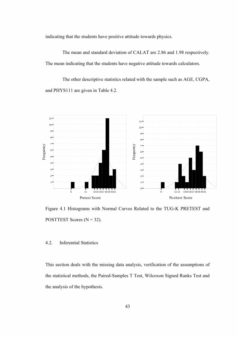
Figure 4.1 shows the histogram with the normal curves related to TUG-K
PRETEST and POSTTEST scores.
The mean and standard deviation of PHYSAT are 95.75 and 16.18
respectively. The PHYSAT was a 6 point likert-scale attitude test. The mean
43
indicating that the students have positive attitude towards physics.
The mean and standard deviation of CALAT are 2.86 and 1.98 respectively.
The mean indicating that the students have negative attitude towards calculators.
The other descriptive statistics related with the sample such as AGE, CGPA,
and PHYS111 are given in Table 4.2.
6 11 12 1415 1617 1819 2021
Posttest Score
0
1
2
3
4
5
6
7
8
9
10
11
Freq
uenc
y
6 11 1415 1617 1819 2021
Pretest Score
1
2
3
4
5
6
7
8
9
10
11
Freq
uenc
y
Figure 4.1 Histograms with Normal Curves Related to the TUG-K PRETEST and
POSTTEST Scores (N = 32).
4.2. Inferential Statistics
This section deals with the missing data analysis, verification of the assumptions of
the statistical methods, the Paired-Samples T Test, Wilcoxon Signed Ranks Test and
the analysis of the hypothesis.
44
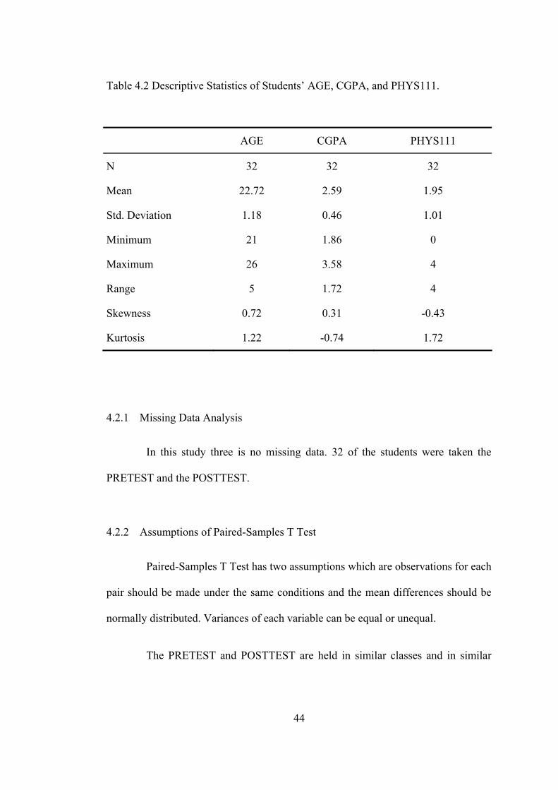
Table 4.2 Descriptive Statistics of Students’ AGE, CGPA, and PHYS111.
AGE CGPA PHYS111
N 32 32 32
Mean 22.72 2.59 1.95
Std. Deviation 1.18 0.46 1.01
Minimum 21 1.86 0
Maximum 26 3.58 4
Range 5 1.72 4
Skewness 0.72 0.31 -0.43
Kurtosis 1.22 -0.74 1.72
4.2.1 Missing Data Analysis
In this study three is no missing data. 32 of the students were taken the
PRETEST and the POSTTEST.
4.2.2 Assumptions of Paired-Samples T Test
Paired-Samples T Test has two assumptions which are observations for each
pair should be made under the same conditions and the mean differences should be
normally distributed. Variances of each variable can be equal or unequal.
The PRETEST and POSTTEST are held in similar classes and in similar

45
conditions to set the assumptions of the Paired-Samples T Test.
For normality assumption skewness and kurtosis values were used. The
values for skewness and kurtosis of PRETEST and POSTTEST scores were given in
Section 4.1. The skewness and kurtosis values except kurtosis of PRETEST can be
assumed in approximately acceptable range for a normal distribution.
4.2.3 Paired-Samples T Test
DV of the research is POSTTEST and the IV is PRETEST. As seen form
the Table 4.3 there is no significant effect of CBL on students’ understandings of
kinematics graphs.
Table 4.3 Paired-Samples T Test (N = 32)
Mean Std. Deviation
Std. Error Mean t df Sig. (2-tailed)
POSTTEST -PRETEST -0.59 2.434 0.43 -1.38 31 .178
4.2.4 Assumptions of Wilcoxon Signed Ranks Test
Wilcoxon Signed Rank Test is a nonparametric procedure used with two
related variables to test the hypothesis that the two variables have the same
distribution. It makes no assumptions about the shapes of the distributions of the two
variables.

46
4.2.5 Wilcoxon Signed Ranks Test
One may consider that the assumptions of the Paired-Samples T Test was
not achieved a nonparametric test must be used. The result of Wilcoxon Signed
Ranks Test indicated that there is no significant difference between PRETEST and
POSTTEST, z = - 1.13, p = 0.26. The mean of the negative ranks showing lower
score on POSTTEST was 15.68; the mean of the positive ranks showing higher score
on POSTTEST was 10.96.
4.2.4 Null Hypothesis
The Null Hypothesis was “there will be no significant effect of CBL on
students’ means of POSTTEST and PRETEST scores”.
Paired-Samples T Test was conducted to determine the effect of CBL on
students’ means of POSTTEST and PRETEST scores. As seen from the Table 4.3
the null hypothesis was accepted (t = -1.38, p = .178). There is no significant
difference between the students’ PRETEST and POSTTEST scores after the CBL
activities carried out.
4.3 Results of the Questionnaire: The Teacher Candidates’ Opinions about the
Treatment.
In this study, after the treatment the open – ended questions was given to 22
teacher candidates who are previously involved in the study. In the following part the
open – ended questions and the results of them are given in Table 4.4.

47
Table 4.4 Students’ Responses To Open – Ended Questions (N = 22)
Questions ScoreDif Students' responses to open - ended questions
Group %
Total %
The activities were very useful and enjoying 77,8 31,8
Students can see the results immediately which help them to understand better and makes the activities more concrete
55,6 22,7
This type of activities motivates the students 33,3 13,6 LO
W (N
= 9
)
The calculators were not simple to use 11,1 4,5 The activities were interesting. They will be very useful for high school students 57,1 18,2
This type of activities will be helpful for us when we become teachers 28,6 9,1
SAM
E (N
= 7
)
Students should also learn to draw graphics from the collected data 14,3 4,5
The activities were enjoying, interesting and useful 66,7 18,2
The apparatus were small and easy to install and conduct experiments 66,7 18,2
Wha
t is y
our o
pini
on a
bout
the
CB
L ac
tiviti
es a
nd th
e w
ays y
ou
like
and
disl
ike?
HIG
H (N
= 6
)
Students can see the results immediately this makes students easy to understand and motivate them
50,0 13,6
The POSTTEST was at the same day with our final exams 88,9 36,4
LO
W
(N =
9)
I may be careless at that time 22,2 22,2
We all know these subjects 85,7 27,3
SAM
E
(N =
7)
Some of us are not cared the activities 28,6 9,1
The graphs we were studied in the activities helped me answering questions 66,7 18,2
I have over come my misconceptions related with graphs 33,3 9,1
You
take
hig
her/l
over
/sam
e sc
ore
on P
OST
TEST
. W
hat a
re y
our o
pini
ons a
bout
this
resu
lt?
HIG
H (N
= 6
)
I do not think that my score was increased; I did one or two questions wrong unconsciously. 16,7 4,5

48
Table 4.4 (continued)
Questions ScoreDif Students' responses to open - ended questions
Group %
Total %
University entrance examinations (OSS – OYS) and the curriculum in high schools make us to study hard on these topics
88,9 36,4
LO
W (N
= 9
)
I teach these subjects 22,2 9,1
We have studied very hard on these topics while studying for University entrance examinations
85,7 27,3
SAM
E (N
= 7
)
Because we were physics students 14,3 4,5
We were studied on similar questions while studying for University entrance examinations
83,3 22,7
The
resu
lts o
f the
PR
ETES
T w
ere
muc
h hi
gher
than
the
expe
cted
va
lues
. (Th
e m
ean
of th
e te
st re
sults
of T
UG
– K
whi
ch w
as c
ondu
cted
in
USA
was
40
out o
f 100
. You
rs w
as 7
8 ou
t of 1
00).
Wha
t is t
he
reas
on o
f thi
s hig
h re
sult?
HIG
H (N
= 6
)
We were at a higher level 16,7 4,5
No 88,9 36,4
LO
W (N
= 9
)
I teach these subjects 11,1 4,5
SAM
E
(N =
7)
No 100,0 31,8
No 66,7 18,2
Hav
e yo
u ev
er st
udie
d on
a su
bjec
t whi
ch m
ay
affe
ct th
e re
sults
of P
RET
EST
afte
r you
hav
e ta
ken
PHY
S111
cou
rse?
HIG
H
(N =
6)
I teach these subjects 33,3 9,1

49
1) What is your opinion about the CBL activities and the ways you like
and dislike?
2) You take higher/lover/same score on POSTTEST. What are your opinions
about this result?
3) The results of the PRETEST were much higher than the expected values.
(The mean of the test results of TUG – K which was conducted in USA
was 40 out of 100. Yours was 78 out of 100). What is the reason of this
high result?
4) Have you ever studied on a subject which may affect the results of
PRETEST after you have taken PHYS111 course?
Students found the CBL activities useful, interesting and enjoying. Students
can see the results immediately this makes students easy to understand and this
motivates them. According to students the most probable reason of getting low
scores on POSTTEST was the time of the POSTTEST which was at the same time
with their finals. They found the questions of PRETEST easy because they were
familiar with them as they had solved similar questions while studying for university
entrance exams (OSS/OYS).
4.4 Summary of the Results
Parametric and nonparametric analysis of the test scores indicated that there
is no statistically significant difference between the PRETEST and POSTTEST

50
scores of the students. This result points to there is no effect of Calculator Based
Laboratories on students’ understandings of kinematical concepts. In order to find
out if there was an effect of CBL on some objectives of the test the test scores are
calculated according to objectives where the TUG – K has seven objectives so that
each student had seven scores on each test. A Paired-Samples T Test was carried out
to find out if there is a statistically significant difference between the objective scores
of the students’. The Table 4.5 describes that there is no statistically significant
change in students’ objective scores.
Table 4.5 Paired-Samples T Test of the TUG – K Objectives (N = 32)
Scores on TUK-G Mean SD Std. Error Mean Sig. (2-tailed)
POSTOBJ1 - PREOBJ1 0,03 0,74 0,131 0,813
POSTOBJ2 - PREOBJ2 -0,25 0,984 0,174 0,161
POSTOBJ3 - PREOBJ3 0,09 0,893 0,158 0,557
POSTOBJ4 - PREOBJ4 -0,31 0,965 0,171 0,077
POSTOBJ5 - PREOBJ5 -0,22 0,751 0,133 0,109
POSTOBJ6 - PREOBJ6 -0,06 0,716 0,127 0,625
POSTOBJ7 - PREOBJ7 -0,19 0,78 0,138 0,184
Final calculations made to find out if there are any statistically significant
correlations between students SCOREDIF and PHYS111, PHYSAT, CALAT and
ACTSCORE. Correlation coefficients were computed among the five variables. The
results of the correlational analysis are presented in the Table 4.6. None of the four

51
correlations were statistically significant with p values grater than .01 (Bonferroni
approach was used to control Type I error across the correlations between five
variables).
Table 4.6 Partial Correlations among the IVs of the Study
PHYS111 PHYSAT CALAT ACTSCORE
SCOREDIF -,02 -,27 -,13 -,07
Analysis of open – ended questions showed that most of the students
believed that the activities are useful and interesting. The most probable result that
affects the significance of the study is the time of the POSTTEST which was
conducted in the same time with the final exams of the students. Most of the
opinions of the students are the TUG – K questions are similar with the questions of
university entrance examinations this caused a high mean score in PRETEST. And
most of them said that they did not studied similar subjects after they have taken
PHYS111 course.

52
CHAPTER 5
CONCLUSIONS, DISCUSSION AND IMPLICATION
The purpose of this study was to investigate the effects of Calculator Based
Laboratories (CBL) on students’ understandings of kinematics graphs. To achieve
this purpose, this chapter is given in six sections. The conclusions are given in the
first section. The discussion of the results is given in the second section. Internal and
external validity are given in the third and the fourth section respectively. The fifth
section comprises implications of the study. Finally in the last section,
recommendations for further studies are introduced.
5.1. Conclusions
The sample of the study chosen from accessible population was a sample of
convenience. Consequently there is a limitation about the generalizability of this
study. On the other hand the conclusions presented beneath can be applied to a
broader population of similar students.
The Calculator Based Laboratory Activities was not affecting students’
understandings of kinematics graphs. So we can conclude that Calculator Based
Laboratory Activities did not increase the level students’ understandings of
kinematics graphs.

53
5.2. Discussion of the Results
Findings of this study implied that there is no significant effect of the
Calculator Based Laboratories on students’ understandings of kinematics graphs.
The students POSTEST mean was 17.19 out of 21 questions it was very high with
respect to Beicher’s findings which was 8.4. Depending on these high scores it was
hard to improve students’ scores on POSTTEST. Besides that the POSTTEST was
administered at the final dates of the students which may be another reason of
students’ getting lover scores on POSTTEST. All students in the sample were
physics teacher candidates. This might also lead students to take high scores on
PRETEST.
Thornton et al. (1990) warn that the tools themselves are not enough but
that gains in learning appear to be produced by a combination of the MBL devices
and appropriate curricular material that guides the students to examine appropriate
phenomena. MBL use multiple modalities, pair events in real time with their
symbolic representations, provide scientific experiences similar to those of scientists
in actual practice, and eliminate the drudgery of graph production. These were the
reasons why MBL technology is useful according to Mokros et al. (1987). They also
suggest that encouraging collaboration is an added benefit of MBL. For motion
phenomena, using simultaneous graph production to link a graph with a physical
concept seems to be essential.
Although the literature suggests benefits from using MBL technology, we
must also consider problems that may arise if we do not pay attention to how the

54
technology is implemented. Some studies indicate that without proper precautions,
technology can become an obstacle to understanding (Lapp et al., 2000).
Future research also should address how students view the authority of
technology in problem solving. Research suggests that we can be optimistic about
the benefits of MBL and CBL use in forming graphical concepts. However, it is too
early to draw final conclusions. Further study is needed before the research
community can make any definitive statements on the pedagogical advantages of
data collection devices.
Similar studies showed that this type of activities increases the students’
level of understandings. Students believe that these activities are useful. They also
believe that the scores on POSTTEST that they got would be higher if the test was
not administered at the same time with their final examinations.
5.3. Internal Validity
Internal validity of a study means that the observed differences on the
dependent variable are related with the independent variable, not some other
unintended variables which are not controlled (Fraenkel & Wallen, 2003). In this
section possible threats to internal validity and the methods used to manage them are
discussed.
As known from the previous studies some subject characteristics such as
previous cumulative grade point average, age, gender, and physics attitudes might

55
affect students’ difference in PRETEST and POSTTEST scores. However they are
not used in statistical analysis because there is no statistically significant effect of
CBL on students’ difference between PRETEST and POSTTEST scores. Students’
cognitive development, mathematical skills, and problem solving skills can also be
mentioned as effective variables affecting internal validity.
Other variables such as history, maturation, instrument decay, data collector
characteristics, data collectors’ bias, testing, statistical regression, attitude of subjects
and implementation may have effect on the dependent variables as mentioned in
Frankel et. al. 2003.
Besides the other variables history threat might affect the results of the
study. History may be a threat when an unplanned event occurs (Frankel et. al.
2003). In this study students’ final dates and the posttest date are coincided. This
may explain why students didn’t do well in posttest.
The study was completed in 4 weeks. As a result maturation of the subjects
shouldn’t be a threat to internal validity of the study.
There were 32 subjects which were involved in the study. The instrument
was a multiple choice type test so the nature of the instrument did not change. So
instrument decay threat to internal validity was controlled.
Data collector characteristics, data collector bias and implementation should
not be threat for the study since there was one data collector, he was the researcher
himself, and the data collection procedure was standardized.

56
In order to minimize the effects of testing threat the time difference between
the POSTTEST and the PRETEST is more than 3 weeks, approximately 4 weeks. It
would be better if the POSTTEST questions were different but identical to
PRETEST questions or at least an alternate test of which questions modified. For
example, graph scales were shifted slightly, graphed lines were made superficially
steeper or flatter, etc (Beichner, 1994).
One another threat to internal validity is statistical regression. In this study
because of the time limitations and the convenience of the sample the physics teacher
candidates were involved in the study which has higher achievement scores on the
subject of the study. This may explain why there is no statistically significant
between PRETEST and POSTTEST scores.
In order to eliminate the effect of attitudes of subjects to the internal validity
is to make students to believe that the treatment is just a regular part of their
instruction (Frankel et. al. 2003).
The names of the students were taken for the sake of statistical analyses.
And these data are not used in any forms. As a result confidentiality wouldn’t be a
problem for this study.
5.4. External Validity
Population Generalizability: The population generalizability refers to the
degree to which a sample of study represents the population of interest (Frankel &

57
Wallen, 1996).
Ecological Generalizability: The ecological generalizability is the degree to
which the results of a study can be extended to other settings or conditions (Frankel
& Wallen, 1996). For this study, the treatments and testing procedure took in place in
ordinary classrooms in the education faculty during regular class time. Therefore, the
results of the study can be generalized to similar cases.
5.5. Implications
According to results of the study it couldn’t be shown the effectiveness of
the Calculator Based Laboratories. But it doesn’t mean that that the CBL is
ineffective. In the light of previous studies on the same topic, the effectiveness of
CBL/MBL the following suggestions can be offered.
As Beichner (1994) suggested he first step is for teachers to become aware
of the problem. The major problem of the students’ is inability to use graphs as
"fluently" as they should. Students need to understand graphs before they can be
used as a language for instruction. Teachers should have students examine motion
events where the kinematics graphs do not look like photographic replicas of the
motion and the graph lines do not go through the origin. Students should be asked to
translate from motion events to kinematics graphs and back again. Instruction should
also require students to go back and forth between the different kinematics graphs,
inferring the shape of one from another. Teachers should have students determine
slopes and areas under curves and relate those values to specific times during the

58
motion event. All these suggestions for modifying instruction can be summarized by
one phrase-teachers should give students a large variety of "interesting" motion
situations for careful, graphical examination and explanation. The students must be
given the opportunity to consider their own ideas about kinematics graphs and then
encouragement to help them modify those ideas when necessary. Teachers cannot
simply tell students what the graphs' appearance should be. These suggested ways
can be simply conducted with CBL Activities.
Further suggestions can be listed as follows:
1. Teachers should prepare themselves to carry out CBL activities. They
should improve themselves about how to encourage their students to
perform CBL activities and how to make physics more exiting for them.
They should also know how to cooperate with administrators and gain
their support and encouragement.
2. Administrators of school should investigate the possibilities of using
CBL activities in their schools and then support these efforts.
3. Universities should evaluate the strengths and weaknesses, and develop
lessons including CBL activities, pre-service and in-service workshops.
4. Curriculum developers should require the use of CBL activities as
standard part of physics instruction.
5. Educators must replace teaching methods that hinge on rote
memorization with genuine experiences like CBL activities.

59
5.6. Recommendations for Further Research
For the further studies the followings can be suggested.
1. Further studies could investigate the effects of CBL on improving
students’ understanding and interpretation of kinematics graphs with a
control group and a sample which gives higher opportunity no
generalize the results of the study.
2. Future research could perform a replication of the current study with a
larger, more diverse sample.
3. Future research could investigate the effects of CBL in different physics
topics, different science subjects and different grade levels.
4. Future research could use extra assessment strategies, observational
checklists and portfolios in order to extend the analysis.
5. Future research could perform a replication of this study for a longer
time that is integrated in the flow of physics course.
6. Future research could investigate the change in the students’ levels of
understandings of graphics by using Palms instead of using Calculators.

60
REFERENCES
Adams, T. L. (1997). Addressing students' difficulties with the concept of function:
Applying graphing calculators and a model of conceptual change. Focus on
Learning Problems in Mathematics, 19 (2), 43 – 57.
Adie, G. (1998). The impact of the graphics calculator on physics teaching. Physics
Education, 33, 50 – 54.
Arkin H. & Colton R. R. (1940). Graphs, how to make and use them (5th Ed.) New
York & London.
Arons, A.B. (1983) Student patterns of thinking and reasoning: part one of three
parts, The Physics Teacher, 21, 576–581.
Ates, S. & Truman, J. S. (2003). Teaching Line Graphs to Tenth Grade Students
Having Different Cognitive Developmental Levels by Using Two Different
Instructional Modules. Research in Science & Technological Education, 21
(1), 55 – 66.
Beichner, J, R. (1990). The effects simultaneous motion representation and graph
generation in a kinematics laboratory. Journal of Research in Science
Teaching, 27 (8), 803 – 815.
Beichner, J, R. (1994). Testing students’ interpretation of kinematics graphs.
American Journal of Physics, 62 (8), 750 – 762.

61
Berg, C. A. & Philips, D.G. (1994). An investigation of the relationship between
logical thinking and the ability to construct and interpret line graphs.
Journal of Research in Science Teaching, 31 (4), 323 – 344.
Brasell, H. (1987). The effects of real-time laboratory graphing on learning graphic
representations of distance and velocity. Journal of Research in Science
Teaching, 24 (4), 385 – 395.
Curriculum Administrator (1997). Science teachers are making connections with
students using Texas Instruments Calculator – Based Laboratory trade mark
system. Curriculum Administrator, 3 (17), 4 – 5.
Dick, T. & Dunham, P. H. (2000). Kinematics and Graphs: Students’ difficulties and
CBLs. The Mathematics Teacher, 93 (5), 414 – 417.
Doerr, H. M. & Rieff, C. (1999). Putting Math in Motion with Calculator-Based
Labs. Mathematics Teaching in the Middle School, 4 (6), 364 – 367.
Dunham, P. H. & Osborne, A. (1991). Learning how to see: Students’ graphing
difficulties. Focus on Learning Problems in Mathematics, 13 (4), 35–49.
Dunham, P. H. (1993). Does using calculators work? The jury is almost in. UME
Trends, 5 (2), 8-9.
Dunham, P. H., & Dick, T. P. (1994). Research on graphing calculators.
Mathematics Teacher, 87, 440 – 445.
Dunham, P. H. D., Thomas P. (1994). Connecting research to teaching: research on
graphing calculators. Mathematics Teacher, 87 (6), 440 – 445.

62
Dunham, P. H. (1996). Looking for trends: What's new in graphing calculator
research? In G. Goodell (Ed.), Proceedings of the Eighth International
Conference on Technology in Collegiate Mathematics 120-124. Reading,
MA: Addison-Wesley.
Educational Technology & Calculators. Retrieved December, 11th 2002 from World
Wide Web: http://education.ti.com/educationportal/
Ersoy, Y. (2003). Teknoloji destekli matematik öğretimi – II: Hesap makinelerin
matematik etkinliklerinde kullanımı. İlköğretim On – Line, 2 (2), 35 – 60.
Forinash, K. & Wisman, R. (2001). Science Laboratories. T H E Journal, 29 (2), 38 –
43.
Fraenkel, J. R., & Wallen, N. E. (2003). How to design and evaluate research in
science education. (5th Ed.) NY. McGraw – Hill, Inc.
Fey, J. T., Hirsch, C. R. (1992). Calculators in mathematics education. Reston, Va.:
National Council of Teachers of Mathematics.
Goldberg, F. M., & Anderson, J. H. (1989). Student Difficulties with Graphical
Representations of Negative Values of Velocity. The Physics Teacher 27,
254 – 60.
Goldenberg, E. P., Harvey, W., Lewis, P. G., Umiker, R. J., West, J., & Zodhiates, P.
(1988). Mathematical, technical, and pedagogical challenges in the
graphical representation of functions (Tech. Rep. No. 88-4). Cambridge,
MA: Harvard University, Educational Technology Center.
63
Hale, P. L. (1996). Building conceptions and repairing misconceptions in student
understanding of kinematics graphs: Using student discourse in Calculator-
Based Laboratories (Doctoral dissertation, Oregon State University).
Dissertation Abstracts International, 57, 08A.
Hardal O. (2003). The effects of hands – on activities on students’ achievement and
attitudes towards physics. Unpublished Master Thesis, Middle East
Technical University, Ankara.
Hegarty, E. (1987) Science laboratory teaching, in: M. J. DUNKIN (Ed.)
International Encyclopedia of teaching and Teacher Education (Oxford,
Pergamon Press).
Henderson, D. & Fisher, D. (1998). Assessing Learning Environments in Senior
Science Laboratories. Australian Science Teachers Journal, 44 (4), 57 – 62.
Hennessy, S. (1999). The potential of portable technologies for supporting graphing
investigations. British Journal of Educational Technology, 30 (1), 57-60.
Jones, P. L. (1993). Realizing the educational potential of the graphics calculator. In
L. Lum (Ed.), Proceedings of the Sixth International Conference on
Technology in Collegiate Mathematics, 212-217. Reading, MA: Addison-
Wesley.
Kwon, O. N. (2002). The effect of calculator based ranger activities on students’
graphing ability. School Science and Mathematics 102 (2), 57 – 67.
Lapp D. A., Cyrus, V. F., Dick, T., Dunham, P. H. (2000). Using Data – Collection
Devices to Enhance Students’ Understanding. Mathematics Teacher, 93 (6),
504 – 510.

64
Lauten, A. D., Graham, K., & Ferrini-Mundy, J. (1994). Student understanding of
basic calculus concepts: Interaction with the graphics calculator. Journal of
Mathematical Behavior, 13, 225 – 237.
Leinhardt, G., Zaslavsky, O., and Stein, M. K. (1990). Functions, graphs, and
graphing: Tasks, learning, and teaching. Review of Educational Research,
60 (1), 1 – 64.
Linn, M. C. (1988). Perspectives for research in science teaching: Using the
computer as laboratory partner. Paper presented at the European
Conference for Research on Learning, Tubingen, West Germany,
September 19–22, 1987. (ERIC Document Reproduction Service No. ED
308 853)
Linn, M. C., & Songer, N. B. (1988). Curriculum reformulation: Incorporating
technology into science instruction. Paper presented at the annual meeting
of the American Educational Research Association, New Orleans, LA,
April 1988. (ERIC Document Reproduction Service No. ED 303 352)
Linn, M.C., Layman, W.J. & Nachmias, R. (1987) Cognitive consequences of
microcomputer based laboratories: graphing skills development,
Contemporary Educational Psychology, 12, 244–253.
McDermott, L. C., Rosenquist M. L. & Van Zee E. H. (1987). Student difficulties in
connecting graphs and physics: Examples from kinematics. American
Journal of Physics, 55 (6), 503 – 513.

65
Meltzer, D. E. (2003).The Questions We Ask and Why: Methodological Orientation
in Physics Education Research. Retrieved December, 19th 2003 from
World Wide Web:
http://www.physics.iastate.edu/per/docs/Meltzer_PERC_2003_paper.pdf
Mokros, J. R. & Tinker, J. F. (1987). The impact of microcomputer based
laboratories on children’s’ ability to interpret line graphs. Journal of
Research in Science Teaching, 24 (4), 369 -383.
McKenzie, D. L. & Padilla, M. J. (1986). The construction and validation of The
Test of Graphing in Science (TOGS). Journal of Research in Science
Teaching, 23 (7), 571 – 579.
Michael, T.S. (1995). Effect of microcomputer based laboratory on graphing
interpretation skills and understanding of motion. Paper presented at the
annual meeting of the National Association of Research in Science
Teaching, San Francisco, CA.
Nachmias, R. & Linn, M. C. (1987). Evaluations of science laboratory data: The role
of computer presented information. Journal of Research in Science
Teaching, 24 (5), 491 – 506.
Norman, F. A. (1993). Integrating research on teachers' knowledge of functions and
their graphs: Integrating research on the graphical representation of
functions. Integrating research on the graphical representation of functions,
159 - 187. Hillsdale, NJ. Lawrence Erlbaum Associates.
Olme, A. (2000). Views on the physics curriculum beyond 2000. Physics Education,
35 (3), 195 – 198.
66
Padilla, J.M., McKenzie, L.D. & Shaw, L.E., JR. (1986). An examination of line
graphing ability of students in grades seven through twelve, Scholl Science
& Mathematics, 86, 20–26.
Penglase, M., & Arnold, S. (1996). The graphics calculator in mathematics
education: A critical review of recent research. Mathematics Education
Research Journal, 8, 58 – 90.
Pomerantz H. (1997). The role of calculators in math education. Urban Systemic
initiative/comprehensive partnership for mathematics and science
achievement superintendents’ forum, Dallas, Texas.
Quesada, A. R. M., Mary E. (1994). The effects of using graphing calculators to
enhance college students' performance in Precalculus. Educational Studies
in Mathematics, 27 (2), 205-15.
Redish, E. F. (1993). What can a physics teacher do with a computer? Invited talk
presented at Robert Resnick Symposium RPI, Troy NY, May, 1993.
Redish, E. F., Steinberg, R., Saul, J. (1997). On the effectiveness of active-
engagement microcomputer – based laboratories. American Journal of
Physics, 65 (1), 45 – 54.
Rieff, C., Doerr, H. M., & Tabor, J. (1999). Putting Math in Motion with Calculator-
Based Labs, Mathematics Teaching in the Middle School, Mar 1999, 364 –
367.
Saeki, A., Ujiie, A., & Tsukihashi, M. (2001). A cross – curricular integrated
learning experience in mathematics and physics. Community College
Journal of Research and Practice 25, 417 – 424.

67
Sancar, M. (2002). Unpublished lecture notes. Project on Science Teaching.
Svec, M.T. (1995, April) Effect of Micro-Computer based laboratory on graphing
interpretation skills and understanding of motion. Paper presented at the
Annual Meeting of the National Association for Research in Science
Teaching, San Francisco (ERIC Document Reproduction Service No. ED
383 551).
Svec, M.T. (1999). Improving graphing interpretation skills and understanding of
motion using microcomputer based laboratories. Retrieved May, 13th 2001
from World Wide Web: http://unr.edu/homapage/crowther/ejse/svec.html
Taylor, L.R. (1995). Using the graphing calculator – in physics labs. The physics
Teacher 33, (5), 312 – 319.
The On – Line Education Center. Science in the New Zealand curriculum. Retrieved
October, 23rd 2003 from World Wide Web:
http://www.tki.org.nz/r/science/curriculum/p9_e.php
Thornton, R. K. & Sokoloff, D. R. (1990). Learning motion concepts using real –
time microcomputer based laboratories. American Journal of Physics, 58
(9), 858 – 867.
Tobin, K. (1990) Research on science laboratory activities: in pursuit of better
questions and answers to improve learning, School Science and
Mathematics, 90, 403-418.
Trumper, R. (2002). What Do We Expect From Students’ Physics Laboratory
Experiments? Journal of Science Education and Technology, 11 (3), 221 –
228.

68
Svec, M.T. (1995) Effect of Micro-Computer based laboratory on graphing
interpretation skills and understanding of motion. Paper presented at the
Annual Meeting of the National Association for Research in Science
Teaching, San Francisco
Welker, J. (1999). Using technology to teach sciences. Media & Methods, 36, 63.

69
APPENDICES
APPENDIX A
OBJECTIVE LIST
Students will be able to:
1. determine velocity from the given position - time graph
2. determine acceleration from the given velocity-time Graph
3. determine displacement from the given velocity - time graph
4. determine change in velocity from the given acceleration - time graph
5. select another corresponding graph from the given kinematics graph
6. select textual description from the given kinematics graph
7. select corresponding graph from the given textual motion description

70
APPENDIX B
TEST OF UNDERSTANDING GRAPHS – KINEMATICS (TUG – K)

71
Test of Understanding Graphs − Kinematics version 2.6
Instructions
Wait until you are told to begin, then turn to the next page and begin working. Answer each question as accurately as you can. There is only one correct answer for each item. Feel free to use a calculator and scratch paper if you wish.
Use a #2 pencil to record your answers on the computer sheet, but please do not write in the test booklet.
You will have approximately one hour to complete the test. If you finish early, check over your work before handing in both the answer sheet and the test booklet.
©1996 by Robert J. Beichner North Carolina State University Department of Physics Raleigh, NC 27695-8202 [email protected]

72
1. Velocity versus time graphs for five objects are shown below. All axes have the
same scale. Which object had the greatest change in position during the interval?
Time0
(A)
Time0
(B)
Time0
(C)
Time0
(D)
Time0
(E)
yticoleV
yticoleV
yticoleV
yticoleV
yticoleV
2. When is the acceleration most negative?
(A) RtoT
(B) TtoV
Time
yticoleV
0
Q R S T U V W X Y Z
(C) V
(D) X
(E) XtoZ
3. To the right is a graph of an object's motion. Which
sentence is the best interpretation?
Time0
noitisoP
(A) The object is moving with a constant, non-zero acceleration.
(B) The object does not move.
(C) The object is moving with a uniformly increasing velocity.
(D) The object is moving with a constant velocity.
(E) The object is moving with a uniformly increasing acceleration.

73
4. An elevator moves from the basement to the tenth floor of a building. The mass of
the elevator is 1000 kg and it moves as shown in the velocity-time graph below.
How far does it move during the first three seconds of motion?
(A) 0.75 m
(B) 1.33 m
(C) 4.0 m
(D) 6.0 m
(E) 12.0 m
0 1 2 3 4 5 6 7 8 9 100
1
2
3
4
5
Time (s)
)s/m(
yticoleV
5. The velocity at the 2 second point is:
(A) 0.4 m/s
(B) 2.0 m/s
(C) 2.5 m/s
(D) 5.0 m/s
(E) 10.0 m/s
.
0 1 2
)m(
noitisoP
3 40
5
10
15
Time (s)5

74
6. This graph shows velocity as a function of time for a car of mass 1.5 x 10³ kg.
What was the acceleration at the 90 s mark?
(A) 0.22 m/s2
(B) 0.33 m/s2
(C) 1.0 m/s2
(D) 9.8 m/s2
(E) 20 m/s2
.
0 30 60 90 120 1500
10
20
30
40
Time (s)180)s/
m(yticole
V
7. The motion of an object traveling in a straight line is represented by the following
graph. At time = 65 s, the magnitude of the instantaneous acceleration of the object
was most nearly:
(A) 1 m/s2
(B) 2 m/s2
(C) +9.8 m/s2
(D) +30 m/s2
(E) +34 m/s2
0 20 40 60 80 1000
10
20
30
40
Time (s)
)s/m(
yticoleV
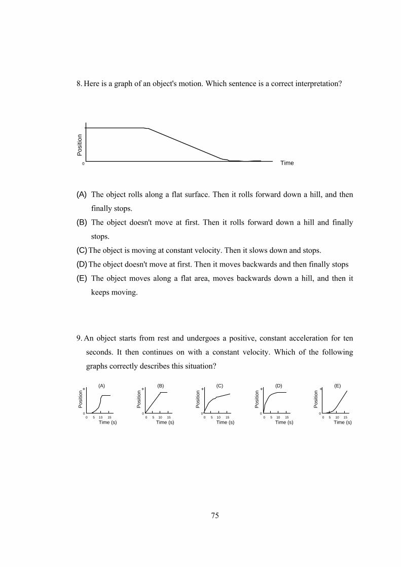
75
8. Here is a graph of an object's motion. Which sentence is a correct interpretation?
Time
noitisoP
0
(A) The object rolls along a flat surface. Then it rolls forward down a hill, and then
finally stops.
(B) The object doesn't move at first. Then it rolls forward down a hill and finally
stops.
(C) The object is moving at constant velocity. Then it slows down and stops.
(D) The object doesn't move at first. Then it moves backwards and then finally stops
(E) The object moves along a flat area, moves backwards down a hill, and then it
keeps moving.
9. An object starts from rest and undergoes a positive, constant acceleration for ten
seconds. It then continues on with a constant velocity. Which of the following
graphs correctly describes this situation?
Time (s)
noitisoP
0
(A)
noitisoP
0
(B)
noitisoP
0
(C)
noitisoP
0
(D)
noitisoP
0
(E)+++++
Time (s) Time (s) Time (s) Time (s)0 5 10 15 0 5 10 15 0 5 10 15 0 5 10 15 0 5 10 15

76
10. Five objects move according to the following acceleration versus time graphs.
Which has the smallest change in velocity during the three second interval?
Time (s)0
(A)
0
(B)
0
(C)
0
(D)
0
(E)
5
3
5
3
s/m(
noitareleccA
2 )
5
3
s/m(
noitareleccA
2 )
5
3
s/m(
noitareleccA
2 )
5
3
s/m(
noitareleccA
2 )s/m(
noitareleccA
2 )
Time (s) Time (s) Time (s) Time (s)
11. The following is a position-time graph for an object during a 5 s time interval.
Time (s)
noitisoP 0
+
1 2 3 4 5
–
Which one of the following graphs of velocity versus time would best
represent the object's motion during the same time interval?
Time (s)
yticoleV
0
+
1 2 3 4 5
–
(A)
Time (s)
yticoleV
0
+
1 2 3 4 5
–
(B)
Time (s)
yticoleV
0
+
1 2 3 4 5
–
(C)
Time (s)
yticoleV
0
+
1 2 3 4 5
–
(E)
Time (s)
yticoleV
0
+
1 2 3 4 5
–
(D)

77
12. Consider the following graphs, noting the different axes:
Time0
(I)
0
(II)
0
(III)
0
(IV)
0
(V)
yticoleV
yticoleV
noitareleccA
noitareleccA
Time Time Time Time
noitisoP
Which of these represent(s) motion at constant velocity?
(A) I, II, and IV
(B) I and III
(C) II and V
(D) IV only
(E) V only
13. Position versus time graphs for five objects are shown below. All axes have
the same scale. Which object had the highest instantaneous velocity during the
interval?
.
Time0
(A)
Time0
(B)
Time0
(C)
Time0
(D)
Time0
(E)noitisoP
noitisoP
noitisoP
noitisoP
noitisoP

78
14. The following represents a velocity-time graph for an object during a 5 s time
interval.
Time (s
yticoleV
0
+
1 2 3 4 5
–
Which one of the following graphs of
acceleration versus time would best
represent the object's motion during the
same time interval?
Time (s)
noitareleccA 0
+
1 2 3 4 5
–
(A)
Time (s)
noitareleccA 0
+
1 2 3 4 5
–
(B)
Time (s
noitareleccA 0
+
1 2 3 4 5
–
(C)
Time (s)0
+
1 2 3 4 5
–
(E)
Time (s)0
+
1 2 3 4 5
–
(D)noitareleccA
noitareleccA
15. The following represents an acceleration graph for an object during a 5 s time
interval.
0 1 2
)s/m(
yticoleV
3 40
5
10
15
Time (s)5
Which one of the following graphs of
velocity versus time would best represent
the object's motion during the same time
interval?
Time0
(I)
0
(II)
0
(III)
0
(IV)
0
(V)
yticoleV
yticoleV
noitareleccA
noitareleccA
Time Time Time Time
noitisoP

79
16. An object moves according to the graph below:
The object's change in
velocity during the first
three seconds of motion
was: 0 1 2 3 4 5 6 7 8 9 10
0
1
2
3
4
Time (s
)s/m(
yticoleV
(A) 0.66 m/s (B) 1.0 m/s (C) 3.0 m/s (D) 4.5 m/s (E) 9.8 m/s
17. The velocity at the 3 second point is about:
(A) -3.3 m/s
0 1 2 3 4 0
5
10
15
Pos
ition
(m)
5
(B) -2.0 m/s
(C) -.67 m/s
(D) 5.0 m/s
(E) 7.0 m/s
Time (s)
18. Consider the following graphs, noting the different axes:
Time0
(I)
0
(II)
0
(III)
0
(IV)
0
(V)
yticoleV
yticoleV
noitareleccA
noitareleccA
Time Time Time Time
noitisoP
Which of these represent(s) motion at constant, non-zero acceleration?
(A) I, II, and IV (B) I and III (C) II and V (D) IV only (E) V only

80
0 1 2
/m(
yticoleV
3 40
5
10
15
Time (s)5
)s
0 Time
yt icoleV
19. If you wanted to know the distance
covered during the interval from t = 0 s
t=2s, from the graph below you would:
(A) Read 5 directly off the vertical axis
(B) Find the area between that line segment and the time axis by calculating (5 x 2)/2
(C) Find the slope of that line segment by dividing 5 by 2.
(D) Find the slope of that line segment by dividing 15 by 5.
(E) Not enough information to answer.
20. An object moves according to the graph below:
How far does it move during the interval from t=4 s to t = 8s?
0 1 2 3 4 5 6 7 8 9 100
1
2
3
4
Time (s
)s/m(
yticoleV
(A) 0.75 m (B) 3.0 m (C) 4.0 m (D) 8.0 m (E) 12.0 m
21. To the right is a graph of an object's motion. Which
sentence is the best interpretation?
(A) The object is moving with a constant acceleration
(B) The object is moving with a uniformly decreasing acceleration.
(C) The object is moving with a uniformly increasing velocity.
(D) The object is moving at a constant velocity.
(E) The object does not move.

81
Answers: 1. B
2. E
3. D
4. D
5. C
6. B
7. A
8. D
9. E
10. A
11. D
12. B
13. D
14. B
15. A
16. D
17. A
18. B
19. C
20. E
21. A

82
APPENDIX C
CBL ACTIVITIES
ACTIVITY 1 (Graphics Matching)
Aktivite 1 - Grafik Eşleştirme:
Amaç: Hesap makinesi tarafından verilen konum – zaman grafiklerini eşleştirmek.
Araç ve Gereçler: Grafik hesap makinesi (TI – 83 Plus), CBL ve sonik mesafe ölçer (CBR).
Yöntem ve Data Toplama:
1) Bir elinize CBR diğer elinize de hesap makinesini alın. CBR ‘yi direkt olarak
duvara yönlendirin.
İpucu: Verilen grafiklerde en yakın mesafe 0,5 m en uzak mesafe de 4
m.dir.
2) Hesap makinesinin APPS tuşuna basın.CBL/CBR uygulamasından,
RANGER programını çalıştırın.
3) MAIN MENU den APPLICATIONS ve METERS seçeneğini seçin.
4) APPLICATIONS dan DISTANCE MATCH i seçin.
5) Hesap makinesinin ENTER tuşuna basarak eşleştirme yapacağınız grafiği
seçin. Bir süre grafiğin üzerinde düşünün daha sonra 1 ve 2. soruların
cevaplarını verin.

83
6) Grafiği değerlendirerek duvardan uzaklığınızı belirleyiniz. ENTER tuşuna
basarak ölçümü başlatın. CBR üzerindeki yanıp sönen yeşil ışık datanın
toplandığını gösterir.
7) İleri ve geri yürüyerek verilen grafiğe eşdeğer bir grafik elde etmeye çalışın.
Konumunuz ekranda görünecektir.
8) Ölçüm bitiğinde grafiklerin ne kadar eşleştiğine bakın ve 3. soruya cevap
verin.
9) Gerekirse ENTER tuşuna basarak OPTIONS dan SAME MATCH i seçerek
eşleştirmenizi daha iyi hale getirin.
10) 4, 5 ve 6. sorulara cevap verin.
Gözlemler:
Grafik eşleştirmelerinde grafik 3 doğru parçasından oluşmaktadır.
1) ENTER tuşuna basarak OPTIONS dan NEW MATCH ı seçin. İlk doğru
parçasını seçerek 7 ve 8. sorulara cevap verin.
2) Tüm grafiği gözden geçirerek 9 ve 10. sorulara cevap verin.
3) ENTER tuşuna basarak grafiği eşleştirmeye çalışın.
4) 11 ve 12. sorulara cevap verin.
5) ENTER tuşuna basarak OPTIONS dan NEW MATCH ı seçin.
6) Grafiği değerlendirerek 13, 14 ve 15. soruları cevaplandırın.

84
Sorular:
1) X-ekseninde hangi fiziksel değer gösterilmekted
Birimi nedir?__________________________________
Y-ekseninde hangi fiziksel değer gösterilmektedi
Birimi nedir? _________________________________
2) Harekete duvardan ne kadar mesaf
düşünüyorsunuz? _____________________________
3) Başlangıç noktanız doğrumuydu? _______________
kadar hata yaptınız? __________________________
4) Eğim yukarı doğruysa ileri mi yoksa geri
Neden?_______________________________________
5) Eğim aşağı doğruysa ileri mi yoksa geri
Neden?_______________________________________
6) Eğim düz ise ileri mi yoksa geri m
Neden?_______________________________________
Adı Soyadı:
ir? _____________
________________
r? ______________
________________
eden başlamayı
________________
Eğer değilse ne
________________
mi yürümelisiniz?
________________
mi yürümelisiniz?
________________
i yürümelisiniz?
________________

85
7) Her saniyede 1 adım atıyorsanız her adımda kaç metre yol almanız
gerekir? _____________
8) Her adımını 1 metre ise saniyede kaç adım atmalısınız?
________________________________
9) Hangi doğru parçasında hızınız en fazla idi? Neden?
______________________________________________________________
10) Hangi doğru parçasında hızınız en az idi? Neden?
______________________________________________________________
11) İleri yada geri yürümeye karar verirken başka hangi faktörler sizin
için etkili oldu? _______________________________________________
12) Doğru parçalarının eğimi hangi fiziksel değeri vermektedir?
______________________________________________________________

86
13) İlk doğru parçası için kaç saniyede kaç metre yürümeniz gerekti?
______________________________________________________________
14) 13. sorudaki değeri metre/saniye ‘ye çevirin. ____________________
metre/dakika ________________________________________________
metre/saat __________________________________________________
kilometre/ saat _______________________________________________
15) Grafiği eşleştirmek için kaç metre yürüdünüz? __________________

87
ACTIVITY 2 (Constant Velocity)
Aktivite 2 - Oyuncak Araba (Sabit Hızlı Hareket):
Amaç: Sabit hızla hareket eden cisimlerin incelenmesi.
Araç ve Gereçler: Grafik hesap makinesi (TI – 83 Plus), CBL, sonik mesafe ölçer (CBR), ray ve araba.
Yöntem ve Data Toplama:
1) Arabayı CBR den en az 15 cm ileriye yerleştirin.
2) Data toplamaya başlamadan önce 1. soruyu cevaplandırın.
3) Ranger programını çalıştırın.
4) MAIN MENU den SETUP/SAMPLE ı seçin ve aşağıdaki ayarlamaları
yapın.
NO 5 SECONDSDISTANCE[ENTER] LIGHT METER
REALTIME:TIME(S):
DISPLAY:BEGIN ON:
SMOOTHING:UNITS:
5) START NOW a basın.
6) Hazır olduğunuzda ENTER tuşuna basın ve arabayı hareket ettirin.
7) Data toplama bittiğinde hesap makinesi otomatik olarak Konum-Zaman
grafiğini çizecektir.

88
8) 1. soruda vermiş olduğunuz cevap ile sonucu karşılaştırın benzerlik ve
farklılıkları değerlendirin.
Gözlemler:
1) 1. soruda verilen tabloya grafikten elde ettiğiniz verileri girin.
2) 3 ve 4. sorulara cevap verin.
3) Her zaman dilimindeki konum değişimlerini hesaplayın.
4) Daha sonra eğimi hesaplayarak tabloya yazın.
5) 5, 6 ve 7. sorulara cevap verin.

89
Sorular: 1) Arabanın Konum-Zaman grafiği sizce aşağıdakileolacaktır?
Neden? __________________________________ 2)
Zaman Konum ∆ Konum ∆ Zama
1 xxx xxx
1,5
2
2,5
3
3,5
4
4,5
5
Adı Soyadı:
rden hangisi gibi
____________________
n m
xxx
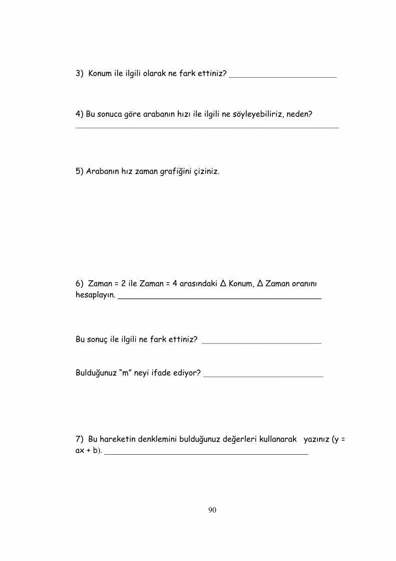
90
3) Konum ile ilgili olarak ne fark ettiniz? ___________________________ 4) Bu sonuca göre arabanın hızı ile ilgili ne söyleyebiliriz, neden? __________________________________________________________________ 5) Arabanın hız zaman grafiğini çiziniz. 6) Zaman = 2 ile Zaman = 4 arasındaki ∆ Konum, ∆ Zaman oranını hesaplayın. ___________________________________________________ Bu sonuç ile ilgili ne fark ettiniz? ______________________________ Bulduğunuz “m” neyi ifade ediyor? ______________________________ 7) Bu hareketin denklemini bulduğunuz değerleri kullanarak yazınız (y = ax + b). ___________________________________________________

91
8) Araba eğer hareketine devam etseydi 10 saniye içinde ne kadar hareket ederdi? ______________________________________________ 9) 10 dakika içinde ne kadar hareket ederdi? _____________________

92
ACTIVITY 3 (Constant Acceleration I)
Aktivite 3 – Oyuncak Araba (Düzgün Hızlanan Hareket)
Amaç: Düzgün hızlanan cisimlerin incelenmesi.
Araç ve Gereçler: Grafik hesap makinesi (TI – 83 Plus), CBL, sonik mesafe ölçer (CBR), ray ve araba.
Yöntem ve Data Toplama:
1) Data toplamaya başlamadan önce 1. soruyu cevaplandırın.
2) DataMate programını çalıştırın. SETUP tan MODE u seçin. TIME
GRAPH ı seçin ve aşağıdaki ayarları yapın.
TIME INTERVAL: .05 NUMBER OF SAMPLES: 100 EXPERIMENT LENGHT: 5
3) START a basarak deneyi başlatın. CBR data almaya başladığında arabayı
serbest bırakın.
4) DIG – DISTANCE ı seçerek Konum – Zaman, DIG – VELOCITY ı
seçerek Hız – Zaman, DIG – ACCELERATION ı seçerek de İvme – Zaman
grafiğini inceleyebilirsiniz. Eğer gerekliyse RESCALE den grafiklerin
minimum ve maksimum değerlerini ayarlayabilirsiniz. SELECT REGION
dan hesaplarınızı yapacağınız zaman aralığını belirleyebilirsiniz.
5) Konum – Zaman grafiğini inceleyin, 2, 3, 4 ve 5. soruları cevaplandırın.

93
Gözlemler:
6) Eğer eğik düzlemin açısını artırırsak Konum – Zaman grafiği nasıl olur,
cevabınızı 6. soruda verilen grafiğe çizin.
7) Eğik düzlemin açısını arttırarak deneyi tekrarlayın.
8) Eğer eğik düzlemin açısını 0o sonrada 90o ye ayarlamış olsaydık Konum –
Zaman grafikleri nasıl olurdu? Tahminlerinizi 7. soruda verilen tabloya
çizin.
Gelişmiş Gözlemler:
ANALYZE dan CURVE FIT i seçin. Daha sonra da uygun seçeneği seçin. 8 ve
9. sorulara cevap verin.

94
Sorular:
1) Arabanın Konum-Zaman grafiği sizce aşağıdakiler
olacaktır?
2) X-ekseninde hangi fiziksel değer gösterilmektedi
Birimi nedir? _________________________________
Y-ekseninde hangi fiziksel değer gösterilmektedir
Birimi nedir? _________________________________
3) Elde ettiğiniz grafiği aşağıdaki tabloya çizip ekse
beraber adlandırın. Arabanın eğik düzlemin başınd
bulunduğu yerleri grafikte gösteriniz.
Adı Soyadı:
den hangisi gibi
r? ______________
________________
? ______________
________________
nleri birimleriyle
a ve sonunda
95
4) Bu grafik nasıl bir fonksiyonudur? ______________________________
5) 1. soruya vermiş olduğunuz cevap ile deney sonucunda elde
ettiğiniz grafiğin benzerlik ve farklarını tartışın.
______________________________________________________________
______________________________________________________________
6) Eğik düzlemin açısı arttırıldığında grafik nasıl olacak, aşağıdaki
tabloya çizin.

96
7) Eğer eğik düzlemin açısını 0o sonrada 90o ye ayarlamış olsaydık
Konum – Zaman grafikleri nasıl olurdu?
8) Hesaplama sonucunda elde ettiğiniz sabitler hangi fiziksel
değerleri ifade etmektedir? ___________________________________
______________________________________________________________
9) Hareketin denklemini yazınız. __________________________________
10) Bulduğunuz değerlere göre hareketin hız – zaman ve ivme – zaman
grafikerini çiziniz.

97
ACTIVITY 4 (Constant Acceleration II)
Aktivite 4 – Oyuncak Araba (Newton Dinamiği):
Amaç: Hesap makinesi tarafından verilen konum – zaman grafiklerini eşleştirmek.
Araç ve Gereçler: Grafik hesap makinesi (TI – 83 Plus), CBL, sonik mesafe ölçer (CBR), ray, çeşitli
ağırlıklar, ip ve araba.
Yöntem ve Data Toplama:
1) Deney düzeneğini kurun. Arabayı çekmesi için 5 gramlık ağırlığı yerleştirin
ve toplam kütleyi belirleyin.
2) Data toplamaya başlamadan önce 1. soruyu cevaplandırın.
3) DataMate programını çalıştırın. SETUP tan MODE u seçin. TIME
GRAPH ı seçin ve aşağıdaki ayarları yapın.
TIME INTERVAL: .05
NUMBER OF SAMPLES: 100
EXPERIMENT LENGHT: 5
4) START a basarak deneyi başlatın. CBR data almaya başladığında arabayı
serbest bırakın.
5) DIG – DISTANCE ı seçerek Konum – Zaman, DIG – VELOCITY ı
seçerek Hız – Zaman, DIG – ACCELERATION ı seçerek de İvme – Zaman
grafiğini inceleyebilirsiniz. Eğer gerekliyse RESCALE den grafiklerin

98
minimum ve maksimum değerlerini ayarlayabilirsiniz. SELECT REGION
dan hesaplarınızı yapacağınız zaman aralığını belirleyebilirsiniz. 2, 3, 4, 5 ve
6. soruları cevaplandırın.
6) Toplam kütleyi 2 katına çıkaracak şekilde arabanın üzerine ağırlık koyun ve
ölçümleri tekrar yapın. 7. soruyu cevaplandırın.
7) Arabayı çeken kütleyi 5 gramdan 10 grama çıkarın ve ölçümleri tekrar yapın.
8. soruyu cevaplandırın.

99
Sorular:
1) Arabanın Konum-Zaman grafiği sizce aşağıdak
olacaktır?
1) X-ekseninde hangi fiziksel değer gösterilmekt
Birimi nedir? ______________________________
Y-ekseninde hangi fiziksel değer gösterilmekt
Birimi nedir? ______________________________
2) Elde ettiğiniz grafiği aşağıdaki tabloya çizip e
beraber adlandırın. Arabanın düzlemin başında
bulunduğu yerleri grafikte gösteriniz.
Adı Soyadı:
ilerden hangisi gibi
edir? ______________
___________________
edir? ______________
___________________
ksenleri birimleriyle
ve sonunda

100
3) Bu grafik nasıl bir fonksiyonudur? ______________________________
4) 1. soruya vermiş olduğunuz cevap ile deney sonucunda elde
ettiğiniz grafiğin benzerlik ve farklarını tartışın.
______________________________________________________________
______________________________________________________________
5) ANALYZE dan CURVE FIT i seçin. Daha sonra da uygun seçeneği
seçin. Elde ettiğiniz sabitler hangi fiziksel değerleri ifade
etmektedir? __________________________________________________
Hareketin denklemini yazınız. __________________________________
6) Elde ettiğiniz denklemdeki sabitleri kullanarak arabanın hız –
zaman ve ivme zaman grafiklerini çiziniz.

101
7) Toplam kütle iki katına çıktığında hareket nasıl değişti? __________
Hareketin denklemini yazınız. __________________________________
8) Arabayı çeken kütle iki katına çıktığında hareket nasıl değişti? _____
Hareketin denklemini yazınız. __________________________________
9) Hareketin ivmesi ile arabayı çeken kütle arasında nasıl bir ilişki
buldunuz? ___________________________________________________

102
APPENDIX D
OBJECTIVE - ACTIVITY TABLE
Activity
Objective Act. 1 Act. 2 Act. 3 Act. 4
1 X X
2 X X
3 X X
4 X
5 X
6 X X
7 X X

103
APPENDIX E
PHYSICS ATTITUDE TEST
Adı Soyadı:
Bölüm:
GPA:
CGPA:
ÖSS (giriş yılı ile beraber):
Fizik 111 notunuz:
Babanızın Eğitim Düzeyi
a) İlk b) Orta c) Lise d) Üniversite e) Yüksek Lisans
Annenizin Eğitim Düzeyi
a) İlk b) Orta c) Lise d) Üniversite e) Yüksek Lisans
Babanızın Mesleği:
Annenizin Mesleği:
Kardeş sayınız :
Kardeşlerinizin eğitim düzeyleri:
a) İlk b) Orta c) Lise d) Üniversite e) Yüksek Lisans
Okumakta olduğunuz bölüm kaçıncı tercihinizdi?

104
Bu bölümü tercih etme sebebiniz nedir (isteyerek yada puanınız tuttuğu
için)?
Bu bölüme gelmeseydiniz hangi bölümde okumak isterdiniz?
Aldığınız dersler içinde en ilgili olduğunuz hangileridir?
Aldığınız dersler içinde en güçlük çektiğiniz dersler hangileridir?
Sizin için En Uygun olan Cevabı İşaretleyin:
1)Kesinlikle Katılmıyorum 6)Kesinlikle Katılıyorum
1) Fizik dersi benim için angaryadır. 1 2 3 4 5 62) Fizik dersi beni huzursuz eder. 1 2 3 4 5 63) Fizik dersi beni ürkütür. 1 2 3 4 5 64) Fizik dersinden hoşlanmam. 1 2 3 4 5 65) Fizik dersi bütün dersler içinde en korktuğum derstir. 1 2 3 4 5 66) Fizik dersi benim için ilgi çekicidir. 1 2 3 4 5 67) Fizik sevdiğim bir derstir. 1 2 3 4 5 68) Fizik dersi benim için ilgi çekicidir. 1 2 3 4 5 69) Fizik dersi olmasa öğrencilik hayatı daha ilgi çekici olur. 1 2 3 4 5 610) Derslerim içinde en sevimsizi Fizik dersidir. 1 2 3 4 5 611) Fizik dersi sınavından çekinirim. 1 2 3 4 5 612) Fizik dersinde zaman geçmek bilmez. 1 2 3 4 5 613) Arkadaşlarımla Fizik konularını tartışmaktan zevk alırım. 1 2 3 4 5 614) Fiziğe ayrılan ders saatlerinin daha fazla olmasını dilerim. 1 2 3 4 5 615) Fizik dersi çalışırken canım sıkılır. 1 2 3 4 5 616) Yıllarca fizik okusam bıkmam. 1 2 3 4 5 617) Diğer derslere göre fiziği daha çok severek çalışırım. 1 2 3 4 5 618) Fizik dersinde neşe duyarım. 1 2 3 4 5 619) Fizik dersi eğlenceli bir derstir. 1 2 3 4 5 620) Çalışma zamanımın çoğunu fiziğe ayırmak isterim. 1 2 3 4 5 6
105
APPENDIX F
CALCULATOR ATTITUDE TEST Adı Soyadı: Aşağıdaki sorula kendiniz için en uygun olan cevabı veriniz. evet hayır1) Günlük çalışmalarınızda ve/veya işinizde Hesap Makinelerini
kullanır mısınız? 2) Hesap Makinelerini kullanmada yeterli bilgi/deneyiminiz var
mı? 3) Hesap Makineleri ve bilgisayar konusunda kitap/yayınları okur
musunuz? 4) Hesap Makineleri ve bilgisayar ile ilgili gelişmeler ilginizi
çeker mi? 5) Bazı Hesap Makineleri ile ilgili olarak ayrıntılı bilgi edinmek
ister misiniz? 6) Kendinizin bir Hesap Makinesi olsun ister misiniz? 7) Hesap Makineleri ile ilgili bir seminere katılmak ister misiniz? 8) Hesap Makineleri Fizik derslerinde kullanılsın mı? 9) Fizik derslerinde Hesap Makinelerinin kullanılması fiziksel
kavramların öğrenilmesinde yardımcı olur mu?

106
APPENDIX G
QUESTIONNAIRE: TEACHER CANDIDATES’ OPINIONS ABOUT
THE TREATMENT
Adı Soyadı:
Gecen Mayıs ayı içerisinde yapmış olduğumuz Hesap Makineleri destekli laboratuar
(HeMa Lab) etkinlikleri ile ilgili yapacağımız analiz ve değerlendirmeleri daha
sağlıklı bir şekilde yapabilmemiz için aşağıdaki sorulara cevap vermenizi istiyoruz.
Katkılarınız için teşekkür ederim.
1) Yapmış olduğumuz HeMa Lab etkinlikleri ile ilgili görüşleriniz, beğendiğiniz ve
beğenmediğiniz yönleri nelerdir?
2) Uygulamış olduğumuz testlerde başarınızın azaldığını/değişmediğini/arttığını
gördük. Sizce bunun sebepleri neler olabilir.
3) Uygulamış olduğumuz testte sonuçlarına göre başarı ortalamanız 100 üzerinden 78 çıktı (Bu test
Amerika uygulandığında başarı % 40 çıkmış). Sizce bunun sebepleri neler olabilir?
4) Lisans eğitiminiz boyunca; size uygulamış olduğumuz testte başarınızı etkileyebilecek
bir çalışmanız yada almış olduğunuz bir ders oldu mu (Phys 111 haricinde) ?

107
APPENDIX H
RAW DATA
NO GENDER LGPA CGPA FGPA PHYS111 AGE FED 1 1 2,9 2,9 3,1 2 21 3 2 0 2,6 2,7 1 0 23 0 3 1 2,2 2,4 1,4 0 23 4 4 0 2,8 3,2 3,5 4 22 3 5 1 3,2 2,7 2,1 2 23 3 6 0 2,5 2,5 2,8 4 21 2 7 0 1,9 2,4 1,9 2 23 0 8 1 2,2 2,3 1,3 2 22 3 9 1 2,7 3,1 1,5 2 22 0 10 1 3,2 3,3 2,3 3 23 2 11 1 1,1 2,1 1,8 3 23 3 12 1 3,6 2,9 2,5 3 21 1 13 1 2,3 2,4 0,95 1 21 3 14 0 1,5 2 2,2 2 26 3 15 0 2,2 2,4 1,3 3 23 0 16 0 1,1 2 1,4 3 23 4 17 1 1,4 2 0,32 0 24 3 18 0 2,6 3,3 0,84 0 23 0 19 0 1,2 1,9 1,2 2 25 1 20 1 1,9 2,5 2,4 2 22 0 21 0 3,5 3,6 3,8 4 23 1 22 0 2,6 2,8 1,3 2 23 0 23 1 3 2,8 3,4 2 23 0 24 0 2,8 2,5 1,4 2 25 2 25 1 2,8 3,2 2 3 23 2 26 1 2,3 2,6 1,5 2 21 3 27 0 2,5 3 3,5 3 23 3 28 0 2,7 2,4 1,6 2 23 1 29 1 3,3 2,8 2,2 2 22 0 30 0 1,1 2 1,3 3 22 0 31 1 1,8 2,1 1,2 2 22 0 32 0 1,4 2,2 0,39 2 23 0
108
NO MED NC PREF REASON PHYSAT CALAT ACTSCORE
1 3 2 6 1 65 10 91,22
2 0 2 11 0 69 9 76,5
3 4 2 1 0 70 16 61,67
4 3 1 14 1 65 12 66,89
5 3 1 9 1 77 9 71,72
6 2 1 9 0 62 10 85,56
7 0 2 8 1 71 13 60,61
8 3 2 6 1 71 13 68,56
9 0 5 7 2 58 11 57,39
10 0 1 11 1 56 12 74,22
11 2 1 16 1 67 11 71,5
12 0 2 4 1 76 12 85,06
13 2 1 17 0 47 12 61,11
14 2 1 5 0 52 9 63,06
15 1 1 9 1 50 16 46,83
16 1 1 3 3 59 11 62,61 17 3 2 18 0 75 10 56,39 18 0 2 3 0 68 10 82,22 19 2 1 13 0 45 13 44,5 20 0 2 5 0 62 12 78,56 21 0 1 , 0 63 14 76,89 22 0 1 12 0 63 11 78,39 23 0 2 8 1 61 13 58,89 24 0 2 9 0 66 12 73,06 25 0 2 1 0 70 9 80,67 26 3 1 8 4 63 10 70,89 27 1 1 12 1 58 16 59,89 28 0 2 11 1 70 12 86,39 29 3 1 4 0 75 13 67,72 30 0 0 10 1 51 14 64 31 0 1 5 1 76 12 84,83 32 0 3 13 0 49 13 74,78

109
NO PRETEST POSTTEST SCOREDIF1 17 16 -1 2 18 18 0 3 17 11 -6 4 21 21 0 5 19 17 -2 6 19 18 -1 7 20 19 -1 8 11 12 1 9 15 17 2
10 19 21 2
11 21 20 -1
12 16 12 -4
13 17 17 0
14 17 18 1
15 19 14 -5
16 20 20 0
17 6 6 0
18 21 19 -2
19 16 19 3
20 17 19 2
21 19 20 1
22 19 14 -5
23 14 16 2 24 16 16 0 25 15 12 -3 26 18 16 -2 27 19 16 -3 28 19 20 1 29 16 12 -4 30 17 20 3
31 14 15 1
32 18 20 2

110
NO preobj1 preobj2 preobj3 preobj4 preobj5 preobj6 preobj7
1 3 1 3 2 2 3 3
2 2 2 2 3 3 3 3
3 2 2 3 3 2 3 2
4 3 3 3 3 3 3 3
5 2 3 3 2 3 3 3 6 3 2 3 3 3 3 2 7 3 3 3 3 2 3 3 8 0 0 3 2 1 1 2 9 1 2 3 3 2 2 2
10 2 3 3 2 3 3 3
11 3 3 3 3 3 3 3
12 1 2 2 2 3 3 2
13 2 3 3 3 2 3 2
14 2 2 2 3 2 2 3 15 3 2 3 2 3 3 3 16 3 2 3 3 3 3 3 17 1 1 0 0 1 1 2 18 3 3 3 3 3 3 3 19 2 2 3 2 3 2 2 20 3 2 3 2 2 3 2 21 3 2 3 3 3 3 2 22 2 3 3 3 3 3 2 23 1 1 3 3 2 1 3 24 2 3 1 2 3 3 2 25 2 1 3 2 3 2 2 26 2 3 3 2 3 2 3 27 3 2 3 3 3 3 3 28 3 3 3 2 3 3 2 29 1 3 3 2 3 1 3 30 2 3 2 3 2 3 3
31 2 1 3 3 2 1 2
32 3 3 3 3 2 3 3

111
NO postobj1 postobj2 postobj3 postobj4 postobj5 postobj6 postobj7
1 2 2 3 2 2 2 3
2 2 3 3 2 2 3 3
3 2 0 2 2 2 2 2
4 3 3 3 3 3 3 3
5 2 3 3 2 2 3 2
6 3 2 3 2 3 3 2
7 2 3 2 3 3 2 2
8 2 0 3 1 2 2 3
9 2 2 3 3 3 2 2
10 3 2 3 3 3 3 3
11 2 1 3 3 3 3 3
12 1 1 2 0 3 3 2
13 2 3 3 2 2 3 1
14 3 3 3 2 2 3 1
15 2 2 2 2 2 3 1
16 2 3 3 3 3 3 3
17 0 1 0 0 2 2 1
18 3 3 2 3 2 1 3
19 3 1 3 3 3 3 3
20 3 2 3 3 2 3 3 21 3 3 3 3 3 2 3 22 1 1 3 2 3 3 2 23 2 2 3 3 1 2 3 24 2 1 2 3 3 3 2 25 2 2 3 1 2 2 1 26 2 1 3 3 1 2 3 27 3 2 2 1 1 2 2 28 3 2 3 3 3 2 2 29 1 2 3 1 2 1 2 30 3 3 3 3 2 3 3 31 2 1 3 0 2 2 3 32 3 3 3 3 2 3 2

112