the effects of inflation targeting on economic …
TRANSCRIPT

THE EFFECTS OF INFLATION TARGETING ON ECONOMIC GROWTH IN SOUTH
AFRICA
By
MOKGOLA AUBREY
Dissertation submitted in fulfilment for the degree of
Master of Commerce
in
ECONOMICS
In the
FACULTY OF MANAGEMENT AND LAW
School of Economics and Management
at the
UNIVERSITY OF LIMPOPO
Supervisor: Prof R Ilorah
Co-Supervisor: Mr S Zhanje
2015

ii
DECLARATION
I declare that the dissertation hereby submitted to the University of Limpopo, for the
degree of master of commerce in economics has not previously been submitted by me
for a degree at this or any other university; that it is my work in design and in execution,
and that all material contained herein has been duly acknowledged.
Mokgola A (Mr) : 31 December 2014

iii
ACKNOWLEDGMENTS
I wish to extend my sincere gratitude to all those who have assisted me in completing
this thesis materially, logistically and through word of advice or otherwise.
Firstly, I would like to thank God Almighty for protecting and guiding me throughout the
research and writing of this dissertation. If it were not for Him, this would not have been
possible.
To my supervisors, Prof Richard Ilorah and Mr Stephen Zhanje, thank you for your
supervision and encouragements through the completion of this dissertation. May God
bless you.
Finally, I would like to thank everyone who supported me directly or indirectly until the
finish line of my dissertation. May God richly bless you.

iv
ABSTRACT
South Africa is among a number of countries that have adopted inflation targeting as
their monetary policy framework since 1990. This policy was adopted in the year 2000
in South Africa, and there have been a growing number of concerns about the effects of
inflation targeting on economic growth in South Africa. The main purpose of this study
is to determine these effects of inflation targeting on economic growth in South Africa. In
this paper, the author used co-integration and error correction model to empirically
examine the long-run and short-run dynamics of inflation targeting effects on economic
growth. A final conclusion that inflation targeting does not have significant negative
effects on economic growth is drawn from two interesting results. Firstly, there is an
insignificant negative relationship between inflation targeting and economic growth.
Secondly, the influence that inflation targeting has on the relationship between the lag of
inflation and economic growth is also insignificant. These findings have important policy
implications. Therefore, the critique that the SARB achieves relatively low inflation at the
expense of low economic growth is a misconception. This led to the conclusion that the
SARB should maintain its monetary policy framework of inflation targeting which has
helped it to reduce inflation.
Keywords: Inflation targeting, inflation, economic growth, error correction model,
monetary policy.

v
TABLE OF CONTENTS
Declaration ............................................................................................................ii
Acknowledgements ...............................................................................................iii
Abstract .................................................................................................................iv
List of Tables .........................................................................................................viii
List of Figures ........................................................................................................ix
CHAPTER 1: INTRODUCTION
1.1 Introduction ................................................................................................1
1.2 Research Problem ......................................................................................3
1.3 Hypotheses.................................................................................................4
1.4 Research Questions ...................................................................................4
1.5 Purpose of the Study ..................................................................................5
1.5.1 Aim...................................................................................................5
1.5.2 Objectives ........................................................................................5
1.6 Rationale and Motivation for the Study .......................................................4
CHAPTER 2: ECONOMIC GROWTH ...................................................................6
2.1 Defining Economic Growth .........................................................................6
2.2 Theories of Economic Growth ...................................................................6
2.2.1 The Solow-Sawn Growth Model ......................................................6
2.2.2 Endogenous Growth Theory ............................................................7
2.2.3 Classical Growth Theory ..................................................................7
2.3 Inflation Targeting Countries’ Growth Experience ......................................8
2.4 South African Growth Experience ...............................................................11
CHAPTER 3: INFLATION .....................................................................................13
3.1 Define inflation .............................................................................................13
3.2 Theories of Inflation .....................................................................................13
3.2.1 Keynesian Theory ............................................................................13
3.2.2 Money and Monetarism....................................................................15
3.3 Why Does Inflation Matter? .........................................................................16
3.4 What Causes Inflation ..................................................................................17

vi
3.5 Controlling Inflation ......................................................................................19
3.6 Inflation and Economic Growth Trade-Off ....................................................20
3.7 Inflation, Growth and Central Bank (SARB) .................................................22
CHAPTER 4: INFLATION TARGETING ................................................................23
4.1 Measuring Inflation Targeting ......................................................................23
4.1.1 Specifying the Target .......................................................................24
4.1.2 Who Sets the Target ........................................................................24
4.2 Rationale for Inflation Targeting ...................................................................25
4.3 The Flexibility of Inflation Targeting .............................................................25
4.4 Critiques of Inflation Targeting .....................................................................26
4.5 Economic Growth and Inflation Targeting ....................................................28
CHAPTER 5: METHODOLOGY ............................................................................30
5.1 Introduction ..................................................................................................30
5.2 Research Design .........................................................................................30
5.3 Research Setting .........................................................................................31
5.4 Research Populations and Sampling ...........................................................31
5.5 Data ............................................................................................................31
5.5.1 Data sources ....................................................................................32
5.6 Data Analysis ...............................................................................................32
5.7 Model Specification ......................................................................................32
5.8 Econometric Techniques .............................................................................33
5.8.1 The Long-Run Relationship .............................................................33
5.8.2 Augmented Engle-Granger Approach [AEG] ...................................34
5.8.3 Error Correction Model [ECM] ..........................................................35
5.8.4 Diagnostic Tests ..............................................................................35
5.8.5 Stability Tests ...................................................................................36
5.8.6 Hypothesis Testing ..........................................................................36
5.8.7 The Null Hypothesis .........................................................................37
5.8.8 The Alternative Hypothesis ..............................................................37
5.8.9 The Test Statistics ...........................................................................37

vii
5.8.10 Significant Testing ............................................................................38
5.8.11 Confidence Interval ..........................................................................38
5.8.12 Correlation .......................................................................................39
5.8.12.1 The R2 ............................................................................39
5.8.12.2 Adjusted R2 ....................................................................40
5.8.12.3 F Test .............................................................................40
5.9 Conclusion ...................................................................................................40
CHAPTER 6: DATA INTERPRETATION AND RESULTS DISCUSSION .............41
6.1 Introduction ..................................................................................................41
6.2 Unit Root Test with Graphs ..........................................................................41
6.2.1 The Graphical Representation of Economic Growth ......................41
6.2.2 Graphical Representation of Inflation Rate ....................................43
6.2.3 Graphical Representation of Interest Rates ...................................44
6.2.4 Graphical Representation of Unemployment Rate .........................45
6.3 Unit Root Test Results .................................................................................46
6.4 The Long-Run Relationship .........................................................................48
6.5 Co-Integration Test Results: Augmented Engle-Granger ............................48
6.6 Error Correction Model ................................................................................49
6.7 Diagnostic Tests ..........................................................................................50
6.8 Stability Tests ..............................................................................................51
6.9 Average Output and Output Variability ........................................................52
6.10 Conclusion.................................................................................................52
CHAPTER 7: CONCLUSION AND RECOMMENDATIONS ..................................53
7.1 Introduction .................................................................................................53
7.2 Conclusions from Theoretical Perspective ...................................................53
7.3 Conclusions from the Findings of the present study ....................................54
7.4 Limitations of the Study ...............................................................................56
7.5 Future Research ..........................................................................................56
7.6 Recommendations .......................................................................................57

viii
LIST OF TABLES
Table 6.1: Results of Unit Roots Tests ..................................................................47
Table 6.2: Results of Long Run Relationship ........................................................48
Table 6.3: Co-Integration Test Results ..................................................................49
Table 6.4: Results of Error Correction-Model ........................................................50
Table 6.5: Results from Diagnostic Tests ..............................................................51
Table 6.6: Results of Stability Test ........................................................................52
Table 6.7: Mean and Variability .............................................................................52

ix
LIST OF FIGURES Figure 3.1 The Keynesian Theory .........................................................................14
Figure 3.2 The effect of an increase in the money supply according to
the monetarists ......................................................................................................16
Figure 3.3: Demand Pull Inflation ..........................................................................18
Figure 3.4: Cost Push Inflation ..............................................................................19
Figure 3.3: The Phillips Curve ...............................................................................20
Figure 6.1A: Economic Growth in Level Form (Y) ................................................42
Figure 6.1B: Economic Growth at First Difference (DY) ........................................42
Figure 6.2A: Inflation in Level form (X) ..................................................................43
Figure 6.2B: Inflation at First Difference (DX) ........................................................43
Figure 6.3A: Real Interest Rates in Level Form (R) .............................................44
Figure 6.3B: Real Interest Rates at First Difference (DR) .....................................44
Figure 6.4A: Unemployment Rate in Level Form (U) ............................................45
Figure 6.4B: Unemployment Rate at First Difference (DU) ...................................45

1
CHAPTER 1
INTRODUCTION AND BACKGROUND
1.1 INTRODUCTION
A growing number of countries have adopted inflation targeting as their monetary
policy framework since 1990. According to Brimmer (2002), there are more than 30
countries using an inflation targeting monetary policy framework. Inflation targeting
has sometimes been criticised for being ‘inflation only’ centred but ignoring economic
growth considerations. Bernanke (2003) on the other hand, has argued that the idea
of inflation targeting focusing exclusively on control of inflation and ignoring output
and employment objectives is a misconception. It is therefore crucial at this stage to
provide a clear and brief explanation about this policy before going into details.
Inflation targeting refers to an economic policy in which the Central Bank estimates
and announces in public a targeted inflation rate, and then attempts to steer the
actual inflation towards the targeted range through the use of interest rate changes
and other monetary policy instruments (Mishkin, 2000). According to Mishkin (2006),
“inflation targeting is a recent monetary policy strategy that includes five main
elements:
the public announcement of medium-term numerical targets for inflation;
an institutional commitment to price stability as the primary goal of monetary
policy, to which other goals are subordinated;
an information inclusive strategy in which many variables, and not just
monetary aggregates or the exchange rate, are used for deciding the setting
of policy instruments;
increased transparency of the monetary policy strategy through
communication with the public and markets about the plans, objectives, and
decisions of the monetary authorities; and
increased accountability of the Central Bank for attaining its inflation
objectives”.
Therefore, inflation targeting entails more than the announcement of a numerical
target over a specific time horizon. In a study of inflation targeting for Turkey, Civcir

2
and Akcaglayan (2010) have found that the adoption of inflation targeting has
increased the credibility of the Central Bank of Turkey.
In setting an inflation target a decision has to be made about the level of the target.
According to Van der Merwe (2004) the target can be specified in terms of a range, a
single point or a ceiling. A fixed single point target is much more difficult to achieve
than a range or ceiling. A range or ceiling leaves some discretion to the Central
Bank and can provide flexibility in the case of unforeseen price shocks. In South
Africa, the initial target range of 3 to 6 percent was set by the Minister of Finance in
consultation with the SARB. South Africa thus opted for a target range rather than a
point target and in February 2000 the Minister of finance announced publicly that
formal inflation targeting was to be adopted in the country as the monetary policy
framework (Van den Heever, 2001).
There is no obvious theoretical consensus that inflation targeting could affect output
growth. Although there is no theoretical and empirical consensus about the overall
impact of inflation targeting on output growth, it is accepted that all inflation targeting
Central Banks “not only aim at stabilizing inflation around the target but also put
some weight on stabilizing the real economy” (Svensson, 2007). On the other hand,
some economists argue that inflation has a global negative impact on medium and
long-run economic growth (Kormendi & Meguire, 1985; Barro, 1991; Chari et al.,
1996; and Gylfason & Herbertsson, 2001). However, the common view is that
inflation targeting does affect inflation behaviour which then lays a foundation for
economic growth. There is an indirect relationship between inflation targeting and
economic growth. The adoption of a monetary policy framework that focuses
explicitly on inflation is a realisation that, to promote economic growth in South
Africa, the authorities must maintain a low and stable inflation rate. Low and stable
inflation is supportive of high and stable long-term growth and a monetary policy
supportive of long-run growth can be viewed as more credible (Sarel, 1996).
There has been a growing concern about the use of inflation targeting by SARB as
its monetary policy framework. There have been questions about the extent to which
inflation targeting affects economic growth in South Africa. For example, inflation
targeting has been a source of political debate between the African National

3
Congress (ANC) government and its allies in the South African Communist Party
(SACP) and trade union movements (COSATU). The SACP and COSATU argue
that inflation targeting has negative impacts on economic growth and that it should
therefore be abolished. Instead they propose that the SARB commitment should be
on employment stability (Mboweni, 2006).
However, the Central Banks of many countries (such as New Zealand, Mexico,
Egypt and Australia among others) have pursued inflation targeting since the 1990s
and evidence shows that the policy has in general resulted in the reduction of the
inflation rate (Petursson, 2004). During the implementation of inflation targeting if
inflation appears to be above the target range the Central Bank is more likely to raise
interest rates, and if inflation is below the target the Central Bank is more likely to
reduce the interest rates (ibid). These actions by the Central Bank are aimed at
maintaining price stability in the interest of balanced and sustainable economic
growth over time.
1.2 Research Problem
There are conflicting opinions and disagreements amongst politicians, professionals,
labour organizations and economists about whether inflation targeting has a
favourable or unfavourable impact on economic growth in South Africa. Because
money can affect many economic variables that are important to the well-being of
our economy, politicians and policy makers throughout the world care about the
conduct of monetary policy, the management of money and interest rates (Mishkin,
2010). For example, the Finance Minister (Pravin Gordhan) has argued that South
Africa should keep its policy of targeting inflation, which has helped to stabilize prices
and encourage economic growth, whereas the labour organization (COSATU)
argued that inflation targeting leads to overemphasis of monetary stability at the cost
of growth and development (COSATU, 2007). The extent to which the pursuit for
inflation targeting exerts measurable influences on economic growth (real GDP) is
therefore the main concern in this study.
Previous studies have attempted to address inflation targeting related problems by
comparing the average level and fluctuations of real output between inflation

4
targeting countries and non-inflation targeting countries. For instance, Batini and
Laxton (2006) and the IMF (2006) have provided positive evidence about the
performance of inflation targeting regimes in developing countries, with lower
inflation rates and less volatile inflation and output growth. To the best of my
knowledge the study of how inflation targeting affects the level of real output growth
in the context of a single semi-developed country such as South Africa has not yet
been carried out and therefore the need for this study arises.
1.3 Hypothesis
The relevant null and alternative hypotheses include:
H0: the Inflation targeting monetary policy framework as employed in South
Africa does not significantly influence economic growth.
H1: the Inflation targeting monetary policy framework as employed in South
Africa does significantly influence economic growth.
1.4 Research Questions
Research questions investigated include the following:
How does inflation-targeting affect economic growth?
Does inflation targeting reduce or promote economic growth in South Africa?
What differences may exist between output growth variability prior and after
inflation targeting?
What are the challenges facing the inflation targeting objective to ensure
stable inflation, while maintaining high and stable long-term economic growth?
What can be done to ensure high and stable long-term economic growth at
the same time keeping inflation rate within the target range?
1.5 Purpose of the Study
1.5.1 Aim
The purpose is to determine the effects of inflation targeting on economic growth in
South Africa. It is hoped that our findings might help to reconcile disagreements,
resolve conflicts and clarify existing speculations and uncertainties among

5
politicians, labour organizations and policy makers about how inflation targeting
affects economic growth.
1.5.2 Objectives of the Study
To explore the effects of inflation targeting on economic growth.
To determine whether inflation targeting reduces or promotes economic
growth in South Africa.
To determine whether inflation targeting leads to high or low variations in the
level of economic growth.
To identify the challenges facing inflation targeting monetary policy framework
objective to ensure stable inflation, while maintaining high and stable long-
term economic growth in South Africa.
To find out whether inflation targeting is conducive for high and stable long-
term economic growth in South Africa as a semi-developed country.
1.6 Rationale and Motivation for the Study
The motivation for this study is to contribute to the existing body of knowledge in
economic theories and empirical studies on inflation targeting. The problem
addressed in this study concerns the lack of studies or information that focus on the
effects of inflation targeting on economic growth for a specific country. It is noted in
section 1.2 that studies such as that of Batini and Laxton (2006) and IMF (2006)
have found inflation targeting to have positive effects on economic growth. However,
these studies do not give adequate information on its effects on a specific country. It
could be that the negative effects of inflation targeting in some countries within the
chosen sample was smoothed out by higher positive economic growth in other
countries within the sample. In view of the afore-mentioned, this study attempts to
address this gap in knowledge.

6
CHAPTER 2
ECONOMIC GROWTH
2.1 Defining Economic Growth
There are numerous definitions of economic growth. For instance, Solow (1956)
defines economic growth as the increase in the amount of goods and services
produced by the economy overtime. Economic growth can be measured in real or
nominal terms. Real terms have been adjusted for inflation and nominal terms are
not adjusted for inflation. Economic growth is usually measured as the percentage
rate of increase in real gross domestic product or real GDP (Swan, 1956). Mohr et al
(2008) defines GDP as the value of all final goods and services produced within the
boundaries of the country in a given time period.
Like in many semi-developed countries the primary focus of policies in South Africa
is to have high and sustainable economic growth. However, to achieve and maintain
high growth rate policy makers need to understand the determinants of economic
growth as well as how government economic policy (monetary and fiscal policy)
affects economic growth. Numerous studies have been carried out to find the long
run growth path. Early studies were conducted by Solow (1956) and Swan (1956)
on the theory of economic growth. In contrast to the Solow-Swan growth models,
there emerged an Endogenous Growth Model that assumes constant and increasing
returns to scale. Lastly, the Neo Classical Theory gives a different view of a
country’s economic growth (see section 2.2.3 below).
2.2 Theories of Economic Growth
2.2.1 The Solow-Swan Growth Model
The Solow-Swan growth model predicts that in a steady state-equilibrium the level of
economic growth will be determined by the prevailing technology and the rates of
savings, population growth and technical progress (Solow, 1956; and Swan, 1956).
A key element of this model is the assumption that technological change is
exogenous and that technological opportunities are available across countries. In

7
other words, the model predicts that poor countries should be able to converge
towards richer countries. They conclude that different saving rates and population
growth rates will affect different countries’ steady-state levels of economic growth.
Other things being equal, countries that have higher saving rates tend to have higher
levels of economic growth, and vice versa. Following the analysis by Harrod (1939)
and Domar (1966), the actual growth rate of output of an economy (Y) could be
defined as:
Where:
Y = rate of growth
s = savings
k = capital output ratio
From the equation above, if there is a high level of saving in a country (s), it provides
funds for firms to borrow and invest. Investment can increase the capital stock of an
economy and generate economic growth (Y) through the increase in production of
goods and services. The capital output ratio (k) measures the productivity of the
investment that takes place. If capital output ratio decreases the economy will be
more productive, so higher amounts of output is generated from fewer capital inputs.
This again, leads to higher economic growth (Ghatak and Sanchez-Fung, 2007).
2.2.2 Endogenous Growth Theory
An Endogenous Growth Theory assumes constant and increasing returns to capital.
It describes economic growth as generated by factors within the production process,
for example, economies of scale, increasing capital or induced technological
changes as opposed to exogenous factors such as the increases in population. In
the Endogenous Growth Theory, the growth rate depends on one variable, namely,
the rate of return on capital. Inflation tends to reduce this rate of return, which in turn
decreases capital accumulation and reduces the growth rate. In the simplest version
of this theory output continues to increase because the return on capital does not fall
below a positive lower bound. Models of endogenous growth also permit increasing

8
returns to scale in aggregate production; they also focus on the role of externalities
in determining the rate of return on capital (Romer, 1986).
2.2.3 Classical Growth Theory
According to Fischer (1993), classical theorists laid the foundation for a number of
growth theories. The foundation for the Classical Growth Model was laid by Adam
Smith in his book, An inquiry into the nature and causes of the wealth of nations
(1789), first came with a Supply Side Driven model of growth and his production
function stated as follows:
Y = f( L, K, N, T)
Where:
Y = is output
L = is labour
K = is capital
N = is Nature
T = is Technology
According to Adam Smith output growth is driven by population growth, investment,
land growth and increase in overall productivity. Smith argued that growth was self-
reinforcing as it showed increasing returns to scale. Moreover, he viewed savings as
a source of investment and hence growth, and saw income distribution as one of the
most important determinants of how fast or slow a nation would grow.
Barro (1995) pointed out the importance of government policies in determining where
the economy will go in the long run. Favourable public policies lead to higher levels
of real per capita GDP in the long run. Similarly, a greater willingness of private
sector to save raises living standard in the long run. There are two channels through
which policies may influence economic growth, namely, efficiency and reliability
(Barro, 1991). Efficiency reflects the implementation of macro and micro-economic
policies in a timely manner, and reliability of policies refers to the stability
surrounding their implementation.

9
2.3 Inflation Targeting Countries’ Growth Experience
Epstein and Yeldan (2009) conducted a study on the moving average annual GDP
growth rate of Brazil during 1994-2006 and found that the inflation targeting period
had a slower rate of growth than the exchange rate targeting period, and also a
smaller volatility as well. In their report, the average GDP growth rate was 3.8
percent during the exchange rate targeting period, against 2.7 percent during the
inflation-targeting period. On the other hand, the maximum and minimum GDP
growth rates during exchange rate targeting were 8.5 percent and zero, respectively,
whereas during inflation targeting the maximum and minimum rates were 5.7 percent
and minus 0.8 percent, respectively. Epstein and Yeldan (2009) concluded that the
trend growth rate was stationary or declining during the exchange rate targeting
periods, but rising during the inflation targeting periods. Brazil and South Africa
share most important features, since they are both classified by the World Bank as
upper-middle income countries. That means the results reported above may not
differ significantly from the South African case.
Sheridan and Ball (2005) have compared the mean and the standard deviation of
real output growth between inflation targeting countries and non-inflation targeting
countries using measures of central tendency/dispersion. Data on annual output
were used and they found that average output growth increased by a substantial
amount from 0.7 to 1.3 percent in the inflation targeting countries and decreased
slightly in the non-inflation targeting countries. Even though inflation targeting
countries have experienced real output growth, it should be noted that economic
growth rates vary greatly across countries depending on the nature of the economy.
Sheridan and Ball (2005) also found that economic growth is more stable for non-
inflation targeting countries than for inflation targeting countries. They concluded
that Inflation targeting causes output fluctuations. The present study narrows the
focus to a single country case.
Svensson (2010) reported that for both industrial and non-industrial countries
inflation targeting has proven to be a most flexible and resilient monetary – policy
regime and has succeeded in surviving a number of large shocks and disturbances
including the recent financial crisis and deep recession. More importantly, he

10
concluded that there is no evidence that inflation targeting has been detrimental to
growth productivity, employment or other measures of economic performance in
either developed and developing economics. In fact, inflation targeting has stabilized
long term inflation expectation. No country has so far abandoned inflation targeting
after adopting it or even expressed any regret. In his results he found that inflation
targeting countries suffer smaller output losses in terms of sacrifice ration during
disinflationary periods than non-targeting counter parts.
Johnson (2002) has compared fluctuations in output growth before and after inflation
targeting, where output growth fluctuations were measured with standard deviations
of output growth. It showed that growth variability has decreased in general after the
adoption of inflation targeting with the largest gain in emerging market countries.
These findings are consistent with the view that flexible inflation targeting does not
only reduce variability in inflation but due to inflation expectation also in growth. It is,
however, hard to conclude whether this reduced variability can be attributed to the
inflation target or whether this is simply due to a more stable external environment in
the targeting period. He concluded that increased focus on the inflation targeting will
lead to low output variability. At the empirical front, Batini and Laxton (2006),
Mishkin and Schmidt-Hebbel (2007), and Svensson (2010) find no evidence that
inflation targeting has affected productivity growth, employment, or other measures
of economic performance.
Brito and Bystedt (2010) examined the impact of inflation targeting on the level and
volatility of emerging countries inflation and output growth. The inflation targeting
impacts on the volatilities of inflation and output were small. In their conclusion there
was no significant evidence to conclude that inflation targeting has achieved its main
goal of stabilizing inflation and output growth in emerging economies.
According to Bernanke and Mishkin (1997) one potential explanation for the low
levels of inflation persistence in the inflation targeting countries is the practice of an
active monetary policy quickly stamping out deviations of inflation from target levels.
If this were the case one would expect to see heightened levels of output volatility in
the inflation targeting countries as the monetary authorities manipulated the output
gap to reverse shocks of inflation. They then investigated the standard deviation of

11
real Gross Domestic Product (GDP) growth for the sample of inflation targeting and
non-inflation targeting economies computed from 1994 to 2010. Inflation targeting
economies do not seem to display heightened volatility of real GDP growth relative to
non-inflation targeting economies. In particular, the five inflation targeting economies
tested are spread relatively even throughout the distribution of GDP volatility. This
suggests that the low levels of inflation persistence in inflation targeting countries
have not come at the expense of heightened output growth volatility. This is
suggestive evidence that inflation targeting has improved the trade-off between
inflation and unemployment policy makers face in these countries.
Sheridan and Ball (2005) argued that there is no obvious theoretical reason that
inflation targeting should affect average output growth. It might if it affected inflation
behaviour and inflation affects growth. In support of the last statement, Mishkin
(1999) suggests that a conservative conclusion might be: once low inflation is
achieved, inflation targeting is not harmful to the real economy. Given the strong
economic growth after disinflation was achieved in many countries that have adopted
inflation targets, a case can be made with New Zealand, being one outstanding
example, that inflation targeting promotes real economic growth in addition to
controlling inflation.
2.4 South African Growth Experience
The South Africa economy is among the largest economies in Africa, accounts for
24% of its gross domestic product in terms of purchasing power parity and is ranked
as an upper-middle income economy by the World Bank. Since 1996, at the end of
more than twelve years of international sanctions, South Africa’s GDP has almost
tripled to $400 billion. South Africa has a comparative advantage in the production
of agricultural and mining products. South Africa has shifted from a primary and
secondary economy in the mid-twentieth century to an economy driven by the
tertiary sector which at present accounts for an estimated 77% of the total GDP
growth in 2000s (Du Plessis and Smit, 2006). South Africa, unlike other emerging
markets, has struggled through the late 2000s recession and the recovery has been
largely led by private and public consumption growth, while export volumes and
private foreign investment have yet to fully recover (Laubcher, 2013).

12
The average real GDP growth rate for the decade since 1994 (i.e. 1995 to 2004) was
3.0%, while per capita income has proved mediocre, though improving, growing by
1.0% a year from 1994 to 2004 compared to the world growth of 3.1% over the same
period. South African democratic transition in 1994 created expectations of dramatic
turnaround in the economic performance. Trade and financial sanctions and internal
political opposition to the apartheid government had contributed to the poorest ten
year growth performance (1984 to 1993). The accelerated growth followed on an
international slump and a fairly severe drought in the early nineties can therefore be
attributed to the political transition in 1994 (Du Plessis and Smit, 2006). The main
reason for the improvement in South Africa’s growth performance after 1994 lies in
the lifting of economic sanctions and the subsequent reintegration of the South
African economy with the global economy. The important marked feature of the
economic growth performance since 1994 was the sustained acceleration in private
sector investment from 8% of GDP in 1992 to 14% in 2008, after which it levelled off
to 13% of GDP in response to the recession. However, South African economic
growth still compares unfavourably to those of other upper-middle income countries,
such as Brazil, Australia, Turkey and Indonesia. Therefore, South Africa still has to
work hard towards achieving high and sustainable economic growth (Laubcher,
2013).

13
CHAPTER 3
INFLATION
3.1 Define Inflation
According to Gillepie (2011), inflation occurs when there is a sustained increase in
the general price level over a given period. If the annual inflation rate is 3 per cent,
for example, this means that the average price level increased by 3 per cent during
the specified year. Inflation measures the change in average price level on a year
on year basis-that is:
Inflation =
Where:
t is a particular year in time; and
t-1 is the year before.
In South Africa inflation is generally measured by the Consumer Price Index (CPI).
CPI compares the price of a typical basket of consumer goods and services with the
price of the same basket the year before. The items in the typical basket of
consumer goods and services used to calculate the CPI are regularly reviewed to
make sure that they match the current spending patterns of consumers. (ibid)
3.2 Theories of Inflation
3.2.1 Keynesian Theory
The Traditional Keynesian Model is comprised of the aggregate demand and
aggregate supply curves, which illustrates the inflation-growth relationship.
According to this model, in the short run, the AS-curve is upward sloping rather than
vertical, which is its critical feature. If the AS-curve is vertical, changes on the
demand side of the economy affect only prices. However, if it is upward sloping,
changes in aggregate demand affect both prices and output. This holds with the fact
that many factors drive the inflation rate and the level of output in the short run.

14
These include changes in expectations “labour force” prices of other factors of
production; fiscal and monetary policy (Dornbusch et al, 1996). Keynes contends
that changes in the money supply affect output and employment indirectly through
the effect that it has on the interest-rate level and because the economy normarlly
operates below the full-employment level. However, adjustments in the money
supply will only have an impact on real economic activity to the extent that
investment spending is affected. Monetary policy will be ineffective if investment is
not responsive to interest-rate changes, it would be better to rather rely on fiscal
policy for demand-management purposes (McConnell, 2005). According to Van der
Merwe (2010) the Keynesian theory can be illustrated by means of aggregate-
demand and supply analysis, as shown in figure 3.1.
Figure 3.1: The Keynesian Theory in terms of aggregate-demand and aggregate-
supply curves
As shown in the figure the real output (Y1) of the economy at aggregate demand
(AD1) is below full production capacity and is produced at price level P1. If the
authorities stimulate aggregate demand to rise to AD2, they will be able to increase
real output to Y2 and the price level will rise to P2. At this higher price level the real
wage rate of the economy has declined, which leads to an increase in employment.
Such a stimulation of real economic activity can continue until the economy is
producing at full production capacity. At this point the aggregate-supply curve
Y2 0
P
Y1 Y
AD2
AS
AD1
P2
P1
Pri
ce l
ev
el
Real output

15
becomes vertical, and any further increases in aggregate demand will only lead to
price increases and have no effect on real economic activity.
3.2.2 Money and Monetarism
Monetarism has several essential features with its focus on the long-run supply side
properties of the economy as opposed to short run dynamics. Milton Friedman, who
coined the term “monetarism”, emphasized several key long run properties of the
economy, including the Quantity Theory of Money (MV = PT) and the Neutrality of
money (Dornbusch et al., 1996). Friedman proposed that inflation is the product of
increase in the supply and velocity of circulation of money at a rate greater than the
rate of growth of the economy: . The change in money supply will change the
price level as long as the demand for money is stable; such a change also affects
the real value of national income and economic activity, but in the short run only. For
Friedman, as long as the demand for money is stable it is possible to predict the
effects of changes of money supply on total expenditure and income (Ghatak and
Sanchez-Fung, 2007). In reaction to the Keynesian views that monetary policy is
relatively ineffective and that discretionary policy measures should be applied to
maintain stable economic conditions, Friedman and Schwartz came to the
conclusion in their book Monetary History of the United States 1867 – 1960 (1963)
that ‘inflation is always and everywhere a monetary phenomenon’ and that ‘money
matters’. They accordingly argued that government should rather apply monetary
targeting than discretionary measures (Van der Merwe, 2010).
Friedman also challenged the concept of the Philips curve. His argument was based
on the premise of the economy where unemployment and the inflation rate increase
at the same time. In summary, Monetarism suggests that in the long run, prices are
mainly affected by the growth rate of money, while having no real effect on income
growth. If growth in the money supply is higher than the income growth rate, inflation
will result. Whenever a country’s inflation rate is extremely high for a sustained
period of time, its rate of money supply growth is also extremely high (Dornbusch et
al., 1996). According to Van der Merwe (2010) the Monetarists believe that changes
in money supply have significant impact on real output and employment over the

16
short term, not in the long run. This is illustrated in figure 3.2 by means of aggregate-
supply (AS) and aggregate-demand (AD) curves.
Figure 3.2: The effect of an increase in the money supply according to the
monetarists
In this figure it is assumed that the money supply is increased by the monetary
authorities. The monetarists argue that such an increase in cash balances will
encourage people to spend more. The AD curve therefore shifts upwards from the
original equilibrium demand level AD1 to AD2. As a result, real output in the economy
shifts above its full-employment level Y1 to Y2. Wages and prices start to rise, moving
real output from the short-term AS curve (SAS) to the long-term AS curve (LAS).
Real output moves back to Y1, its original full-employment level, and the price level
rises to P2. Over the long term, the increase in money supply causes only the price
level to rise (Blanchard, 2006, and Pentecost, 2000).
3.3 Why Does Inflation Matter?
According to Arnold (2008), inflation can cause a number of problems for an
economy, such as the following:
Inflation may damage business confidence because of fears about the future
impact on costs. This may reduce levels of investment. Uncertainty about
SAS
0 Y1 Y2 Y
AD2
LAS
AD1
P
P2
P1
Pri
ce l
ev
el
Real output

17
future inflation rates will make it difficult to estimate future profits and therefore
may deter many projects, damaging economic growth;
If prices are increasing this creates costs for firms, because they may have to
update their promotional material to list the higher prices;
Inflation erodes the purchasing power of individuals’ earnings. If wages do
not increase as much as prices, then, in real terms, wage earners are worse
off. Their real income has fallen;
If the prices of firms in South Africa are increasing faster than those of their
trading partners, then this may make the South African products
uncompetitive compared to those of foreign firms;
Tax thresholds often do not increase in line with inflation. If employees gain a
wage increase to match inflation, then they are not better off in real terms.
However, with higher nominal wage, individuals may enter a higher tax
bracket and therefore be worse off. This is called bracket creep.
Inflation redistributes income from one individual to another. Debtors benefit
during inflation moments at the expense of creditors, and the government
gains at the expense of the private sector; and
Inflation creates inflation expectations and it actually feeds on these
expectations. It is often said that the greatest cost of inflation is the one
inflation causes itself.
The effects of inflation will depend partly on whether it is anticipated or unanticipated
inflation. If inflation levels are regularly unanticipated, then this will lead to high
levels of uncertainty in the economy, which may deter investment and affect
spending, and impact saving decisions.
3.4 What Causes Inflation?
The causes of inflation include the following:
Demand pull inflation: This is shown by an outward shift of the
aggregate demand curve. If demand is growing faster than supply, this
will pull prices up, therefore causing Demand pull inflation. Demand pull
inflation is characterized by shortages, low levels of stocks, long waiting

18
lists and queues (Begg et al, 2005). Inflation caused by an increase in
demand is shown in the figure below:
Figure 3.3: Demand pull inflation
Demand pull inflation is illustrated by a rightward shift of the AD curve. An
increase in the aggregate demand (from AD1 to AD3) leads to an increase in the
price level (P) and an increase in production and income (Y). A continuous rise in
aggregate demand (from AD3 to AD4) beyond the full employment level of income
Yf, will only results in an increase in the average price level.
Cost push inflation: This type of inflation is caused by an increase in the cost of
production. For example, Cost push inflation could be the result of:
Higher wages that are not related to productivity gains;
Higher import prices (due to a depreciation of the rand;
Increase in profit margins;
Decreased productivity; and
Changes in one of the above-mentioned factors would shift the aggregate supply
curve to the left causing Cost push inflation. An inward shift of the aggregate supply
will also lead to a decline in output and an increase in the price level (ibid). (See the
figure 3.4.
AS
E4
AD4
AD3
E3
AD2 AD1
E2
E1
Y Yf Y2 Y1 0
P
P4
P3
P2
P1

19
Figure 3.4: Cost push inflation
Cost-push inflation is illustrated by an upward (leftward) shift of the AS-curve from
AS1 to AS2. Increases in the price level are accompanied by reductions in aggregate
production or income Y. In the diagram, the price level increases from P1 to P2 and
the income level falls from Y1 to Y2.
3.5 Controlling Inflation
Gillepie (2011) found the following methods that the government may use to control
inflation:
Reducing aggregate demand – to control demand pull inflation, the
government will want to reduce the level of aggregate demand in the
economy relative to supply. This may be done by using deflationary fiscal or
monetary policy, for example reduced government expenditure, higher taxes,
and higher interest rates;
Reducing costs – to control cost-push inflation, government may do the
following:
- the government may introduce wage restraint in the public sector,
where it can control wages. This is known as an income policy.
- the government may try to influence the exchange rate to make the
external value of the rand stronger. This gives SA-based firms, more
purchasing power, making it cheaper to buy supplies from abroad and
Setting inflation targets – by setting clear targets for inflation and giving the
relevant authorities the autonomy to take actions to achieve these. The
AS2
AS1
E1
Y
AD1
Y1 Y2 0
E2 P2
P1
P

20
government can try to convince foreign investors, households and business
people that such targets must be met.
In this study, focus is placed on inflation targeting as this is the SARB monetary
policy framework.
3.6 Inflation and Economic Growth Trade Off
The magnitude of the inflation-economic growth trade-off differs in the economic
literature. According to Barro (1991), there is a negative, but weak, relationship
between inflation and the growth rate of real GDP. Pollin and Zhu (2006) have
reported that higher inflation is associated with moderate gains in real GDP growth of
up to a 15 to 18 percent inflation threshold. Some commentators on monetary policy,
particularly labour organizations, argue that inflation targeting over-emphasizes price
stability at the cost of economic growth (Van der Merwe, 2004). Although they agree
that low inflation and high economic growth are both desirable objectives they are of
the opinion that, in the current situation of high unemployment and low economic
growth in South Africa, the cost of keeping inflation rate within the target range is
unacceptably high. It is also found that the trade-off that exists between inflation and
economic growth in the short-run does not hold in the long run (ibid). The trade-off
between inflation and unemployment is explained by the use of the Phillips curve
below (first explained by Phillips in 1958).
P
u C
B
A
0
4
2
2 3
P
4.5 Unemployment (%)
Infl
atio
n r
ate
(%)

21
Figure 3.5: The Phillips curve
The Phillips curve relates the unemployment rate (u) to the inflation rate. Lower
inflation is related to higher unemployment and vice versa.
Phillips argued that there is a negative relationship between inflation and
unemployment in the short run, but over the long term the Central Bank can only
influence inflation, and has no control of economic growth and employment. As can
be seen from the diagram above, a lower inflation rate of 2 per cent can be achieved
by allowing the unemployment rate to increase to 3 per cent and vice versa. The
effect of high inflation on economic growth and employment creation is a great
concern. High inflation distorts the allocation of resources and favours investment in
non-productive hedge assets (Ammer & Freeman, 1995). In view of these
disadvantages of inflation, most economists agree that high inflation is harmful to
economic growth and employment. There are arguments too that moderate rates of
inflation, below 8 per cent, do not have significant negative effects on economic
growth and employment (Ammer & Freeman, 1995). Inflation uncertainty which
increases inflation further and reduces growth significantly is potentially harmful to
the economy (Bhar, 2010).
Ammer and Freeman (1995) have also argued that the acknowledgement of a short-
run trade-off between inflation and economic growth has probably contributed to the
application of inflation targeting in a flexible rather than strict manner. Strict inflation
targeting is applied where the Central Bank attempts to reach the long-term inflation
objective as quickly as possible, while Central Banks following a flexible approach
will attempt to reduce inflation gradually to the desired long-term level, taking the
effect of its actions on other economic variables into consideration.
Mignon (2011) has found that the growth effects of inflation appears strongly non-
linear and the impact of inflation on GDP growth depends on the level of the inflation
rate in the sense that negative effects only begin after some threshold has been
reached. This result further indicated that the growth-effect of inflation is zero for
inflation rates below 15%, and in the case of high inflation the impact of inflation on
growth is negative and significant. Other things being equal (population growth,

22
quantity of labour, Capital), an increase in the inflation rate of 1% contributes to a
reduction in GDP per capita growth of 0.75 percentage points.
3.7 Inflation, Growth and Central Bank (SARB)
Monetarists regard the behaviour of monetary policy makers as exogenous.
Currently, Monetarists are of the view that inflation is the result of sustained increase
in the money supply. Therefore, this leads to the conclusion that long-run price
stability can be achieved by limiting that rate of money growth to long-run real rate of
growth in the economy (Haslag, 1995). The dominant trend in theory and practice of
monetary policy over the last decade in South Africa has been its dedication to price
stability. The SARB has undertaken this commitment by the mandate from the
government. The results of dedicating monetary policy to price stability are
perceived differently on the real macroeconomic outcomes, unemployment, real
GDP and its growth rate.
Some consequences of Central Bank actions are permanent whereas others are
only temporary. These complex and badly understood dynamics present particular
difficulties for monetary policy makers, especially in the face of the short-run inflation
and output trade off. General consensus exists amongst policy makers and Central
Banks that inflation is indeed harmful to economic growth. The South Africa Reserve
Bank has been more transparent in its dealings and operations to instil confidence in
the economy and that the bank is committed to maintaining price stability (Gokal,
2004). Since 2000, the SARB adopted the inflation targeting regime, with the belief
that dedication to price stability would contribute to high economic growth.

23
CHAPTER 4
INFLATION TARGETING
4.1 Measuring Inflation Targeting
When the monetary authorities (SARB) decided to adopt a policy of inflation
targeting in south Africa in the year 2000, a decision had to be made about which
consumer price index to target, because there are three such measures in South
Africa, namely: the headline Consumer Price Index, the Core Consumer Price Index
and the Consumer Price Index excluding the mortgage interest from the consumer
basket. According to Meyer (2002), all inflation targeting Central Banks use a
measure of consumer price inflation for their target. The use of consumer price
index seems appropriate because it is the most relevant to the calculation of real
income for households.
After a careful consideration and much research the SA monetary authorities
decided to use the index rate calculated on the basis of Consumer Prices for
metropolitan and other urban areas, but excluding mortgage interest from the basket
(CPIX). Prices in rural areas were originally excluded from the target measurement,
because of lack of information (SARB, 2006). This decision to target CPIX was
taken irrespective of the realization that such a broad measure is subject to the pitfall
that it could be affected by exogenous shocks over which the monetary policy
makers have no control. Exogenous shocks in this case refer to changes in
international prices. South Africa decided to target the CPIX, because the public can
more easily understand this index than the core index and it excludes any direct
effects that come with changes in the repo rate. Repo rate is the rate at which banks
borrow money from South African Reserve Bank (SARB, 2006). Setting the target
includes the following two steps:
1. Specifying the target.
2. Who set the target?

24
4.1.1 Specifying the Target
The adoption of inflation targeting does not merely require that an appropriate
Consumer Price Index be selected to measure inflation, but also that the exact level
of the target be determined. According to Van der Merwe (2004), the inflation target
can be specified in terms of a range, a single point, or a celling. A fixed single point
target is much more difficult to achieve than a range or a ceiling. A single point
however provides the best focus for inflation expectation and avoids the
disadvantages of a range or ceiling.
A range or ceiling though leaves some discretion to the Central Bank and can also
provide flexibility in the case of unexpected price shocks. A ceiling has a pitfall in
comparison to a range that it places the total focus on the upper boundary of the
target, without indicating where the lower boundary should be. South Africa thus
opted for a range of 3-6 percent rather than a point target and similarly most inflation
targeting countries have specified their targets in terms of a range (Van der Merwe,
2004).
Apart from determining the target range, the time horizon over which the target is
specified could also affect the target credibility. In South Africa the time horizon
chosen is approximately two years with the target being revised every year on a
regular basis.
4.1.2 Who Sets the Target?
Among inflation targeting countries, the implementation of inflation targeting also
differs or varies with regard to who should set the target. According to Meyer (2002)
the government identifies price stability as a target. The government in consultation
with the Central Bank sets the numerical value of the inflation on target. In SA, the
Minister of Finance (Trevor Manuel) announced the adoption of inflation targeting
framework for monetary policy in 2000. The initial target set by the minister in
consultation with SARB was to achieve an average inflation rate of between 3 and 6
percent in 2002. It is then within the discretion and autonomy of the SARB to decide
which instruments are appropriate to achieve the target range of inflation.

25
The SARB’s functional independence in the determination of monetary policy is
clearly stated in The Constitution of the Republic of South Africa (Act 108 of 1996)
section 224(2) that, “in pursuit of its primary objective, the bank must perform its
functions independently and without fear, favour or prejudice”.
4.2 Rationale for Inflation Targeting
In South Africa, arguments by which inflation targeting was adopted include the
following (Van der Merwe, 2004):
Inflation targeting improves co-ordination between monetary policy and other
economic policies provided that the target is consistent with other objectives.
Inflation targeting is a formalized approach defining precisely the coordinated
effort needed to contain inflation in pursuit of the broader economic objectives
of sustainable high economic growth and employment creation.
Inflation targeting creates a degree of certainty among the public about the
monetary policy stance adopted by the authorities. Intermediate objectives
fall away with inflation targeting and policy becomes more transparent.
Inflation targeting serves to increase the Central Bank’s accountability,
because the Central Bank has to explain what went wrong when the actual
inflation rate deviates from the target. This disciplines the Central Bank and
leads to a better understanding on the part of the public why monetary
decision are made.
The application of inflation targeting minimizes inflationary expectations, i.e.
inflation targeting is perceived to be credible and forms the basis for future
price and wage setting.
4.3 The Flexibility of Inflation Targeting
Mohr et al (2008) contend that high inflation is detrimental to economic growth. High
inflation distorts the allocation of resources and favours investment in non-productive
hedge assets. High inflation also discourages saving and results in greater
consumption in anticipation of still higher prices. In view of these costs of inflation

26
Van der Merwe (2004) has reached the conclusion that the inflation rate of a country
should be kept within a certain target range relative to that of its main trading
partners and competors. The Reserve Bank’s task of achieving the inflation target
does not mean that the bank is not concerned with economic growth (ibid).
However, if the Bank realizes that the attainment of the target level can only be
achieved at a high cost to the economy over the short run, the Reserve Bank can at
most advise the government to reconsider the level or time horizon of the target.
According to Svensson (2010) Inflation targeting has been a considerable success,
as measured by the stability of inflation and the stability of the real economy. There
is no evidence that inflation targeting has been detrimental to growth, productivity,
employment, or other measures of economic performance. No country has so far
abandoned inflation targeting after adopting it or even expressed any regrets. For
both industrial and non-industrial countries, inflation targeting has proved to be a
flexible and resilient monetary-policy regime and has succeeded in surviving a
number of large shocks and disturbances, including the 2008 financial crisis and
recession. Reservations against inflation targeting have mainly suggested that it
might give too much weight to price stabilization to the detriment of the stability of the
real economy or other possible monetary-policy objectives. The fact that real world
inflation targeting is flexible rather than strict, the empirical success of inflation
targeting in the countries where it has been implemented seem to confound those
reservations. While macroeconomic experiences among both inflation-targeting and
non-inflation targeting developed economies have been similar, inflation targeting
has improved macroeconomic performance among developing economies
(Svensson, 2010). Importantly, there is no evidence that inflation targeting has been
detrimental to growth, productivity, employment, or other measures of economic
performance in either developed or developing economies.
4.4 Critiques of Inflation Targeting
Critiques of inflation targeting tend to fall into one of the following three categories,
namely (Kuttner, 2004):
1) Inflation targeting does not matter

27
This critique is based on the fact that the performance of inflation targeting
countries is indistinguishable from that of comparable non-inflation targeting
countries. Corbo et al., (2002) have found that inflation targeting countries
were able to reduce their inflation rates and hit their inflation targets quite
reliably while also reducing the volatility relative to the pre-adoption period.
2) Inflexibility of inflation targeting
This critique is based on the notion that inflation targeting goes too far in
constraining the Central Bank’s response to economic conditions particularly,
real side fluctuations in employment and output. In other words, inflation
targeting forces the Central Bank to pay attention only to inflation to the
exclusion of output stabilization and other Central Bank objectives such as
financial stability.
3) Inflation targeting neglects output stabilization
All inflation targeting Central Banks’ pledges of flexibility are not fulfilled in real
terms. One might argue that what matters is that inflation targeting Central
Banks actually do not do what they say. Inflation targeting achieves low
inflation at a cost of low economic growth and increased unemployment.
Wray and Forstater (2006) have established that inflation targeting takes lay a
foundation for economic growth, and that there is also a hierarchical mandate with
price stability over economic growth. However, they argue that targeting inflation is
not the best route to achieve economic growth. Using inflation targeting to maximize
economic growth is a fallacy for four reasons, namely:
1) It offers no practical guidance for the Central Bank on how to achieve
economic growth;
2) There is lack of consensus on the numerical definition of price stability. A long
term neutrality of money is therefore needed to justify price stability;

28
3) In an uncertain environment, price stability is not automatically the right
objective to pursue in order to stabilize the economy. No price stability can be
achieved without focusing on economic growth; and
4) Fixing preferences on price stability will in turn, lead to anti-democratic
arrangements. Moreover, in a democratic society, the Central Bank’s
preference cannot for long differ from those of stakeholders (labour unions,
banks, investors etc.) because the Bank is ineffective without these
stakeholders’ support.
4.6 Economic Growth and Inflation Targeting
Currently, many economists are convinced that high inflation is undesirable,
advocating therefore, measures and institutional changes to guarantee low or stable
inflation. For instance, Kakwani (2008) found that low inflation is associated with
pro-poor growth, defined as the type of growth that benefits the poor proportionally
more than the rich. Conversely high level of inflation is associated with anti-poor
growth. His conclusion is in line with Gregorio (1992), and Barro (2001), both of
whom have found that inflation is harmful to growth. An independent Central Bank is
therefore mandated to keep inflation levels within a specific target range. Under
inflation targeting, an agreement between a nation’s government and its Central
Bank commits the latter to achieve a quantitative target by a certain date. Typically,
the target is specified as a low but positive rate of inflation, although allowances are
made for a margin of error and for unexpected price shocks (Brimmer, 2002).
Handa (2000) has found that managing inflation is among the ultimate goals of
monetary policy. Monetarists argue that money is neutral in the long run so that
monetary authorities cannot change the level and path of full employment output
either by increasing or decreasing the level of money supply. The Central Bank can
only ensure a stable value of money; hence its target is to maintain a stable price
level or inflation rate. The Monetarist argument is that a stable price level reduces
uncertainty in the economy and promotes the formulation and realization of optimal
saving and investment which in turn increase output and employment (Handa, 2000).

29
Mollick et al (2011) have examined the relationship between inflation targeting and
real per capita income growth for a group of industrial and emerging economies.
They found that the adoption of an inflation targeting regime results in higher output
and income per capita for both industrial and emerging economies. According to
Epstein and Yeldan (2009), inflation targeting is usually aimed at stabilizing
economic growth at its potential level by means of eliminating excess demand
pressures that tend to increase inflation.
According to Ball (1997) monetary authorities find it difficult to satisfy simultaneously
their output gap and inflation rate targets, since the economy is continuously
subjected to various supply and demand shocks. Therefore, the monetary
authorities have to decide how fast to correct any divergence of the inflation rate
from its target; they can chose to minimize the variance of inflation around its target
at the expense of a larger output gap; or to maintain a small output variance and
accept a more volatile inflation rate around its target. Through this decision process,
the monetary authorities have to reach an optimal decision concerning inflation
(Cecchetti & Ehrmann, 2000). Debelle (1995) argued that the perception that
inflation targeting has been successful in achieving low and stable inflation at the
expense of low economic growth is misplaced. The pursuit of flexible inflation
targeting is a reflection of the Central Banks still placing more weight on output
growth. Too rigid inflation targeting may result in unnecessary output variability.
Debelle argued further that the adoption of a framework that focuses explicitly on
inflation reflects the growing realization that the major contribution monetary policy
can make to economic growth and welfare in the long run is the maintenance of low
and stable inflation rate. He concluded that the inflation targeting policy framework
has sufficient flexibility to allow policy makers to make use of the short-run trade-off
between output and inflation. Kuttner et al., (1996) have criticized inflation targeting
for its perceived focus on inflation as the only goal for monetary policy to the
exclusion of other goals, most notably output. They argue that though the empirical
evidence suggests the absence of a trade-off between inflation and output in the
long run, there is ample evidence of a trade-off in the short run. Therefore, an
exclusive focus on returning inflation to the target rate as quickly as possible may
come at the expense of excessive volatility in output.

30
CHAPTER 5
METHODOLODY
5.1 Introduction
In this chapter the research methodology used in the study is described and
explained in details. According to Babbie (1992) research methodology is an
account of the overall research, research design, research methods, data collection
and the statistical analysis that will be carried throughout the study. This chapter is
classified into three groups. In the first group the research design, research settings,
population, sample and data collection methods are discussed. The second group
consists of those statistical techniques which are used for establishing relationships
between the data and the parameters. The third group comprises those methods
that are used to evaluate the accuracy and validity of the obtained results.
5.2 Research Design
Robson (1993) states that a research design can be considered as a blueprint for
research, dealing with at least four problems, namely: which questions to study,
which data are relevant, what data to collect and how to analyse the results?
Webster (1984) defines research design as a plan or protocol for carrying out or
accomplishing something.
This study followed a quantitative research approach to identify, analyse and
describe the effects of inflation targeting on economic growth in South Africa. The
quantitative approach (a research method based on analysing the figures, comparing
such figures and deliberating on the effects produced) has provided a confirmation of
the effects of inflation targeting policy on economic growth rates (real GDP). The
use of the quantitative research approach to analyse information assisted in the
validation of the information gathered during the course of this study. This
comprehensive measure allowed for a successful review of the research problem
and the critical analysis of the effects of inflation targeting on economic growth rates.
The identified factors included the rate of inflation, real interest rates and
unemployment rate. In this study, secondary data were collected from government

31
institutions responsible for the publication of data on the above identified variables
including economic growth.
5.3 Research Setting
In this research study for South Africa, secondary data were obtained from the South
African Reserved Bank and the Statistics South Africa website. The South African
Reserved Bank is the Central Bank of the Republic of South Africa and Statistics
South Africa is the national statistical service of South Africa. These two institutions
produce and publish data on a number of economic variables including the ones
analysed in this study.
5.4 Research Populations and Sampling
According to Bailey (1987), population can be defined as all elements (individuals,
objects and events), which are of interest to the researcher and to whom the
research results can be generalized. In this study, the population consists of all
published statistical data on economic growth, inflation rise, real interest rates and
unemployment.
Gay (1987) describes sampling as a process of selecting a group of subjects for a
study in such a way that the selected elements represent the group from which they
were selected. In this study, a convenient sample of 30 annual data was used of
which 19 observations were selected from 1981 to 1999 representing the period
before inflation targeting and another sample of 11 observations selected from 2000
to 2010 represents the period after inflation targeting.
5.5 Data
According to Polit and Hungler (1999) data can be defined as information obtained
during the cause of an investigation or study. In this study, secondary data was
obtained in consideration of its relevancy to the study‘s objectives and research
question. The purpose of this study is to determine the effects of inflation targeting
on economic growth in South Africa. For this purpose, data on economic variables

32
considered relevant to the study’s objectives and research question were obtained
and analysed.
5.5.1 Data sources
The data in this study was obtained using Easy data facility subscribed by the
economics department. In South Africa there are two important organizations
Statistics South Africa and South African Reserve Bank, responsible for the
publication of the SA Quarterly Bulletin, which contains the most important economic
data about the South African economy.
5.6 Data Analysis
After the data were collected, it was organized and analysed. For analysis, a
statistical package called E-views was used. The results were presented in tabular
form, graphs and curves. The histogram of each variable (both independents and
dependent) were analysed and variations in these variables were also identified and
explained. All variables were tested for stationarity and variables that were found to
be non-stationary in their level form were then differenced. Only stationary variables
and those which became stationary when differenced were included in the model
specified in order to avoid spurious regression that may lead to high R2 and
misleading results. Unit root tests, such as the Augmented Dickey Fuller tests and
the Phillips-Perron tests, were performed to test for stationarity. Further tests were
performed following Augmented Engle-Granger approach to determine whether the
variables in the model are co-integrated in the long run.
5.7 Model Specification
In the model specified below, economic growth (Y) is included as the explained
variable and inflation targeting as an independent variable, because the main
purpose of this study is to determine the effects of inflation targeting on economic
growth in South Africa. Included in the model is real interest rate because the
monetary authority makes use of interest rates as a tool to influence economic
activity. According to Chetty et al., (2010), there is an inverse relationship between

33
unemployment and economic growth. Therefore, the following model specifies that
economic growth is a function of the inflation rate (Xt), real interest rate (Rt),
unemployment (Ut) and inflation targeting (Dt).
- - - ±
5.8 Econometric Techniques used in this study
5.8.1 The Long Run Relationship
The ordinary least squares (OLS) method is used to estimate the long-run
relationship between the dependent variable and independent variables. These
variables were used in their level form, which means without having been tested for
stationarity. According to Halcoussis (2005), OLS is a regression estimation
technique that calculates the parameters so as to minimize the sum of the squared
residuals. Studenmund (2006) stated that regression analysis can be defined as a
statistical technique that attempts to explain movement in the dependent variable as
a function of movements in a set of independent variables through the quantification
of a single equation. The following linear regression equation was used to describe
the long run relationship between the dependent variable (economic growth) and the
independent variables (inflation targeting, lagged inflation rate, lagged real interest
rate, and unemployment):
where;
is the level of economic growth rate
is the lagged inflation rate
is the lagged real interest rates
is the unemployment rate
is the error term

34
The functional form in the above equation represents the relationship between the
dependent variable and independent variables where is the error term, which
represents all factors (nature, investment, etc.) that affect economic growth but are
not analysed in this study. The s are parameters used to estimate the changes in
output growth with respect to changes in inflation, real interest rate, and
unemployment.
5.8.2 Augmented Engle-Granger Approach (AEG)
The Augmented Engle-Grange Approach is followed in order to determine whether
variables are co-integrated in the long run. According to Gujarati and Porter (2009)
for a long run relationship to exist the Engle-Granger approach requires that a linear
combination of two or more non-stationary variables become stationary. Augmented
Dickey-Fuller (ADF) was therefore performed to find the degree of integration
between the variables used. For example; if two variables yt and zt, both integrated
of the order one, the long run equilibrium relationship would have the following form:
According to the simplest definition of co-integration, two or more variables are co-
integrated if the residuals of the long run equation are stationary. The auto
regression of the residuals takes the following form:
The null hypothesis (H0: no co-integration) is tested against the alternative
hypothesis (H1:co-integration exist] using the ADF test. The critical values for the
Augmented Engle-Grange approach are not estimated unlike the ADF critical values,
which are estimated. Therefore, we use the Mackinnon formula presented below to
calculate them:
……………………… (3)

35
If the ADF test statistics is found to be significant at 1%, 5% or 10%, then it can be
compared with the AEG critical values. ADF t-statistics greater than the AEG critical
values at any of the three levels of significance implies that the variables in the
model are co-integrated and therefore a long run relationship exists.
5.8.3 Error Correction Model (ECM)
The error correction model has been used to estimate the short run effects of
inflation targeting on economic growth including other explanatory variables’ effects
on the explained variable. According to Noula (2012), the error correction model
works effectively at capturing the short run dynamics, which are consistent with the
long run dynamics.
Asteriou and Hall (2011) state that when co-integration exists between two or more
variables, the residuals obtained from the ordinary least squares regression can be
applied to estimate the error correction model and examine the effects of the
variables in the long run and short run and therefore understand how the coefficient
of the lagged residual terms adjusts periodically. Equation (4) below shows the error
correction model used in this study.
Note that only stationary variables are included in the error correction model in order
to avoid spurios results. The dependent variable (Y) is not differenced, because it is
stationary at level form and all the independent variables were differenced, because
they were only stationary at first difference.
5.8.4 Diagnostic Tests
Diagnostic tests are performed in order to ensure the validity and reliability of the
error correction model used in this study. Firstly the Jarque-Bera (JB) test were

36
performed. According to Gujarati (1998) the JB test is used to determine whether
residuals are distributed normally in the model.
Secondly, the Ljung Box Q and the Breusch-Pagan tests are performed to test for
auto correlation and serial correlation in the model, respectively. According to
Gujarati and Porter (2009) auto correlation can be defined as the correlation
between members of series of observations ordered in time or space. The Ljung-
Box Q test is calculated of the order 6 and the Breusch-Pagan is performed with a
number of 2 lags.
Lastly, the ARCH and White tests (with cross terms and no cross terms) need to be
carried out in order to test for heteroskedasticity in the model. According to Asteriou
and Hall (2011), a series of random variables is heteroskedastic if the random
variables have random variances.
5.8.5 Stability Tests
In addition to the diagnostic tests, the Ramsey RESET test is run in order to
determine whether the error correction equation is correctly specified or not.
According to Asteriou and Hall (2011), an incorrectly specified equation may lead to
misspecification bias and wrong functional forms that would results into a high R2
and yielding misleading results.
5.8.6 Hypothesis Testing
At the beginning of this study a null and alternative hypotheses were made about the
relationship between economic growth and inflation targeting. According to Pereira
(2009), hypothesis testing is a statistical tool that provides an objective framework for
making decisions using a set of rules (probabilistic methods) rather than relying on
subjective impression. The usual process of hypothesis testing consists of a number
of steps. The steps are the formulation of the null hypothesis and alternative
hypotheses, selection of the test statistics, choice of the acceptable significance
level, computation of the R2 and adjusted R2, computation of the probability of the
value from the data, and comparison of computed value with significance level.

37
5.8.7 The Null Hypothesis
The null hypothesis in this study denoted by H0, specified a value for the parameter
3. The hypothesis is stated as H0: 3=0, which means that inflation targeting does
not have a significant effect on economic growth in South Africa and, therefore, there
would be no need for the authorities to worry about inflation targeting effects on
economic growth.
5.8.8 The Alternative Hypothesis
In contrast to the null-hypothesis is the alternative hypothesis, H1, which would be
accepted if the null-hypothesis would be rejected. According to Judge, Hill and
Griffiths (2001), there are three possible alternative hypotheses, arranged as follows:
1) H1: 3≠ 0. Reject the null hypothesis that 3 = 0 (the two tailed test implies
that 3 takes some other values greater than or less than 0).
2) H1: 3>0. Rejecting the null hypothesis that 3 = 0 (the single tailed test),
which then lead to the conclusion that 3 is greater than 0.
3) H1: 3< 0. Rejecting the null hypothesis that 3=0, then leading to the
conclusion that 3 is less than 0
In this study the decision to reject H0 would lead to the conclusion that inflation
targeting does significantly affect economic growth in South Africa.
5.8.9 The Test Statistics
Studenmund (2006) stated that the t-test is the test usually used to test the
hypothesis about the individual regression slope coefficient. Test statistics was
carried out for the slope coefficient between economic growth and inflation targeting.
According to Gujarati and Porter (2009), a statistic on which the decision can be
based whether to accept or reject a hypothesis is called a test statistic. Sample
information about the null-hypothesis is embodied in the value of a test statistic.
Based on the value of a test statistic, which itself is a random variable; we are able to
decide either to reject the null-hypothesis or not. For example, a t-statistic for a
parameter k can be stated as follows:

38
(k=1, 2,…………….., k)
(k=1, 2,…………….., k)
Where;
is the test statistic
is the estimated regression coefficient of the kth variable
is the estimated standard error of
is the broader value (usually zero) implied by the null hypothesis for
5.8.10 Significance Testing
According to Gujarati and Porter (2009), the level of significance denotes the
probability of observing an estimated t-value greater than the critical t-value if the null
hypothesis were correct. The recommended level of significance is 5 percent. The
test for which we use a 0.05 level of significance can also be said to have a 95
percent level of confidence.
5.8.11 Confidence Interval
Confidence interval is a range which contains the true value of an item a specified
percentage of the time. This percentage is the level of confidence associated with
the level of significance used to choose the critical t-value in the interval. For an
estimated regression coefficient, the confidence interval was calculated using the
two-sided critical estimated coefficient.
kSe
Hktk0
kSe
ktk
kt
k
Sek k
0H
K

39
. Se( )
The confidence interval is also called the standard error of mean prediction. Some
95 times out of a hundred, then true mean of will be within the confidence limits
around the observed interval mean of n sample cases. That is, the confidence
interval is the upper and lower bounds for the mean predicted response (Gujarati
and Porter, 2009).
5.8.12 Correlation
Correlation is a statistical technique that can show whether and how strongly pairs of
variables are related. Correlation in this study is used to explain how much
variations in economic growth are related to real interest rates, inflation targeting,
inflation and unemployment.
5.8.12.1 The R2
According to Judge et al., (2011), the R2 can be defined as the measure of the
multiple correlations or the coefficient of multiple determinations, and it is the
percentage of the variation in the dependent variable explained jointly by the
changes in independent variable. The R2 can also be interpreted as the
proportionate reduction in error in estimating the dependent variable when knowing
the independent variables. The measures of the R2 lie between zero and one; the
closer the R2 is to one, the better the results in explaining the variances in the
dependent variable and the greater is the predictive ability of the model over all the
sample observations. The equation of the R2 is represented as follows:
Where;
SSE is the error sum of squares
SST is the total sum of squares
ct

40
5.8.12.2 Adjusted R2
When comparing models with different numbers of independent variables, Gujarati
(2006) suggested that it is good practice to find the adjusted R2 value because it
explicitly takes into account the number of variables included in the model. According
to Studenmund (2006), R2 measures the percentage of the variation of Y around its
mean that is explained by the regression equation, adjusted for degrees of freedom.
The R2 can be mathematically expressed as follows:
R2 R2)( ]
Where;
n is the sample size,
K is the number of terms in the model excluding the constant.
5.8.12.3 F Test
The F test is used to test the significance of the R2. If Probability (F) <0.05, then the
model is of a good fit and considered significantly better than would be expected and
therefore reject the null hypothesis of non-linear relationship of the dependent
variable to the independent variables. F is given as follows:
5.9 Conclusion
In this chapter, the research methodology used in this study is presented and
describes how the study is designed to address the research objectives and
research problem. In addition, the research setting, data collection, procedures, and
data analysis for this study is discussed. Lastly, the focus is placed on describing
the statistical techniques used to explain the economic relationship between
economic growth and inflation targeting.
1
1 2
2
kn
R
k
R
F

41
CHAPTER 6
DATA INTEPRETATION AND RESULTS DISCUSSION
6.1 Introduction
In this chapter the emphasize is first on the graphical presentation of each variable
and comparing difference in average changes of economic growth prior and after
inflation targeting. Thereafter, the discussion is on the long run results together with
the unit roots tests on residuals under the Augmented Engle Granger approach.
Lastly, the discussion focuses on the results of unit roots tests (both ADF and the
Phillips-Perron tests) and the error correction model together with the diagnostic and
stability tests as performed.
6.2 Unit Root Test with Graphs
6.2.1 The Graphical presentation of Economic Growth
Figure 6.1A illustrates the trend in economic growth rates of South Africa from 1981
to 2010. As shown, growth rates remained low with an average of 1.75% and in so
many years remained negative in the period before inflation targeting (1981 to 1999).
However, economic growth has consistently remained steady and relatively high with
an average of 3.5% during inflation targeting period (2000 to 2010). The average
economic growth rate experienced during the inflation targeting period is greater
than the average economic growth rate experienced during non-targeting period by
1.8%.
Figure 6.1A shows that the variable (Y) is not stationary at level form because its
means does not hover around the zero, but it shows stationarity when differenced
once (DY). However, the ADF test and Philips-Perron test indicate that the variable,
Y, is stationary at its level from (see Table 6.1).

42
Figure 6.1A: Economic growth in level form (Y)
Figure 6.1B: Economic growth at first difference (DY)
-3
-2
-1
0
1
2
3
4
5
6
82 84 86 88 90 92 94 96 98 00 02 04 06 08 10
Y
-8
-6
-4
-2
0
2
4
6
8
82 84 86 88 90 92 94 96 98 00 02 04 06 08 10
DY
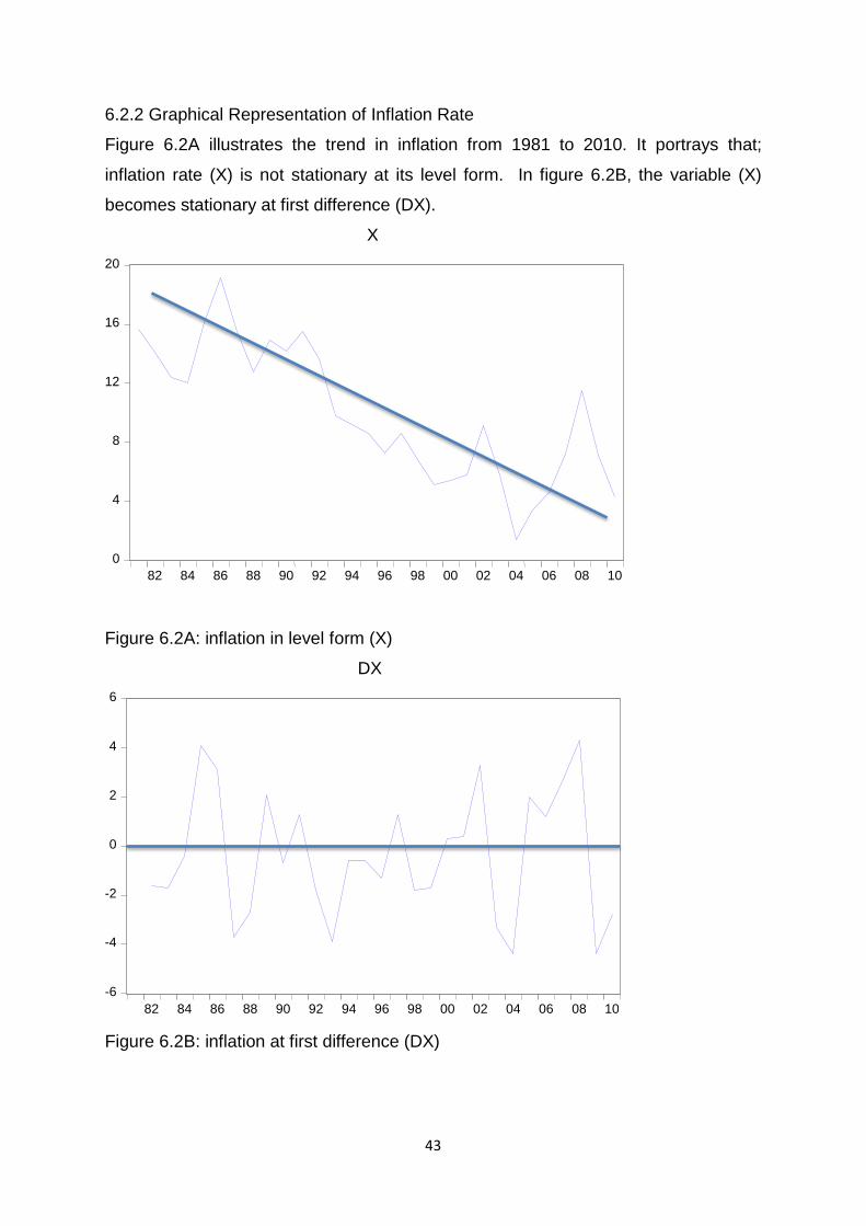
43
6.2.2 Graphical Representation of Inflation Rate
Figure 6.2A illustrates the trend in inflation from 1981 to 2010. It portrays that;
inflation rate (X) is not stationary at its level form. In figure 6.2B, the variable (X)
becomes stationary at first difference (DX).
Figure 6.2A: inflation in level form (X)
Figure 6.2B: inflation at first difference (DX)
0
4
8
12
16
20
82 84 86 88 90 92 94 96 98 00 02 04 06 08 10
X
-6
-4
-2
0
2
4
6
82 84 86 88 90 92 94 96 98 00 02 04 06 08 10
DX

44
6.2.3 Graphical Representation of Interest Rates
Figure 6.3A below illustrates the trend in real interest rates from 1981 to 2010. Real
interest rate appears to be non-stationary in its level form (R), but becomes
stationary when differenced once (DR) in figure 6.3B.
Figure 6.3A: Real interest rates in level form (R)
Figure 6.3B: Real interest rates at first difference (DR)
-4
0
4
8
12
16
82 84 86 88 90 92 94 96 98 00 02 04 06 08 10
R
-8
-4
0
4
8
12
82 84 86 88 90 92 94 96 98 00 02 04 06 08 10
DR

45
6.2.4 Graphical Representation of Unemployment Rate
Figure 6.4A: the unemployment rate (U) is not stationary in its level form, but
becomes stationary at first difference (DU) in figure 6.4B.
Figure 6.4A: Unemployment rate in level form (U)
Figure 6.4B: Unemployment rate at first difference (DU)
8
12
16
20
24
28
32
82 84 86 88 90 92 94 96 98 00 02 04 06 08 10
UT
-8
-6
-4
-2
0
2
4
6
82 84 86 88 90 92 94 96 98 00 02 04 06 08 10
DU

46
6.3 Unit Root Test Results
This section involves testing for the stationarity of the individual variables using both
the Augmented Dickey-Fuller and Phillips–Perron tests. Table 6.1 on the next page
(47) indicates the unit root test results performed in this study-following both the ADF
test and PP test. The Phillips-Perron test is used to verify the results obtained from
the ADF tests. Both tests are tested at a 1%, 5% and 10% level of significance and
are based on trend and intercepts, intercept and none. A maximum number of 3
lags were used for both the ADF and Phillips-Perron tests (as determined
automatically by E-views statistical package).
The dependent variable (Y) was found to be the stationary in its level form. This can
be seen by comparing the observed values of both the ADF test and PP test with the
critical values of the test statistics at all three levels of significance. Therefore, the
Null-Hypothesis is rejected and it is sufficient to conclude that there is no unit root in
the variable (Y) in its level form.
On the other hand, all independent variables are found be non-stationary in their
level forms. As a result, these variables were differenced once and both the ADF
test and PP test were performed on them as indicated in Table 6.1. Comparing the
observed values of both the ADF test and PP test with the critical values of the test
statistics revealed that all the independent variables were stationary at first
difference, and thus the Null-Hypothesis of non-stationarity is rejected followed by
the conclusion that all these variables are stationary.

47
Table 6.1: Results of units roots tests
Series Model ADF Phillips-Perron Test
Test
Lags tt tu t ϕ3 ϕ1 Lags tt tu t
tt 3 -4.419***
5.383 3 -4.849***
Yt tu 0 -4.030***
16.240***
3 -4.102***
T 0 -2.777***
- 3 -2.799***
tt 1 -3.489*
4.155 3 -2.628 Xt tu 1 -1.032 2.531 3 -1.414 T 1 -1.103 - 3 -1.465
tt 3 -8.573***
-34.124***
3 -7.299***
DXt tu 3 -8.397***
-41.377***
3 -7.465***
T 3 -8.640***
- 3 -7.648***
tt 0 -2.800 3.926 3 -2.816 Rt tu 0 -2.685*
7.208***
3 -2.682
T - - -1.183
tt 3 -8.573***
34.124***
3 -7.299***
DRt tu 3 -8.397***
41.377***
3 -7.465***
T 3 -8.640***
3 -7.648***
tt 0 -1.968 2.654 3 -1.952 Ut tu 0 -2.040 4.161**
3 -2.070
T - - - 3 0.880
tt 2 -6.175***
23.206***
3 -11.272***
DUt tu 2 -6.316***
32.329***
3 -11.472***
T 2 -6.439 - 3 -11.740***
Note : H0: Series contains a unit root : * [**] (***) indicate rejection of the null hypothesis at 10%, 5%, and
(1%) level of significance: : Yt; Rt; Xt; Ut indicate variables in level form : DXt; DRt; DUt; indicate variables at first difference : tt - Trend & Intercept; tu- Intercept; t- None : The ADF & PP tests were computed using Econometric E-Views
Package. Source: Author

48
6.4 The Long Run Relationship
Table 6.2 below presents the results of the long-run relationship between the
dependent variables and the independent variables. In this case, the variables are
used in their level forms and the model is tested for co-integration existence between
the dependent and independent variables. The model used in this study indicates
that a negative relationship is found between economic growth and the lagged
inflation rate.
TABLE 6.2: Results of long run relationship
Dependent Variable: Y Independent Variables Coefficient Xt-1 -0.589564
Rt-1 -0.101113 Ut -0.378553 C 12.19889
R-squared
0.686686
Adjusted R-squared 0.649088 S.E. of regression 1.406553 F-statistic 18.26405 D-W statistic 1.736202 Source: Author
6.5 Co-Integration Test Results: Augmented Engle-Granger Approach
Table 6.3 below indicates the unit root test performed on residuals. The test is
performed in order to determine the existence of co-integration between economic
growths (Y) and the independent variables (Xt, Ut and Rt). Comparing the
Mackinnon (1991) critical points and the ADF test statistic, it is decided to reject H0
at 10% level of significance. It is therefore concluded that there is co-integration
between the variables in the model, and thus, a long-run relationship does exist
between the variables.

49
Table 6.3: Co-integration test results
Variable
Model
Mackinnon (1991) Critical values
Lags
ADF t-statistic
0.01: C(1) = -5.288 0 -4.249* RESID01 None 0.05: C(5) = -4.4822 0 -4.249*
0.10: C(10) = -4.094 0 -4.249*
Note : Ho: No Co-integration; H1: Co-integration exists : * [**] (***) indicate rejection of the null hypothesis at 10%, 5%, and
1% level of significance: : The ADF test statistic was computed using Econometric E-Views
Package. Source: Author
6.6 Error Correction Model
Table 6.4 below presents the results on error correction model. The estimated
results indicate that the model is significant at 0.01 level of significance. Therefore, it
is sufficient to conclude that this model is of a good fit. Our findings denote that the
short-run effect of inflation targeting on economic growth is insignificant at all levels
of significance.
The error correction-term [RESIDOI (-1)] required magnitude of -0.844100 (which
indicates the speed of adjustment towards equilibrium) appears to be statistically
significance at 0.01. The estimated results also denote the R2 of 0.794050, which
means that about 79% change in the dependent variable (economic growth) are
explained by changes in the independent variables. In addition the coefficient of the
interaction dummy shows that the adoption of inflation targeting leads to a positive
effect of inflation on economic growth. However, such effect is not significant.

50
Table 6.4: Results of Error Correction-Model
Dependent variable (DYt)
Variable Coefficient
Std. Error t-Statistic P-Value Conclusion
DXt-1 -0.669684 0.165605 -4.043857 0.0006 Significant at 1
DUt -0.273310 0.132559 -2.061799 0.0518 Significant at 10% Dt -0.682766 0.562723 -1.213325 0.2385 Not significant
DRt-1 -0.483156 0.088153 -5.480886 0.0000 Significant at 1%
Dt*DXt-1 0.013754 0.221666 0.062048 0.9511 Not significant
RESID01-1 -0.844100 0.211500 -3.991019 0.0007 Significant at 1%
C 0.356233 0.365106 0.975698 0.3403 Not significant
R-squared 0.794050 Adjusted R-squared
0.735207
S.E. of regression 1.394197 F-statistic 13.49444 D-W statistic 2.133524 Source: Author
6.7 Diagnostic Tests
Table 6.5 presents the results of diagnostic tests which were carried out in order to
determine the quality of the model used. These results are tested based on the
levels of significance (L.O.S) 1%, 5% and 10%. According to Jargue-Bera test
performed in this study, the residuals of the regression are normally distributed in the
model because the p-value of 60% is greater than all the three levels of significance.
According to the Ljung-Box Q test of order (6), the model does not contain an
autocorrelation problem, because the P-value of 47% exceeds all three levels of
significance. The Breusch Godfrey test shows that there is no serial correlation in the
model, because the P-value is 11%, and greater than all the three levels of
significance.
Several other tests were performed in order to test for the heteroskedasticity problem
in the model, where first the Breusch-Pagan Godfrey test was performed and
revealed that the model is free from the heteroskedasticity problem, since the P-
value of 64% is greater than the three levels of significance. According to ARCH test
performed with a number of 2 lags, there is no problem of heteroskedasticity in the
model, because the P-value of 58% is greater than the three levels of significance.

51
In compliments to the ARCH results is the White test (with no cross terms (NCT) and
with cross terms (CT), which confirms that there is no heteroskedasticity in the
model, because the P-values of 74% for NCT and 48% for CT are greater than all
the three levels of significance.
In view of the diagnostic tests performed, it can be concluded that the model used in
this study is robust and as such reliable.
Table 6.5: Results from diagnostic tests
Test
H0 t-stat P-value Conclusion
Jarque-Bera
Residuals are normally distributed
1.017
0.602
Do not reject Ho since PV > L.O.S. Hence, residuals are normally distributed
Ljung-Box Q
No autocorrelation (order 6)
5.625
0.466
Do not reject Ho since PV > L.O.S. Hence, there is no autocorrelation in the model
Breusch-Godfrey
No-Serial correlation
4.371
0.1124
Do not reject Ho since PV > L.O.S. Hence, there is no serial correlation in the model
Breusch Pagan Godfrey
No Heteroskedasticity
4.282
0.639
Do not reject Ho since PV > L.O.S. Hence, there is no heteroskedasticity in the model
Arch
No-Arch Heteroskedasticity
0.303
0.582
Do not reject Ho since PV > L.O.S. Hence, there is no heteroskedasticity in the model
White (NCT)
No Heteroskedasticity
3.529
0.740
Do not reject Ho since PV > L.O.S. Hence, there is no heteroskedasticity in the model
White (CT)
No Heteroskedasticity
22.623
0.483
Do not reject Ho since PV > L.O.S. Hence, there is no heteroskedasticity in the model
Note : L.O.S means “level of significance” : PV means probability value : NCT means “no cross terms”; CT means with “cross terms”
6.8 Stability Tests
The stability test is performed using Ramsey Reset test in order to test for stability of
the model used. Table 6.6 below shows the results of stability test performed.
According to this test, the model is correctly specified because the P-value of 0.68 is
above all the three levels of significance. Therefore, it is insufficient evidence to
reject the null hypothesis (H0) and that the model is correctly specified.

52
Table 6.6: Results of stability test
Test H0 t-statistic P-value
Conclusion
Ramsey RESET
Equation is correctly specified
0.174036
0.6765
Do not reject H0 since PV > L.O.S. Hence, equation is correctly specified
6.9 Average Output and Output Variability
Table 6.7: Mean and variability
Period Mean Standard Deviation
Prior inflation targeting
2.1
2.4
After inflation targeting
3.7
2
Descriptive statistics were used to compare the mean and standard deviation of
economic growth between the period prior inflation targeting and after inflation
targeting. Table 6.7 shows that the average economic growth rate during inflation
targeting period is higher than the growth rate during the period prior to inflation
targeting by 1.6%. It also shows that growth variability has decreased by 0.4% after
the adoption of inflation targeting.
6.9 Conclusion
In this chapter, it has been possible to present and discuss the E-views estimated
results in both table and graphical forms. Annual time series data from 1981 to 2010
were used to estimate the coefficients of the error correction model used. The ADF
tests and the Phillips-Perron tests appear to be supporting the Error Correction
model used. For the purpose of reference, further tables showing complete results
of the analysis can be found in the appendixes on pages 60-71.

53
CHAPTER 7
CONCLUSION AND RECOMMENDATIONS
7.1 Introduction
The major conclusions are drawn and recommendations made on the basis of
literature reviewed in Chapter 2, research objectives and the research problem as
outlined in Chapter 1 and, most importantly, the hypotheses made in Chapter 1. In
this chapter, the format of the research report begins to widen again. It begins with a
review of conclusions drawn from a theoretical perspective followed by the
conclusions drawn from the findings of this study. It continues to outline its
limitations, followed by suggestions for future research. Lastly, possible
recommendations are given for the purpose of clarity and policy decision making in
South Africa.
7.2 Conclusions from the Theoretical Perspective
Stockton (1996) surveyed the existing literature related to price objectives for
monetary policy. In that survey Stockton identified several well-known established
empirical relationships pertinent to this topic. They included the following:
The evidence from both cross-country and time-series supports the notion that
Inflation reduces the growth of real output (or productivity).
In general relative price variability and inflation uncertainty adversely affect
real output.
In his recent book entitled Inflation Targeting (2003), Truman summarizes the
principal conclusions of the empirical literature on inflation targeting. In particular,
inflation targeting has had favourable effects on inflation, inflation variability,
inflation expectations and the persistence of inflation. But it has not had a
negative effect on economic growth, the variability of growth, or
unemployment.

54
7.3 Conclusions from Findings in the present study
After a decade of adopting inflation targeting by the SARB as its monetary policy
framework, debates have erupted among politicians, economists, labour unions etc.,
about the effects of this policy on economic growth in South Africa. The main
purpose of this study was to determine the effects of inflation targeting on economic
growth in South Africa. In order to achieve this purpose a comprehensive literature
review was carried out to review what other authors found when making similar
studies. An Error Correction model was used to achieve the following research
objectives:
To establish how inflation targeting affected economic growth;
To determining whether inflation targeting reduced or promoted economic
growth in South Africa;
To determining whether inflation targeting led to high or low variations in the
level of economic growth;
To identify the challenges facing inflation targeting monetary policy framework
objective to ensure stable inflation, while maintaining high and stable long
term economic growth in South Africa; and
To establish whether inflation targeting has been conducive to high and stable
long term economic growth in South Africa as a semi-developed country.
These objectives have been achieved as discussed in the last four chapters. Most
importantly, an error correction model was used to estimate the short-run effects of
inflation targeting on economic growth and the long run effects were estimated using
a multiple regression model. The error correction model used was tested for
robustness using diagnostic tests which showed that the model is robust and
therefore reliable. In addition to the diagnostic tests a stability test showed that the
model is correctly specified. The following decision rule on the hypotheses and
conclusions were drawn from the findings of this study:
HYPOTHESES
H0: the Inflation targeting monetary policy as employed in South Africa does
not significantly influence economic growth.

55
H1: Inflation targeting monetary policy as employed in South Africa does
significantly influence economic growth.
Decision: Do not reject the null hypothesis at 0.1 level of significance; implying that
there is no adequate evidence to reject the null hypothesis.
Based on descriptive statistics a preliminary conclusion could be drawn from the
evidence below that inflation targeting has positive effects on economic growth.
The average economic growth rate was compared between the period before
inflation targeting and after inflation targeting. It was found that average
economic growth rates remained low and, in many instances, remained
negative during the period prior to inflation targeting. However, the average
economic growth rate has consistently remained steady and relatively high
during the inflation targeting period.
The period prior to inflation targeting shows that there was high output
variability as compared to output variability for the period during inflation
targeting. This leads to the conclusion that inflation targeting does not only
reduce variability in inflation but also in economic growth, though, it is hard to
prove whether this reduced variability can be attributed to inflation targeting
alone or due to other-external-factors that may have played a role.
Based on the following important findings (obtained by using Error Correction Model
which is tested for robustness and reliability) a final conclusion is drawn that inflation
targeting monetary policy, as employed in South Africa, does not have significant
negative effects on economic growth.
There is a negative relationship between inflation targeting and economic
growth in South Africa. However, this negative relationship between inflation
targeting and economic growth was found to be statistically insignificant.
The influence that inflation targeting has on the relationship between the lag
of inflation and economic growth is also statistically insignificant.

56
7.4 Limitations of the Study
It should be noted that it is not possible to cover all the aspects of a particular field of
enquiry in a single study. In this section, the aspects of research that were not
covered are highlighted and these will identity priorities for future research.
This study focuses on the effects of inflation targeting on economic growth in
South Africa. This means that it is limited to a South African context; and
therefore, is not applicable to any other region outside South Africa.
The comparison between economic growth before the inflation targeting
period and after inflation targeting may lead to bias. The period before
inflation targeting was characterized by several changes in the monetary
policy regime, such as the monetary aggregate target and exchange rate
targeting.
This study used annual time series data from 1981 to 2010 to compare the
period prior and after inflation targeting. The data were not enough because
inflation targeting was only adopted in the year 2000.
Considering the fact that the inflation targeting policy framework was adopted
in 2000 in South Africa, there is a limited research conducted on similar
subjects like this one.
7.5 Future Research
The results found here were based on annual time series data from 1981 to
2010. This means that the impact of inflation targeting on economic growth in
South Africa should be monitored and compared with the findings in this study
and beyond the year 2010.
The present research focuses on a few casual variables and there may still be
a need to study other relevant variables to determine whether they give the
same findings as the ones found in this study.
This study narrowed its focus to a South African context. This means a
similar approach can be used to study other countries cases.
This study used the error correction model to estimate the relationship
between inflation targeting and economic growth. Therefore, it invites the
researcher to criticize this model and prove its relevancy.

57
7.6 Recommendations
The possible impact of inflation targeting on economic growth is a concern in South
Africa and continues to receive a lot of attention in monetary economics literature.
Based on the findings of this study the following recommendations can be made:
It is generally accepted that instability in the general level of prices causes
substantial economic distortions, leading to inefficiencies, both in aggregate
employment and output. It is also evident that the effects of inflation targeting
on economic growth in South Africa are relatively insignificant. There is no
evidence that inflation targeting promotes or reduces economic growth in SA.
The critique that the SARB achieves low inflation at the expense of low
economic growth is probably a misconception. Therefore, the SARB should
maintain its monetary policy framework which has helped it to reduce inflation
and most importantly inflation expectations.
It has also been realized that certain SARB stakeholders (COSATU and
SACP) often criticize the decisions of the Monetary Policy Committee (MPC)
without adequate information. For the purpose of clarity these stakeholders
need to be invited to monetary policy seminars that are regularly held by the
SARB MPC. This will ease the difficulty these institutions have to better
understand certain decisions taken by the SARB.
It is important for different SARB stakeholders to note that the SARB long
term primary objective is to ensure price stability. It is not primarily responsible
for achieving economic growth. Therefore, critique of inflation targeting
impact on economic growth should bear in mind this objective as stated
clearly in the SA Act 108 of 1996.
Last but not least, a successful inflation targeting policy will require the support of
labour unions, businesses, the private sector and the government sector to show
confidence in the monetary policy of the SARB.
58
REFERENCES
Ammer, J., & Freeman, R.T. 1995. “Inflation targeting in the 1990s: The experience
of New Zealand, Canada, and the United Kingdom”. Journal of Economics and
Business, 47, 165-192.
Arnold, R. 2008. Economics, 8th Edition. California: Thomson South-Western
Corporation.
Asteriou, D. and Hall, S.G. 2011. Applied Econometrics. Palgrave Macmillan. 234.
Babbie, E. 1992. The Practice of Social Research. Belmont, California: Wadsworth
Bailey, K. 1987. Methods of Social Research. New York: Collier Macmillan.
Ball, L. 1997. Efficient Rules for Monetary Policy. NBER Working Paper No: 5952.
Barro, R. 1991. Economic growth in a cross section of countries. Quarterly Journal of
Economics, Vol 106, 407 – 443.
Barro, R.J. 1995. Determinants of Economic Growth. New York: McGraw-Hill.
Barro, R. 2001. Economic growth in East Asia before and after the financial crisis.
NBER Working Paper 8330. 4, June.
Batini, N., & Laxton, D. 2006. Under what conditions can inflation targeting be
adopted? The experience of emerging markets. Working Paper 406. Central
Bank of Chile.
Begg, D., Fischer, S., & Dornbusch, R. 2005. Economics, 8th Edition. McGraw-Hill
Education. Madrid.
Bernanke, B. 2003. A perspective of inflation targeting. Journal of Business
Economics. Volume 38, 7 – 15.
Bernanke, B., & Mishkin, F. 1997. Inflation Targeting: A New Framework for
Monetary Policy? Journal of Economic Perspectives. Vol 11, 97-116.
Bhar, R. 2010. Statistical Mechanics and its Applications Journal. Vol 389: 1
December, 5503 – 5510.
Blanchard, O. 2006. Macroeconomics. Upper Saddle River. New Jersey: Pearson
Prentice Hall.
Brimmer, F. 2002. Inflation targeting in Chile. The North American Journal of
Economics and Finance. Vol 13: 2 August, 93 – 97.
Brito, D., & Bystedt, B. 2010. Inflation targeting in emerging markets: Panel
evidence. Journal of Development Economics. Vol 91: 2 March, 198 – 210.
Cecchetti, S., and M. Ehrmann. 2000. Does inflation targeting increase output

59
volatility? An international comparison of policymakers’ preferences and
outcomes. Central Bank of Chile Working Papers no, 69.
Chari, V., Jones, L., & Manuelli, R. 1996. Inflation, growth, and financial
intermediation Journal. Federal Reserve Bank of st. Louis, May, 41 – 58.
Chetty, S., Greyling, L., van Zyl, G., Schoeman, C., Wentzel, A. 2010. A Basic
Approach to Fundamental Economic Theory. Third Edition. APT print and
paper solution. Johannesburg.
Civcir, I, and Akcaglayan, A. 2010. Inflation targeting and the exchange rate: Does it
matter in Turky? Journal of Policy Modeling. Vol 32, 339 – 354.
Corbo, V., Landerretche, O., and Schmidt-Hebbel, K. 2002. Does Inflation Targeting
Make a Difference? in Inflation Targeting: Design, Performance, Challenges.
Vol 5. Santiago: Bank of Chile. pp. 221-69.
COSATU. 2007. Statement on interest rates. Mail and Guardian. 10 September.
Debelle, G. 1995. Monetary Policy Goals for Inflation in Australia, Targeting Inflation.
London: Bank of England.
Domar E.D. 1966. Essays in the Theory of Economic Growth. New York, NY, USA.
pp 272.
Dornbusch, R., Fischer S., & Kearney C. 1996. Macroeconomics. Sydney: The Mc-
Graw-Hill Companies, Inc.
Du Plessis, S.A., and Smit B.W. 2006. Economic growth in South Africa since 1994.
Bureau of Economic Research, Stellenbosch Economic working paper:1
Epstein, G.A. & Erinc Yeldan, A. 2009. Beyond inflation targeting, Assessing the
impacts and policy alternatives. Edward Elgar Publishing Limited. UK,
Cheltenham.
Fischer, S. 1993. The Role of Macroeconomics Factors in Growth. Journal of
Monetary Economics. Vol 32. M.I.T Cambridge, USA.
Friedman, M. and Schwatz, A.J. 1963. A Monetary History of the United States 1867
– 1960. Princeton: Princeton University Press.
Gay, L. R. 1987. Educational Research: Competencies for Analysis and Application.
3rd Edition. Columbus, Merrill Publishing Company. pp 101.
Ghatak, S., and Sanchez-Fung, J.R. 2007. Monetary Economics in Developing
Countries. 3rd Edition. PALGRAVE MACMILLAN, New York.
Gillepie, A. 2011. Foundation of Economics. 2nd Edition. New York: Oxford
University.

60
Gokal, V. 2004. Relationship between Inflation and Economic Growth. Reserve Bank
of Fiji. Working Paper2004/04.
Gordhan, P. 2009. Public address. Sowetan Newspaper, South Africa.
Gregorio, J. 1992. Economic growth in Latin American. Journal of Development
Economics. Vol 39, 59 – 84.
Gujarati, D.N. 1998. Essentials of Econometrics. McGraw Hill, Boston. Page 534
Gujarati, D.N. (2006). Essentials of Econometrics. 3rd Edition. U.S. Military
Academy, West Point: McGraw-Hill Higher Education.
Gujarati, D.N., and Porter, D. 2009. Essentials of Econometrics. 4th Edition.
McGraw-Hill Education.
Gylfason, T., & Herbertsson, T. 2001. Does inflation matter for growth? Japan and
the World Economy Journal. Vol 13, 405 – 428.
Halcoussis, D. 2005. Understanding Econometrics. Thomson Corporation, USA. pp
7.
Handa, J. 2000. Monetary Economics. London: Routledge 11 New Fetter publisher,
Harrod R.F. 1939. An essay in dynamic economics. Economic Journal. Vol 49, pp
14-33.
Haslag, J. H. 1995. Output, Growth, Welfare and Inflation: A Survey. Economic
Review Second Quarter, Federal Reserve Bank of Dallas.
International Monetary Funds. 2006. Inflation targeting and the IMF. IMF,
Washington, March.
Johnson, D. 2002. “The effect of inflation targeting on the behavior of expected
inflation: Evidence from an 11 country panel”, Journal of Monetary Economics,
Vol 49, 1521-1538.
Judge, G.G, Griffiths, W.E., and Hill, R.C. 2011. The Theory and practices of
Econometrics, 2nd Ed. (New York: John Wiley).
Kakwani, N. 2008. Global estimates of pro-poor growth. Journal of World Development. Vol 36, 1048 – 1066.
Kormendi, R., & Meguire, P. 1985. Macroeconomic determinants of growth: Cross country evidence. Journal of Monetary Economics, Vol 16, 141 – 163.
Kuttner K.N. 2004. The role of policy rules in inflation targeting. Federal Reserve Bank of St. Louis Review, 86(4). pp 89–111. Kuttner, K.N., Friedman, M., and Benjamin M. 1996. A Price Target for U.S.
Monetary Policy? Lessons from the Experience with Money Growth Targets.
Brookings Papers on Economic Activity. Vol 1. pp 77–146.

61
Laubscher, J. 2013. Economic growth in South Africa: a 20-year review. South
Africa, December.
MacKinnon, J. G. 1991, “Critical values for cointegration tests,”Long-Run Economic
Relationships: Readings in Cointegration. Oxford, Oxford University Press.
McConnell, C.R., and Brue, S.L. 2005. Economics: Principles, problems and policies.
McCRAW-HILL, New York.
Mboweni, T.T. 2006. 'Statement of the Monetary Policy Committee', 03 August
2006, Pretoria, South Africa, pp. 1-4.
Meyer, L.H. 2002. Inflation targets and inflation targeting. North American Journal of
Economics and Finance, Vol 13. pp 147-162.
Mignon, V. 2011. On the impact of inflation on output growth: Does the level of
inflation matter? Journal of Macroeconomics. Vol 33. pp 455–464
Mishkin, F.S. 1999. Inflation targeting in emerging markets countries. Cambridge.
National Bureau of Economic Research. London: Daryl Fox publisher.
Mishkin, F.S. 1999. “International experiences with different monetary policy
regimes”, Journal of Monetary Economics, Vol 43, 579-605.
Mishkin, F.S. 2000. Inflation targeting in emerging market countries. National Bureau
of Economic Research. Working Paper 7618. pp 1-12
Mishkin, F.S. 2006. The Economics of Money, Banking and Financial Markets,
seventh edition. London: Daryl Fox publisher.
Mishkin, F.S., & Schmidt-Hebbel, K. 2007. Monetary Policy under inflation targeting.
Central Bank of Chile, Santiago, 1- 38.
Mishkin, F.S. 2010. The economics of money, banking and financial markets. Global
edition, Pearson.
Mohr, P., Fourie, L., & Associates. 2008. Economics for South African Students, 4th
edition. Van Schaik publishers, Pretoria.
Mollick, A., Cabral, R., & Garneiro, G. 2011. Does inflation targeting matter for output
growth? Evidence from industrial and emerging economies. Journal of Policy
Modeling. Vol 33: 4 July, 537 – 551.
Noula, AG. 2012. Fiscal deficit and nominal interest rate determination in Cameroon:
An application of the loan able funds model. Global Advanced Research
Journal of Management and Business Studies. Vol 1: 006-029.
Pentecost, E. 2000. Macroeconomics: an open economy approach, New York: St
Mratins Press.

62
Petursson, G. 2004. The effects of inflation targeting on macroeconomic
performance. National Bureau of Economic Research, Working Paper 23, 7.
Pereira, G.L. 2009. Australian Critical Care, Volume 22. 4, November, Pages 187-
191
Pollin, R., and Zhu, A. 2006. Inflation and Economic Growth: A Cross-Country
Nonlinear Analysis. Journal of Post Keynesian Economics. Summer. Vol. 28,
pp. 593-614.
Polit, DF & Hungler, BP. 1999. Nursing research: Principles and methods. 6th
edition. Philadelphia: Lippincott.
Robson, C. 1993. Real World Research. Oxford: Blackwell. pp 283-9
Romer, P. M. 1986. “Increasing Returns and Long Run Growth.” The Journal of
Political Economy, vol 94.
SARB 2006, 'Monetary Policy Review', May 2006, pp. 1-33.
Sarel, M. 1996. Nonlinear effect of inflation on economic growth. International
Monetary Fund. Journal of Monetary Economics, Vol 43, 199 – 215
Stockton, D.J. 1996. The Price Objective for Monetary Policy: An Outline of the
Issues. A Report to the FOMC Board of Governors. 20, June.
Sheridan, N., & Ball, L. 2005. Does inflation targeting matter? (Working paper NO:
9577). Massachusetts Avenue Cambridge, MA 02138.
Solow, R.M. 1956. “A contribution to the Theory of Economic Growth.” Quarterly
Journal of Economics, vol 70.
Studenmund, A.H. 2006. Using Econometrics. Fifth Edition. Daryl Fox. USA. pp 6.
Svensson, L. 2007. Inflation targeting. The new Palgrave dictionary of economics.
Second edition. Working Paper 3, March.
Svensson, EO. 2010. Inflation targeting. National Bureau of Economic Research.
Working Paper: 16654, December. 1050 Massachusetts Avenue Cambridge.
Swan, T. W. 1956. “Economic Growth and Capital Accumulation”. Economic Record,
32. Pp 334-61
Truman, E. 2003. Inflation targeting in the world economy. Institute for International
Economics.
Van den Heever, JP. 2001. A note on inflation targeting in South Africa. The South
African Journal of Economics, Vol 69:1, March
Van Der Merwe, EJ. 2004. Inflation targeting in South Africa. Occasional paper NO:
19, JULY.

63
Van Der Merwe, M. 2010. Monetary economics. Oxford University Press Southern
Africa, Cape Town, South Africa.
Webster, J.T. 1984. A comparison of some approximate F test. Technometrics, 15.
pp 779-789
Wray, R., & Forstater, M. 2006. Money, Financial instability and Stabilization policy.
Published by Edward Elgar LTD, UK: Cheltenham.

64
APPENDICES Appendix A: Long Run Equilibrium Equation Dependent Variable: Y Method: Least Squares Date: 12/11/13 Time: 17:09 Sample (adjusted): 1982 2010 Included observations: 29 after adjustments Variable Coefficient Std. Error t-Statistic Prob. Xt-1 -0.589564 0.094299 -6.252086 0.0000 Ut -0.101113 0.076311 -1.324998 0.1972
Rt-1 -0.378553 0.086694 -4.366566 0.0002 C 12.19889 2.510014 4.860089 0.0001 R-squared 0.686686 Mean dependent var 2.200000 Adjusted R-squared 0.649088 S.D. dependent var 2.374417 S.E. of regression 1.406553 Akaike info criterion 3.647603 Sum squared resid 49.45976 Schwarz criterion 3.836195 Log likelihood -48.89024 Hannan-Quinn criter. 3.706667 F-statistic 18.26405 Durbin-Watson stat 1.736202 Prob(F-statistic) 0.000002

65
Appendix B: Error Correction Model (ECM) Dependent Variable: DY Method: Least Squares Date: 12/11/13 Time: 17:27 Sample (adjusted): 1983 2010 Included observations: 28 after adjustments Variable Coefficient Std. Error t-Statistic Prob. DXT(-1) -0.669684 0.165605 -4.043857 0.0006 DRT(-1) -0.483156 0.088153 -5.480886 0.0000 DUT -0.273310 0.132559 -2.061799 0.0518 DT -0.682766 0.562723 -1.213325 0.2385 DT*DXT(-1) 0.013754 0.221666 0.062048 0.9511 RESID01(-1) -0.844100 0.211500 -3.991019 0.0007 C 0.356233 0.365106 0.975698 0.3403 R-squared 0.794050 Mean dependent var 0.117857 Adjusted R-squared 0.735207 S.D. dependent var 2.709387 S.E. of regression 1.394197 Akaike info criterion 3.714832 Sum squared resid 40.81946 Schwarz criterion 4.047883 Log likelihood -45.00764 Hannan-Quinn criter. 3.816649 F-statistic 13.49444 Durbin-Watson stat 2.133524 Prob(F-statistic) 0.000003

66
DIAGNOSTIC TESTS ON ECM Appendix C: Autocorrelation Date: 12/12/13 Time: 06:07 Sample: 1983 2010 Included observations: 28 Autocorrelation Partial Correlation AC PAC Q-Stat Prob . *| . | . *| . | 1 -0.154 -0.154 0.7346 0.391 . | . | . | . | 2 0.056 0.033 0.8364 0.658 . | . | . | . | 3 0.012 0.026 0.8414 0.840 . |* . | . |* . | 4 0.133 0.140 1.4564 0.834 .**| . | .**| . | 5 -0.336 -0.311 5.5855 0.349 . | . | . *| . | 6 0.032 -0.075 5.6252 0.466

67
Appendix D: Normality Tests on Residuals
0
1
2
3
4
5
6
-3.0 -2.5 -2.0 -1.5 -1.0 -0.5 0.0 0.5 1.0 1.5 2.0 2.5
Series: Residuals
Sample 1983 2010
Observations 28
Mean 1.63e-16
Median 0.219484
Maximum 2.003010
Minimum -2.597492
Std. Dev. 1.229566
Skewness -0.264878
Kurtosis 2.231415
Jarque-Bera 1.016591
Probability 0.601520

68
Appendix E: Serial Correlation Breusch-Godfrey Serial Correlation LM Test: F-statistic 1.757503 Prob. F(2,19) 0.1994 Obs*R-squared 4.371314 Prob. Chi-Square(2) 0.1124 Test Equation: Dependent Variable: RESID Method: Least Squares Date: 12/12/13 Time: 06:12 Sample: 1983 2010 Included observations: 28 Presample missing value lagged residuals set to zero. Variable Coefficient Std. Error t-Statistic Prob. DXT(-1) 0.021294 0.163336 0.130370 0.8976 DRT(-1) -0.015550 0.086438 -0.179899 0.8591 DUT 0.013535 0.128439 0.105383 0.9172 DT 0.321599 0.577911 0.556485 0.5844 DT*DXT(-1) -0.029565 0.221556 -0.133441 0.8952 RESID01(-1) 0.879471 0.515820 1.704995 0.1045 C -0.130217 0.359618 -0.362099 0.7213 RESID(-1) -1.047577 0.565889 -1.851206 0.0797 RESID(-2) -0.086403 0.249392 -0.346457 0.7328 R-squared 0.156118 Mean dependent var 1.63E-16 Adjusted R-squared -0.199200 S.D. dependent var 1.229566 S.E. of regression 1.346473 Akaike info criterion 3.687946 Sum squared resid 34.44680 Schwarz criterion 4.116154 Log likelihood -42.63124 Hannan-Quinn criter. 3.818853 F-statistic 0.439376 Durbin-Watson stat 1.725065 Prob(F-statistic) 0.882483

69
Appendix F: Heteroskedasticity Heteroskedasticity Test: Breusch-Pagan-Godfrey F-statistic 0.631833 Prob. F(6,21) 0.7033 Obs*R-squared 4.281712 Prob. Chi-Square(6) 0.6386 Scaled explained SS 1.482909 Prob. Chi-Square(6) 0.9606 Test Equation: Dependent Variable: RESID^2 Method: Least Squares Date: 12/12/13 Time: 06:14 Sample: 1983 2010 Included observations: 28 Variable Coefficient Std. Error t-Statistic Prob. C 1.310929 0.450234 2.911661 0.0083 DXT(-1) -0.130374 0.204218 -0.638404 0.5301 DRT(-1) -0.037776 0.108707 -0.347504 0.7317 DUT 0.053348 0.163467 0.326355 0.7474 DT 0.199286 0.693928 0.287185 0.7768 DT*DXT(-1) -0.153094 0.273350 -0.560066 0.5814 RESID01(-1) 0.104404 0.260813 0.400301 0.6930 R-squared 0.152918 Mean dependent var 1.457838 Adjusted R-squared -0.089105 S.D. dependent var 1.647437 S.E. of regression 1.719268 Akaike info criterion 4.133992 Sum squared resid 62.07353 Schwarz criterion 4.467043 Log likelihood -50.87589 Hannan-Quinn criter. 4.235809 F-statistic 0.631833 Durbin-Watson stat 1.506802 Prob(F-statistic) 0.703342

70
Appendix G: Heteroskedasticity Heteroskedasticity Test: ARCH F-statistic 0.283335 Prob. F(1,25) 0.5992 Obs*R-squared 0.302572 Prob. Chi-Square(1) 0.5823 Test Equation: Dependent Variable: RESID^2 Method: Least Squares Date: 12/12/13 Time: 06:16 Sample (adjusted): 1984 2010 Included observations: 27 after adjustments Variable Coefficient Std. Error t-Statistic Prob. C 1.137520 0.345670 3.290766 0.0030 RESID^2(-1) 0.083007 0.155942 0.532292 0.5992 R-squared 0.011206 Mean dependent var 1.261944 Adjusted R-squared -0.028345 S.D. dependent var 1.304847 S.E. of regression 1.323211 Akaike info criterion 3.469187 Sum squared resid 43.77220 Schwarz criterion 3.565175 Log likelihood -44.83403 Hannan-Quinn criter. 3.497730 F-statistic 0.283335 Durbin-Watson stat 1.863122 Prob(F-statistic) 0.599223

71
Appendix H: Heteroskedasticity Heteroskedasticity Test: White F-statistic 0.504725 Prob. F(6,21) 0.7978 Obs*R-squared 3.528903 Prob. Chi-Square(6) 0.7401 Scaled explained SS 1.222185 Prob. Chi-Square(6) 0.9758 Test Equation: Dependent Variable: RESID^2 Method: Least Squares Date: 12/12/13 Time: 06:17 Sample: 1983 2010 Included observations: 28 Variable Coefficient Std. Error t-Statistic Prob. C 2.106953 0.824142 2.556541 0.0184 DXT(-1)^2 -0.071785 0.085015 -0.844386 0.4080 DRT(-1)^2 -0.005168 0.017930 -0.288207 0.7760 DUT^2 -0.024004 0.047654 -0.503702 0.6197 DT^2 -1.134780 1.011791 -1.121556 0.2747 (DT*DXT(-1))^2 0.170687 0.108735 1.569756 0.1314 RESID01(-1)^2 -0.087738 0.184368 -0.475887 0.6391 R-squared 0.126032 Mean dependent var 1.457838 Adjusted R-squared -0.123673 S.D. dependent var 1.647437 S.E. of regression 1.746339 Akaike info criterion 4.165239 Sum squared resid 64.04372 Schwarz criterion 4.498290 Log likelihood -51.31334 Hannan-Quinn criter. 4.267056 F-statistic 0.504725 Durbin-Watson stat 1.307144 Prob(F-statistic) 0.797785

72
Appendix I: Heteroskedasticity Heteroskedasticity Test: White F-statistic 0.731772 Prob. F(23,4) 0.7237 Obs*R-squared 22.62334 Prob. Chi-Square(23) 0.4829 Scaled explained SS 7.835266 Prob. Chi-Square(23) 0.9986 Test Equation: Dependent Variable: RESID^2 Method: Least Squares Date: 12/12/13 Time: 06:18 Sample: 1983 2010 Included observations: 28 Collinear test regressors dropped from specification Variable Coefficient Std. Error t-Statistic Prob. C 0.417504 2.488167 0.167796 0.8749 DXT(-1) -0.005361 0.673886 -0.007955 0.9940 DXT(-1)^2 -0.186375 0.315613 -0.590515 0.5866 DXT(-1)*DRT(-1) -0.085708 0.133621 -0.641424 0.5562 DXT(-1)*DUT -0.585247 0.401257 -1.458532 0.2184 DXT(-1)*DT 0.726800 0.921712 0.788533 0.4745 DXT(-1)*(DT*DXT(-1)) 0.099689 0.391631 0.254548 0.8116 DXT(-1)*RESID01(-1) -0.171734 0.593438 -0.289388 0.7867 DRT(-1) 1.149128 1.090800 1.053472 0.3516 DRT(-1)^2 0.094712 0.086029 1.100931 0.3327 DRT(-1)*DUT -1.404810 0.904118 -1.553791 0.1952 DRT(-1)*DT 1.305015 1.644248 0.793685 0.4718 DRT(-1)*(DT*DXT(-1)) 0.987933 0.728865 1.355441 0.2468 DRT(-1)*RESID01(-1) 0.139757 0.291041 0.480196 0.6562 DUT 3.094611 1.845106 1.677199 0.1688 DUT^2 -0.194367 0.189084 -1.027939 0.3621 DUT*DT -3.350076 2.387857 -1.402963 0.2333 DUT*(DT*DXT(-1)) -0.459688 0.719104 -0.639251 0.5574 DUT*RESID01(-1) -1.446379 0.939580 -1.539390 0.1985 DT 0.670967 2.765903 0.242585 0.8203 DT*RESID01(-1) -1.406037 1.937360 -0.725749 0.5082 (DT*DXT(-1))*RESID01(-1) 0.108628 0.818919 0.132648 0.9009 RESID01(-1) 1.874701 1.619532 1.157557 0.3115 RESID01(-1)^2 -1.014135 0.668474 -1.517090 0.2038 R-squared 0.807976 Mean dependent var 1.457838 Adjusted R-squared -0.296160 S.D. dependent var 1.647437 S.E. of regression 1.875591 Akaike info criterion 3.864100 Sum squared resid 14.07136 Schwarz criterion 5.005989 Log likelihood -30.09740 Hannan-Quinn criter. 4.213187 F-statistic 0.731772 Durbin-Watson stat 2.250085 Prob(F-statistic) 0.723716

73
MISSPECIFICATION Appendix J: Stability Test Ramsey RESET Test Equation: ECM Specification: DY DXT(-1) DRT(-1) DUT DT DT*DXT(-1) RESID01(-1) C Omitted Variables: Squares of fitted values Value Df Probability
t-statistic 0.353126 20 0.7277 F-statistic 0.124698 (1, 20) 0.7277 Likelihood ratio 0.174036 1 0.6765 F-test summary:
Sum of Sq. df Mean Squares
Test SSR 0.252929 1 0.252929 Restricted SSR 40.81946 21 1.943784 Unrestricted SSR 40.56653 20 2.028327 Unrestricted SSR 40.56653 20 2.028327 LR test summary: Value df
Restricted LogL -45.00764 21 Unrestricted LogL -44.92062 20 Unrestricted Test Equation: Dependent Variable: DY Method: Least Squares Date: 12/12/13 Time: 06:22 Sample: 1983 2010 Included observations: 28 Variable Coefficient Std. Error t-Statistic Prob. DXT(-1) -0.677479 0.170602 -3.971098 0.0008 DRT(-1) -0.474708 0.093173 -5.094900 0.0001 DUT -0.258727 0.141568 -1.827577 0.0826 DT -0.675998 0.575150 -1.175342 0.2537 DT*DXT(-1) 0.010813 0.226589 0.047722 0.9624 RESID01(-1) -0.871834 0.229882 -3.792522 0.0011 C 0.410160 0.403016 1.017728 0.3210 FITTED^2 -0.011603 0.032858 -0.353126 0.7277 R-squared 0.795326 Mean dependent var 0.117857 Adjusted R-squared 0.723691 S.D. dependent var 2.709387 S.E. of regression 1.424193 Akaike info criterion 3.780045 Sum squared resid 40.56653 Schwarz criterion 4.160674 Log likelihood -44.92062 Hannan-Quinn criter. 3.896407 F-statistic 11.10236 Durbin-Watson stat 2.103852 Prob(F-statistic) 0.000011

74
Appendix K: Data (1981-2010)
obs Y XT UT RT DT
1981 5.4 15.7 9.8 3.7 0
1982 -0.4 14.1 10.8 4.7 0
1983 -1.8 12.4 12.5 0.1 0
1984 5.1 12 13.7 9.7 0
1985 -1.2 16.1 15.5 4 0
1986 0 19.2 16.1 -2.3 0
1987 2.1 15.5 16.6 -1.8 0
1988 4.2 12.8 17.2 0.13 0
1989 2.4 14.9 17.8 2.2 0
1990 -0.3 14.2 18.8 4.7 0
1991 -1 15.5 20.2 4 0
1992 -2.1 13.7 21.2 3.8 0
1993 1.2 9.8 22.2 2.7 0
1994 3.2 9.2 22.9 5.5 0
1995 3.1 8.6 16.7 6.9 0
1996 4.3 7.3 19.3 10.6 0
1997 2.6 8.6 21 11 0
1998 0.5 6.8 25.2 13.1 0
1999 2.4 5.1 23.4 10.2 0
2000 4.2 5.4 25.6 5.2 1
2001 2.7 5.8 29.4 5.7 1
2002 3.7 9.1 30.4 4.5 1
2003 2.9 5.8 28 8.9 1
2004 4.6 1.4 26.2 4.6 1
2005 5.3 3.4 26.7 4.9 1
2006 5.6 4.6 25.5 4.4 1
2007 5.5 7.2 22.2 4.6 1
2008 3.6 11.5 22.9 5.4 1
2009 -1.5 7.1 23.9 4.1 1
2010 2.9 4.3 24.9 5.3 1

75
Appendix L: Descriptive Statistics 1981-1999 2000-2010
Y
Mean 3.590909
Median 3.7
Maximum 5.6
Minimum -1.5
Std. Dev. 1.99171
Skewness -1.48668
Kurtosis 4.977552
Jarque-Bera 5.844466
Probability 0.053813
Sum 39.5
Sum Sq. Dev. 39.66909
Observations 11
Y
Mean 1.563158
Median 2.1
Maximum 5.4
Minimum -2.1
Std. Dev. 2.350463
Skewness 0.02542
Kurtosis 1.798807
Jarque-Bera 1.144313
Probability 0.564307
Sum 29.7
Sum Sq. Dev. 99.44421
Observations 19