Abstract This paper describes a series of four pro-grammes for the PC based on ellipsoidal representationsof macromolecular shape in solution using Universal shapefunctions. ELLIPS1 is based on simple ellipsoid of revo-lution models (where two of the three axes of the ellipsoidare fixed equal to each other). If the user types in a valuefor a shape function from sedimentation or other types ofhydrodynamic measurement, it will return a value for theaxial ratio of the ellipsoid. ELLIPS2 is based on the moregeneral triaxial ellipsoid with the removal of the restric-tion of two equal axes. The user enters the three semi-axialdimensions of the molecule or the equivalent two axial ra-tios and ELLIPS2 returns the value of all the hydrodynamicshape functions. It also works of course for ellipsoids of revolution. ELLIPS3 and ELLIPS4 do the reverse of ELLIPS2, that is they both provide a method for the uniqueevaluation of the triaxial dimensions or axial ratios of amacromolecule (and without having to guess a value forthe so-called “hydration”) after entering at least threepieces of hydrodynamic information: ELLIPS3 requiresEITHER the intrinsic viscosity with the second virial co-efficient (from sedimentation equilibrium, light scatteringor osmometry) and the radius of gyration (from light or x-ray scattering) OR the intrinsic viscosity with the con-centration dependence term for the sedimentation coeffi-cient and the (harmonic mean) rotational relaxation timefrom fluorescence depolarisation measurements. ELLIPS4evaluates the tri-axial shape of a macromolecule fromelectro-optic decay based Universal shape functions usinganother Universal shape function as a constraint in the ex-traction of the decay constants.

Key words Macromolecular shape · Ellipsoids ·Hydrodynamics

Introduction

There are two approaches to representing the conforma-tion of fairly rigid macromolecules in solution. The firstapproach is the so-called “Bead” or “Multiple sphere” ap-proach pioneered by V. A. Bloomfield at the University ofMinnesota and J. Garcia de la Torre at the University ofMurcia (see, e.g. Garcia de la Torre and Bloomfield 1977;1981) whereby a macromolecule or macromolecular as-sembly is approximated as an array of spherical beads. Us-ing computer programmes that are currently available (based on how these spheres interact) such as HYDRO(Garcia de la Torre et al. 1994) it is possible for a givenBead Model to predict its hydrodynamic properties. Onecan model quite sophisticated structures by this approachbut it suffers from uniqueness problems: for example, onecan predict the sedimentation coefficient for a particularcomplicated model, but there will be many many otherequally complicated models which give the same sedimen-tation coefficient. This type of modelling is therefore bestfor choosing between plausible models for a structure, orfor refining a close starting estimate for a structure from,say, x-ray crystallography. Another problem which is often overlooked is the so-called hydration problem,whereby a guess as to the amount of water binding has tobe made. This is particularly serious insofar as the sedi-mentation coefficient is concerned, in that it is not the mostsensitive of hydrodynamic functions of conformation (Ei-senberg 1976) and is in fact a more sensitive function ofmolecular weight and molecular hydration. A significantstep forward has been the launch of a new routine SOL-PRO (Garcia de la Torre et al. 1997) which provides forthe prediction of hydration-independent shape functionsfor a given model.

A complementary approach to bead modelling is tomake no assumptions concerning starting estimates and tocalculate the shape directly from hydrodynamic measure-ments. This is called the “ellipsoid” or “whole body” ap-proach (Harding 1989) so called because the investigatorinstead of approximating the macromolecule as an array of

Eur Biophys J (1997) 25: 347–359 © Springer-Verlag 1997

Accepted: 1 November 1996

Stephen E. Harding · John C. Horton · Helmut Cölfen

The ELLIPS suite of macromolecular conformation algorithms

ARTICLE

S. E. Harding (½) · J. C. Horton · H. Cölfen1

National Centre for Macromolecular Hydrodynamics, University of Nottingham, Sutton Bonington, LE12 5RD, UK

Present address:1 Max-Planck Institute for Colloid and Interface Research, Colloid Chemistry, Kantstrasse 55, D-14513 Teltow, Germany

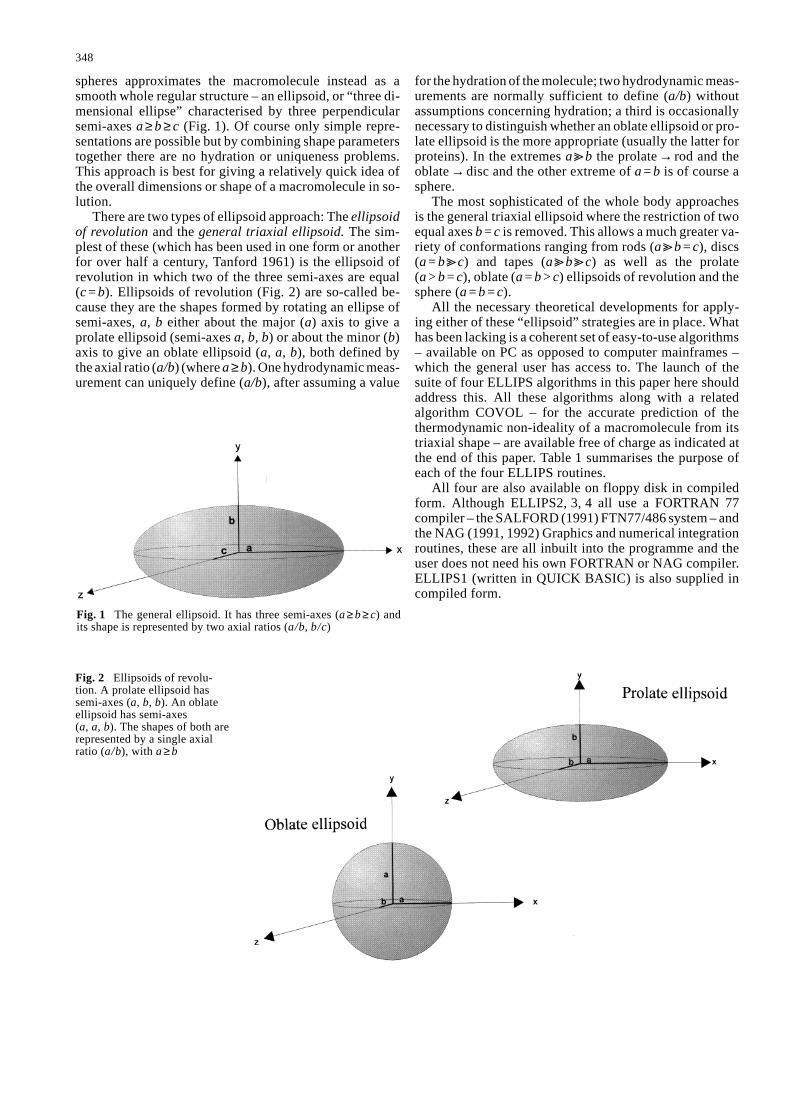
spheres approximates the macromolecule instead as asmooth whole regular structure – an ellipsoid, or “three di-mensional ellipse” characterised by three perpendicularsemi-axes a ≥ b ≥ c (Fig. 1). Of course only simple repre-sentations are possible but by combining shape parameterstogether there are no hydration or uniqueness problems.This approach is best for giving a relatively quick idea ofthe overall dimensions or shape of a macromolecule in so-lution.

There are two types of ellipsoid approach: The ellipsoidof revolution and the general triaxial ellipsoid. The sim-plest of these (which has been used in one form or anotherfor over half a century, Tanford 1961) is the ellipsoid ofrevolution in which two of the three semi-axes are equal(c = b). Ellipsoids of revolution (Fig. 2) are so-called be-cause they are the shapes formed by rotating an ellipse ofsemi-axes, a, b either about the major (a) axis to give aprolate ellipsoid (semi-axes a, b, b) or about the minor (b)axis to give an oblate ellipsoid (a, a, b), both defined bythe axial ratio (a/b) (where a ≥ b). One hydrodynamic meas-urement can uniquely define (a/b), after assuming a value

for the hydration of the molecule; two hydrodynamic meas-urements are normally sufficient to define (a/b) withoutassumptions concerning hydration; a third is occasionallynecessary to distinguish whether an oblate ellipsoid or pro-late ellipsoid is the more appropriate (usually the latter forproteins). In the extremes a ob the prolate → rod and theoblate → disc and the other extreme of a = b is of course asphere.

The most sophisticated of the whole body approachesis the general triaxial ellipsoid where the restriction of twoequal axes b = c is removed. This allows a much greater va-riety of conformations ranging from rods (a ob = c), discs(a = b oc) and tapes (a ob oc) as well as the prolate(a > b = c), oblate (a = b > c) ellipsoids of revolution and thesphere (a = b = c).

All the necessary theoretical developments for apply-ing either of these “ellipsoid” strategies are in place. Whathas been lacking is a coherent set of easy-to-use algorithms– available on PC as opposed to computer mainframes –which the general user has access to. The launch of thesuite of four ELLIPS algorithms in this paper here shouldaddress this. All these algorithms along with a related algorithm COVOL – for the accurate prediction of the thermodynamic non-ideality of a macromolecule from itstriaxial shape – are available free of charge as indicated atthe end of this paper. Table 1 summarises the purpose ofeach of the four ELLIPS routines.

All four are also available on floppy disk in compiledform. Although ELLIPS2, 3, 4 all use a FORTRAN 77compiler – the SALFORD (1991) FTN77/486 system – andthe NAG (1991, 1992) Graphics and numerical integrationroutines, these are all inbuilt into the programme and theuser does not need his own FORTRAN or NAG compiler.ELLIPS1 (written in QUICK BASIC) is also supplied incompiled form.

348

Fig. 1 The general ellipsoid. It has three semi-axes (a ≥ b ≥ c) andits shape is represented by two axial ratios (a/b, b/c)

Fig. 2 Ellipsoids of revolu-tion. A prolate ellipsoid hassemi-axes (a, b, b). An oblateellipsoid has semi-axes(a, a, b). The shapes of both arerepresented by a single axial ratio (a/b), with a ≥ b

Universal shape functions: hydration dependent and hydration independent

Before we consider each routine in detail we will summar-ise the hydrodynamic shape functions involved. To be con-sistent with the bead modelling programme SOLPRO wecall these Universal Shape Functions. By this we meaneach is specifically a function of shape alone (and not vol-ume): it makes no odds what the size is: a Universal shapefunction will have the same value, it will only depend onthe shape. All these universal shape functions have beenworked out in terms of the axial ratio (a/b) for ellipsoidsof revolution and now the two axial ratios (a/b, b/c) forgeneral ellipsoids. All of these (with the exception of theexclusion volume based shape functions ured and Π ) arealso available for bead models from SOLPRO (Garcia dela Torre et al. 1997). For all the ellipsoid formulae the useris referred to Harding (1995) and references therein andfor all the bead formulae the user is referred to Garcia dela Torre et al. (1997) and references therein. However, theinvestigator need not concern himself with these: all ofthese formulae are inbuilt into the ELLIPS routines in thecase of ellipsoid modelling and SOLPRO in terms of beadmodelling. In terms of the experimental measurement ofthese Universal shape functions, some require knowledgeof the hydration δ (mass in g of H2O bound per g of drymacromolecule) or hydrated volume V (ml) of the particle,the others do not. The particle volume V is often presentedin two equivalent forms:

V = vs · M/NA (1)

where M is the molecular weight or molar mass (g/mol)and NA is Avogadro’s number (6.02205 × 1023 mol–1), andvs is the specific volume (ml/g) of the hydrated macromole-cule (volume occupied by the hydrated macromolecule perunit mass of dry macromolecule) or

V = (v– +δ /ρ0) · M/NA (2)

where v– is the partial specific volume (ml/g).

Hydration dependent universal shape functions

Those Universal shape functions requiring knowledge ofδ or V for their experimental measurement are:

– Viscosity increment, ν (Simha 1940; Saito 1951)

ν = [η] M/ (NAV ) (3)

ν = 2.5 for a sphere (Einstein 1906, 1911)

– Perrin function, P (Perrin 1936)

P = ( f /f0) /{1 + δ /(v–ρ0)}–1/3 (4)

where ( f /f0), the frictional ratio (Tanford 1961) is relatedto the sedimentation coefficient s 0

20,w by

( f /f0) = M (1 – v–ρ0)/(NA · 6 π η0 s020,w) (4 π NA /3 v–M)1/3 (5)

or the translational diffusion coefficient D 020,w by

(6)

where T = 293.15 K, η0 is the viscosity of water at 293.15 K (0.010 Poise), ρ0 is the density of water at 293.15 K (0.99823 g/ml) and kB is Boltzmann’s constant(1.3807 × 10–16 erg. K–1). P = 1 for a sphere (Perrin 1936)

– Reduced excluded volume, ured

ured = u /V = {2 B M 2 – Z2/2 I}/ (NAV ) (7)

u is the excluded volume (ml), B is the second thermo-dynamic (or “osmotic pressure”) virial coefficient, fromosmotic pressure, light scattering or sedimentation equi-librium measurements, Z is the valency of the macro-molecule, measurable by titration (Jeffrey et al. 1977) andI is the ionic strength of electrolyte in the solvent (mol/ml).At sufficient ionic strengths, the Z2/2 I term becomes neg-ligible compared with 2B M 2. Of course for unchargedmacromolecules and proteins at the isoelectric point Z = 0.ured = 8 for a sphere (Tanford 1961)

– Harmonic mean rotation relaxation time ratio:

τh /τ0 = {kB T /η0V} · τh (8)

where τh (sec) is the harmonic mean rotational relaxationtime, traditionally measured using steady state fluores-

( / )/

,f f

k T NM D

B A0

0

1 3

2006

43

1=

⋅π η

πv w

349

Table 1 The ELLIPS routines

Routine Language Model Purpose

ELLIPS1 QUICKBASIC Ellipsoid of Revolution Prediction of axial ratio (a/b) (equivalent prolate or oblate ellipsoid of revolution) from user specified shape function

ELLIPS2 FORTRAN 77 General Triaxial Ellipsoid Evaluates the values of all the hydrodynamic shape functions from user specified (a, b, c) or (a/b, b/c)a

ELLIPS3 FORTRAN 77 General Triaxial Ellipsoid Evaluates (a/b, b/c) from combinations of hydration independent shape functions

ELLIPS4 FORTRAN 77 General Triaxial Ellipsoid Evaluates (a/b, b/c) from electro-optic decay combined with other hydrodynamic data

a Equivalent to SOLPRO (Garcia de la Torre et al. 1997) for bead models

cence depolarisation methods (Van Holde 1971, 1985), andτ0 the corresponding value for a spherical particle of thesame volume:

τ0 = η0V/kB T (9)

In earlier representations a factor of 3 was introduced be-cause the rotational relaxation time was referred to on adielectric dispersion basis (compensated for in the equa-tions for steady state anisotropy depolarisation) althoughthis is no longer necessary – compare van Holde (1971)with van Holde (1985). This is further discussed in Garciade la Torre et al. (1997). τh /τ0 = 1 for a sphere (Perrin 1934).

– Time-resolved rotational (fluorescence depolarisationanisotropy) relaxation time ratios

τk /τ0 = {kB T /η0V ) · τk (10)

For ellipsoids of revolution k = 1–3; for general ellipsoidsand general particles, k = 1–5. τk /τ0 = 1 for a sphere (Smalland Isenberg 1977).

– Reduced electro-optic decay constants

θ ired = (η0V /kB T ) · θi (11)

where θi are the electric birefringence or electric dichro-ism decay constants. For ellipsoids of revolution that arehomogeneous i.e. where the geometric axis of symmetrycoincides with the electrical axis, i = 1. For general ellip-soids that are homogeneous i.e. where the geometric axescoincide with the electrical axes, i = 2, termed “+” and “–”(Ridgeway 1966, 1968); for general particles i = 1–5 (Wegener et al. 1979). For a sphere, θ i

red = 0.66667.

Hydration independent universal shape functions

Those Universal shape functions NOT requiring knowl-edge of δ or V for their experimental measurement are:

– Scheraga-Mandelkern (1953) parameter

(12)

The β parameter is unfortunately very insensitive to shape,and Eq. (12) is used more as an equation of consistency,or for measuring M from sedimentation velocity and vis-cosity measurements. β = 2.1115 × 106 for a sphere

– Pi function (Harding 1981a)

Π = {2B M /[η]} – {Z2/2 I M [η]} = ured/ν (13)

with the 2nd term (a good approximation of the charge contribution for polyelectrolytes) → 0 at sufficient valuesof I, and of course = 0 for uncharged macromolecules or proteins at the isoelectric point (Z = 0). Π = 3.2 for asphere

– Wales-van Holde (1954; Rowe 1977) parameter

R = ks /[η] = 2 (1+ P3) /ν (14)

β η ηρ π

ν≡−

=[ ]( ) ( )

./

/ /

/

/

/1 30

2 30

1 3

1 3

2 1 3

1 3

1 100 16200M

NP

A

v

where ks (ml/g) is the concentration dependence parame-ter of the sedimentation coefficient in the limiting relations20,w = s 0

20,w (1 – ks c) or 1/s20,w = {1/s 020,w} (1 + ks c). Al-

though the theory behind Eq. (14) is less rigorous than thatfor Π (because of the greater complexity of “hydrody-namic” as opposed to “thermodynamic equilibrium” basednon-ideality), it does have a strong experimental basis (Creeth and Knight 1965; Rowe 1977, 1992). To apply ksin this way it is important that charge contributions to ksare absent or if the macromolecule is a polyelectrolyte,charge contributions are suppressed by working in a sol-vent of sufficient ionic strength. R = 1.6 for a sphere.

– Reduced radius of gyration function G (Harding 1987)

G = Rg2 · {4π NA / (3v M )}2/3 (15)

where Rg is the radius of gyration (cm), from light scatter-ing, x-ray scattering or neutron scattering measurements.Provided that there is no difference in scattering density ofthe surface bound solvent compared with free solvent, andthere is no significant internal swelling of the macromol-ecule, we can take, to a good approximation, v ~ v–. Other-wise G must also be treated as another hydration depen-dent parameter. G = 0.6 for a sphere.

– Psi-function (Squire 1970)

(16)

For spheres, Ψ = 1. It should be stressed that Ψ, like β isvery insensitive to shape and is more use as an equation ofconsistency. Ψ = 1 for a sphere.

– Lambda function (Harding 1980a)

Λ = (η0 · [η] · M ) / (NA · kB T τh) = ν /(τh /τ0) (17)

For spheres, Λ = 2.5.

– Lambda and psi functions for each relaxation time (Garcia de la Torre et al. 1997)

Λk = (η0 · [η] · M ) / (NA · kB T τk) = ν /(τk /τ0) (18)

(19)

(k = 1–3 for ellipsoids of revolution; 1–5 for general tri-axial ellipsoids). For spheres, Ψk = 1 and Λk = 2.5.

– Electro-optic delta and gamma (Harding and Rowe1983) functions

δi = (6η0/NA kB T ) [η] M · θi = 6 θ ired ν (20)

γ i = (M 3(1 – v–ρ0)3/ (27N 3A kB T π2η0

2 s020,w

3 ))· θi = 6 θ i

red P3 (21)

(for homogeneous ellipsoids of revolution i = 1 and for homogeneous triaxial ellipsoids, i = “+” and “–”). Forspheres, γ i = 1.0 and (the more sensitive) δi = 2.5.

ΨkA k

kkTM

N sP=

−

=43

1

610

1 30

0 200

1 3

01 3π η ρ

π η ττ τ

/

,

//( )

/( / )v

w

Ψ =

−

=43

16

101 3

0

0 200

1 3

01 3π η ρ

π η ττ τ

kTM

N sP

A hh

/

,

//( )

/( / )v

w

350

ELLIPS1

Aim. Prediction of axial ratio (a/b) (equivalent prolate oroblate ellipsoid of revolution) from a user specified valuefor a shape function.

Description. ELLIPS1 is based on simple ellipsoid of rev-olution models (where two of the three axes of the ellip-soid are fixed equal to each other); if the user types in avalue for a shape function from sedimentation or othertypes of hydrodynamic measurement, it will return a valuefor the axial ratio of the ellipsoid. The question an exper-imenter wishes to address usually is not “what is the shapefunction for a specified value of the axial ratio a/b?” butrather “what is the axial ratio a/b for my macromoleculespecified by my (Universal) shape function which I haveexperimentally measured?”. Unfortunately, although thereare exact analytical formulae linking each shape functionwith a/b (Harding and Cölfen 1995), the reverse is not true:inversion is analytically impossible. In the past, the inves-tigator has had to interpolate from tables of data (Hardingand Cölfen 1995) or from graphs to obtain his a/b from P(obtained from the sedimentation or diffusion coefficient),ν (from the intrinsic viscosity), R, Π, Λ etc. Harding andCölfen (1995) have provided a simple polynomial basedinversion procedure giving a/b versus the various Univer-sal shape functions to an acceptable degree of accuracy(i.e. to better than the precision of the measurement, whichis normally no better than a few percent) and within thelimits of the assumption that an ellipsoid of revolutionshape is a reasonable approximation of a macromolecule.The polynomial formulae used is simply

(a/b) = a0 + Σi

ai xi (22)

with x = P, ν, β, R, Π or Λ and for both prolate and oblateellipsoids in each case.

The fits are split into 3 ranges: Range 1 (1.1 < a/b < 2.0);Range 2 (2 < a/b < 10) and Range 3 (10 < a/b < 100) and apolynomial of degree 7 or less is necessary to give a goodto excellent fit (by this we mean the fit is at least as goodas the precision to which the function can be measured –usually to no better than a few percent). The only excep-tions are the relatively uninteresting cases of prolate βrange 1, oblate β range 2, oblate β range 3 and oblate Πrange 1: in these cases the ELLIPS routine returns the warn-ing “POOR FIT: USE GRAPHICAL INTERPOLATION”.Some functions do not distinguish between prolate andoblate ellipsoids: in this case the a/b values for both casesare returned and the user has to choose between the two.For proteins the prolate usually gives the closest represen-tation. All the coefficients in Eq. (22) for each function foreach range and for both prolate and oblate ellipsoids aregiven in Harding and Cölfen (1995), although again, theuser need not concern himself with these since they are in-built into the compiled program.

Output. Figure 3 gives the user screens for an example runon the protein egg albumin using two of the hydration in-

dependent universal shape functions (a) the Pi function and(b) the R-function. In the case of (a), Π = 3.18 {fromBM = 5.55 ml/g and [η] = 3.49 ml/g (Z2/2 I ~ 0)}: this givesan a/b ~ 1.5 but after experimental error it could be any-thing between 1 and 3. However, use of the R function (b),which is very sensitive for particles of low asymmetry confirms this value for the axial ratio for ovalbumin (eggalbumin). Interestingly this finding of 1981 (Harding1981b) was confirmed from the crystal structure (Fig. 3c)published 10 years later (Stein et al. 1991). More interest-ingly the axial ratio of a size 3 U.K. standard egg (Fig. 3d)is also ~1.5.

Although the MSDOS (Microsoft, Redmond, Washing-ton, USA) routine can only draw a crude 2D representa-tion of the structure, CORELDRAW (Corel Co., Ontario)will give a 3D presentation (Fig. 3c).

ELLIPS2

Aim. Evaluates the values of all the Universal hydrody-namic shape functions from user specified axial dimen-sions (a, b, c) or axial ratios (a/b, b/c) for the macromole-cule as modelled by a general triaxial ellipsoid.

Description. ELLIPS2 is essentially analagous to SOL-PRO (Garcia de la Torre et al. 1997) in that from a givenstructure (as represented by an array of beads in SOLPROor as a general triaxial ellipsoid in ELLIPS2) the completeset of Universal shape functions is returned. ELLIPS2 also evaluates the excluded volume shape functions uredand Π, unavailable on SOLPRO. It is based on an earlierversion of the program written in FORTRAN for main-frame computer (Harding 1982). The earlier version alsolacked ured and Π for the simple reason these hadn’t beenworked out for triaxial allipsoids until 1985 (Rallison andHarding 1985).

Most of the universal shape functions involve one ormore of 10 different elliptic integrals (called alpha 1 …alpha 10 – see Harding 1995) of the form

∫∞

0f (x) dx (23)

There is still no packaged or published numerical routineavailable for integrals of this type; only routines of the form

∫B

Af (x) dx (24)

where A can be zero but B must have a finite value, spec-ifiable by the user. ELLIPS2, like its mainframe fore-runner uses a NAG (1991) quadrature routine, in this caseD01AJF. B can be set as high as the programmer wishes:higher values take more computer time though, and in prac-tice, satisfactory convergence of the integral is obtained ifB is set to 106 for 9 of the intergrals (alpha1– alpha9) and108 for the remaining alpha10. It is also found that eachintegration is best split into 2 parts: part 1 (between A = 0and B = 100) and part 2 (A = 100, B = 106 or 108). D01AJF

351

also requires the following settings: epsabs = 0.0; epsrel= 0.5 × 10–4. ured and Π also require numerical integra-tions, this time for two double integrals of the form

∫0

π /2

∫0

π /2

f (x1, x2) dx2 dx1 (25)

where f (x1, x2) is a complicated transcandental function inboth cases. Analytical solutions are not possible, so theNAG routine D01DAF is employed. This quadrature rou-

tine performs a two-dimensional integral and has the set-ting absacc = 1.0 × 10–5.

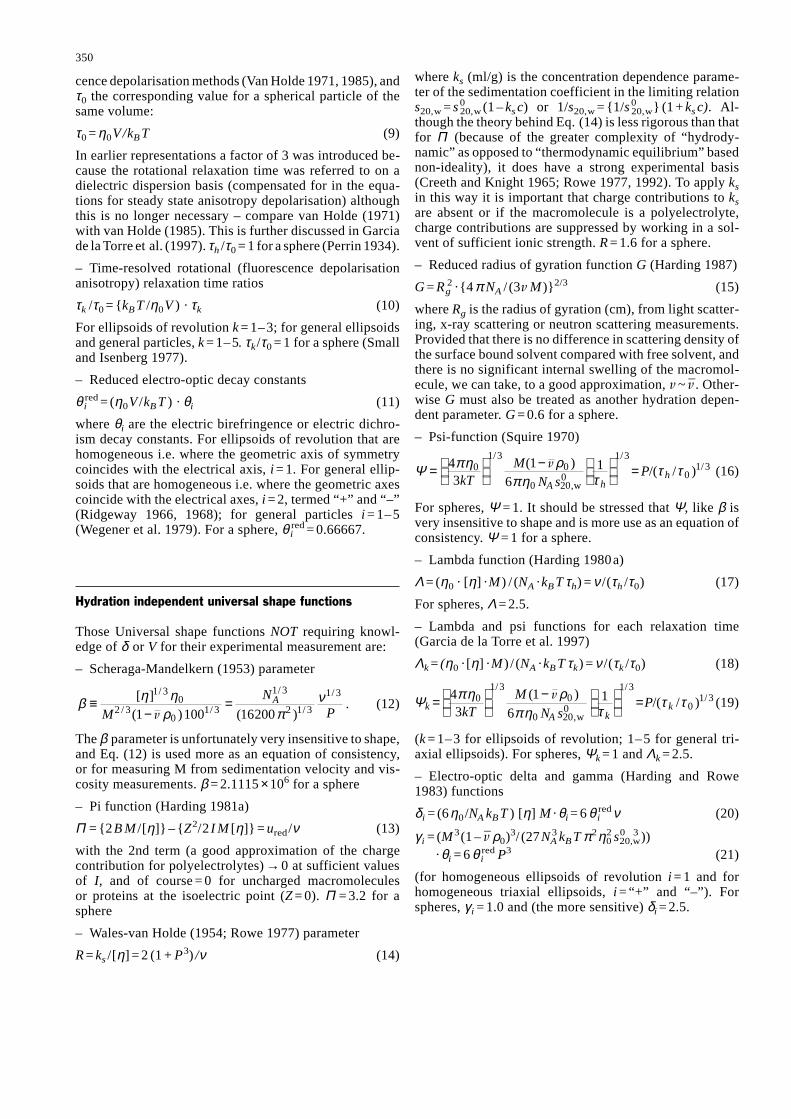
Output. Fig. 4 (a) gives the output data for an (a/b,b/c) = (1.23, 1.52), based on the crystallographic axial di-mensions of 43 × 35 × 23 Å for myoglobin (Kendrew et al.1958) (Fig. 4b). Besides giving the excluded volume basedured and Π, the Λk and Ψk (k = 1 → 5) shape parameters aregiven, instead of the less useful “rotational frictional ra-tios”.

A spin-off of this routine is another called COVOL (which will be described elsewhere): this uses the predictedvalue of ured to evaluate the second theromodynamic vir-ial coefficient B, as an aid to the prediction of the non-ideality terms which appears in analyses of molecular inter-action phenomena using light scattering or sedimentationequilibrium.

352

a b

c d

Fig. 3 ELLIPS1 output screens for the determination of the axialratio (a/b) for ovalbumin (egg albumin) using the Universal shapefunctions (a) Π or (b) R. (c) Prolate ellipsoid of a/b = 1.5 drawn bythe WINDOWS based CORELDRAW enclosing the crystal struc-ture line-drawing of Stein et al. (1991). (d) A standard egg ofa/b ~ 1.5

ELLIPS3

Aim. Evaluates the tri-axial shape of a macromolecule (a/b,b/c) using two possible combinations of Universal hydra-tion independent shape functions:

(a) Π (from the second virial coefficient and intrinsic vis-cosity measurements) with G (from radius of gyrationmeasurements), or(b) Λ (from the harmonic mean rotation relaxation time τhand intrinsic viscosity [η] measurements) with R (from theconcentration dependence sedimentation term ks and in-trinsic viscosity measurements).

Description. Whereas an (a/b, b/c) specifies uniquely val-ues for all the hydrodynamic shape functions, the reverseis unfortunately not true: measurement of P, R, Λ etc. doesnot uniquely fix (a/b, b/c) but rather gives a line solution

353

a

b

Fig. 4 a ELLIPS2 output for a macromolecule of axial ratios(a/b, b/c) = (1.23, 1.52) (myo-globin). b Ellipsoidal represen-tation of the crystal structure ofmyoglobin (a/b, b/c) = (1.23,1.52) {based on axial dimen-sions of 45 × 35 × 23 Å (Ken-drew et al. 1958) and line draw-ing of Dickerson and Geis(1969)}

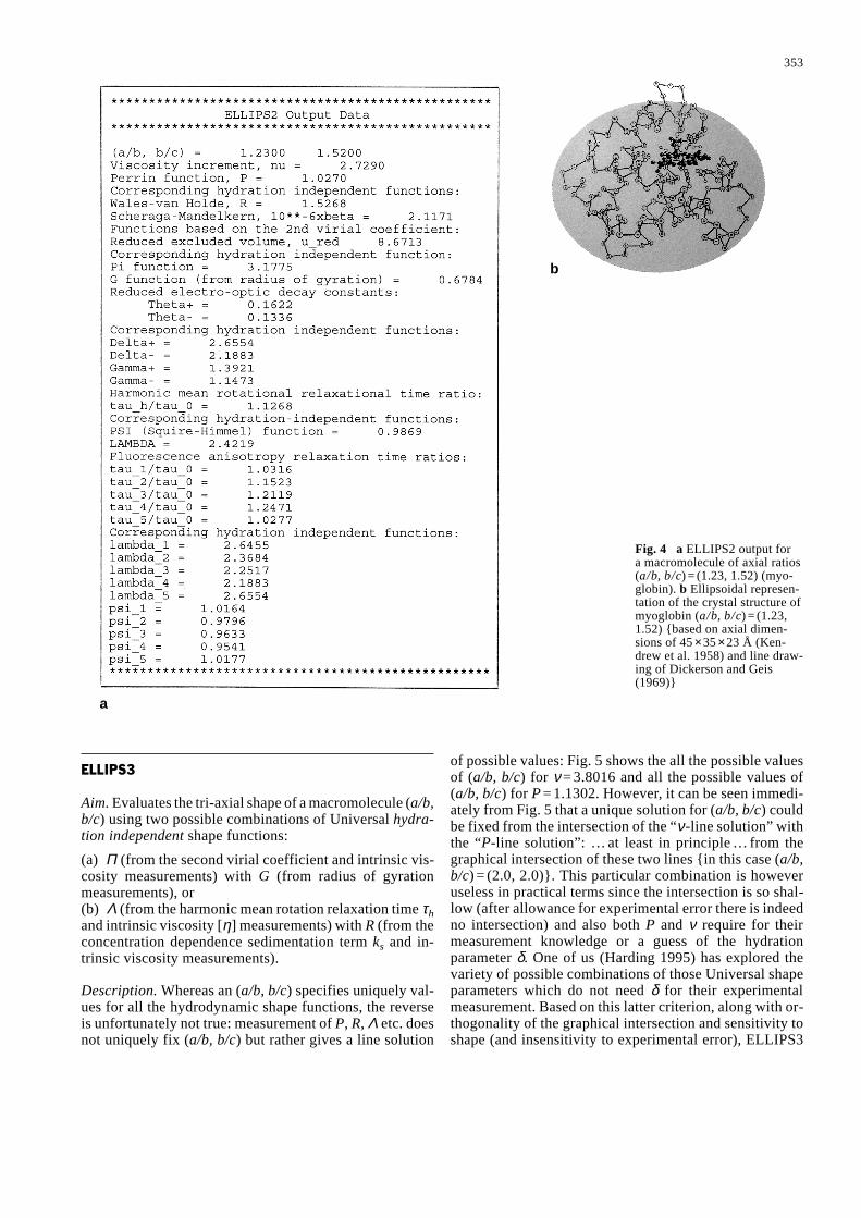
of possible values: Fig. 5 shows the all the possible valuesof (a/b, b/c) for ν = 3.8016 and all the possible values of(a/b, b/c) for P = 1.1302. However, it can be seen immedi-ately from Fig. 5 that a unique solution for (a/b, b/c) couldbe fixed from the intersection of the “ν-line solution” withthe “P-line solution”: … at least in principle … from thegraphical intersection of these two lines {in this case (a/b,b/c) = (2.0, 2.0)}. This particular combination is howeveruseless in practical terms since the intersection is so shal-low (after allowance for experimental error there is indeedno intersection) and also both P and ν require for theirmeasurement knowledge or a guess of the hydration parameter δ. One of us (Harding 1995) has explored thevariety of possible combinations of those Universal shapeparameters which do not need δ for their experimentalmeasurement. Based on this latter criterion, along with or-thogonality of the graphical intersection and sensitivity toshape (and insensitivity to experimental error), ELLIPS3

provides for 2 of the most promising combinations. Thefirst is a combination of Π (from the second thermody-namic virial coefficient and intrinsic viscosity) with G(from x-ray, neutron or light scattering), the second is acombination of Λ (from steady state fluorescence depola-rization measurements and the intrinsic viscosity) with R(from the concentration dependence sedimentation term ksand intrinsic viscosity measurements).

ELLIPS3 uses as its basis the function calculation rou-tine of ELLIPS2 except that a whole array of such valuesare evaluated in the (a/b, b/c) plane (a matrix of 40 × 40values). A Contour plotting routine (J06GAF in the NAGFORTRAN Library) interpolates between these matrixpoints and can plot the Π, G, Λ and R functions (or anyother of the universal shape functions if the programmerso decides) in the (a/b, b/c) plane. In the pre-compiled ver-sion available for ELLIPS3, the user does not have to con-cern himself with the details behind the program if he ishappy with either the Π –G or Λ –R combinations.

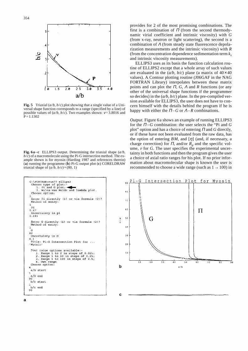
Output. Figure 6a shows an example of running ELLIPS3for the Π –G combination: the user selects the “Pi and Gplot” option and has a choice of entering Π and G directly,or if these have not been evaluated from the raw data, hasthe option of entering BM, and [η] (and, if necessary, acharge correction) for Π, and/or Rg and the specific vol-ume, v for G. The user specifies the experimental uncer-tainty in both functions and then the program gives the usera choice of axial ratio ranges for his plot. If no prior infor-mation about macromolecular shape is known the user isrecommended to choose a wide range (such as 1 → 100) in

354

Fig. 5 Triaxial (a/b, b/c) plot showing that a single value of a Uni-versal shape function corresponds to a range (specified by a line) ofpossible values of (a/b, b/c). Two examples shown: ν = 3.8016 andP = 1.1302

a

b

c

Fig. 6a–c ELLIPS3 output. Determining the triaxial shape (a/b,b/c) of a macromolecule using the Pi-G intersection method. The ex-ample shown is for myosin (Harding 1987 and references therein)(a) running the programme (b) Pi-G output plot (c) CORELDRAWtriaxial shape of (a/b, b/c) = (80, 1)

the first instance, and then replot at higher resolution in therange of interest. The myosin example is given to showthat, without any prior assumptions about the conforma-tion (rod, sphere disc, etc.) and despite hinge regions oflimited flexibility in the molecule and the presence of theS1 protrusions at one end, the overall gross conformationof a rod shape of axial ratio ~80 :1 is returned.

The second example of ELLIPS3 (Fig. 7) is for the Λ –R plot applied to the neural protein neurophysin: de-

tails of how [η], τh and ks was extracted for both monomersand dimers is described in Nicolas et al. (1981) and alsoHarding and Rowe (1982). Figure 7a shows the running ofELLIPS3 for Λ –R and Fig. 7b and c the output for themonomers and dimerised form of the protein, with the lat-ter clearly indicating that when the 4 :1 prolate ellipsoidalmonomers dimerise they must do so in a side-by-side asopposed to end-on process.

355

b

c

a

Fig. 7a–c ELLIPS3 output.Determining the triaxial shape(a/b, b/c) of a macromoleculeusing the Λ-R intersectionmethod. The example shown isfor neurophysin (Harding andRowe 1982 and referencestherein) (a) running the pro-gramme (b) Λ-R plot for neuro-physin monomers (inset – CORELDRAW ellipsoid of(a/b, b/c) = (4,1)) (c) Λ-R plotfor neurophysin dimers yield-ing (a/b, b/c) = (2.5, 2.85) {in-set shows likely mode of as-sembly of the monomers}

ELLIPS4

Aim. Evaluates the tri-axial shape of a macromolecule (a/b,b/c) from electro-optic decay based Universal shape func-tions combined with other hydrodynamic data.

Description. Rotational hydrodynamic shape functions,based around rotational diffusion measurements are attrac-tive for determining the shapes of macromolecules in so-lution since they are generally more sensitive functions ofshape compared to other shape functions. This sensitivitycomes however at a price because they are generally mo-re difficult to measure. A lot of the difficulty centres aroundresolution of multi-exponential decay functions. Electro-optic measurements are more attractive than time-resolvedfluorescence depolarization anisotropy measurements inthe sense that for homogeneous triaxial ellipsoids at least,there are only two exponential terms to resolve (the decayconstants or reciprocal relaxation times θ+ and θ–) as op-posed to five (τ1 – τ5):

∆n = A′+ exp (–6θ+ t) + A′– exp (–6θ– t)

(Ridgeway 1968, Harding and Rowe 1983) where ∆n isthe birefringence or dichroism (often expressed as “opti-cal retardation” in degrees) at time t after the aligningelectric field has been switched off. A practical problemwith electro-optic decay methods is the potential local heat-ing effects from the high electric fields used, especially ifthe experiments are conducted in solutions of high ionicstrength: the investigator is advised to consult an article byPorschke and Obst (1991) describing how these effects canbe minimised.

After eliminating hydration (via e.g. combination with[η]) to give the Universal hydration independent shapefunctions δ+ and δ– and graphical combination with an-other Universal hydration independent shape function suchas R (Harding and Rowe 1983) or Π (Harding 1986) thetriaxial shape as represented by the two axial ratios (a/b,b/c) can be evaluated. Resolution however of even two ex-ponential terms is not easy, particular for globular macro-molecules where θ+ and θ– are similar (Small and Isenberg1977), and no-matter what form of mathematical decon-volution is applied, whether it be non-linear least squaresor more refined types of analysis (Harding 1980b; Jost andO’Konski 1978; O’Connor et al. 1979; see Johnsen andBrown (1992) for the analagous problem in dynamic lightscattering analysis of polydisperse systems). In our hands(Harding 1980b; Harding and Rowe 1983) we have founda more reliable method of extraction is to use another hy-drodynamic function as a constraining parameter in theanalysis of the electro-optic decay data: in this way theproblem is reduced to one of four variables (A′+, θ+, A′–, θ–)to one of three (A′+, A′–, a/b) since a/b will specify, by theconstraining function a unique value for b/c (and henceθ+,θ–). ELLIPS4 has been written to facilitate this proce-dure for PC based on an earlier non-interactive version ofthe programme written for mainframe computer (Harding1980b, 1983). Its use is best illustrated by application to

synthetic data (with error) generated for a macromolecule“Protein 1” (Harding and Rowe 1983) which includes the following characteristics: (a/b, b/c) = (1.5, 1.5);M = 71744 Da; [η] = 2.74 ml/g, and the following electro-optic decay parameters: = A′+ = 0.07, A′ = 0.05, θ+ =5.81538× 106 s–1, θ– = 4.15646 × 106 s–1, T = 293.15 K, η0 = 0.01Poise. Figure 8 shows the electro-optic decay for this basedon expected error (standard deviation) of ±0.1 degrees (optical retardation) or ±0.0017 rads random normal erroron the decay data.

With ELLIPS4 the user puts his electro-optic decay data(∆n versus t) into a data file which is read in. The user alsohas to specify values for [η] (ml/g), the molecular weightM (Da), the solvent viscosity (Poise) and temperature (K)at which the electro-optic measurements were made. Theuser also needs to specify the coordinates of a line of (a/b,b/c) values (based on measurement of R, Π or some otherhydration independent Universal shape function) in a sec-ond data file: Fig. 9 shows such a constraining line of al-lowed (a/b, b/c) values for “Protein 1” which has an R-function value of 1.479. This constrains each iteration of(a/b, b/c) and hence θ+, θ–, to work along the line speci-fied by the constraining function, since each value of (a/b,b/c) specifies a value for δ+ and δ– – (worked out using thesame procedure involving the NAG routine D01AJF usedin ELLIPS2 and 3) which, combined with the user enteredvalues for T, η0, [η] and M gives the θ+, θ– for each itera-tion. This reduces the risk of the fitting routine falling intosubsidiary minima. When the minimum of the least squaresprocedure has been formed ELLIPS4 successfully returnsa/b, its corresponding value of b/c and the pre-exponentialfactors A′+ and A′–. The programme runs automatically 4times using successively the 4 different values of a/b en-tered from the constraining function (excluding the firstand last data points) as starting estimates for a/b: this pro-vides a further check against the dangers of subsidiary min-ima. For the starting estimates for A′+ and A′– the routineautomatically takes these as ∆nmax/2. The routine has in-built various error warnings concerning the reliability ofeach estimation. If no error warning is returned the result

356

Fig. 8 Electro-optic decay (expressed as the decay of optical retar-dation with time, t [s]). Synthetic data shown corresponding to a pro-tein of true (a/b, b/c) = (1.5, 1.5) {“Protein 1” of Harding and Rowe1983}. The electro-optic data is fed in as a date-file into ELLIPS4

for the evaluation from a particular starting point shouldbe reliable.

Output. Figure 10 shows (a) the running of the programmeand (b) the output for a run on the data of Fig. 8 for Pro-tein 1, which returns a value for (a/b, b/c) ~ (1.62, 1.34) –

i.e. to within two tenths of an axial ratio unit of the trueaxial ratios. In practical terms however, the user is advisedto (i) repeat the whole operation several times with vari-ous cut-off times for the decay data (at longer times thesignal/noise data gets progressively worse, on the otherhand more information concerning the slower relaxationtime, or larger decay constant, θ+ is contained in this re-gion) to be certain of no subsidiary-minima problems (ii)repeat the operation allowing for experimental error in theconstraining function (iii) check for any concentration de-pendence of the returned parameters: and extrapolate ifnecessary to zero concentration (Riddiford and Jennings1967). These and other features have been extensively ex-plored with the earlier mainframe version of the pro-gramme (Harding 1980b; Harding 1983; Harding and Rowe 1983). A possible area of further improvement includes the additional constraint that A′+ + A′– = ∆nmaxalthough this may cause problems if the data is noisy andthe t = 0 position is not precisely defined.

Concluding comment

All the routines ELLIPS1, 2, 3 and 4 are available on diskor via email/ftp as explained below and all should be sim-ple to use. The user ultimately however has to decide justhow far he wants to take his hydrodynamic conformationdeterminations on a macromolecule, assuming it is fairlyrigid (if the molecule fails this criterion then there are other

357

Fig. 9 ELLIPS4 constraining data extraction. The user takes his de-termined value of R or other suitable constraining function (Π, G, Λetc.) and plots the line of corresponding values of (a/b, b/c) usingELLIPS3 (ELLIPS3 gives 2 lines which allow for experimental er-ror, both of which can be used in successive runs using ELLIPS4. Italso plots 2 lines for a 2nd function which should be entered = 0).The user then reads off 6 (a/b, b/c) coordinates from this line whichcan be either entered as a 2nd data file into ELLIPS4, or instead en-tered at run-time

Fig. 10a, b ELLIPS4: Determining the triaxial shape (a/b, b/c) ofa macromolecule using electro-optic decay data. Illustrated by ap-plication to “Protein 1” of true (a/b, b/c) = (1.5, 1.5) and based onthe electro-optic decay data of Fig. 8 and constraining line solutionof Fig. 9. a Running the programe. The user needs to enter valuesfor the temperature, solvent viscosity, intrinsic viscosity [η] of themacromolecule and the molecular weight M. The programme runs 4 times with the constraining values (a/b, b/c) {excluding the firstand last point) as the initial estimates. b Output giving the returnedvalues for (a/b, b/c) and the pre-exponential factors for each of thefour starting estimates for (a/b, b/c) and the final “best” result. Alist of potential error warning estimates is also given

procedures available, as reviewed by Harding 1995). Ellipsoids of revolution – via the routine ELLIPS1 give arelatively quick impression of the overall form of the mole-cule (providing a distinction as to whether its best mod-elled by a prolate or oblate can be made). Although gen-eral ellipsoid modelling, using ELLIPS2, like bead mod-elling using SOLPRO (Garcia de la Torre et al. 1997) cannow easily predict the hydrodynamic properties of a mac-romolecule of given shape: the reverse is more difficult.With SOLPRO the problems are one of uniqueness (i.e. themultiplicity of models which yield the same set of hydro-dynamic parameters); ELLIPS3 and 4 circumvent theseuniqueness problems but only by forgoing molecular de-tail and using a graphical extraction strategy, with undoubt-edly ELLIPS3 the easiest to perform.

Whatever he does the investigator needs to moderatehis desire for high precision with a sense of realism:whether it be ellipsoids or beads, these are only approxi-mations to the true conformation of a macromolecule (thehydrodynamic theory behind the latter is also only an ap-proximation); even though the so-called hydration prob-lem can be countered with the use of those Universal shapefunctions which are hydration-independent, there is still afurther assumption (usually reasonable) that the hydrationof a macromolecule is ~ the same for different measure-ments. Because of these reasons, hydrodynamics will always be a so called “low” or “fairly-low” resolution ap-proach to conformation analysis.

Nonetheless, the relative speed with which the meas-urements can be performed, coupled with the limitationsof the so-called “high-resolution” techniques (which inmany instances cannot be applied and can never be appliedanyway to a molecule in dilute solution) make modern hy-drodynamic conformation algorithms highly attractive as“overall solution structure” (ellipsoids) or “solution mo-lecular refinement” (beads) algorithms.

Program availability The ELLIPS programs are available. Free atcharge either directly from the authors (email: steve.harding@not-tingham.ac.uk or coelfen@mpikg-teltow.mpg.de) or from the Inter-net. Log in as anonymous ftp on BBRI.HARVARD.EDU and thenchange to /RASMB/SPIN/MS_DOS/ELLIPS-HARDING.

References

Creeth JM, Knight CG (1965) Biochim Biophys Acta 102:549–558Dickerson RE, Geiss I (1969) The structure and action of proteins.

Harper and Row, New York, p 47Einstein A (1906) Eine neue Bestimmung der Molekuldimensionen.

Ann Physik 19:289–305Einstein A (1911) Berichtigung zu meiner Arbeit: „Eine neue Be-

stimmung der Molekulardimensionen“. Ann Physik 34:591–593Eisenberg H (1976) Biological Macromolecules and Polyelectroly-

tes in Solution. P25. Clarendon Press, OxforGarcia de la Torre J, Bloomfield VA (1977) Hydrodynamic properties

of macromolecular complexes I. Translation. Biopolymers 16:1747–1763

Garcia de la Torre J, Navarro S, Lopez Martinez MC, Diaz FG, Lopez Cascales JJ (1994) HYDRO: A computer software for the prediction of hydrodynamic properties of macromolecules.Biophysical J 67:530–531

Garcia de la Torre J, Carrasco B, Harding SE (1997) SOLPRO: Theory and computer program for the prediction of SOLutionPROperties of rigid macromolecules and bioparticles. Eur Biophys J 25:361–376

Harding SE (1980a) The combination of the viscosity increment withthe harmonic mean relaxation time for determining the confor-mation of biological macromolecules is solution. Biochem J189:359–361 and Vol 189 corrigenda (correction in the formulafor τh)

Harding SE (1980b) Modelling biological macromolecules in solu-tion: the general triaxial ellipsoid. PhD Thesis, Univ Leicester,UK

Harding SE (1981a) A compound hydrodynamics shape function de-rived from viscosity and molecular covolume measurements. IntJ Biol Macromol 3:340–341

Harding SE (1981b) Could egg albumin be egg shaped? Int J BiolMacromol 3:398–399

Harding SE (1982) A computer program for evaluating the hydro-dynamic shape parameters of a macromolecule in solution forany given value of its axial dimensions. Comput Biol Med12:75–80

Harding SE (1983) Tri-axial ellipsoids as models for macromole-cules in solution: procedures for numerical inversion of the shapefunctions leading to a stable unique solution. Comput Biol Med13:89–97

Harding SE (1986) A combined transient electric birefringence andexcluded volume approach to macromolecular shape. BiochemSoc Trans 14:857–858

Harding SE (1987) A general method for modelling macromolecu-lar shape in solution. A graphical (Λ–G) intersection procedurefor triaxial ellipsoids. Biophys J 51:673–680

Harding SE (1989) Modelling the gross conformation of assembliesusing hydrodynamics: the whole body approach. In: Harding SE,Rowe AJ (eds) Dynamic properties of macromolecular assem-blies. R Soc Chem, pp 32–56

Harding SE (1995) On the hydrodynamic analysis of macromolecu-lar conformation. Biophys Chem 55:69–93

Harding SE, Cölfen H (1995) Inversion formulae for ellipsoids ofrevolution macromolecular shape functions. Anal Biochem228:131–142

Harding SE, Rowe AJ (1982) Modelling biological macromoleculesin solution 3. The Λ-R intersection method for triaxial ellipsoids.Int J Biol Macromol 4:357–361

Harding SE, Rowe AJ (1983) Modeling biological macromoleculesin solution II. The general triaxial ellipsoid. Biopolymers22:1813–1829 and 23:843

Isenberg I, Dyson RD, Hanson R (1973) Studies on the analysis offluorescence data by the method of moments. Biophys J13:1090–1115

Jeffrey PD, Nichol LW, Turner DR, Winzor DJ (1977) The combi-nation of molecular covolume and frictional coefficient to deter-mine the shape and axial ratio of a rigid macromolecule. Studieson ovalbumin. J Phys Chem 81:776–781

Johnsen RM, Brown W (1992) An overview of current methods ofanalysing QLS data. In: Harding SE, Sattelle DB, Bloomfield VA(eds) Laser light scattering in biochemistry. R Soc Chem, Cam-bridge, pp 77–91

Jost JW, O’Konski CT (1978) Electro-optic data aquisition and dataprocessing. Mol Electro-Optics 2:529–564

Kendrew JC, Bodo G, Dintzis HM, Parrish HM, Wycoff H, PhillipsDC (1958) A three-dimensional model of the myoglobin mole-cule obtained by x-ray analysis. Nature 181:662–666

NAG (1991) Workstation Library Manual, Numerical AlgorithmsGroup, Jordan Hill, Oxford, UK

NAG (1992) Graphics Library Mark 4 Manual, Numerical Algo-rithms Group, Jordan Hill, Oxford, UK

Nicolas P, Batelier G, Rholam M, Cohen P (1981) Bovine neurophy-sin dimerization and neurohypophysical hormone binding. Bio-chemistry 19:3563–3573

O’Connor DV, Ware WR, Andre JC (1979) Deconvolution of fluo-rescence decay curves: a critical comparison of techniques. J PhysChem 83:1333–1343

358

Perrin F (1934) Mouvement Brownian d’un ellipsoïde I. Dispersiondielectrique pour des molécules ellipsoïdales. J Phys Radium5:497–511

Perrin F (1936) Mouvement Brownian d’un ellipsoide II. Rotationlibre et dépolarisation des fluorescences. Translation et diffusionde molécules ellipsoïdales. J Phys Radium 7:1–11

Porschke D, Obst A (1991) An electric field jump apparatus with nstime resolution for electro-optical measurements at physiologi-cal salt concentrations. Rev Sci Instrum 62:818–820

Rallison JM, Harding SE (1985) Excluded volumes for pairs of tri-axial ellipsoids at dominant Brownian motion. J Coll Int Sci103:284–289

Riddiford CL, Jennings B (1967) Kerr effect study of the aqueoussolutions of three globular proteins. Biopolymers 5:757–771

Ridgeway D (1966) Transient electric birefringence of suspensionsof asymmetric ellipsoids. J Am Chem Soc 88:1104–1112

Ridgeway D (1968) Estimation of particle dimensions from the re-laxation of transient electric birefringence of suspensions. J AmChem Soc 90:18–22

Rowe AJ (1977) The concentration dependence of transport proces-ses. A general description applicable to the sedimentation, trans-lational diffusion and viscosity coefficients of macromolecularsolutes. Biopolymers 16:2595–2611

Rowe AJ (1992) The concentration dependence of sedimentation. In:Harding SE, Rowe AJ, Horton JC (eds) Analytical ultracentrifu-gation in biochemistry and polymer science. R Soc Chem Cam-bridge UK, pp 394–406

Saito N (1951) The effect of Brownian motion on the viscosity ofsolutions of macromolecules, I. Ellipsoid of revolution. J PhysSoc (Japan) 6:297–301

SALFORD (1991) FTN77/486 Manual, Salford Software Ltd, Adel-phi Street, Manchester UK

Scheraga HA, Mandelkern L (1953) Consideration of hydrodynam-ic properties of proteins. J Am Chem Soc 75:179–184

Simha R (1940) The influence of Brownian motion on the viscosityof solutions. J Phys Chem 44:25–34

Small EW, Isenberg I (1977) Hydrodynamic properties of a rigidmacromolecule: Rotational and linear diffusion and fluorescenceanisotropy. Biopolymers 16:1907–1928

Squire G (1970) An equation of consistency relating the harmonicmean relaxation time to sedimentation data. Biochim BiophysActa 221:425–429

Stein PE, Leslie AGW, Finch JT, Carrell RW (1991) Crystal struc-ture of uncleaved ovalbumin at 1.95 A Resolution. J Mol Biol221:941–959

Tanford C (1961) Physical Chemistry of Macromolecules. J Wileyand Sons, NY. Chap 4

Van Holde KE (1971) Physical Biochemistry, 1st edn. Prentice-Hall,Englewood Cliffs, NJ, pp 171–172

Van Holde KE (1985) Physical Biochemistry, 2nd edn. Prentice-Hall,Englewood Cliffs NJ, pp 198–199

Wales M, Van Holde KE (1954) The concentration dependence ofthe sedimentation constants of flexible macromolecules. J PolymSci 14:81–86

Wegener WA, Dowben RM, Koester VJ (1979) Time-dependent bi-refringence, linear dichroism and optical rotation resulting fromrigid-body diffusion. J Chem Phys 70:622–632

359