the equity premium puzzle: high required equity premium, undervaluation and self ... · 2009. 10....

IESE Business School-University of Navarra - 1

THE EQUITY PREMIUM PUZZLE: HIGH REQUIRED EQUITY PREMIUM, UNDERVALUATION

AND SELF FULFILLING PROPHECY

Pablo Fernández

Javier Aguirremalloa

Heinrich Liechtenstein

IESE Business School – University of Navarra Av. Pearson, 21 – 08034 Barcelona, Spain. Phone: (+34) 93 253 42 00 Fax: (+34) 93 253 43 43 Camino del Cerro del Águila, 3 (Ctra. de Castilla, km 5,180) – 28023 Madrid, Spain. Phone: (+34) 91 357 08 09 Fax: (+34) 91 357 29 13 Copyright © 2009 IESE Business School.

Working PaperWP-821 September, 2009

IESE Business School-University of Navarra

The CIIF, International Center for Financial Research, is an interdisciplinary center with an international outlook and a focus on teaching and research in finance. It was created at the beginning of 1992 to channel the financial research interests of a multidisciplinary group of professors at IESE Business School and has established itself as a nucleus of study within the School’s activities.

Ten years on, our chief objectives remain the same:

• Find answers to the questions that confront the owners and managers of finance companies and the financial directors of all kinds of companies in the performance of their duties

• Develop new tools for financial management

• Study in depth the changes that occur in the market and their effects on the financial dimension of business activity

All of these activities are programmed and carried out with the support of our sponsoring companies. Apart from providing vital financial assistance, our sponsors also help to define the Center’s research projects, ensuring their practical relevance.

The companies in question, to which we reiterate our thanks, are: Aena, A.T. Kearney, Caja Madrid, Fundación Ramón Areces, Grupo Endesa, Royal Bank of Scotland and Unión Fenosa.

http://www.iese.edu/ciif/




Pablo Fernández1

Javier Aguirremalloa2

Heinrich Liechtenstein2

Abstract We argue that the equity premium puzzle may be explained by the fact that most market participants (equity investors, investment banks, analysts, companies…) do not use standard theory (such as a standard representative consumer asset pricing model) for determining their Required Equity Premium, but rather, they use historical data and advice from textbooks and finance professors. Consequently, ex-ante equity premia have been high, market prices have been consistently undervalued, and the ex-post risk premia has been also high.

Professors use, in class and in their textbooks, high equity premia (average around 6%, range from 3 to 10%), and investors use higher equity premia for valuing companies (average around 6%). The overall result is that equity prices have been, on average, undervalued in the last decades and, consequently, the measured ex-post equity premium is also high. As most investors use historical data and textbook prescriptions to estimate the required and the expected equity premium, the undervaluation and the high ex-post risk premium are self fulfilling prophecies.

Classification JEL: G12, G31, M21

Keywords: equity premium puzzle, required equity premium, historical equity premium.

1 Professor, Financial Management, PricewaterhouseCoopers Chair of Finance, IESE 2 Professor, Financial Management, IESE

NOTE: We had an extraordinary amount of help on this paper. Vicente J. Bermejo provided excellent research assistance. For valuable advice and comments on earlier drafts of this paper, we are grateful to Jose Manuel Campa, Juan Palacios, Tom Aabo, Andreas Andrikopoulos, George Constantinides, Christophe Faugere, Ankit Gandhi, Cam Harvey, Roger Ibbotson, Robert Merton, Gabriel Natividad, Nacho Peña, Julio Pindado, Jay Ritter, Mike Rozeff, Sergei Sarkissian and to our colleagues at IESE Business School.




1. Introduction

The equity premium puzzle, a term coined by Mehra and Prescott (1985), is the inability of a standard representative consumer asset pricing model, using aggregate data, to reconcile the Historical Equity Premium (HEP). To reconcile the model with the HEP, individuals must have implausibly high risk aversion according to standard economics models.1 Mehra and Prescott (1985) argued that stocks should provide at most a 0.35% premium over bills. Even by stretching the parameter estimates, Mehra and Prescott (2003) conclude that the premium should be no more than 1%. This contrasts starkly with their HEP estimate of 6.2%, with an update of Welch (2000), who reports that in December 2007, 90% of professors used in their classrooms equity premiums between 4% and 8.5%, and with Fernández (2008b) who reports that in June 2008, 39 finance professors used equity premiums between 3.5% and 10% (average 5.5%) and 219 companies used equity premiums between 2% and 30% (average 6.3%).

The equity premium (also called market risk premium, equity risk premium, market premium and risk premium), is one of the most important, discussed but elusive parameters in finance. The term equity premium is used to designate four different concepts:

1. Historical equity premium (HEP): historical differential return of the stock market over treasuries.

2. Expected equity premium (EEP): expected differential return of the stock market over treasuries.

1 Kocherlakota (1996) reduces the models to just three assumptions: individuals have preferences associated with the standard utility function, asset markets are complete (individuals can write insurance contracts against any contingency), and asset trading is costless. According to Weitzman (2007), the key assumption of those models is that the subjective probability distribution of the outcomes believed by agents is equal to the distribution generated by the system.

2 - IESE Business School-University of Navarra

3. Required equity premium (REP): incremental return of a diversified portfolio (the market) over the risk-free rate required by an investor. It is used for calculating the required return to equity.

4. Implied equity premium (IEP): the required equity premium embedded in market prices.

The four concepts are different.2 The HEP is easy to calculate and is equal for all investors,3 but the REP, the EEP and the IEP are not observable magnitudes. Different finance authors claim different relations among the four equity premiums defined above. These relationships vary widely:

• HEP = EEP = REP (i.e., Brealey and Myers, 1996; Stowe et al., 2002; Welch and Goyal, 2008).

• EEP is smaller than HEP (i.e., Mayfield, 2004, HEP-2.4%; Booth, 1999, HEP-2%).

• EEP is near zero (i.e., McGrattan and Prescott, 2001; Arnott and Bernstein, 2002).

• REP = IEP (i.e., Fama and French, 2002; Goedhart et al, 2002; Harris et al., 2003; Arzac, 2007).

There are also authors who “have no official position” (Brealey and Myers, 2005) and authors who claim “that no one knows what the REP is” (Penman, 2003).

We argue that the equity premium puzzle may be explained by the fact that most market participants (companies, equity investors, professors, investment banks, analysts…) do not use standard theory (such as a standard representative consumer asset pricing model) for determining their REP, but rather, they use historical data and advice from textbooks and finance professors. Consequently, REPs have been high, market prices have been consistently undervalued and the HEP (ex post risk premia) has been also high (in about the magnitude of the REPs used ex-ante).

If the additional return beyond the risk-free rate demanded by equity investors (REP or ex-ante risk premium used in financial asset pricing models) has been high, it is not a surprise that the HEP (or ex-post risk premium calculated with historical data) has been also high. If most investors use historical data or the recommendations of textbooks to estimate the REP and the EEP, the undervaluation and the high HEP (or ex-post risk premium) are self fulfilling prophecies.4 This paper is an attempt to address a real world reality, instead of an ideal world with some unrealistic assumptions.

In the rest of the paper we show that investors have used required equity premiums much higher than theory suggests as reasonable according to the risk of equities. Section 2 presents different estimates of the Historical Equity Premium (HEP). Section 3 contains several attempts to explain the equity premium puzzle. Section 4 presents different estimates of the Expected Equity Premium (EEP). In section 5, we review different estimates of the Implied Equity

2 Bostock (2004) maintains that “understanding the equity premium is largely a matter of using clear terms”. 3 Provided they use the same time frame, the same market index, the same risk-free instrument and the same average (arithmetic or geometric). 4 “Self-Fulfilling Prophecy” is a phrase coined (and a concept first articulated) by Robert K. Merton (1948), late father of the Nobel laureate R.C. Merton.


Premium (IEP) and show that there are several pairs (IEP, expected growth) that fit with market prices. Section 6 contains the prescriptions of the main finance and valuation textbooks about the equity premium. Finally, section 7 concludes.

2. How Large is the Historical Equity Premium? The first studies of the historical equity return were made by Smith (1926, showed that between 1901 and 1922 an equity investor outperformed a bond investor),5 and Cowles (1939, documented a positive long term equity performance from 1872 to 1937 for the NYSE). Fisher and Lorie (1964), using for the first time the database of stock prices completed at the University of Chicago's Center for Research in Security Prices (CRSP), showed that the average return from a random investment in NYSE stocks from 1926 to 1964 was 9.1% a year.6

2.1. Estimates of the Historical Equity Premium

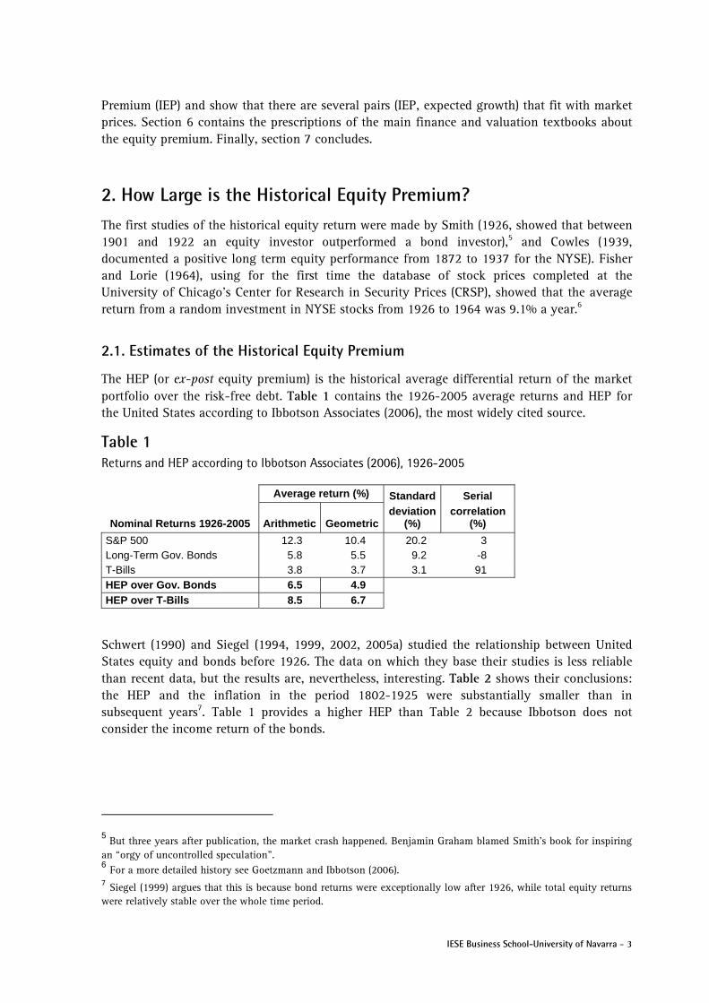
The HEP (or ex-post equity premium) is the historical average differential return of the market portfolio over the risk-free debt. Table 1 contains the 1926-2005 average returns and HEP for the United States according to Ibbotson Associates (2006), the most widely cited source.

Table 1 Returns and HEP according to Ibbotson Associates (2006), 1926-2005

Average return (%) Standard Serial

Nominal Returns 1926-2005 Arithmetic Geometric deviation

(%) correlation

(%)

S&P 500 12.3 10.4 20.2 3 Long-Term Gov. Bonds 5.8 5.5 9.2 -8 T-Bills 3.8 3.7 3.1 91 HEP over Gov. Bonds 6.5 4.9 HEP over T-Bills 8.5 6.7

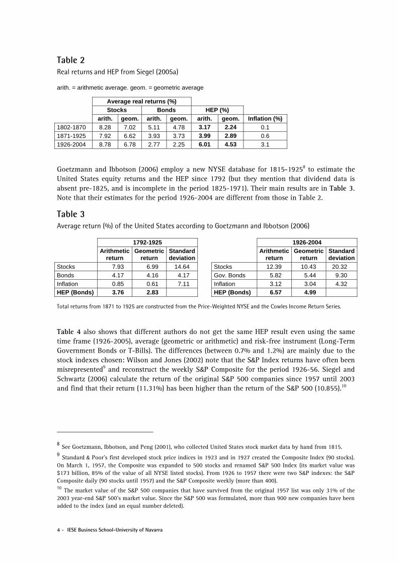
Schwert (1990) and Siegel (1994, 1999, 2002, 2005a) studied the relationship between United States equity and bonds before 1926. The data on which they base their studies is less reliable than recent data, but the results are, nevertheless, interesting. Table 2 shows their conclusions: the HEP and the inflation in the period 1802-1925 were substantially smaller than in subsequent years7. Table 1 provides a higher HEP than Table 2 because Ibbotson does not consider the income return of the bonds.

5 But three years after publication, the market crash happened. Benjamin Graham blamed Smith's book for inspiring an “orgy of uncontrolled speculation”. 6 For a more detailed history see Goetzmann and Ibbotson (2006). 7 Siegel (1999) argues that this is because bond returns were exceptionally low after 1926, while total equity returns were relatively stable over the whole time period.


Table 2 Real returns and HEP from Siegel (2005a)

arith. = arithmetic average. geom. = geometric average

Average real returns (%) Stocks Bonds HEP (%) arith. geom. arith. geom. arith. geom. Inflation (%)

1802-1870 8.28 7.02 5.11 4.78 3.17 2.24 0.1 1871-1925 7.92 6.62 3.93 3.73 3.99 2.89 0.6 1926-2004 8.78 6.78 2.77 2.25 6.01 4.53 3.1

Goetzmann and Ibbotson (2006) employ a new NYSE database for 1815-19258 to estimate the United States equity returns and the HEP since 1792 (but they mention that dividend data is absent pre-1825, and is incomplete in the period 1825-1971). Their main results are in Table 3. Note that their estimates for the period 1926-2004 are different from those in Table 2.

Table 3 Average return (%) of the United States according to Goetzmann and Ibbotson (2006)

1792-1925 1926-2004

Arithmetic

return Geometric

return Standard deviation

Arithmetic return

Geometric return

Standard deviation

Stocks 7.93 6.99 14.64 Stocks 12.39 10.43 20.32 Bonds 4.17 4.16 4.17 Gov. Bonds 5.82 5.44 9.30 Inflation 0.85 0.61 7.11 Inflation 3.12 3.04 4.32 HEP (Bonds) 3.76 2.83 HEP (Bonds) 6.57 4.99

Total returns from 1871 to 1925 are constructed from the Price-Weighted NYSE and the Cowles Income Return Series.

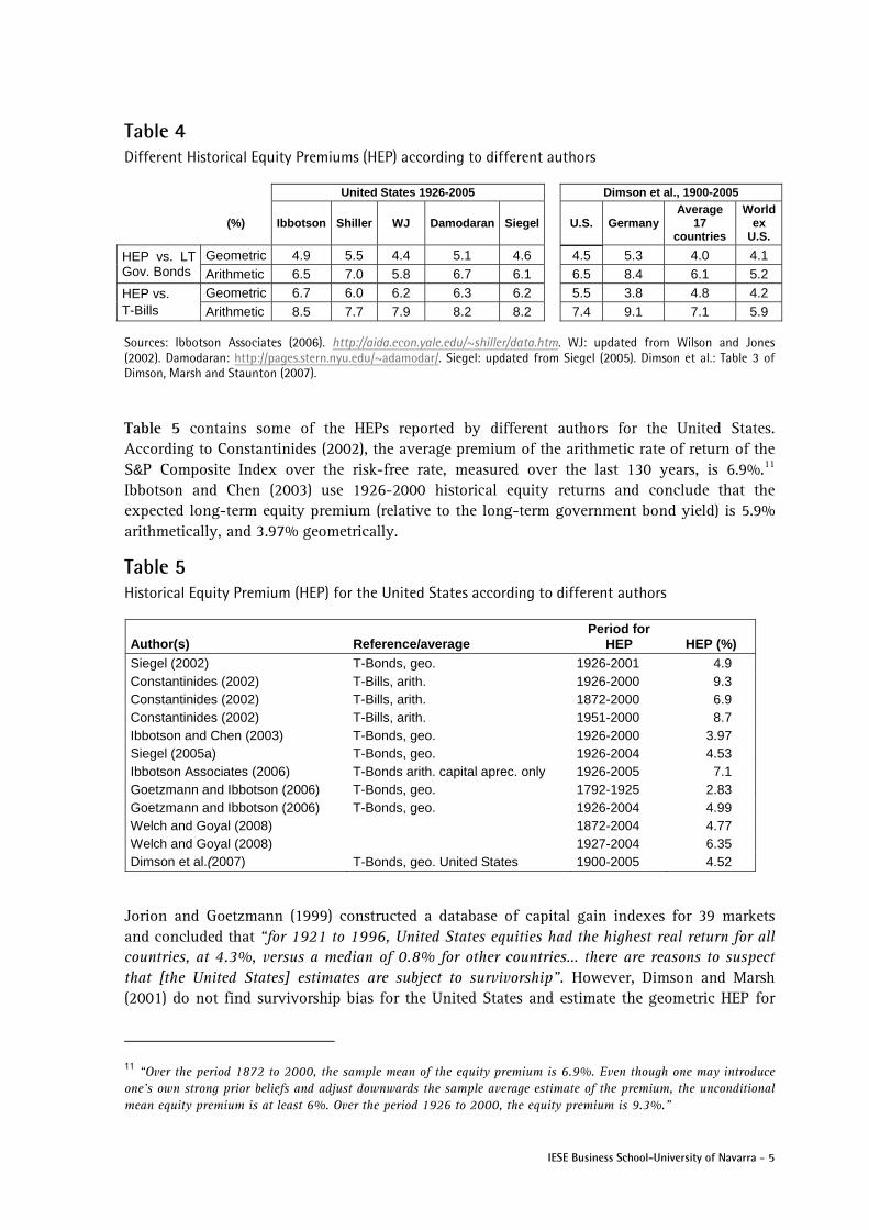
Table 4 also shows that different authors do not get the same HEP result even using the same time frame (1926-2005), average (geometric or arithmetic) and risk-free instrument (Long-Term Government Bonds or T-Bills). The differences (between 0.7% and 1.2%) are mainly due to the stock indexes chosen: Wilson and Jones (2002) note that the S&P Index returns have often been misrepresented9 and reconstruct the weekly S&P Composite for the period 1926-56. Siegel and Schwartz (2006) calculate the return of the original S&P 500 companies since 1957 until 2003 and find that their return (11.31%) has been higher than the return of the S&P 500 (10.855).10

8 See Goetzmann, Ibbotson, and Peng (2001), who collected United States stock market data by hand from 1815. 9 Standard & Poor's first developed stock price indices in 1923 and in 1927 created the Composite Index (90 stocks). On March 1, 1957, the Composite was expanded to 500 stocks and renamed S&P 500 Index (its market value was $173 billion, 85% of the value of all NYSE listed stocks). From 1926 to 1957 there were two S&P indexes: the S&P Composite daily (90 stocks until 1957) and the S&P Composite weekly (more than 400). 10 The market value of the S&P 500 companies that have survived from the original 1957 list was only 31% of the 2003 year-end S&P 500's market value. Since the S&P 500 was formulated, more than 900 new companies have been added to the index (and an equal number deleted).


Table 4 Different Historical Equity Premiums (HEP) according to different authors

United States 1926-2005 Dimson et al., 1900-2005

(%) Ibbotson Shiller WJ Damodaran Siegel U.S. Germany Average

17 countries

World ex

U.S.

Geometric 4.9 5.5 4.4 5.1 4.6 4.5 5.3 4.0 4.1 HEP vs. LT Gov. Bonds Arithmetic 6.5 7.0 5.8 6.7 6.1 6.5 8.4 6.1 5.2

Geometric 6.7 6.0 6.2 6.3 6.2 5.5 3.8 4.8 4.2 HEP vs. T-Bills Arithmetic 8.5 7.7 7.9 8.2 8.2 7.4 9.1 7.1 5.9

Sources: Ibbotson Associates (2006). http://aida.econ.yale.edu/~shiller/data.htm. WJ: updated from Wilson and Jones (2002). Damodaran: http://pages.stern.nyu.edu/~adamodar/. Siegel: updated from Siegel (2005). Dimson et al.: Table 3 of Dimson, Marsh and Staunton (2007).

Table 5 contains some of the HEPs reported by different authors for the United States. According to Constantinides (2002), the average premium of the arithmetic rate of return of the S&P Composite Index over the risk-free rate, measured over the last 130 years, is 6.9%.11 Ibbotson and Chen (2003) use 1926-2000 historical equity returns and conclude that the expected long-term equity premium (relative to the long-term government bond yield) is 5.9% arithmetically, and 3.97% geometrically.

Table 5 Historical Equity Premium (HEP) for the United States according to different authors

Author(s) Reference/average Period for

HEP HEP (%) Siegel (2002) T-Bonds, geo. 1926-2001 4.9 Constantinides (2002) T-Bills, arith. 1926-2000 9.3 Constantinides (2002) T-Bills, arith. 1872-2000 6.9 Constantinides (2002) T-Bills, arith. 1951-2000 8.7 Ibbotson and Chen (2003) T-Bonds, geo. 1926-2000 3.97 Siegel (2005a) T-Bonds, geo. 1926-2004 4.53 Ibbotson Associates (2006) T-Bonds arith. capital aprec. only 1926-2005 7.1 Goetzmann and Ibbotson (2006) T-Bonds, geo. 1792-1925 2.83 Goetzmann and Ibbotson (2006) T-Bonds, geo. 1926-2004 4.99 Welch and Goyal (2008) 1872-2004 4.77 Welch and Goyal (2008) 1927-2004 6.35 Dimson et al.(2007) T-Bonds, geo. United States 1900-2005 4.52

Jorion and Goetzmann (1999) constructed a database of capital gain indexes for 39 markets and concluded that “for 1921 to 1996, United States equities had the highest real return for all countries, at 4.3%, versus a median of 0.8% for other countries… there are reasons to suspect that [the United States] estimates are subject to survivorship”. However, Dimson and Marsh (2001) do not find survivorship bias for the United States and estimate the geometric HEP for

11 “Over the period 1872 to 2000, the sample mean of the equity premium is 6.9%. Even though one may introduce one’s own strong prior beliefs and adjust downwards the sample average estimate of the premium, the unconditional mean equity premium is at least 6%. Over the period 1926 to 2000, the equity premium is 9.3%.”


1955-1999 of United States, United Kingdom, Germany and Japan in 6.2%, 6.2%, 6.3% and 7.0%.

Dimson et al. (2002) show that the HEP was generally higher for the second half of the 20th century: the World had 4.7% in the first half, compared to 6.2% in the second half. The estimates of Dimson et al. (2007) (see Table 4) use data of 105 years but, as the authors point out, “virtually all of the 16 countries experienced trading breaks… often in wartime”: World War I, World War II, Spanish Civil War… They claim that “we were able to bridge these gaps,” but this assertion is questionable.12 Brailsford et al. (2008) also document concerns about data quality in Australia prior to 1958.

2.2. A Closer Look at the Historical Data

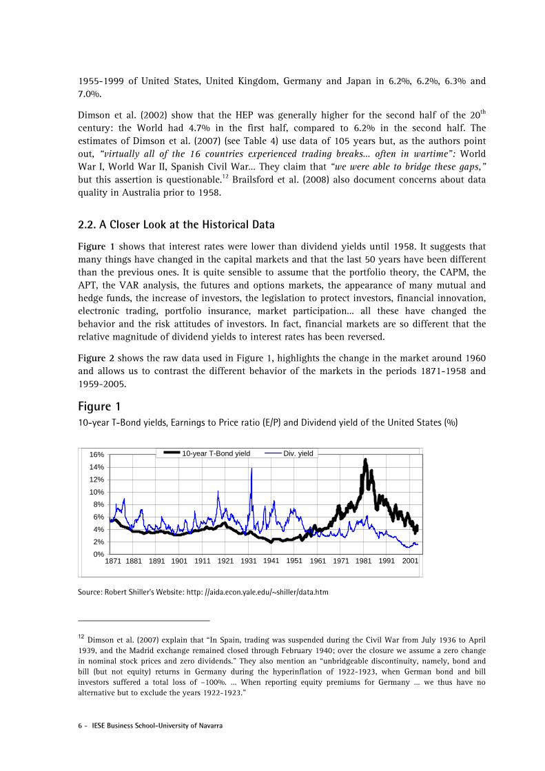
Figure 1 shows that interest rates were lower than dividend yields until 1958. It suggests that many things have changed in the capital markets and that the last 50 years have been different than the previous ones. It is quite sensible to assume that the portfolio theory, the CAPM, the APT, the VAR analysis, the futures and options markets, the appearance of many mutual and hedge funds, the increase of investors, the legislation to protect investors, financial innovation, electronic trading, portfolio insurance, market participation… all these have changed the behavior and the risk attitudes of investors. In fact, financial markets are so different that the relative magnitude of dividend yields to interest rates has been reversed.

Figure 2 shows the raw data used in Figure 1, highlights the change in the market around 1960 and allows us to contrast the different behavior of the markets in the periods 1871-1958 and 1959-2005.

Figure 1 10-year T-Bond yields, Earnings to Price ratio (E/P) and Dividend yield of the United States (%)

Source: Robert Shiller’s Website: http: //aida.econ.yale.edu/~shiller/data.htm

12 Dimson et al. (2007) explain that “In Spain, trading was suspended during the Civil War from July 1936 to April 1939, and the Madrid exchange remained closed through February 1940; over the closure we assume a zero change in nominal stock prices and zero dividends.” They also mention an “unbridgeable discontinuity, namely, bond and bill (but not equity) returns in Germany during the hyperinflation of 1922-1923, when German bond and bill investors suffered a total loss of –100%. … When reporting equity premiums for Germany … we thus have no alternative but to exclude the years 1922-1923.”

0%

2%

4%

6%

8%

10%

12%

14%

16%

1871 1881 1891 1901 1911 1921 1931 1941 1951 1961 1971 1981 1991 2001

10-year T-Bond yield Div. yield


Figure 2 (Dividend yield – RF) versus RF (yield on Government long-term bonds)

Source of the raw data: Robert Shiller’s Website: http://aida.econ.yale.edu/~shiller/data.htm

Figure 3 shows the evolution of the HEP for the United States. The HEP since 1926 has been always higher than 6%, while the HEP calculated with the data of the last 20 years has varied over time between 0 and 16%.

Figure 3 HEP (Historical Equity Premium) of the United States Market. Geometric average of the differential return of the S&P 500 and the T-Bills

Source of the data: Ibbotson and Datastream.

Harvey and Siddique (2000) show that the equity premium is non-normally distributed, exhibiting excess kurtosis and significant negative skewness.

3. Some Attempts to Explain the Equity Premium Puzzle

The equity premium puzzle (the HEP is greater than theory predicts) has lead to an extensive research effort in both macroeconomics and finance. Over the last 23 years, researchers have tried to resolve the puzzle by generalizing and adapting some assumptions of the Mehra-Prescott (1985) model, but there is no solution generally accepted by the economics profession. Some of the adapted assumptions include:

-10%

-5%

0%

5%

10%

2% 4% 6% 8% 10% 12% 14% 16%

RF

Div

. yie

ld -

RF

1959-2006

-10%

-5%

0%

5%

10%

2% 4% 6% 8% 10% 12% 14% 16%

RF

Div

. yie

ld -

RF

1871-1958

0%

2%

4%

6%

8%

10%

12%

14%

16%

1-50 1-60 1-70 1-80 1-90 1-00 1-10

His

toric

al E

quity

Pre

miu

m

geo HEP since 1926

geo HEP 20 years

geo. HEP since 1962

geo. HEP 20 years


• Alternative assumptions about preferences (state separability, leisure, precautionary savings) or generalizations to state-dependent utility functions: Abel, 1990; Constantinides, 1990; Epstein and Zin, 1991; Bakshi and Chen, 1996; Campbell and Cochrane, 1999 and Barberis et al. 2001.

• Narrow framing:13 Benartzi and Thaler, 1995; Barberis and Huang, 2006.

• Probability distributions that admit disastrous events such as fear of catastrophic consumption drops: Rietz,1988; Mehra and Prescott, 1988; Barro, 2006.14

• Bayesian updating of unknown structural parameters: Weitzman (2007),15 and Gollier, 2007.

• Survivorship bias: Brown et al., 1995.

• Liquidity premium: Bansal and Coleman, 1996.

• Changes in taxes and regulation: McGrattan and Prescott, 2005.16

• The presence of uninsurable income shocks or incomplete markets: Mankiw, 1986; Constantinides and Duffie, 1996; Heaton and Lucas, 1996, 1997; Storesletten et al., 1999.

• Relative volatility of stocks and bonds: Asness, 2000.

• Limited stock market participation and limited diversification: Saito, 1995; Basak and Cuocco, 1998; Heaton and Lucas, 2000;17 Vissing-Jorgensen, 2002; Gomes and Michaelides, 2005.

• Distinguishing between the cash flows to equity and aggregate consumption: Brennan and Xia, 2001.

• Transaction costs in the form of borrowing constraints: Constantinides et al., 2002.

• Other market imperfections: Aiyagari and Gertler, 1991; Alvarez and Jermann, 2000.

13 Narrow framing is the phenomenon documented in experimental settings whereby, when people are offered a new gamble, they sometimes evaluate it in isolation, separately from their other risks. 14 Rietz (1988) and Barro (2006) suggest that low-probability disasters, such as a large “crash” in consumption or an economic depression with partial default by the government on its borrowing may justify a large equity premium. However, Mehra and Prescott (1988) challenge Rietz to identify such catastrophic events and estimate their probabilities. 15 Weitzman (2007) and Gollier (2007) acknowledge the presence of parameter uncertainty: they allow for several plausible scenarios for future growth and show that, in such an environment, rates should in effect be lower the greater the maturity. However, Granger (2007) claims that Weitzman uses an unrealistically tight distribution for return deviations. 16 McGrattan and Prescott (2005) argue that the 1960-2001 HEP is mainly due to changes in taxes and regulatory policy during this period, and they affirm that “Allowing for heterogeneous individuals will also help quantify the effects of increased market participation and diversification that has occurred in the past two decades”. 17 Heaton and Lucas (2000), using an overlapping generations model, concluded that the increases in participation of the past two decades are unlikely to cause a significant reduction in the EEP, but that improved portfolio diversification might explain a fall in the EEP of several percentage points.


• Disentangling the equity premium into its cash flow and discounting components: Bakshi and Chen, 2006.

• Measurement errors and poor consumption growth proxies: Breeden et al., 1989; Mankiw and Zeldes, 1991; Ferson and Harvey, 1992; Ait-Sahalia et al, 2006.

• Shifting volatility in the real economy: Lettau et al., 2008.18

There are several excellent surveys of this work, including Cochrane (1997), Mehra and Prescott (2003 and 2006), and Kocherlakota (1996), who admits that “the large equity premium is still largely a mystery to economists.”

Limited stock market participation can increase the REP by concentrating stock market risk on a subset of the population. To understand why limited participation may have quantitative significance for the REP, it is useful to review basic facts about the distribution of wealth, and its dynamics over time. Mishel et al. (2006) document that wealth and stock holdings in the United States remain highly concentrated in dollar terms: in 2004, the wealthiest 10% held 78.8% of the stocks (84% in 1989), and the wealthiest 20% held over 90% of all stocks. Only 48.6% of United States households held stocks in 2004 (31.7% in 1989) and only 34.9% (22.6% in 1989) held stock worth more than $5,000. Of this 34.9%, only 13.5% had direct holdings. Mankiw and Zeldes (1991) reported that 72.4% of the 2998 families in their survey held no stocks at all. Among the families that held more than $100,000 in liquid assets, only 48% held stock. The covariance of stock returns and consumption of the families that hold stocks is triple that of no stockholders and it helps to explain part of the puzzle.

Brennan (2004) highlights the “democratization of equity Investment:” between 1989 and 2000, “while bond funds roughly tripled, equity funds went up by a factor of over 14!... the share of corporate equity held by mutual funds rose from 6.6% in 1990 to 18.3% in 2000.”

Abel (1991) hoped that “incorporating differences among investors or more general attitudes toward risk can explain the various statistical properties of asset returns.” Bakshi and Chen (1994) noted an increase in risk premiums as investors aged. Levy and Levy (1996) mentioned that the introduction of a small degree of diversity in expectations changed the dynamics of their model and produced more realistic results. Constantinides and Duffie (1996) introduced heterogeneity in the form of uninsurable, persistent and heteroscedastic labor income shocks.

It is interesting the quotation in Siegel and Thaler (1997): “no economic theorist has been completely successful in resolving the [equity premium] puzzle” ... but ... “most economists we know have a very high proportion of their retirement wealth invested in equities (as we do).”

4. Expected Equity Premium (EEP)

The Expected Equity Premium (EEP) is the answer to a question we all would like to answer accurately, namely: what incremental return do I expect from the market portfolio over the risk-free rate over the next years? The EEP is very important for investors who must decide how to allocate their portfolios to safe and risky assets. Some relevant questions about the EEP

18 They attribute the lower equity risk premiums of the 1990s to reduced volatility in real economic variables including employment, consumption and GDP growth.


are: Is its distribution objective and stationary? Does EEP vary over time? Is EEP ever negative? Does the market have an EEP?

Numerous papers and books assert that there must be an EEP common to all investors (to the representative investor) and identify the EEP with the REP. However, investors do not share “homogeneous expectations”19 and most equity investors do not hold the market portfolio but, rather, a subgroup of stocks. Heterogeneous investors do not hold the same portfolio of risky assets; in fact, no investor must hold the market portfolio to clear the market.

Several authors consider that the equity premium is a stationary process, and claim that the HEP is an unbiased estimate of the EEP (unconditional mean equity premium). For example, Mehra and Prescott (2003) state that “…over the long horizon the equity premium is likely to be similar to what it has been in the past”.20 However, the HEP changes over time, and it is not clear why capital market data from the 19th century or from the first half of the 20th century may be useful in estimating expected returns in the 21st century. As Shiller (2000) points out, “the future will not necessarily be like the past.” Booth (1999) concludes that the HEP is not a good estimator of the EEP and estimates the latter at 200 basis points smaller than the HEP.21 Mayfield (2004) suggest that a structural shift in the process governing the volatility of market returns after the 1930s resulted in a decrease in the expected level of market risk, and concluded that EEP = HEP – 2.4% = 5.9% over the yield on T-bills (4.1% over yields on T-bonds).

Survivorship bias22 was identified by Brown et al. (1995) as one of the main reasons why the results based on historical analyses can be too optimistic. They pointed out that the observed return, conditioned on survival (HEP), can overstate the unconditional expected return (EEP). However, Li and Xu (2002) show that the survival bias fails to explain the equity premium puzzle: “To have high survival bias, the probability of market survival over the long run has to be extremely small, which seems to be inconsistent with existing historical evidence.”

Pastor and Stambaugh (2001) present a framework allowing for structural breaks in the risk premium over time and estimate that the EEP fluctuated between 4% and 6% over the period from 1834 to 1999 and had the sharpest drop in the last decade of the 20th century. Using extra information from return volatility and prices, they narrow the confidence interval of their estimation (two standard deviations) to plus or minus 280 basis points around 4.8%.

Constantinides (2002) draws a sharp distinction between conditional short-term forecasts of the mean equity premium and estimates of the unconditional mean. He says that the conditional EEPs at the end of the 20th century and the beginning of the 21st are substantially lower than the estimates of the unconditional EEP (7%). But he concludes that “the low conditional

19 Brennan (2004) also admits that “different classes of investor may have different expectations about the prospective returns on equities which imply different assessments of the risk premium.” 20 In the 1970’s, the efficient market hypothesis was interpreted to mean that the true equity premium was a constant and was associated with the use of HEP to forecast EEP. 21 He also points out that the nominal equity return did not follow a random walk and that the volatility of the bonds increased significantly over the last 20 years. 22 “Survivorship” or “survival” bias applies not only to the stocks within the market (the fact that databases contain data on companies listed today, but they tend not to have data on companies that went bankrupt or filed for bankruptcy protection in the past), but also for the markets themselves (“US market’s remarkable success over the last century is typical neither of other countries nor of the future for US stocks,” Dimson et al., 2004).


forecasts do not necessarily lessen the burden on economic theory to explain the large sample average of the equity return and premium over the past 130 years.”

Dimson et al. (2003) conclude that the geometric EEP for the world’s major markets should be 3% (5% arithmetic). Dimson et al. (2007) admit that “we cannot know today’s consensus expectation for the equity premium”, but they affirm that “investors expect an equity premium (relative to bills) of around 3-3½% on a geometric mean basis,” substantially lower than the HEP found in their own study.

4.1. Surveys

A direct way to obtain an expectation of the equity premium is to carry out a survey of analysts or investors, although Ilmanen (2003) argues that surveys tend to be optimistic: “survey-based expected returns may tell us more about hoped-for returns than about required returns.” Shiller23 publishes and updates an index of investor sentiment since the crash of 1987. While neither survey provides a direct measure of the equity risk premium, they yield a broad measure of where investors expect stock prices to go in the near future. The 2004 survey of the Securities Industry Association (SIA) found that the median EEP of 1500 United States investors was about 8.3%. Merrill Lynch surveys more than 300 institutional investors globally in July 2008: the average EEP was 3.5%. Goldman Sachs (O'Neill et al., 2002) conducted a survey of its global clients in July 2002 and the average long-run EEP was 3.9%, with most responses between 3.5% and 4.5%. The magazine Pensions and Investments (12-1-1998) carried out a survey among professionals working for institutional investors and the average EEP was 3%.

Graham and Harvey (2007) indicate that United States CFOs reduced their average EEP from 4.65% in September 2000 to 2.93% by September 2006. In the 2008 survey, they report an average EEP of 3.80%, ranging from 3.1% to 11.5% at the tenth percentile at each end of the spectrum. They show that average EEP changes through time.

Welch (2000) performed two surveys with finance professors in 1997 and 1998, asking them what they thought the EEP was over the next 30 years. He obtained 226 replies, ranging from 1% to 15%, with an average arithmetic EEP of 7% above T-Bonds.24 Welch (2001) presented the results of a survey conducted in August 2001 of 510 finance and economics professors, and the consensus for the 30-year arithmetic EEP was 5.5%, much lower than just three years earlier. Damodaran (2008) points out that “the risk premiums in academic surveys indicate how far removed most academics are from the real world of valuation and corporate finance and how much of their own thinking is framed by the historical risk premiums... The risk premiums that are presented in classroom settings are not only much higher than the risk premiums in practice but also contradict other academic research.”

23 See http://icf.som.yale.edu/Confidence.Index 24 At that time, the most recent Ibbotson Associates Yearbook was the 1998 edition, with an arithmetic HEP versus T-bills of 8.9% (1926-1997).


4.2. Regressions

Attempts to predict the equity premium typically look for some independent lagged predictors (X) on the equity premium: Equity Premiumt = a + b ·Xt-1 + εt

Many predictors have been explored in the literature. Some examples are:

• Dividend yield: Ball, 1978; Rozeff, 1984; Campbell, 1987; Campbell and Shiller, 1988; Fama and French, 1988; Hodrick, 1992; Campbell and Viceira, 2002; Campbell and Yogo, 2006; Lewellen, 2004, and Menzly et al., 2004. Cochrane, 1997 has a good survey of the dividend yield prediction literature.

• Short term interest rate: Hodrick, 1992.

• Earnings price and payout ratio: Campbell and Shiller, 1988; Lamont, 1998, and Ritter 2005.

• Term spread and default spread: Avramov, 2002; Campbell, 1987; Fama and French, 1989, and Keim and Stambaugh, 1986.

• Inflation rate (money illusion): Fama and Schwert, 1977; Fama, 1981; Campbell and Vuolteenaho, 2004, and Cohen et al., 2005.25

• Interest rate and dividend related variables: Ang and Bekaert, 2007.

• Book-to-market ratio: Kothari and Shanken, 1997.

• Value of high and low-beta stocks: Polk et al., 2006.26

• Consumption and wealth: Lettau and Ludvigson, 2001.

• Aggregate financing activity: Baker and Wurgler, 2000, and Boudoukh et al., 2007.

Wachter and Warusawitharana (2007) claim that the predictability increases in a Bayesian setting that includes uncertainty about both the existence and strength of predictability.

However, Welch and Goyal (2008) argue that the historical mean has done as well at forecasting the expected equity premium as any of the more complex empirical models found in the literature. They used most of the mentioned predictors and could not identify one that would have been robust for forecasting the equity premium and, after all their analysis, they recommended “assuming that the equity premium is ‘like it always has been’.” They also show

25 Modigliani and Cohn (1979) argued that low equity values of the late 1970s were the consequence of investors’ money illusion (inconsistent treatment of inflation): investors were using historical growth rates in earnings to forecast future earnings and current interest rates (that incorporate expectations of future inflation), to estimate discount rates. When inflation increases, investors would use high discount rates and low cash flows. Damodaran (2008) affirms that “it is not so much the level of inflation that determines equity risk premiums but uncertainty about that level.” 26 Polk et al. (2006) argue that if the CAPM holds, then a high equity premium implies low prices for stocks that have high betas. Therefore, value stocks should tend to have high betas. This was true from the 1930’s through the 1950’s, but in recent decades growth stocks had higher betas than value stocks. Polk et al. argue that this change in cross-sectional stock pricing reflects a decline in the equity premium.


that most of these models have not performed well for the last thirty years, are not stable, and are not useful for market-timing purposes.

But Campbell and Thompson (2008) claim that some variables (stock market valuation ratios, patterns in corporate finance, levels of short- and long-term interest rates, level of consumption in relation to wealth) are correlated with subsequent market returns and that empirical models, restricting their parameters in economically justified ways, yield out-of-sample forecasts that beat the historical mean. They explore the mapping from R2 statistics in predictive regressions to profits and welfare gains for market timers. “The basic lesson is that investors should be suspicious of predictive regressions with high R2 statistics, asking the old question ‘If you’re so smart, why aren’t you rich?’.”

Pesaran and Timmermann (1995) point out that economist have snooped data and methods in search of models that “seem to predict” the equity premium. Ferson et al. (2003) also conclude that “many of the regressions in the literature, based on individual predictor variables, may be spurious.”

4.3. Other Estimates of the Expected Equity Premium

Siegel (2002, page 124) concluded that “the future equity premium is likely to be in the range of 2 to 3%, about one-half the level that has prevailed over the past 20 years.”27 Siegel (2005a, page 172) affirms that “over the past 200 years, the equity risk premium has averaged about 3%”. Siegel (2005b) maintains that “although the future equity risk premium is apt to be lower than it has been historically, United States equity returns of 2-3% over bonds will still amply reward those who will tolerate the short-term risk of stocks.”

In the TIAA-CREF Investment Forum of June 2002, Ibbotson forecasted “less than 4% in excess of long-term bond yields”, and Campbell “1.5% to 2%.”

McGrattan and Prescott (2001) did not find corporate equity overvalued in 2000 and forecasted a small equity premium in the future. Arnott and Ryan (2001) and Arnott and Bernstein (2002) also claim that the expected equity premium is near zero. They base their conclusion on the low dividend yield and their low expectation of dividend growth.

27 Siegel also affirms that: “Although it may seem that stocks are riskier than long-term government bonds, this is not true. The safest investment in the long run (from the point of view of preserving the investor’s purchasing power) has been stocks, not Treasury bonds.”


Table 6 Estimates of the EEP (Expected Equity Premium) according to different authors

Authors Conclusion about EEP Note

Surveys Pensions and Investments (1998) 3% Institutional investors Graham and Harvey (2000) 4.65% CFOs Welch (2000) 7% arithmetically, 5.2% geometrically Finance professors Welch (2001) 5.5% arithmetically, 4.7% geometrically Finance professors O'Neill, Wilson and Masih (2002) 3.9% Global clients Goldman Graham and Harvey (2007) 2.93% CFOs

Other publications Booth (1999) EEP = HEP - 2% Pastor and Stambaugh (2001) 4 -6% McGrattan and Prescott (2001) near zero Arnott and Ryan (2001) near zero Arnott and Bernstein (2002) near zero Siegel (2002, 2005b) 2 - 3% Ibbotson (2002) < 4% Campbell (2002) 1.5 - 2% Mayfield (2004) EEP = HEP - 2.4%= 5.9% + T-Bill Bostock (2004) 0.6 – 1.8% Welch and Goyal (2008) EEP = HEP Dimson, Marsh and Staunton (2007) 3 - 3.5% Grabowski (2006) 3.5 – 6% Maheu and McCurdy (2008) 4.02% and 5.1%. Ibbotson Associates (2006) EEP = HEP = 7.1% Welch (2007) EEP = 7.9%

Bostock (2004) concludes that, according to historical average data, equities should offer a risk premium over government bonds between 0.6% and 1.8%.

Grabowski (2006) concludes that “after considering the evidence, any reasonable long-term estimate of the normal EEP as of 2006 should be in the range of 3.5% to 6%.”

Maheu and McCurdy (2008) claim that the United States Market had “three major structural breaks (1929, 1940 and 1969), and possibly a more recent structural break in the late 1990s,” and suggest an EEP in 2004 between 4.02% and 5.1%.

Welch (2007) estimates the EEP for the period 1962-2007 in 7.9%.

The wide range of the estimates of the EEP may lead to a conclusion similar to that of Brealey et al. (2005): “Out of this debate only one firm conclusion emerges: Do not trust anyone who claims to know what returns investors expect.”

5. Required and Implied Equity Premium The Required Equity Premium (REP) of an investor is the incremental return that the investor requires, over the risk-free rate, for investing in a diversified portfolio of shares. It is a crucial parameter in valuation and capital budgeting because the REP is the key to determining the company’s required return to equity and the required return to any investment project.


However, the HEP is misleading for predicting the REP: if there was a reduction in the REP, this fall in the discount rate would lead to re-pricing of stocks, thus adding to the magnitude of HEP. The HEP, then, would overstate the REP.

The IEP is the implicit REP used in the valuation of a stock (or a market index) that matches the current market value with an estimate of the future cash flows to equity. The IEP is also called the ex ante equity premium. However, the existence of a unique IEP implies either that the equity market can be explained with a representative consumer, or that all investors have at any moment the same expectations about future cash flows and use the same discount rate to value each company.

Two models are widely used to calculate the IEP: the Gordon (1962) model (constant dividend growth model) and the residual income (or abnormal return) model. According to the Gordon (1962) model, the current price per share (P0) is the present value of expected dividends discounted at the required rate of return (k). If d1 is the dividend per share expected to be received at time 1, and g the expected long term growth rate in dividends per share,28

P0 = d1 / (k - g), which implies: k = d1/P0 + g, and IEP = d1/P0 + g - RF (1)

The abnormal return method is another version of the Gordon (1962) model when the “clean surplus” relation holds (dt = et – (bvt – bvt-1); d being the dividends per share, e the earnings per share and bv the book value per share):

P0 = bv0 + (e1 – k bv0) / (k - g), which implies: k = e1/P0 + g (1 - bv0/ P0)29 (2)

Jagannathan et al. (2000) use the Gordon model, assume that dividends will growth as fast as GNP, and reach an average estimate of 3.04% for 1926-1999. However, they mention that “the premium averaged about 7% during 1926-1970 and only about 0.7% after that.” They also review Welch (2000) and point out that “apparently, finance professors do not expect the equity premium to shrink”.

Glassman and Hassett (2000) calculated in their book Dow 36,000 that the REP for the United States in 1999 was 3%, and argued that stocks should not carry any risk premium at all, and that stock prices will rise dramatically further once investors come to realize this fact.30

O'Hanlon and Steele (2000) calculated the REP using accounting figures and got estimates between 4 and 6%.

Harris and Marston (2001), using the dividend discount model and estimations of the financial analysts about long-run growth in earnings, estimated an IEP of 7.14% for the S&P 500 above T-Bonds. They also claim that IEP moves inversely with government rates, which is hard to believe.

Claus and Thomas (2001) calculated the equity premium using the Gordon model and the residual income model, assuming that g is the consensus of the analysts’ earnings growth forecasts for the next five years and that the dividend payout will be 50%. They also assumed

28 “Dividends per share”, refers to equity cash flow per share: dividends, repurchases and all expected cash for the shareholders. 29 In a growing perpetuity, d1 = e1 – g bv0. The equivalence of the two models may be seen in Fernández (2005). 30 Not to be outdone, Kadlec and Acampora (1999) gave their book the title, “Dow 100,000: Fact or Fiction?”.


that the residual earnings growth after year 5 will be the current 10-year risk-free rate less 3%. With data from 1985 to 1998, they recommended using a REP of about 3% for the United States.

Fama and French (2002), using the dividend discount model, estimated the IEP for the period 1951-2000 between 2.55% and 4.32%. For the period 1872-1950, they estimated an IEP of 4.17%. They claimed that “the unconditional EEP of the last 50 years is probably far below the realized premium”.31 Vivian (2005) replicated Fama and French (2002) for the United Kindgom, obtained similar results and concluded that the REP declined in the later part of the 20th century.

Goedhart et al. (2002) used the dividend discount model (considering also share repurchases), with GDP growth as a proxy for expected earnings growth and with the average inflation rate of the last five years as a proxy for expected inflation. They report an IEP of 5% in 1962-1979 and 3.6% in 1990-2000 for the United States. They conclude that “the implied equity risk premium is around 3.5% to 4% for the United States and the United Kingdom markets.”

Ritter and Warr (2002) claimed that in 1979-1997, the IEP declined from +12% to -4%, and Ritter (2002) claims that it was only 0.7%.

Easton et al. (2002) used the residual income model with IBES data for expected growth,32 and estimated an average IEP of 5.3% over the years 1981-1998.

Harris et al. (2003) estimated discount rates for several companies using the dividend discount model and assuming that g was equal to the consensus of the analysts’ growth of dividends per share forecasts. They found an IEP of 7.3% (if betas calculated with a domestic index) and 9.7% (when betas calculated with a world index).

Faugere and Erlach (2006) claimed that the equity premium tracks the value of a put option on the S&P 500. However, their conclusion is not very helpful because they admit that both 3.5% and 8.1% are reasonable estimates of the equity premium.

Donaldson et al. (2007) simulate the distribution from which interest rates, dividend growth rates, and equity premia are drawn and claim that IEP is between 3 and 4%.

31 Fama and French (1992) report that, in the period 1941-1990, an equally weighted index outperformed the value weighted (average monthly returns of 1.12% and 0.93%) in the whole period and in most sub sample periods. 32 Although Chan et al. (2003) report that “IBES forecasts are too optimistic and have low predictive power for long-term growth.”


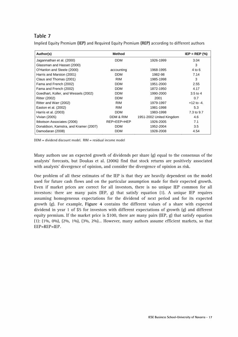
Table 7 Implied Equity Premium (IEP) and Required Equity Premium (REP) according to different authors

Author(s) Method IEP = REP (%)

Jagannathan et al. (2000) DDM 1926-1999 3.04 Glassman and Hasset (2000) 3 O'Hanlon and Steele (2000) accounting 1968-1995 4 to 6 Harris and Marston (2001) DDM 1982-98 7.14 Claus and Thomas (2001) RIM 1985-1998 3 Fama and French (2002) DDM 1951-2000 2.55 Fama and French (2002) DDM 1872-1950 4.17 Goedhart, Koller, and Wessels (2002) DDM 1990-2000 3.5 to 4 Ritter (2002) DDM 2001 0.7 Ritter and Warr (2002) RIM 1979-1997 +12 to -4. Easton et al. (2002) RIM 1981-1998 5.3 Harris et al. (2003) DDM 1983-1998 7.3 to 9.7 Vivian (2005) DDM & RIM 1951-2002 United Kingdom 4.6 Ibbotson Associates (2006) REP=EEP=HEP 1926-2005 7.1 Donaldson, Kamstra, and Kramer (2007) DDM 1952-2004 3.5 Damodaran (2008) DDM 1928-2008 4.54

DDM = dividend discount model. RIM = residual income model

Many authors use an expected growth of dividends per share (g) equal to the consensus of the analysts’ forecasts, but Doukas et al. (2006) find that stock returns are positively associated with analysts’ divergence of opinion, and consider the divergence of opinion as risk.

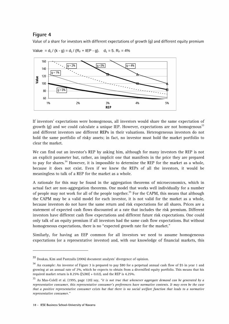
One problem of all these estimates of the IEP is that they are heavily dependent on the model used for future cash flows and on the particular assumption made for their expected growth. Even if market prices are correct for all investors, there is no unique IEP common for all investors: there are many pairs (IEP, g) that satisfy equation (1). A unique IEP requires assuming homogeneous expectations for the dividend of next period and for its expected growth (g). For example, Figure 4 contains the different values of a share with expected dividend in year 1 of $5 for investors with different expectations of growth (g) and different equity premium. If the market price is $100, there are many pairs (IEP, g) that satisfy equation (1): (1%, 0%), (2%, 1%), (3%, 2%)… However, many authors assume efficient markets, so that EEP=REP=IEP.


Figure 4 Value of a share for investors with different expectations of growth (g) and different equity premium

Value = d1 / (k - g) = d1 / (RF + IEP - g). d1 = 5. RF = 4%

If investors’ expectations were homogenous, all investors would share the same expectation of growth (g) and we could calculate a unique IEP. However, expectations are not homogenous33 and different investors use different REPs in their valuations. Heterogeneous investors do not hold the same portfolio of risky assets; in fact, no investor must hold the market portfolio to clear the market.

We can find out an investor’s REP by asking him, although for many investors the REP is not an explicit parameter but, rather, an implicit one that manifests in the price they are prepared to pay for shares.34 However, it is impossible to determine the REP for the market as a whole, because it does not exist. Even if we knew the REPs of all the investors, it would be meaningless to talk of a REP for the market as a whole.

A rationale for this may be found in the aggregation theorems of microeconomics, which in actual fact are non-aggregation theorems. One model that works well individually for a number of people may not work for all of the people together.35 For the CAPM, this means that although the CAPM may be a valid model for each investor, it is not valid for the market as a whole, because investors do not have the same return and risk expectations for all shares. Prices are a statement of expected cash flows discounted at a rate that includes the risk premium. Different investors have different cash flow expectations and different future risk expectations. One could only talk of an equity premium if all investors had the same cash flow expectations. But without homogeneous expectations, there is no “expected growth rate for the market.”

Similarly, for having an EEP common for all investors we need to assume homogeneous expectations (or a representative investor) and, with our knowledge of financial markets, this

33 Doukas, Kim and Pantzalis (2006) document analysts’ divergence of opinion. 34 An example: An investor of Figure 3 is prepared to pay $80 for a perpetual annual cash flow of $5 in year 1 and growing at an annual rate of 2%, which he expects to obtain from a diversified equity portfolio. This means that his required market return is 8.25% ([5/80] + 0.02), and the REP is 4.25%. 35 As Mas-Colell et al. (1995, page 120) say, “it is not true that whenever aggregate demand can be generated by a representative consumer, this representative consumer’s preferences have normative contents. It may even be the case that a positive representative consumer exists but that there is no social welfare function that leads to a normative representative consumer.”

60

80

100

120

140

160

1% 2% 3% 4% 5%REP

Valu

e

g = 0%

g = 1%

g = 2% g =3% g = 4%


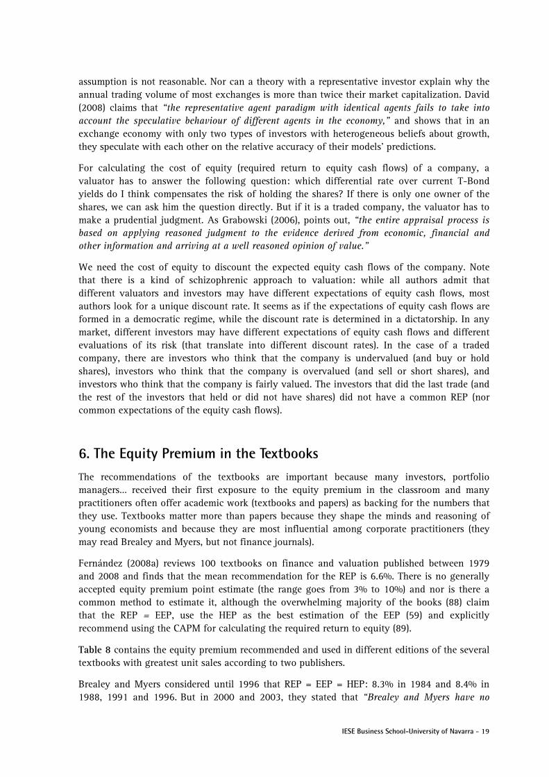
assumption is not reasonable. Nor can a theory with a representative investor explain why the annual trading volume of most exchanges is more than twice their market capitalization. David (2008) claims that “the representative agent paradigm with identical agents fails to take into account the speculative behaviour of different agents in the economy,” and shows that in an exchange economy with only two types of investors with heterogeneous beliefs about growth, they speculate with each other on the relative accuracy of their models’ predictions.

For calculating the cost of equity (required return to equity cash flows) of a company, a valuator has to answer the following question: which differential rate over current T-Bond yields do I think compensates the risk of holding the shares? If there is only one owner of the shares, we can ask him the question directly. But if it is a traded company, the valuator has to make a prudential judgment. As Grabowski (2006), points out, “the entire appraisal process is based on applying reasoned judgment to the evidence derived from economic, financial and other information and arriving at a well reasoned opinion of value.”

We need the cost of equity to discount the expected equity cash flows of the company. Note that there is a kind of schizophrenic approach to valuation: while all authors admit that different valuators and investors may have different expectations of equity cash flows, most authors look for a unique discount rate. It seems as if the expectations of equity cash flows are formed in a democratic regime, while the discount rate is determined in a dictatorship. In any market, different investors may have different expectations of equity cash flows and different evaluations of its risk (that translate into different discount rates). In the case of a traded company, there are investors who think that the company is undervalued (and buy or hold shares), investors who think that the company is overvalued (and sell or short shares), and investors who think that the company is fairly valued. The investors that did the last trade (and the rest of the investors that held or did not have shares) did not have a common REP (nor common expectations of the equity cash flows).

6. The Equity Premium in the Textbooks The recommendations of the textbooks are important because many investors, portfolio managers… received their first exposure to the equity premium in the classroom and many practitioners often offer academic work (textbooks and papers) as backing for the numbers that they use. Textbooks matter more than papers because they shape the minds and reasoning of young economists and because they are most influential among corporate practitioners (they may read Brealey and Myers, but not finance journals).

Fernández (2008a) reviews 100 textbooks on finance and valuation published between 1979 and 2008 and finds that the mean recommendation for the REP is 6.6%. There is no generally accepted equity premium point estimate (the range goes from 3% to 10%) and nor is there a common method to estimate it, although the overwhelming majority of the books (88) claim that the REP = EEP, use the HEP as the best estimation of the EEP (59) and explicitly recommend using the CAPM for calculating the required return to equity (89).

Table 8 contains the equity premium recommended and used in different editions of the several textbooks with greatest unit sales according to two publishers.

Brealey and Myers considered until 1996 that REP = EEP = HEP: 8.3% in 1984 and 8.4% in 1988, 1991 and 1996. But in 2000 and 2003, they stated that “Brealey and Myers have no


official position on the exact market risk premium, but we believe a range of 6 to 8.5% is reasonable for the United States.” In 2005, they increased that range to 5 to 8%.

Copeland et al. (1990 and 1995), authors of the McKinsey book on valuation, advised using a REP = HEP, which were 6% and 5.5% respectively. However, in 2000 they recommended 4.5-5% and in 2005 they used a REP of 4.8% that was the HEP reduced by a survivorship bias.36

Ross et al. recommended in all editions that REP = EEP = HEP: 8.5% (1988-96), 9.2% (1999), 9.5% (2002) and 8.4% (2005).

Bodie et al. (1993) used a REP = EEP = 6.5%. In 1996, they used a REP = EEP = HEP – 1% = 7.75%. In 2002, they used a REP = 6.5%, but in 2003 and 2004, they used different REPs: 8% and 5%.

Table 8 Equity premiums recommended and used in some textbooks

Author(s) of the Textbook Assumption Period for

HEP REP

recommended REP used Brealey and Myers 2nd edition. 1984 REP=EEP= arith HEP vs. T-Bills 1926-1981 8.3% 8.3% 3rd edition. 1988 REP=EEP= arith HEP vs. T-Bills 1926-1985 8.4% 8.4% 4th edition. 1991 REP=EEP= arith HEP vs. T-Bills 1926-1988 8.4% 8.4% 5th edition. 1996 REP=EEP= arith HEP vs. T-Bills 1926-1995 8.2 - 8.5% 8.0% 6th and 7th edition. 2000 and 2003 No official position 6.0 - 8.5% 8.0% 8th edition. 2005 (with Allen) No official position 5.0 - 8.5% 6-8.5%

Copeland, Koller, and Murrin (McKinsey) 1st edition. 1990 REP=EEP= geo HEP vs. T-Bonds 1926-1988 5 - 6% 6.0% 2nd ed. 1995 REP=EEP= geo HEP vs. T-Bonds 1926-1992 5 - 6% 5.5% 3rd ed. 2000 REP=EEP= arith HEP – 1.5-2% 1926-1998 4.5 - 5% 5.0% 4th ed. 2005. Goedhart, Koller, & Wessels REP=EEP= arith HEP – 1-2% 1903-2002 3.5 - 4.5% 4.8%

Ross, Westerfield, and Jaffe 2nd edition. 1988 REP=EEP= arith HEP vs. T-Bills 1926-1988 8.5% 8.5% 3rd edition. 1993 REP=EEP= arith HEP vs. T-Bills 1926-1993 8.5% 8.5% 4th edition. 1996 REP=EEP= arith HEP vs. T-Bills 1926-1994 8.5% 8.5% 5th edition. 1999 REP=EEP= arith HEP vs. T-Bills 1926-1997 9.2% 9.2% 6th edition. 2002 REP=EEP= arith HEP vs. T-Bills 1926-1999 9.5% 9.5% 7th edition. 2005 REP=EEP= arith HEP vs. T-Bills 1926-2002 8.4% 8.0% Bodie, Kane, and Marcus 2nd edition. 1993 REP=EEP 6.5% 6.5% 3rd edition. 1996 REP=EEP=arith HEP vs. T-Bills - 1% 7.75% 7.75% 5th edition. 2002 6.5% 6.5% 2003 REP=EEP= arith HEP vs. T-Bills 1926-2001 5%; 8% Damodaran 1994 Valuation. 1st ed. REP=EEP= geo HEP vs.T-Bonds 1926-1990 5.5% 5.5% 1996, 1997, 2001b, 2001c REP=EEP= geo HEP vs.T-Bonds 5.5% 5.5% 2001a average IEP 1970-2000 4.0% 4.0% 2002 REP=EEP= geo HEP vs.T-Bonds 1928-2000 5.51% 5.51% 2006 Valuation. 2nd ed. REP=EEP= geo HEP vs.T-Bonds 1928-2004 4.84% 4.0%

Bodie and Merton (2000) 8% Stowe et al. (2002) REP=EEP= geo HEP vs.T-Bonds 1926-2000 5.7% 5.7% Penman (2001, 2003) “No one knows what the REP is” 6.0% Bruner (2004) REP=EEP= geo HEP vs.T-Bonds 1926-2000 6% 6.0% Palepu, Healy, and Bernard (2004) REP=EEP= arith HEP vs.T-Bonds 1926-2002 7% 7.0% Arzac (2007) REP=IEP 5.08% 5.08%

36 In 1990 and 1995 they calculated the HEP using geometric averages (“because arithmetic averages are biased by the measurement period”), but in 2000 and 2005 they used arithmetic averages.


Damodaran recommended in 1994, 1996, 1997, 2001b, 2001c and 2002 REP = EEP = HEP = 5.5%.37 In 2001a and 2006, he used a REP = IEP = 4%.

Bodie and Merton (2000) used 8% for United States, while Stowe et al. (2002, Chartered Financial Analysts Program) used a REP = HEP = 5.7%.38

According to Penman (2001), “the market risk premium is a big guess… No one knows what the market risk premium is.” In 2003, he admitted that “estimates [of the equity premium] range, in texts and academic research, from 3.0% to 9.2%,” and he used 6%.

Bruner (2004) used a REP = HEP = 6%, Palepu et al. (2004) 7%, and Arzac (2007) used a REP of 4.36%; the IEP calculated using a Gordon equation.

Siegel (2002) concluded that “the EEP is likely to be in the range of 2 to 3%, about one-half the level that has prevailed over the past 20 years”.39 Siegel (2007) affirms that “the abnormally high HEP since 1926 is certainly not sustainable.”

According to Shapiro (2005, page 148) “an expected equity risk premium of 4 to 6% appears reasonable. In contrast, the historical equity risk premium of 7% appears to be too high for current conditions.” However, he uses different REPs in his examples: 5%, 7.5% and 8%.

Figure 5 collects the evolution of the Required Equity Premium (REP) used or recommended by the textbooks and by the academic papers mentioned in previous sections. The average of the recommendations is 6.3% in the textbooks and 4.2% in the papers. Looking at Figure 5 and at Table 8, it is quite obvious that there is not much consensus among finance authors regarding the equity premium: perhaps the conventional wisdom is not wisdom, but confusion. Why this is so?

Figure 5 Evolution of the Required and Expected Equity Premium used or recommended in the most important finance textbooks and academic papers

37 Damodaran (2001c, page 192): “we must confess that this is more for the sake of continuity with the previous version of the book and for purposes of saving a significant amount of reworking practice problems and solutions.” 38 They also mention the “bond yield plus risk premium method.” Under this approach, the cost of equity is equal to the “yield to maturity on the company´s long-term debt plus a typical risk premium of 3-4%, based on experience.” 39 Siegel also affirms that: “Although it may seem that stocks are riskier than long-term government bonds, this is not true. The safest investment in the long run (from the point of view of preserving the investor’s purchasing power) has been stocks, not Treasury bonds.”

Required and Expected Equity Premium

0%

1%

2%

3%

4%

5%

6%

7%

8%

9%

10%

1978

1980

1982

1984

1986

1988

1990

1992

1994

1996

1998

2000

2002

2004

2006

2008

Textbooks Papers


The REPs used to calculate the cost of equity in the teaching notes published by Harvard Business School have decreased over time. Until 1989 most teaching notes used REPs between 8 and 9%; in 1989, the REPs used were in the 6-9% range, and in 2000 6%. The REPs used in the teaching notes published by the Darden Business School over that period have been in the 5.4-6% range.

Ritter (2002) mentions the use of the HEP in textbooks as an estimate of the EEP as one of the "The Biggest Mistakes We Teach."

7. Conclusion Mehra and Prescott (1985) argued that, according to sensible asset pricing models, stocks should provide at most a 0.35% premium over bills. However, professors use in, class and in their textbooks, higher equity premia (average around 6%, range from 3 to 10%), investors use higher equity premia for valuing companies, and companies use higher equity premia (average around 6%) for evaluating their investment projects. The overall result is that equity prices are, on average, undervalued (and have been undervalued in the last decades) and, consequently, the measured ex-post equity premium (HEP) is also high.

If the additional returns beyond the risk-free rate demanded by equity investors (ex-ante risk premia) and used in financial asset pricing models have been high, it is not a surprise that the ex-post risk premia (calculated with historical data) have been also high. If most investors use historical data to estimate the required and the expected equity premium, the undervaluation and the high ex-post risk premium are self fulfilling prophecies.

The equity premium (also called market risk premium, equity risk premium, market premium and risk premium), is one of the most important, discussed but elusive parameters in finance. The term equity premium is used to designate four different concepts (although they are often mixed): Historical Equity Premium (HEP), Expected Equity Premium (EEP); Required Equity Premium (REP) and Implied Equity Premium (IEP).

It has been argued that, from an economic standpoint, we need to establish the primacy of the EEP, since it is what guides investors' decisions. However, the REP is more important for many important decisions; among others, valuations of projects and companies, acquisitions, and corporate investment decisions. The EEP is important only for the investors that hold the market portfolio.


References Abel, A.B. (1990), “Asset Prices under Habit Formation and Catching Up with the Joneses,”

American Economic Review, Vol. 80, No. 2 (May), pp. 38-42.

Abel, A.B. (1991), “The Equity Premium Puzzle,” Business Review (Federal Reserve Bank of Philadelphia), pp. 3-14.

Ait-Sahalia, Y., J. A. Parker, and M. Yogo (2004), “Luxury Goods and the Equity Premium,” Journal of Financ, 59, pp. 2959-3004.

Aiyagari, S.R. and M. Gertler (1991), “Asset Returns with Transactions Costs and Uninsured Individual Risk,” Journal of Monetary Economics, Vol. 27, No. 3 (June), pp. 311-331.

Alvarez, F. and U. Jermann (2000), “Efficiency, Equilibrium, and Asset Pricing with Risk of Default,, Econometrica, Vol. 68, No. 4 (July), pp. 775-797.

Ang, A. and G. Bekaert (2007), “Stock Return Predictability: Is It There?,” Review of Financial Studies, 20 (3), pp. 651-707.

Arnott, R. D. and R. J. Ryan (2001), “The Death of the Risk Premium,” Journal of Portfolio Management, Spring, pp. 61-74.

Arnott, R. D. and P. L. Bernstein (2002), “What Risk Premium is ‘Normal’?,” Financial Analysts Journal, Vol. 58, No. 2, pp. 64-84.

Arzac, E. R. (2007), “Valuation for Mergers, Buyouts, and Restructuring,” John Wiley & Sons Inc, 2nd ed.

Asness, C.S. (2000), “Stocks versus Bonds: Explaining the Equity Risk Premium,” Financial Analysts Journal, March/April, Vol. 56, No. 2, pp. 96-113.

Avramov, D. (2002), “Stock Return Predictability and Model Uncertainty,” Journal of Financial Economics (3), pp. 423-458.

Baker, M and J. Wurgler (2000), “The Equity Share in New Issues and Aggregate Stock Returns,” Journal of Finance, 55, 5, pp. 2219-2257.

Bakshi, G. and Z. Chen (1994), “Baby Boom, Population Aging, and Capital Markets,” Journal of Business LXVII, pp. 165-202.

Bakshi, G. and Z. Chen (1996), “The Spirit of Capitalism and Stock Market Prices,” American Economic Review, 86, pp.133-157.

Bakshi, G. and Z. Chen (2006), “Cash Flow Risk, Discounting Risk, and the Equity Premium Puzzle,” Handbook of Investments: Equity Premium, edited by Rajnish Mehra.

Ball, R. (1978), “Anomalies in Relationships between Securities’ Yields and Yield Surrogates,” Journal of Financial Economics, 6, pp. 103-126.

Bansal, R. and J.W. Coleman (1996), “A Monetary Explanation of the Equity Premium, Term Premium, and Risk-Free Rate Puzzles,” Journal of Political Economy, Vol. 104, No. 6 (December), pp. 1135-1171.


Barberis, N. and M. Huang (2006), "The Loss Aversion/Narrow Framing Approach to the Equity Premium Puzzle," Handbook of Investments: Equity Premium, edited by Rajnish Mehra.

Barberis, N., M. Huang and J. Santos (2001), "Prospect Theory and Asset Prices," Quarterly Journal of Economics, Vol. 116, pp. 1-53.

Barro, R. J. (2006), “Rare Disasters and Asset Markets in the Twentieth Century,” Quarterly Journal of Economics, August, pp. 823-866.

Basak, S. and D. Cuoco (1998), “An Equilibrium Model with Restricted Stock Market Participation,” Review of Financial Studies 11, pp. 309-341.

Benartzi, S. and R.H. Thaler (1995), “Myopic Loss Aversion and the Equity Premium Puzzle,” Quarterly Journal of Economics, Vol. 110, No. 1 (February), pp. 73-92.

Bodie, Z. and R.C. Merton (2000), “Finance”, New Jersey: Prentice Hall.

Bodie, Z., A. Kane, and A. J. Marcus (2004), “Investments,” 6th edition, NY: McGraw Hill. Previous editions: 1989, 1993, 1996, 1999, 2002.

Bodie, Z., A. Kane, and A. J. Marcus (2003), “Essentials of Investments,” 5th edition. NY: McGraw Hill.

Booth, L. (1999), “Estimating the Equity Risk Premium and Equity Costs: New Ways of Looking at Old Data,” Journal of Applied Corporate Finance, Vol. 12 No. 1, pp. 100-112.

Bostock, P. (2004), “The Equity Premium,” Journal of Portfolio Management, 30 (2), pp. 104-111.

Boudoukh, J., R. Michaely, M.P. Richardson and M.R. Roberts (2007),"On the Importance of Measuring Payout Yield: Implications for Empirical Asset Pricing," Journal of Finance 6 2(2), pp. 877-915.

Brailsford, T., J. C. Handley and K. Maheswaran (2008), “Re-examination of the historical equity risk premium in Australia,” Accounting and Finance, vol. 48, 1, pp. 73-97

Brealey, R.A. and S.C. Myers (2003), “Principles of Corporate Finance,” 7th edition, New York: McGraw-Hill. Previous editions: 1981, 1984, 1988, 1991, 1996 and 2000.

Brealey, R.A., S.C. Myers, and F. Allen (2005), “Principles of Corporate Finance,” 8th edition, McGraw-Hill/Irwin.

Breeden, D., M. Gibbons, and R. Litzenberger (1989), “Empirical Test of the Consumption-Oriented CAPM,” Journal of Finance, 44 (2), pp. 231-262.

Brennan, M. (2004), “How Did It Happen?,” Economic Notes by Banca Monte dei Paschi di Siena, Vol. 33, No. 1, pp. 3-22.

Brennan, M. and Y. Xia (2001), “Stock Price Volatility and the Equity Premium,” Journal of Monetary Economics, 47, pp. 249-283.

Brown, S. J., W. N. Goetzmann, and S. A. Ross (1995), “Survival,” Journal of Finance, July, pp. 853-873.

Bruner, R. F. (2004), “Applied Mergers and Acquisitions,” New York, John Wiley & Sons.


Campbell, J. Y. (1987), “Stock Returns and the Term Structure,” Journal of Financial Economics, 18, pp. 373-399.

Campbell, J. Y. (2002), “TIAA-CREF Investment Forum,” June.

Campbell, J. Y. (2007), “Estimating the Equity Premium,, NBER Working Papers from National Bureau of Economic Research (NBER), n. 13423

Campbell, J.Y. and J.H. Cochrane (1999), “By Force of Habit: A Consumption-Based Explanation of Aggregate Stock Market Behavior,” Journal of Political Economy, Vol. 107, No. 2 (April), pp. 205-251.

Campbell, J. Y. and R. J. Shiller (1988), “Stock Prices, Earnings, and Expected Dividends,” Journal of Finance, 43 (3), pp. 661-676.

Campbell, J. Y. and S.B. Thompson (2008), “Predicting the Equity Premium Out of Sample: Can Anything Beat the Historical Average?,” Review of Financial Studies, 21 (4), pp. 1509-1531.

Campbell, J. Y. and L. M. Viceira (2002), “Strategic Asset Allocation: Portfolio Choice for Long-Term Investors,” New York: Oxford University Press.

Campbell, J. Y. and T. Vuolteenaho (2004), “Inflation Illusion and Stock Prices,” American Economic Review, Vol. 94 (2), pp. 19-23.

Campbell, J. Y and M. Yogo (2006), “Efficient Tests of Stock Return Predictability,” Journal of Financial Economics, 81 (1), pp. 27-60.

Chan, L., J. Karceski and J. Lakonishok (2003), “The Level and Persistence of Growth Rates,” Journal of Finance, 58 (2), pp. 643-684.

Claus, J.J. and J.K. Thomas (2001), “Equity Premia as Low as Three Percent? Evidence from Analysts’ Earnings Forecasts for Domestic and International Stock Markets,” Journal of Finance. 55, (5), pp. 1629-66.

Cochrane, J.H. (1997), “Where is the Market Going? Uncertain Facts and Novel Theories,” Economic Perspectives, 21, pp. 3-37.

Cohen, R.B, C. Polk, and T. Vuolteenaho (2005), “Money Illusion in the Stock Market: The Modigliani-Cohn Hypothesis," Quarterly Journal of Economics, 120 (2), pp. 639-668.

Constantinides, G.M (1990) “Habit Formation: A Resolution of the Equity Premium Puzzle,” Journal of Political Economy, Vol. 98, No. 3 (June), pp. 519-543.

Constantinides, G.M. (2002), “Rational Asset Prices,” Journal of Finance 57 (4), pp. 1567-1591.

Constantinides, G. M. and D. Duffie (1996), “Asset Pricing with Heterogeneous Consumers,” Journal of Political Economy, 104, 2, pp. 219-240.

Constantinides, G.M., J.B. Donaldson, and R. Mehra (2002), “Junior Can’t Borrow: A New Perspective on the Equity Premium Puzzle,” Quarterly Journal of Economics, Vol. 117, No. 1 (February), pp. 269-296.


Copeland, T. E., T. Koller, and J. Murrin (2000), “Valuation: Measuring and Managing the Value of Companies,” 3rd edition. New York: John Wiley & Sons, previous editions: 1990 and 1995.

Cowles, A. (1939), “Common Stock Indexes,” Principia Press, Bloomington, Indiana.

Damodaran, A. (2001a), “The Dark Side of Valuation,” New York, Prentice-Hall.

Damodaran, A. (2001b), “Corporate Finance: Theory and Practice,” 2nd edition, New York, John Wiley & Sons.

Damodaran, A. (2001c), “Corporate Finance: Theory and Practice,” 2nd international edition, New York, John Wiley & Sons.

Damodaran, A. (2002), “Investment Valuation,” New York, John Wiley & Sons.

Damodaran, A. (2006), “Damodaran on Valuation,” 2nd edition, Nueva York, John Wiley & Sons. 1st edition: 1994.

Damodaran, A. (2008), “Equity Risk Premiums (ERP): Determinants, Estimation and Implications,” Working Paper.

David, A. (2008), “Heterogeneous Beliefs, Speculation, and the Equity Premium,” Journal of Finance, 63 (1), pp. 41-71.

Dimson, E., and P. Marsh (2001), “U.K. Financial Market Returns, 1955-2000,” Journal of Business, 74, 1, pp. 1-31.

Dimson, E., P. Marsh, and M. Staunton (2000), “The Millennium Book: A Century of Returns,” ABN AMRO/London Business School.

Dimson, E., P. Marsh, and M. Staunton (2002), “Triumph of the Optimists: 101 Years of Global Investment Returns.” New Jersey, Princeton University Press.

Dimson, E., P. Marsh, and M. Staunton (2003), “Global Evidence on the Equity Risk Premium,”, Journal of Applied Corporate Finance, 15, 4, pp. 27-38.

Dimson, E., P. Marsh, and M. Staunton (2004), “Irrational Optimism,” Financial Analysts Journal, Vol. 60, No. 1, pp. 15-25.

Dimson, E., P. Marsh, and M. Staunton (2007), “The Worldwide Equity Premium: A Smaller Puzzle,” in Handbook of investments: Equity risk premium, R. Mehra, Elsevier.

Donaldson, G., M. J. Kamstra, and L. A. Kramer (2007), "Estimating the Ex Ante Equity Premium," Rotman School of Management Working Paper, SSRN n. 945192.

Doukas, J.A., C.F. Kim, and C. Pantzalis (2006), “Divergence of Opinion and Equity Returns,” Journal of Financial and Quantitative Analysis, 41 (3), pp. 573-606.

Easton, P., G. Taylor, P. Shroff, and T. Sougiannis (2002), “Using Forecasts of Earnings to Simultaneously Estimate Growth and the Rate of Return on Equity Investment,” Journal of Accounting Research, 40 (3), pp. 657-676.

Epstein, L. G. and S.E. Zin (1991), "The Independence Axiom and Asset Returns," NBER Working Paper No. T0109.


Fama, E.F. (1981), “Stock Returns, Real Activity, Inflation and Money,” American Economic Review, 4, pp. 545-565.

Fama, E.F., and K. R. French (1988), “Dividend Yields and Expected Stock Returns,” Journal of Financial Economics, 22, pp. 3-27.

Fama, E. F., and K. R. French (1989), “Business Conditions and Expected Returns on Stocks and Bonds,”, Journal of Financial Economics, 25, pp. 23-49.

Fama, E.F., and K.R. French (1992), “The Cross-Section of Expected Stock Returns,” Journal of Finance, 47, pp. 427-466.

Fama, E.F., and K.R. French (2002), “The Equity Risk Premium,” Journal of Finance, 57 No. 2, pp. 637-659.

Fama, E.F., and G. W. Schwert (1977), “Asset Returns and Inflation,” Journal of Financial Economics, 5, pp. 115-146

Faugere, C., and J. Van Erlach (2006), “The Equity Premium: Consistent with GDP Growth and Portfolio Insurance,” Financial Review, 41 (4), 547-564

Fernández, P. (2005), “Equivalence of Ten Different Methods for Valuing Companies by Cash Flow Discounting,” International Journal of Finance Education, Vol. 1 (1), pp. 141-168.

Fernández, P. (2008a), “The Equity Premium in 100 Textbooks,” IESE Working Paper.

Fernández, P. (2008b), "The Equity Premium in July 2008: Survey,” IESE Business School Working paper, SSRN n. 1159818.

Ferson, W. E., and C. R. Harvey (1992), “Seasonality and Consumption–Based Asset Pricing,” Journal of Finance, 47, pp. 511-552.

Ferson, W. E., S. Sarkissian, and T.T.S.Simin (2003), “Spurious Regressions in Financial Economics,” Journal of Finance 58(4), pp. 1393-141

Fisher, L., and J. Lorie (1964), “Rates of Return on Investments in Common Stock,” Journal of Business, Vol. 37, pp. 1-21.

Glassman, J. K., and K. A. Hassett (2000), “Dow 36.000: The new strategy for profiting from the coming rise in the stock market,” Three Rivers.

Goedhart, M., T. Koller, and D. Wessels (2002), “The Real Cost of Equity,” McKinsey & Company, 5, Autumn, pp. 11-15.

Goedhart, M., T. Koller, and D. Wessels (2005), “Valuation: Measuring and Managing the Value of Companies,” 4th edition., New York, Wiley & Sons.

Goetzmann, W.N., and R.G. Ibbotson (2006), “History and the Equity Risk Premium,” in R. Mehra (Ed.), “Handbook of Investments: Equity Risk Premium,” Amsterdam, Elsevier.

Goetzmann, W.N., R.G. Ibbotson, and L. Peng (2001), “A New Historical Database for the NYSE 1815 to 1925: Performance and Predictability,” Journal of Financial Markets, Vol. 4, No. 1, pp. 1-32.


Gollier, C. (2007), “The consumption-based determinants of the term structure of discount rates,” Mathematics and Financial Economics, 1 (2), pp. 81-101.

Gomes, F, and A. Michaelides (2005), “Asset Pricing with Limited Risk Sharing and Heterogeneous Agents,” manuscript, London School of Economics.

Gordon, M. (1962), “The Investment, Financing and Valuation of the Corporation,” Homewood, IL. Irwin.

Graham, J.R, and C.R. Harvey (2007), "The Equity Risk Premium in January 2007: Evidence from the Global CFO Outlook Survey,” Icfai Journal of Financial Risk Management, Vol. IV, No. 2, pp. 46-61.

Grabowski, R.J. (2006), “Equity Risk Premium: 2006 Update,” Business Valuation Review, Summer.

Granger, C. W. J. (2007), “Useful Conclusions from Surprising Results,” Working Paper, University of California, San Diego.

Harris, R.S., and F.C. Marston (2001), “The Market Risk Premium: Expectational Estimates Using Analysts’ Forecasts,” Journal of Applied Finance, Vol. 11.

Harris, R.S., F.C. Marston, D.R. Mishra, and T.J. O'Brien (2003), “Ex Ante Cost of Equity Estimates of S&P 500 Firms: The Choice Between Global and Domestic CAPM,” Financial Management, Vol. 32, No. 3, Autumn.

Harvey, C. R., and A. Siddique (2000), “Conditional skewness in asset pricing tests,” Journal of Finance, 55, pp. 1263-1295.

Heaton, J., and D.J. Lucas (1996), “Evaluating the Effects of Incomplete Markets on Risk Sharing and Asset Pricing,” Journal of Political Economy, Vol. 104, No. 3 (June), pp- 443-487.

Heaton, J. and D.J. Lucas (1997), “Market Frictions, Savings Behavior and Portfolio Choice,” Journal of Macroeconomic Dynamics, Vol. 1, No. 1, pp. 76-101.

Heaton, J. and D.J. Lucas (2000), “Stock Prices and Fundamentals,” NBER Macroeconomics Annual.

Hodrick, R. J. (1992), “Dividend Yields and Expected Stock Returns: Alternative Procedures for Inference and Measurement,” Review of Financial Studies, 5, pp. 357-386.

Ibbotson Associates (2006), “Stocks, Bonds, Bills, and Inflation, Valuation Edition,2 2006 Yearbook.

Ibbotson, R. (2002), “TIAA-CREF Investment Forum,” June.

Ibbotson, R. and P. Chen (2003), “Long-Run Stock Returns: Participating in the Real Economy,” Financial Analysts Journal, Vol. 59, No. 1, pp. 88-98.

Ilmanen, A. (2003), “Expected returns on stocks and bonds,” Journal of Portfolio Management, 29, pp. 7-27.

Jagannathan, R., E.R. McGrattan, and A.D. Scherbina (2000), “The Declining U.S. Equity Premium,” Federal Reserve Bank of Minneapolis Quarterly Review, Vol. 24, pp. 3-19.


Jorion, P., and W. N. Goetzmann (1999), “Global Stock Markets in the Twentieth Century,” Journal of Finance, 54 (June), pp. 953-980.

Kadlec, C., and R. Acampora (1999), “Dow 100,000: Fact or Fiction?,” New Jersey, Prentice Hall.

Keim, D., and R. Stambaugh (1986), “Predicting Returns in the Stock and Bond Markets”, Journal of Financial Economics, 17, pp. 357-390.

Kocherlakota, N.R. (1996), “The Equity Premium: It's Still a Puzzle,” Journal of Economic Literature, Vol. 34, pp. 42-71.

Kothari, S. and J. Shanken (1997), “Book-to-Market, Dividend Yield, and Expected Market Returns: a Time-Series Analysis,” Journal of Financial Economics, 44, pp. 169-203.

Lamont, Owen (1998), “Earnings and Expected Returns,” Journal of Finance, 53 (5), pp. 1563-1587.

Lettau, M., and S. C. Ludvigson (2001): “Consumption, Aggregate Wealth and Expected Stock Returns,” Journal of Finance, 56 (3), pp. 815-849.

Lettau, M., S.C. Ludvigson, and J.A. Wachter (2008), “The Declining Equity Risk Premium: What role does macroeconomic risk play?”, Review of Financial Studie,s 21, pp. 1653-1687.

Levy, M. and H. Levy (1996), “The Danger of Assuming Homogeneous Expectations,” Financial Analysts Journal, May/June, pp. 65-70.

Lewellen, J. (2004), “Predicting Returns with Financial Ratios,” Journal of Financial Economics, 74, pp. 209–235.

Li, H., and Y. Xu (2002), “Survival Bias and the Equity Premium Puzzle,” Journal of Finance, 57, pp. 1981-1993.

Maheu, J. M., and T.H. McCurdy (2008), “How Useful are Historical Data for Forecasting the Long-run Equity Premium?", Journal of Business and Economic Statistics, forthcoming.

Mankiw, N.G. (1986), “The Equity Premium and the Concentration of Aggregate Shocks,” Journal of Financial Economics, 17 (1), pp. 211-219.

Mankiw, N. G., and S. P. Zeldes (1991), “The Consumption of Stockholders and Nonstockholders,” Journal of Financial Economics, 29, pp. 97-112.

Mas-Colell, A., M. D. Whinston, and J. R. Green (1995), “Microeconomic Theory,” Oxford University Press.

Mayfield, E. S. (2004), “Estimating the Market Risk Premium,” Journal of Financial Economics, 73 (3), pp. 465-496.

McGrattan, R. E., and E.C. Prescott (2001), “Is the Stock Market Overvalued?”, NBER, Working Paper No. 8077.

McGrattan, R. E., and E.C. Prescott (2005), “Taxes, Regulations, and the Value of U.S. and U.K. Corporations,” Review of Economic Studies, 72, pp. 767-96.

Mehra, R., and E. Prescott (1985), “The Equity Premium: A Puzzle,” Journal of Monetary Economics, Vol. 15, pp. 145-161.


Mehra, R., and E. Prescott (1988), “The Equity Risk Premium: A Solution?,” Journal of Monetary Economics, Vol. 22, pp. 133-136.

Mehra, R., and E. Prescott (2003), “The Equity Premium in Retrospect,” in G.M. Constantinides, M. Harris, and R.M. Stulz (eds.), “Handbook of the Economics of Finance: Volume 1B Financial Markets and Asset Pricing,” Amsterdam, Elsevier.

Mehra, R., and E. Prescott (2006), “The Equity Premium: What have we learned in 20 years?,” in R. Mehra (Ed.), “Handbook of Investments: Equity Risk Premium in the Handbook of the Economics of Finance series,” Amsterdam, Elsevier.

Menzly, L., J. Santos, and P. Veronesi (2002), “The Time Series of the Cross Section of Asset Prices," CRSP Working Paper n. 541.

Merton, R. K. (1948), “The Self-Fulfilling Prophecy”, Antioch Review, 8, pp. 193-210.

Mishel, L., J. Bernstein, and S. Allegretto (2006), “The State of Working America,” Cornell University Press.

Modigliani, F. and R. A. Cohn (1979), “Inflation, Rational Valuation and the Market,” Financial Analysts Journal, 35 (2), pp, 24-44

O'Hanlon, J. and A. Steele (2000), “Estimating the Equity Risk Premium Using Accounting Fundamentals,” Journal of Business Finance & Accounting, 27 (9&10), pp. 1051-1083.

O'Neill, J., D. Wilson, and R. Masih (2002), “The Equity Risk Premium from an Economics Perspective,” Goldman Sachs, Global Economics Paper No. 84.

Palepu, K.G., P.M. Healy, and V.L. Bernard (2004), “Business Analysis and Valuation: Using Financial Statements, Text and Cases,” 3rd ed., South-Western College Pub.

Pastor, L. and R. F. Stambaugh (2001), “The Equity Premium and Structural Breaks,” Journal of Finance, 56, No. 4, pp. 1207-1239.

Penman, S.H. (2003), “Financial Statement Analysis and Security Valuation,” 2nd edition, McGraw-Hill.

Pesaran, H. M., and A. Timmermann (1995), “Predictability of Stock Returns: Robustness and Economic Significance,” Journal of Finance, 50 (4), pp. 1201-1228.

Polk, C. K., S. B. Thompson, and T. Vuolteenaho (2006) “Cross-sectional forecasts of the equity premium,” Journal of Financial Economics, 81, pp. 101-141.

Pratt, S.P. (2002), “Cost of Capital: Estimation and Applications,” 2nd edition, Wiley & Sons.

Rietz, T.A. (1988) “The Equity Risk Premium: A Solution,” Journal of Monetary Economics, Vol. 22, No. 1 (July), pp. 117-131.

Ritter, J.R. (2002), “The Biggest Mistakes We Teach," Journal of Financial Research, Vol. 25, pp. 159-168.

Ritter, J.R. (2005), “Economic Growth and Equity Returns,” Pacific-Basin Finance Journal, 13, pp. 489-503.


Ritter, J.R., and R. Warr (2002), “The Decline of Inflation and the Bull Market of 1982 to 1999," Journal of Financial and Quantitative Analysis, 37 (1), pp. 29-61.

Ross, S. A., R. W. Westerfield, and J. F. Jaffe (2005), “Corporate Finance,” 7th edition, Homewood, IL: McGraw-Hill/Irwin. Previous editions: 1998, 1993, 1996, 1999 and 2002.

Rozeff, M.S. (1984), “Dividend Yields Are Equity Risk Premiums,” Journal of Portfolio Management 11, pp. 68-75.

Saito, M. (1995), “Limited Market Participation and Asset Pricing,” manuscript, University of British Columbia.

Schwert, G.W. (1990), “Indexes of U.S. Stock Prices from 1802 to 1987,” Journal of Business, Vol. 63 (1990), pp. 399–426.

Shiller, R. J. (2000), “Irrational Exuberance,” Princeton University Press, Princeton New Jersey, 2000.

Siegel, J. J. (1999), “The Shrinking Equity Premium,” Journal of Portfolio Management, Fall, pp. 10-17.

Siegel, J. J. (2002), “Stocks for the Long Run,” 3rd edition, New York, Irwin. 2nd ed. in 1998, 1st ed. in 1994.

Siegel, J. J. (2005a), “Perspectives on the Equity Risk Premium,” Financial Analysts Journal, Vol. 61, No. 6, pp. 61-71.

Siegel, J.J. (2005b), “The Future for Investors: Why the Tried and the True Triumph Over the Bold and the New,” NY, Crown Business.

Siegel, J.J., and J.D. Schwartz (2006), “The Long-Term Returns on the Original S&P 500 Firms,” Financial Analysts Journal, Vol. 62, No. 1, pp. 18-31.

Siegel, J.J. and R. Thaler (1997), “The Equity Premium Puzzle,” Journal of Economic Perspectives, 11 (1), pp. 191-200.

Smith, E. L. (1926), “Common Stocks as Long Term Investments,” The Macmillan Company.

Storesletten, K., C.I. Telmer, and A. Yaron (1999), “Asset Pricing with Idiosyncratic Risk and Overlapping Generations," Universitat Pompeu Fabra Working Paper No. 405.

Stowe, J.D., T.R. Robinson, J.E. Pinto, and D.W. McLeavey (2002), “Analysis of Equity investments: Valuation,” AIMR (Association for Investment Management and Research).

Vissing-Jorgensen, A. (2002), “Limited Asset Market Participation and the Elasticity of Intertemporal Substitution,” Journal of Political Economy 110, pp. 835-53.

Vivian, A. (2005), “The Equity Premium: 101 Years of Empirical Evidence from the UK,” University of Durham. SSRN, n. 766184.

Wachter, J. A. and M. Warusawitharana (2007), “What is the Chance that the Equity Premium Varies Over Time? Evidence from Predictive Regressions,”, AFA 2008 New Orleans Meetings Paper, SSRN n. 972716.


Weitzman, M. L. (2007), “Subjective Expectations and Asset-Return Puzzles," American Economic Review, 97 (4), pp. 1102–1130.

Welch, I. (2000), “Views of Financial Economists on the Equity Premium and on Professional Controversies,, Journal of Business, Vol. 73, No. 4, pp. 501-537.

Welch, I. (2001), “The Equity Premium Consensus Forecast Revisited,” Cowles Foundation Discussion Paper No. 1325.

Welch, I. (2007), “A Different Way to Estimate the Equity Premium (for CAPM and One-Factor Model Use Only),” SSRN n. 1077876.

Welch, I. and A. Goyal (2008), “A Comprehensive Look at the Empirical Performance of Equity Premium Prediction,” Review of Financial Studies, 21 (4), pp.1455-1508.

Wilson, J. and C. Jones (2002), “An Analysis of the S&P 500 Index and Cowles’s Extensions: Price Indexes and Stock Returns, 1870–1999,” Journal of Business, Vol. 75, pp. 505-533.

the equity premium puzzle: high required equity premium, undervaluation and self ... · 2009. 10....

Documents