1

The Forced Damped Pendulum:Chaos, Complication and Control.

John H. Hubbard

This paper will show that a “simple” differential equation modeling a garden-varietydamped forced pendulum can exhibit extraordinarily complicated and unstable behavior.While instability and control might at first glance appear contradictory, we can use thependulum’s instability to control it. Such results are vital in robotics: the forced pendulumis a basic subsystem of any robot.

Most of the mathematical methods used in this paper were initially developed in celestialmechanics, largely by Poincare. The literature of the field [1, 10] tends to be quite advancedindeed; one object of this paper is to show that computer programs, properly used, canmake these advanced topics transparent. All the computer-generated pictures in this paperwere produced by the programs Planar Systems and Planar Iterations [6], both written byBen Hinkle (now at Maple).

Some parallels in celestial mechanicsWhen I was a graduate student, I was amazed by the results of Alekseev [1], [10] concerninga system formed by three bodies obeying Newton’s law of gravitation. As shown in Figure1, two massive bodies of equal mass move in a plane P on ellipses symmetric around acommon focus F , and the third body, the satellite, of mass zero, moves on the line Lperpendicular to P through F . Once this satellite is launched, its motions are determineduniquely by the gravitational pull of the two massive bodies.

The system has a natural unit of time, the “year”—the time it takes the massive bodiesto complete a revolution. Choose a time zero, so that it makes sense to speak of the 0th,1st, . . . , nth year. Also let x denote the position on the line L, with x = 0 correspondingto F .

P

the satellite (mass 0)

the massive bodies

Figure 1. Alekseev’s three body system.

2

Alekseev proved that there then exists a number N , which depends on the eccentricityof the orbits of the large bodies, such that given any sequence n1, n2, . . . of integers atleast N , there exists a set of initial conditions that will result in the satellite returning tocross the plane P exactly in the n1th year, the (n1 +n2)th year, etc. In other words, givena specified sequence of years with gaps at least N , it is possible to choose an instant t0and a speed v = x′(t0) so that if the satellite is kicked off at that moment with that speed,it will cross the plane during the desired years: first during the n1th year, then n2 yearslater, and so on. You can set up the satellite to return in any sequence of years you like,so long as the returns are spaced at least N apart.

In particular, there exist unbounded orbits in which the satellite travels arbitrarily faraway but always returns, for instance the orbit corresponding to the sequence of gapsbetween crossings N,N + 1, N + 2, N + 3, . . . ) as well as infinitely many different periodicorbits (for instance N,N + 12, N + 17, N,N + 12, N + 17, . . . ).

Actually, Alekseev only claimed the result when the eccentricity is “sufficiently small.”He needed to know that his system satisfied some requirements (basically, that a “horse-shoe” should be present), and he could verify this only by a perturbation calculation nearan explicitly integrable system. (Horseshoes are discussed below.)

The pendulum model we will explore here exhibits a similar sort of behavior: we canmake our pendulum go through any specified sequence of gyrations, by correctly choosingthe initial conditions. More precisely, by appropriately choosing the position and thevelocity of the pendulum at time 0, we can specify whether during each time period (thetime period of the forcing term, in our case 2π) the pendulum goes through the bottomposition once clockwise, once counterclockwise, or not at all. For example, we couldspecify that in each of the first six periods it could go through the bottom position onceclockwise, in each of the next three periods it could go through the bottom position oncecounterclockwise, and in the tenth period oscillate around an upright position . . . . Allimaginable sequences are possible: once the correct set of initial conditions is chosen, thedifferential equation governing the system automatically enforces the desired behavior.

Differential equations and pendulums

There is only one law in mechanics: F = ma (force equals mass times acceleration). Thusthe motion of a pendulum of length l, with a bob of mass m in a constant gravitationalfield of force g, with friction proportional to the velocity, and forcing f(t) (Figure 2) ismodeled by the differential equation

f(t)− γlx′ −mg sin(x)︸ ︷︷ ︸force

= m︸︷︷︸mass ×

lx′′︸︷︷︸acceleration

.

The friction term γlx′ is a fairly good approximation to reality when the friction is due toair, and the speed of the bob is much less than the speed of sound. The term mg sin(x)is the force exerted by gravity; the weight of the body is mg, but only the component inthe direction of motion contributes to the equation. The forcing f(t) can be created by acurrent proportional to f(t) through the axis of the pendulum, if the bob is a bar magnet

3

perpendicular to the axis. In realistic situations (e.g., robot arms), this is the way forcingis really produced.

x

-

+

Figure 2. A pendulum being driven by alternating current

We will explore the behavior of a pendulum whose motions are described by the partic-ular differential equation

cos(t)− .1x′ − sin(x) = x′′,

in which both mass m and length l equal 1.My starting point was the observation by Borelli and Coleman [3] that numerical solu-

tions of this equation are very sensitive to the integration method, step-length, etc., nearthe initial condition (x(0), x′(0)) = (0, 2); (start with a pendulum hanging down, and giveit velocity near 2.) This paper is my attempt to understand this instability. The behaviorI will describe holds not just for the parameters m, γ, l, g, f(t) given; they could be variedin a certain range, which I don’t know in any detail, but which is large enough so that itwould not be difficult to build a real system that behaves like the one described here.

A first attempt to understand the motions of the pendulum

The most obvious thing to ask a computer is: what do the motions of the pendulum looklike? The following picture shows the motion resulting from 15 different sets of initialconditions. Each graph starts with the position x(0) = 0, but the initial velocities varybetween 1.85 and 2.1; the graphs are plotted for −1 < t < 200 and −25 < x < 25. (Aword of caution: the overall features of Figure 3 are correct, but the details—exactly whichequilibrium each initial condition leads to—might well be wrong. The exponential growthof errors is discussed at the end of the paper.)

4

-1

-25

200

25

t

x

S3(t)

S2(t)

S1(t)

S0(t)

S−1(t)

Figure 3. Fifteen solutions to the differential equation cos(t)− .1x′ − sin(x) = x′′.

A careful look at the picture suggests that there exists a stable periodic motion S(t) ofthe pendulum, which you see in the picture many times; of course, S(t) + 2kπ is anotherdescription of the same motion for any integer k. (The letter S stands for “stable.”) Youwill see five different levels of this stable periodic motion: one on the horizontal axis, threeabove, and one below. The first stable motion above the horizontal axis represents motionsthat go “over the top” once clockwise before settling down (like a child’s swing going overthe bar). The next layer up represents motions that go over the top twice clockwise beforesettling down, while the layer below the horizontal axis represents motions that go overthe top once counterclockwise before settling down.

Some motions rapidly settle down to this oscillation, others go through a complicatedpath before doing so, and yet others do not approach the periodic motion in this amountof time. These appear to be rare, and one might guess that given more time, almost allsolutions do settle down.

An obvious question is: what stable oscillation—what attracting periodic solution—willa motion approach? This seems impossible to understand without another program.

The scanning picture

We will now look at the whole family of initial conditions: position represented by thehorizontal axis and velocity by the vertical axis. We will ask the computer to color thoseinitial conditions according to the stable oscillation the corresponding solution approaches(if any). This set of initial conditions is called the basin of the corresponding sink ; it is anopen subset of R2.

5

This is best done as follows. First, find the initial values S0(0), S′0(0) for one of theattracting periodic solutions, say the one with −2π < S0(0) < 0. (We will call the motionimmediately above it S1, and the one above that S2; we have Sk(t) = S0(t) + 2kπ.) Next,find a number r > 0 such that if

|x(0)− S0(0)|2 + |x′(0)− S′0(0)|2 < r2,

then the motion x(t) is definitely attracted to S0. That is, any set of initial values insidethe circle of radius r and centered at (S0(0), S′0(0)), will get arbitrarily close to the solutionS0 (in fact, will do so exponentially fast). We rely on computer calculations to determinethis, but it would not be hard to provide a rigorous mathematical justification. We arenot particularly interested in the points inside that circle; we are just establishing how weknow that a motion is attracted to a particular attracting solution: it is attracted to it ifit ever enters the circle of radius r around the solution. In our case, we have

(S0(0), S′0(0)) ≈ (−2.0463, .3927) and we can take r = 0.1.

Now we solve the differential equation starting at every point of some grid (in our case,a 600× 400 grid—240,000 points!), and sample the solution at times 2π, 4π, . . . : this is asubstantial computation, taking about two hours even on a fast Mac.

If for some such motion w(t) and some integer n > 0 we have

|w(2kπ −An(0)|2 + |w′(2kπ)−A′n(0)|2| < r2,

we know that this motion will be attracted to Sk. So color the point (w(0), w′(0) in thekth color and solve the differential equation for the next point. If after some number ofsamplings (in our case 30, so we integrated solutions for time 60π ≈ 185) the solution neverfalls within r of an attracting solution, leave the initial point white. We obtain Figures 4and 5.

-12

-5

12

5

x

y

Figure 4. The different colors (hard to appreciate in black and white) represent different basins:

which initial conditions are attracted to which sinks. Points colored white may be initial conditions

that are never attracted to a sink, but more likely they are attracted to sinks that are off the

picture. They could also be attracted to sinks in the picture, but not during the time allowed.

6

-12

-5

12

5

x

y

Figure 5. Unfortunately, mathematics journals don’t print color pictures, so the four basins of

Figure 4 are hard to distinguish. This figure represents just one basin.

Lakes of Wada

The colored sets Bk (called, for obvious reasons, the basins of the corresponding attractingmotions Sk) are immensely complicated.

We will see that they form infinitely many Lakes of Wada. Wada was a Japanesemathematician who at the beginning of the 20th century constructed an example of threedisjoint, connected open subsets of the unit disc D ⊂ R2 such that every point in theboundary of one is in the boundary of the other two [13]. This amazed the mathematicalcommunity at the time: if you try to draw three (connected, open) lakes in an island,you would probably soon convince yourself that all three can only touch at two points.Actually, it appears that Brouwer discovered this phenomenon earlier [4].

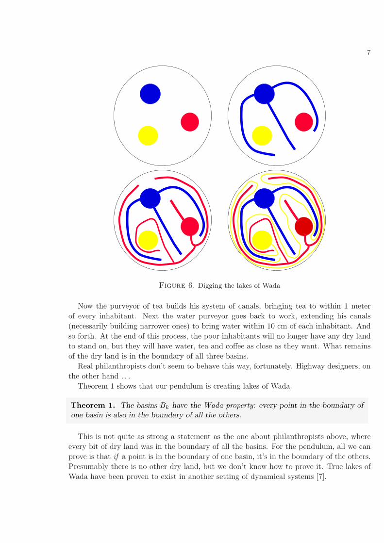
Let me sketch the construction as outlined in [13], illustrating the dangers of philan-thropy; this is illustrated by Figure 6.

Suppose D is an island cursed with three philanthropists, one of whom wants to bringwater to every inhabitant, one tea and one coffee. At the beginning each has a pond of hisown beverage.

First, the purveyor of water digs a system of canals emanating from his pond, and bring-ing water within 100 meters of every inhabitant, never actually touching the surroundingsea or the other ponds, and forming no loops.

Next, the purveyor of coffee builds a system of canals emanating from his pond, bringingcoffee to within 10 meters of every inhabitant, again forming no loops. Since the watercanals make no loops, they don’t cut off any inhabitants from the coffee pond, so this ispossible.

7

Figure 6. Digging the lakes of Wada

Now the purveyor of tea builds his system of canals, bringing tea to within 1 meterof every inhabitant. Next the water purveyor goes back to work, extending his canals(necessarily building narrower ones) to bring water within 10 cm of each inhabitant. Andso forth. At the end of this process, the poor inhabitants will no longer have any dry landto stand on, but they will have water, tea and coffee as close as they want. What remainsof the dry land is in the boundary of all three basins.

Real philanthropists don’t seem to behave this way, fortunately. Highway designers, onthe other hand . . .

Theorem 1 shows that our pendulum is creating lakes of Wada.

inTheorem 1. The basins Bk have the Wada property: every point in the boundary ofone basin is also in the boundary of all the others.

This is not quite as strong a statement as the one about philanthropists above, whereevery bit of dry land was in the boundary of all the basins. For the pendulum, all we canprove is that if a point is in the boundary of one basin, it’s in the boundary of the others.Presumably there is no other dry land, but we don’t know how to prove it. True lakes ofWada have been proven to exist in another setting of dynamical systems [7].

8

The first step in understanding why Theorem 1 is true is to get a grasp on the boundariesof the basins. Most of the material in the next section was developed by Kennedy, Nusseand Yorke [9, 11]. They saw that the basin of a sink often has saddle points on its boundary,and that the stable separatrices of these saddle points make up the accessible boundary ofthe basin. We will first define these words.

Iteration, sinks, saddles, separatrices

Rather than thinking of the differential equation in R3, I find it much easier to think ofthe period mapping (or Poincare mapping) in the plane

P : R2 → R2 given by P :[x(0)x′(0)

]7→[x(2π)x′(2π)

].

This enables me to ignore what motions do between the samples.There is no real loss if we are interested in long-term behavior: iterating m times the

mapping P is equivalent to solving the differential equation for time 2mπ, sampling thesolutions every 2π. But the dynamical objects will now be subsets of the plane rather thanof space: most people visualize objects in the plane much better than in space. In ourcase, the planar objects will be quite complicated enough.

Seen this way, each point sk = (Sk(0), S′k(0)) is an attracting fixed point of P , alsocalled a sink : P (sk) = sk and if a point p is close to sk (within r of it, for instance), itsorbit under P will approach sk. The basin Bk is exactly the set of points p such that thesequence p, P (p), P 2(p), . . . approaches sk.

Sinks can also be periodic of period m > 1. Such sinks are points p such that Pm(p) = p,and such that if a point p1 is sufficiently close to p, the sequence, p1, P

m(p1), P 2m(p1), . . .tends to p. In other words, the solution of the differential equation with (x(0), x′(0)) = p

is an attracting periodic solution of period 2mπ. Our mapping P appears not to have anysuch points (for these values of the parameters), although proving that it has none maywell be an unsolvable problem. But there are infinitely many periodic saddles, as is provedby Theorem 3. And there are infinitely many more whose existence is not guaranteed bythat theorem.

Like a sink, a saddle point for P corresponds to a periodic solution of the original differ-ential equation, but while sinks are associated to stable equilibria, saddles are associatedto unstable equilibria. A periodic solution (x(t), x′(t)) of the differential equation gives asaddle (x(0), x′(0)) of the period mapping P if there is a surface made up of solutions ofthe differential equation that tend to the attracting periodic solution as time tends to +∞,and another surface of solutions that tend to the attracting periodic solution as t→ −∞,i.e., as one travels backwards in time.

An example of a saddle point is the upwards (unstable) equilibrium for an unforceddamped pendulum. Almost all solutions are captured by a stable equilibrium. But excep-tional solutions exist that take an infinite amount of time to approach the vertical, andother solutions take an infinite amount to fall away from the vertical: these solutions makeup two surfaces that intersect along the constant solution corresponding to the unstable

9

equilibrium. The surface of solutions that tend to the vertical in forward time is the stableseparatrix, while the surface of solutions tending to the vertical in backwards time is theunstable separatrix. The intersection of these surfaces with a Poincare plane (i.e. the planet = 0) forms two curves, also referred to as separatrices. Think of the separatrices aswatersheds: for our unforced pendulum, they separate the initial conditions that will goover the top one more time from those that won’t make it.

Mappings R2 → R2 (which might be the period mapping of a time-periodic differentialequation in R2, as in our case) will usually also have sources: fixed or periodic points thatrepel all nearby orbits. The period mapping P for our pendulum has no sources because Pcontracts areas by e(2π)/10 ≈ 0.58, due to the damping ([8], Vol. 2, chapter 8). No mappingcan simultaneously contract areas and map some region to a strictly larger region, as wouldhave to happen near a source. Of course, P−1 has sources wherever P has sinks.

Saddles in the boundary of BkThe computer finds four saddles pk,1, . . . , pk,4 in the boundary of each basin. These saddlesform two cycles of period 2 (i.e., the solutions of the differential equation with initial valuesat these saddles have period 4π). The boundary of the basin appears to be made of theirstable separatrices, as drawn in Figure 7. We will call these separatrices σ+(pk,i): theseare the watersheds that separate the solutions falling into the basin from those that don’t.

-10

-4

6

4

x

y

Figure 7. The stable separatrices of the saddles of period 2 in the boundary of a basin provide

an outline drawing of the basin. Thus this picture is more or less the same as Figure 5, but the

stable manifolds would need to be continued for a very long time to get as much resolution as

figure 5 provides.

In fact, the statement above is not true: the boundaries of the basins are not just theseparatrices; they are much more complicated than that. Consider Wada’s construction:

10

some points of the boundary of the water are on the edge of some water stream, but mostare not. For one thing, points on the edge of a coffee stream are not on the edge of awater stream, even though they are in the boundary of the water: there are water streamsarbitrarily close, but tea streams even closer, etc. Such points are inaccessible by water:you can reach out to them over other streams, with an arbitrarily small motion, but youcannot reach them in a boat. Most points of the common boundary (the separator) arenot accessible from the water, coffee or tea.

Our basins are built in a similar way to the Wada example. Each includes a central“pond” with four canals leading off from it, which dwindle to become infinitely narrowstreams, intermingled with streams belonging to other basins.

In our case, the inward pointing unstable separatrix at each of the four saddles isattracted to the sink, as shown in Figure 8, and provides a path from the sink to the stableseparatrix of the saddle. Thus the stable separatrix is part of the accessible boundary.

inTheorem 2. The accessible boundary of Bk is exactly the union of the stable separa-trices σ+(pk,i) , i = 1, . . . , 4.

The proof consists of looking at Figure 8.

-6.4

-3

2

3

x

y

s

p1

p4

p2

p3

3

-6.4 2

-3

c0

P-1(c1)

q

P-2(c2)P-3(c3)

P(q)

c1

Figure 8. A basin cell; the points P−i(ci) illustrates the proof of Theorem 2.

The colored neighborhood Ck of the sink sk (called a basin cell by [11]) is bounded byarcs of four stable separatrices σ+(pk,i) and arcs of the four unstable separatrices σ−(pk,i),which except for endpoints are contained in the interior of the basin. Thus any accessibleboundary point q of Bk not in

⋃i σ

+(pk,i) will necessarily be outside Ck, and a path

γ : [0, 1] 7→ Bk, γ([0, 1]) ⊂ Bk

11

joining q to sk will intersect one of these four arcs, in points c0. Similarly, the path Pm(γ)will intersect one of these arcs in a point cm. The points zm = P−m(cm) must be on γ,and must converge to q since for any ε > 0, the set γ([0, 1 − ε]) is a compact subset ofBk. Thus Pm(γ([0, 1− ε])) will be inside Ck (or any neighborhood of sk for m sufficientlylarge).

But the cm lie in four compact arcs of⋃i σ−(pk,i), hence P−m(cm) will be very close to

one of the saddles for m large. So q is one of the saddles pk,i, hence on its stable separatrix.This ends the proof of Theorem 2 (or at least a fairly convincing argument; it is not a

rigorous proof, as we will discuss later); now to justify Theorem 1.First, it is enough to show that each accessible point of ∂B0 (the boundary of B0) can

be approached by every other basin. Indeed, every point of ∂B0 can be approached byaccessible points, so if we can show that each accessible point of ∂B0 is in the boundaryof every other basin, then every point of ∂B0 is in the boundary of every other basin.

Second, it is enough to know that the four outward pointing branches of the unstableseparatrices for the four accessible saddles in ∂B0 enter every basin. Indeed, if the fourunstable separatrices σ−(p0,i), for i = 1, 2, 3, 4, enter Bn, then the inverse images of Bnwill accumulate to p0,i, hence to the entire stable separatrix σ+(p0,i). This shows a littlemore: if all four σ−(p0,i) enter Bn, then no curve can enter B0 without crossing a streamof Bn, i.e., entering Bn.

Third, rather than show that the outward-pointing part of each σ−(p0,i) enters all thebasins Bn, for n any integer, it is enough to show that it enters the two neighboring basinsB1 and B−1. We can prove this by induction. Figure 9 shows that the four separatricesσ−(po,i), i = 1, 2, 3, 4 enter the basins B−1 and B1.

Now suppose they enter Bk for some k > 1. But they cannot enter Bk without enteringBk+1, because the σ−k,i enter Bk+1, so that their inverse images give streams of Bk+1 whichthey must ford to enter Bk.

-11

-4

7

4

x

y

B-1

B1

s0

Figure 9. All four of the unstable separatrices from the points p0,i enter both B1 and B−1.

12

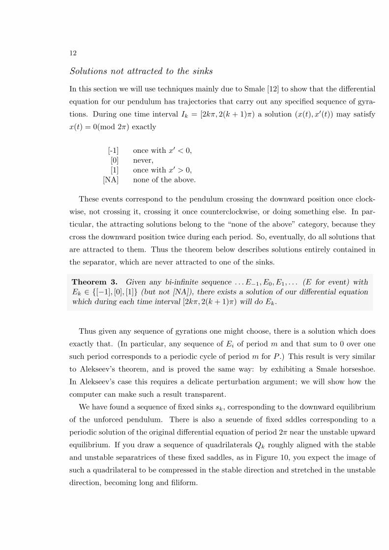
Solutions not attracted to the sinks

In this section we will use techniques mainly due to Smale [12] to show that the differential

equation for our pendulum has trajectories that carry out any specified sequence of gyra-

tions. During one time interval Ik = [2kπ, 2(k + 1)π) a solution (x(t), x′(t)) may satisfy

x(t) = 0(mod 2π) exactly

[-1] once with x′ < 0,[0] never,[1] once with x′ > 0,

[NA] none of the above.

These events correspond to the pendulum crossing the downward position once clock-

wise, not crossing it, crossing it once counterclockwise, or doing something else. In par-

ticular, the attracting solutions belong to the “none of the above” category, because they

cross the downward position twice during each period. So, eventually, do all solutions that

are attracted to them. Thus the theorem below describes solutions entirely contained in

the separator, which are never attracted to one of the sinks.

inTheorem 3. Given any bi-infinite sequence . . . E−1, E0, E1, . . . (E for event) withEk ∈ {[−1], [0], [1]} (but not [NA]), there exists a solution of our differential equationwhich during each time interval [2kπ, 2(k + 1)π) will do Ek.

Thus given any sequence of gyrations one might choose, there is a solution which does

exactly that. (In particular, any sequence of Ei of period m and that sum to 0 over one

such period corresponds to a periodic cycle of period m for P .) This result is very similar

to Alekseev’s theorem, and is proved the same way: by exhibiting a Smale horseshoe.

In Alekseev’s case this requires a delicate perturbation argument; we will show how the

computer can make such a result transparent.

We have found a sequence of fixed sinks sk, corresponding to the downward equilibrium

of the unforced pendulum. There is also a seuende of fixed sddles corresponding to a

periodic solution of the original differential equation of period 2π near the unstable upward

equilibrium. If you draw a sequence of quadrilaterals Qk roughly aligned with the stable

and unstable separatrices of these fixed saddles, as in Figure 10, you expect the image of

such a quadrilateral to be compressed in the stable direction and stretched in the unstable

direction, becoming long and filiform.

13

-15

-4

7

4

x

y

Q0 Q1Q-1

A0

A'0

B0

D0

C0

B'0C'0D'0

Q'0

Figure 10. The quadrilaterals Q−1, Q0, Q1, together with the forward and backwards images

of Q0.

We will describe the set of points

Qk(E0, E1, . . . , EN ) = {p|Pn(p) ∈ Qk+E0+···+En−1 for 0 ≤ n ≤ N}.Label A0, B0, C0, D0 the corners of Q0, as shown in Figure 10. The set P (Q0) is the

curvilinear quadrilateral Q′0, shaded in Figure 10, with vertices A′0, B′0, C

′0, D

′0. The key

property of the image is that it crosses the quadrilaterals Q1 and Q−1, as well as itself, ineach case going from top to bottom (or bottom to top), with the top A0B0 and bottomC0D0 mapping outside these quadrilaterals.

This implies that each of Q0([−1]), Q0([0]), Q0([1]) forms a full-width subrectangle ofQ0. Figure 11 shows the forward and backwards images of Q0, Q−1 and Q1, and a blow-up of showing how these intersect Q0. Indeed the backwards images (light shading) formfull-width subrectangles. Of course, Q1 and Q−1 also contain such subrectangles Q1(E0),etc. The inverse image P−1(QE0(E1)) is then again a (thinner) full-width subrectangleQ0(E0, E1).

Continuing this way, we see that for any finite sequence (E0, E1, . . . , EN ), the corre-sponding set Q0(E0, E1, . . . , EN ) is a full-width subrectangle of Q0. Finally, the assign-ment of an infinite forward trajectory restricts the initial position to an infinite intersectionof nested full-width subrectangles of Q0; such an intersection will be a connected subsetof Q0 connecting one side of Q0 to the other. In fact, it will be a smooth curve, but thisrequires writing some inequalities.

A similar argument shows that any finite backwards trajectory restricts the final po-sition to a full-height subrectangle of Q0, and an infinite backwards trajectory leads toa connected subset joining A0B0 to C0D0 (again in fact a smooth curve). If X,Y ⊂ Q0

are connected subsets, with X joining D0A0 to B0C0 and Y joining A0B0 to C0D0, thenX ∩ Y 6= 0. Thus there is a point realizing any prescribed symbolic trajectory.

14

-15

-4

7

4

x

y

-6

-1.7

-1.4

2.2

x

y

Figure 11. The forward images of Q−1, Q0, Q1, and their intersections with Q0. At right a

blow-up of Q0.

Finally, I claim that the points of Q0([−1]), Q0([0]), Q0([1]) realize possibilities [−1], [0],and [1] above. Figure 12 shows the images of Q0(+1) and Q0(−1) at times

0,2π8,

4π8,

6π8,

8π8,

10π8,

12π8,

14π8,

16π8.

-7

-4

15

4

x

y

Q0 Q1

Q-1

y 4

-4

x7-15

x=-2π

Figure 12. How the quadrilaterals move during one period.

The first set certainly seems to cut the line x = 2π exactly once with y > 0; the secondset seems to cut the line x = 0 once with y < 0.

15

Controlling the pendulum

Imagine that the pendulum is massive, and is being used as a flywheel to control some verydelicate operation, like polishing the mirror of a telescope. An array of lasers is constantlymonitoring the operation, deciding on the fly whether the pendulum should turn clockwise,counterclockwise, or wait until the mirror has been repositioned.

The previous section showed that there are motions of the pendulum performing anyspecified sequence of gyrations, in particular the one required a posteriori by the polisher.But on second thought this seems useless: these motions are extremely unstable, and theslightest error in the initial condition will destroy them, as well as any perturbation of thedifferential equation itself. But if the machine is to perform any work, this will inevitablyperturb the differential equation, in a way which is essentially unpredictable (you cannotpredict how much work one swipe of the polisher will accomplish), and in any case wedon’t know ahead of time the sequence of swipes and stops the task will require.

On third thought, we see that the instability of the specified motions is exactly whatshould make them useful! Suppose that our array of sensors controls the current f(t) thatis forcing the pendulum, changing it from cos(t) to something like

(1 + a(t)) cos(t) (amplitude modulation) or

cos((1 + a(t))t) (frequency modulation),

where a(t) represents the fine-tuning necessary to achieve the desired sequence of gyrations.The point is that we do not have to figure out what sequence we want ahead of time: thesensors can react to the polishing of the telescope on the fly, computing the adjustmenta(t) that is necessary. It is because of the instability that you can keep a(t) small and stillrealize any sequence of gyrations: you don’t need to grind to a halt, compute, and startup again; the corrections can be done smoothly. A useful analogy is skiing: a beginningskier plants his skis well apart, seeking stability, which is fine until he tries to turn anddiscovers he can’t. An expert skier, with skis parallel and touching, is highly unstable,and a slight wiggle of the hips will allow him to negotiate a mogul. Of course he doesn’tplot his entire path at the top of the mountain; he calculates the slight adjustments a(t)as they are needed.

inTheorem 4. For any sequence of events E0, E1, . . . and any sufficiently small dis-turbance b(t) of the forcing term cos t, there exists a function a(t) of the same orderof magnitude as b(t) and an initial condition x(0), x′(0) such that the solution of thedifferential equation

x′′ + .1x′(t) + sin(x) + b(t) =(1 + a(t)

)cos t

with those initial conditions realizes the specified sequence of events.

This result is fairly obvious: choose a(t) as the pendulum approaches the upwardsposition so as to speed it up or slow it down as required. The problem is how to computethe a(t), in terms of available data. Clearly a(t) should only depend on the values of b up

16

to time t− 2π; it should not depend on the specified sequence of events very far ahead, asthis is unknown. How small can a(t) be made? How far ahead in the required sequence ofevents does it need to look? How sensitive is it to small errors in the sensors? . . .

Control and celestial mechanics

To return to celestial mechanics for a moment, it is interesting to note that when sendinga spaceship to visit the outer solar system, NASA uses the instabilities of the differentialequations describing gravity in much the same way as we have used the instabilities of thependulum. It is well beyond present day engineering to send a spaceship out of the solarsystem by simply using its fuel to accelerate it. Instead, it is allowed to “fall” into the sun,with an orbit which passes close to Venus. It then loops around Venus; we can imaginethat it is the “satellite” in the three body system consisting of itself, Venus and the sun.

This system is similar to Alekseev’s (somewhat more complicated: a Poincare sectionwould need to be 4-dimensional rather than 2), and one can prescribe an orbit so that thespace ship steals a tiny amount of potential energy from Venus, speeding up enormously inthe process, and ends up in a very unstable state where a small push by guidance rocketscan put it on the path to Jupiter.

This scenario is then repeated near Jupiter, Saturn and Uranus, with the spaceship eachtime gaining momentum, and using small pushes to head itself in the direction of the nextdestination. Thus the chaos of the solar system is essential to its exploration.

What is proved?

To what extent does this paper prove anything? As written, no statement is provedanywhere: for the punchline we just looked at a computer picture. How do we know thatthese pictures are right? I will not address the possibility that the programs have essentialbugs, and are computing something other than what I think, or the esoteric possibilitythat the computer arithmetic is wrong. But even if the computer is computing exactlywhat I think, that is still only an approximation to solutions of the differential equations;we need to quantify the quality of the approximation. The contribution of round-off erroralso should be addressed.

Actually, many of the results are not hard to prove rigorously, namely all those wherewe have to show that after time 2π, solutions are within some fairly large ε of the valuewhich the computer drawings suggest.

Good estimates of long-term errors of numerical approximations to solutions of differen-tial equations are notoriously hard to come by, but that is not really a problem here. First,we do not need good estimates (solutions only need to be accurate to about 0.1); second,the time considered is not long (2π); and most important, the differential equation hasa small Lipschitz constant (

√2.001 < 1.42). Errors in solutions to differential equations

grow at most exponentially, at a rate ekt, where t is time (in our case, 2π) and k is theLipschitz constant; with k < 1.42, errors grow at a fairly small interest rate, and can becontrolled for a short time.

17

Using these numbers, a straightforward computation using the fundamental inequality([8], Chapters 4 and 6) shows that if the initial velocity satisfies |x′(0)| < 3, then Euler’smethod with step length h = .000002 gives results accurate to 0.1 after time 2π. Moreover,the same inquality shows that roundoff-error contributes a much smaller error yet. Thisis not a good way to do such numerics; better numerical methods [5] give much betterestimates. For instance, formula (14) of [2] can be used to show that the fourth orderRunge-Kutta method with step .005 has more than the needed precision.

A word of caution, though. The elementary bound above says that errors of all typesare multiplied by at most e2π1.42 ≈ 7 500 over one time period. It is not too difficultto improve this to e2π1.1 ≈ 1 000, and one could improve it further. But one could notimprove it very much further.

Consider for example the completely unavoidable error caused by the computer’s in-ability to handle numbers with infinite precision. If it handles numbers to 16 significantdigits, you may think you are starting at a saddle point, but your initial error (the distancebetween the saddle point and where you really are) may be as great as 10−16. The largesteigenvalue λ of the linearization of P at the fixed saddles in the Qk is about 321 (accordingto the computer). As long as you are in the region where P is approximately its lineariza-tion at this saddle, errors of all types are expanded by a factor of λ over one time period,and hence λm over m time periods. So after m iterations the error will have mushroomedto 10−16(321m): for m = 7 the initial minute error will have grown to 35. But alreadyfor an error of 1, you will have been booted out of the region where the linearization is areasonable approximation to reality.

Thus no numerical method can guarantee even one digit of accuracy after six timeperiods, if we are computing with 16 significant digits. In fact, the reality is much worsethan that, and I wouldn’t trust anything after four time periods without some good reason.

A posteriori bounds

Good reasons to trust solutions are available: I advocate extrapolation, as described in [8],Chapter 3. Let us write uh(t) the numerical approximation solution of some differentialequation given by the standard 4th order Runge-Kutta method, and with uh(0) = a. Thenthe theory asserts that for each fixed t the approximation uh(t) converges to the value ofthe solution u(t), and that we have an asymptotic development

uh(t) = u(t) + Ch4 + o(h4).

The exponent 4 is a feature of this approximation procedure; others have different expo-nents.

If for some h we know uh(t), uh/2(t) and uh/4(t), and we assume that we have an asym-totic development of the form uh(t) = u(t) + Chk + o(hk) for some k, we can extrapolatethe values of k and of C from the values of the approximate solutions:

k =1

log 2log∣∣∣∣ uh(t)− uh/2(t)uh/2(t)− uh/4(t)

∣∣∣∣ and C =2k

2k − 1uh(t)− uh/2(t)

hk.

18

Now suppose we calculate uh/2m(t) for a range of values of m, focusing on the expressionfor k above. The theory says that as m increases, the value of k should approach 4, butthat doesn’t take round-off error into account; typically the value of k will approach 4as m increases, then veer away from 4 as round-off error takes over. If there is a rangeof values of m where k is close to 4, the approximation is happening the way the theorypredicts, and we can probably trust the corresponding estimate of the error. The followingdata illustrates this for our differential equation, solved for 0 ≤ t ≤ 16π, i.e., for 8 periods.We will start with the two initial positions (7.15859, .14097) and (7.16859, .14097). Theextrapolations we find are

first solution second solutionsteps order error order error

612 22.45 86.2224 3.07 2.67 1.05 41.4848 −1.79 9.31 2.61 6.7796 3.26 0.96 −0.15 6.84

192 −0.44 1.31 −1.09 14.64384 −2.01 5.27 3.02 1.80768 −0.06 5.48 4.96 .057

1536 5.13 .16 4.19 0.003What we can read off from this is that the first approximation never becomes reliable;

the order is never close to 4. In particular, there is no reason to think that the quantityin the “error” column is actually an estimate of the error. But the second appears to beconverging nicely, with the order approaching 4, and probably the error estimate of .003 isreliable. Thus although any estimate we make a priori for a bound for the error is boundto be wildly pessimistic, after the computation we can make a good guess as to how reliableit is.

Questions and observations

(1) Are there any periodic sinks other than the attracting fixed points we found? Ihave no idea how to attack this problem. For one thing, I don’t trust computerdrawings on this point: in many instances I eventually found sinks whose basinswere too small to be visible on computer drawings unless you knew where to look.

For another, the answer might depend in the most delicate way on the param-eters: there definitely are other attracting fixed points when the forcing term is1.22 cos t instead of cos t; for example, there is a sink of period 3, where solu-tions go from the point with coordinates x = −1.29785, y = 1.0025 to the pointx = −1.3349, y = −.21286, to the point x = −3.004469, y = .17586, and then backto the first point . . . . In fact, with those parameters there are at least two moresinks of period 3, in addition to all the translates of the three sinks by 2π.

In fact, this problem may be unsolvable. Milnor’s candidate for the simplestunsolvable problem of mathematics is the question: “does the polynomial x2 − 1.5

19

have an attracting cycle?” Of course, if it does have one, one can find it with afinite amount of work. But if it doesn’t have one, there may be no proof of thisfact.

(2) Is the complement of all the basins Bk of measure 0? This would mean that withprobability 1 every initial point is attracted to a sink. I think this is the case,but have no solid grounds for this belief. Even the computer isn’t very definite(and besides, this is one point where numerical error might really be important:the perturbations of the period mapping due to errors of integration and round-offmight affect the probability of being attracted to a sink.)

Acknowlegements

I wish to thank Stan Wagon, Mukund Thattai and an anonymous referee for many helpfulcomments and suggestions.

Bibliography

[1] V.M. Alekseev, On the capture orbits for the three-body problem for negative energyconstant, Uspekhi Mat. Nauk 24, 185–186 (1969)

[2] L. Bieberbach, On the remainder of the Runge-Kutta formula in the theory of ordi-nary differential equations, Z.A.M.P.,II (1951), 233–248

[3] R. Borelli and C. Coleman, Computers, lies and the fishing season, College Math.Jour., 25,5 (1994) 401–412.

[4] L.E.J Brouwer, Zur Analysis Situs, Math. Annalen, Vol. 68 (1910), 422–434[5] P. Henrici, Discrete variable methods in ordinary differential equations, Wiley, 1962.[6] B. Hinkle, J. Hubbard, and B. West, Planar Systems and Planar Iterations, to be

published by Springer Verlag. These programs constitute the latest version of MacMathby Hubbard and West, originally published by Springer Verlag in 1991.

[7] J. Hubbard and R. Oberste-Vorth, Henon mapping in the complex domain II: Pro-jective and inductive limits of polynomials, Proceedings of the NATO summer conferencein Hillerod, 1993.

[8] J. Hubbard and B. West, Differential Equations, a dynamical systems approach, Vol.I, Springer Verlag (1992) and Vol. II, Springer Verlag (1994)

[9] J. Kennedy and J. Yorke, Basins of Wada, Physica D 51 (1991), 213–255.[10] J. Moser, Stable and random motions in dynamical systems, Annals of Mathematics

Studies, Princeton University Press, 1973[11] H. Nusse and J. Yorke, Wada basin boundaries, preprint March 1994, 1–51.[12] D. Smale, Diffeomorphisms with many periodic points, Differential and combinato-

rial topology, edited by S. S. Cairns, Princeton U. Press (1965) 63–80.[13] K. Yoneyama, Theory of continuous set of points, Tohoku Math. J., 11–12 (1917),

43.