the ford-fulkerson method

1

Course Outline

Introduction to Iterative Improvement Strategy The maximum-flow problem ALGORITHM ShortestAugmentingPath(G) Assignment 1 Maximum Matching in Bipartite Graphs ALGORITHM MaximumBipartiteMatching(G) Assignment 2 The Stable Marriage Problem Stable marriage algorithm Assignment 3

Iterative Improvement

The greedy strategy constructs a solution to an optimization problem piece by piece, always adding a locally optimal piece to a partially constructed solution.

Iterative improvement starts with some feasible solution and proceeds to improve it by repeated applications of some simple step.

This step typically involves a small, localized change yielding a feasible solution with an improved value of the objective function.

When no such change improves the value of the objective function, the algorithm returns the last feasible solution as optimal and stops.

2

Some Obstacles in Iterative Improvement

First, we need an initial feasible solution. Second, it is not always clear what changes

should be allowed in a feasible solution so that we can check efficiently whether the current solution is locally optimal and, if not, replace it with a better one.

Third—and this is the most fundamental difficulty— is an issue of local versus global extremum (maximum or minimum).

Fortunately, there are important problems that can be solved by iterative improvement algorithms. The most important of them is linear programming.3

The Maximum-Flow Problem

The problem of maximizing the flow of a material through a transportation network (pipeline system, communication system, electrical distribution system, and so on).

A transportation network can be represented by a connected weighted digraph with n vertices numbered from 1 to n and a set of edges E, with the following properties: It contains exactly one vertex with no entering edges, called

the source and assumed to be numbered 1. It contains exactly one vertex with no leaving edges; called

the sink and assumed to be numbered n. The weight uij of each directed edge (i, j) is a positive integer,

called the edge capacity.

It is assumed that the total amount of the material entering an intermediate vertex must be equal to the total amount of the material leaving the vertex (flow-conservation requirement)

4

The Maximum-Flow Problem

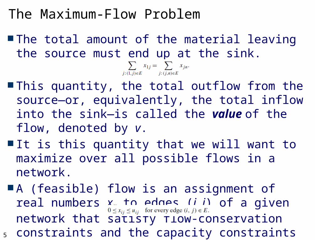
The total amount of the material leaving the source must end up at the sink.

This quantity, the total outflow from the source—or, equivalently, the total inflow into the sink—is called the value of the flow, denoted by v.

It is this quantity that we will want to maximize over all possible flows in a network.

A (feasible) flow is an assignment of real numbers xij to edges (i, j) of a given network that satisfy flow-conservation constraints and the capacity constraints

5

Iterative Improvement Strategy for Max-Flow Problem Start with the zero flow Then, on each iteration, try to find a path from

source to sink along which some additional flow can be sent. This path is called flow augmenting.

If a flow-augmenting path is found, adjust the flow along the edges of this path to get a flow of an increased value and try to find an augmenting path for the new flow.

If no flow-augmenting path can be found, conclude that the current flow is optimal, stop.

The strategy is called the augmenting-path method, or the Ford-Fulkerson method.

6

the Ford-Fulkerson method

Start with the zero flow Then, on each iteration, try to

find a path from source to sink along which some additional flow can be sent. This path is called flow augmenting.

If a flow-augmenting path is found, adjust the flow along the edges of this path to get a flow of an increased value and try to find an augmenting path for the new flow.

If no flow-augmenting path can be found, conclude that the current flow is optimal, stop.

7

How to find an augmenting path

consider paths from source to sink in the underlying undirected graph in which any two consecutive vertices i, j are either connected by a directed edge from i to j with some

positive unused capacity rij = uij – xij (so that we can increase the flow through that edge by up to rij units), or

connected by a directed edge from j to i with some positive flow xji (so that we can decrease the flow through that edge by up to xji units).

The first kind of edges are called forward edges, the second ones are backward edges.

Example: for the path 1→4→3←2→5→6, what are the forward edges? The backward edge?

8

the Ford-Fulkerson / augmenting-path method For a given flow-augmenting path, let r be the minimum

of all the unused capacities rij of its forward edges and all the flows xji of its backward edges.

It is easy to see that if we increase the current flow by r on each forward edge and decrease it by this amount on each backward edge, we will obtain a feasible flow whose value is r units greater than the value of its predecessor.

The augmenting-path method does not indicate a specific way for generating flow-augmenting paths.

Fortunately, there are several ways to generate flow-augmenting paths efficiently.

The simplest of them uses breadth-first search to generate augmenting paths with the least number of edges, called shortest-augmenting-path or first-labeled-first-scanned algorithm by J. Edmonds and R. M. Karp.

9

The Shortest-Augmenting-Path Algorithm The labeling refers to marking a new (unlabeled) vertex with two labels.

The first label indicates the amount of additional flow that can be brought from the source to the vertex being labeled.

The second label is the name of the vertex from which the vertex being labeled was reached.

Add the + or − sign to the second label to indicate whether the vertex was reached via a forward or backward edge, respectively.

The source can be labeled with ∞, −. For the other vertices, the labels are computed as follows.

If unlabeled vertex j is connected to the front vertex i of the traversal queue by a directed edge from i to j with positive unused capacity rij = uij − xij , then vertex j is labeled with lj, i+, where lj = min{li, rij}.

If unlabeled vertex j is connected to the front vertex i of the traversal queue by a directed edge from j to i with positive flow xji , then vertex j is labeled with lj, i -, where lj =min{li,xji}.

If this labeling ends up labeling the sink, the current flow can be augmented by the amount indicated by the sink’s first label.

If the sink remains unlabeled after the traversal queue becomes empty, the algorithm returns the current flow as maximum and stops.

10

Exercises

Apply the shortest-augmenting path algorithm to find a maximum flow in the following networks:a.

b.

12

Assignment 1 (a group of two students)

As an alternative to the shortest-augmenting-path algorithm, Edmonds and Karp suggested the maximum-capacity-augmenting-path algorithm, in which a flow is augmented along the path that increases the flow by the largest amount.

Implement both these algorithms in the language of your choice and perform an empirical investigation of their relative efficiency.

Due date: 19/12/2013

13

Network Cuts

A cut is formed by partitioning vertices of a network into some subset X containing the source and X, the complement of X, containing the sink.

A cut is the set of all the edges with a tail in X and a head in X .

If all the edges of a cut were deleted from the network, there would be no directed path from source to sink.

14

Network Cuts

The capacity of a cut C(X, X), denoted c(X, X), is defined as the sum of capacities of the edges that compose the cut.

What are the capacities of the following cuts? A minimum cut is a cut with the smallest

capacity. What is it in the following network? Max-Flow Min-Cut Theorem: The value of a

maximum flow in a network is equal to the capacity of its minimum cut.

15

Complexity of the shortest-augmenting-path algorithm Edmonds and Karp proved in their paper that the number of

augmenting paths needed by the shortest-augmenting-path algorithm never exceeds nm/2, where n and m are the number of vertices and edges, respectively.

Since the time required to find a shortest augmenting path by breadth-first search is in O(n + m) = O(m) for networks represented by their adjacency lists, the time efficiency of the shortest-augmenting-path algorithm is in O(nm2).

More efficient algorithms for the maximum-flow problem are known. Some of them implement the augmenting-path idea in a more efficient manner. Others are based on the concept of a preflow, i.e a flow that satisfies the capacity constraints but not the flow-conservation requirement.

Any vertex is allowed to have more flow entering the vertex than leaving it. A preflow-push-algorithm moves the excess flow toward the sink until the flow-conservation requirement is reestablished for all intermediate vertices of the network. Faster algorithms of this kind have worst-case efficiency close to O(nm).

16

17

Course Outline


Maximum Matching in Bipartite Graphs

problem of pairing elements of two sets represent elements of two given sets by vertices

of a graph, with edges between vertices that can be paired

A matching in a graph is a subset of its edges with the property that no two edges share a vertex

A maximum matching/ a maximum cardinality matching is a matching with the largest number of edges

18

What is the maximum matching for the graph above? Is it unique?

Maximum Matching in Bipartite Graphs

The maximum-matching problem is the problem of finding a maximum matching in a given graph.

For an arbitrary graph, this is a rather difficult problem. We limit our discussion in this course to the simpler case of bipartite graphs: all the vertices can be partitioned into two disjoint

sets V and U, not necessarily of the same size, so that every edge connects a vertex in one of these sets to a vertex in the other set.

A graph is bipartite if its vertices can be colored in two colors so that every edge has its vertices colored in different colors; such graphs are also said to be 2-colorable.

A graph is bipartite if and only if it does not have a cycle of an odd length.

19

The iterative-improvement technique to the maximum-cardinality-matching problem Example of a bipartite graph

We will assume that the vertex set of a given bipartite graph has been already partitioned into sets V and U as required by the definition

Let M be a matching in a bipartite graph G = <V, U, E>. How can we find a new matching with more edges?

if every vertex in either V or U is matched (has a mate), i.e., serves as an endpoint of an edge in M, this cannot be done and M is a maximum matching.

Therefore, to improve the current matching, both V and U must contain unmatched (also called free) vertices, i.e., vertices that are not incident to any edge in M.

For example, for the matching Ma = {(4, 8), (5, 9)} in the graph above, vertices 1, 2, 3, 6, 7, and 10 are free, and vertices 4, 5, 8, and 9 are matched.

we can increase a current matching by adding an edge between two free vertices.

For example, adding (1, 6) to the matching Ma yields a larger matching Mb = {(1, 6), (4, 8), (5, 9)}.

now try to find a matching larger than Mb by matching vertex 2.

The only way to do this would be to include the edge (2, 6) in a new matching.

This inclusion requires removal of (1, 6), which can be compensated by inclusion of (1, 7) in the new matching.

This new matching Mc = {(1, 7), (2, 6), (4, 8), (5, 9)} is shown below:

In general, we increase the size of a current matching M by constructing a simple path from a free vertex in V to a free vertex in U whose edges are alternately in E−M and in M.

Such a path is called augmenting with respect to the matching M.

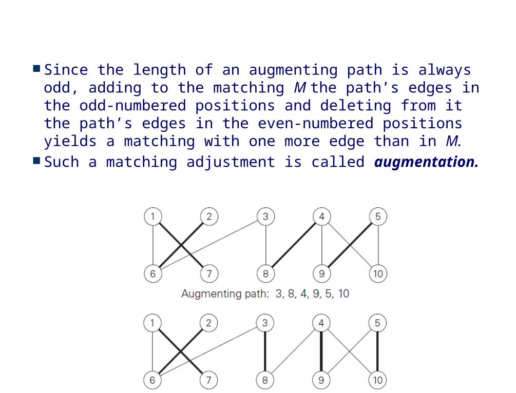
Since the length of an augmenting path is always odd, adding to the matching M the path’s edges in the odd-numbered positions and deleting from it the path’s edges in the even-numbered positions yields a matching with one more edge than in M.

Such a matching adjustment is called augmentation.

A matching M is a maximum matching if and only if there exists no augmenting path with respect to M.

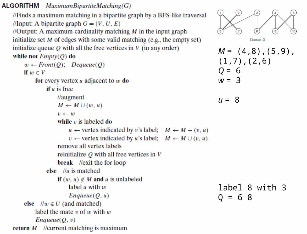
For constructing a maximum matching in a bipartite graph: Start with some initial matching (e.g., the empty set). Find an augmenting path and augment the current matching

along this path. Use BFS-like traversal of the graph that starts simultaneously at all

the free vertices in one of the sets V and U, say, V. rules for labeling vertices during the BFS-like traversal of the graph

Case 1: (the queue’s front vertex w is in V) If u is a free vertex adjacent to w, it is used as the other

endpoint of an augmenting path; so the labeling stops and augmentation of the matching commences. The augmenting path is obtained by moving backward along the vertex labels to alternately add and delete its edges to and from the current matching.

If u is not free and connected to w by an edge not in M, label u with w unless it has been already labeled.

Case 2: (the front vertex w is in U) In this case, w must be matched and we label its mate in V

with w. When no augmenting path can be found, terminate the

algorithm and return the last matching, which is maximum.

w = 1

u = 6

M = (4,8), (5,9), (1,6)v = 1

Q = 2 3

w = 2

u = 6

label 6 with 2Q = 3 6

w = 3

u = 8


w = 6


w = 8


w = 1

u = 7

M = (4,8),(5,9),(1,6),(1,7)v = 1

u = 6; M =(4,8),(5,9),(1,7)v = 2;M = (4,8),(5,9),(1,7),(2,6)Q = 3

M = (4,8),(5,9),(1,7),(2,6)Q = 3w = 3u = 6

label 6 with 3Q = 6

M = (4,8),(5,9),(1,7),(2,6)Q = 6w = 3

u = 8


Q = 6 8w = 6


Q = 8 2w = 8


M = (4,8),(5,9),(1,7),(2,6)Q = 2 4w = 2u = 6

M = (4,8),(5,9),(1,7),(2,6)Q = 4w = 4u = 8

M = (4,8),(5,9),(1,7),(2,6)Q = 4w = 4u = 9

label 9 with 4Q = 9

M = (4,8),(5,9),(1,7),(2,6)

w = 4u = 10M =(4,8),(5,9),(1,7),(2,6),(4,10)v = 4u = 8M = (5,9),(1,7),(2,6),(4,10)v = 3M = (5,9),(1,7),(2,6),(4,10),(3,8)Q = []

Exercise 10.3

How efficient is the maximum-matching algorithm? Each iteration except the last one matches two

previously free vertices—one from each of the sets V and U.

Therefore, the total number of iterations cannot exceed n/2 + 1, where n = |V | + |U| is the number of vertices in the graph.

The time spent on each iteration is in O(n + m), where m = |E| is the number of edges in the graph.

Hence, the time efficiency of the algorithm is in O(n(n + m)).

42

Assignment 2

Implement the maximum-matching algorithm of this section in the language of your choice. Experiment with its performance on bipartite graphs with n vertices in each of the vertex sets and randomly generated edges (in both dense and sparse modes) to compare the observed running time with the algorithm’s theoretical efficiency.

43

44

Course Outline


The Stable Marriage Problem

Consider a set Y = {m1, m2, . . . , mn} of n men and a set X = {w1, w2, . . . , wn } of n women.

Each man has a preference list ordering the women as potential marriage partners with no ties allowed.

Similarly, each woman has a preference list of the men, also with no ties.

45


A marriage matching M is a set of n (m, w) pairs whose members are selected from disjoint n-element sets Y and X in a one-one fashion, i.e., each man m fromY is paired with exactly one woman w from X and vice versa.

A pair (m, w), where m ∈ Y, w ∈ X, is said to be a blocking pair for a marriage matching M if man m and woman w are not matched in M but they prefer each other to their mates in M. For example, (Bob, Lea) is a blocking pair for the marriage matching M = {(Bob, Ann), (Jim, Lea), (Tom, Sue)}

46


A marriage matchingM is called stable if there is no blocking pair for it; otherwise, M is called unstable. According to this definition, the marriage matching in Figure 10.11c is unstable.

The stable marriage problem is to find a stable marriage matching for men’s and women’s given preferences.

47

Stable marriage algorithm

Trace it on the following input:

48

Analysis

The stable marriage algorithm terminates after no more than n2 iterations with a stable marriage output.

Proof by contradiction that the algorithm produces stable matching: Suppose that M is unstable. Then there exists a blocking pair of a man m and a woman w

who are unmatched in M and such that both m and w prefer each other to the persons they are matched with in M.

Since m proposes to every woman on his ranking list in decreasing order of preference and w precedes m’s match in M, m must have proposed to w on some iteration.

Whether w refused m’s proposal or accepted it but replaced him on a subsequent iteration with a higher-ranked match, w’s mate in M must be higher on w’s preference list than m because the rankings of the men matched to a given woman may only improve on each iteration of the algorithm.

This contradicts the assumption that w prefers m to her final match in M.

49

Analysis

The stable marriage algorithm has a notable shortcoming. It is not “gender neutral.”

By tracing the algorithm on the following instance of the problem:

The algorithm obviously yields the stable matching M = {(man 1, woman 1), (man 2, woman 2)}.

In this matching, both men are matched to their first choices, which is not the case for the women.

The algorithm always yields a stable matching that is man-optimal: it assigns to each man the highest-ranked woman possible under any stable marriage.

Of course, this gender bias can be reversed, but not eliminated, by reversing the roles played by men and women in the algorithm, i.e., by making women propose and men accept or reject their proposals.

50

Exercise 10.4

51

Assignment 3

Implement the stable-marriage algorithm given in this lecture so that its running time is in O(n2). Run an experiment to ascertain its average-case efficiency.

Due date for both implementations (max matching and stable marriage): 9 January 2014

Selamat berlibur (dan mengerjakan tugas)

52

the ford-fulkerson method

Documents

feasible flow

flow augmenting

flowaugmenting path

new flow

additional flow

maximumflow problemthe

flowconservation constraints

maxflow problemstart