the fourteenth dubrovnik economic conference

Annabelle Mourougane and Lukas Vogel The Impact of Selected Structural Reforms: Speed of Adjustment and Distributional Effects Hotel "Grand Villa Argentina", Dubrovnik

Draft version

June 25 - June 28, 2008 Please do not quote

The Fourteenth Dubrovnik Economic Conference

Organized by the Croatian National Bank

DRAFT

1

THE IMPACT OF SELECTED STRUCTURAL REFORMS: SPEED OF ADJUSTMENT AND

DISTRIBUTIONAL EFFECTS

By Annabelle Mourougane and Lukas Vogel1

1. Introduction and main findings

1. The long-term impact of labour market reforms on economic performance has been studied in

depth, in particular in the context of the revisited 2006 OECD Jobs Strategy. The impact of institutions on

adjustment to temporary shocks is also well-documented (Duval et al., 2007; Ernst et al., 2007; Inklaar and

Timmer, 2006). By contrast, only very few analyses have focused on transitional effects of structural

reforms and adjustments from one steady state to another. It is indeed not easy to disentangle effects

coming from a shift in the steady state from transitional dynamic effects. The lack of analysis also reflects

the limited temporal dimension of institutional variables.

2. Still, analysing the adjustment path is important for political economy reasons. It gives an idea of

the time needed to see the impact of reforms on economic performance and the amplitude of the short-term

transition costs, thereby putting long-term benefits in perspective. Having a clearer idea of the adjustment

lags associated with structural policies is also useful for macroeconomic stabilisation decisions and helps

policymakers gauge the complementarities between structural adjustment and monetary or fiscal

accommodation.

3. Against this background, this paper examines the nature and the length of economic adjustment

to selected structural reforms, drawing on a variety of approaches. First, the impact of institutional reforms

on equilibrium unemployment is analysed through simple descriptive analyses. Second, simulations using

two different types of models, namely small macro-economic neo-Keynesian models and a micro-founded

dynamic general equilibrium (DGE) model, give insight on how existing rigidities in labour and product

markets and characteristics of financial markets affect the pace of adjustment to structural reforms. They

also help to quantify the impact of monetary policy reaction on the speed of adjustment and illustrate the

distributional effects of labour market reforms.

4. The main conclusions are the following:

The descriptive analysis suggests that the impact of labour market reforms, including a change in

the tax wedge, the replacement ratio or anti-competitive product market regulation2 on structural

unemployment is very gradual and peak only after 5 to 10 years.

Employment adjustment costs appear to have only a limited effect on the pace of adjustment to

labour market reforms and the influence of price adjustment costs on output dynamics is found to

be marginal. This result is robust to the choice of the policy variables (income tax, benefit

1 . The authors are currently working at the OECD Economics Department. They are grateful to Jonathan

Coppel, Jørgen Elmeskov, Claude Giorno, Peter Hoeller, Vincent Koen and Jean-Luc Schneider for helpful comments

and suggestions. The views expressed in this paper do not necessarily reflect those of the OECD.

2. Evidence of complementarities between product and labour market reforms can be found in Nicoletti and

Scarpetta (2005).

DRAFT

2

replacement rate or employer social security contributions) and holds for both neo-Keynesian and

DGE-based simulations.

Full access to well-performing financial markets will also affect adjustment speed by easing firms

and household liquidity constraints. DGE-based simulations suggest however that the presence of

liquidity-constrained households would be partly offset by a stronger monetary policy reaction.

The final effect on the adjustment of real variables would be limited. By omitting capital

adjustments, these simulations may nonetheless underestimate the effects of easing household

liquidity constraints on adjustment to structural reforms.

Macro-economic policy can have a sizable impact on the magnitude of short-term transition costs.

In particular, monetary policy reaction can speed up the adjustment to a new equilibrium though to

a varying degree in the different OECD countries or regions. Reforms in individual euro area

countries are likely to trigger only little or no policy reaction, unless there is an area-wide effort to

implement structural reforms. The speed of adjustment is found to be faster in the United States

than in the euro area, reflecting mostly a higher sensitivity of domestic demand to real interest

rates. This result appears to be robust to the choice of the euro area monetary policy reaction.

The size of international economic spillovers of structural reforms is found to be very small.

Although the examined labour market reforms are estimated to boost aggregate consumption and

output immediately after implementation, they are the source of substantial distributional effects.

Liquidity-constrained households may incur transitional losses after a cut in the benefit

replacement ratio. But a suitable compensation scheme could reduce these potential short-term

losses. A reduction in income tax rates or employer social security contributions would not involve

transitory losses for liquidity-constrained households.

2. Modelling the short-term impact of structural reforms

5. There is little analysis on the short-term impact of structural reforms on economic performance,

the main reason being the limited temporal variation of institutional variables. Studies based on single-

equation cross-country panel estimations or industry-level difference-in-differences approaches have been

widely used in the literature (Belot and van Ours, 2001; Bassanini and Duval, 2006; OECD, 2007). In these

approaches, transmission channels from structural policies to macroeconomic performance are considered

in isolation and a relationship links a performance indicator (e.g. the unemployment rate or productivity) to

institutional variables. These analyses can be useful to assess the long-term impact of structural reforms

but provide little information on the dynamics of adjustment as they are most of the time based on static

equations. Empirical studies using institutional variables in panel estimation usually display limited time

variation, so that only a small set of variables can be tested at a time. Moreover, these approaches fail to

properly capture the fact that institutions that work in one way in one country may work differently

elsewhere because the rest of the institutional structure differs (Duval and Vogel, 2008; Freeman, 1998).

Interactions between institutions are usually proxied by product terms of the respective regressors but the

ability of this approach to analyse a sequence of reforms tends to be rather limited (Dreger et al., 2007).

6. Most of the papers that have attempted to examine the short-term effects of structural reforms on

economic performance rely on dynamic models, either neo-Keynesian or micro-founded DGE models (e.g.

Bean, 1998; Coenen et al., 2007; Everaert and Schule, 2006).3 Neo-Keynesian models incorporate most of

3. There is, on the other hand, a richer literature on the effects of institutions on macroeconomic resilience

and the absorption of exogenous shocks. Examples include Campolmi and Faia (2007), Duval et al. (2007), Ernst et

al. (2007), Grenouilleau et al. (2007) and Smets and Wouters (2005).

DRAFT

3

the traditional properties of large macroeconomic models (Box 1). They are well-suited to analyse the

short-term impact of structural reforms as the lag structure of the model is determined by the empirical fit,

i.e. country specificities. A major drawback is however, that it is not possible to introduce many relevant

institutional variables directly in the model, the main exceptions being tax- and expenditure-related data.

Simulations are thus generally limited to illustrative shocks on NAIRUs or mark-ups, the objective being

to describe the adjustment mechanisms at play (Bean, 1998; Duval and Elmeskov, 2005; Hunt and Laxton,

2004). The ex post impact of reforms can also be examined using a two-step procedure whereby the shock

on the NAIRU or mark-up is first calibrated off model using external information, for instance the impact

of institutions on a reduced-form unemployment equation, and then simulated with a macroeconomic

model. However, this strategy leads to unbiased estimates only if direct effects of institutions on economic

performance are negligible.

Box 1. Main features of the neo-Keynesian small models

This box provides an overview of small models used to simulate a NAIRU shock in the United States, the euro area and France. A detailed description of the main equations is provided in Annex 2. Most behavioural equations are estimated in an error-correction form. The models are backward-looking: agents’ expectations are treated implicitly by the inclusion of lags in the dependent variables. Real short-term rates are determined endogenously through a Taylor rule, with equal weights on inflation and the output gap.

The short-term behaviour of the model is influenced by standard Keynesian features through imperfectly flexible wages and prices, liquidity-constrained consumption, capital adjustment cost and labour hoarding. In the short term output is thus determined by demand. Unemployment and the output gap are important determinants of wage and price adjustments.

In the medium to long-run, the supply side of the economy, which is modelled through a neo-classical production function, plays a prominent role. Factor demands are derived from profit maximisation. Prices and wages adjust and modify price competitiveness as well as firms’ profit and capital stock. Output and unemployment move back to their long-term equilibrium levels.

More precisely, a decline in the NAIRU will have the following effects:

Potential output immediately jumps, leading to a negative output gap and a positive unemployment gap.

Gaps put downward pressure on prices and wages.

Employment rises following the decline in real wages and as labour supply increases very slowly the unemployment rate declines. Consumption and investment also react to these price and wage effects.

Gaps and their resulting disinflationary effects trigger cuts in the real interest rate, which stimulate demand.

In the long run, the unemployment rate and output reach their equilibrium level, closing gaps. Inflation is coming back to baseline.

The main difference in an open economy is that price and demand dynamics also affect trade flows. Consequently, the implementation of a structural reform in one specific country generates externalities for its major trading partners.

7. Alternatively the impact of structural reforms can be evaluated using DGE models that are

explicitly derived from the optimisation of agents’ behaviour under constraints (Box 2). This approach

allows a wide range of structural reforms to be examined and possible spillovers between the variables to

DRAFT

4

be taken into account.4 The use of DGE models presents a number of advantages. First, these models are

less subject to the Lucas critique as they are based on structural equations with sound microeconomic

foundations. Second, it is possible to assess alternative policies through their effects on consumer welfare.

Third, the DGE approach allows studying the distributional effects of reforms. Finally, DGE models

encompass dynamic effects and are well-honed to examine the adjustment to changes in economic

structure and policy. However, the lag structure reflects the optimisation-based micro-foundations and is

generally limited and similar across regions or countries. Consequently, DGE results may tend to

overemphasise similarities and to attribute differences to shocks rather than to economic structures. The

empirical validation of DGE models is an important concern, but also an active field of economic research.

Both the model dynamics and steady-state values can be quite sensitive to particular functional forms and

parameter choices.

Box 2. Main features of the DGE model

This box describes the main features of the DGE model used to perform a number of policy simulations in the euro area, including a cut in the (unemployment) benefit replacement rate, an income tax rate cut and a cut in employer social security contributions. Details on the specification of the equations, the underlying theoretical framework and the calibration of the model are provided in Annex 3.

The DGE model assumes a closed economy with monopolistic competition in product and labour markets, which provides firms and unions with price and wage setting power. Firms use a bundle of differentiated labour services to produce a bundle of differentiated goods. Labour is the only production factor and yields constant returns to scale.

Firms incur both quadratic employment and price adjustment costs, which generate stickiness in employment and production and nominal price inertia.

1 This is calibrated using external information and imply costs of respectively

0.32% and 0.15% of GDP for a one percentage point change in employment in the euro area and the United States (Grenouilleau et al., 2007). A one percentage point price adjustment incurs adjustment costs of 0.11% of output in the euro area and 0.02% in the United States. The latter numbers are compatible with the degrees of price rigidity in the euro area and the United States documented in other empirical research (e.g. Bils and Klenow, 2004; Altissimo et al.,

2006).

In addition to its traditional determinants, household consumption is affected by habit persistence. The higher the degree of habit persistence, the slower the adjustment of consumption and output to a structural reform. In the simulation this parameter has been set to 0.85, consistent with Grenouilleau et al. (2007).

In an enriched version of the model, a heterogeneous household sector with two groups of consumers is considered to assess the distributional consequences of structural reforms and the distribution of short-term gains or losses. The first group maximises intertemporal utility over an infinite planning horizon in the presence of habit persistence (e.g. Fuhrer, 2000; Smets and Wouters, 2003).

2 The second group of liquidity-constrained households (the

so-called rule-of-thumb households) has no access to financial markets for intertemporal income transfers and consequently spends their disposable period income entirely on current consumption (e.g. Galí et al., 2004, 2007).

In a different version of the model, the labour market is modeled using a search and matching framework instead of a neoclassical labour market. This allows checking the robustness of results.

The main mechanisms at play in the model following a cut in the policy variable (income tax, benefit replacement ratio or employer social security contributions) or increased goods and labour market competition are:

An income tax rate cut increases the net real wage, labour supply and current disposable income, while a decrease in employer social security contributions directly reduces production costs and consequently

4. For instance, Coenen et al. (2007) examine the effects of temporary fiscal measures. Everaert and Schule

(2006) use the IMF’s global economy model to explore transitory costs of reforms. Imperfect competition in labour

and product markets is modelled in a stylised manner through the existence of mark-ups. Similarly, Kilponen and

Ripatti (2005) have investigated the quantitative effects of an increase in competition in both product and labour

markets. Batini et al. (2005) examine the impact of combined fiscal adjustment and structural reforms for Japan.

DRAFT

5

dampens prices.

Unemployment benefits can be assimilated to a reservation wage and reduce labour supply at given real wage levels. As a result, lower benefits will raise labour supply, even though they may temporarily reduce disposable income.

Disposable income and consumption of liquidity-constrained households are affected by the way reforms are financed (self-financing of reforms or introduction of a scheme to balance the budget).

Higher product and labour market competition will reduce price and wage mark-ups and increase steady-state employment, production and consumption levels. Lower prices unambiguously increase real wages in the short run. Lower wage mark-ups, by contrast, tend to compress labour income as long as neither rising employment nor falling prices compensate for the decline in hourly wages.

Forward-looking household and firm behaviour in the presence of price stickiness requires the introduction of a policy rule to ensure equilibrium stability and determinacy. For simplicity, interest rates are expected to react to current inflation: it = −lnβ + ϕππt , with ϕπ = 1.5 in all DGE-based simulations.

3 The public budget is assumed to be balanced

over the long-run.

___________________________________

1 Assuming quadratic adjustment costs is indeed crucial to generate a spread-out employment and price response to

exogenous shocks. Quadratic costs imply step-wise adjustment to be less costly than abrupt changes in employment levels or prices. With linear or even decreasing costs, adjustment would be substantially faster. Different cost parameters would generate substantially different transition paths (Cahuc and Zylberberg, 2004).

2 An alternative assumption to introduce lags in the consumption equation would be to use a rule-of-thumb behaviour à la

Amato and Laubach (2003), where a fraction of households replicates previous consumption levels, considering the latter as the best available forecast of future consumption.

3 The inclusion of an output gap in the policy rule would require the choice of a specific definition for potential output within the

DGE framework. As the ECB usually focuses on price stability, a monetary reaction function with inflation as the main determinant is a plausible assumption.

8. In addition to the inherent limitations of these tools, the analysis of the short-term impact of

structural reform is delicate it sometimes mixes the adjustment of potential output to the new steady state

with the adjustment of actual to potential production. In the two types of models used in this paper, the

adjustment of potential output to the new steady state is instantaneous. It could be possible to model a

gradual adjustment of potential output to the new steady state in neo-Keynesian models, where potential

output is computed using a production function approach. One possibility would be to make potential

output depend on actual (rather than desired) capital stocks or, alternatively, to endogenise the desired

capital stock.

9. This paper does not seek to establish a ranking amongst the different methodologies, but takes an

eclectic approach drawing on available methods and evidence. All the instruments examined in this

section display advantages and limitations to examine the short-term impact of structural reforms. They

bring complementary information, emphasise several and different aspects of the topic and mutually

provide some robustness checks of the results.

3. Impact of institutional changes on structural unemployment

10. The observation of past institutional data and how they have been related to economic

performance in OECD countries over the last two decades provides some insights on the ex post effects of

structural reforms. In particular, the empirical analysis undertaken in Bassanini and Duval (2006) helps to

pinpoint the measures that had the most significant impact. In this work, the actual unemployment rate is

DRAFT

6

expressed as a function of the output gap and of a number of institutional variables, including average

replacement ratio, tax wedge between labour costs and take-home pay, employment protection legislation

and product market regulation in non-manufacturing sectors.5 Time and country fixed effects are also

included to account for omitted factors across countries and over time. A reduced form equation is then

estimated in a sample of 20 OECD countries over the period 1983-2003. Tests indicate that the effects of

these measures appear to be relatively robust across specifications.

11. A time-series indicator of the structural unemployment rate has been constructed for each country

by subtracting the output gap estimates, as well as the error term from the actual unemployment rate, using

coefficients from the Bassanini and Duval equation. The resulting structural unemployment rates are

generally more volatile than the OECD Economic Outlook NAIRU estimates, which are derived from a

Kalman-filter estimation and core price Phillips curves. However, both measures broadly display common

patterns. The associated unemployment gaps evolve generally in line, although there are significant

differences in some countries at some points in time (especially for Germany). Removing the country fixed

effects, as well as institutional variables that are not significant in the equation would shift the level of the

structural unemployment rate up but would not significantly modify its pattern.

12. The estimated structural unemployment rate has declined markedly since 1995 in the OECD area,

as well as on average in the seven largest economies or in the European Union (Figure 1 and Annex 1).

This reflects a general trend toward product market liberalisation and a gradual decline in the tax wedge.

Since the beginning of the decade, a reduction in the average replacement ratio also contributed to the fall.

Arpaia et al. (2007) suggest that these trends have continued in recent years.

13. Although there has been a clear trend toward product market liberalisation with no subsequent

reversals, there is no uniform pattern with regards to labour market reforms across OECD countries.

Moreover, within a single country some labour market reforms may not be sustained over time and policy

reversals can sometimes be observed (OECD, 2008). This renders the identification of the short-term

impact of structural reforms particularly delicate: for instance, it is difficult to disentangle a weak impact of

initial reforms on economic performance from an adverse impact of subsequent backtracking.

5. Other structural features such as union density or a measure of high corporatism are also included in the

analysis, but their effects are found to be either very small or statistically insignificant.

DRAFT

7

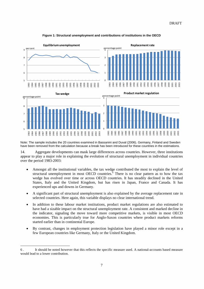
Figure 1: Structural unemployment and contributions of institutions in the OECD

Note: The sample includes the 20 countries examined in Bassanini and Duval (2006). Germany, Finland and Sweden have been removed from the calculation because a break has been introduced for these countries in the estimations.

14. Aggregate developments can mask large differences across countries. However, three institutions

appear to play a major role in explaining the evolution of structural unemployment in individual countries

over the period 1983-2003:

Amongst all the institutional variables, the tax wedge contributed the most to explain the level of

structural unemployment in most OECD countries.6 There is no clear pattern as to how the tax

wedge has evolved over time or across OECD countries. It has steadily declined in the United

States, Italy and the United Kingdom, but has risen in Japan, France and Canada. It has

experienced ups and downs in Germany.

A significant part of structural unemployment is also explained by the average replacement rate in

selected countries. Here again, this variable displays no clear international trend.

In addition to these labour market institutions, product market regulations are also estimated to

have had a sizable impact on the structural unemployment rate. A consistent and marked decline in

the indicator, signaling the move toward more competitive markets, is visible in most OECD

economies. This is particularly true for Anglo-Saxon countries where product markets reforms

started earlier than in continental Europe.

By contrast, changes in employment protection legislation have played a minor role except in a

few European countries like Germany, Italy or the United Kingdom.

6 . It should be noted however that this reflects the specific measure used. A national-accounts based measure

would lead to a lower contribution.

5

6

7

8

9

19

83

19

84

19

85

19

86

19

87

19

88

19

89

19

90

19

91

19

92

19

93

19

94

19

95

19

96

19

97

19

98

19

99

20

00

20

01

20

02

20

03

Equilibrium unemploymentper cent

0

1

2

3

4

19

83

19

84

19

85

19

86

19

87

19

88

19

89

19

90

19

91

19

92

19

93

19

94

19

95

19

96

19

97

19

98

19

99

20

00

20

01

20

02

20

03

Replacement ratepercentage point

5

6

7

8

9

19

83

19

84

19

85

19

86

19

87

19

88

19

89

19

90

19

91

19

92

19

93

19

94

19

95

19

96

19

97

19

98

19

99

20

00

20

01

20

02

20

03

Tax wedgepercentage point

0

1

2

3

4

19

83

19

84

19

85

19

86

19

87

19

88

19

89

19

90

19

91

19

92

19

93

19

94

19

95

19

96

19

97

19

98

19

99

20

00

20

01

20

02

20

03

Product market regulationpercentage point

DRAFT

8

Figure 2: Correlation between the change in institutions and cumulative changes in the NAIRU

-0.1

-0.05

0

0.05

0.1

0.15

lag

1

lag

2

lag

3

lag

4

lag

5

lag

6

lag

7

lag

8

lag

9

lag

10

Average replacement ratio

years

-0.1

-0.05

0

0.05

0.1

0.15

lag

1

lag

2

lag

3

lag

4

lag

5

lag

6

lag

7

lag

8

lag

9

lag

10

Tax wedge

years

-0.1

-0.05

0

0.05

0.1

0.15

lag

1

lag

2

lag

3

lag

4

lag

5

lag

6

lag

7

lag

8

lag

9

lag

10

EPL

years

-0.1

-0.05

0

0.05

0.1

0.15

lag

1

lag

2

lag

3

lag

4

lag

5

lag

6

lag

7

lag

8

lag

9

lag

10

Product market regulation

years

-0.1

-0.05

0

0.05

0.1

0.15

lag

1

lag

2

lag

3

lag

4

lag

5

lag

6

lag

7

lag

8

lag

9

lag

10

EPL Regular

years

-0.1

-0.05

0

0.05

0.1

0.15

lag

1

lag

2

lag

3

lag

4

lag

5

lag

6

lag

7

lag

8

lag

9

lag

10

EPL Temporary

years

DRAFT

9

15. In order to give some insights on the adjustment process and the lagged effects of structural

reforms, correlations have been computed between the cumulative increase in the NAIRU between time t-i

and t and the change in the institution at time t-i (Figure 2).7 It appears that:

A change in institutions, in particular the tax wedge, the replacement ratio and product market

regulations, has a gradual effect on the NAIRU changes. The impact peaks after 5 to 10 years,

depending on the measure considered.

In the short-term the maximum correlation is obtained for the tax wedge and product market

regulations and is significant.8 The cumulative impact of a change in the tax wedge on the change

in the NAIRU rises over the first four years and then gradually diminishes, ending up close to zero

after 7 years. By contrast, product market regulations continue to display a significant though

small effect over 10 years.

The correlation between the change in the average replacement ratio and the change in the NAIRU

is negligible in the short term but gradually increases over time, implying very long lags in the

adjustment process. The correlation becomes significant only after a decade or so.

The correlation between a change in employment protection legislation (EPL) and a change in the

NAIRU remains insignificant over a ten-year period. This result holds for both temporary and

regular contracts.

16. These results are subject to a number of caveats. The correlations have been computed using a

small number of observations and may be distorted by the presence of other, omitted determinants of

structural unemployment. Moreover, Granger tests fail to provide robust evidence of causality between

institutions and NAIRUs across countries.9

17. Overall, these results suggest that the impact of reforms is likely to be gradual and spread out

over many years. Structural reforms can lead to a costly reallocation of resources, so that efficiency

gains may take time to materialise. The following sections seek to provide additional information on the

shape and speed of adjustment following selected labour market reforms.

4. Labour and product market rigidities and adjustment speed

18. A number of previous studies have suggested that interactions between different areas of

structural reforms are crucial for their aggregate economic impact: returns of doing one reform would be

enhanced when other reforms have already been implemented (Bassanini and Duval, 2006). Political

economy considerations also indicate that injecting competition in product markets eases opposition and

political resistance to labour market reforms, because product market reforms tend to lower the rents to be

redistributed between unions and firms (Blanchard and Giavazzi, 2003). The objective of this section is to

examine whether policy complementarities may also affect short-term adjustment to structural reforms, in

particular to what extent product and labour market flexibility accelerates the pass-through of subsequent

reforms.

7. In this subsection, OECD Economic Outlook NAIRUs rather than structural unemployment rates have

been used as the latter are by construction correlated with institutions. NAIRUs and structural unemployments usually

display similar trends in OECD countries but some levels differences can be observed for some countries.

8. A simple rule of thumb derived from regression analysis is that the correlation is significant when it

exceeds 0.1.

9. Results are available on request.

DRAFT

10

Employment adjustment costs have a moderate impact on real adjustment…

19. To examine the impact of existing hiring and firing costs on the speed of adjustment to new

labour market reforms, a one percentage point income tax cut in the euro area was simulated using the

DGE model presented in Box 2. In this model, hiring and firing costs are modeled through quadratic

adjustment costs and provide firms with an incentive to smooth supply adjustment over time.10

These costs

delay the transition of employment, production and consumption to the new steady state in the aftermath of

structural reforms.

20. The introduction of adjustment costs to proxy nominal and real rigidities is standard in the DGE

literature (e.g. Coenen et al., 2007; Grenouilleau et al., 2007; Campolmi and Faia, 2007; Moyen and

Sahuc, 2005) but a number of specifications has been used. Quadratic cost specifications allow the quantity

and price adjustments to be smoothed over time. Other functional forms, such as linear or even declining

marginal adjustment costs, imply much faster and more abrupt adjustment paths. From this perspective, the

quadratic specification of adjustment costs in this paper provides an upper bound for the adjustment

duration and the impact of adjustment costs on the reform pass-through. In addition, micro level research

gives information on asymmetric cost patterns, with either hiring or firing being more costly for firms

depending on the regulatory circumstances. Such asymmetric behaviour is less relevant however in the

context of this paper, because the simulations focus on adjustment after reforms that lead to higher

employment and not on adjustment within the business cycle.

21. Substituting lower US adjustment costs for higher euro area ones would accelerate adjustment

towards the new equilibrium (Figure 3). Similar results obtain for a cut in the benefit replacement ratio or

in employer social security contributions (see Annex 4, Figures A.4.1 and A.4.2). Overall, the gain in

production and consumption adjustment speed from lower employment costs seems nevertheless very

modest, amounting to no more than two or three quarters. The differences are more marked with regard to

inflation as cuts in the income tax rate, benefit replacement rates or employer social security contributions

all indirectly or directly reduce production costs. The cuts initially have a slightly deflationary effect,

which in turn triggers an expansionary monetary reaction. Simulations suggest that if the euro area would

have had US employment adjustment costs, price cuts could be more pronounced implying a stronger

though temporary decline in real wages in the transition process. Introducing heterogeneity in the form of

liquidity-constrained consumers within the household sector, if anything, lowers the impact of employment

adjustment costs on the adjustment process (see section 5).

10. See Cahuc and Zylberberg (2004) for an excellent overview on labour adjustment costs.

DRAFT

11

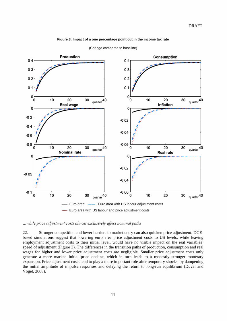
Figure 3: Impact of a one percentage point cut in the income tax rate

(Change compared to baseline)

––– Euro area ―― Euro area with US labour adjustment costs

- Euro area with US labour and price adjustment costs

…while price adjustment costs almost exclusively affect nominal paths

22. Stronger competition and lower barriers to market entry can also quicken price adjustment. DGE-

based simulations suggest that lowering euro area price adjustment costs to US levels, while leaving

employment adjustment costs to their initial level, would have no visible impact on the real variables’

speed of adjustment (Figure 3). The differences in the transition paths of production, consumption and real

wages for higher and lower price adjustment costs are negligible. Smaller price adjustment costs only

generate a more marked initial price decline, which in turn leads to a modestly stronger monetary

expansion. Price adjustment costs tend to play a more important role after temporary shocks, by dampening

the initial amplitude of impulse responses and delaying the return to long-run equilibrium (Duval and

Vogel, 2008).

DRAFT

12

Figure 4: Impact of a one-percentage point income tax cut in a search-and-matching framework



- Euro area US labour and price adjustment costs

23. This result also holds when the labour market is modelled through an alternative search and

matching framework (see Annex 3 for details). In this case, reduced employment adjustment costs would

have fairly limited effects on the adjustment speed of production and consumption, while the contribution

of lower price adjustment costs is negligible. Differences are more pronounced with regard to price, real

wage and interest rate patterns. Labour supply increases faster than labour demand in the presence of

adjustment costs and frictional unemployment. The mismatch between labour supply and demand exerts

downward pressure on real wages, production costs and prices. In addition, higher employment adjustment

DRAFT

13

costs put additional pressure on real wages.11

As these effects are quantitatively strong, the economy will

experience stronger monetary accommodation than in the simulation based on the standard DGE model.

24. The small impact of price and employment adjustment costs on the pace of adjustment is also

confirmed by simulations using neo-Keynesian models for the United States and the euro area (see Annex

5). Indeed, in the absence of an endogenous monetary policy reaction, the euro area and the United States

are found to adjust to a shock on the NAIRU at a similar pace at least in the short-term, even though the

United States displays greater wage flexibility than the euro area.

5. Financial markets and adjustment speed

25. Flexible and forward-looking financial markets can affect the adjustment speed to structural

reforms. The United States deregulated its product and financial markets in the 1980s. Reforms have been

more recent and less comprehensive within the euro area, even though major progress has been recently

accomplished. Past reforms have increased the responsiveness of the economy to policy impulses and

strengthened the direct impact of interest rates on financial decisions of both firms and households

(Angeloni et al., 2003; Edey and Hviding, 1995; Mishkin, 2007).

26. Full access to credit allows firms to adjust their investment to their desired level and is thus

likely to fasten adjustments to structural reform. In particular, deep venture capital markets facilitate the

creation of firms and are found to explain differences in labour market performance between Anglo-saxon

economies and Continental Europe (Belke and Fehn, 2001; Acemoglu, 2001).

27. Financial sector reforms in the United States in the 1970s and 1980s are also estimated to

have reduced the share of liquidity-constrained households (Sefton and In’t Veld, 1999). The subsequent

liberalisation of financial markets in the euro area is also expected to have had similar effects, though it is

hard to quantify its precise magnitude. But the effect of easing households’ liquidity constraints on

adjustment speeds is a priori an empirical question. On the one hand, more households optimise their

consumption decisions and smooth income over time. On the other hand, habit persistence in these

households’ consumption behaviour is likely to slow the speed of adjustment.

28. This question can be examined by enriching the DGE model with a heterogeneous household

sector. Some households have full access to financial markets, while others get limited or no access to

financial markets and can only consume their disposable labour income at each period. A one-percentage

point income tax cut is then simulated under three alternatives: all households have full access to financial

markets; 25% of the households are liquidity constrained; and 75% are liquidity constrained. Although the

main differences are on the long term and reflect differences in utility functions between the two groups of

households, changes to short-term adjustments can also be observed on inflation and monetary policy

reaction (Figure 5). As the magnitude of the policy response varies with the share of liquidity-constrained

households, the final effect on the pace of adjustment of real variables is negligible in the model. By

omitting capital adjustments, these simulations may nevertheless underestimate the overall effect of

liquidity constraints.

11. The higher adjustment costs result from adjustment costs relating to gross instead of net flows of

labour in the search-and-matching extension. Each period a certain and fixed share of workers loses or quits a job for

new positions or unemployment. Consequently, gross flows in and out of employment differ from net flows and are

usually higher than the latter. Contrary to the baseline model, labour adjustment costs also affect the steady state

production and consumption level in the search-and-matching framework. As there are separations in each period,

positive adjustment costs will even accrue in the steady state, reducing the level of consumption and equilibrium

employment.

DRAFT

14

Figure 5: Impact of a one percentage point income tax cut under alternative share of liquidity-constrained households in the euro area


Share of liquidity-constrained consumers: ––– 0% ―― 25% 75%

6. Interaction with monetary policy

29. The implementation of labour market reforms has usually a significant macroeconomic impact in

the short term and can call for a policy reaction. In turn, monetary policy decisions can affect the transition

speed in the aftermath of structural reforms, though to a different degree across OECD countries,

depending on the strength of the transmission channels and on the sensitivity of policy rates to output and

inflation. Indeed, demand expansion reduces the transition costs of reform policies and lowers

unemployment stemming from the required restructuring of particular industries. From a political economy

point of view, the ability and willingness of central bankers to accommodate structural reforms may reduce

transitory costs and political opposition and thereby facilitate implementation.

DRAFT

15

Figure 6: Effect of monetary policy on adjustment to a 1 percentage point NAIRU decline

Effect on real GDP

(change compared to baseline)

Effect on inflation

(change compared to baseline)

-0.2

0.0

0.2

0.4

0.6

0.8

1.0

0 10 20 30 40 50 60 70 80

United States

without monetary policy reactionwith monetary policy reaction

quarters

%

0

0.2

0.4

0.6

0.8

1

0 10 20 30 40 50 60 70 80

France

without monetary policy reaction

with monetary policy reaction

quarters

%

-0.2

0

0.2

0.4

0.6

0.8

0 10 20 30 40 50 60 70 80

Euro area



quarters

%

-0.3

-0.2

-0.1

0

0 10 20 30 40 50 60 70 80United States



quarters

%

-1.2

-1

-0.8

-0.6

-0.4

-0.2

0

0 10 20 30 40 50 60 70 80

Euro area



quarters

%

-0.6

-0.4

-0.2

0

0 10 20 30 40 50 60 70 80

France

without monetary policy reactionwith monetary policy reaction

quarters

%

DRAFT

16

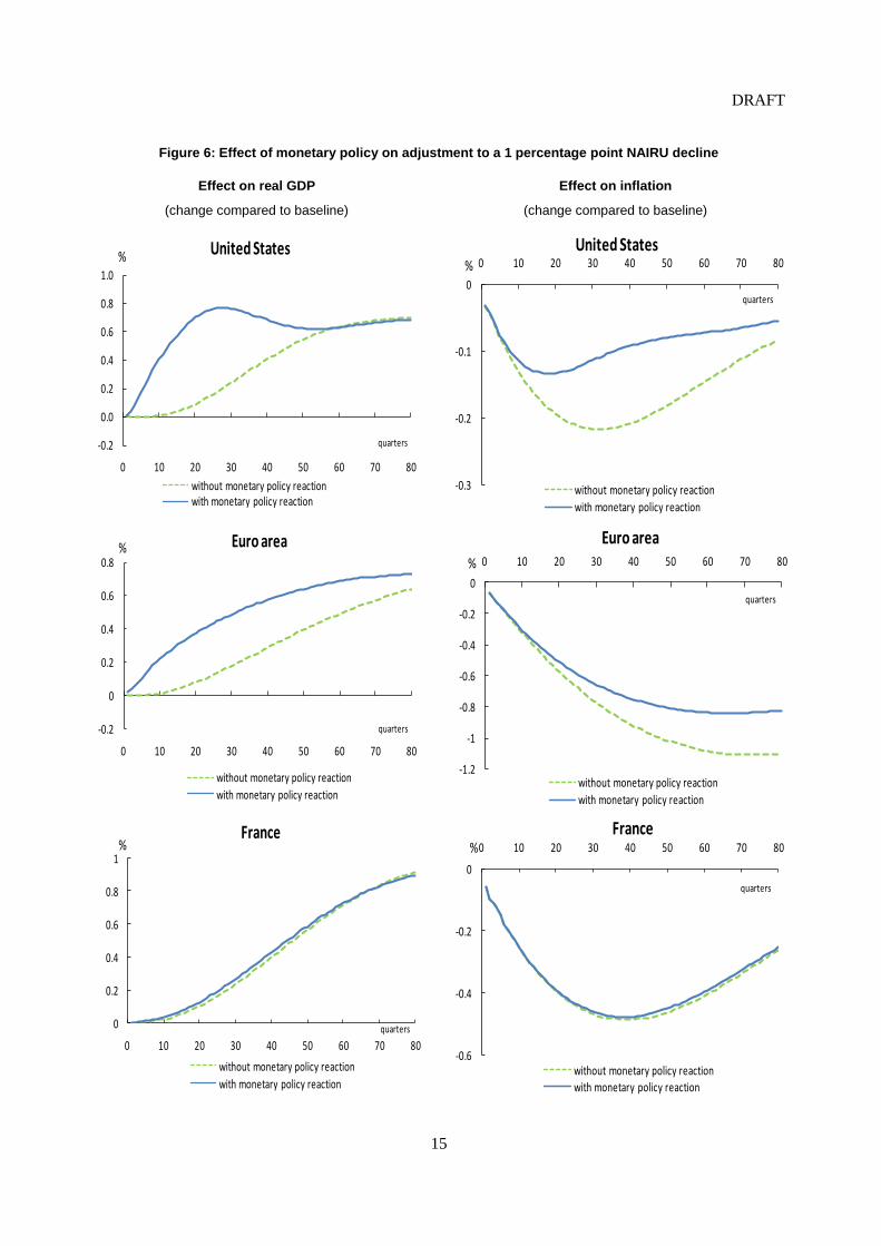
30. The interaction between structural reforms and monetary policy can be illustrated by simulating a

one percentage-point decline in the NAIRU, using the neo-Keynesian small models described in Box 1. In

the absence of a monetary policy reaction, a decline in the NAIRU generates disinflationary effects, while

output and unemployment gaps are building up. The introduction of monetary policy, in the form of a

Taylor rule with equal weights on output and inflation, dampens the disinflationary effect and accelerates

the move to the new long-term equilibrium (Figure 6).

31. Expected gains from monetary policy reaction are estimated to be negligible for individual euro

area economies. As the ECB focuses on aggregate euro area output and inflation, any monetary reaction to

a reform implemented in an individual European country is improbable unless there is a coordinated effort

to reform labour markets in a sufficient number of euro area countries. This holds for small but also large

euro area economies. For instance, a domestic reform lowering the NAIRU by one percentage point in

France, which accounts for about 20% of euro area GDP, would elicit almost no monetary policy reaction.

Figure 7: Impact of a one percentage point decline in the NAIRU under alternative monetary policy reactions

32. The contrast between the two sides of the Atlantic reflects differences in monetary transmission

channels as modeled in the neo-Keynesian models. Demand components, especially business investment,

are found to be more sensitive to real interest rates in the United States than in the euro area. Consequently,

the United States would adjust much faster to the new steady state than the euro area in the presence of

monetary policy reaction.12

33. Modifying the monetary policy reaction function can alter the pace of adjustment for the euro

area. The impact of adopting a different monetary policy rule has been examined by simulating a cut in the

NAIRU in the euro area under different policy reactions: a Taylor rule with equal weights on inflation and

the output gap; a Taylor rule with a stronger weight on inflation; and pure inflation targeting, with no

12. Because consumption equations have not been estimated over the same period in the United States and

the euro area, the traditional result that consumption is more sensitive to interest rates in the United States than in the

euro area does not apply in this simulation. Hence, differences in the adjustment process between the United States

and the euro area in the presence of monetary reaction may be underestimated.

0

0.2

0.4

0.6

0.8

1

1.2

0 10 20 30 40 50 60 70 80

Euro area real GDP(difference from baseline)

Taylor rule (0.5, 0.5) Inflation targeting

Taylor rule (0.2, 0.8) US real GDP with Taylor rule (0.5, 0.5)

quarters

%

DRAFT

17

weight on the output gap. Increasing the weight of inflation in the monetary reaction function appears to

slow the adjustment in the very short term but quicken it thereafter. As a result, the economy reaches its

long-term equilibrium much earlier, but with some overshooting (Figure 7). Even in the case of pure

inflation targeting, the adjustment speed would nevertheless remain slower in the euro area than in the

United States. Interest rate persistence, which implies that central banks are reluctant to move the policy

rate too rapidly to limit output volatility, can slow the adjustment to structural reforms. However, both

DGE and neo-Keynesian-based simulations suggest that interest rate persistence has to be very high (with a

weight close to unity) to have visible effects on adjustment of real variables.

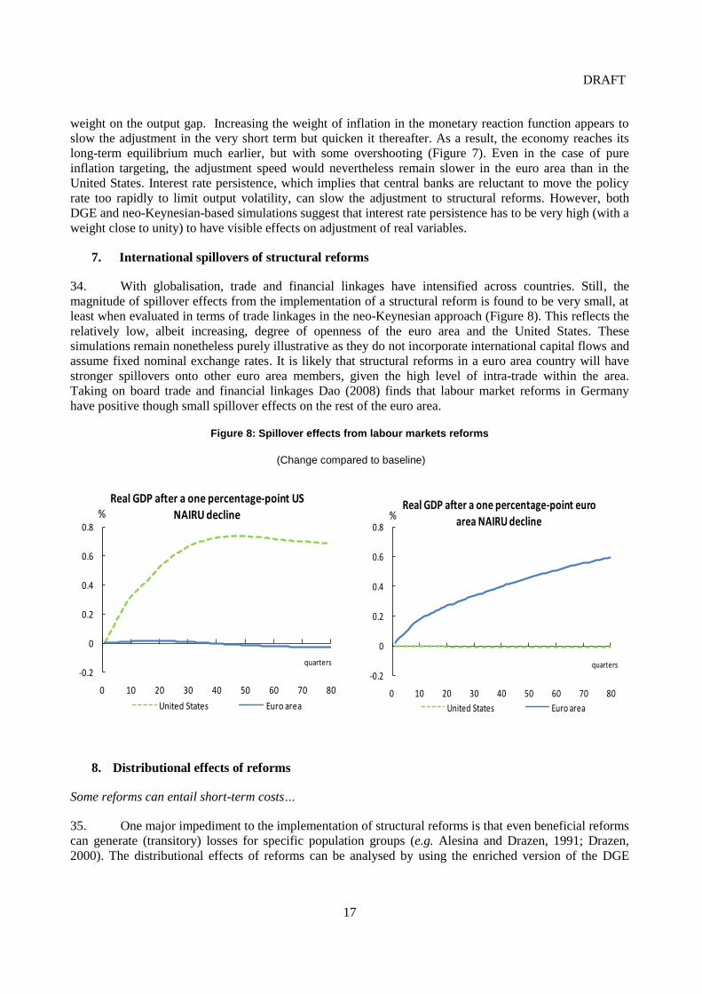
7. International spillovers of structural reforms

34. With globalisation, trade and financial linkages have intensified across countries. Still, the

magnitude of spillover effects from the implementation of a structural reform is found to be very small, at

least when evaluated in terms of trade linkages in the neo-Keynesian approach (Figure 8). This reflects the

relatively low, albeit increasing, degree of openness of the euro area and the United States. These

simulations remain nonetheless purely illustrative as they do not incorporate international capital flows and

assume fixed nominal exchange rates. It is likely that structural reforms in a euro area country will have

stronger spillovers onto other euro area members, given the high level of intra-trade within the area.

Taking on board trade and financial linkages Dao (2008) finds that labour market reforms in Germany

have positive though small spillover effects on the rest of the euro area.

Figure 8: Spillover effects from labour markets reforms


8. Distributional effects of reforms

Some reforms can entail short-term costs…

35. One major impediment to the implementation of structural reforms is that even beneficial reforms

can generate (transitory) losses for specific population groups (e.g. Alesina and Drazen, 1991; Drazen,

2000). The distributional effects of reforms can be analysed by using the enriched version of the DGE

-0.2

0

0.2

0.4

0.6

0.8

0 10 20 30 40 50 60 70 80

Real GDP after a one percentage-point US NAIRU decline

United States Euro area

quarters

%

-0.2

0

0.2

0.4

0.6

0.8

0 10 20 30 40 50 60 70 80

Real GDP after a one percentage-point euro area NAIRU decline

United States Euro area

quarters

%

DRAFT

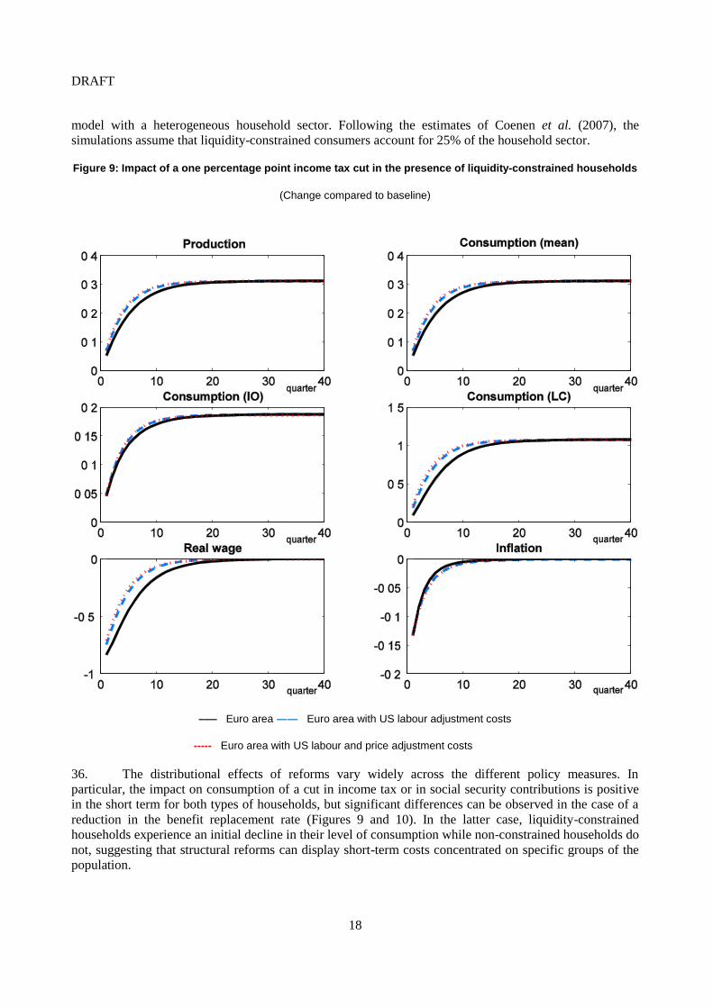
18

model with a heterogeneous household sector. Following the estimates of Coenen et al. (2007), the

simulations assume that liquidity-constrained consumers account for 25% of the household sector.

Figure 9: Impact of a one percentage point income tax cut in the presence of liquidity-constrained households



- Euro area with US labour and price adjustment costs

36. The distributional effects of reforms vary widely across the different policy measures. In

particular, the impact on consumption of a cut in income tax or in social security contributions is positive

in the short term for both types of households, but significant differences can be observed in the case of a

reduction in the benefit replacement rate (Figures 9 and 10). In the latter case, liquidity-constrained

households experience an initial decline in their level of consumption while non-constrained households do

not, suggesting that structural reforms can display short-term costs concentrated on specific groups of the

population.

DRAFT

19

37.

Figure 10: Impact of a one percentage point cut in the benefit replacement rate in the presence of liquidity-constrained households



Euro area with US labour and price adjustment costs

38. Employment adjustment costs have temporary but moderate effects on the distribution of income

and consumption gains between households. Reducing euro area employment adjustment costs to their US

levels has virtually no effect on the consumption path of intertemporally optimising households but a

DRAFT

20

significant impact on liquidity-constrained households.13

Indeed, it reduces the amplitude of the decline in

real wages during the transition, so that the consumption of liquidity-constrained agents is higher.

39. Price adjustment costs are found to have a marginal impact on real adjustment after structural

reforms, the main exception being in the case of a benefit replacement rate cut (Figure 8). The reduction of

the reservation wage puts downward pressure on real wages and lowers production costs. The faster the

reaction of prices to lower production costs, the weaker the reaction of real wages and the decline in

consumption from liquidity-constrained households.

40. The impact of these costs varies across policy measures (Annex 4 Figures A.4.5). Lower

employment adjustment costs accelerate the adjustment of real wages and liquidity-constrained

consumption after an income tax rate cut or a cut in employer social security contributions. However, the

difference is more pronounced after a benefit replacement rate reduction, as liquidity-constrained

consumers initially lose income. Lower adjustment costs attenuate and shorten the temporary real wage

decline and the transitory real consumption loss for liquidity-constrained households.

…but budgetary compensation schemes can reduce these costs

41. The introduction of a fiscal rule to balance the government budget after the implementation of

structural reforms can have a marked impact on the short-term adjustment and the long-run distribution of

efficiency gains (Figure 11). Under a deficit-neutral reform, the government budget is balanced at each

point in time, assuming for simplicity, the availability of lump-sum taxes and transfers. The baseline

scenario assumes that liquidity-constrained households proportionately share the fiscal burden, after a tax

cut or the reduction in social security contributions, or the fiscal gains from a reduction in the benefit

replacement rate. Under an alternative scenario, the fiscal burden or gain is entirely shifted to the

intertemporally optimising households. Lump-sum measures offset the wealth effect of reforms without

introducing further substitution effects.14

Relying on distortionary taxation and demand components

instead would affect incentives and either reinforce or soften the initial impact of the reform.

42. Shifting the entire fiscal burden of an income tax cut or a reduction in employer social security

contributions to intertemporally optimising households diminishes the latters’ gains from structural

reforms. By contrast, liquidity-constrained consumers experience an increase in disposable income and

consumption. Depriving liquidity-constrained households from the fiscal gains from lower unemployment

transfers would have the opposite effect. Liquidity-constrained households would lose in net wealth terms,

while optimising consumers would gain compared to the baseline redistribution scheme, where costs are

shared between the two types of households.

43. A budget consolidation scheme would affect not only the relative long-term position of the two

types of consumers, but also aggregate production and consumption in the long run. Exempting liquidity-

constrained consumers from fiscal consolidation reduces aggregate output (Figure 11), while excluding

them from the redistribution of fiscal surpluses would moderately raise long-run production (Figure A.4.6).

These effects stem from the modelling of the labour market and reflect mostly the assumption of

diminishing marginal utility of income. Liquidity-constrained households do not receive profits and

dividends from firms and thus consume less than unconstrained households in the steady state. The

13. We assume a budget-neutral policy that immediately offsets the wealth effect of fiscal measures by

proportionate lump-sum transfers and where each household type receives a proportionate share of these transfers.

The subsequent section discusses the impact of the wealth effect on the impulse responses.

14. As the intertemporal optimisers operate under an infinite planning horizon the time structure of budget

consolidation does not affect private sector behaviour in this case. Budget balancing may even only occur in the

distant future.

DRAFT

21

exemption from fiscal consolidation raises liquidity-constrained consumers’ disposable income and

consumption. Given the decreasing marginal utility of consumption, labour supply declines and wage

claims rise, reducing equilibrium employment and production. Excluding liquidity-constrained households

from the redistribution of fiscal gains reduces their disposable income and leads to wage moderation and

higher production. As structural reforms have a permanent budgetary impact in the model these income

effects are also long-lasting.

Figure 11: Impact of a one percentage point cut in income tax with budget balance rule


––– Contribution from both types of households ―― No contribution from liquidity-constrained households

8. Conclusions

44. Economic adjustment to structural reforms is a gradual process. Drawing on various

methodologies – descriptive analysis, macro-economic neo-Keynesian models, and a micro-founded

dynamic general equilibrium model – this paper investigates the lag between the implementation of

DRAFT

22

reforms and their economic effects, the impact of markets rigidities, the role of monetary policy in the

transition period and questions of distributional effects.

45. The complementarities of these three different approaches motivate their combined use. The

descriptive part seeks to draw conclusions from past OECD country experience in structural reforms. But,

it strongly relies on data that often lack reliability and timeliness. Neo-Keynesian models have the

advantage of using estimated behavioural equations for the euro area and the United States. However, the

effect of some relevant institutions can be included only very indirectly, using off-model information, and

this approach is subject to the Lucas critique. Finally, the micro-founded DGE model illustrates the

respective transmission channels of several types of structural reforms (tax policy, social security schemes,

competition policy). However, the introduction of employment and price adjustment costs as well as habit

persistence in consumption in the model is insufficient to generate substantial cross-country heterogeneity

in the adjustment speed. Methodological eclecticism is also a way to test the robustness of findings, where

possible. In this regard, it is reassuring that the results of the paper for which robustness could be tested

hold independently from the methodological approach adopted (e.g. limited role of price adjustment costs

in the speed of adjustment to reforms).

46. The paper leaves ample room for extensions in particular on the modelling side. First, the

introduction of explicit households’ accounts would allow simulating explicitly the impact of tax reforms

in the neo-Keynesian framework. Second, one could examine whether monetary policy has become more

or less important over time in accommodating structural reforms by examining whether the impact of

interest rates on the main behavioural equations has been modified in recent years. Third, the DGE model

could be substantially refined by introducing additional frictions such as wage rigidities or capital

adjustment costs, although this would considerably increase the complexity of the framework. In the same

vein, the work could be extended to a framework with a multi-factor production function and instead of

calibrating the parameters, Bayesian techniques could be used to estimate DGE models for different

countries.

DRAFT

23

REFERENCES

Acemoglu, D. (2001), “Credit Market Imperfections and persistent unemployment”, European

Economic Review, No. 45, pp. 665-679.

Alesina, A. and A. Drazen (1991), “Why Are Stabilizations Delayed?”, American Economic Review,

Vol. 81, No. 5, pp. 1170-1188.

Altissimo, F., M. Ehrmann and F. Smets (2006), “Inflation Persistence and Price-Setting Behaviour in

the Euro Area: A Summary of the IPN Evidence”, ECB Occasional Papers, No. 46.

Angeloni, I., A. Kashyap and B. Mojon (eds), 2003, Monetary Policy Transmission in the Euro Area,

Cambridge University Press.

Amato, J. and T. Laubach (2003), “Rule-of-Thumb Behaviour and Monetary Policy”, European

Economic Review, Vol. 47, No. 5, pp. 791-831.

Arpaia, A., W. Roeger, J. Varga, J. in’t Veld, I. Grolo and P. Wobst (2007), “Quantitative Assessment

of Structural Reforms: Modelling the Lisbon Strategy”, European Economy Economic Papers, No. 282.

Bassanini, A. and R. Duval (2006), “Employment Patterns in OECD Countries: Reassessing the Role

of Policies and Institutions”, OECD Economics Department Working Papers, No. 486.

Batini N., P. N’Diaye and A. Rebucci (2005), “The Domestic and Global Impact of Japan’s Policies

for Growth”, IMF Working Papers, No. 05/209.

Bean, C. (1998), “The Interaction of Aggregate Demand Policies and Labour Market Reforms”,

Swedish Economic Policy Review, Vol. 5, No. 2, pp. 353-382.

Belot, M. and J. van Ours (2001), “Unemployment and Labour Market Institutions: An Empirical

Analysis”, Journal of the Japanese and International Economies, Vol. 15, No. 4, pp. 403-418.

Berke, A., and R. Fehn (2001), “Institutions and Structural Unemployment: Do Capital-Market

Imperfections Matter?”, CESinfo Working Paper, No. 504.

Bils, M. and P. Klenow (2004), “Some Evidence on the Importance of Sticky Prices”, Journal of

Political Economy, Vol. 112, No. 5, pp. 947-984.

Blanchard, O. and F. Giavazzi (2003), “Macroeconomic Effects of Regulation and Deregulation on

Goods and Labour Markets”, Quarterly Journal of Economics, Vol. 118, No. 3, pp. 879-907.

Cahuc, P. and A. Zylberberg (2004), Labour Economics, MIT Press, Cambridge, Mass.

Campolmi, A. and E. Faia (2006), “Cyclical Inflation Divergence and Different Labor Market

Institutions in the EMU”, ECB Working Papers, No. 619.

Christopoulou, R. and P. Vermeulen (2008), “Markups in the Euro Area and the US over the Period

1981-2004”, ECB Working Papers, No. 856.

DRAFT

24

Coenen, G., P. McAdam and R. Straub (2007), “Tax Reform and Labour-Market Performance in the

Euro Area: A Simulation-Based Analysis Using the New Area-Wide Model”, ECB Working Papers, No.

747.

Dao, M. (2008), “International Spillover of Labour Market Reforms”, IMF Working Paper, No.

08/113.

Drazen, A. (2000), Political Economy in Macroeconomics, Princeton University Press, Princeton.

Dreger, C., M. Artís, R. Moreno, R. Ramos and J. Suriñach (2007), “Study on the Feasibility of a

Tool to Measure the Macroeconomic Impact of Structural Reforms”, European Economy Economic

Papers, No. 272.

Duval, R. and J. Elmeskov (2005), “The Effects of EMU on Structural Reforms in Labour and

Product Markets”, OECD Economics Department Working Papers, No. 438.

Duval, R., J. Elmeskov and L. Vogel (2007), “Structural Policies and Economic Resilience to

Shocks”, OECD Economics Department Working Papers, No. 567.

Duval, R. and L. Vogel (2008), “Oil Price Shocks, Rigidities and the Conduct of Monetary Policy:

Some Lessons from a New Keynesian Perspective”, OECD Economics Department Working Papers, No.

603.

Edey M. and K. Hviding (1995), “An Assessment of Financial Reforms in OECD Countries”, OECD

Economics Department Working Papers, No. 154.

Estevão, M. (2005), “Product Market Regulation and the Benefits of Wage Moderation”, IMF

Working Papers, No. 05/191.

Ernst, E., G. Gong, W. Semmler and L. Bukeviciute (2006), “Quantifying the Impact of Structural

Reforms”, ECB Working Papers, No. 666.

Everaert, L. and W. Schule (2006), “Structural Reforms in the Euro Area: Economic Impact and Role

of Synchronisation across Markets and Countries”, IMF Working Papers, No. 137.

Freeman, R. (1998), “War of Models: Which Labour Market Institutions for the 21st Century?”,

Labour Economics, Vol. 5, No. 1, pp. 1-24.

Fuhrer, J. (2000), “Habit Formation in Consumption and Its Implications for Monetary-Policy

Models”, American Economic Review, Vol. 90, No. 3, pp. 367-390.

Galí, J., D. Lopez-Salido and J. Vallés (2004), “Rule-of-Thumb Consumers and the Design of Interest

Rate Rules”, Journal of Money, Credit, and Banking, Vol. 36, No. 4, pp. 739-763.

Galí, J., D. López-Salido and J. Vallés (2007), “Understanding the Effects of Government Spending

on Consumption”, Journal of the European Economic Association, Vol. 5, No. 1, pp. 227-270.

Grenouilleau, D., M. Ratto and W. Roeger (2007), “Adjustment to Shocks: A Comparison between

the Euro Area and the US Using Estimated DSGE Models”, paper presented at the Workshop on Structural

Reforms and Economic Resilience, OECD, Paris, 14 June.

DRAFT

25

Hunt, B. and D. Laxton (2004), “Some Simulation Properties of the Major Euro Area Economies in

MULTIMOD”, Economic Modelling, Vol. 21, No. 5, pp. 759-783.

Inklaar, R. and M. Timmer (2006), “Resurgence of Employment Growth in the European Union: The

Role of Cycles and Labour Market Reforms”, Economics Letters, Vol. 91, No. 1, pp. 61-66.

Kilponen, J. and A. Ripatti (2006), “Labour and Product Market Reforms in General Equilibrium:

Simulation Results Using a DGE Model of the Finnish Economy”, Bank of Finland Research Discussion

Papers, No. 5/2006.

Mishkin, F. (2007), “Housing and the Monetary Transmission Mechanism”, NBER Working Papers,

No. 13518.

Moyen, S. and J.-G. Sahuc (2005), “Incorporating Labour Market Frictions into an Optimising-Based

Monetary Policy Model”, Economic Modelling, Vol. 22, No. 1, pp. 159-186.

Nicoletti, G. and S. Scarpetta (2005), “Product Market Reforms and Employment in OECD

Countries”, OECD Economics Department Working Paper, No. 472.

OECD (2007), Employment Outlook, OECD, Paris.

OECD (2008), Going for Growth, OECD , Paris.

Rotemberg, J. (1982), “Monopolistic Price Adjustment and Aggregate Output”, Review of Economic

Studies, Vol. 49, No. 4, pp. 517-531.

Sefton, J. and J. In't Veld (1999), “Consumption and Wealth: An International Comparison”, The

Manchester School, Vol. 67, No. 4, pp. 525-544.

Smets, F. and R. Wouters (2003), “An Estimated Dynamic Stochastic General Equilibrium Model of

the Euro Area”, Journal of the European Economic Association, Vol. 1, No. 5, pp. 1123-1175.

Smets, F. and R. Wouters (2005), “Comparing Shocks and Frictions in US and Euro Area Business

Cycles: A Bayesian DSGE Approach”, Journal of Applied Econometrics, Vol. 20, No. 2, pp. 161-183.

DRAFT

26

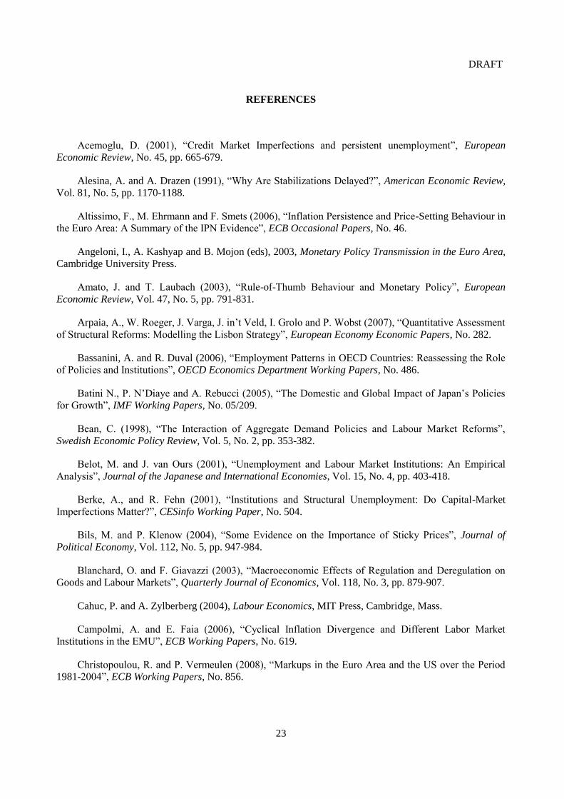
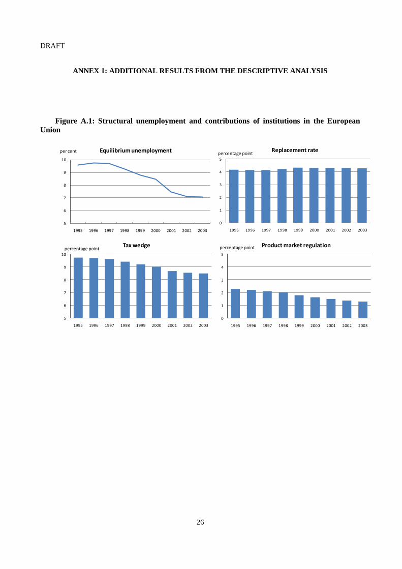
ANNEX 1: ADDITIONAL RESULTS FROM THE DESCRIPTIVE ANALYSIS

Figure A.1: Structural unemployment and contributions of institutions in the European

Union

5

6

7

8

9

10

1995 1996 1997 1998 1999 2000 2001 2002 2003


0

1

2

3

4

5

1995 1996 1997 1998 1999 2000 2001 2002 2003


5

6

7

8

9

10

1995 1996 1997 1998 1999 2000 2001 2002 2003


0

1

2

3

4

5

1995 1996 1997 1998 1999 2000 2001 2002 2003


DRAFT

27

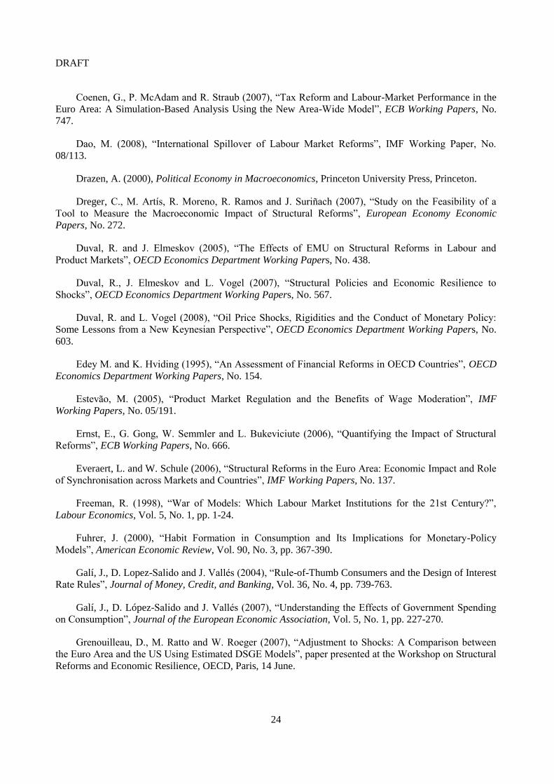
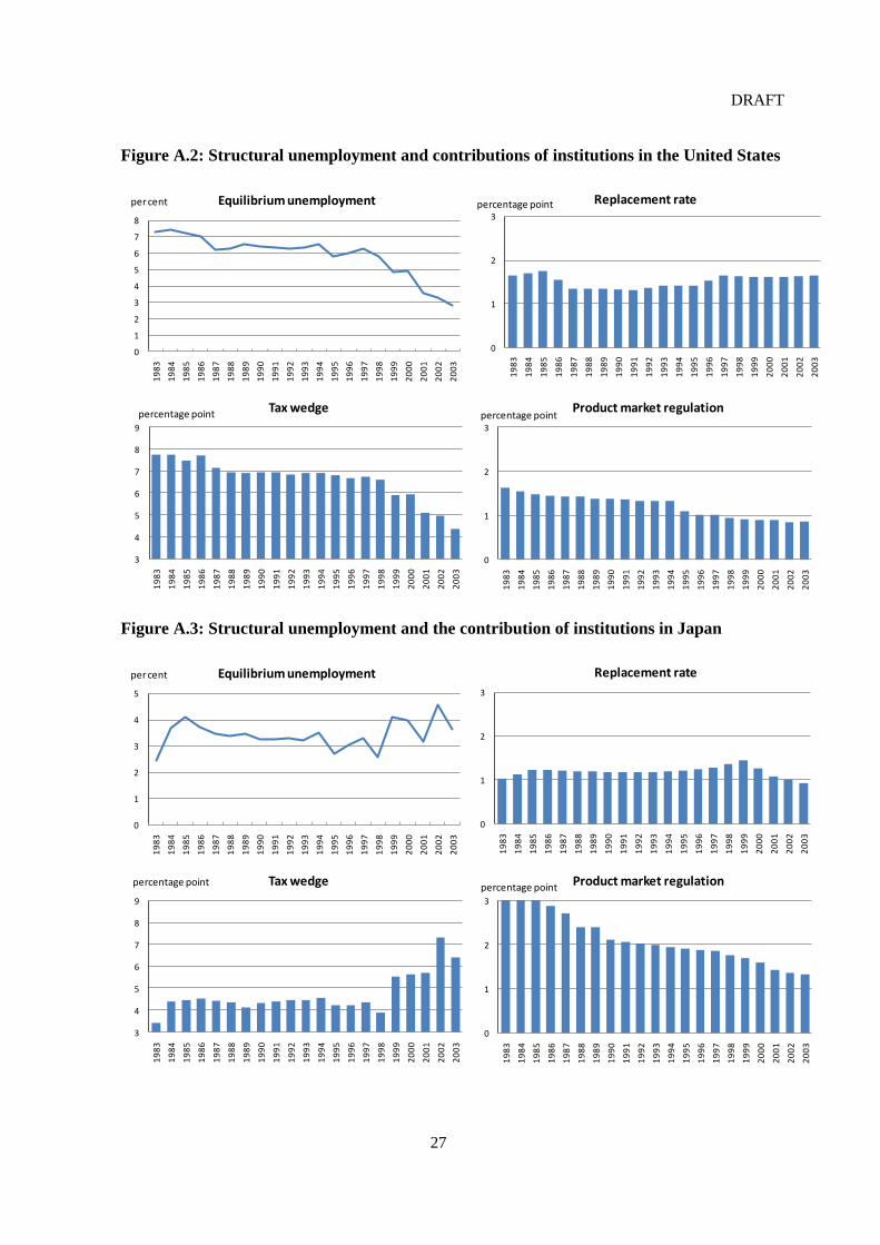
Figure A.2: Structural unemployment and contributions of institutions in the United States

Figure A.3: Structural unemployment and the contribution of institutions in Japan

0

1

2

3

4

5

6

7

8

19

83

19

84

19

85

19

86

19

87

19

88

19

89

19

90

19

91

19

92

19

93

19

94

19

95

19

96

19

97

19

98

19

99

20

00

20

01

20

02

20

03


0

1

2

3

19

83

19

84

19

85

19

86

19

87

19

88

19

89

19

90

19

91

19

92

19

93

19

94

19

95

19

96

19

97

19

98

19

99

20

00

20

01

20

02

20

03


3

4

5

6

7

8

9

19

83

19

84

19

85

19

86

19

87

19

88

19

89

19

90

19

91

19

92

19

93

19

94

19

95

19

96

19

97

19

98

19

99

20

00

20

01

20

02

20

03


0

1

2

3

19

83

19

84

19

85

19

86

19

87

19

88

19

89

19

90

19

91

19

92

19

93

19

94

19

95

19

96

19

97

19

98

19

99

20

00

20

01

20

02

20

03


0

1

2

3

4

5

19

83

19

84

19

85

19

86

19

87

19

88

19

89

19

90

19

91

19

92

19

93

19

94

19

95

19

96

19

97

19

98

19

99

20

00

20

01

20

02

20

03


0

1

2

3

19

83

19

84

19

85

19

86

19

87

19

88

19

89

19

90

19

91

19

92

19

93

19

94

19

95

19

96

19

97

19

98

19

99

20

00

20

01

20

02

20

03

Replacement rate

3

4

5

6

7

8

9

19

83

19

84

19

85

19

86

19

87

19

88

19

89

19

90

19

91

19

92

19

93

19

94

19

95

19

96

19

97

19

98

19

99

20

00

20

01

20

02

20

03


0

1

2

3

19

83

19

84

19

85

19

86

19

87

19

88

19

89

19

90

19

91

19

92

19

93

19

94

19

95

19

96

19

97

19

98

19

99

20

00

20

01

20

02

20

03


DRAFT

28

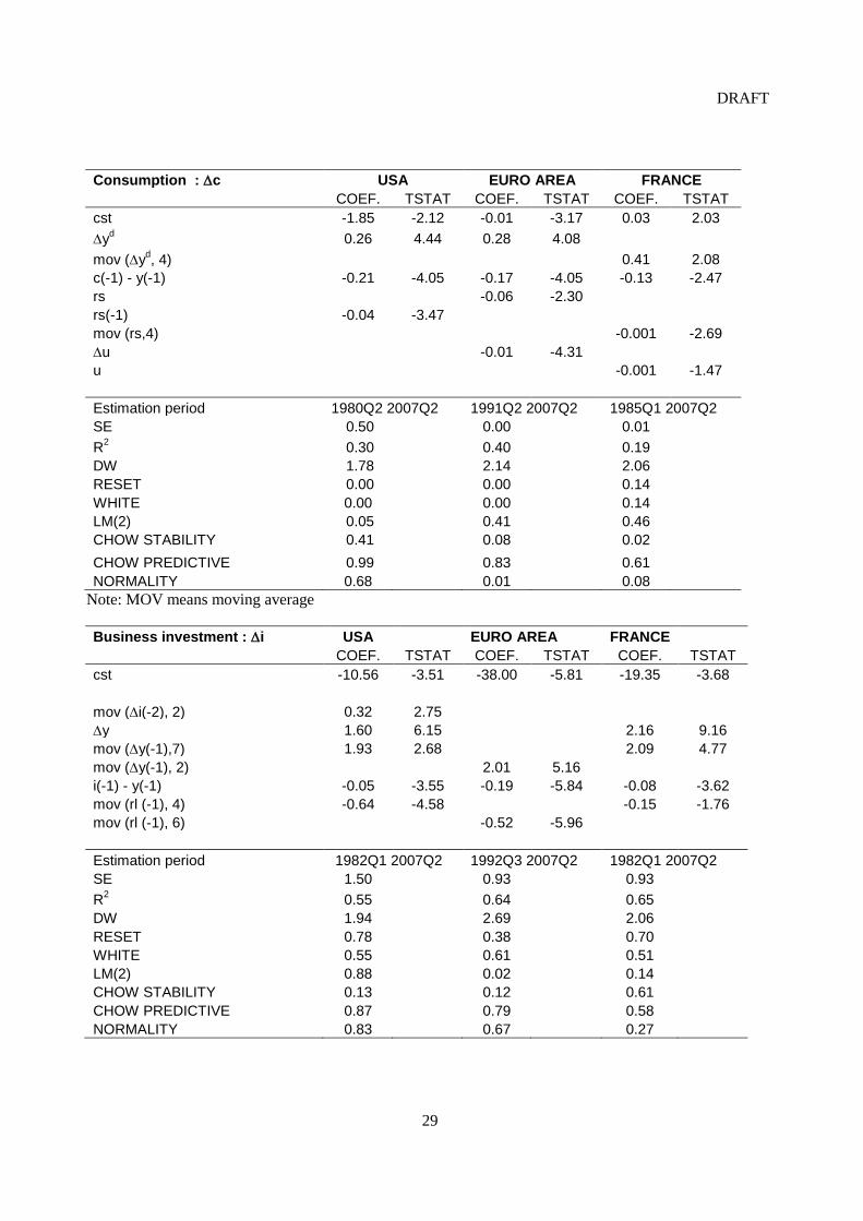
ANNEX 2: MAIN EQUATIONS OF THE NEO-KEYNESIAN MODELS

Equations are usually estimated in an error correction form using a general to specific approach.

Keys to variables

c private consumption

gap output gap

h hours

h* trend hours

i investment

ih housing investment

n employment

n* potential employment

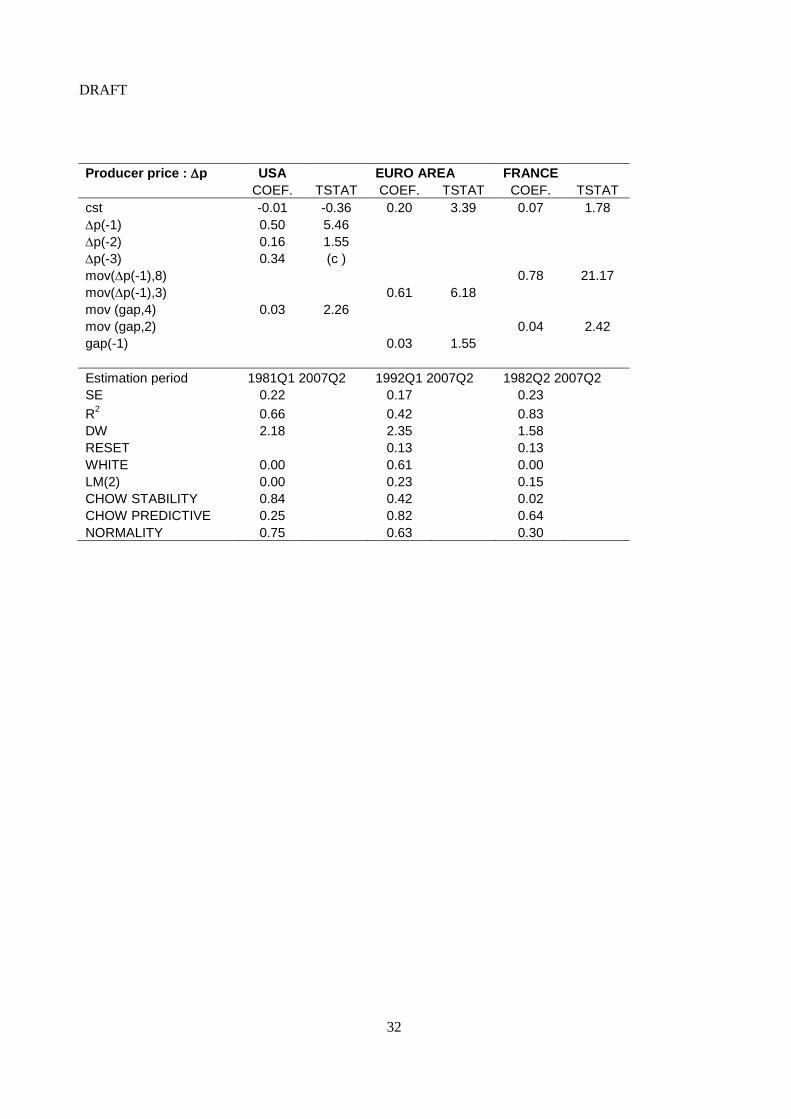
p production prices

pcore core consumer price

pih price of housing

pm import price all goods and services

rs short-term real interest rate

rl long-term real interest rate

u unemployment rate

ugap unemployment gap

w wage

yd household disposable income

y* potential output

Test

WHITE White heteroskedasticity test

LM(2) Breusch-Godfrey Serial Correlation LM Test - 2 lags

CHOW STABILITY Chow Breakpoint Test: 2000Q1

CHOW PREDICTIVE Chow Forecast Test: Forecast from 2006Q4 to 2007Q2

NORMALITY Jarque-Bera Normality test

DRAFT

29

Consumption : c USA EURO AREA FRANCE

COEF. TSTAT COEF. TSTAT COEF. TSTAT

cst -1.85 -2.12 -0.01 -3.17 0.03 2.03

yd 0.26 4.44 0.28 4.08

mov (yd, 4)

0.41 2.08

c(-1) - y(-1) -0.21 -4.05 -0.17 -4.05 -0.13 -2.47

rs

-0.06 -2.30 rs(-1) -0.04 -3.47

mov (rs,4)

-0.001 -2.69

u

-0.01 -4.31 u

-0.001 -1.47

Estimation period 1980Q2 2007Q2 1991Q2 2007Q2 1985Q1 2007Q2

SE 0.50

0.00

0.01 R

2 0.30

0.40

0.19

DW 1.78

2.14

2.06 RESET 0.00

0.00

0.14

WHITE 0.00

0.00

0.14 LM(2) 0.05

0.41

0.46

CHOW STABILITY 0.41

0.08

0.02 CHOW PREDICTIVE 0.99

0.83

0.61

NORMALITY 0.68 0.01 0.08

Note: MOV means moving average

Business investment : i USA EURO AREA FRANCE


cst -10.56 -3.51 -38.00 -5.81 -19.35 -3.68

mov (i(-2), 2) 0.32 2.75 y 1.60 6.15

2.16 9.16

mov (y(-1),7) 1.93 2.68

2.09 4.77

mov (y(-1), 2)

2.01 5.16 i(-1) - y(-1) -0.05 -3.55 -0.19 -5.84 -0.08 -3.62

mov (rl (-1), 4) -0.64 -4.58

-0.15 -1.76

mov (rl (-1), 6)

-0.52 -5.96


SE 1.50

0.93

0.93 R

2 0.55

0.64

0.65

DW 1.94

2.69

2.06 RESET 0.78

0.38

0.70

WHITE 0.55

0.61

0.51 LM(2) 0.88

0.02

0.14

CHOW STABILITY 0.13

0.12


0.79

0.58

NORMALITY 0.83 0.67 0.27

DRAFT

30

Housing investment: ih USA FRANCE

COEF. TSTAT COEF. TSTAT

cst -38.46 -3.92 -16.88 -1.84

ih(-1) 0.70 8.31 y

d 0.90 3.42

yd(-1)

0.31 1.44

ih(-1) - yd(-1) -0.14 -4.00 -0.07 -2.10

(rl+rl(-1))/2 -0.51 -2.32 -0.36 -3.42

pih(-1)

-0.33 -1.55

mov (pih(-1),2) 0.86 1.56

Estimation period 1990Q1 2007Q2 1990Q1 2007Q2

SE 1.82

1.30 R

2 0.57

0.32

DW 2.02

1.95 RESET 0.00

0.96

WHITE 0.09

0.62 LM(2) 0.64

0.99

CHOW STABILITY 0.02


0.77

NORMALITY 0.90 0.15

Employment equation : (n-h) USA EURO AREA FRANCE


cst 0.28 2.1 0.42 1.78 0.07 2.69

(n-h) 0.1 1.19 0.63 8.24 0.53 5.47

(n(-1)-h(-1))

0.33 2.96

(n(-2)-h(-2)) 0.19 2.7

-0.31 -3.51

y 0.3 4.6 0.2 4.35 0.18 3.39

y(-1) 0.19 2.73 (w-p)

-0.16 -3.54 -0.18 -3.92

mov ((w-p),4) -0.29 -3.59 n(-1)-h(-1)-y(-1)+(w(-1)-p(-1)) -0.04 -2.1 -0.006 -1.79 -0.01 -2.69


SE 0.25

0.13

0.18 R

2 0.69

0.84

0.74

DW 1.62 2.38 1.99

DRAFT

31

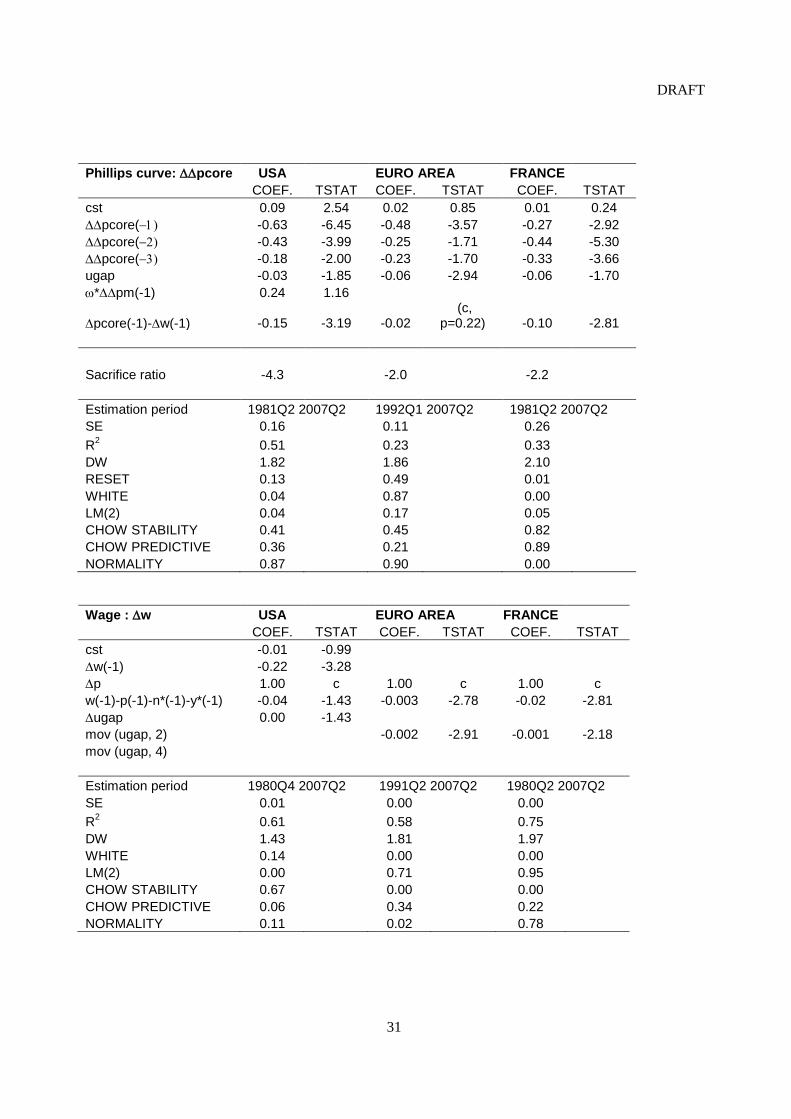
Phillips curve: pcore USA EURO AREA FRANCE


cst 0.09 2.54 0.02 0.85 0.01 0.24

pcore( -0.63 -6.45 -0.48 -3.57 -0.27 -2.92

pcore( -0.43 -3.99 -0.25 -1.71 -0.44 -5.30

pcore( -0.18 -2.00 -0.23 -1.70 -0.33 -3.66

ugap -0.03 -1.85 -0.06 -2.94 -0.06 -1.70

*pm(-1) 0.24 1.16

pcore(-1)-w(-1) -0.15 -3.19 -0.02 (c,

p=0.22) -0.10 -2.81

Sacrifice ratio -4.3

-2.0

-2.2


SE 0.16

0.11

0.26 R

2 0.51

0.23

0.33

DW 1.82

1.86

2.10 RESET 0.13

0.49

0.01

WHITE 0.04

0.87

0.00 LM(2) 0.04

0.17

0.05

CHOW STABILITY 0.41

0.45


0.21

0.89

NORMALITY 0.87 0.90 0.00

Wage : w USA EURO AREA FRANCE


cst -0.01 -0.99

w(-1) -0.22 -3.28 p 1.00 c 1.00 c 1.00 c

w(-1)-p(-1)-n*(-1)-y*(-1) -0.04 -1.43 -0.003 -2.78 -0.02 -2.81

ugap 0.00 -1.43 mov (ugap, 2)

-0.002 -2.91 -0.001 -2.18

mov (ugap, 4)


SE 0.01

0.00

0.00 R

2 0.61

0.58

0.75

DW 1.43

1.81

1.97 WHITE 0.14

0.00

0.00

LM(2) 0.00

0.71

0.95 CHOW STABILITY 0.67

0.00

0.00

CHOW PREDICTIVE 0.06

0.34

0.22 NORMALITY 0.11 0.02 0.78

DRAFT

32

Producer price : p USA EURO AREA FRANCE


cst -0.01 -0.36 0.20 3.39 0.07 1.78

p(-1) 0.50 5.46 p(-2) 0.16 1.55 p(-3) 0.34 (c ) mov(p(-1),8)

0.78 21.17

mov(p(-1),3)

0.61 6.18 mov (gap,4) 0.03 2.26

mov (gap,2)

0.04 2.42

gap(-1)

0.03 1.55


SE 0.22

0.17

0.23 R

2 0.66

0.42

0.83

DW 2.18

2.35

1.58 RESET

0.13

0.13

WHITE 0.00

0.61

0.00 LM(2) 0.00

0.23

0.15

CHOW STABILITY 0.84

0.42


0.82

0.64

NORMALITY 0.75 0.63 0.30

DRAFT

33

ANNEX 3: THE MICRO-FOUNDED DYNAMIC GENERAL EQUILIBRIUM MODEL

This annex details the features of the DGE model used in the paper and provides the micro-foundations of

the different equations. It subsequently describes the calibration of the model for the euro area.

1. Main equations of the DGE model

Keys to variables:

𝐶 Consumption 𝜏𝑤 Tax on labour income

𝐶𝑜 Consumption by intertemporal optimisers 𝜏𝑒 Employer social security contribution

𝜆𝑜 Marginal utility of consumption of

intertemporal optimisers 𝑅 Gross benefit replacement rate

𝐶𝑘 Consumption under liquidity constraints 𝑇 Lump-sum taxes

𝜆𝑘 Marginal utility of consumption of liquidity-

constraint households 𝑌 Output

𝑁 Employment 𝐵 Government bonds bought at the start of

period t

𝑊 Nominal wage 𝑖 Nominal interest rate

𝑃 Price 𝜋 Inflation

𝜏𝑐 Tax on consumption

Consumption: 𝐶𝑡 = 1 − 𝜔 𝐶𝑡𝑜 + 𝜔𝐶𝑡

𝑘

1 = 𝛽 1 + 𝑖𝑡 𝐸𝑡 𝜆𝑡+1𝑜 𝜆𝑡

𝑜

𝜆𝑡𝑜 =

1

1 + 𝜏𝑡𝑐 𝑃𝑡

1

𝐶𝑡𝑜 − ℎ𝐶𝑡−1

𝑜 −𝛽ℎ

𝐶𝑡+1𝑜 − ℎ𝐶𝑡

𝑜

𝐶𝑡𝑘 =

1 − 𝜏𝑡𝑤

1 + 𝜏𝑡𝑐

𝑊𝑡

𝑃𝑡𝑁𝑡 +

1 − 𝜏𝑡𝑤

1 + 𝜏𝑡𝑐 1 − 𝑁𝑡

𝑊𝑡

𝑃𝑡𝑅𝑡 −

𝜛

1 + 𝜏𝑡𝑐

𝑇𝑡

𝑃𝑡

Wages:

𝑊𝑡

𝑃𝑡 1 − 𝜔

1


𝑜 −𝛽ℎ


𝑜 + 𝜔1

𝐶𝑡𝑘 =

1 + 𝜏𝑡𝑐

1 − 𝜏𝑡𝑤

𝜅𝜂𝑁𝑡𝜑

1 − 𝑅𝑡 𝜂 − 1

Production:

𝑌𝑡 = 𝑁𝑡

DRAFT

34

Demand:

𝑌𝑡 = 𝐶𝑡 +𝜙

2

𝑁𝑡

𝑁𝑡−1− 1

2

𝑁𝑡−1 +𝜃

2

𝑃𝑡

𝑃𝑡−1− 1

2

𝑌𝑡

Prices:

𝜃 𝑃𝑡

𝑃𝑡−1− 1

𝑃𝑡

𝑃𝑡−1

= 1 + 𝜃𝐸𝑡 𝛽𝜆𝑡+1𝑜

𝜆𝑡𝑜

𝑃𝑡+1

𝑃𝑡− 1

𝑃𝑡+1

𝑃𝑡

𝑌𝑡+1

𝑌𝑡

+ 𝜀 1 + 𝜏𝑡

𝑒 𝑊𝑡

𝑃𝑡+ 𝜙

𝑌𝑡𝑌𝑡−1

− 1 − 𝛽𝐸𝑡 𝑌𝑡+1

𝑌𝑡− 1

𝑌𝑡+1

𝑌𝑡 +

1

2


− 1 2 𝑃𝑡𝑌𝑡−1

𝑃𝑡−1𝑌𝑡 − 1

Government budget:

1 − 𝜏𝑡𝑤 1 − 𝑁𝑡 𝑊𝑡𝑅𝑡 + 1 + 𝑖𝑡 𝐵𝑡 = 𝜏𝑡

𝑤 + 𝜏𝑡𝑒 𝑊𝑡𝑁𝑡 + 𝜏𝑡

𝑐𝑃𝑡𝐶𝑡 + 𝑇𝑡+𝐵𝑡+1

Monetary policy rule:

𝑖𝑡 = −ln𝛽 + 𝜙𝜋𝜋𝑡

2. Micro-foundations of the equations

The model equations can be derived from assumptions on the behaviour of households, firms and policy

makers.

Households

The household sector consists of a continuum of households 𝑖 ∈ 0,1 . A share 𝜔 of these households faces

liquidity constraints. Liquidity-constrained households, labelled 𝑘 ∈ 0, 𝜔 , have no access to financial

markets and consume their current disposable income at each period. By contrast, unconstraint households,

labelled 𝑜 ∈ 𝜔, 1 , have full access to financial markets. They can buy and sell assets and transfer income

over time.

Lifetime utility is the expected discounted value of utility at each period over an infinite horizon. Utility is

additive in the utility from consumption 𝐶𝑡 and the disutility from work 𝑁𝑡 :

𝐸0 𝛽𝑡(𝑙𝑛 𝐶𝑡𝑖 − ℎ𝐶𝑡−1

𝑖 −𝜅

1 + 𝜑 𝑁𝑡

𝑖 1+𝜑

)

∞

𝑡=0

(1)

DRAFT

35

where 0 ≤ ℎ ≤ 1 indicates the degree of habit persistence, and 𝜅 the weight of leisure . The parameters 𝛽

and 𝜑−1 respectively denote the discount factor and the labour supply elasticity. h is assumed to be zero

for the liquidity-constrained households.

Each household 𝑖 supplies differentiated labour services in a monopolistically competitive labour market.

For simplicity the labour services of liquidity-constrained and intertemporally optimising households are

assumed to be of comparable quality. Labour inputs are then combined in a CES bundle of the

differentiated labour services:

𝑁𝑡 = 𝑁𝑡𝑖

𝜂−1

𝜂 𝑑𝑖1

0

𝜂

𝜂−1

𝜂 is the elasticity of substitution between services. Demand for variety 𝑖 is a function of relative wage and

of total labour demand:

𝑁𝑡𝑖 =

𝑊𝑡𝑖

𝑊𝑡 −𝜂

𝑁𝑡 (2)

The budget constraint of unrestricted households is:

1 − 𝜏𝑡𝑤 𝑊𝑡

𝑖𝑁𝑡𝑜 + 1 − 𝜏𝑡

𝑤 1 − 𝑁𝑡𝑜 𝑊𝑡𝑅𝑡 + 𝑃𝑡𝐷𝑡 = 1 + 𝜏𝑡

𝑐 𝑃𝑡𝐶𝑡𝑜 + 𝐵𝑡+1 − 1 + 𝑖𝑡 𝐵𝑡 + 1 − 𝜛 𝑇𝑡

(3)

with 𝑊𝑡𝑖 the nominal wage of household 𝑖, 𝑊𝑡 the average nominal wage, 𝜏𝑡

𝑤 is the labour income tax, 𝑅𝑡

the replacement ratio for the non-employed part of the household, 𝑃𝑡𝐷𝑡 profits, 𝑃𝑡𝐶𝑡𝑜 nominal

consumption, 𝜏𝑡𝑐 the consumption tax rate 𝐵𝑡are one-period government bonds bought at the start of

period 𝑡, 𝑖𝑡 the nominal interest rate, and 𝑇𝑡 lump-sum taxes. The parameter 1 − 𝜛 is the share of lump-

sum taxes levied from the non liquidity-constrained households.

Liquidity-constrained households can neither save income nor borrow against future income. They do not

receive any profit. As a result, net household expenditure equals net spending at each period:

1 − 𝜏𝑡𝑤 𝑊𝑡

𝑖𝑁𝑡𝑘 + 1 − 𝜏𝑡

𝑤 1 − 𝑁𝑡𝑘 𝑊𝑡𝑅𝑡 = 1 + 𝜏𝑡

𝑐 𝑃𝑡𝐶𝑡𝑘 + 𝜛𝑇𝑡 (4)

Consumption

Households consume a bundle of differentiated goods, each one being provided by a firm 𝑗 ∈ 0,1 . Aggregate consumption thus equals:

𝐶𝑡 = 𝐶𝑡𝑗 𝜀−1𝜀 𝑑𝑗

1

0

𝜀𝜀−1

with 𝜀 as the elasticity of substitution between 𝐶𝑡𝑗. Demand for 𝐶𝑡

𝑗 depends on the relative price of the

variety and on the aggregate demand for consumption goods:

𝑪𝒕𝒋

= 𝑷𝒕

𝒋

𝑷𝒕

−𝜺

𝑪𝒕

(5)

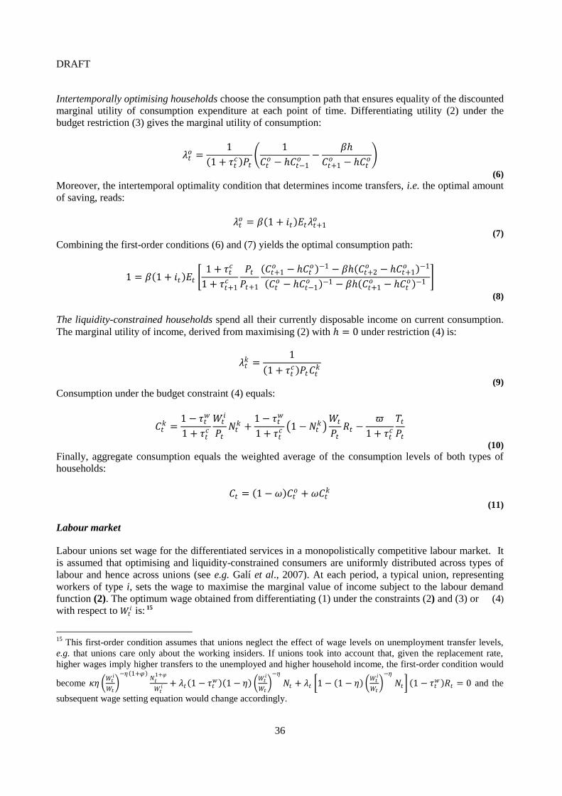
DRAFT

36

Intertemporally optimising households choose the consumption path that ensures equality of the discounted

marginal utility of consumption expenditure at each point of time. Differentiating utility (2) under the

budget restriction (3) gives the marginal utility of consumption:

𝜆𝑡𝑜 =

1

1 + 𝜏𝑡𝑐 𝑃𝑡

1


𝑜 −𝛽ℎ


𝑜

(6)

Moreover, the intertemporal optimality condition that determines income transfers, i.e. the optimal amount

of saving, reads:

𝜆𝑡𝑜 = 𝛽 1 + 𝑖𝑡 𝐸𝑡𝜆𝑡+1

𝑜 (7)

Combining the first-order conditions (6) and (7) yields the optimal consumption path:

1 = 𝛽 1 + 𝑖𝑡 𝐸𝑡 1 + 𝜏𝑡

𝑐

1 + 𝜏𝑡+1𝑐

𝑃𝑡

𝑃𝑡+1


𝑜 −1 − 𝛽ℎ 𝐶𝑡+2𝑜 − ℎ𝐶𝑡+1

𝑜 −1


𝑜 −1 − 𝛽ℎ 𝐶𝑡+1𝑜 − ℎ𝐶𝑡

𝑜 −1

(8)

The liquidity-constrained households spend all their currently disposable income on current consumption.

The marginal utility of income, derived from maximising (2) with ℎ = 0 under restriction (4) is:

𝜆𝑡𝑘 =

1

1 + 𝜏𝑡𝑐 𝑃𝑡𝐶𝑡

𝑘

(9)

Consumption under the budget constraint (4) equals:

𝐶𝑡𝑘 =

1 − 𝜏𝑡𝑤

1 + 𝜏𝑡𝑐

𝑊𝑡𝑖

𝑃𝑡𝑁𝑡

𝑘 +1 − 𝜏𝑡

𝑤

1 + 𝜏𝑡𝑐 1 − 𝑁𝑡

𝑘 𝑊𝑡

𝑃𝑡𝑅𝑡 −

𝜛

1 + 𝜏𝑡𝑐

𝑇𝑡

𝑃𝑡

(10)

Finally, aggregate consumption equals the weighted average of the consumption levels of both types of

households:

𝐶𝑡 = 1 − 𝜔 𝐶𝑡𝑜 + 𝜔𝐶𝑡

𝑘 (11)

Labour market

Labour unions set wage for the differentiated services in a monopolistically competitive labour market. It

is assumed that optimising and liquidity-constrained consumers are uniformly distributed across types of

labour and hence across unions (see e.g. Galí et al., 2007). At each period, a typical union, representing

workers of type i, sets the wage to maximise the marginal value of income subject to the labour demand

function (2). The optimum wage obtained from differentiating (1) under the constraints (2) and (3) or (4)

with respect to 𝑊𝑡𝑖 is: 15

15

This first-order condition assumes that unions neglect the effect of wage levels on unemployment transfer levels,

e.g. that unions care only about the working insiders. If unions took into account that, given the replacement rate,

higher wages imply higher transfers to the unemployed and higher household income, the first-order condition would

become 𝜅𝜂 𝑊𝑡

𝑖

𝑊𝑡 −𝜂 1+𝜑

𝑁𝑡1+𝜑

𝑊𝑡𝑖 + 𝜆𝑡 1 − 𝜏𝑡

𝑤 1 − 𝜂 𝑊𝑡

𝑖

𝑊𝑡 −𝜂

𝑁𝑡 + 𝜆𝑡 1 − 1 − 𝜂 𝑊𝑡

𝑖

𝑊𝑡 −𝜂

𝑁𝑡 1 − 𝜏𝑡𝑤 𝑅𝑡 = 0 and the

subsequent wage setting equation would change accordingly.

DRAFT

37

𝜅𝜂 𝑊𝑡

𝑖

𝑊𝑡

−𝜂 1+𝜑 𝑁𝑡

1+𝜑

𝑊𝑡𝑖

+ 𝜆𝑡 1 − 𝜏𝑡𝑤 1 − 𝜂

𝑊𝑡𝑖

𝑊𝑡

−𝜂

𝑁𝑡 + 𝜆𝑡𝜂 1 − 𝜏𝑡𝑤

𝑊𝑡𝑖

𝑊𝑡

− 1+𝜂

𝑁𝑡𝑅𝑡 = 0

All unions target the same wage and wages are fully flexible, so that 𝑊𝑡𝑖 = 𝑊𝑡 , the previous expression

simplifies to:

𝑊𝑡 =𝜅

1 − 𝜏𝑡𝑤

𝑁𝑡𝜑

𝜆𝑡

𝜂

1 − 𝑅𝑡 𝜂 − 1

The replacement rate, a proxy of the reservation wage, exerts upward pressures on wages. Because

consumption generally differs across both types of households, the union weights labour income using a

weighted average of constrained and unconstrained households’ marginal utility of consumption, i.e.

𝜆𝑡 = 1 − 𝜔 𝜆𝑡𝑜 + 𝜔𝜆𝑡

𝑘 . Inserting (6) along this weighting scheme yields:

𝑊𝑡

𝑃𝑡 1 − 𝜔

1


𝑜 −𝛽ℎ


𝑜 + 𝜔1

𝐶𝑡𝑘 =

1 + 𝜏𝑡𝑐

1 − 𝜏𝑡𝑤

𝜅𝜂𝑁𝑡𝜑

1 − 𝑅𝑡 𝜂 − 1

(12)

Because firms allocate labour demand uniformly across different workers employment is equal across

households, i.e. 𝑁𝑡 = 𝑁𝑡𝑜 = 𝑁𝑡

𝑘 .

Production and prices

The production sector consists of a continuum of firms 𝑗 ∈ 0,1 producing a differentiated product and

setting price in a monopolistically competitive goods market. Labour is the only input, which yields

constant returns to scale. Without loss of generality, the technology parameter can be normalised to one.

Consequently, gross output of firm 𝑗 under this simple production function is:

𝑌𝑡𝑗

= 𝑁𝑡𝑗

(13)

Each firm faces quadratic employment and price adjustment costs Φt and Θt respectively. Adjustment

costs are sunk costs that use part of output and drive a wedge between production and consumption.

Labour adjustment costs can be interpreted as hiring and firing costs. A common specification of quadratic

per-unit adjustment costs of firm 𝑗 (see e.g. Cahuc and Zylberberg, 2004; Hamermesh, 1995; Rotemberg,

1982) is:

Φ𝑡𝑗

=𝜙

2

𝑁𝑡𝑗

𝑁𝑡−1𝑗

− 1

2

Θ𝑡𝑗

=𝜃

2

𝑃𝑡𝑗

𝑃𝑡−1𝑗

− 1

2

The aggregate level of output is:

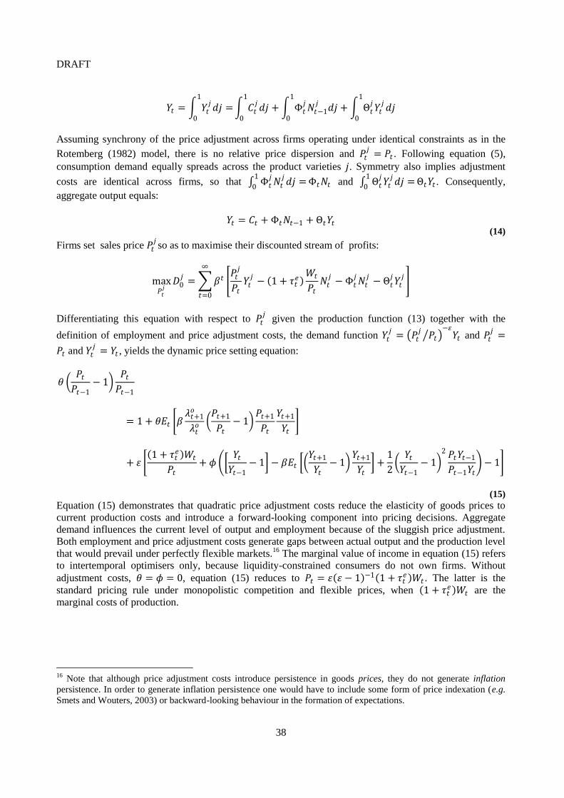
DRAFT

38

𝑌𝑡 = 𝑌𝑡𝑗𝑑𝑗 =

1

0

𝐶𝑡𝑗𝑑𝑗

1

0

+ Φ𝑡𝑗𝑁𝑡−1

𝑗𝑑𝑗

1

0

+ Θ𝑡𝑗𝑌𝑡

𝑗𝑑𝑗

1

0

Assuming synchrony of the price adjustment across firms operating under identical constraints as in the

Rotemberg (1982) model, there is no relative price dispersion and 𝑃𝑡𝑗

= 𝑃𝑡 . Following equation (5),

consumption demand equally spreads across the product varieties 𝑗. Symmetry also implies adjustment

costs are identical across firms, so that Φ𝑡𝑗𝑁𝑡

𝑗𝑑𝑗 =

1

0Φ𝑡𝑁𝑡 and Θ𝑡

𝑗𝑌𝑡

𝑗𝑑𝑗 =

1

0Θ𝑡𝑌𝑡 . Consequently,

aggregate output equals:

𝑌𝑡 = 𝐶𝑡 + Φ𝑡𝑁𝑡−1 + Θ𝑡𝑌𝑡 (14)

Firms set sales price 𝑃𝑡𝑗so as to maximise their discounted stream of profits:

max𝑃𝑡

𝑗𝐷0

𝑗= 𝛽𝑡

∞

𝑡=0

𝑃𝑡

𝑗

𝑃𝑡𝑌𝑡

𝑗− 1 + 𝜏𝑡

𝑒 𝑊𝑡

𝑃𝑡𝑁𝑡

𝑗− Φ𝑡

𝑗𝑁𝑡

𝑗− Θ𝑡

𝑗𝑌𝑡

𝑗

Differentiating this equation with respect to 𝑃𝑡𝑗 given the production function (13) together with the

definition of employment and price adjustment costs, the demand function 𝑌𝑡𝑗

= 𝑃𝑡𝑗

𝑃𝑡 −𝜀

𝑌𝑡 and 𝑃𝑡𝑗

=

𝑃𝑡 and 𝑌𝑡𝑗

= 𝑌𝑡 , yields the dynamic price setting equation:

𝜃 𝑃𝑡

𝑃𝑡−1− 1

𝑃𝑡

𝑃𝑡−1


𝜆𝑡𝑜

𝑃𝑡+1

𝑃𝑡− 1

𝑃𝑡+1

𝑃𝑡

𝑌𝑡+1

𝑌𝑡

+ 𝜀 1 + 𝜏𝑡

𝑒 𝑊𝑡

𝑃𝑡+ 𝜙


− 1 − 𝛽𝐸𝑡 𝑌𝑡+1

𝑌𝑡− 1

𝑌𝑡+1

𝑌𝑡 +

1

2


− 1 2 𝑃𝑡𝑌𝑡−1

𝑃𝑡−1𝑌𝑡 − 1

(15)

Equation (15) demonstrates that quadratic price adjustment costs reduce the elasticity of goods prices to

current production costs and introduce a forward-looking component into pricing decisions. Aggregate

demand influences the current level of output and employment because of the sluggish price adjustment.

Both employment and price adjustment costs generate gaps between actual output and the production level

that would prevail under perfectly flexible markets.16

The marginal value of income in equation (15) refers

to intertemporal optimisers only, because liquidity-constrained consumers do not own firms. Without

adjustment costs, 𝜃 = 𝜙 = 0, equation (15) reduces to 𝑃𝑡 = 𝜀 𝜀 − 1 −1 1 + 𝜏𝑡𝑒 𝑊𝑡 . The latter is the

standard pricing rule under monopolistic competition and flexible prices, when 1 + 𝜏𝑡𝑒 𝑊𝑡 are the

marginal costs of production.

16

Note that although price adjustment costs introduce persistence in goods prices, they do not generate inflation

persistence. In order to generate inflation persistence one would have to include some form of price indexation (e.g.

Smets and Wouters, 2003) or backward-looking behaviour in the formation of expectations.

DRAFT

39

Government

The Government collects wage income tax 𝜏𝑡𝑤 , consumption tax 𝜏𝑡

𝑐 , and employer social security

contributions 𝜏𝑡𝑒 . It pays transfers at the replacement rate 𝑅𝑡 to unemployed household members and issues

bonds 𝐵𝑡+1 to balance the budget. It can also levy lump-sum taxes 𝑇𝑡 to this aim. Public final demand is

omitted for simplicity, but this would not substantially modify the results. The government budget

constraint is:

1 − 𝜏𝑡𝑤 1 − 𝑁𝑡 𝑊𝑡𝑅𝑡 + 1 + 𝑖𝑡 𝐵𝑡 = 𝜏𝑡

𝑤 + 𝜏𝑡𝑒 𝑊𝑡𝑁𝑡 + 𝜏𝑡

𝑐𝑃𝑡𝐶𝑡 + 𝑇𝑡+𝐵𝑡+1 (16)

Forward-looking consumption and price setting behaviour requires a policy rule to ensure the uniqueness

and stability of the equilibrium. To keep the analysis simple, policy rates are assumed to react to current

inflation:

𝑖𝑡 = −ln𝛽 + 𝜙𝜋𝜋𝑡 (17)

Extension: A search and matching model of the labour market

A number of recent contributions have adopted the search-and-matching approach in DGE models to

incorporate the effect of frictional unemployment in the analysis (e.g. Blanchard and Galí, 2008;

Campolmi and Faia, 2006; Christoffel and Linzert, 2005; Faia, 2006).

Frictional unemployment allows gross to differ from net flows into and out of unemployment. The

framework in the present paper uses the wage setting relationship (12). The derivation explicitly accounts

for the impact of structural policies on steady-state labour supply instead of adopting the common

assumption of exogenous and constant labour supply. For simplicity we restrict this model extension to an

economy without liquidity-constrained consumers, i.e. to 𝜔 = 0.

Employment 𝑁𝑡 is modelled as the level of previous employment net of job separations plus current job

matches:

𝑁𝑡 = 1 − 𝜌 𝑁𝑡−1 + 𝑚 𝑈𝑡 , 𝑉𝑡 (18)

where 𝜌 is an exogenous separation rate, and 𝑚 𝑈𝑡 ,𝑉𝑡 are current job matches given initial unemployment

𝑈𝑡 and vacancies 𝑉𝑡 . The matching function has a Cobb-Douglass form (e.g. Campolmi and Faia, 2006;

Faia, 2006):

𝑚 𝑈𝑡 , 𝑉𝑡 = 𝜇𝑈𝑡𝜉𝑉𝑡

1−𝜉

with 𝜇 ∈ 0,1 as the matching technology and 𝜉 ∈ 0,1 specifying the elasticity of matches with respect

to unemployment. Unemployment at the start of the period 𝑈𝑡 , is the gap between labour supply, i.e.

optimal employment, in the absence of employment and price adjustment costs 𝐿𝑡𝑠 , and actual beginning-

of-period employment: 𝑈𝑡 = 𝐿𝑡𝑠 − 1 − 𝜌 𝑁𝑡−1.

17 The ratio of vacancies over unemployment 𝜗𝑡 = 𝑉𝑡 𝑈𝑡 ,

is a measure of labour market tightness that allows rewriting the matching function:

17

This contrasts with the previously cited research. The latter generally defines unemployment as the gap between a

constant work force, often normalised to unity, and actual employment. The definition adopted here accounts for the

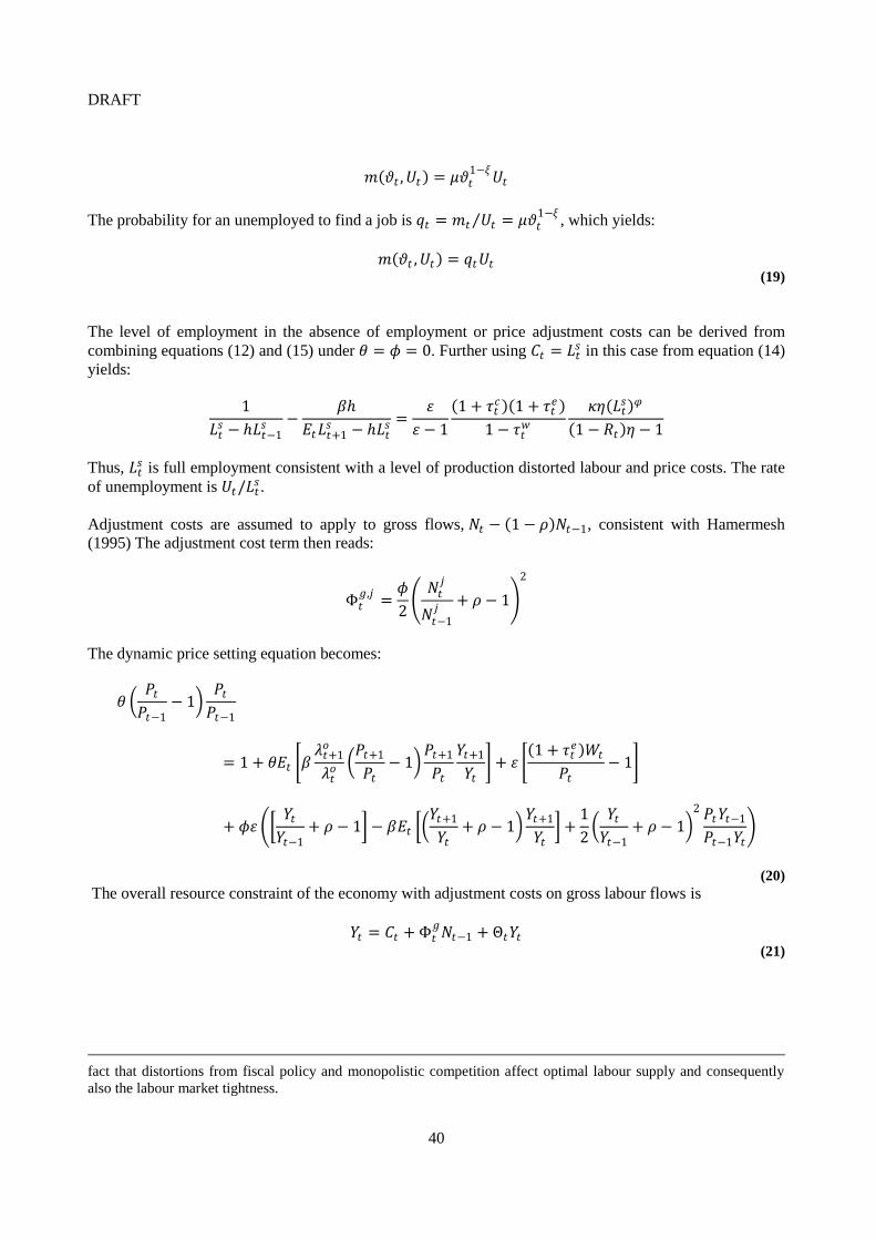
DRAFT

40

𝑚 𝜗𝑡 ,𝑈𝑡 = 𝜇𝜗𝑡1−𝜉

𝑈𝑡

The probability for an unemployed to find a job is 𝑞𝑡 = 𝑚𝑡 𝑈𝑡 = 𝜇𝜗𝑡1−𝜉

, which yields:

𝑚 𝜗𝑡 ,𝑈𝑡 = 𝑞𝑡𝑈𝑡 (19)

The level of employment in the absence of employment or price adjustment costs can be derived from

combining equations (12) and (15) under 𝜃 = 𝜙 = 0. Further using 𝐶𝑡 = 𝐿𝑡𝑠 in this case from equation (14)

yields:

1

𝐿𝑡𝑠 − ℎ𝐿𝑡−1

𝑠 −𝛽ℎ

𝐸𝑡𝐿𝑡+1𝑠 − ℎ𝐿𝑡

𝑠 =𝜀

𝜀 − 1

1 + 𝜏𝑡𝑐 1 + 𝜏𝑡

𝑒

1 − 𝜏𝑡𝑤

𝜅𝜂 𝐿𝑡𝑠 𝜑

1 − 𝑅𝑡 𝜂 − 1

Thus, 𝐿𝑡𝑠 is full employment consistent with a level of production distorted labour and price costs. The rate

of unemployment is 𝑈𝑡/𝐿𝑡𝑠.

Adjustment costs are assumed to apply to gross flows, 𝑁𝑡 − 1 − 𝜌 𝑁𝑡−1, consistent with Hamermesh

(1995) The adjustment cost term then reads:

Φ𝑡𝑔,𝑗

=𝜙

2

𝑁𝑡𝑗

𝑁𝑡−1𝑗

+ 𝜌 − 1

2

The dynamic price setting equation becomes:

𝜃 𝑃𝑡

𝑃𝑡−1− 1

𝑃𝑡

𝑃𝑡−1


𝜆𝑡𝑜

𝑃𝑡+1

𝑃𝑡− 1

𝑃𝑡+1

𝑃𝑡

𝑌𝑡+1

𝑌𝑡 + 𝜀

1 + 𝜏𝑡𝑒 𝑊𝑡

𝑃𝑡− 1

+ 𝜙𝜀 𝑌𝑡

𝑌𝑡−1+ 𝜌 − 1 − 𝛽𝐸𝑡

𝑌𝑡+1

𝑌𝑡+ 𝜌 − 1

𝑌𝑡+1

𝑌𝑡 +

1

2


+ 𝜌 − 1 2 𝑃𝑡𝑌𝑡−1

𝑃𝑡−1𝑌𝑡

(20)

The overall resource constraint of the economy with adjustment costs on gross labour flows is

𝑌𝑡 = 𝐶𝑡 + Φ𝑡𝑔𝑁𝑡−1 + Θ𝑡𝑌𝑡

(21)

fact that distortions from fiscal policy and monopolistic competition affect optimal labour supply and consequently

also the labour market tightness.

DRAFT

41

3. Calibration

The calibration of the model parameters builds on the estimated euro area DGE models of Coenen et al.

(2007) and Grenouilleau et al. (2007), mark-up estimates of Christopoulou and Vermeulen (2008) and tax

and benefit data from OECD (2007) (see Table A.3.1).

The parameter of price adjustment costs matches the empirical evidence on average price duration in the

euro area and the United States (Bils and Klenow, 2004; Altissimo et al., 2006). The value of 25% for the

share of liquidity-constrained households in Figures 7-8 and A.4.5-A.4.8 is taken from Coenen et al.

(2007). The fiscal parameters follow the OECD (2007) tax and benefits data for euro area countries and

coincide with those in Coenen et al. (2007). The average replacement rate is the one for spouse in work,

because unemployment in the model is for second earner in the model. The estimated average elasticity of

substitution in the goods market in Christopoulou and Vermeulen (2008) suggests a 25% price mark-up.

Following Coenen et al. (2007) for the elasticity of substitution between labour services, the steady-state

wage mark-up is 20%. The remaining parameter values are taken from the euro area models of Coenen et

al. (2007) and Smets and Wouters (2003) and are in line with other empirical studies.

Table A.3.1: Calibration of the parameters

Name Symbol Value Source

Employment adjustment costs

Euro area

United States

θ

63

30

Grenouilleau et al. (2007)

Price adjustment costs

Euro area

United States

ψ

21

3.40

Grenouilleau et al. (2007)

Consumption tax τc 0.18 OECD (2007)

Labour income tax τw 0.24 OECD (2007)

Employer social security contributions τe 0.22 OECD (2007)

Replacement rate R 0.25 OECD (2007)

Elasticity of substitution between types of labour η 6.00 Coenen et al. (2007)

Elasticity of substitution between types of goods ε 5.00 Christopoulou and Vermeulen (2008)

Habit persistence h 0.85 Grenouilleau et al. (2007)

Share of liquidity-constrained households ω 0.25 Coenen et al. (2007)

Disutility weight of labour κ 1.00 Coenen et al. (2007)

Discount factor β 0.99 Coenen et al. (2007)

Inverse of labour supply elasticity φ 2.20 Smets and Wouters (2003)

Policy response to inflation 𝜙𝜋 1.50 Galí et al. (2007)

Job finding probability 𝑞 0.60 Campolmi and Faia (2007)

Exogenous job separation rate ρ 0.08 Christoffel and Linzert (2005)

REFERENCES

Altissimo, F., M. Ehrmann and F. Smets (2006), “Inflation Persistence and Price-Setting Behaviour in

the Euro Area: A Summary of the IPN Evidence”, ECB Occasional Papers, No. 46.

DRAFT

42

Bils, M. and P. Klenow (2004), “Some Evidence on the Importance of Sticky Prices”, Journal of

Political Economy, Vol. 112, No. 5, pp. 947-984.

Blanchard, O. and J. Galí (2008), “Labour Markets and Monetary Policy: A New-Keynesian Model

with Unemployment”, NBER Working Paper, No. 13897.

Cahuc, P. and A. Zylberberg (2004), Labour Economics, MIT Press, Cambridge, Mass.

Campolmi, A. and E. Faia (2006), “Cyclical Inflation Divergence and Different Labor Market

Institutions in the EMU”, ECB Working Papers, No. 619.

Christoffel, K. and T. Linzert (2005), “The Role of Real Wage Dynamics and Labor Market Frictions

for Unemployment and Inflation Dynamics”, ECB Working Papers, No. 556.

Christopoulou, R. and Ph. Vermeulen (2008), “Markups in the Euro Area and the US over the Period

1981-2004”, ECB Working Papers, No. 856.

Coenen, G., P. McAdam and R. Straub (2007), “Tax Reform and Labour-Market Performance in the

Euro Area: A Simulation-Based Analysis Using the New Area-Wide Model”, ECB Working Papers, No.

747.

Faia, E. (2006), “Optimal Monetary Policy Rules with Labor Market Frictions”, ECB Working

Papers, No. 698.

Galí, J., D. López-Salido and J. Vallés (2007), “Understanding the Effects of Government Spending

on Consumption”, Journal of the European Economic Association, Vol. 5, No. 1, pp. 227-270.

Grenouilleau, D., M. Ratto and W. Roeger (2007), “Adjustment to Shocks: A Comparison between

the Euro Area and the US Using Estimated DSGE Models”, paper presented at the Workshop on Structural

Reforms and Economic Resilience, OECD, Paris, 14 June.

Hamermesh, D. (1995), “Labour Demand and the Source of Adjustment Costs”, Economic Journal,

Vol. 105, No. 430, pp. 620-634.

OECD (2007), Benefits and Wages, OECD, Paris.

Rotemberg, J. (1982), “Monopolistic Price Adjustment and Aggregate Output”, Review of Economic

Studies, Vol. 49, No. 4, pp. 517-31.

Smets, F. and R. Wouters (2003), “An Estimated Dynamic Stochastic General Equilibrium Model of

the Euro Area”, Journal of the European Economic Association, Vol. 1, No. 5, pp. 1123-1175.

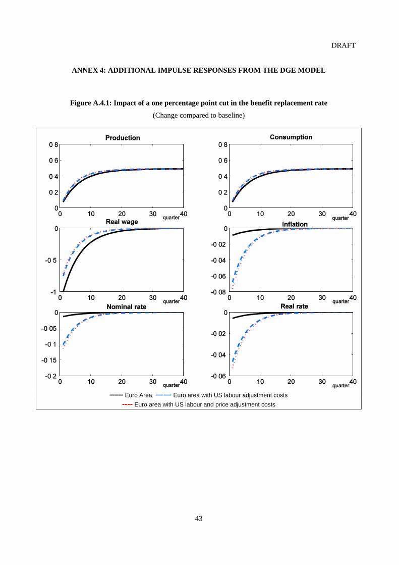
DRAFT

43

ANNEX 4: ADDITIONAL IMPULSE RESPONSES FROM THE DGE MODEL

Figure A.4.1: Impact of a one percentage point cut in the benefit replacement rate


––– Euro Area ―― Euro area with US labour adjustment costs


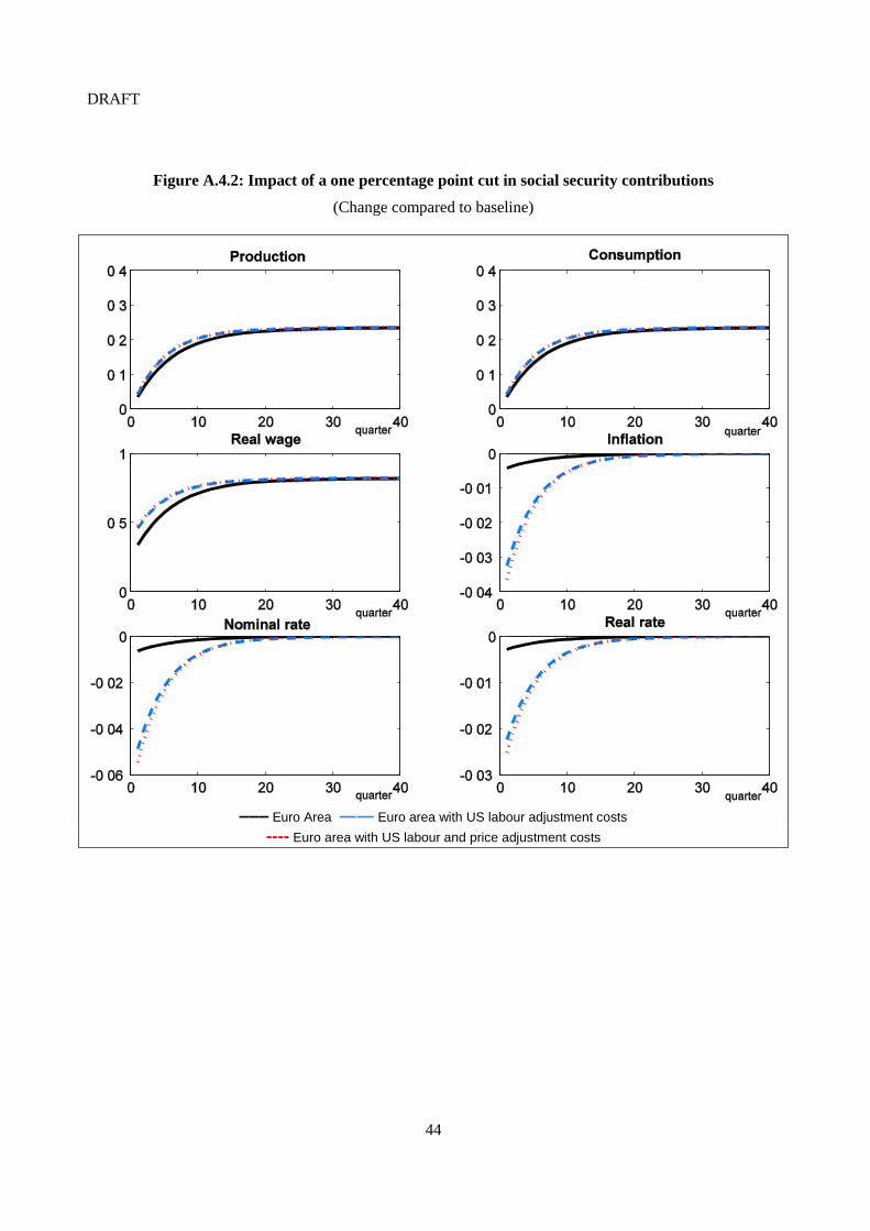
DRAFT

44

Figure A.4.2: Impact of a one percentage point cut in social security contributions




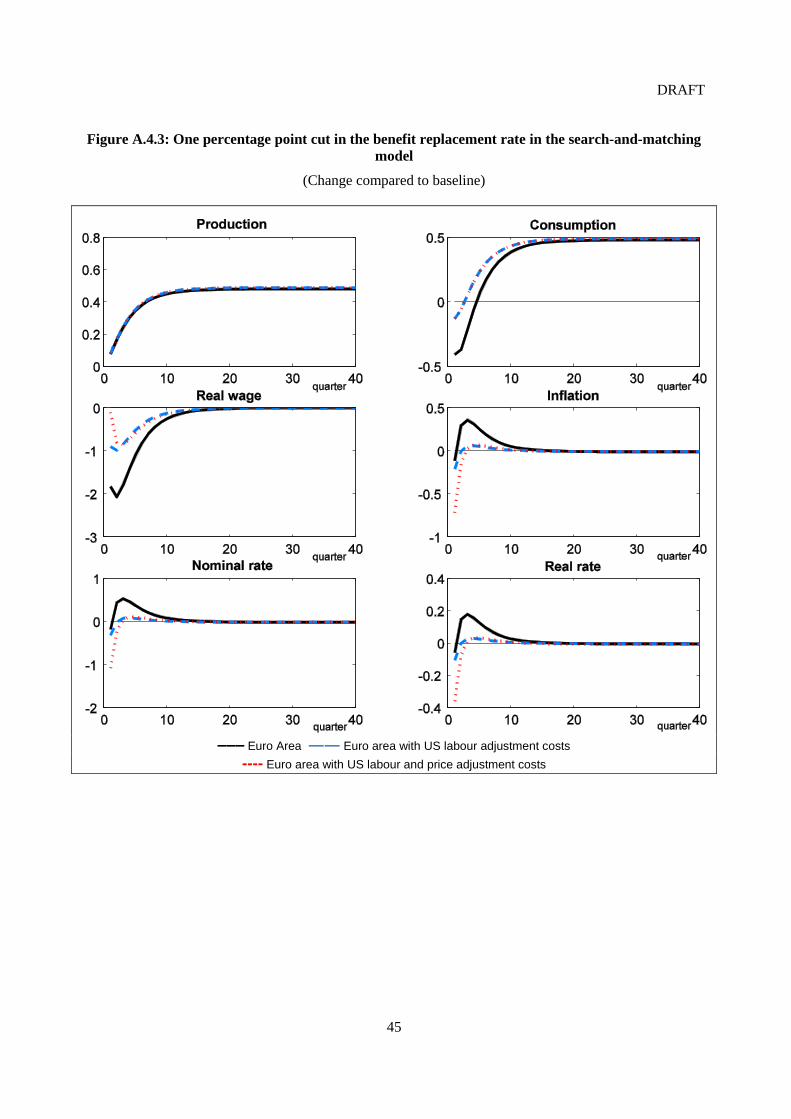
DRAFT

45

Figure A.4.3: One percentage point cut in the benefit replacement rate in the search-and-matching

model




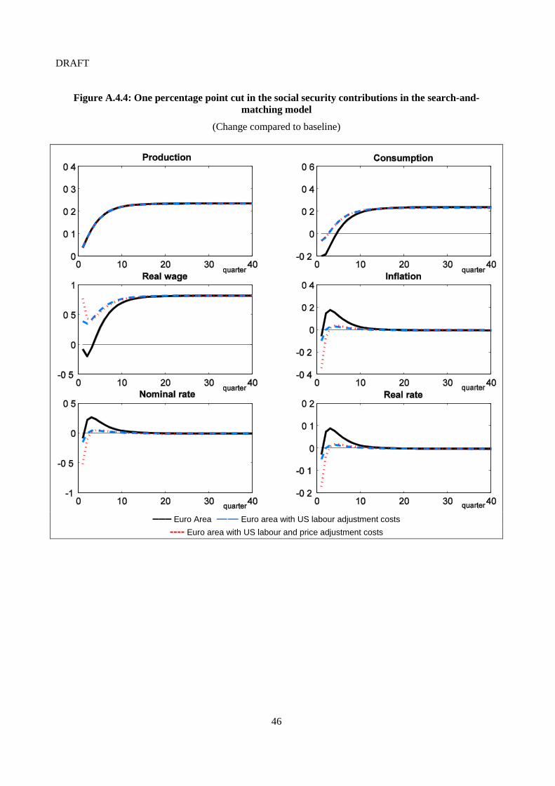
DRAFT

46

Figure A.4.4: One percentage point cut in the social security contributions in the search-and-

matching model




DRAFT

47

Figure A.4.5: One percentage point cut in social security contributions in the model with liquidity-

constrained households



US labour and price adjustment costs

DRAFT

48

Figure A.4.6: One percentage point cut in the benefit replacement rate in the model with liquidity-

constrained households under alternative budget-balancing schemes


––– Fiscal surplus to both types of households ―― Fiscal surplus only to optimising households

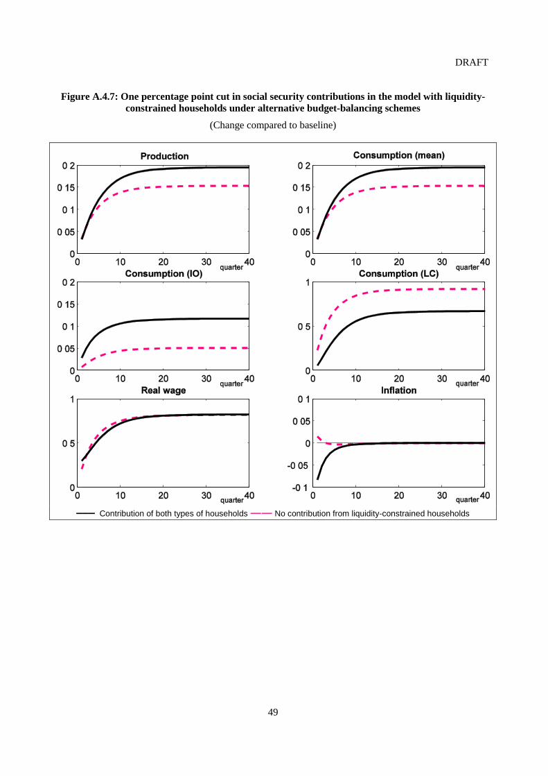
DRAFT

49

Figure A.4.7: One percentage point cut in social security contributions in the model with liquidity-

constrained households under alternative budget-balancing schemes


––– Contribution of both types of households ―― No contribution from liquidity-constrained households

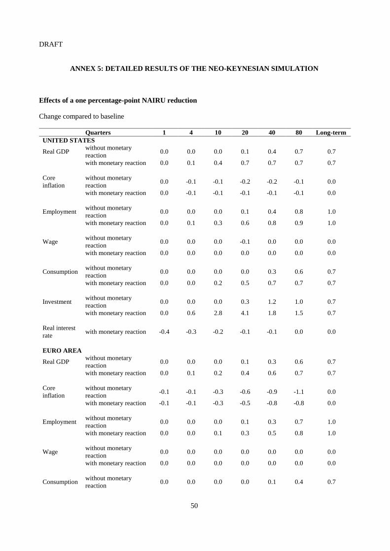
DRAFT

50

ANNEX 5: DETAILED RESULTS OF THE NEO-KEYNESIAN SIMULATION

Effects of a one percentage-point NAIRU reduction

Change compared to baseline

Quarters 1 4 10 20 40 80 Long-term

UNITED STATES

Real GDP without monetary

reaction 0.0 0.0 0.0 0.1 0.4 0.7 0.7

with monetary reaction 0.0 0.1 0.4 0.7 0.7 0.7 0.7

Core

inflation

without monetary

reaction 0.0 -0.1 -0.1 -0.2 -0.2 -0.1 0.0

with monetary reaction 0.0 -0.1 -0.1 -0.1 -0.1 -0.1 0.0

Employment without monetary

reaction 0.0 0.0 0.0 0.1 0.4 0.8 1.0


Wage without monetary

reaction 0.0 0.0 0.0 -0.1 0.0 0.0 0.0


Consumption without monetary

reaction 0.0 0.0 0.0 0.0 0.3 0.6 0.7


Investment without monetary

reaction 0.0 0.0 0.0 0.3 1.2 1.0 0.7


Real interest

rate with monetary reaction -0.4 -0.3 -0.2 -0.1 -0.1 0.0 0.0

EURO AREA


reaction 0.0 0.0 0.0 0.1 0.3 0.6 0.7


Core

inflation

without monetary

reaction -0.1 -0.1 -0.3 -0.6 -0.9 -1.1 0.0

with monetary reaction -0.1 -0.1 -0.3 -0.5 -0.8 -0.8 0.0


reaction 0.0 0.0 0.0 0.1 0.3 0.7 1.0



reaction 0.0 0.0 0.0 0.0 0.0 0.0 0.0



reaction 0.0 0.0 0.0 0.0 0.1 0.4 0.7

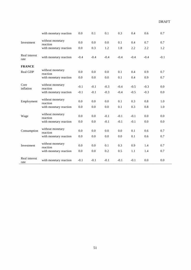
DRAFT

51



reaction 0.0 0.0 0.0 0.1 0.4 0.7 0.7


Real interest

rate with monetary reaction -0.4 -0.4 -0.4 -0.4 -0.4 -0.4 -0.1

FRANCE


reaction 0.0 0.0 0.0 0.1 0.4 0.9 0.7


Core

inflation

without monetary

reaction -0.1 -0.1 -0.3 -0.4 -0.5 -0.3 0.0

with monetary reaction -0.1 -0.1 -0.3 -0.4 -0.5 -0.3 0.0


reaction 0.0 0.0 0.0 0.1 0.3 0.8 1.0



reaction 0.0 0.0 -0.1 -0.1 -0.1 0.0 0.0

with monetary reaction 0.0 0.0 -0.1 -0.1 -0.1 0.0 0.0


reaction 0.0 0.0 0.0 0.0 0.1 0.6 0.7



reaction 0.0 0.0 0.1 0.3 0.9 1.4 0.7


Real interest

rate with monetary reaction -0.1 -0.1 -0.1 -0.1 -0.1 0.0 0.0

the fourteenth dubrovnik economic conference

Documents