THE GEOMETRY OF QUADRATICPOLYNOMIAL DIFFERENTIAL SYSTEMS

WITH A FINITE AND AN INFINITE

SADDLE–NODE (A,B)

JOAN C. ARTESDepartament de Matematiques, Universitat Autonoma de Barcelona,

08193 Bellaterra, Barcelona, SpainE–mail: artes@mat.uab.cat

ALEX C. REZENDE1 AND REGILENE D. S. OLIVEIRA2

Departamento de Matematica, Universidade de Sao Paulo,13566–590, Sao Carlos, Sao Paulo, Brazil,

E–mail: 1arezende@icmc.usp.br, 2regilene@icmc.usp.br

Planar quadratic differential systems occur in many areas of applied mathematics. Althoughmore than one thousand papers have been written on these systems, a complete understandingof this family is still missing. Classical problems, and in particular, Hilbert’s 16th problem[Hilbert, 1900, Hilbert, 1902], are still open for this family. Our aim is to make a global studyof the family QsnSN which is the closure within real quadratic differential systems of the familyQsnSN of all such systems which have two semi–elemental saddle–nodes, one finite and oneinfinite formed by the collision of two infinite singular points. This family can be divided intothree different subfamilies, all of them with the finite saddle–node at the origin of the planewith the eigenvectors on the axes and (A) with the infinite saddle–node in the horizontal axis,(B) with the infinite saddle–node in the vertical axis and (C) with the infinite saddle–node inthe bisector of the first and third quadrants. These three subfamilies modulo the action of theaffine group and time homotheties are three–dimensional (the closure is four–dimensional) andwe give their bifurcation diagram with respect to a normal form. In this paper we provide thecomplete study of the geometry of the first two families, (A) and (B). The bifurcation diagramfor the subfamily (A) yields 38 phase portraits for systems in QsnSN(A) (29 in QsnSN(A))out of which only 3 have limit cycles and 13 possess graphics. The bifurcation diagram for thesubfamily (B) yields 25 phase portraits for systems in QsnSN(B) (16 in QsnSN(B)) out ofwhich 11 possess graphics. None of the 25 portraits has limit cycles. Case (C) will yield manymore phase portraits and will be written separately in a forthcoming new paper. Algebraicinvariants are used to construct the bifurcation set. The phase portraits are represented on thePoincare disk. The bifurcation set of QsnSN(A) is formed by algebraic surfaces and one surfacewhose presence was detected numerically. All points in this surface correspond to connectionsof separatrices. The bifurcation set of QsnSN(B) is formed only by algebraic surfaces.

1

This is a preprint of: “The geometry of quadratic polynomial differential systems with a finite andan infinite saddle-node (A,B)”, Joan Carles Artes, Alex Carlucci Rezende, Regilene D. S. Oliveira,Internat. J. Bifur. Chaos Appl. Sci. Engrg., vol. 24(4), 1450044 (30 pages), 2014.DOI: [10.1142/S0218127414500448]

1. Introduction, brief review of the litera-ture and statement of results

Here we call quadratic differential systems or simplyquadratic systems, differential systems of the form

x = p(x, y),y = q(x, y),

(1)

where p and q are polynomials over R in x and ysuch that the max(deg(p),deg(q)) = 2. To sucha system one can always associate the quadraticvector field

X = p∂

∂x+ q

∂

∂y, (2)

as well as the differential equation

qdx− pdy = 0. (3)

The class of all quadratic differential systems (orquadratic vector fields) will be denoted by QS.

We can also write system (1) as

x = p0 + p1(x, y) + p2(x, y) = p(x, y),y = q0 + q1(x, y) + q2(x, y) = q(x, y),

(4)

where pi and qi are homogeneous polynomials ofdegree i in (x, y) with real coefficients with p22+q22 6=0.

Even after hundreds of studies on the topologyof real planar quadratic vector fields, it is kind ofimpossible to outline a complete characterization oftheir phase portraits, and attempting to topologi-cally classify them is a quite complex task. Thisfamily of systems depends on twelve parameters,but due to the action of the group G of real affinetransformations and time homotheties, the class ul-timately depends on five parameters, but this is stilla large number.

This paper is aimed at studying the classQsnSN which is the closure within real quadraticreal differential systems of the family QsnSN ofall such systems which possess a finite saddle–node sn(2) and an infinite saddle–node of type(02

)SN obtained by the collision of an infinite sad-

dle with an infinite node. The finite saddle–nodeis a semi–elemental point whose neighborhood isformed by the union of two hyperbolic sectors andone parabolic sector. By a semi–elemental pointwe understand a point with zero determinant ofits Jacobian, but only one eigenvalue zero. These

points are known in classical literature as semi–elementary, but we use the term semi–elementalintroduced in [Artes et al., 2012] as part of a set ofnew definitions more deeply related to the geometryof the singular points, their multiplicities and, es-pecially, their Jacobian matrices. We observe thatthere is another type of infinite saddle–node de-

noted by(11

)SN which is given by the collision of

a finite antisaddle (respectively, finite saddle) withan infinite saddle (respectively, infinite node) andwhich will appear in some of the phase portraits.

The condition of having a finite saddle–node ofall the systems in QsnSN implies that these sys-tems may have up to two other finite points.

For a general framework of the study of theclass of all quadratic differential systems we re-fer to the article of Roussarie and Schlomiuk[Roussarie & Schlomiuk, 2002].

In this study we follow the pattern set out in[Artes et al., 2006]. As much as possible we shalltry to avoid repeating technical sections which arethe same for both papers, referring to the papermentioned just above, for more complete informa-tion.

This family can be divided into three differentsubfamilies, all of them with the finite saddle–nodeat the origin of the plane with the eigenvectors onthe axes and (A) with the infinite saddle–node inthe horizontal axis, (B) with the infinite saddle–node in the vertical axis and (C) with the infinitesaddle–node in the bisector of the first and thirdquadrants.

In this article we give a partition of theclasses QsnSN(A) and QsnSN(B). The first classQsnSN(A) is partitioned into 85 parts: 23 three–dimensional ones, 37 two–dimensional ones, 20 one–dimensional ones and 5 points. This partition isobtained by considering all the bifurcation surfacesof singularities, one related to the presence of an-other invariant straight rather than the one statedin statement (a) of Theorem 1.1 and one related toconnections of separatrices, modulo “islands” (seeSec. 8). The second class QsnSN(B) is partitionedinto 43 parts: 9 three–dimensional ones, 18 two–dimensional ones, 12 one–dimensional ones and 4points, which are all delimited by algebraic bifurca-tion surfaces.

A graphic as defined in [Dumortier et al., 1994]is formed by a finite sequence of singular points

2

The geometry of quadratic polynomial differential systems with a finite and an infinite saddle–node (A,B) 3

r1, r2, . . . , rn (with possible repetitions) and non–trivial connecting orbits γi for i = 1, . . . , n suchthat γi has ri as α–limit set and ri+1 as ω–limitset for i < n and γn has rn as α–limit set and r1 asω–limit set. Also normal orientations nj of the non–trivial orbits must be coherent in the sense that ifγj−1 has left–hand orientation then so does γj. Apolycycle is a graphic which has a Poincare returnmap.

A degenerate graphic is a graphic where it isalso allowed that one or several (even all) con-necting orbits γi can be formed by an infinitenumber of singular points. For more details, see[Dumortier et al., 1994].

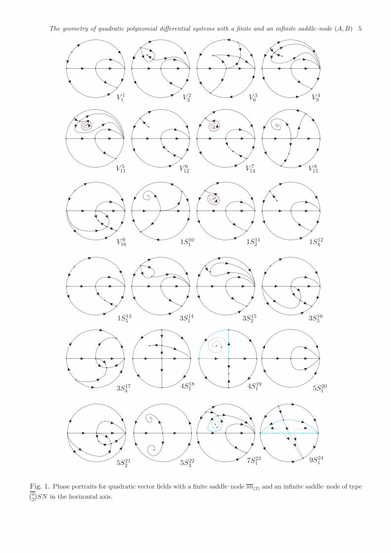
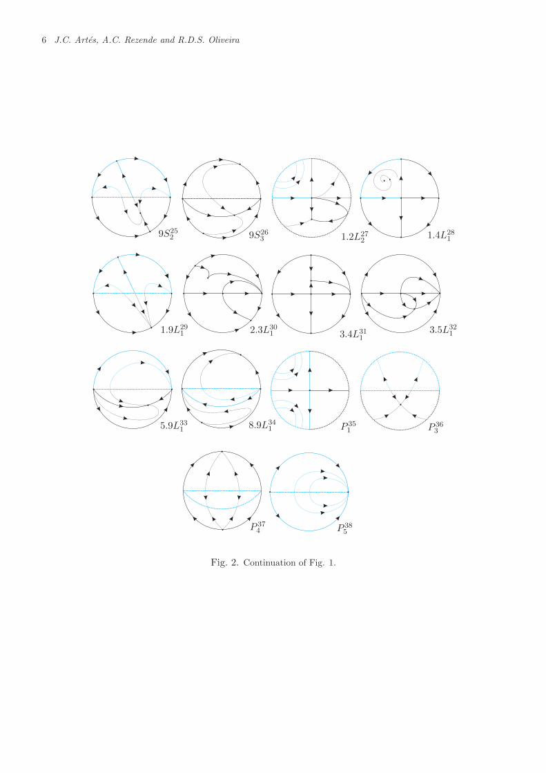
Theorem 1.1. There exist 38 topologically distinctphase portraits for the quadratic vector fields havinga finite saddle–node sn(2) and an infinite saddle–

node of type(02

)SN located in the direction de-

fined by the eigenvector with null eigenvalue (classQsnSN(A)). All these phase portraits are shown inFigs. 1 and 2. Moreover, the following statementshold:

(a) The manifold defined by the eigenvector withnull eigenvalue is always an invariant straightline under the flow;

(b) There exist three phase portraits with limit cy-cles, and they are in the regions V 5

11, V 714 and

1S112 ;

(c) There exist three phase portraits with non-degenerate graphics, and they are in the regions4S19

4 , 7S231 and 1.4L28

1 ;

(d) There exist ten phase portraits with degener-ate graphics, and they are in the regions 9S24

1 ,9S25

2 , 1.2L272 , 1.9L29

1 , 5.9L331 , 8.9L34

1 , P 351 , P 36

3 ,P 374 and P 38

5 ;

(e) Any phase portrait of this family can bifurcatefrom P 35

1 of Fig. 2;

(f) There exist 29 topologically distinct phase por-traits in QsnSN(A).

Theorem 1.2. There exist 25 topologically distinctphase portraits for the quadratic vector fields havinga finite saddle–node sn(2) and an infinite saddle–

node of type(02

)SN located in the direction defined

by the eigenvector with non–null eigenvalue (classQsnSN(B)). All these phase portraits are shownin Fig. 3. Moreover, the following statements hold:

(a) The manifold defined by the eigenvector withnon–null eigenvalue is always an invariantstraight line under the flow;

(b) There exist four phase portraits with non-degenerate graphic, and they are in the regions1S9

4 , 4S101 , 1.4L16

2 and 1.5L171 ;

(c) There exist seven phase portraits with degener-ate graphics, and they are in the regions 1.4L15

1 ,1.9L18

1 , 4.9L191 , P 22

1 , P 232 , P 24

3 and P 255 ;

(d) There exists one phase portrait with a center,and it is in the region 4S10

1 ;

(e) There exists one phase portrait with an inte-grable saddle, and it is in the region 4S1

2 .

(f) Any phase portrait of this family can bifurcatefrom P 22

1 of Fig. 3;

(g) There exist 16 topologically distinct phase por-traits in QsnSN(B).

Corollary 1.3. The phase portrait P 363 from fam-

ily QsnSN(A) in Fig. 2 is equivalent to the phaseportrait P 23

2 from family QsnSN(B) in Fig. 3.Furthermore, the phase portrait 1.2L27

2 from fam-ily QsnSN(A) in Fig. 2 is equivalent to the phaseportrait 1.4L15

1 from family QsnSN(B) in Fig. 3.

For the class QsnSN(A), from its 29 topo-logically different phase portraits, 9 occur in 3–dimensional parts, 14 in 2–dimensional parts, 5in 1–dimensional parts and 1 occur in a single 0–dimensional part, and for the class QsnSN(B),from its 16 topologically different phase portraits,5 occur in 3–dimensional parts, 7 in 2–dimensionalparts, 3 in 1–dimensional parts and 1 occur in asingle 0–dimensional part.

In Figs. 1, 2 and 3 we have denoted all thesingular points with a small disk. We have plot-ted with wide curves the separatrices and we haveadded some orbits drawn on the picture with thin-ner lines to avoid confusion in some required cases.

Remark 1.4. We label the phase portraits accord-ing to the parts of the bifurcation diagram where

4 J.C. Artes, A.C. Rezende and R.D.S. Oliveira

they occur. These labels could be different for twotopologically equivalent phase portraits occurringin distinct parts. Some of the phase portraits in 3–dimensional parts also occur in some 2–dimensionalparts bordering these 3–dimensional parts. An ex-ample occurs when a node turns into a focus. Ananalogous situation happens for phase portraits in2–dimensional (respectively, 1–dimensional) parts,coinciding with a phase portrait on 1–dimensional(respectively, 0–dimensional) part situated on theborder of it.

The work is organized as follows. In Sec. 2 wedescribe the normal form for the families of systemshaving a finite saddle–node and an infinite saddle–

node of type(02

)SN in both horizontal and vertical

axes.

For the study of real planar polynomial vectorfields two compactifications can be used. In Sec. 3we describe very briefly the Poincare compactifica-tion on the 2–dimensional sphere.

In Sec. 4 we list some very basic properties ofgeneral quadratic systems needed in this study.

In Sec. 5 we mention some algebraicand geometric concepts that were introduced in[Schlomiuk et al., 2001, Llibre et al., 2004] involv-ing intersection numbers, zero–cycles, divisors, T–comitant and invariant polynomials for quadraticsystems as used by the Sibirskii school. We re-fer the reader directly to [Artes et al., 2006] wherethese concepts are widely explained.

We construct in Secs. 6 and 7 the algebraicbifurcation surfaces of singularities for the classesQsnSN(A) and QsnSN(B), respectively.

In Sec. 8 we comment about the possible exis-tence of “islands” in the bifurcation diagram.

In Sec. 9 we introduce a global invariant de-noted by I, which classifies completely, up to topo-logical equivalence, the phase portraits we have ob-tained for the systems in the classes QsnSN(A) andQsnSN(B). Theorems 9.11 and 9.12 show clearlythat they are uniquely determined (up to topologi-cal equivalence) by the values of the invariant I.

Remark 1.5. It is worth mentioning that a thirdsubclassQsnSN(C) ofQsnSN must be considered.This subclass consists of planar quadratic systemswith a finite saddle–node sn(2) also situated at theorigin (as we do in this work) and an infinite saddle–

node of type(02

)SN in the bisector of the first and

third quadrants and it is currently being studied.

In [Artes et al., 1998] the authors classi-fied all the structurally stable quadratic pla-nar systems modulo limit cycles, also known asthe codimension–zero quadratic systems (roughlyspeaking, those systems whose all singularities, fi-nite and infinite, are simple, with no separatrixconnection, and where any nest of limit cycles isidentified with the focus inside of them, with thestability of the last limit cycle) by proving theexistence of 44 topologically different phase por-traits for these systems. The natural continua-tion in this idea is the classification of the struc-turally unstable quadratic systems of codimension–one, i.e. those systems which have one and onlyone of the following simplest structurally unstableobjects: a saddle–node of multiplicity two (finite orinfinite), a separatrix from one saddle point to an-other, and a separatrix forming a homoclinic loopwith its divergence non–zero. This study is al-ready in progress [Artes & Llibre, 2013], all topo-logical possibilities have already been found, someof them have already been proved impossible andmany representatives have been located, but thereremain some cases without a candidate. One wayto obtain codimension–one phase portraits is con-sidering perturbations of known phase portraits ofquadratic systems of higher degree of degeneracy.These perturbations would decrease the codimen-sion of the system and we may find a representa-tive for a topological equivalence class in the familyof the codimension–one systems and add it to theexisting classification.

In order to contribute to this classification,we studied some families of quadratic systems ofhigher degree of degeneracy, e.g. systems with aweak focus of second order, see [Artes et al., 2006],and with a finite semi–elemental triple node, see[Artes et al., 2013]. In this last paper, the authorsshow that, after a quadratic perturbation in thephase portrait V11, the semi–elemental triple nodeis split into a node and a saddle–node and the newphase portrait is topologically equivalent to one ofthe topologically possible phase portraits of codi-mension one, expected to exist.

The geometry of quadratic polynomial differential systems with a finite and an infinite saddle–node (A,B) 5

V 11 V 2

3 V 36 V 4

9

V 511 V 6

12 V 714 V 8

15

V 916 1S10

1 1S112 1S12

4

1S135 3S14

1 3S152 3S16

3

3S174

4S181 4S19

1 5S201

5S212 5S22

37S23

1 9S241

Fig. 1. Phase portraits for quadratic vector fields with a finite saddle–node sn(2) and an infinite saddle–node of type(02

)SN in the horizontal axis.

6 J.C. Artes, A.C. Rezende and R.D.S. Oliveira

9S252 9S26

3 1.2L272

1.4L281

1.9L291 2.3L30

1 3.4L311

3.5L321

5.9L331 8.9L34

1 P 351 P 36

3

P 374 P 38

5

Fig. 2. Continuation of Fig. 1.

The geometry of quadratic polynomial differential systems with a finite and an infinite saddle–node (A,B) 7

V 11 V 2

2 V 33 V 4

6 V 57

1S61 1S7

2 1S83 1S9

4 4S101

5S111 5S12

3 9S131 9S14

2 1.4L151

1.4L162 1.5L17

11.9L18

1 4.9L191 5.9L20

1

5.9L212

P 221 P 23

2 P 243

P 254

Fig. 3. Phase portraits for quadratic vector fields with a finite saddle–node sn(2) and an infinite saddle–node of type(02

)SN in the vertical axis.

8 J.C. Artes, A.C. Rezende and R.D.S. Oliveira

The present study is part of this attempt ofclassifying all the codimension–one quadratic sys-tems. We propose the study of a whole familyof quadratic systems having two semi–elementalsaddle–nodes, one finite and one infinite formed bythe collision of two infinite singular points. Bothsubfamilies reported here will not bifurcate to anyof the codimension–one systems still missing, but inthe subfamily QsnSN(C) will appear some new ex-amples due to the highly rich bifurcation diagram,richer than anything we encountered before.

2. Quadratic vector fields with a finitesaddle–node sn(2) and an infinite saddle–

node of type(02

)SN

A singular point r of a planar vector field X in R2

is semi–elemental if the determinant of the matrixof its linear part, DX(r), is zero, but its trace isdifferent from zero.

The following result characterizes the localphase portrait at a semi–elemental singular point.

Proposition 2.1. [Andronov et al., 1973,Dumortier et al., 2006] Let r = (0, 0) be anisolated singular point of the vector field X givenby

x = M(x, y),y = y +N(x, y),

(5)

where M and N are analytic in a neighborhoodof the origin starting with at least degree 2 in thevariables x and y. Let y = f(x) be the solu-tion of the equation y + N(x, y) = 0 in a neigh-borhood of the point r = (0, 0), and suppose thatthe function g(x) = M(x, f(x)) has the expressiong(x) = axα + o(xα), where α ≥ 2 and a 6= 0. So,when α is odd, then r = (0, 0) is either an unsta-ble multiple node, or a multiple saddle, dependingif a > 0, or a < 0, respectively. In the case of themultiple saddle, the separatrices are tangent to thex–axis. If α is even, r = (0, 0) is a multiple saddle–node, i.e. the singular point is formed by the unionof two hyperbolic sectors with one parabolic sector.The stable separatrix is tangent to the positive (re-spectively, negative) x–axis at r = (0, 0) accordingto a < 0 (respectively, a > 0). The two unstableseparatrices are tangent to the y–axis at r = (0, 0).

In the particular case where M and N are real

quadratic polynomials in the variables x and y, aquadratic system with a semi–elemental singularpoint at the origin can always be written into theform

x = gx2 + 2hxy + ky2,y = y + ℓx2 + 2mxy + ny2.

(6)

By Proposition 2.1, if g 6= 0, then we have adouble saddle–node sn(2), using the notation intro-duced in [Artes et al., 2012].

In the normal form above, we consider the co-efficient of the terms xy in both equations factoredby 2 in order to make easier the calculations of thealgebraic invariants we shall compute later.

We note that in the normal form (6) we alreadyhave a semi–elemental point at the origin and itseigenvectors are (1, 0) and (0, 1) which condition thepossible positions of the infinite singular points.

We suppose that there exists a(02

)SN at some

point at infinity. If this point is different from either[1 : 0 : 0] of the local chart U1, or [0 : 1 : 0] of thelocal chart U2, after a reparametrization of the type(x, y) → (x, αy), α ∈ R, this point can be replacedat [1 : 1 : 0] of the local chart U1, that is, at thebisector of the first and third quadrants. However,

if(02

)SN is at [1 : 0 : 0] or [0 : 1 : 0], we cannot

apply this change of coordinates and it requires anindependent study for each one of the cases, whichare not equivalent due to the position of the infinitesaddle–node with respect to the eigenvectors of thefinite saddle–node. See Sec. 3 for the notation.

2.1. The normal form for the subclassQsnSN(A)

The following result states the normal form for sys-tems in QsnSN(A).

Proposition 2.2. Every system with a finitesemi–elemental double saddle–node sn(2) and an in-

finite saddle–node of type(02

)SN located in the direc-

tion defined by the eigenvector with null eigenvaluecan be brought via affine transformations and timerescaling to the following normal form

x = gx2 + 2hxy + ky2,y = y + gxy + ny2,

(7)

where g, h, k and n are real parameters and g 6= 0.

The geometry of quadratic polynomial differential systems with a finite and an infinite saddle–node (A,B) 9

Proof. We start with system (6). This system al-ready has a finite semi–elemental double saddle–node at the origin (then g 6= 0) with its eigenvec-tors in the direction of the axes. The first step is

to place the point(02

)SN at the origin of the local

chart U1 with coordinates (w, z). For that, we mustguarantee that the origin is a singularity of the flowin U1,

w = ℓ+ (−g + 2m)w + (−2h+ n)w2 − kw3 + wz,z = (−g − 2hw − kw2)z.

Then, we set ℓ = 0 and, by analyzing the Jacobianof the former expression, we set m = g/2 in orderto have the eigenvalue associated to the eigenvectoron z = 0 being null and obtain the normal form(7).

In order to consider the closure of the familyQsnSN(A), it is necessary to study the case wheng = 0, which will be discussed later.

Remark 2.3. We note that {y = 0} is an invariantstraight line under the flow of (7).

Systems (7) depend on the parameter λ =(g, h, k, n) ∈ R4. We consider systems (7) whichare nonlinear, i.e. λ = (g, h, k, n) 6= 0. In thiscase, system (7) can be rescaled (x 7→ x/g) andthe parameter space is actually the real projectiveplane RP3, and not R4. The 3–dimensional projec-tive space RP3 can be viewed as the quotient spaceS3 /∼ of S3 by the equivalence relation: (g, h, k, n)is equivalent to itself or to (−g,−h,−k,−n). So,our parameter is [λ] = [g : h : k : n] ∈ RP3 = S3 /∼.Rescaling the time, it suffices to consider the points[g : h : k : n] in this quotient with h ≥ 0. Dueto the symmetry (x, y, t) 7→ (−x,−y, t) we have(g, h, k, n) 7→ (−g,−h,−k,−n). Indeed, after ap-plying the symmetry (x, y, t) 7→ (−x,−y, t) we ob-tain the system

x = −gx2 − 2hxy − ky2,

y = y − gxy − ny2.

This implies that it is sufficient to consider onlyg ≥ 0. Since g2 + h2 + k2 + n2 = 1, then g =√

1− (h2 + k2 + n2), where 0 ≤ h2 + k2 + n2 ≤ 1.We can therefore view the parameter space as

a half–ball B = {(h, k, n) ∈ R3; h2 + k2 + n2 ≤1, h ≥ 0} with base h = 0 and where on the equator

h

h = 0

g = 0

Fig. 4. The parameter space.

two opposite points are identified. When h = 0,we identify the point [g : 0 : k : n] ∈ RP3 with[g : k : n] ∈ RP2. So, the base of the half–ball B(h = 0) can be identified with RP2, which can beviewed as a disk with two opposite points on thecircumference (the equator) identified (see Fig. 4).

For g 6= 0, we get the affine chart:

RP3 \ {g = 0} ↔ R3

[g : h : k : n] 7→ (h

g,k

g,n

g) = (h, k, n)

[1 : h : k : n] 7→ (h, k, n).

The plane g = 0 in RP3 corresponds to theequation h2+k2+n2 = 1 (the full sphere S2) and theline g = h = 0 in RP3 corresponds to the equationk2 + n2 = 1 (the equator h = 0 of S2). However,because of symmetry, we only need half sphere andhalf equator, respectively.

We now consider planes in R3 of the formh = h0, where h0 is a constant. The projectivecompletion of such a plane in RP3 has the equationh− h0g = 0. So we see how the slices h = h0 needto be completed in the ball (see Fig. 5). We notethat when g = 0 necessarily we must have h = 0 onsuch a slice, and thus the completion of the imageof the plane h = h0, when visualized in S3, mustinclude the equator.

The specific equations of the correspondence ofthe points in the plane h = h0 of R3 (h0 a constant)onto points in the interior of S2 (B = {(h, k, n) ∈

10 J.C. Artes, A.C. Rezende and R.D.S. Oliveira

Fig. 5. Correspondence between planes and ellipsoides.

R3; h2 + k2 + n2 < 1}) follows from the bijection:

R3 ↔ B

(h, k, n) ↔(h

c,k

c,n

c

)

with c =

√h2+ k

2+ n2 + 1. That is, for each

plane h = constant in R3 , there corresponds anellipsoid h2(1 + h0)

2/h20 + k2 + n2 = 1 (see Fig. 5).The set defined by g = 0 and h = 1 corresponds

to the open half sphere, while g = 0 = h is theequator of the ball.

In what follows we would have to make a sim-ilar study of the geometry of the different surfaces(singularities, intersections, suprema) involved inthe bifurcation diagram as it has been done in[Artes et al., 2006] or [Artes et al., 2013]. The con-clusion of such a study is that this bifurcation dia-gram has only one singular slice, h = 0, plus a sym-metry h 7→ −h, so that the only needed slices to bestudied are h = 0 (singular) and h = 1 (generic).However, there is a much shorter and easier way todetect the same phenomenon and this comes fromthe next result.

Proposition 2.4. By a rescaling in the variables,we may assume h = 0 or h = 1 in the normal form(7).

Proof. If h 6= 0, we consider the rescaling in thevariables given by (x, y) 7→ (x, y/h) and obtain

x = gx2 + 2xy + kh2 y

2,y = y + gxy + n

hy2.

By recalling the coefficients k/h2 7→ k and n/h 7→n, we obtain system (7) with h = 1. Moreover, wemust also consider the case when h = 0.

2.2. The normal form for the subclassQsnSN(B)

The following result gives the normal form for sys-tems in QsnSN(B).

Proposition 2.5. Every system with a finitesemi–elemental double saddle–node sn(2) and an in-

finite saddle–node of type(02

)SN located in the direc-

tion defined by the eigenvector with non-null eigen-value can be brought via affine transformations andtime rescaling to the following normal form

x = gx2 + 2hxy,y = y + ℓx2 + 2mxy + 2hy2,

(8)

where g, h, ℓ and m are real parameters and g 6= 0.

Proof. Analogously to Proposition 2.2, we startwith system (6), but now we want to place the point(02

)SN at the origin of the local chart U2. By fol-

lowing the same steps, we set k = 0, n = 2h and weobtain the form (8).

For this family, we also study the case wheng = 0 in order to consider the closure of the setQsnSN(B).

Remark 2.6. We note that {x = 0} is an invariantstraight line under the flow of (8).

We construct the parameter space for systems(8) in the same way it was constructed for systems(7), but now with respect to the parameter [λ] =[g : h : ℓ : m] ∈ RP3.

Analogously to the previous family, the bifur-cation diagram for this family in R3 shows only onesingular slice, h = 0, and a symmetry h 7→ −h.Then, only one generic slice needs to be taken intoconsideration, and we choose h = 1, and this alsocan be proved in a much easier way with a trans-formation similar to the previous case as it can beseen in the next result.

Proposition 2.7. By a rescaling in the variables,we may assume h = 0 or h = 1 in the normal form(8).

Proof. If h 6= 0, we consider the rescaling in the

The geometry of quadratic polynomial differential systems with a finite and an infinite saddle–node (A,B) 11

variables given by (x, y) 7→ (x, y/h) and obtain

x = gx2 + 2xy,y = y + ℓhx2 + 2mxy + 2y2.

By recalling the coefficient ℓh 7→ ℓ, we obtain sys-tem (8) with h = 1. Moreover, we must also con-sider the case when h = 0.

3. The Poincare compactification and thecomplex (real) foliation with singulari-ties on CP2 (RP2)

A real planar polynomial vector field ξ can be com-pactified on the sphere as follows. Consider thex, y plane as being the plane Z = 1 in the spaceR3 with coordinates X, Y , Z. The central pro-jection of the vector field ξ on the sphere of ra-dius one yields a diffeomorphic vector field on theupper hemisphere and also another vector field onthe lower hemisphere. There exists (for a proof see[Gonzales, 1969]) an analytic vector field cp(ξ) onthe whole sphere such that its restriction on theupper hemisphere has the same phase curves as theone constructed above from the polynomial vectorfield. The projection of the closed northern hemi-sphere H+ of S2 on Z = 0 under (X,Y,Z) →(X,Y ) is called the Poincare disk. A singular pointq of cp(ξ) is called an infinite (respectively, finite)singular point if q ∈ S1, the equator (respectively,q ∈ S2 \S1). By the Poincare compactification ofa polynomial vector field we mean the vector fieldcp(ξ) restricted to the upper hemisphere completedwith the equator.

Ideas in the remaining part of this sectiongo back to Darboux’s work [Darboux, 1878]. Letp(x, y) and q(x, y) be polynomials with real coeffi-cients. For the vector field

p∂

∂x+ q

∂

∂y, (9)

or equivalently for the differential system

x = p(x, y), y = q(x, y), (10)

we consider the associated differential 1–formω1 = q(x, y)dx−p(x, y)dy, and the differential equa-tion

ω1 = 0 . (11)

Clearly, equation (11) defines a foliation with sin-gularities on C2. The affine plane C2 is com-pactified on the complex projective space CP2 =

(C3 \ {0})/ ∼, where (X,Y,Z) ∼ (X ′, Y ′, Z ′) if andonly if (X,Y,Z) = λ(X ′, Y ′, Z ′) for some complexλ 6= 0. The equivalence class of (X,Y,Z) will bedenoted by [X : Y : Z].

The foliation with singularities defined by equa-tion (11) on C2 can be extended to a foliation withsingularities on CP2 and the 1–form ω1 can be ex-tended to a meromorphic 1–form ω on CP2 whichyields an equation ω = 0, i.e.

A(X,Y,Z)dX+B(X,Y,Z)dY +C(X,Y,Z)dZ = 0,(12)

whose coefficients A, B, C are homogeneous poly-nomials of the same degree and satisfy the relation:

A(X,Y,Z)X +B(X,Y,Z)Y + C(X,Y,Z)Z = 0,(13)

Indeed, consider the map i : C3 \ {Z = 0} → C2,given by i(X,Y,Z) = (X/Z, Y/Z) = (x, y) and sup-pose that max{deg(p),deg(q)} = m > 0. Sincex = X/Z and y = Y/Z we have:

dx = (ZdX −XdZ)/Z2, dy = (ZdY − Y dZ)/Z2,

the pull–back form i∗(ω1) has poles at Z = 0 andyields the equation

i∗(ω1) =q(X/Z, Y/Z)(ZdX −XdZ)/Z2

− p(X/Z, Y/Z)(ZdY − Y dZ)/Z2 = 0.

Then, the 1–form ω = Zm+2i∗(ω1) in C3 \ {Z 6= 0}has homogeneous polynomial coefficients of degreem + 1, and for Z = 0 the equations ω = 0 andi∗(ω1) = 0 have the same solutions. Therefore, thedifferential equation ω = 0 can be written as (12),where

A(X,Y,Z) =ZQ(X,Y,Z) = Zm+1q(X/Z, Y/Z),

B(X,Y,Z) =− ZP (X,Y,Z) = −Zm+1p(X/Z, Y/Z),

C(X,Y,Z) =Y P (X,Y,Z)−XQ(X,Y,Z).(14)

Clearly A, B and C are homogeneous polyno-mials of degree m+ 1 satisfying (13).

In particular, for our quadratic systems (7), A,B and C take the following forms

A(X,Y,Z) =Y Z(gX + nY + Z)

B(X,Y,Z) =− (gX2 + 2hXY + kY 2)Z,

C(X,Y,Z) =Y (2hXY − nXY + kY 2 −XZ).(15)

12 J.C. Artes, A.C. Rezende and R.D.S. Oliveira

and for our quadratic systems (8), A, B and C takethe following forms

A(X,Y,Z) =Z(ℓX2 + 2mXY + 2hY 2 + Y Z),

B(X,Y,Z) =−X(gX + 2hY )Z,

C(X,Y,Z) =X(−ℓX2 + gXY − 2mXY − Y Z).(16)

We note that the straight line Z = 0 is alwaysan algebraic invariant curve of this foliation andthat its singular points are the solutions of the sys-tem: A(X,Y,Z) = B(X,Y,Z) = C(X,Y,Z) = 0.We note also that C(X,Y,Z) does not depend onh.

To study the foliation with singularities definedby the differential equation (12) subject to (13)with A, B, C satisfying the above conditions in theneighborhood of the line Z = 0, we consider thetwo charts of CP2: (u, z) = (Y/X,Z/X), X 6= 0,and (v,w) = (X/Y,Z/Y ), Y 6= 0, covering thisline. We note that in the intersection of the charts(x, y) = (X/Z, Y/Z) and (u, z) (respectively, (v,w))we have the change of coordinates x = 1/z, y = u/z(respectively, x = v/w, y = 1/w). Except for thepoint [0 : 1 : 0] or the point [1 : 0 : 0], the foliationdefined by equations (12),(13) with A, B, C as in(14) yields in the neighborhood of the line Z = 0the foliations associated with the systems

u =uP (1, u, z) −Q(1, u, z) = C(1, u, z),

z =zP (1, u, z),(17)

or

v =vQ(v, 1, w) − P (v, 1, w) = −C(v, 1, w),

w =wP (v, 1, w).(18)

In a similar way we can associate a real foliationwith singularities on RP2 to a real planar polyno-mial vector field.

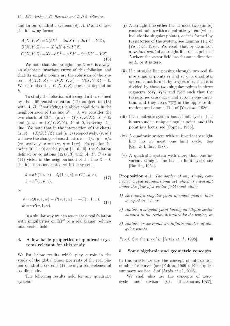
4. A few basic properties of quadratic sys-tems relevant for this study

We list below results which play a role in thestudy of the global phase portraits of the real pla-nar quadratic systems (1) having a semi–elementalsaddle–node.

The following results hold for any quadraticsystem:

(i) A straight line either has at most two (finite)contact points with a quadratic system (whichinclude the singular points), or it is formed bytrajectories of the system; see Lemma 11.1 of[Ye et al., 1986]. We recall that by definitiona contact point of a straight line L is a point ofL where the vector field has the same directionas L, or it is zero.

(ii) If a straight line passing through two real fi-nite singular points r1 and r2 of a quadraticsystem is not formed by trajectories, then it isdivided by these two singular points in threesegments ∞r1, r1r2 and r2∞ such that thetrajectories cross ∞r1 and r2∞ in one direc-tion, and they cross r1r2 in the opposite di-rection; see Lemma 11.4 of [Ye et al., 1986].

(iii) If a quadratic system has a limit cycle, thenit surrounds a unique singular point, and thispoint is a focus; see [Coppel, 1966].

(iv) A quadratic system with an invariant straightline has at most one limit cycle; see[Coll & Llibre, 1988].

(v) A quadratic system with more than one in-variant straight line has no limit cycle; see[Bautin, 1954].

Proposition 4.1. The border of any simply con-nected closed bidimensional set which is invariantunder the flow of a vector field must either

1) surround a singular point of index greater thanor equal to +1, or

2) contain a singular point having an elliptic sectorsituated in the region delimited by the border, or

3) contain or surround an infinite number of sin-gular points.

Proof. See the proof in [Artes et al., 1998].

5. Some algebraic and geometric concepts

In this article we use the concept of intersectionnumber for curves (see [Fulton, 1969]). For a quicksummary see Sec. 5 of [Artes et al., 2006].

We shall also use the concepts of zero–cycle and divisor (see [Hartshorne, 1977])

The geometry of quadratic polynomial differential systems with a finite and an infinite saddle–node (A,B) 13

as specified for quadratic vector fields in[Schlomiuk et al., 2001]. For a quick sum-mary see Sec. 6 of [Artes et al., 2006]. See also[Llibre et al., 2004].

We shall also use the concepts of invariant poly-nomials as used by the Sibirskii school for differen-tial equations. For a quick summary see Sec. 7 of[Artes et al., 2006].

In the next two sections we describe the alge-braic invariants and T–comitants which are relevantin the study of families (7), see Sec. 6, and (8), seeSec. 7.

6. The bifurcation diagram of the systemsin QsnSN(A)

6.1. Bifurcation surfaces due to thechanges in the nature of singularities

For systems (7) we will always have the origin as afinite singular point, a double saddle–node.

From Sec. 7 of [Artes et al., 2008] we get theformulas which give the bifurcation surfaces of sin-gularities in R12, produced by changes that may oc-cur in the local nature of finite singularities. From[Schlomiuk et al., 2005] we get equivalent formulasfor the infinite singular points. These bifurcationsurfaces are all algebraic and they are the follow-ing:

Bifurcation surfaces in RP3 due to multiplic-ities of singularities

(S1) This is the bifurcation surface due to mul-tiplicity of infinite singularities as detected bythe coefficients of the divisor DR(P,Q;Z) =∑

W∈{Z=0}∩CP2 IW (P,Q)W , (here IW (P,Q) de-notes the intersection multiplicity of P = 0 withQ = 0 at the point W situated on the line at infin-ity, i.e. Z = 0) whenever deg((DR(P,Q;Z))) > 0.This occurs when at least one finite singular pointcollides with at least one infinite point. Moreprecisely this happens whenever the homogenouspolynomials of degree two, p2 and q2, in p andq have a common root. In other words wheneverµ = Resx(p2, q2)/y

4 = 0. This is a quartic whoseequation is

µ = g2(gk − 2hn + n2) = 0.

(S3)1 Since this family already has a saddle–

node at the origin, the invariant D, as defined in[Artes et al., 2006], is always zero. The next T–comitant polynomial related to finite singularitiesis T as proved in [Artes et al., 2008]. If this T–comitant polynomial vanishes, it may mean eitherthe existence of another finite semi–elemental point,or the origin being a point of higher multiplicity, orthe system being degenerate. The equation of thissurface is

T = g4(h2 − gk) = 0.

(S5) Since this family already has a saddle–node at infinity, the invariant η, as defined in[Artes et al., 2006], is always zero. In this sense,we have to consider a bifurcation related to theexistence of either the double infinite singularity(02

)SN plus a simple one, or a triple one. This phe-

nomenon is ruled by the T–comitant M as provedin [Schlomiuk et al., 2005, Artes et al., 2012]. Theequation of this surface is

M = 2h− n = 0.

The surface of C∞ bifurcation points due toa strong saddle or a strong focus changingthe sign of their traces (weak saddle or weakfocus)

(S2) This is the bifurcation surface due to weakfinite singularities, which occurs when the trace ofa finite singular point is zero. The equation of thissurface is given by

T4 = g2(−4h2 + 4gk + n2) = 0,

where T4 is defined in [Vulpe, 2011]. This T4 is aninvariant polynomial.

This bifurcation can produce a topologicalchange if the weak point is a focus or just a C∞

change if it is a saddle, except when this bifurcationcoincides with a loop bifurcation associated withthe same saddle, in which case, the change mayalso be topological.

The surface of C∞ bifurcation due to a nodebecoming a focus

1The numbers attached to these bifurcations surfaces donot appear here in increasing order. We just kept the sameenumeration used in [Artes et al., 2006] to maintain coher-ence even though some of the numbers in that enumerationdo not occur here.

14 J.C. Artes, A.C. Rezende and R.D.S. Oliveira

(S6) This surface will contain the points of the pa-rameter space where a finite node of the systemturns into a focus. This surface is a C∞ but nota topological bifurcation surface. In fact, whenwe only cross the surface (S6) in the bifurcationdiagram, the topological phase portraits do notchange. However, this surface is relevant for iso-lating the regions where a limit cycle surroundingan antisaddle cannot exist. Using the results of[Artes et al., 2008], the equation of this surface isgiven by W4 = 0, where

W4 =g4(−48h4 + 32gh2k + 16g2k2 + 64h3n

− 64ghkn − 24h2n2 + 24gkn2 + n4).

Bifurcation surface in RP3 due to the pres-ence of another invariant straight line apartfrom {y = 0}(S4) This surface will contain the points of the pa-rameter space where another invariant straight lineappears apart from {y = 0}. This surface is splitin some regions. Depending on these regions, thestraight line may contain connections of separatri-ces from different saddles or not. So, in some cases,it may imply a topological bifurcation and, in oth-ers, just a C∞ bifurcation. The equation of thissurface is given by

Het = h = 0.

These, except (S4), are all the bifurcation sur-faces of singularities of systems (7) in the parame-ter space and they are all algebraic. We shall dis-cover another bifurcation surface not necessarily al-gebraic and on which the systems have global con-nection of separatrices different from that given by(S4). The equation of this bifurcation surface canonly be determined approximately by means of nu-merical tools. Using arguments of continuity in thephase portraits we can prove the existence of thisnot necessarily algebraic component in the regionwhere it appears, and we can check it numerically.We shall name it the surface (S7).

We shall foliate the three–dimensional bifurca-tion diagram in RP3 by the planes h = 0 and h = 1,given by Proposition 2.4, plus the open half sphereg = 0 and we shall give pictures of the resultingbifurcation diagram on these planar sections on adisk or in an affine chart of R2.

The following two results study the geometricalbehavior of the surfaces, that is, their singularitiesand their intersection points, or the points wheretwo bifurcation surfaces are tangent.

In what follows we work in the chart of RP3

corresponding to g 6= 0, and we take g = 1. Todo the study, we shall use Figs. 7 and 8 whichare drawn on planes h = h0 of R3, h0 ∈ {0, 1},having coordinates (h0, k, n). In these planes thecoordinates are (n, k) where the horizontal line isthe n–axis.

As the final bifurcation diagram is quite com-plex, it is useful to introduce colors which will beused to talk about the bifurcation points:

(a) the curve obtained from the surface (S1) isdrawn in blue (a finite singular point collideswith an infinite one);

(b) the curve obtained from the surface (S2) isdrawn in yellow (when the trace of a singularpoint becomes zero);

(c) the curve obtained from the surface (S3) isdrawn in green (two finite singular points col-lide);

(d) the curve obtained from the surface (S4) isdrawn in purple (presence of an invariantstraight line). We draw it as a continuous curveif it implies a topological change or as a dashedcurve if not.

(e) the curve obtained from the surface (S5) isdrawn in red (three infinite singular points col-lide);

(f) the curve obtained from the surface (S6) isdrawn in black (an antisaddle is on the edge ofturning from a node to a focus or vice versa);and

(g) the curve obtained from the surface (S7) is alsodrawn in purple (same as for (S4)) since bothsurfaces deal with connections of separatricesmostly.

Lemma 6.1. For g 6= 0 and h = 0, no surface, ex-cept (S6), has any singularity and all of the surfacescoincide at [1 : 0 : 0 : 0].

The geometry of quadratic polynomial differential systems with a finite and an infinite saddle–node (A,B) 15

Proof. By setting g = 1 and restricting the equa-tions of the surfaces to h = 0 we obtain: µ = k+n2,T4 = 4k + n2, T = −k, M = −n, W4 = 16k2 +24kn2 + n4 and Het ≡ 0. It is easy too see that µ,T4, T, M and Het have no singularities as they areeither a line, or a parabola, or null. Surface (S6) isa quartic whose only singularity is at [1 : 0 : 0 : 0](this is the union of two parabolas having a com-mon contact point). Besides, if we solve the systemof equations formed by these expressions, we obtain[1 : 0 : 0 : 0] as the unique solution.

Remark 6.2. Everywhere we mention “a contactpoint” we mean an intersection point between twocurves with the same tangency of even order. Ev-erywhere we mention “an intersection point” wemean a transversal intersection point (with differenttangencies).

Lemma 6.3. For g 6= 0 and h = 1, no surface,except (S6), has any singularity. Moreover,

1) the point [1 : 1 : 1 : 0] is a contact point among(S2), (S3) and (S6);

2) the point [1 : 1 : 1 : 1] is a contact point between(S1) and (S3);

3) the point [1 : 1 : 1 : 2] is an intersection pointbetween (S3) and (S5);

4) the point [1 : 1 : 48/49 : 6/7] is an intersectionpoint between (S1) and (S6);

5) the point [1 : 1 : 8/9 : 2/3] is an intersectionpoint between (S2) and (S6);

6) the point [1 : 1 : 0 : −6] is an intersection pointbetween (S4) and (S6);

7) the point [1 : 1 : 0 : −2] is an intersection pointbetween (S2) and (S4);

8) the point [1 : 1 : 0 : 0] is an intersection pointbetween (S1) and (S4);

9) the point [1 : 1 : 0 : 2] is an intersection pointamong all the surfaces, except (S3). Besides,surface (S6) is singular at this point, surface(S4) has a contact point with one of the compo-nents of (S6) and (S1) has a contact point withthe other component of (S6).

Proof. Analogously to the previous lemma, by re-stricting the equations of the surfaces to g = h = 1and solving the system of equation formed by pairsof the restricted expressions, we obtain the re-sult.

Remark 6.4. Even though we are working in RP3,we have seen that the study can be reduced to thegeometry of the curves obtained by intersecting thesurfaces with this slice.

According to Proposition 2.4, we shall studythe bifurcation diagram having as reference the val-ues h = 0 and h = 1 (see Figs. 7 and 8) and alsothe value h = ∞, which corresponds to g = 0. Weperform the bifurcation diagram of all singularitiesfor h = ∞ (g = 0) by putting g = 0 and in the re-maining three variables (h, k, n), yielding the point[h : k : n] ∈ RP2, we take the chart h 6= 0 in whichwe may assume h = 1.

For these values of the parameters, system (7)becomes

x = 2xy + ky2,y = y + ny2,

(19)

and the expressions of the bifurcation surfaces for(19) are given by

µ = T4 = T = W4 = Het = 0

and M = 2− n.(20)

Remark 6.5. We note that {y = 0} is a straightline formed by an infinite number of singularitiesfor system (19). Then, the phase portraits of sucha system must be studied by removing the commonfactor of the two equations defining it and studyingthe linear system that remains. The invariant poly-nomials for linear systems equivalent to the ones forquadratic systems that we use in this paper havenot been defined, but they are trivial to use for aconcrete normal form like (19).

The bifurcation curves of singularities (20) areshown in Fig. 6. We point out that, although wehave drawn in blue the vertical axis k in Fig. 6,it does not represent surface (S1) since it is nullby equations (20), but it has the same geometricalmeaning as this surface, i.e. a finite singular hasgone to infinity.

We now describe the labels used for each part.The subsets of dimensions 3, 2, 1 and 0 of the parti-

16 J.C. Artes, A.C. Rezende and R.D.S. Oliveira

n

k

Fig. 6. Slice of the parameter space for (7) when h = ∞.

n

k

Fig. 7. Slice of the parameter space for (7) when h = 0.

n

k

1s2

1s3

2s2

2s3

2s4

6s2

4s2 4s3 4s4

v4v5

v10

v14

v1

2.3ℓ1

1.4ℓ1

v3

3s1

Fig. 8. Slice of the parameter space for (7) when h = 1.

tion of the parameter space will be denoted respec-tively by V , S, L and P for Volume, Surface, Lineand Point, respectively. The surfaces are namedusing a number which corresponds to each bifurca-tion surface which is placed on the left side of theletter S. To describe the portion of the surface weplace an index. The curves that are intersectionof surfaces are named by using their correspondingnumbers on the left side of the letter L, separatedby a point. To describe the segment of the curve weplace an index. Volumes and Points are simply in-dexed (since three or more surfaces may be involvedin such an intersection). Furthermore, we also adda super–index which will be different for every topo-logically distinct phase portrait. We shall use thissuper–index when related to phase portraits, but wemay skip it while studying the bifurcation diagram.

We consider an example: the surface (S1) splitsinto 6 different two–dimensional parts labeled from1S1 to 1S6, plus some one–dimensional arcs labeledas 1.iLj (where i denotes the other surface inter-sected by (S1) and j is a number), and some zero–dimensional parts. In order to simplify the labelsin Figs. 11 to 13 we see V1 which stands for theTEX notation V1. Analogously, 1S1 (respectively,1.2L1) stands for 1S1 (respectively, 1.2L1). Andthe same happens with other pictures.

Remark 6.6. We point out that the slice h = ∞is a bifurcation surface in the parameter space andreceives the label 9S. We have denoted the curved

The geometry of quadratic polynomial differential systems with a finite and an infinite saddle–node (A,B) 17

segments in which the equator splits as 8.9Lj .

As an exact drawing of the curves produced byintersecting the surfaces with slices gives us verysmall regions which are difficult to distinguish,and points of tangency are almost impossibleto recognize, we have produced topologicallyequivalent pictures where regions are enlargedand tangencies are easy to observe. The readermay find the exact pictures in the web pagehttp://mat.uab.es/∼artes/articles/qvfsn2SN02/qvfsn2SN02.html.

Remark 6.7. We consider g 6= 0. It is worth men-tioning that if we compare the case of the slicesh = 0 and h = 1 (here we may take any otherh > 0), we see that a region looking like a “cross”appears on the slice h = 1 between (S3) (n = 1)and (S4) (n = 0) and also between (S5) (k = 2)and k = 0. This “cross” exists on every slice givenby h > 0 and, as we take h → 0, the region insidethe “cross” including the borders tends to the twoaxes. Furthermore, the rectangle in the middle ofthe cross tends to [1 : 0 : 0 : 0].

We recall that the black surface (S6) (or W4)means the turning of a finite antisaddle from a nodeto a focus. Then, according to the general resultsabout quadratic systems, we could have limit cyclesaround such point.

Remark 6.8. Wherever two parts of equal dimen-sion d are separated only by a part of dimensiond − 1 of the black bifurcation surface (S6), theirrespective phase portraits are topologically equiva-lent since the only difference between them is thata finite antisaddle has turned into a focus withoutchange of stability and without appearance of limitcycles. We denote such parts with different labels,but we do not give specific phase portraits in pic-tures attached to Theorems 1.1 and 1.2 for the partswith the focus. We only give portraits for the partswith nodes, except in the case of existence of a limitcycle or a graphic where the singular point insidethem is portrayed as a focus. Neither do we givespecific invariant description in Sec. 9 distinguish-ing between these nodes and foci.

6.2. Bifurcation surfaces due to connec-tions

We now describe for each set of the partition ong 6= 0 and h = 1 the local behavior of the flowaround all the singular points. Given a concretevalue of parameters of each one of the sets in thisslice we compute the global phase portrait with thenumerical program P4 [Dumortier et al., 2006]. Itis worth mentioning that many (but not all) of thephase portraits in this paper can be obtained notonly numerically but also by means of perturbationsof the systems of codimension one higher.

In this slice we have a partition in 2–dimensional regions bordered by curved polygons,some of them bounded, others bordered by infinity.Provisionally, we use low–case letters to describethe sets found algebraically so as not to interferewith the final partition described with capital let-ters. For each 2–dimensional region we obtain aphase portrait which is coherent with those of alltheir borders, except in one region. Consider theset v1 in Fig. 8. In it we have only a saddle–node as finite singularity. When reaching the set2.3ℓ1, we are on surfaces (S2), (S3) and (S6) at thesame time; this implies the presence of one morefinite singularity (in fact, it is a cusp point) whichis on the edge of splitting itself and give birth tofinite saddle and antisaddle. Now, we consider thesegments 2s2 and 2s3. By the Main Theorem of[Vulpe, 2011], the corresponding phase portraits ofthese sets have a first–order weak saddle and a first–order weak focus, respectively. So, on 2s3 we havea Hopf bifurcation. This means that either in v5or v10 we must have a limit cycle. In fact this oc-curs in v5. Indeed, as we have a weak saddle on2s2 and we have not detected a loop-type bifur-cation surface intersecting this subset, neither itspresence is forced to keep the coherence, its corre-sponding phase portrait is topologically equivalentto the portraits of v4 and v5. Since in v5 we havea phase portrait topologically equivalent to the oneon 2s2 (without limit cycles) and a phase portraitwith limit cycles, this region must be split into twoother ones separated by a new surface (S7) havingat least one element 7S1 such that one region haslimit cycle and the other does not, and the border7S1 must correspond to a connection between sepa-ratrices. After numerical computations we checkedthat the region v5 splits into V5 without limit cycles

18 J.C. Artes, A.C. Rezende and R.D.S. Oliveira

v14

Fig. 9. The local behavior around each of the finite andinfinite singularities of any representant of v14. The redarrow shows the sense of the flow along the y-axis andthe blue points are the focus and the node with samestability.

and V11 with one limit cycle, both of which can beseen in Fig. 13.

The next result assures us the existence of limitcycle in any representative of the subset v14 and itis needed to complete the study of 7S1.

Lemma 6.9. In v14 there is always one limit cycle.

Proof. We see that the subset v14 is characterizedby µ < 0, T4 < 0, W4 < 0, M > 0, T > 0, k > 0and n > 0. Any representative of v14 has the finitesaddle–node at the origin with its eigenvectors onthe axes and two more finite singularities, a focusand a node (the focus is due to W4 < 0). We claimthat these two other singularities are placed in sym-metrical quadrants with respect to the origin (seeFig. 9). In fact, by computing the exact expressionof each singular point (x1, y1) and (x2, y2) and mul-tiplying their x–coordinates and y-coordinates weobtain k/µ and 1/µ, respectively, which are alwaysnegative since k > 0 and µ < 0 in v14. Besides, eachone of them is placed in an even quadrant since theproduct of the coordinates of each antisaddles isnever null and any representative gives a negativeproduct. Moreover, both antisaddles have the samestability since the product of their traces is given byµ/T4 which is always positive in v14.

The infinite singularities of systems in v14 are

the saddle–node(02

)SN (recall the normal form (7))

and a saddle. In fact, the expression of the sin-gular points in the local chart U1 are (0, 0) and((−2h+ n)/k, 0). We note that the determinant of

the Jacobian matrix of the flow in U1 at the secondsingularity is given by

−(2h− n)2(2hn− k − n2

)

k2=

M2µ

k2,

which is negative since µ < 0 in v14. Besides, thispair of saddles are in the second and the fourthquadrant because its first coordinate (−2h+n)/k =

−M/k is negative since M > 0 and k > 0 in v14.

We also note that the flow along the y-axis issuch that x > 0.

Since we have a pair of saddle points in theeven quadrants, each one of the finite antisaddlesis in an even quadrant, no orbit can enter into thesecond quadrant and no orbit may leave the fourthone and, in addition, these antisaddles, a focus anda node, have the same stability, any phase portraitin v14 must have at least one limit cycle in any ofthe even quadrants. Moreover, the limit cycle isin the second quadrant, because the focus is theresince a saddle–node is born in that quadrant at 3s1,splits in two points when entering v3 (both remainin the same quadrant since x1x2 = k/µ < 0 andy1y2 = 1/µ < 0), the node turns into focus at 6s2and the saddle moves to infinity on 1s2 appearing asa node at the fourth quadrant when entering v14.Furthermore, by the statement (iv) of Sec. 4, itfollows the uniqueness of the limit cycle in v14.

Now, the following result states that the seg-ment which splits the subset v5 into the regions V5

and V11 has its endpoints well–determined. We canvisualize the image of this surface in the plane h = 1in Fig. 13.

Proposition 6.10. The endpoints of the part ofthe curve 7S1 are 2.3ℓ1, intersection of surfaces(S2) and (S3), and 1.4ℓ1, intersection of surfaces(S1) and (S4).

Proof. We write r1 = [1 : 1 : 0 : 2] and r2 = [1 :1 : 1 : 0] for 2.3ℓ1 and 1.4ℓ1, respectively. If thestarting point were any point of the segments 2s2or 2s3, we would have the following incoherences:firstly, if the starting point of 7S1 were on 2s2, aportion of this subset must refer to a Hopf bifurca-tion since we have a limit cycle in V11; and secondly,if this starting point were on 2s3, a portion of thissubset must not refer to a Hopf bifurcation which

The geometry of quadratic polynomial differential systems with a finite and an infinite saddle–node (A,B) 19

contradicts the fact that on 2s3 we have a first–order weak focus. Finally, the ending point mustbe r2 because, if it were located on 4s3, we wouldhave a segment between this point and 1.4ℓ1 alongsurface (S4) with two invariant straight lines andone limit cycle, which contradicts the statement (v)of Sec. 4, and if it were on 1s2, we would have asegment between this point and 1.4ℓ1 along surface(S1) without limit cycle which is not compatiblewith Lemma 6.9 since µ = 0 does not produce agraphic.

In Fig. 10 we show the sequence of phase por-traits along the subsets pointed out in Fig. 8.

We cannot be totally sure that this is theunique additional bifurcation curve in this slice.There could exist others which are closed curveswhich are small enough to escape our numerical re-search, but the one located is enough to maintainthe coherence of the bifurcation diagram. We re-call that this kind of studies are always done mod-ulo “islands”. For all other two–dimensional partsof the partition of this slice whenever we join twopoints which are close to two different borders ofthe part, the two phase portraits are topologicallyequivalent. So we do not encounter more situationsthan the one mentioned above.

In Figs. 11 to 13 we show the bifurcation dia-grams for family (7). Since there are two relevantvalues of h to be taken into consideration (accord-ing to Proposition 2.4) plus the infinity, the pic-tures show all the algebraic bifurcation curves andall the non-algebraic bifurcation ones needed for thecoherence of the diagram, which lead to a completebifurcation diagram for family (7) modulo islands.In Sec. 9 the reader can look for the topologicalequivalences among the phase portraits appearingin the various parts and the selected notation fortheir representatives in Figs. 1 and 2. In Fig. 13,we have colored in light yellow the regions with onelimit cycle.

7. The bifurcation diagram of the systemsin QsnSN(B)

Before we describe all the bifurcation surfaces forQsnSN(B), we prove the following result whichgives conditions on the parameters for the presenceof either a finite star node n∗ (whenever any two dis-tinct non–trivial integral curves arrive at the node

with distinct slopes), or a finite dicritical node nd (anode with identical eigenvalues but Jacobian non–diagonal).

Lemma 7.1. Systems (8) always have a n∗, if m =0 and h 6= 0, or a nd, otherwise.

Proof. We note that the singular point (0,−1/2h)has its Jacobian matrix given by

(−1 0

−m/h −1

).

7.1. Bifurcation surfaces due to thechanges in the nature of singularities

The needed invariant and T–comitant polynomialsneeded here are the same as in the previous systemexcept surfaces (S4) and (S6); so we shall only givethe geometrical meaning and their equations plusa deeper discussion on surface (S6). For furtherinformation about them, see Sec. 6.

Bifurcation surfaces in RP3 due to multiplic-ities of singularities

(S1) This is the bifurcation surface due to the multi-plicity of infinite singularities. This occurs when atleast one finite singular point collides with at leastone infinite point. The equation of this surface is

µ = 4h2(g2 + 2hℓ− 2gm) = 0.

(S3) This is the bifurcation surface is due to eitherthe existence of another finite semi–elemental point,or the origin being a higher multiplicity point, orthe system being degenerate. The equation of thissurface is given by

T = −g2h2 = 0.

It only has substantial importance when we con-sider the planes g = 0 or h = 0.

(S5) This is the bifurcation surface due to the col-lision of infinite singularities, i.e. when all three in-finite singular points collide. The equation of thissurface is

M = (g − 2m)2 = 0.

20 J.C. Artes, A.C. Rezende and R.D.S. Oliveira

V 11

2.3L301

6S22 V 2

4

2S22

V 25

7S231

V 511

2S43

V 410

6S43

4S182

V 37

4S183

V 38

1S112

V 714

1.4L281

2S31

2S64

1.2L121

Fig. 10. Sequence of phase portraits in slice g = h = 1 from v1 to 1.8ℓ1. We start from v1. When crossing 2.3ℓ1, wemay choose at least seven “destinations”: 6s2, v4, 2s2, v5, 2s3, v10 and 6s3. In each one of these subsets, but v5, weobtain only one phase portrait. In v5 we find (at least) three different ones, which means that this subset must besplit into (at least) three different regions whose phase portraits are V 2

5 , 7S231 and V 5

11. And then we shall follow thearrows to reach the subset 1.4ℓ1 whose corresponding phase portrait is 1.4L28

1 .

The geometry of quadratic polynomial differential systems with a finite and an infinite saddle–node (A,B) 21

9S1

4.9L1

P2

9S2 9S3

9S4 9S5 9S6

4.9L2 4.9L3

1.9L1 5.9L1

1.9L25.9L2

P3

P5

P4

8.9L1

8.9L2

k

n

Fig. 11. Complete bifurcation diagram of QsnSN(A) for slice h = ∞.

V1

6S1

3.4L1

V2

V6

V7

V8

V15

V17 V22

V21

V20

V19

V18b

2S1

1S1

6S5

5S3

6S6

1S6

2S5

6S7

3.4L25S1P1

k

n

Fig. 12. Complete bifurcation diagram of QsnSN(A) for slice h = 0.

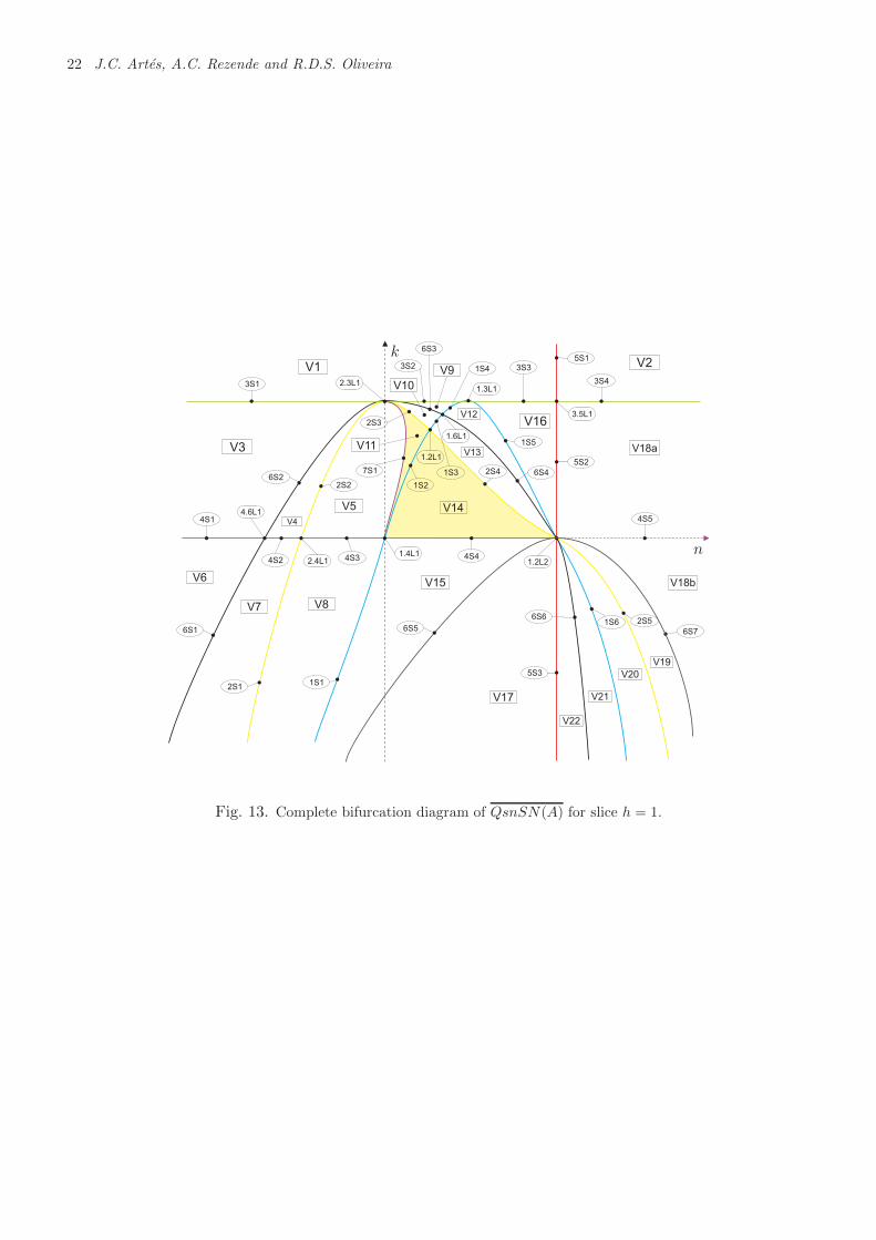
22 J.C. Artes, A.C. Rezende and R.D.S. Oliveira

1S1

4.6L1

V22

V21

V20

V19

V4

V5

V3

V1 V2

V16

V18a

V18b

V14

V15

V8

V6

V7

V17

V11

V10

V9

V12

V13

1S2

1S3

1S4

1S5

1S6

2S1

2S2

2S3

2S4

2S5

3S1

3S2 3S3

3S4

5S1

5S2

5S3

6S1

6S2

6S3

6S4

6S6

6S7

7S1

4S1

4S2 4S3 4S4

4S5

2.4L11.4L1

1.2L2

3.5L1

1.3L12.3L1

1.2L1

1.6L1

6S5

k

n

Fig. 13. Complete bifurcation diagram of QsnSN(A) for slice h = 1.

The geometry of quadratic polynomial differential systems with a finite and an infinite saddle–node (A,B) 23

The surface of C∞ bifurcation due to a strongsaddle or a strong focus changing the sign oftheir traces (weak saddle or weak focus)

(S2) This is the bifurcation surface due to weakfinite singularities, which occurs when their trace iszero. The equation of this surface is given by

T4 = −16h3ℓ = 0.

The surface of C∞ bifurcation due to a nodebecoming a focus

(S6) Since W4 is identically zero for all the bifurca-tion space, the invariant that captures if a secondpoint may be on the edge of changing from node tofocus is W3. The equation of this surface is givenby

W3 = 64h4(g4 + 2g2hℓ+ h2ℓ2 − 2g3m) = 0.

These are all the bifurcation surfaces of singu-larities of the systems (8) in the parameter spaceand they are all algebraic. We do not expect todiscover any other bifurcation surface (neither non-algebraic nor algebraic one) due to the fact that inall the transitions we make among the parts of thebifurcation diagram of this family we find coher-ence in the phase portraits when “traveling” fromone part to the other.

Analogously to the previous class, we shall fo-liate the three–dimensional bifurcation diagram inRP3 by the planes h = 0 and h = 1, given by Propo-sition 2.7, plus the open half sphere g = 0 and weshall give pictures of the resulting bifurcation dia-gram on these planar sections on a disk or in anaffine chart of R2.

The following three results study the geometri-cal behavior of the surfaces, that is, their singulari-ties and the simultaneous intersection points amongthem, or the points where two bifurcation surfacesare tangent, and the presence of a different invari-ant straight line in the particular case when ℓ = 0.

In what follows we work in the chart of RP3

corresponding to g 6= 0, and we take g = 1. Todo the study, we shall use Figs. 15 and 16 whichare drawn on planes h = h0 of R3, h0 ∈ {0, 1},having coordinates (h0, ℓ,m). In these planes thecoordinates are (ℓ,m) where the horizontal line isthe ℓ–axis.

We shall use the same set of colors for the bi-furcation surfaces as in the previous case.

Lemma 7.2. All the bifurcation surfaces intersecton h = 0, with g 6= 0.

Proof. The equations of surfaces (S1), (S2), (S3)and (S6) are identically zero when restricted to theplane h = 0, and the equation of (S5) is the straightline 2m − 1 = 0, for all g 6= 0, h ≥ 0 and m, ℓ ∈R.

Lemma 7.3. For h = 1 (with g 6= 0), the surfaceshave no singularities. Moreover,

1) the point [1 : 1 : −2 : 1/2] is an intersectionpoint between (S5) and (S6);

2) the point [1 : 1 : 0 : 1/2] is an intersection pointamong (S1), (S2), (S5) and (S6). Besides, theintersection between (S1) and (S6) is in fact acontact point.

Proof. For g = h = 1, surface (S1) is the straightline 1 + 2ℓ− 2m = 0, which intersects surface (S5),which is a double straight line with equation −1 +2m = 0, at the point [1 : 1 : 0 : 1/2]; surface(S6) is the parabola 1 + 2ℓ + ℓ2 − 2m = 0 passingthrough the point [1 : 1 : 0 : 1/2] with a 2–ordercontact with surface (S1); moreover, surface (S6)has another intersection point with surface (S5) at[1 : 1 : −2 : 1/2]; surface (S2) is the straight lineℓ = 0, which intersects surfaces (S1), (S5) and (S6)at the point [1 : 1 : 0 : 1/2].

Lemma 7.4. If ℓ = 0, the straight line {y = 0} isinvariant under the flow of (8).

Proof. It is easy to check the result by substitutingℓ = 0 in (8).

According to Proposition 2.7, we shall studythe bifurcation diagram having as reference the val-ues h = 0 and h = 1 (see Figs. 15 and 16) and alsothe value h = ∞, which corresponds to g = 0. Weperform the bifurcation diagram of all singularitiesfor h = ∞ (g = 0) by putting g = 0 and in the re-maining three variables (h, ℓ,m), yielding the point[h : ℓ : m] ∈ RP2, we take the chart h 6= 0 in whichwe may assume h = 1.

For these values of the parameters, system (8)becomes

x = 2xy,y = y + ℓx2 + 2mxy,

(21)

24 J.C. Artes, A.C. Rezende and R.D.S. Oliveira

ℓ

m

Fig. 14. Slice of parameter space for (8) when h = ∞.

and the expressions of the bifurcation surfaces for(21) are given by

µ = 8ℓ, T4 = −16ℓ, T = 0,

M = 4m2 and W3 = 64ℓ2.(22)

Remark 7.5. We note that {y = 0} is a straightline of singularities for system (21) when ℓ = 0.To study the phase portraits of system (21), weproceed as stated in Remark 6.5.

The bifurcation curves of singularities (22) areshown in Fig. 14.

Here we also give topologically equiv-alent figures to the exact drawings ofthe bifurcation curves. The reader mayfind the exact pictures in the web pagehttp://mat.uab.es/∼artes/articles/qvfsn2SN02/qvfsn2SN02.html.

We recall that the black surface (S6) (or W3)means the turning of a finite antisaddle from a nodeto a focus. Then, according to the general resultsabout quadratic systems, we could have limit cyclesaround such focus for any set of parameters havingW3 < 0.

In Figs. 17 to 19 we show the bifurcation dia-grams for family (8). Since there are two relevantvalues of h to be taken into consideration (accord-ing to Proposition 2.7) plus the infinity, the pictures

ℓ

m

Fig. 15. Slice of parameter space for (8) when h = 0.

ℓ

m

Fig. 16. Slice of parameter space for (8) when h = 1.

The geometry of quadratic polynomial differential systems with a finite and an infinite saddle–node (A,B) 25

9S1

5.9L1

P2

4.9L1

9S2

9S49S3

5.9L2

1.9L2

4.9L2

1.9L1

P3

P4

ℓ

m

Fig. 17. Complete bifurcation diagram of QsnSN(B)for slice h = ∞.

show all the algebraic bifurcation curves obtainedby the invariant polynomials. We observe that non-algebraic bifurcation curves were not needed for thecoherence of the diagram. All of these leads to acomplete bifurcation diagram for family (8) mod-ulo islands. In Sec. 9 the reader can look for thetopological equivalences among the phase portraitsappearing in the various parts and the selected no-tation for their representatives in Fig. 3.

8. Other relevant facts about the bifurca-tion diagrams

The bifurcation diagrams we have obtained for thefamilies QsnSN(A) and QsnSN(B) are completelycoherent, i.e. in each family, by taking any twopoints in the parameter space and joining them bya continuous curve, along this curve the changes inphase portraits that occur when crossing the dif-ferent bifurcation surfaces we mention can be com-pletely explained.

Nevertheless, we cannot be sure that these bi-furcation diagrams are the complete bifurcation di-agrams for QsnSN(A) and QsnSN(B) due to thepossibility of “islands” inside the parts bordered byunmentioned bifurcation surfaces. In case they ex-ist, these “islands” would not mean any modifica-

1S5

1.5L2P1

1S4

1S31S6

1.5L3

1.8L1

1.8L2

ℓ

m

Fig. 18. Complete bifurcation diagram of QsnSN(B)for slice h = 0.

1S1

5.6L1

V1

V2

V3V4

V5

V6

V7

V8

V9

1S2

8S1

8S2

5S1

5S2

5S3

1.5L1

6S1

6S3

6S2

ℓ

m

Fig. 19. Complete bifurcation diagram of QsnSN(B)for slice h = 1.

26 J.C. Artes, A.C. Rezende and R.D.S. Oliveira

tion of the nature of the singular points. So, on theborder of these “islands” we could only have bifur-cations due to saddle connections or multiple limitcycles.

In case there were more bifurcation surfaces,we should still be able to join two representativesof any two parts of the 85 parts of QsnSN(A) orthe 43 parts of QsnSN(B) found until now witha continuous curve either without crossing such bi-furcation surface or, in case the curve crosses it, itmust do it an even number of times without tan-gencies, otherwise one must take into account themultiplicity of the tangency, so the total numbermust be even. This is why we call these potentialbifurcation surfaces “islands”.

However, in none of the two families we havefound a different phase portrait which could fitin such an island. The existence of the invariantstraight line avoids the existence of a double limitcycle which is the natural candidate for an island(recall the item (iv) of Sec. 4), and also the limitednumber of separatrices (compared to a generic case)limits greatly the possibilities for phase portraits.

9. Completion of the proofs of Theorems1.1 and 1.2

In the bifurcation diagram we may have topo-logically equivalent phase portraits belonging todistinct parts of the parameter space. As herewe have finitely many distinct parts of the pa-rameter space, to help us identify or to dis-tinguish phase portraits, we need to introducesome invariants and we actually choose integer–valued invariants. All of them were already usedin [Llibre et al., 2004, Artes et al., 2006]. Theseinteger–valued invariants, and sometimes symbol–valued invariants, yield a classification which is eas-ier to grasp.

Definition 9.1. We denote by I1(S) the number ofthe isolated real finite singular points. This invari-ant is also denoted by NR,f (S) [Artes et al., 2006].

Definition 9.2. We denote by I2(S) the sumof the indices of the real finite singular points.This invariant is also denoted by deg(DIf (S))[Artes et al., 2006].

Definition 9.3. We denote by I3(S) the number of

the real infinite singular points. This number canbe ∞ in some cases. This invariant is also denotedby NR,∞(S) [Artes et al., 2006].

Definition 9.4. We denote by I4(S) the sequenceof digits (each one ranging from 0 to 4) such thateach digit describes the total number of global orlocal separatrices (different from the line of infinity)ending (or starting) at an infinite singular point.The number of digits in the sequences is 2 or 4according to the number of infinite singular points.We can start the sequence at anyone of the infinitesingular points but all sequences must be listed ina same specific order either clockwise or counter–clockwise along the line of infinity.

In our case we have used the clockwise sensebeginning from the saddle–node at the origin of thelocal chart U1 in the pictures shown in Figs. 1 and2, and the origin of the local chart U2 in the picturesshown in Fig. 3.

Definition 9.5. We denote by I5(S) a digit whichgives the number of limit cycles.

As we have noted previously in Remark 6.8, wedo not distinguish between phase portraits whoseonly difference is that in one we have a finite nodeand in the other a focus. Both phase portraits aretopologically equivalent and they can only be dis-tinguished within the C1 class. In case we may wantto distinguish between them, a new invariant mayeasily be introduced.

Definition 9.6. We denote by I6(S) the digit 0or 1 to distinguish the phase portrait which hasconnection of separatrices outside the straight line{y = 0}; we use the digit 0 for not having it and 1for having it.

Definition 9.7. We denote by I7(S) the sequenceof digits (each one ranging from 0 to 3) such thateach digit describes the total number of global orlocal separatrices ending (or starting) at a finiteantisaddle.

The next three invariants are needed to classifythe degenerate phase portraits.

Definition 9.8. We denote by I8(S) the index of

The geometry of quadratic polynomial differential systems with a finite and an infinite saddle–node (A,B) 27

the isolated infinite singular point when there ex-ists another infinite singular which is located in theextreme of a curve of singularities.

Definition 9.9. We denote by I9(S) a digit whichgives the number of lines with an infinite numberof singularities.

Definition 9.10. We denote by I10(S) a symbolto represent the configuration of the curves of sin-gularities. The symbols are: “><” to represent ahyperbola, “∪” to represent a parabola and “×” torepresent two crossing lines.

Theorem 9.11. Consider the subfamilyQsnSN(A) which is the closure of all quadraticsystems with a finite saddle–node sn(2) and an

infinite saddle–node of type(02

)SN located in

the direction defined by the eigenvector with nulleigenvalue. Consider now all the phase portraitsthat we have obtained for this family. The values ofthe affine invariant I = (I1, I2, I3, I4, I5, I6, I8, I9)given in the following diagram yield a partition ofthese phase portraits of the family QsnSN(A).

Furthermore, for each value of I in this dia-gram there corresponds a single phase portrait; i.e.S and S′ are such that I(S) = I(S′), if and only ifS and S′ are topologically equivalent.

Theorem 9.12. Consider the subfamilyQsnSN(B) which is the closure of all quadraticsystems with a finite saddle–node sn(2) and an

infinite saddle–node of type(02

)SN located in the

direction defined by the eigenvector with non–nulleigenvalue. Consider now all the phase portraitsthat we have obtained for this family. The valuesof the affine invariant I = (I1, I2, I3, I4, I7, I8, I10)given in the following diagram yield a partition ofthese phase portraits of the family QsnSN(B).

Furthermore, for each value of I in this dia-gram there corresponds a single phase portrait; i.e.S and S′ are such that I(S) = I(S′), if and only ifS and S′ are topologically equivalent.

The bifurcation diagram for QsnSN(A) has 85parts which produce 38 topologically different phaseportraits as described in Tables 1 and 2. The re-maining 47 parts do not produce any new phaseportrait which was not included in the 38 previous

ones. The difference is basically the presence of astrong focus instead of a node and vice versa.

Similarly, the bifurcation diagram forQsnSN(B) has 43 parts which produce 25topologically different phase portraits as describedin Tables 4 and 5. The remaining 18 parts donot produce any new phase portrait which wasnot included in the 25 previous ones. The phaseportraits are basically different to each other undersome algebro–geometric features related to theposition of the orbits.

The phase portraits having neither limit cy-cle nor graphic have been denoted surrounded byparenthesis, for example (V 1

1 ) (in Tables 1 and 4);the phase portraits having one limit cycle have beendenoted surrounded by brackets, for example [V 5

11](in Table 1); the phase portraits having at leastone graphic have been denoted surrounded by {},for example {7S23

1 } (in Table 1).

Proof. The above two results follow from the resultsin the previous sections and a careful analysis ofthe bifurcation diagrams given in Secs. 6 and 7, inFigs. 11, 12, 13, 17, 18 and 19, the definition ofthe invariants Ij and their explicit values for thecorresponding phase portraits.

We first make some observations regarding theequivalence relations used in this paper: the affineand time rescaling, C1 and topological equivalences.

The coarsest one among these three is the topo-logical equivalence and the finest is the affine equiv-alence. We can have two systems which are topo-logically equivalent but not C1–equivalent. For ex-ample, we could have a system with a finite anti-saddle which is a structurally stable node and inanother system with a focus, the two systems beingtopologically equivalent but belonging to distinctC1–equivalence classes, separated by the surface S6

on which the node turns into a focus.

In Table 3 (Table 6, respectively) we listed inthe first column 38 parts (25 parts, respectively)with all the distinct phase portraits of Figs. 1 and2 (Fig. 3, respectively). Corresponding to each partlisted in column 1 we have in its horizontal block, allparts whose phase portraits are topologically equiv-alent to the phase portrait appearing in column 1of the same horizontal block.

In the second column we have put all the partswhose systems yield topologically equivalent phase

28 J.C. Artes, A.C. Rezende and R.D.S. Oliveira

portraits to those in the first column, but whichmay have some algebro–geometric features relatedto the position of the orbits.

In the third (respectively, fourth, and fifth) col-umn we list all parts whose phase portraits haveanother antisaddle which is a focus (respectively, anode which is at a bifurcation point producing fociclose to the node in perturbations, a node–focus toshorten, and a finite weak singular point). In thesixth column of Table 1 we list all phase portraitswhich have a triple infinite singularity with multi-plicity

(21

).

Whenever phase portraits appear on a horizon-tal block in a specific column, the listing is doneaccording to the decreasing dimension of the partswhere they appear, always placing the lower dimen-sions on lower lines.

9.1. Proof of the main theorem

The bifurcation diagram described in Sec. 6, plusTables 1 and 2 of the geometrical invariants distin-guishing the 38 phase portraits, plus Table 3 givingthe equivalences with the remaining phase portraitslead to the proof of the main statement of Theorem1.1. Analogously, we have the proof of Theorem1.2, but considering the description in Sec. 7 andTables 4, 5 and 6.

To prove statements (d) and (e) of Theorem1.2 we recall the Main Theorem of [Vulpe, 2011]and verify that:

(i) Any representative of 4S101 is such that g 6= 0

(we may assume g = 1), h > 0, ℓ = 0 and m >1/2. Then, we have: T4 = 0, T3 = 8h2(2m −1) 6= 0, T3F = −8h4(2m−1)3 < 0, F1 = F2 =F3F4 = 0, which imply that it has a center c;

(ii) Any representative of 4S12 is such that g 6= 0

(we may assume g = 1), h > 0, ℓ = 0 andm < 1/2. Then, we have: T4 = 0, T3 =8h2(2m − 1) 6= 0, T3F = 8h4(1 − 2m)3 > 0,F1 = F2 = F3F4 = 0, which imply that it hasan integrable saddle $.

We observe that the phase portraits 9S252 and

9S263 from family QsnSN(A) are not equivalent to

the phase portrait 4.9L191 from family QsnSN(B)

because the isolated infinite singular point has in-dex 0 in the last phase portrait while its index is

−1 and +1 in the first two phase portraits, respec-tively. Moreover, 9S25

2 and 9S263 are not equivalent

since they are different by the invariant I8.However, the phase portrait P 36

3 from familyQsnSN(A) is equivalent to the phase portrait P 23

2

from family QsnSN(B) since there are no invari-ant that distinguishes them. The same argumentapplies to prove that the phase portrait 1.2L27

2

from family QsnSN(A) is equivalent to the phaseportrait 1.4L15

1 from family QsnSN(B), and thisproves Corollary 1.3.

The geometry of quadratic polynomial differential systems with a finite and an infinite saddle–node (A,B) 29

Table 1: Geometric classification for the subfamily QsnSN(A): the non–degenerate parts.

I1 =

3 & I2 =

2 & I3 =

2 & I4 =

2111 & I5 =

{1 [V 7

14],0 (V 6

12),

1111 & I6 =

{1 {4S19

4 },0 (V 8

15),1 (5S22

3 ),

0 & I3 =

2 & I4 =

4111 & I5 =

{1 [V 5

11],0 (V 4

9 ),

2111 & I6 =

{1 (4S18

1 ),0 (V 3

6 ),3112 (V 2

3 ),2120 (V 9

16),3111 {7S23

1 },1 (5S21

2 ),

2 & I2 =

1 & I3 =

∞ {1.2L272 },

2 & I4 =

2111 & I5 =

{1 [1S11

2 ],0 (1S12

4 ),

1111 & I6 =

{1 {1.4L28

1 },0 (1S10

1 ),2110 (1S13

5 ),

0 & I3 =

2 & I4 =

2111 & I6 =

{1 (3.4L31

1 ),0 (3S17

4 ),3112 (3S14

1 ),4111 (3S15

2 ),2120 (3S16

3 ),3111 (2.3L30

1 ),1 (3.5L32

1 ),

1 & I3 =

∞ {P 351 },

2 (V 11 ),

1 (5S201 ).

Table 2: Geometric classification for the subfamily QsnSN(A): the degenerate parts.

I1 =

1 & I2 =

1 & I3 =

∞ {P 363 },

2 & I8 =

{−1 {9S25

2 },1 (9S26

3 ),1 {5.9L33

1 },−1 {9S24

1 },

0 & I3 =

2 & I8 =

1 & I9 =

{2 {P 37

4 },1 {8.9L34

1 },0 {1.9L29

1 },1 {P 38

5 }.

30 J.C. Artes, A.C. Rezende and R.D.S. Oliveira

Table 3: Topological equivalences for the subfamily QsnSN(A).Presented Identical Finite Finite Finite Triplephase under antisaddle antisaddle weak infiniteportrait perturbations focus node–focus point point

V 11

V 12

1.3L11

V 23

V 24 , V

25

6S22 2S2

2

V 36

V 318a, V

318b V 3

7 , V38 , V

319, V

320

4S35 6S3

1 , 6S37 2S3

1 , 2S35

V 49

V 410

6S43 2S4

3

V 511

V 612

V 613

6S64 2S6

4

V 714

V 815

V 821 V 8

17, V822

6S85 , 6S

86

V 916

1S101 1S10

6

1S112

1S124

1S123

1.6L121 1.2L12

1

1S135

3S141

3S152

3S163

3S174

4S181

4S182 , 4S18

3

4.6L181 2.4L18

1

4S194

5S201

5S212

5S223

7S231

9S241

9S244

4.9L241

9S252

9S255

4.9L252

9S263

9S266

4.9L263

1.2L272

1.4L281

1.9L291

1.9L292

P 292

2.3L301

3.4L311 3.4L31

2

3.5L321

5.9L331 5.9L33

2

8.9L341 8.9L34

2

P 351

P 363

P 374

P 385

The geometry of quadratic polynomial differential systems with a finite and an infinite saddle–node (A,B) 31

Table 4: Geometric classification for the subfamily QsnSN(B): the non–degenerate parts.

I1 =

3 & I2 =

2 & I3 =

2 & I4 =

1111 & I7 =

32 (V 46 ),

31 (V 57 ),

20 {4S101 },

1121 (V 33 ),

1 (5S111 ),

0 & I3 =

2 & I4 =

{2120 (V 2

2 ),1121 {V 1

1 },1 (5S12

3 ),

2 & I2 =

2 & I3 =

{2 (9S13

1 ),1 (5.9L20

1 ),

1 & I3 =

∞ {1.4L151 },

2 & I4 =

{1120 (1S7

2),1111 (1S6

1),

0 & I3 =

{2 (9S14

2 ),1 (5.9L21

2 ),

1 & I3 =

∞ {P 221 },

2 & I4 =

2121 {1S94},

1111 {1.4L162 },

1011 (1S83),

1 {1.5L171 }.

Table 5: Geometric classification for the subfamily QsnSN(B): the degenerate parts.

I1 =

1 & I3 =

{∞ {P 23

2 },2 {4.9L19

1 },

0 & I10 =

>< {1.9L181 },

∪ {P 243 },

× {P 254 },

32 J.C. Artes, A.C. Rezende and R.D.S. Oliveira

Table 6: Topological equivalences for the subfamily QsnSN(B).Presented Identical Finite Finite Finitephase under antisaddle antisaddle weakportrait perturbations focus node–focus point

V 11

V 19

4S12

V 22

V 33

V 34

6S33

V 46

V 45

6S41

V 57

V 58

6S52

1S61

1S72

1S83

1S86

1.4L83

1S94 1S9

5

4S101

5S111

5S112

5.6L111

5S123

9S131 9S13

3

9S142 9S14

4

1.4L151

1.4L162

1.5L171 1.5L17

2

1.9L181 1.5L14

3

4.9L191 4.9L19

2

5.9L201

5.9L212

P 221

P 232

P 243

P 254

The geometry of quadratic polynomial differential systems with a finite and an infinite saddle–node (A,B) 33

Acknowledgements. The first author is partially sup-ported by a MEC/FEDER grant number MTM 2008–03437 and by a CICYT grant number 2005SGR 00550,the second author is supported by CAPES/DGU grantnumber BEX 9439/12–9 and the last author is partiallysupported by CAPES/DGU grant number 222/2010 andby FP7–PEOPLE–2012–IRSES–316338.

References

Andronov, A.A., Leontovich, E.A., Gordon, I.I. & Maier,A.G. [1973] “Qualitative theory of second–order dy-namic systems.” Israel Program for Scientific Trans-lations (Halsted Press, A division of John Wiley &Sons, NY-Toronto, Ontario).

Artes, J.C., Kooij, R. & Llibre, J. [1998] “Structurallystable quadratic vector fields,” Memoires Amer.Math. Soc., 134 (639).

Artes, J.C. & Llibre, J. [2013] “Structurally unsta-ble quadratic systems of codimension 1”, Work inprogress.

Artes, J.C., Llibre, J. & Schlomiuk, D. [2006] “The ge-ometry of quadratic differential systems with a weakfocus of second order,” Internat. J. Bifur. ChaosAppl. Sci. Engrg. 16, 3127–3194.

Artes, J.C., Llibre, J. & Vulpe, N. [2008] “Singularpoints of quadratic systems: a complete classifica-tion in the coefficient space R12,” Internat. J. Bifur.Chaos Appl. Sci. Engrg. 18, 313–362.

Artes, J.C., Llibre, J., Schlomiuk, D. & Vulpe, N.I.[2012] “From topological to geometric equivalencein the classification of singularities at infinity forquadratic vector fields”, Rocky Mountain J. Math.(accepted)

Artes, J.C., Rezende, A.C., & Oliveira, R.D.S. [2013]“Global phase portraits of quadratic polynomial dif-ferential systems with a semi–elemental triple node,”Internat. J. Bifur. Chaos Appl. Sci. Engrg. 23, 21pp.

Bautin, N.N. [1954] “On periodic solutions of a systemof differential equations,” Prikl. Mat. Meh. 18, 128.

Coll, B. & Llibre, J. [1988] “Limit cycles for a quadraticsystem with an invariant straight line and some evo-lution of phase portraits,” Qualitative Theory of Dif-ferential Equations, Colloq. Math. Soc. Janos Bolyai,Bolyai Institut, Szeged, Hungria 53, 111–123.

Coppel, W.A. [1966] “A survey of quadratic systems,”J. Differential Equations 2, 293–304.

Darboux, G. [1878] “Memoire sur les equationsdifferentielles algebriques du premier ordre et du pre-mier degre (melanges),” Bull. Sci. Math. 124A, 60–96, 123–144, 151–200.

Dumortier, F., Llibre, J. & Artes, J.C. [2006] “Qualita-tive Theory of Planar Differential Systems,” Univer-sitext, Springer–Verlag, New York–Berlin.

Dumortier, F., Roussarie, R. & Rousseau, C. [1994]“Hilbert’s 16th problem for quadratic vector fields,”J. Differential Equations 110, 66–133.

Fulton, W. [1969] “Algebraic curves. An introductionto Algebraic Geometry,” W.A. Benjamin, Inc., NewYork.

Gonzalez, E.A. [1969] “Generic properties of polynomialvector fields at infinity,” Trans. Amer. Math. Soc.143, 201–222.

Hartshorne, R. [1977] “Algebraic geometry,” GraduateTexts in Math. 52, Springer.

Hilbert, D. [1900] “Mathematische probleme”, InNachr. Ges. Wiss., editor Second Internat. CongressMath. Paris, 1900, 253–297. Gottingen Math.–Phys.Kl.

Hilbert, D. [1902] “Mathematical problems,” Bull.Amer. Math. Soc. 8, 437–479.

Llibre, J. & Schlomiuk, D. [2004] “The geometry ofquadratic differential systems with a weak focus ofthird order,” Canad. J. Math. 56, 310–343.

Roussarie, R. & Schlomiuk, D. [2002] “On the geometricstructure of the class of planar quadratic differentialsystems,” Qual. Theory Dyn. Syst. 3, 93–122.

Schlomiuk, D. & Pal, J. [2001] “On the geometry inthe neighborhood of infinity of quadratic differentialsystems with a weak focus,” Qual. Theory Dyn. Syst.2, 1–43.

Schlomiuk, D. & Vulpe, N.I. [2005] “Geometry ofquadratic differential systems in the neighborhood ofthe infinity,” J. Differential Equations 215, 357–400.

Vulpe, N.I. [2011] “Characterization of the finite weaksingularities of quadratic systems via invariant the-ory,” Nonlinear Anal. 74, 6553–6582.

Ye, Y.Q. et al. [1986] “Theory of limit cycles,” Trans.of Mathematical Monographs, 66. Amer. Math. Soc.,Providence, RI, 2 edition.