the rodrigues formula and polynomial differential operatorsthe rodrigues formula and polynomial...

JOURNAL OF MATHEMATICAL ANALYSIS AND APPLICATIONS 84, 443482 (1981)

The Rodrigues Formula and Polynomial Differential Operators

RICHARD RASALA

Mathematics Department, Northeastern University, Boston, Massachusetts 021 IS

Submitted by G.-C. Rota

Contents. Introduction. Part A: Known facts on classical polynomials. 1. Three key facts. 2. The adjoint of the derivative operator. 3. An explanation of the three key facts. Part B: Eigenfunctions of polynomial d~flerential operators. 1. Polynomial differential operators. 2. Polynomial eigenfunctions. 3. Useful functions. 4. The Expansion and Inversion Theorems. 5. Recurrence relations. 6. Examples.

This paper began as a study of the role of linear algebra in the theory of the classical orthogonal polynomials of Hermite, Laguerre, and Jacobi. The main theme was the systematic use of adjointness as a means for explaining various formulas. In time, it became clear that

B orthogonality is irrelevant, * for a wide class of polynomial differential operators, there is a

Rodrigues formula to express the polynomial eigenfunctions.

In fact, any polynomial sequence can be generated by a Rodrigues formula. In the general case, the formula is quite complicated.

Part A of the paper is devoted to a sketch of the basic theory of the classical orthogonal polynomials via adjointness. Our aim is to present those ideas from the classical theory which motivated the work of Part B.

The main theorems of the paper are found in Part B where we show that the Rodrigues formula, suitably generalized, can be used to give the polynomial eigenfunctions of certain polynomial differential operators called “regular.” Let PnvA denote these eigenfunctions. Then the high point of the theory is the pair of expansion and inversion theorems which express P,,, in terms of xi/i! and vice versa. The recursive form of these theorems is nicely suited to computer calculations, We are able to use these results to get some facts about recurrence relations as well as to draw out some known formulas for the classical polynomials.

443 0022.247X/81/120443-40802,00/O

Copyright ‘cm 198 1 by Academic Press. Inc. All rights of reproduction in any form reserved.

444 RICHARD RASALA

We now make some brief comments on related work. The inspiration for Part A was the discussion of characterizations of the classical orthogonal polynomials in Magnus et al. [3,5.1.3]. Part A is, in effect, an essay on these characterizations.

Part B grew out of Part A and was inspired to some extent by the beautiful operator calculus of Rota et af. [6, 81. The polynomial sequences we discuss are more general than those of Rota but the expansion and inversion formulas we give are correspondingly more complicated. This work therefore adds to but does not replace the operator calculus of Rota.

The methods of Part B are related to the classical factorization method of Infeld and Hull [ 1] and to the differential-difference method of Truesdell [IO]. The problems treated by these authors are in some ways more general and in some ways less general than those discussed here. A detailed study of the relation of the present paper to these two earlier works would probably be worthwhile.

PART A: KNOWN FACTS ON CLASSICAL POLYNOMIALS

The aim of this part is to recall some known facts about the classical orthogonal polynomials of Jacobi, Laguerre, and Hermite. We will discuss these facts from the point of view which led to the general results of Part B. Since these facts are discussed in many other ways in the literature, we will sketch proofs only when such sketches will be useful in motivating the generalizations to follow.

A. 1. Three Key Facts

The classical orthogonal polynomials of Jacobi, Laguerre, and Hermite have many properties in common but for this study three key facts stand out, namely, the Rodrigues Formula, the Differential Equation, and the Derivative Formula. Before discussing these facts, we introduce some notations.

Let Q,(x) denote the nth degree orthogonal polynomial from one of the classical families. Then the set {Q,} is orthogonal with respect to a scalar product of the form

(f, g>, = f f(-x) g(x) w(x) dx, .lX

where IV(X) is a weight function positive on the interval a < x < b. In the specific cases, we have

RODRIGUES FORMULA 445

Hermite: w(x) = epx2 a=-co, b=+co,

Laguerre: w(x) = xae mx a = 0, b=+co.

Jacobi: w(x) = (1 - x)” (1 + x)4 a=-1, b=+l.

Note that the three cases include all types of interval: infinite, half-infinite, and finite.

When it is important to specify the weight function w(x) in discussing Q,,(x), we will use the longer notation Q,,&,(x).

Let us now consider the Rodrigues Formula. In the specific cases, we have:

Hermite: H,(x) = (-1)” + Dn(emxz),

Laguerre:

Jacobi:

x D”( [ 1 - xZ]n (1 - x)” (1 + x)D).

Here D denotes the derivative with respect to x. If we ignore the scale factors in front, then we can put the Rodrigues Formula into the following general form:

Rodrigues Formula.

Q,(x) = & D"(P(x)l" w(x)).

Here n(x) is the weight function defining the scalar product and A(x) is a polynomial of degree at most 2, specifically:

Hermite: A(x) = 1,

Laguerre: A(x) = x,

Jacobi: A(x) = 1 -x2.

Remark 1. The polynomial ,4(x) is quite important and occurs in several places in the theory. We can characterize A(x) up to a scalar as a polynomial of least degree vanishing on the finite endpoints of the interval of orthogonality.

Remark 2. One can show that the classical weight functions w(x) listed above are characterized up to scalars and affine changes of coordinates as the weight functions such that:

446 RICHARD RASALA

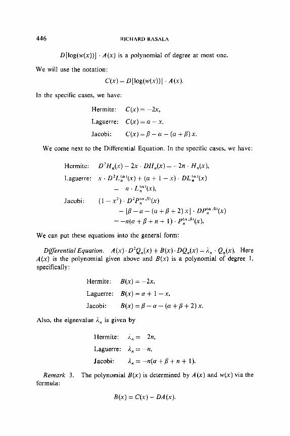
D[log(w(x))] . A(x) is a polynomial of degree at most one.

We will use the notation:

C(x) = D[log(w(x))] . A(x).

In the specific cases, we have:

Hermite: C(x) = -2x,

Laguerre: C(x) = a - x,

Jacobi: C(x)=P-a-(a+P)x.

We come next to the Differential Equation. In the specific cases, we have:

Hermite: D2H,(x) - 2x . DH”(X) = -2n . H,(x),

Laguerre: x . D2Ljp’(x) + (a + 1 -x) . DL5p’(x)

= -n . Lip’(x),

Jacobi: (1 - x?) . DYIp*s’(x)

+ [p - a - (a + p + 2) x] * DPjp.“‘(x)

= -n(a + /I + n + 1) . Pr*4’(x).

We can put these equations into the general form:

DSfferentiul Equation. A(x). D’Q,(x) + B(x). De,,(x) = A, . Qn(x). Here A(x) is the polynomial given above and B(x) is a polynomial of degree 1. specifically:

Hermite: B(x) = -2x.

Laguerre: B(x) = a + 1 -x,

Jacobi: B(x)=p-a-(a-t/3+2)x.

Also, the eigenvalue d,, is given by

Hermite: A, = -2n,

Laguerre: 1, = -n,

Jacobi: A,=--$a+p+n+ I).

Remark 3. The polynomial B(x) is determined by A(x) and M(X) via the formula:

B(x) = C(x) + DA(x).

RODRIGLJES FORMULA 441

Remark 4. If we let p be the coefficient of x2 in A(x) and let 9 be the coefficient of x in B(x), then:

/I,=p*n(n-l)+q*n.

Finally we discuss the Derivative Formula. Of the three facts, this is the most subtle since it sometimes involves a shift in the weight function as we see in the specific cases:

Hermite: DH,(x) = 2n . H,- ,(x),

Laguerre: DLjp’(.x) = -Lr-+r”(?c),

Jacobi: DPyy~) = [(a + p + n + 1)/2] . PlP_:‘,o+“(x).

To obtain a common statement which includes these formulas, we define the weight function adjacent to NV(X) to be W(X) A (x) and we define Q,,, by the version of the Rodrigues formula given above in which there are no special constants. Then we have:

Derivative Formula. DQ,.,(x) = A,,,. . Q,- ,,k..4(x). Here A,., = A, is the eigenvalue given above and Q,- ,,w.A(.~) is the degree n - 1 orthogonal polynomial associated with the adjacent weight function M’(X) A(x).

The rest of Part A will consist of comments on the key facts as a motivation for the work in Part B.

A.2. The Adjoint of the Derivative Operator

One can explain the Rodrigues Formula, the Differential Equation, and the Derivative Formula by using the adjoint of the derivative operator D. The tricky aspect of this explanation is that we need to view D as a map between distinct spaces. We will set up notation to do this.

Let P denote the vector space of polynomials and let P, be the subspace of P consisting of polynomials of degree at most n. When we wish to view P with a scalar product defined by a weight function u, we will use the notations P,. and P,,,,.

The Derivative Formula suggests that we view the derivative D as a map

D: P,.+ P,.,4. Then the desired adjoint is a map

D*: P,,.,4 +,P,,, such that for all polynomials f,g:

Wg),.., = (L D*g),.

448 RICHARD RASALA

It turns out that because A(x) vanishes at the finite endpoints of the interval of orthogonality the computation of D* is especially simple. The result can be expressed in two ways:

Adjoint Formula 1. For any polynomial g,

(D*g)(x) = - &W) w(x)A(~)I.

Adjoint Formula 2. For any polynomial g,

@‘*g)(x) = - [A(x) Q(x) + B(x) &)I.

Adjoint Formula I follows by a standard argument using integration by parts. Adjoint Formula 2 then follows by applying the product rule and observing that

= D[log(w(x))] . A(x) + DA(x)

= C(x) + DA(x) = B(x).

As a consequence of Adjoint Formula 2 and the fact that A(x) and B(x) are polynomials of degrees 2 and 1, respectively, we have:

Remark 1. For any polynomial g, D*g is also a polynomial and

Degree(D*g) < Degree(g) + 1.

For any integer n, we can now view D and D* as a pair of adjoint maps between finite dimensional spaces of polynomials:

D:P n+,.w+Pn.w...,r D*:Pn,,u..~+“,+,,,..

Now, for all n, D is surjective so, by adjointness, D* is injective, for all n. This means simply that:

Remark 2. D* is injective.

Finally, the kernel of D is the constant polynomials, so likewise:

Remark 3. The self-adjoint operator D*D: P,,, + P, has kernel consisting of the constant polynomials.

Change of Notation. To eliminate the frequent occurrence of minus signs


and to include the dependence of the adjoint on n(x) in the notation, we define operators E,, and S,. by the formulas:

E,,.g = -D*g, S,f = -D*Df = E,,,DJ

We use this notation in the next section.

A.3. An Explanation of the Three Key Facts

The Rodrigues Formula asserts that a suitable choice for the nth orthogonal polynomial Q,,,. is

Q,,,&) = &D”[w(x) . A(x)“].

We will first explain why this is true. We may view Qll.,,,(x) as a polynomial spanning the orthogonal

complement of P, _, .,~ in Pn.w:

(Q,.,) = lPn-,.,,~lL within P,,,,..

However, P, _, is the kernel of the nth power D”: P, --) P, of the derivative map D. Thus, by a fundamental fact on adjointness:

(Q,,,.) = [Kernel(D = Image((D”)*).

Here: (D”)*: P, + P,. We will see that the Rodrigues Formula says that Q,,,,, is the value of (D”)* on a suitable constant polynomial.

To make this explicit, recall that, for purposes of computing the adjoint. we viewed D as a map between distinct spaces:

D: P,. + P,,.., .

Thus we must view D” as the composite:

P &&$.A Pn-,.+.4 a pn&&y/+ *** --% PO.$...~“.

The image of the adjoint (D”)* of this composite will give the desired orthogonal complement of P,-, in P,. The adjoint (D”)* equals the following composite up to the sign factor (-1)“:

450 RICHARD RASALA

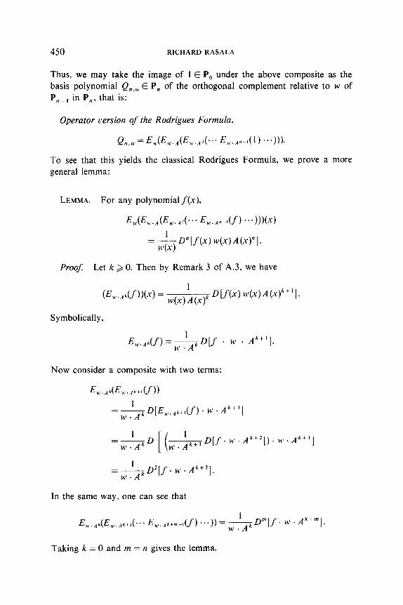
Thus, we may take the image of 1 E P, under the above composite as the basis polynomial Q,,, E P, of the orthogonal complement relative to w of P ,, _, in P,, that is:

Operator cersion of the Rodrigues Formula.

Q,.,c = E,.(E I,... d(Ew..A:(... E 111.. p,(l) ..e))).

TO see that this yields the classical Rodrigues Formula, we prove a more general lemma:

LEMMA. For any polynomial f(x),

E,,.(E,,..A(EH...~?(... Ew.4” 07 -.-))W)

=-&www4x)“l.

ProoJ Let k > 0. Then by Remark 3 of A.3, we have

(E,...d/-))(,u) = ,c(x)j4(x)x D[f(x) 4GW”“l~

Symbolically,

E,,...Af) =A D[f . u’ . Ak+‘].

Now consider a composite with two terms:

E,..,&,,...~k+~df))

= &$[E,,..,4~+,(.f) . IV . Ak+ ‘1

1 =yD

WV . A K M,.;k+,D[f. wAkf2]). M’.Ak+‘]

= &D*[f. M-. A”+‘].

In the same way, one can see that

Taking k = 0 and m = n gives the lemma.


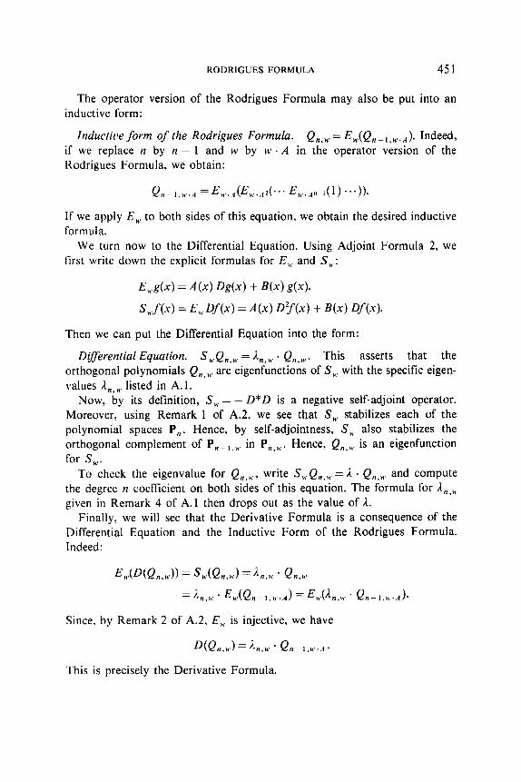
The operator version of the Rodrigues Formula may also be put into an inductive form:

Inductice form of the Rodrigues Formula. Q,,, = E,(Q,- ,,,..,.,). Indeed, if we replace n by n - 1 and w by 1~ . A in the operator version of the Rodrigues Formula, we obtain:

Qn- L.,, ‘.,I =E,..,4(E W’. 44.e. E ,,‘., ,n-l(1) e..)).

If we apply E,. to both sides of this equation, we obtain the desired inductive formula.

We turn now to the Differential Equation. Using Adjoint Formula 2, we first write down the explicit formulas for E, and S,.:

E,.&) = A(x) h(x) + B(x) &).

S,,.f(x) = E,,.Df(x) = A(x) DIf(x) + B(x) Of(x).

Then we can put the Differential Equation into the form:

D@v-ential Equation. S,.Q,.,. = A,,,. . Q,,,. This asserts that the orthogonal polynomials Q,,,,. are eigenfunctions of S,. with the specific eigenvalues A,, ~ listed in A. 1.

Now, by its definition, S,, = - D*D is a negative self-adjoint operator. Moreover, using Remark 1 of A.2, we see that S,. stabilizes each of the polynomial spaces P,. Hence, by self-adjointness, S, also stabilizes the orthogonal complement of P, _, . )I in P,,,.. Hence, Q,,, is an eigenfunction for S,.

To check the eigenvalue for Q,,,, write S,,,Q,,,. =A . Q,,w and compute the degree n coefficient on both sides of this equation. The formula for An-W given in Remark 4 of A.1 then drops out as the value of i.

Finally, we will see that the Derivative Formula is a consequence of the Differential Equation and the Inductive Form of the Rodrigues Formula. Indeed:

EwWQ,.,)) = sJQ,,J = Lw . Qw

= L,, * Ew.(Qn-,.,,,.A) =EdLw . Qn-,.,..A)-

Since. by Remark 2 of A.2, E,< is injective, we have

D(Q,.,J = k,,, . Qn- ,.,<..4.

This is precisely the Derivative Formula.

452 RICHARD RASALA

PART B. EIGENFUNCTIONS OF POLYNOMIAL DIFFERENTIAL OPERATORS

The main theme of the theory to be developed below is that the Rodrigues Formula suitably generalized can be used to pick out the polynomial eigenfunctions of a wide class of polynomial differential operators. We obtain pretty formulas for the coefficients of the eigenfunctions P,(x) in terms of polynomials x’/i! and inversely for xi/i! in terms of P,,(x). These formulas can be put in a recursive form which is quite nice for computer calculation.

B. 1. Polynomial Differential Operators

Let A = (A@, A,, A2 . . . . . A,,, ,..., ) denote a sequence of polynomials. Define the polynomial differential operator S, associated with A by

(S,fK~)= 5 A,(x). D"f(xh m-0

Notice that this operator is well defined on any polynomial f since D"f = 0 for m 9 0. Moreover:

LEMMA 1. Let T: P + P be a linear operator or1 the space P of po!vnomials. Then T = .S4 for a unique sequence A of polynomials.

Proof. By induction, we can define A,(x) uniquely from the equation

m T(xm) = S, (xm) = =K- A&) . Dk(x”).

k:O

Then, T and S, agree on a basis of P, and therefore, agree on P. One consequence of the lemma is that the theory of polynomial differential

operators coincides with the theory of all operators. Thus, to study eigenfunction questions, for example, one must make some restrictions on the class of PDO’s considered. Let us discuss the restrictions we will make. Let

and

M, = is,.k/.

Then M, is the matrix of S,4 relative to the basis 1, x ,..., -yn ,..., of P. We have little hope of finding the eigenfunctions of M, unless M, has some special properties. The properties we will assume are


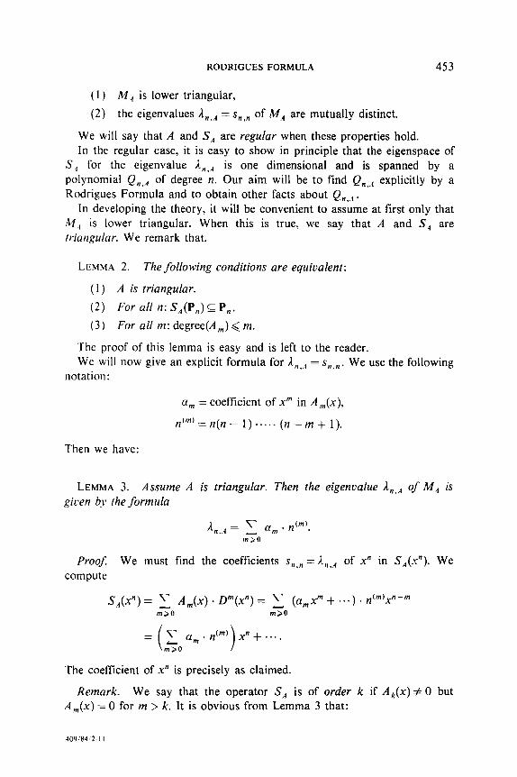
( 1) M,, is lower triangular,

(2) the eigenvalues ln,A = s,,, of M,4 are mutually distinct.

We will say that A and S, are regular when these properties hold. In the regular case, it is easy to show in principle that the eigenspace of

S, for the eigenvalue l,,A is one dimensional and is spanned by a polynomial Q,.,4 of degree n. Our aim will be to find Qn,,4 explicitly by a Rodrigues Formula and to obtain other facts about Q,,,,.

In developing the theory, it will be convenient to assume at first only that 121, is lower triangular. When this is true, we say that A and S, are triangular. We remark that.

LEMMA 2. The following conditions are equivalent:

(1) A is friangular.

(2) For all n: S,(P,) c P,. (3) For all m: degree(A,) < m.

The proof of this lemma is easy and is left to the reader. We will now give an explicit formula for A,, = s,.,. We use the following

notation:

u, = coefficient of x”’ in A,(x),

n lm)=n(n- 1) ....- (n - m + 1).

Then we have:

LEMMA 3. Assume A is triangular. Then the eigenvalue L,,,4 of M, is given by the formula

/1,.,4 = x a, . ntm’. m>O

Proof: We must find the coefficients s,,, =AnqA of x” in S,(P). We compute

SA(Xn) = x A,(x). D”(x”) = x (a,xm + . ..) . n(m’xn-m m>O m>O

= \‘ a, . n’“’ ?ZO

xn + . . . .

The coefficient of x” is precisely as claimed.

Remark. We say that the operator S, is of order k if Ak(x) # 0 but A,(x) = 0 for m > k. It is obvious from Lemma 3 that:

409 :a4 ;2 I I

454 RICHARD RASALA

If S,4 is of order <k, then u, = 0 for m > k and so L,.,4 is a polynomial in n of degree at most k.

In particular, when S,4 is of finite order, then in principle one can check in a finite number of steps whether the eigenvalues L,,,4 are mutually distinct.

B.2. Polynomial Eigenfunctions

Throughout, we let A = (A,,, A,, A, ,..., A, ,...,) denote a triangular sequence of polynomials, that is, such that

degree(A,) < m.

We maintain the other notation of Section B.1 and we seek polynomial eigenfunctions of S,, .

In the study of classical orthogonal polynomials in Part A, we found it important to introduce the weight function adjacent to a given weight function. Here, we must introduce the sequence LA adjacent to a given sequence A :

LA=(A,+DA,,A,+DA,,A>+DA, ,..., A,+DA,+ ,,.... ).

Equivalently, LA=(I+d)A,

where I is the identity operator on sequences and

Note that

6A = (DA,, DA?, DA, ,..., DA,, ,,..., ).

A triangular 3 LA triangular.

We will also need an operator E, to play the role in this theory that was played by E,, in the classical case. We define

(E, f) = f A,(x) . D” - ‘j-(x). m=l

We then take the inductive form of the Rodrigues Formula as the definition of the polynomials Qn,A, that is, we set

Qo,.~ = 1,

Qn..d =EACQn-,.,..t).

We can now state the fundamental theorems:

DIFFERENTIAL EQUATION THEOREM. S,(Q,.,)=k,,, . Q,,,,.

DERIVATIVE THEOREM. D<Q,,.,) = L&z.., - &,,d 1 . Qn- l.c.4 .


Before the proofs of these theorems, we make some remarks:

Remark 1. We emphasize that the fundamental theorems hold when A is triangular. However, we will later need the assumption that A is regular to show that, for all n, degree@,.,) = n.

Remark 2. The Derivative Theorem has a slightly different form than in the classical case because S, is now allowed to have the term A,(x). Note that, in the notation of Lemma 3 of Section B.l

A,(x) = a0 = A”,*, .

We now give two lemmas which we need later. The first lemma is easy and its proof will be omitted.

LEMMA 1. Operator identities.

(1) S,=E,~D+~o.a.

(2) S,, = D . E, + 1o.A.

(3) SL.4 . D = D . S,4 .

LEMMA 2. For all k: ,l,.,,4 = &+ ,.A.

Prooj: The mth polynomial in LA is A,(x) + DA,, ,(x) and the coefficient of .P in this polynomial is

a,+(m+ l).am,,.

Thus.

1 k,LA = y [a,+(m+ l)~a,+,l.k’“’ mT0

=va. L m kcm’ + c a, . m . ktrnmL) ma0 ItI>,

= V a - m . (kc”” + m . k(mp”]a m>O

We compute the term in brackets:

k’m)+m.k’“-“=k . . . . . (k-m+ l)+m .k . . . . . (k-m+2)

=k ----a (k-mf2). [k-m+ l+m]

= (k + 1). k . . . . . (k - m + 2) = (k + I)‘“‘.

Thus.

A k.LA = x am * (k+ l)(m’=&+,,r. ffl>O

456 RICHARD RASALA

We are now ready for:

Proofs of the Fundamental Theorems

For the moment, we fix n and we introduce abbreviations for the two assertions we wish to show:

DET,: For all triangular polynomial sequences A:

S.4 (Qc.4 1 = J-n..4 . en..., .

DT,,: For all triangular polynomial sequences A:

WQ,.A) = IL.., - 4m 1 . Qn- I.L..~ .

The needed proofs will then be accomplished by three steps:

Step 1. DET, is true.

Step 2. For n> l:DET,_,+DT,,.

Step 3. For n> l:DT,+DET,.

Proof of Step 1. Since QD,,4 = 1 is constant, we have

s,(Q,,.A) = (E, D + &.A )(Qo..r ) = JOLT . Qw .

Proof of Step 2.

Proofof Step 3.

S,JQn,A) = FA . D + &,.,)(Q,..A)

= ~,W?n,.,~, + &,.A * Qn...,

=c,(Pn,.~ -&,,I . Qn-I,LA) + A,,, . Qn.,

= LA -&,,I e EA(Qn-,,I..#) + h,,, . en..,

= L.4 . Q".A.

by definition

by Lemma I

by DET, . ,

by Lemma 2.

by Lemma I

by DT,

by definition.


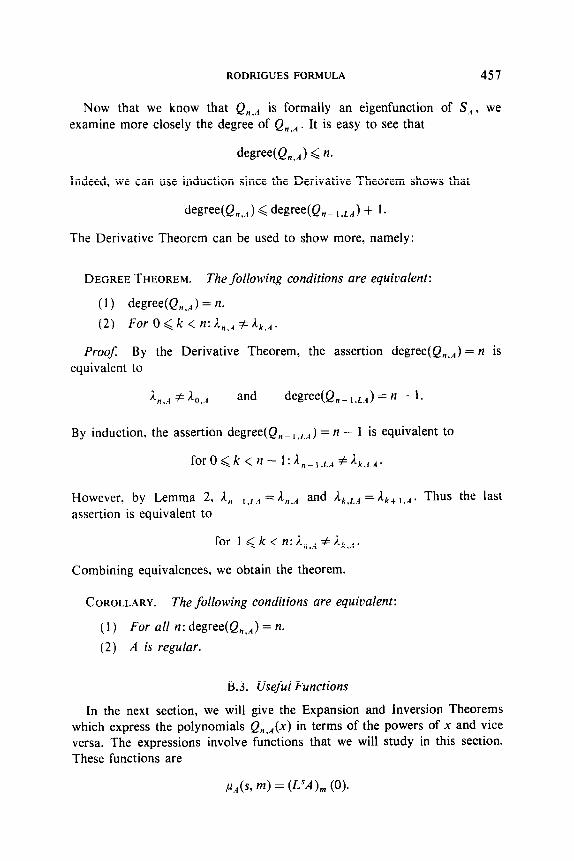
Now that we know that Qn,A is formally an eigenfunction of S,4, we examine more closely the degree of Q,,,4. It is easy to see that

degree(Q,,,) < n.

Indeed, we can use induction since the Derivative Theorem shows that

dewe(Q,,,) < dwee(Q,- I,LA) + 1.

The Derivative Theorem can be used to show more, namely:

DEGREETHEOREM. The following conditions are equivalent:

( 1) degree(Q,,,) = ‘1. (2) ForO<k<n:A,,,#i,,,.

Proof By the Derivative Theorem, the assertion degree(Q,,,) = n is equivalent to

and degree(Q, - , ,L.4) = n - 1.

By induction. the assertion degree(Q, _, .L,,) = n - 1 is equivalent to

However, by Lemma 2, An-,.L,4 = A,,, and Ak ,,-, 4 = Ak+ ,.A. Thus the last assertion is equivalent to

for 1 < k < n: An.* #ilk,,., .

Combining equivalences, we obtain the theorem.

COROLLARY. The following conditions are equivalent:

(1) For all n: degree(Q,,,) = n.

(2) A is regular.

B.3. Useful Functions

In the next section, we will give the Expansion and Inversion Theorems which express the polynomials Q,,,(x) in terms of the powers of x and vice versa. The expressions involve functions that we will study in this section. These functions are

P.~(s, m> = (LsA),n (0).

458 RICHARD RASALA

In words,

p,,(s, m) = constant term of the mth polynomial in the

polynomial sequence L”A.

We will see why these functions are important later. An immediate consequence of the definition is:

LEMMA 1. Iup/& m) =Iu4(s + & m).

To obtain explicit formulas for ~,~(s. m), we must introduce notation for the coefficients of the polynomials A,(x). With hindsight, a good notation is

Then:

LEMMA 2. P,~(s, m) = x:,>o s”) a a,,,+,.,.

Proof: First,

L’A=(I+@‘A= 1 ‘; 0

. S’A. I>0

Now, the mth polynomial in the sequence &A is D’A,+t(.u). Thus

W’A), (x) = x (;) . D’A,+,(x). f>O

The coeflkient of x’ in A,+,(x) is a,+l,m. Hence, the constant term in D’A,+,(x) is

Thus,

t! a lTl+t.Vl*

,a,.,@, m) = (La),,, (0) = z: 0 ; . ~‘A,,,+,~O) I>0

\’ s”’ . a m+t,m= - m+t.WZ f>O Remark 1. The coeffkient of x”’ in A,(x) is a, in the notation of

Lemma 3 of Section B. 1 and is a,,, here. Comparing the lemmas, we see that


With this observation, Lemma 2 of Section B.2 is a special case of Lemma 1 above.

Remark 2. In hand calculations, a slightly different notation for the coefficients of the A,(x) is sometimes convenient:

A,(x)=a, *x+/3,,

AZ(X) = (12 . x2 + p2 . x + y2,

A,(.u)=a,.?c3+p,.xZ+y,.x+6,.

With this notation, we can write down some explicit examples of the values P., (s, m):

s=o s=l s=2 s=3

m=O a0 ao+a, a,+2a, +2a, a, + 3a, + 6a, + 6a3

m=l /?, la, + P2 PI + 332 + 2& P, + 3P, + 6P, + 6P4

m=2 Y2 Y2 + 73 72 + 273 + 2Y, ~2 + 373 +Q, + 67,

If we think of the coefftcients of the polynomials A,(x) as in layers from the top down, that is, a-layer, b-layer, y-layer, etc., we see that any value ~,~(s, m) involves coefficients from exactly one layer.

Remark 3. The function P,,, can be used to compute the entries in the matrix M, = Is~,~~ of the operator S,. Since we do not need the result explicitly, we simply state the answer:

LEMMA 3. snek = n’n-k) . p,(k, n - k).

B.4. The Expansion and inversion Theorems

We now assume throughout that the polynomial sequence A is regular. We wish to expand Q, ,l(x) in terms of powers of x and then invert these formulas to obtain the powers of x in terms of the polynomials ensA( With hindsight, the formulas simplify if we work with

n-l P,..Jx) = Qn&)/ n (L, - L.4)

k=O 1 and

xi/i!

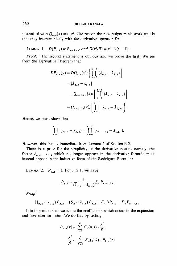
460 RICHARD RASALA

instead of with Q,,,(x) and xi. The reason the new polynomials work well is that they interact nicely with the derivative operator D:

LEMMA 1. D(P,,,) = Pn-,,LA and D(x’/i!) =x-‘/(i - l)!

Pro05 The second statement is obvious and we prove the first. We see from the Derivative Theorem that

Hence, we must show that

However, this fact is immediate from Lemma 2 of Section B.2. There is a price for the simplicity of the derivative results, namely, the

factor kL.4 - lo,, which no longer appears in the derivative formula must instead appear in the inductive form of the Rodrigues Formula:

LEMMA 2. Po,,d = 1. For n >, 1. we have

Proof:

(LA -~o,,)PL4 = (S/l -~o..‘t)Pn..4 =E,DPn./l =E4Pn-I.L.4.

It is important that we name the coefficients which occur in the expansion and inversion formulas. We do this by setting

xj

- = + K,.,(j, k) . P&J(X). j! kr0


We can now state the Expansion and Inversion Theorems:

EXPANSIONTHEOREM. C,(n, n) = 1. For i < n, C,(n, i) can be given in either of two ways:

( 1) Recursive Formula.

1

L

n i

Ch 4 = (n,.A -Aia,4) *z, lu,(i, m). C,4(n, i + m) ; I

(2) Explicit Formula. We have

where the sum is taken over all systems of integers M = (m, ,..., m,) such that

m, f... +m,=n-i. m,>l,r>l

and where we use the notation t,=i+ x mP.

PC4

INVERSIONTHEOREM. KA(j,j) = 1. For k cj, K,(j, k) can be given in either of two ways: ’

(1) Recursive Formula.

1

K‘4uy k, = (&, - Aj,A) pA(j - m, m) . K,4(j - m, k) .

I

(2) Explicit Formula. We have

where the sum is taken over all systems of integers M = (m, ,..., m,) such that

m, +...+m,=j-k, m,> l,r> 1

and where we use the notation

t,= k+ \‘ mP. PC4

Let us immediately give some examples, making use of Remarks 1 and 2 of Section B.3.

462

EXAMPLE 1.

EXAMPLE 2.

EXAMPLE 3.

RICHARD RASALA

Pu,(O, 1) P, P,,,(x) =x + (A,.,, _ Ao.-l) . 1 =x + c(l’

Pu,(O- 1) x = PL.4(X) + (lo,,4 _ A,,,) . Po,.4(x)

= p, ,.4(x) - 5 . Po.,(-y).

P,,,(x) = z + iu.Sl. 1) 2 bL.4 -A,,) . x

ill.4(0, l)Pu,(l, 1) Pu,(O? 2)

@2..4 -~0,,@2.d -n,..41+ CL4 -Jo.,) . l 1 -x2 I P, +P2

2 a, +2az .x

+ P,do, +Pz) + Y2 2(a, + %)(a, + 2u2) 2(a, + a,) ’

EXAMPLE 4.

+ ,u,m l)Pu,(l, 1) PUA (07 2) Go., - ~,.,4>(~0,.4 - Ll) + @0,.4 - h.4) I . pod(x)

a0 - 2(a, + a2) - 2(a, + a,) I * PO.,(X).

We now give:

Proofs of the Expansion and Inversion Theorems.

Step 1. Simple identities


LEMMA 3. For n > i > 0 and j > k > 0, we have

C,(n, i) = Crlr(n - 1, i - 1) = ... = Cri,4(n -i, 0).

K,4 (j, k) = KLA(j - 1, k - 1) = ... = KLk,d( j - k, 0).

Proof. We show, for example, that C,4(n, i) = C,,d(n - 1, i - 1). To do this. we differentiate the expansion formula for P,.,d(x), using Lemma 1:

Comparing this formula with the expansion for Pn-,,LA given by definition, we obtain the desired identity.

One consequence of Lemma 3 is that

C,4(% n) = C,“,(O, 0) = P,,pA(o) = 1.

Step 2. The Recursive Formula for C,d(n, i)

We begin with a special case, namely, C,(t, 0). Using Lemmas 1 and 2, we see that

@,,A - &,A) * PI.A(X) = E.4 pt- I,&)

= + A,(x) * W-‘P,- ,,LA(.x) m=,

Since

= 2 A,(x) . PI-m.pn~(x). m=1

PI,A(O) = C,(t, 01,

we see that

(L4 - 43,A) . c/At, 0) = I t7 A,(O) . CLmn(t - m, 0) rn=l

= k ~~(0, m) . C,O, m). WI=,

In the last line, we have used the definition of pCla and Lemma 3. We now have a special case of the Recursive Formula. To obtain the general case, replace A by L’A and set n = t + i. The left side of the last equation becomes

(4.~i.4 - k~i.4) . CriA(tT 0) = (k,A - ni..4) . C.&h 0.

464 RICHARD RASALA

Here we have used Lemma 3 again as well as Lemma 2 of Section 8.2. The right-hand side of the equation under study meanwhile becomes

Here we have used Lemma 3 once more as well as Lemma 1 of Section B.3. If we now equate the two sides of the new equation, we obtain exactly the Recursive Formula for C.,(n, i).

Step 3. Whqj the Recursive and Explicit Formulas are Equivalent

To show that a recursive formula is equivalent to an explicit formula usually requires an argument by induction in which

(a) we assume the explicit formula for lower-order cases and

(b) we substitute the lower order formulas into the recursive formula and obtain the explicit formula at the current level.

To abbreviate a proof of this type, we can proceed as follows: Pick out the factors in he explicit formula which occur as coefficients in the recursive formula and verify that these factors do multiply expressions which amount to lower-order explicit formulas.

We will follow this procedure.

Case 1. The C, formulas. We can identify the index m, in the explicit formula with the index m in the recursive formula. Now m, corresponds to m 4+, for q = 0 so we must look at the q = 0 factor in the product within the sum within the explicit formula:

This factor is the coefficient of C,(n, i + m) in the recursive formula. At this point there are two situations we must face.

Subcase 1. m = n -i. Then, on one hand, C,Jn, i + m) = C,4(n, n) = 1 so the factor appears by itself in the recursive formula. On the other hand, m, = n - i, so that A4 = (m, ,..., m,) reduces to M = (m ,) and the factor appears by itself in the explicit formula also. Hence, we have agreement.

Subcase 2. m < n - i. Then the terms with the above factor in the explicit formula correspond to a system of integers N = (m,,..., m,.) with


m,+...+m,=n-i-m,=n-(i+m),

m,> 1,

r > 2.

If we set

then

s=r- 1,

nq = mq+ly

u,=tq+,.

n, +...+n,=n-(i+m),

nq2 1,

s> 1,

u,=i+ \7 m,=(i+m)+ \’ nP - pcqt I PCY

and we have

We conclude that we have precisely the terms which appear in the explicit formula for C,(n, i + m), so that again corresponding terms of the recursive and explicit formulas agree.

Case 2. The K, formulas. The argument in this case is the same as in Case 1 except that we identify the index m, in the explicit formula with the index m in the recursive formula. We omit the details.

At this stage in the proof, the Expansion Theorem has been shown and all that remains to show the Inversion Theorem is:

Step 4. The Matri.u K, Is Inverse to the Matrix C, In view of the fact that the coefficient matrices C,., and K, are lower

triangular and have l’s on the diagonal, it is enough to show that for j > i

0 = $ KA( j, n) . C,,,(n, i) n=i

= C,( j, i) + s Ui, n) . C,(n, 9 + KAj, 4. i<ncj

466 RICHARD RASALA

We now examine the terms in the sum in detail. We state only the essential data on the indices of summation.

Term 1. C,4(j. i). This term is a sum of products

where

m, +...+m,=j-ii,

t, =i + \‘ mp P<Y

Term 3. Kq( j, i). This term is a sum of products

where

m, +... +m,=j-ii,

Middle term. This term is a sum of products

[ ‘-’ k(t,, m,+ J rI I[ ‘-I P‘4@,, n*+ I) q=o (L - 4,..,) . !I0 (L4 -Lu+,..J ’ 1

where

i<n<j,

m, +...+m,=n-i, n, +...+n,=j-n,

t,=i+ L’ mp, u,=n+ x np. PG4 PC4

We can bring the notation in the middle term into concordance with that of terms 1 and 3 by setting

r=s+t.

m x+q = % for 1 <q < t.


Observe that we then have

t,=n=u,,

t Sf4 = % for l<q<t.

Moreover, all three terms now have the form:

Note that

s=o corresponds to term 3.

0 < s < r corresponds to middle terms,

s=r corresponds to term 1.

The proof therefore boils down to showing that

+z=o. - s s=O

The first factor in Z, is independent of s. If we introduce the notation

then the proof reduces even further to

LEMMA 4. For any distinct scalars u. ,..., or, we hatle

x$o (jQ (u : u 5 9 ) = Om

This is a classical identity. See Exercise 33 of 1.2.3 in Knuth [2, p. 34). This completes the proof of the Expansion and Inversion Theorems.

Remark 1. Although the explicit formulas in these theorems are somewhat complicated, the recursive formulas are well suited for computer implementation.

Remark 2. We will give examples of these theorems in Section B.6.

468 RICHARD RASALA

B.5. Recurrence Relations

If {P,} is a family of polynomials with degree(P,) = n, then in principle one can express x. P,(X) as a linear combination of the polynomials P,(x) for O<k<n+ 1:

x . P,(x) = x R(n, k) . P&C). k=O

The coefficients R(n, k) are entries in the matrix of the operator multiplication by X. Observe that

R(n, n + 1) = Leading coefficient of P,

Leading coefficient of P, + , ’

In particular, R(n, n + 1) # 0, so we can solve the above equations for p,, ,w

p,, l(X) = 1

. R(n,n + 1)

X. P&j - ;’ R(n, k) . P&K) . k=O 1

These equations are known as the recurrence relations for P,,.

Remark 1. Assume that (P, 1 is a set of orthogonal polynomials relative to a weight function w on an interval I. Then,

R(n, kj . (Pk, Pk)n. = (-r . p,,, Pk),,.

= I- .Y . P”(X) . Pk(X) . w(x) dx

=~‘P,,,..P,),,.=R(k,n)*(P,,,P,) ,,..

Since R(k, n) = 0 if n > k + 1, we see that R (n, k) = 0 if k < n - 1. Thus only the three coefficients R(n, n + I), R(n, n), and R(n. n - 1) can possibly be non-zero. The matrix R is therefore tridiagonal. Moreover, R is symmetric if and only if all P, have the same norm.

Remark 2. In general, the matrix R is Hessenberg, that is, the only non- zero entries of R above the main diagonal lie in the diagonal adjacent to the main diagonal. Consider now the finite submatrix of R defined by

R,=

WA 0) NO, 1) * .

R(n - 2, n - 1)

R(n - 1.0) ... R(n- l,n- 1)


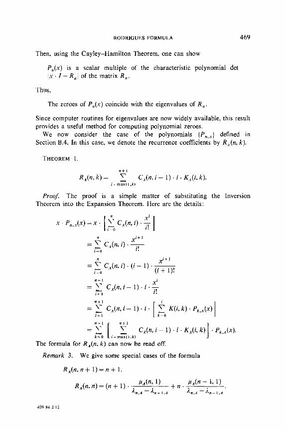
Then. using the Cayley-Hamilton Theorem, one can show

P,(X) is a scalar multiple of the characteristic polynomial det 1-x. I - R,I of the matrix R,.

Thus,

The zeroes of P,(X) coincide with the eigenvalues of R,.

Since computer routines for eigenvalues are now widely available, this result provides a useful method for computing polynomial zeroes.

We now consider the case of the polynomials {Pn.,l} defined in Section B.4. In this case, we denote the recurrence coefficients by R,(n, k).

THEOREM 1.

tlfl R,(n, k) = 1 C,(n, i - 1) . i. K,4(i, k).

i=maxfl.k)

Proof. The proof is a simple matter of substituting the Inversion Theorem into the Expansion Theorem. Here are the details:

x . P,,,(-U) =X - [t C,4(n, i) . G ] i=O

ii- 1 = t C,4(n, i) . +

i=O

= G C,4(n, i) . (i + 1) . & ,G ll+, i

= E C,(n,i-1)-i.+ i=l

II+1

= x C,4(n,i- l).i. $ K(i,k). Pk,A(x) i=l [ k=O 1 ?I+1 n+1 ZZ -7‘ [ r k%C, -

C,(n, i - 1) . i . K,(i, k) . Pk,A(.~). i=max(l.k) I

The formula for R,4(n, k) can now be read off.

Remark 3. We give some special cases of the formula

R,4(n, n + 1) = n + 1.

P,h 1) WwQ=(n+lb~ -A

+n. P.&- 131) II,.4 n+l.A A n , A -1 . n- 1.

JO9~W2 I2

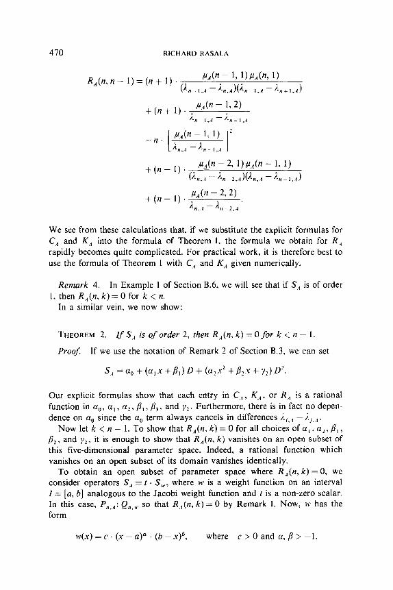
410 RICHARD RASALA

PAN - 4 l)PAh 1) R,4(nyn- 1)=(n+1)~(~.-,,.4-~n.A)(~n~I..4-~n+l..o

P,4@ - 17 2) +(n+u) -/z

n-1.,4 n+ I..4

-n. [ P,@- 1) 1, 2 1 Il.-l --A “-I./( I

- - + (n - l) * iu,(n 2, l)iu,(n 1, 1)

%I.., - L2,&,.4 -4-I.,)

+(n- 1)’ lu,(n - 2, 2) ~

Il..4 -A . n - 2.4

We see from these calculations that, if we substitute the explicit formulas for C,, and K, into the formula of Theorem 1, the formula we obtain for R, rapidly becomes quite complicated. For practical work, it is therefore best to use the formula of Theorem 1 with C,d and K,4 given numerically.

Remark 4. In Example 1 of Section B.6. we will see that if S,d is of order 1. then R,d(n, k)= 0 for k < n.

In a similar vein, we now show:

THEOREM 2. I” .S4 is of order 2, then R,4(n, k) = 0 for k i n - 1.

Proof. If we use the notation of Remark 2 of Section B.3, we can set

S,4=a,+((1,x+p,)D+(az”Z+Pz”+Yz)D?.

Our explicit formulas show that each entry in C,d, K,, or R,4 is a rational function in uO, c(, , CQ, /I,, p3, and yz . Furthermore, there is in fact no dependence on a,, since the a, term always cancels in differences Ai. 1 - Ai..,, .

Nowletk<n-l.ToshowthatR,(n,k)=Oforallchoicesofu,.a~,~,, /3*, and yZ, it is enough to show that R,q(n, k) vanishes on an open subset of this five-dimensional parameter space. Indeed, a rational function which vanishes on an open subset of its domain vanishes identically.

To obtain an open subset of parameter space where R,4(n, k) = 0, we consider operators S, = t . S,, where w is a weight function on an interval I = [a, 61 analogous to the Jacobi weight function and t is a non-zero scalar. In this case, P,,,.,,: Q,,, so that R,,(n, k) = 0 by Remark 1. Now, rt’ has the form

w(x) = c . (x - up . (b - x)“, where c>Oanda,p>-1.


Then,

S., = r . S,,. = t[(x - u)(b - x) D2 + (ub + flu - (a + /3 + 2) x) D]

=[-t(u+/?+2)x+t(ub+~u)]~D + [-tx’ + t(a + b) x - tub] . D’.

We can equate the two formulas for S, and express a,, az, /?, , /?!. yZ in terms of a. b. cf. B, f:

cf, = -t(a + p + 2),

a?=-I,

P, = t(ub + Pu),

p2 = f(U + b),

)I? = -tab.

A simple calculation shows that the Jacobian of this transformation is 1 t IJ . 1 b - a(‘. Since the domain of the map is the open set

((a,b,a,p,t):u<b;a,p>-l;t#O},

the image of the map contains an open set in (a,. a?, /?,,p2. yZ) space and we are done.

Remark 5. In thinking about possible generalizations of Theorem 2. we were led to make the following conjecture:

If S, is of order m, then R4(nr k) = 0 for k < n - m.

This conjecture is, however, false for m = 3 as we will see by example in the next section.

B.6. Examples

We will give an assortment of special examples of the theory of the previous sections. It will be useful to note that:

LEMMA 1. If A is regular. then P,q,4 is characterized by:

(1) PK, is a polynomial eigenfunction of S, of degree n. (2) The leading coeficient of P,.,4 is l/n!

Also. for convenience, we will assume A,(x) = 0, that is, that S,A has no constant term.

472 RICHARD RASALA

EXAMPLE 1. Operators of order 1. Let S-, = (ax + 6) D. Then by direct inspection one can see that the polynomials (ax + b)” are eigenfunctions of S. Then by Lemma 1 we see that

p,,. ,j (x) = $ . (x + b/a)“.

The recurrence relations therefore take the form

-y . k..4w = c-y + b/4 . P,..~(-Y) - (b/a) . P,,.,(-~) =(n+ l).P,+,,, C-v) - (b/a) . p,,. J-Y).

This calculation verifies Remark 4 of Section B.5.

EXAMPLE 2. Hermite operators. We see from Section A. 1 of Part A that the Hermite polynomials are eigenfunctions of the operator

S=D2f(-2X)D.

It will be convenient to consider a slightly more general family of operators. namely,

S, = D’ + (ax) D.

Throughout, we will use the parameter u as a subscript in place of the usual A which stands for the polynomial sequence

(0, ax, 1, 0, 0 ,.... ).

We compute the expansion and inversion coefficients for P,,., . We first need the eigenvalues /I,,, and the functions ,u,(s, m):

A,,., = an,

&(S, m) = 1 if m=2

=o otherwise.

In the Expansion and Inversion Theorems, we must sum over certain sequences of indices m, ,..., m,. In view of the formula for ,ua, the only non- zero contributions occur when m, = ... = m, = 2. We therefore obtain:

(1) If II - i is odd, then C,(n, i) = 0.

(2) If n - i = 2r, then


(3) If j - k is odd, then K,(j, k) = 0.

(4) If j - k = 2r, then

r-1

4Aj3 k) = n 1 1

q=. (ak - a(k + 2q + 2)) = (-2a)’ . r! *

We observe immediately:

Fact 1. K,(n, i) = Ca(nr i), that is, the inversion coefficients for P,., are the expansion coefficients for P,,,-,.

Fact 2. C,(n, i) depends only on n - i and K,(j, k) depends only on j - k.

The explicit formula for P,.,(x) is

pn’a(x) = ,,~,, (2a)’ . r! . (n - 2r)! ’

The standard Hermite polynomials H,(x) have leading coefficient 2” in degree ?r and correspond to the parameter a = -2. Thus,

H,(x) = 2” * n! . P”*-z(x) - 2r

=n! [ ,,L, Pa)’ . x” 1 r! * - (n 2r)! *

= n. 1 [ 2 (-1)‘. w-2r 0<r<ni2 r! * (n 2r)! - 1 .

EXAMPLE 3. Laguerre operators. From Section A.1 of Part A, the Laguerre polynomials Lip’ are eigenfunctions of the operator

S=x.D2+(a+ l-x).0

Again. it will be convenient to consider a more general family of operators, namely,

S,., =x . D’ + (ax + b) . D.

In this case, we will use the parameters a, b as subscripts. We now compute the expansion and inversion coefficients for Pn,a,b. We first give A,,,.* and &.b(S, ml:

2. n.a.b = na,

,q& m) = b + s if m=l

= 0 otherwise.

474 RICHARD RASALA

In this case, the summation indices m, ,.... m, of the Expansion and Inversion Theorems lead to non-zero terms only when m, = ... = m, = 1. We therefore obtain

i-k-l ~d..k k) = r 1 (b+k+q) (b +j _ l)(i-rl

y=o (ok-a(k+q+ I))= (-a)j-“. (j-k)!’

We observe:

Fact 1. K03J~l, i) = C,+,(rz. i). Thus, the inversion coefficients for P,r,o,h are the expansion coefficients for P,,,- o.h.

Fact 2. K,,,jn, i) = (-I)“-’ . Cl,.h(~z. i).

To interpret Fact 2. consider the polynomials

L rr.n&) = t-1 )” . P,r.d-~).

Then, for Ln,a.h. we have:

The II, i expansion coefficient is (-1)” . C,,,(n. i).

The j, k inversion coefficient is (-I )’ K,,,h( j, k).

We can read Fact 2 as

(-l)i . Koeb(n, i) = f-1)” . Co.Jn, i).

In other words:

Fact 3. For the polynomials L,r.u.h, the matrices of expansion and inversion coefficients coincide.

It is interesting that the polynomials Lnqa,b reduce precisely to the classical Laguerre polynomials upon specializing a, 6. Indeed:

Fact 4. L:‘(x) = L,, _ I.= + ,(.r).

To see this, note that a = - 1 b = a + 1 produces the differential equation for L:‘(x) and that both polynomials have the same leading coefficient, namely. (-l)“/n!. We conclude this discussion by giving the explicit formula for Lyyx):

L;‘(x) = L& - I,a+l(x) = C-1)” . pn.-l.n+l(X)

= <- t-1)' . (' + a)'"-" . vxi.

,ro i! . (n - i)!


Remark 1. A digression on umbra1 calculus. Our results on the Hermite and Laguerre polynomials fit into a more general pattern of results which are found by Rota ef al. [8] using umbra1 calculus. We will make some brief comments on how the two methods are related.

In our theory. the natural basis of polynomial space appears to be the polynomials Y/n!. Therefore, we will use this basis to describe operators on P. Let

P = (P,(x), P,(x) . . . . . P,(x) . ...)

denote a sequence of polynomials. Then we can define an operator CJ,: P + P uniquely by the condition

U&“/n!) = P,(x).

To reinterpret Examples 2 and 3, we introduce the sequences

P[al = (PO,&), P,.,(x) . . . . . P,.,(x! ,... ).

Lb, bl = (-&J-Y), ~,,n.h(+~)~.... L.,.,(x) . . . . ).

Then Example 2 says that UP,-a, is inverse to Up,a, and Example 3 says that u I ,(I b, is its own inverse.

A’ more straightforward way to define operators on P would be to associate to a polynomial sequence

Q = (Q&h Q,(-XL..., Q,(x)+..)

the operator C’o: P --* P defined by

V&“) = Q,(x).

If, for the sequence P defined earlier. we set

P* = (O! ’ P&Y), l! . P,(x) ,..., n! . P,(x) ,,.. ),

then we have

It is therefore easy to translate results between U’s and Vs. In the work of Rota et al. IS], an umbra1 operator in an operator Va such

that the following extra condition on Q holds:

Q,G +Y) = & c 1 ; . Q,(x). Qn-d~).

476 RICHARD RASALA

Note that if Q = P*, then the above condition translates to

P,(x + y) = -6 P&Y) . P,-&J). k=O

The key to the Rota theory is that composition of umbra1 operators is isomorphic to composition of formal power series. Therefore, inversion results for polynomial sequences can be obtained from inversion results for power series in those cases when the inverse of the associated power series can be found. Some additional nice results about Hermite and Laguerre polynomials are obtained using these ideas.

In contrast, our methods apply in principle to any polynomial sequence. What we must do is express the sequence as eigenfunctions of a regular polynomial differential operator. It is to be expected that our inversion formulas will, at first, be more complicated. It is more amazing that it is possible to write down inversion formulas at all.

We conclude this digression with two minor notes.

Note 1. If f is a polynomial and Q is a polynomial sequence. then the umbra1 compositionf(Q) defined by Rota is just V,(f).

Note 2. We have seen that UL,o.bl = VLra,b,, is its own inverse. This is exactly the result in Rota since he works with the operators Va and since the polynomials he denotes by Lip’ differ from the usual Laguerre polynomials by the factor n!.

Remark 2. Comments on the Hermite and Laguerre situations. The features which make possible the simple inversion results in the Hermite and Laguerre situations boil down to two conditions:

1: L.4 is linear in n. Equivalently, a,,, # 0 but a,,., = 0 for all m > 2. II: There exists M > 1 such that ,u~(s, m) is identically zero if m > 1

and m#M.

By itself, condition I implies a simplification of the denominators in the expansion and inversion formulas, namely:

LEMMA 1. Assume condition I and set a, .. = a. Let

Then

n-i=m, fem. +mrr t,=i+ x mp. PCY

r-1

r-1 L\ (liqA - Atq+,J = (-Jr . [ fj trnl + ... + mq)l .


By itself, condition II implies that there is at most one summand in the expansion and inversion formulas. More precisely:

LEMMA 2. Assume condition-II. Then:

(I) If M does nor dioide n - i, then C.,(n, i) = K,,,(n, i) = 0. (2) Assume M divides n - i. say, n - i = M . r. Then.

When both conditions I and II hold. we have the results of Lemma 3:

LEMMA 3. Assume conditions I and II. Set a, .0 = a and let n - i = M . r. Then.

C.&h i) = [

r-1 rl p.4(i + Mq, M) [ (aMY . r! 1,

9=0 Ii [ I-- I

K,4(n, i) = rI ,u,(i + Mq, M) [(-aM)’ . r!]. 4 =o Ii

In particular, K,4(n, i) = (-1)’ . C,(n, i). ’ Now, assuming conditions I and II, let A* denote the polynomial sequence

obtained from A by changing a to -a. Set:

Then:

P = (..., P,., ,... ),

P* = (..., P,,.,* )... ).

THEOREM. Assume conditions I and II. Then Up. is the inverse to CT,.

Question. Is it possible to define an involution A -+ A* on the set of regular polynomial sequences such that 17,. is inverse to II, ?

EXAMPLE 4. Jacobi and Gegenbauer polynomials. The Jacobi polynomials Pjp;+O) are the eigenfunctions of the operator

S = (1 - x’) . D’ + [/? - a - (a + ,8 + 2) x] . D.

For this operator, the non-trivial polynomials A,(x) are

A,(x) = 1 -x2, A,(x)=p-a-(a+/3+2)x.

478 RICHARD RASALA

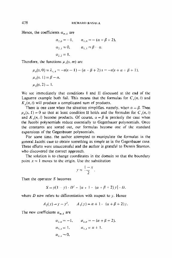
Hence, the coeffkients c(,,~ are

a 2.0 = -1. u,~,=-(U+p+2).

a -0. ?.I - u,,, =/3-u.

cl - 1, 2.z -

Therefore, the functions p.,(s, m) are

lu.&. 0) = 4., = --s(s- I)-(u+p+2)s=-s(s+cf+/3+ l),

iul(S. l)=B-a,

p,(s, 2) = 1.

We see immediately that conditions I and II discussed at the end of the Laguerre example both fail. This means that the formulas for C.,(n, i) and K,(n, i) will produce a complicated sum of products.

There is one case when the situation simplifies. namely, when a = /3. Then pu,(s, 1) = 0 so that at least condition II holds and the formulas for C,(n, i) and K4(nr i) become products. Of course, u =/I is precisely the case when the Jacobi polynomials reduce essentially to Gegenbauer polynomials. Once the constants are sorted out, our formulas become one of the standard expansions of the Gegenbauer polynomials.

For some time, the author attempted to manipulate the formulas in the general Jacobi case to obtain something as simple as in the Gegenbauer case. These efforts were unsuccessful and the author is grateful to Dennis Stanton. who discovered the correct approach.

The solution is to change coordinates in the domain so that the boundary point x = 1 moves to the origin. Use the substitution

1 --.Y J’=-.

2

Then the operator S becomes

s=J’(1-J’)~DL+lu+1-(u+/3+2)J1].D.

where D now refers to differentiation with respect to J+. Hence

z‘&(?‘)=J’-J”. A,(4’)=u+ l-(U+/!l+2)J’.

The new coefficients um,k are

U 2.0 = -1, u,*“=-(u+p+2).

a - 1, 2.1 - U ,., =a+ 1.

U - 0, 2.2 -


The new functions ,~,~(s. m) are

Pu,(S. 0) = A,..4 = -s(s- l)-((u+p+2)s=-s(s+a+p+ l).,

p,(s. l)=s+a+ 1.

,&(S, 2) = 0.

The eigenvalues A,,,4 are of course unchanged by the transformation. In contrast. the higher ,u, functions have changed and now condition II is satisfied. Hence the expansion and inversion coefftcients will be given by product formulas. Let us sketch the details. First, by a direct computation, we have

A,,.4 - A(,., = -(s - r)(s + t + a + p + 1).

Next. we apply Lemma 2. noting that 121 = 1 and r = II - i:

n-i-l

c,4(tz. i)= 1 [ (i+q+a+ 1)

y-,, -(n-(i+qjj(n+(i+qj+a+p+ 1) n- I

=(-I)“-’ n @?+a+ 1) y=i (tZ-qq)(tZ+q+a+/3+ 1)

= (-1)“‘L (a+ I), (rt+u+P+ ‘)i (17 -i)! (a + l)i (tz + a + /3 + l), ’

Here we have used the ascending factorial notation:

(a),. = a(a + 1) . ‘. . . (a + li - 1).

Using the above formula for C,(n. i). we can express PF9”‘(?c) in terms of the variable ~3:

P;.“‘(x) = const . T7 C,<(n, i) . $ ir,

= const . \ - n, (-7); (n + a +P + l)iJ,i

- ipo i! (U+l)i ’

Finally. the formula for K,4(n, i) can be computed in the same way as the one for C,,(n. ij, so we simply state the result:

K,(n, i) = 1 .(a+ 1); 1

n!~(a+l)i~(2i+a+~+l),~i’

The last term in the denominator does not break up as easily as the corresponding term in C,4(n, i).

480 RICHARD RASALA

EXAMPLE 5. A counterexample to a conjecture. At the end of Section B.5, the following conjecture on the recurrence coefficients was stated:

If S,, is of order m, then R,4(r~, k) = 0 for k < H - m. It is the purpose of this example to prove this conjecture false. The operator which yields the counterexample is

L&=(X’+ 1jD3+(.y)D2+(X+ IjO.

We will list enough data so that the reader can see that we have a counterexample to the conjecture.

( 1) The eigenvalues L,, A.

2 n,,4 = n + n(n - l)(n - 2).

n 0 1 2 3 4.

1 Il..4 0 1 2 9 28

(2) The functions ,u,~(s, m).

p.,(s, 1) =s + I, P.,(& 2) = 0, P.,(h 3) = 1, P.&, m) = 0 for m 24.

(3) The C, matrix.

1

1 1

1 2 1

621504 6156 3/l 1 33261373464 518113338 121494 4119 1

(4) The K, matrix.

1

-1 I

1 -2 1

-8j18 618 -3/l 1

501504 -321216 121182 -4119 1


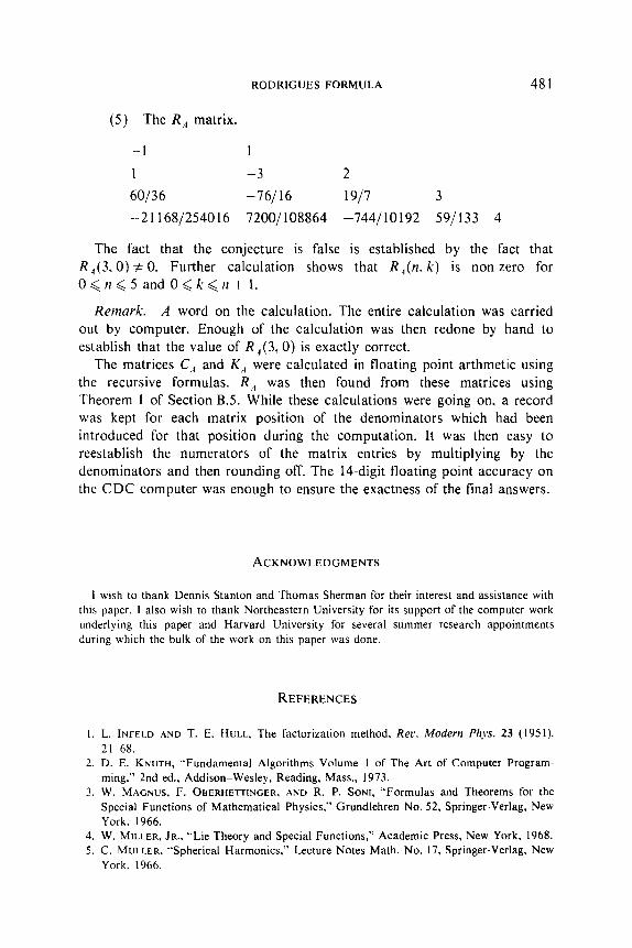
(5) The R,4 matrix.

-1 1

1 -3 2

60136 -76116 1917 3

-21168/254016 7200/108864 -744110192 591133 4

The fact that the conjecture is false is established by the fact that R ,(3.0) # 0. Further calculation shows that R ,(n. k) is non-zero for O<n<5 and O<k<rt+ 1.

Remark. A word on the calculation. The entire calculation was carried out by computer. Enough of the calculation was then redone by hand to establish that the value of R,(3, 0) is exactly correct.

The matrices C,d and K,, were calculated in floating point arthmetic using the recursive formulas. R., was then found from these matrices using Theorem 1 of Section B.5. While these calculations were going on, a record was kept for each matrix position of the denominators which had been introduced for that position during the computation. It was then easy to reestablish the numerators of the matrix entries by multiplying by the denominators and then rounding off. The 14.digit floating point accuracy on the CDC computer was enough to ensure the exactness of the final answers.

ACKNOWLEDGMENTS

I wish to thank Dennis Stanton and Thomas Sherman for their interest and assistance with this paper. I also wish to thank Northeastern University for its support of the computer work underlying this paper and Harvard University for several summer research appointments during which the bulk of the work on this paper was done.

REFERENCES

I. L. INFELD AND T. E. HULL. The factorization method. Rec. Modern Phys. 23 (1951). 2 l-68.

2. D. E. KNUTH, “Fundamental Algorithms Volume 1 of The Art of Computer Program- ming.” 2nd ed.. Addison-Wesley, Reading, Mass., 1973.

3. W. MAGNUS, F. OBERHETTINGER. AND R. P. SONI, “Formulas and Theorems for the Special Functions of Mathematical Physics.” Grundlehren No. 52, Springer-Verlag, New York, 1966.

4. W. MILLER. JR.. “Lie Theory and Special Functions,” Academic Press, New York, 1968. 5. C. MULLER. “Spherical Harmonics.” Lecture Notes Math. No. 17, Springer-Verlag, New

York. 1966.

482 RICHARD RASAL.4

6. R. MULLEN ANI) G.-C. ROTA, On the foundations of combinatorial theory. III. Theory of binomial enumeration. in “Graph Theory and Its Applications” (B. Harris, Ed.). pp. 167-2 13. Academic Press, New York. 1970.

7. A. ROBERT, “Systemes des Polynomes.” Queen’s Papers Pure Appl. hlath. No. 35. Queen’s Univ., Kingston, Ontario. Canada. 1973.

8. G.-C. RoT.~. “Finite Operator Calculus.” Academic Press. New York. 1975. 9. G. SZEGO. “Orthogonal Polynomials.” 4th ed., Amer. Math. Sot., Providence. R.I.. 1975.

IO. C. TRUESDELL. “An Essay Toward a Unified Theory of Special Functions.” Annals of Math. Studies No. 18. Princeton Univ. Press. Princeton. N.J.. 1948.

the rodrigues formula and polynomial differential operatorsthe rodrigues formula and polynomial...

Documents