The

Ha dbook

Brai T eory

al Networks

Michael A. Arbib

editor

I

First MIT Press paperback edition, 1998

© 1995 Massachusetts Institute of TechnologyAll rights reserved. No part of this book may be reproduced in any form by any electronic ormechanical means (including photocopying, recording, or information storage and retrieval)without permission in writing from the publisher.

This book was set in Times Roman by Asco Trade Typesetting Ltd., Hong Kong, and wasprinted and bound in the United States of America.

Library of Congress Cataloging-in-Publication Data

The handbook of brain theory and neural networks / Michael A. Arbib,editor.

p. cm.“A Bradford book.”Includes bibliographical references and index.ISBN 0-262-01148-4 (hc), 0-262-51102-9 (pb)1. Neural networks (Neurobiology)—Handbooks, manuals, etc.

2. Neural networks (Computer science)—Handbooks, manuals, etc.I. Arbib, Michael A.QP363.3.H36 1995612.8’2—dc2O 94—44408

CIP

804 Part III: Articles Reinforcement Learning 805

• Selective Bootstrap and AssociativeReward-Penalty Units

Blake, A., and Zisserman, A., 1987, Visual Reconstruction, Cambridge, Marroquin, J. L., and Ramirez, A., 1991, Stochastic cellular automa~ A stochastic learning automaton implements a common-sense which training examples it sees (see EXPLORATION IN ACTIVEMA: MIT Press. with invariant Gibbsian measures, IEEE Trans. Inform. Theory, 37: notion of reinforcement learning: if action a, is chosen on trial LEARNING).

Chellapa, R., and Jam, A., Eds., 1993, Markov Random Fields: Theory 541 551. and the critic’s feedback is “success,” then p,(t) is increasedand Practice, Boston: Academic Press. • Ortega, J. M., and Rheinholdt, W. C., 1970, Iterative Solution of Non.

Geman, S., and Geman, D., 1984, Stochastic relaxation, Gibbs distri- linear Equations in Several Variables, New York: Academic Press and the probabilities of the other actions are decreased; wherebutions and the Bayesian restoration of images, IEEE Trans. Pattern Poggio, T., and Girosi, F., 1990, Regularization algorithms for learn, as if the critic indicates “failure,” thenp,(t) is decreased and the Associative Reinforcement Learning RulesAnalysis Machine Intell., 6:721—741. ing that are equivalent to multilayer networks, Science, 247:978_992. probabilities of the other actions are appropriately adjusted. Several associative reinforcement learning rules for neuron-like

Grimson, W. E. L., 1982, A computer implementation of a theory of Poggio, T., Yang, W., and Torre, V., 1989, Optical flow: Compu~, Many methods for adjusting action probabilities have been units have been studied. Consider a neuron-like unit receivingstereo vision, Philos. Trans. R. Soc. Lond. B Biol. Sci., 298. tional properties and networks, biological and analog, in The Corn. studied, and numerous theorems have been proven about how a stimulus pattern as input in addition to the critic’s reinforce

Kemeny, J. G., and Snell, J. L., 1960, Finite Markov Chains and Their puting Neuron (R. Durbin, C. Miall, and G. Mitchison, Eds.), Read- they perform. ment signal. Let x(t), w(t), a(t), and r(t), respectively, denoteApplications, New York: Van Nostrand. ing, MA: Addison-Wesley. One can generalize this nonassociative problem to illustrate the stimulus vector, weight vector, action, and value of the

Marroquin, J. L., 1992, Random measure fields and the integration of Pomerleau, D. A., 1991, Efficient training of artificial neural networks an associative reinforcement learning problem. Suppose that reinforcement signal at time 1. Let s(t) denote the weighted sumvisual information, IEEE Trans. Syst. Man Cybern., 22:705 716. for autonomous navigation, Neural Computat., 3:88—97.

Marroquin, J. L., Mitter, S., and Poggio, T., 1987, Probabilistic solu- Tikhonov, A. N., and Arsenin, V. Y., 1977, Solutions ofIll-Posed Pro!,.. on trial t the learning system senses stimulus pattern x(t) and of the stimulus components at time I:tion of ill-posed problems in computational vision, J. Am. Statist. lems, Washington, DC: Winston and Sons. selects an action a(l) = a through a process that can depend onAssoc., 82:76—89. x(t). After this action is executed, the critic signals success with s(t) = ~ w,(t)x(t)

probability d1(x(t)) and failure with probability 1 — d~(x(t)).The objective of learning is to maximize success probability, where w1(t) and x,(t), respectively, are the ith components ofachieved when on each trial t the learning system executes the weight and stimulus vectors.the action a(t) = a~, where aj is the action such that d~(x(t))max{d,(x(t))Ii = 1,... ,m}. Unlike supervised learning, exam

Reinforcement Learning ples of optimal actions are not provided during training; they Associative Search Unithave to be discovered through exploration by the learning

Andrew G. Bar to sytem. Learning tasks like this are related to instrumental, or One simple associative reinforcement learning rule is an extension of the Hebbian correlation learning rule. This rule, calledcued operant, tasks used by animal learning theorists, and the the associative search rule, was motivated by Klopf’s (1982)

stimulus patterns correspond to discriminative stimuli.Introduction reinforcement Critic Following are key observations about both nonassociative theory of the self-interested neuron. To exhibit variety in itsbehavior, the unit’s output is a random variable depending onand associative reinforcement learning: the activation level:

in experimental psychology, where it refers to the occurrence ofThe term reinforcement comes from studies of animal learning signal example, if the critic in the preceding example evaluated a(t) ~0 with probability 1 — p(t)

1. Uncertainty plays a key role in reinforcement learning. For Ii with probability pQ)an event, in the proper relation to a response, that tends to stimulus { — — .01..] Learning I actions 1~J l~OC~~(1)increase the probability that the response will occur again in patterns — .~..j system I

the same situation. Although not used by psychologists, the I I actions deterministically (i.e., d, = I or 0 for each i), thenterm reinforcement learning has been widely adopted by the- I process -‘ the problem would be a much simpler optimization prob- where p(t), which must be between 0 and 1, is an increasing

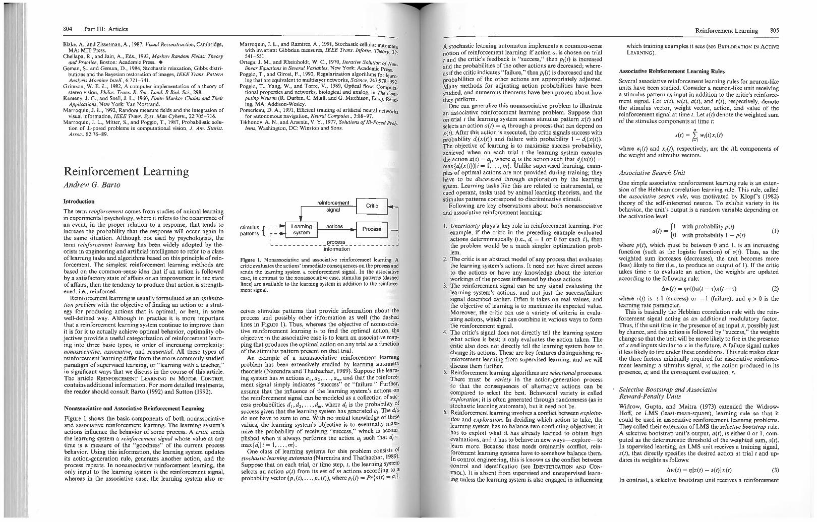
informationorists in engineering and artificial intelligence to refer to a class lem. function (such as the logistic function) of s(t). Thus, as theof learning tasks and algorithms based on this principle of rein- Figure 1. Nonassociative and associative reinforcement learning. A 2. The critic is an abstract model of any process that evaluates weighted sum increases (decreases), the unit becomes moreforcement. The simplest reinforcement learning methods are critic evaluates the actions’ immediate consequences on the process and the learning system’s actions. It need not have direct access (less) likely to fire (i.e., to produce an output of 1). If the criticbased on the common-sense idea that if an action is followed sends the learning system a reinforcement signal. In the associative to the actions or have any knowledge about the interior takes time z to evaluate an action, the weights are updatedby a satisfactory state of affairs or an improvement in the state case, in contrast to the nonassociative case, stimulus patterns (dashed workings of the process influenced by those actions. according to the following rule:of affairs, then the tendency to produce that action is strength- lines) are available to the learning system in addition to the reinforce- 3. The reinforcement signal can be any signal evaluating the t~w(t) = ~r(t)a(t — t)x(t — r) (2)ened, i.e., reinforced. ment signal. learning system’s actions, and not just the success/failure

Reinforcement learning is usually formulated as an optimiza- signal described earlier. Often it takes on real values, and where r(t) is + 1 (success) or — 1 (failure), and ~ > 0 is thelion problem with the objective of finding an action or a strat- the objective of learning is to maximize its expected value, learning rate parameter.egy for producing actions that is optimal, or best, in some ceives stimulus patterns that provide information about the Moreover, the critic can use a variety of criteria in evalu- This is basically the Hebbian correlation rule with the rein-well-defined way. Although in practice it is more important process and possibly other information as well (the dashed ating actions, which it can combine in various ways to form forcement signal acting as an additional modulatory factor.that a reinforcement learning system continue to improve than lines in Figure 1). Thus, whereas the objective of nonassocia- the reinforcement signal. Thus, if the unit fires in the presence of an input x, possibly justit is for it to actually achieve optimal behavior, optimality ob- tive reinforcement learning is to find the optimal action, the 4. The critic’s signal does not directly tell the learning system by chance, and this action is followed by “success,” the weightsjectives provide a useful categorization of reinforcement learn- objective in the associative case is to learn an associative map- what action is best; it only evaluates the action taken. The change so that the unit will be more likely to fire in the presenceing into three basic types, in order of increasing complexity: ping that produces the optimal action on any trial as a function critic also does not directly tell the learning system how to of x and inputs similar to x in the future. A failure signal makesnonassociative, associative, and sequential. All these types of of the stimulus pattern present on that trial, change its actions. These are key features distinguishing re- it less likely to fire under these conditions. This rule makes clearreinforcement learning differ from the more commonly studied An example of a nonassociative reinforcement learning inforcement learning from supervised learning, and we will the three factors minimally required for associative reinforce-paradigm of supervised learning, or “learning with a teacher,” problem has been extensively studied by learning automata discuss them further. ment learning: a stimulus signal, x; the action produced in itsin significant ways that we discuss in the course of this article, theorists (Narendra and Thathachar, 1989). Suppose the learn- 5. Reinforcement learning algorithms are selectional processes. presence, a; and the consequent evaluation, r.The article REINFORCEMENT LEARNING IN MOTOR CONTROL ing system has m actions a1, a2,. . . , a,,,, and that the reinforce- There must be variety in the action-generation processcontains additional information. For more detailed treatments, ment signal simply indicates “success” or “failure.” Further, so that the consequences of alternative actions can bethe reader should consult Barto (1992) and Sutton (1992). assume that the influence of the learning system’s actions on compared to select the best. Behavioral variety is called

the reinforcement signal can be modeled as a collection of sue- exploration; it is often generated through randomness (as in

Nonassociative and Associative Reinforcement Learning cess probabilities d1 , d2 dm, where d, is the probability of stochastic learning automata), but it need not be. Widrow, Gupta, and Maitra (1973) extended the Widrowsuccess given that the learning system has generated a1. The d1’s 6. Reinforcement learning involves a conflict between exploita- Hoff, or LMS (least-mean-square), learning rule so that itFigure 1 shows the basic components of both nonassociative do not have to sum to one. With no initial knowledge of these lion and exploration. In deciding which action to take, the could be used in associative reinforcement learning problems.and associative reinforcement learning. The learning system’s values, the learning system’s objective is to eventually maxi- learning system has to balance two conflicting objectives: it They called their extension of LMS the selective bootstrap rule.actions influence the behavior of some process. A critic sends mize the probability of receiving “success,” which is accom’ has to exploit what it has already learned to obtain high A selective bootstrap unit’s output, a(t), is either 0 or 1, corn-the learning system a reinforcement signal whose value at any plished when it always performs the action a~ such that ‘~ evaluations, and it has to behave in new ways—explore—to puted as the deterministic threshold of the weighted sum, s(t).time is a measure of the “goodness” of the current process max{d, I i = 1 m}. learn more. Because these needs ordinarily conflict, rein- In supervised learning, an LMS unit receives a training signal,behavior. Using this information, the learning system updates One class of learning systems for this problem conSistS of forcement learning systems have to somehow balance them. z(t), that directly specifies the desired action at trial t and up-its action-generation rule, generates another action, and the stochastic learning automata (Narendra and Thathachar, 1989). In control engineering, this is known as the conflict between dates its weights as follows:process repeats. In nonassociative reinforcement learning, the Suppose that on each trial, or time step, t, the learning system control and identification (see IDENTIFICATION AND CON

E~w(t) = ~[z(t) — s(t)]x(t) (3)only input to the learning system is the reinforcement signal, selects an action a(t) from its set of m actions according to a TROL) It is absent from supervised and unsupervised learn-whereas in the associative case, the learning system also re- probability vector (Pi (t) pm(t)), wherep1(t) = Pr{a(t) = a1}. ing unless the learning system is also engaged in influencing In contrast, a selective bootstrap unit receives a reinforcement

806 Part III: Articles Reinforcement Learning 807

signal, r(t), and updates its weights according to this rule:

Aw(t) — Ji[a(t) — sQ)]x(t) if r(t) = success— )~[l — a(t) — s(t)]x(t) if r(t) = failure

where it is understood that r(t) evaluates a(t). Thus, if a(t)produces “success,” the LMS rule is applied with a(t) playingthe role of the desired action. Widrow et al. (1973) called thispositive bootstrap adaptation: weights are updated as if the output actually produced was in fact the desired action. On theother hand, if a(t) leads to “failure,” the desired action is

— a(t), i.e., the action that was not produced. This is negativebootstrap adaptation. The reinforcement signal switches theunit between positive and negative bootstrap adaptation, motivating the term selective bootstrap adaptation.

A closely related unit is the associative reward-penalty (AR_p)unit of Barto and Anandan (1985). It differs from the selectivebootstrap algorithm in two ways. First, the unit’s output is arandom variable like that of the associative search unit (Equation 1). Second, its weight-update rule is an asymmetric versionof the selective bootstrap rule:

~ — $n[a(t) — sQ)]x(t) if r(t) = successW — 1A,,[l — a(t) — s(t)]x(t) if r(t) = failure

where 0 <A ≤ 1 and ~ > 0. This rule’s asymmetry is importantbecause its asymptotic performance improves as A approacheszero, but A = 0 is, in general, not optimal.

We can see from the selective bootstrap and AR_p units thata reinforcement signal is less informative than a signal specifying a desired action. It is also less informative than the errorz(t) — a(t) used by the LMS rule. Because this error is a signedquantity, it tells the unit how, i.e., in what direction, it shouldchange its action. A reinforcement signal—by itself—does notconvey this information. If the learner has only two actions, itis easy to deduce, or estimate, the desired action from the reinforcement signal and the actual action. However, if there aremore than two actions, the situation is more difficult becausethe reinforcement signal does not provide information aboutactions that were not taken. One way a neuron-like unit withmore than two actions can perform associative reinforcementlearning is illustrated by the Stochastic Real- Valued (SRV) unitof Gullapalli described in REINFORCEMENT LEARNING IN MOTORCONTROL.

Weight Perturbation

For the units described in the preceding section (except theselective bootstrap unit), behavioral variability is achieved byincluding random variation in the unit’s output. Another approach is to randomly vary the weights. Following Aispector etal. (1993), let ~w be a vector of small perturbations, one foreach weight, which are independently selected from some probability distribution. Letting 8’ denote the function evaluatingthe system’s behavior, the weights are updated as follows:

E8’(w + ow) —

= —‘11[ Ow

where ~ > 0 is a learning rate parameter. This is a gradientdescent learning rule that changes weights according to an estimate of the gradient of 8’ with respect to the weights. Aispectoret al. (1993) say that the method measures the gradient insteadof calculating it as the LMS and error backpropagation algorithms do. This approach has been proposed by several researchers for updating the weights of a unit, or of a network,during supervised learning, where 8’ gives the error over thetraining examples. However, 8’ can be any function evaluating

the unit’s behavior, including a reinforcement function (inwhich case, the sign of the learning rule would be changed tomake it a gradient ascent rule).

Reinforcement Learning Networks

Networks of AR_p units have been used successfully in bothsupervised and associative reinforcement learning tasks (Barto,1985; Barto and Jordan, 1987), although only with feedforwardconnection patterns. For supervised learning, the output unitslearn just as they do in error backpropagtion, but the hiddenunits learn according to the AR_P rule. The reinforcement signal, which is defined to increase as the output error decreases,is simply broadcast to all the hidden units, which learn simultaneously. If the network as a whole faces an associative reinforcement learning task, all the units are AR_p units, to whichthe reinforcement signal is uniformly broadcast (Barto, 1985).Another way to use reinforcement learning units in networksis to use them only as output units, with hidden units beingtrained via backpropagation. Weight changes of the outputunits determine the quantities that are backpropagated. An example is provided by a network for robot peg-in-hole insertiondescribed in REINFORCEMENT LEARNING IN MOTOR CONTROL.

The error backpropagation algorithm can be used in anotherway in associative reinforcement learning problems. It is possible to train a multilayer network to form a model of the processby which the critic evaluates actions. After this model is trainedsufficiently, it is possible to estimate the gradient of the reinforcement signal with respect to each component of the actionvector by analytically differentiating the model’s output withrespect to its action inputs (which can be done efficiently bybackpropagation). This gradient estimate is then used toupdate the parameters of an action-generation component.Jordan and Jacobs (1990) illustrate this approach.

The weight perturbation approach carries over directly tonetworks by simply letting w in Equation 4 be the vector consisting all the network’s weights. A number of researchers haveachieved success using this approach in supervised learningproblems. In these cases, one can think of each weight as facinga reinforcement learning task (which is in fact nonassociative),even though the network as a whole faces a supervised learningtask. An advantage of this approach is that it applies to networks with arbitrary connection patterns, not just to feedforward networks.

It should be clear from this discussion of reinforcementlearning networks that there are many different approaches tosolving reinforcement learning problems. Furthermore, although reinforcement learning tasks can be clearly distinguished from supervised and unsupervised learning tasks, it ismore difficult to precisely define a class of reinforcement learning algorithms.

Sequential Reinforcement Learning

Sequential reinforcement requires improving the long-term(4) consequences of an action, or of a strategy for performing

actions, in addition to short-term consequences. In theseproblems, it can make sense to forgo short-term performancein order to achieve better performance over the long term.Tasks having these properties are examples of optimal controlproblems, sometimes called sequential decision problems whenformulated in discrete time (see ADAPTIVE CONTROL: NEURALNETWORK APPLICATIONS).

Figure 1, which shows the components of an associative reinforcement learning system, also applies to sequential reinforcement learning, where the box labeled “Process” is a system

being controlled. A sequential reinforcement learning systemtries to influence the behavior of the process in order to maximize a measure of the total amount of reinforcement that willbe received over time. In the simplest case, this measure is thesum of the future reinforcement values, and the objective is tolearn an associative mapping that at each time step t selects,as a function of the stimulus pattern x(t), an action a(t) thatmaximizes

k~O r(t + k)

where r(t + k) is the reinforcement signal at step t + k. Such anassociative mapping is called a policy.

Because this sum might be infinite in some problems, andbecause the learning system usually has control only over itsexpected value, researchers often consider the following expected discounted sum instead:

E{r(t) + yr(t + 1) + y2r(t + 2) + . . . } E{~ y~(t + k)}

(5)

where E is the expectation over all possible future behaviorpatterns of the process. The discount factor y determines thepresent value of future reinforcement: a reinforcement valuereceived k time steps in the future is worth y” times what itwould be worth if it were received now. If 0 ≤ y < 1, this infinite discounted sum is finite as long as the reinforcement valuesare bounded. If y = 0, the robot is “myopic” in being onlyconcerned with maximizing immediate reinforcement; this isthe associative reinforcement learning problem discussed earlier. As y approaches 1, the objective explicitly takes future reinforcement into account: the robot becomes more farsighted.

An important special case of this problem occurs when thereis no immediate reinforcement until a goal state is reached.This is a delayed reward problem in which the learning systemhas to learn how to make the process enter a goal state. Sometimes the objective is to make it enter a goal state as quickly aspossible. A key difficulty in these problems has been called thetemporal credit-assignment problem: When a goal state is finallyreached, which of the decisions made earlier deserve credit forthe resulting reinforcement? (See also REINFORCEMENT LEARNING IN MOTOR CONTROL.) A widely studied approach to thisproblem is to learn an internal evaluation function that is moreinformative than the evaluation function implemented by theexternal critic. An adaptive critic is a system that learns such aninternal evaluation function.

Samuel’s Checkers Player

Samuel’s (1959) checkers-playing program has been a majorinfluence on adaptive critic methods. The checkers player usesan evaluation function to assign a score to each board configuration; and the system makes the move expected to lead to theconfiguration with the highest score. Samuel used a method toimprove the evaluation function through a process that compared the score of the current board position with the score ofa board position likely to arise later in the game. As a result ofthis process of “backing up” board evaluations, the evaluationfunction improved in its ability to evaluate the long-term consequences of moves. If the evaluation function can be made toScore each board configuration according to its true promise ofeventually leading to a win, then the best strategy for playing isto myopically select each move so that the next board configuration is the most highly scored. If the evaluation function isOptimal in this sense, then it already takes into account all the

possible future courses of play. Methods such as Samuel’s thatattempt to adjust the evaluation function toward this idealoptimal evaluation function are of great utility.

Adaptive Critic Unit and Temporal Difference Methods

An adaptive critic unit is a neuron-like unit that implementsa method similar to Samuel’s. The unit is a neuron-like unitwhose output at time step t is P(t) = E~ w~(t)x1(t), so denotedbecause it is a prediction of the discounted sum of future reinforcement defined by Equation 5. The adaptive critic learningrule rests on noting that correct predictions must satisfy a consistency condition relating predictions at adjacent time steps.Suppose that the predictions at any two successive time steps,say steps t and t + 1, are correct. This assumption means that

P(t) = E{r(t) + yr(t + 1) + y2r(t + 2) + . . . }P(t + 1) = E{r(t + 1) + yr(t + 2) + y2r(t + 3) + . . . }

Now notice that we can rewrite P(t) as follows:

P(t) = E{r(t) + y[r(t + 1) + yr(t + 2) + . . .

But this is exactly the same as

P(t) = E{r(t)} + yP(t + 1)

An estimate of the error by which any two adjacent predictionsfail to satisfy this consistency condition is called the temporaldifference (TD) error (Sutton, 1988):

r(t) + ‘yP(t + 1) — P(t) (6)

where r(t) is used as an unbiased estimate of E{r(t)}. The termtemporal difference comes from the fact that this error essentially depends on the difference between the critic’s predictionsat successive time steps.

The adaptive critic unit adjusts its weights according to thefollowing learning rule:

Aw(t) = ~i[r(t) + yP(t + 1) — P(t)]x(t) (7)

A subtlety here is that P(t + 1) should be computed using theweight vector w(t), not w(t + 1). This rule changes the weightsto decrease the magnitude of the TD error. Note that if y = 0,it is equal to the LMS learning rule (Equation 3). By analogywith the LMS rule, we can think of r(t) + yP(t + 1) as theprediction target: it is the quantity that each P(t) should match.The adaptive critic is therefore trying to predict the next reinforcement, r(t), plus its own next (discounted) prediction,yP(t + 1). It is similar to Samuel’s learning method in adjustingweights to make current predictions closer to later predictions.

Although this method is very simple computationally, it actually converges to the correct predictions of the expected discounted sum of future reinforcement if these correct predictions can be computed by a linear unit. This finding is shownby Sutton (1988), who discusses a more general class of methods, called TD methods, that include Equation 7 as a specialcase. It is also possible to learn nonlinear predictions using, forexample, multilayer networks trained by back propagating theTD error. Using this approach, Tesauro (1992) produced asystem that learned how to play expert-level backgammon.

Actor-Critic Architectures

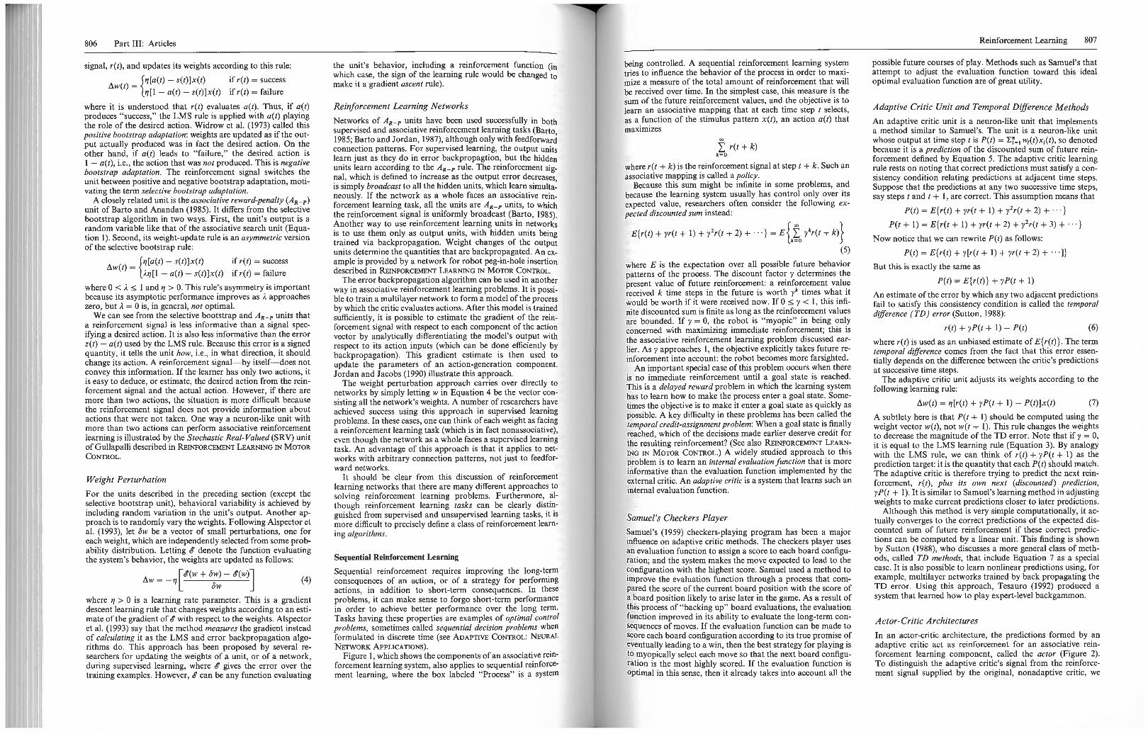
In an actor-critic architecture, the predictions formed by anadaptive critic act as reinforcement for an associative reinforcement learning component, called the actor (Figure 2).To distinguish the adaptive critic’s signal from the reinforcement signal supplied by the original, nonadaptive critic, we

808 Part III: Articles Reinforcement Learning in Motor Control 809

call it the internal reinforcement signal. The actor tries tomaximize the immediate internal reinforcement signal, whilethe adaptive critic tries to predict total future reinforcement.To the extent that the adaptive critic’s predictions of total future reinforcement are correct given the actor’s current policy,the actor actually learns to increase the total amount of futurereinforcement.

Barto, Sutton, and Anderson (1983) used this architecturefor learning to balance a simulated pole mounted on a cart.The actor had two actions: application of a force of a fixedmagnitude to the cart in the plus or minus directions. The nonadaptive critic only provided a signal of failure when the polefell past a certain angle or the cart hit the end of the track.The stimulus patterns were vectors representing the state ofthe cart-pole system. The actor was essentially an associativesearch unit as described above whose weights were modulatedby the internal reinforcement signal.

Q-Learning

Another approach to sequential reinforcement learning combines the actor and adaptive critic into a single component thatlearns separate predictions for each action. At each time stepthe action with the largest prediction is selected, except for anexploration factor that causes other actions to be selected occasionally. An algorithm for learning predictions of future reinforcement for each action, called the Q-learning algorithm, wasproposed by Watkins (1989), who proved that it converges tothe correct predictions under certain conditions. Although theQ-learning convergence theorem requires lookup-table storage(and therefore finite state and action sets), many researchershave heuristically adapted Q-learning to more general forms ofstorage, including multilayer neural networks trained by back-propagating the Q-learning error.

Dynamic Programming

Sequential reinforcement learning problems (in fact, all reinforcement learning problems) are examples of stochastic optimal control problems. Among the traditional methods forsolving these problems are dynamic programming (DP) algorithms. As applied to optimal control, DP consists of methodsfor successively approximating optimal evaluation functionsand optimal policies. Bertsekas (1987) provides a good treatment of these methods. A basic operation in all DP algorithmsis “backing up” evaluations in a manner similar to the operation used in Samuel’s method and in the adaptive critic.

Recent reinforcement learning theory exploits connectionswith DP algorithms while emphasizing important differences.Following is a summary of key observations:

1. Because conventional DP algorithms require multiple exhaustive “sweeps” of the process state set (or a discretizedapproximation of it), they are not practical for problemswith very large finite state sets or high-dimensional con-

Figure 2. Actor-critic architecture. An adaptive critic provides aninternal reinforcement signal to an actor which learns a policy forcontrolling the process.

tinuous state spaces. Sequential reinforcement learningalgorithms approximate DP algorithms in ways designed toreduce this computational complexity.

2. Instead of requiring exhaustive sweeps, sequential reinforcement learning algorithms operate on states as they occur inactual or simulated experiences in controlling the process. Itis appropriate to view them as Monte Carlo DP algorithms.

3. Whereas conventional DP algorithms require a completeand accurate model of the process to be controlled, sequential reinforcement learning algorithms do not require such amodel. Instead of computing the required quantities (suchas state evaluations) from a model, they estimate thesequantities from experience. However, reinforcement learning methods can also take advantage of models to improvetheir efficiency.

It is therefore accurate to view sequential reinforcement learning as a collection of heuristic methods providing computationally feasible approximations of DP solutions to stochasticoptimal control problems.

Discussion

The increasing interest in reinforcement learning is due to itsapplicability to learning by autonomous robotic agents. Although both supervised and unsupervised learning can playessential roles in reinforcement learning systems, these paradigms by themselves are not general enough for learning whileacting in a dynamic and uncertain environment. Among thetopics being addressed by current reinforcement learning research are these: extending the theory of sequential reinforcement learning to include generalizing function approximationmethods; understanding how exploratory behavior is best introduced and controlled; sequential reinforcement learningwhen the process state cannot be observed; how problem-specific knowledge can be effectively incorporated into reinforcement learning systems; the design of modular and hierarchical architectures; and the relationship to brain rewardmechanisms.

Road Map: Learning in Artificial Neural Networks, DeterministicBackground: 1.3. Dynamics and Adaptation in Neural NetworksRelated Reading: Planning, Connectionist; Problem Solving, Connec

tionist

References

Alspector, J., Meir, R., Yuhas, B., Jayakumar, A., and Lippe, D.,1993, A parallel gradient descent method for learning in analogVLSI neural networks, in Advances in Neural Information processingSystems 5 (S. J. Hanson, J. D. Cowan, and C. L. Giles, Eds.), SanMateo, CA: Morgan Kaufmann, pp. 836—844.

Barto, A. G., 1985, Learning by statistical cooperation of self-interested neuron-like computing elements, Hum. Neurobiol., 4:229—256.

Barto, A. G., 1992, Reinforcement learning and adaptive critic methods, in Handbook of Intelligent Control: Neural, Fuzzy, and Adaptive

Approaches (D. A. White and D. A. Sofge, Eds.), New York: VanNostrand Reinhold, pp. 469—491.

Barto, A. G., and Anandan, P., 1985, Pattern recognizing stochasticlearning automata, IEEE Trans. Syst. Man Cybern., 15:360 375.

Barto, A. G., and Jordan, M. I., 1987, Gradient following withoutback-propagation in layered networks, in Proceedings of the IEEEFirst Annual Conference on Neural Networks (M. Caudill and C.Butler, Eds.), San Diego: IEEE, pp. 11629 11636.

Barto, A. G., Sutton, R. S., and Anderson, C. W., 1983, Neuronlikeelements that can solve difficult learning control problems, IEEETrans. Syst. Man Cybern., 13:835—846. Reprinted in Neurocomputing: Foundations of Research (J. A. Anderson and E. Rosenfeld,Eds.), Cambridge, MA: MIT Press, 1988.

Bertsekas, D. P., 1987, Dynamic Programming: Deterministic and Stochastic Models, Englewood Cliffs, NJ: Prentice Hall. •

Jordan, M. 1., and Jacobs, R. A., 1990, Learning to control an unstablesystem with forward modeling, in Advances in Neural InformationProcessing Systems 2 (D. S. Touretzky, Ed.), San Mateo, CA: MorganKaufmann, pp. 324 331.

Jordan, M. I., and Rumelhart, D. E., 1992, Supervised learning with adistal teacher, Cognit. Sci., 16:307—354.

Andrew G. Barto

Introduction

How do we learn motor skills such as reaching, walking, swimming, or riding a bicycle? Although there is a large literature onmotor skill acquisition which is full of controversies (for a recent introduction to human motor control, see Rosenbaum,1991), there is general agreement that motor learning requiresthe learner, human or not, to receive response-produced feedback through various senses providing information about performance. Careful consideration of the nature of the feedbackused in learning is important for understanding the role ofreinforcement learning in motor control (see REINFORCEMENTLEARNING). One function of feedback is to guide the performance of movements. This is the kind of feedback with whichwe are familiar from control theory, where it is the basis ofservomechanisms, although its role in guiding animal movement is more complex. Another function of feedback is to provide information useful for improving subsequent movement.Feedback having this function has been called learning feedback. Note that this functional distinction between feedbackfor control and for learning does not mean that the signals orchannels serving these functions need to be different.

Learning Feedback

When motor skills are acquired without the help of an explicitteacher or trainer, learning feedback must consist of information automatically generated by the movement and its consequences on the environment. This has been called intrinsic feedback (Schmidt, 1982). The “feel” of a successfully completedmovement and the sight of a basketball going through thehoop are examples of intrinsic learning feedback. A teacher ortrainer can augment intrinsic feedback by providing extrinsicfeedback (Schmidt, 1982) consisting of extra information addedfor training purposes, such as a buzzer indicating that a movement was on target, a word of praise or encouragement, or anindication that a certain kind of error was made.

Klopf, A. H., 1982, The Hedonistic Neuron: A Theory of Memory,Learning, and Intelligence, Washington, DC: Hemisphere.

Narendra, K., and Thathachar, M. A. L., 1989, Learning Automata:An Introduction, Englewood Cliffs, NJ: Prentice Hall. •

Samuel, A. L., 1959, Some studies in machine learning using the gameof checkers, IBM J. Res. Develop., 3:210 229. Reprinted in Computers and Thought (E. A. Feigenbaum and J. Feldman, Eds.), NewYork: McGraw-Hill, 1963, pp. 71 105.

Sutton, R. S., 1988, Learning to predict by the method of temporaldifferences, Machine Learn., 3:9—44.

Sutton, R. S., Ed., 1992, A Special Issue of Machine Learning on Reinforcement Learning, Machine Learn., 8. Also published as Reinforcement Learning, Boston: Kluwer Academic, 1992. •

Tesauro, G. J., 1992, Practical issues in temporal difference learning,Machine Learn., 8:257—277.

Watkins, C. J. C. H., 1989, Learning from delayed rewards, PhDThesis, Cambridge University, Cambridge, UK.

Widrow, B., Gupta, N. K., and Maitra, S., 1973, Punish/reward:Learning with a critic in adaptive threshold systems, IEEE Trans.Syst. Man Cybern., 5:455—465.

Most research in the field of artificial neural networks hasfocused on the learning paradigm called supervised learning,which emphasizes the role of training information in the formof desired, or target, network responses for a set of traininginputs (see PERCEPTRONS, ADALINES, AND BACKPROPAGATION).The aspect of real training that corresponds most closely to thesupervised learning paradigm is the trainer’s role in telling orshowing the learner what to do, or explicitly guiding his or hermovements. These activities provide standards of correctnessthat the learner can try to match as closely as possible by reducing the error between its behavior and the standard. Supervised learning can also be relevant to motor learning whenthere is no trainer because it can use intrinsic feedback toconstruct various kinds of models that are useful for learning.Barto (1990) and Jordan and Rumelhart (1992) discuss some ofthe uses of models in learning control.

In contrast to supervised learning, reinforcement learningemphasizes learning feedback that evaluates the learner’s performance without providing standards of correctness in theform of behavioral targets. Evaluative feedback tells the learner whether, and possibly by how much, its behavior has improved; or it provides a measure of the “goodness” of the behavior; or it just provides an indication of success or failure.Evaluative feedback does not directly tell the learner what itshould have done, and although it sometimes provides the magnitude of an error, it does not include directional informationtelling the learner how to change its behavior, as does the errorfeedback of supervised learning. Although the most obviousevaluative feedback is extrinsic feedback provided by a trainer,most evaluative feedback is probably intrinsic, being derivedby the learner from sensations generated by a movement andits consequences on the environment: the kinesthetic and tactilefeel of a successful grasp or the swish of a basketball throughthe hoop. Instead of trying to match a standard of correctness,a reinforcement learning system tries to maximize the goodnessof behavior as indicated by evaluative feedback. To do this, ithas to actively try alternatives, compare the resulting evalua

stimuluspatterns

Reinforcement Learning in Motor Control