the hardest halfspace
TRANSCRIPT
THE HARDEST HALFSPACE
Alexander A. Sherstov
Abstract. We study the approximation of halfspaces h : 0, 1n →0, 1 in the infinity norm by polynomials and rational functions of anygiven degree. Our main result is an explicit construction of the “hard-est” halfspace, for which we prove polynomial and rational approxima-tion lower bounds that match the trivial upper bounds achievable forall halfspaces. This completes a lengthy line of work started by Myhilland Kautz (1961).As an application, we construct a communication problem that achievesessentially the largest possible separation, of O(n) versus 2−Ω(n), be-tween the sign-rank and discrepancy. Equivalently, our problem exhibitsa gap of log n versus Ω(n) between the communication complexity withunbounded versus weakly unbounded error, improving quadratically onprevious constructions and completing a line of work started by Babai,Frankl, and Simon (FOCS 1986). Our results further generalize tothe k-party number-on-the-forehead model, where we obtain an explicitseparation of log n versus Ω(n/4n) for communication with unboundedversus weakly unbounded error.
Keywords. Small-bias communication, multiparty communication,UPP, PP, halfspaces, approximation by polynomials and rational func-tions.
Subject classification. 03D15, 68Q15, 68Q17.
1. Introduction
Representations of Boolean functions by real polynomials play acentral role in theoretical computer science. The notion of approx-imating a Boolean function f : 0, 1n → −1,+1 pointwise bypolynomials of given degree has been particularly fruitful. For-mally, let E(f, d) denote the minimum error in an infinity-norm
2 Alexander A. Sherstov
approximation of f by a real polynomial of degree at most d:
E(f, d) = minp‖f − p‖∞ : deg p 6 d.
This quantity clearly ranges between 0 and 1 for any functionf : 0, 1n → −1,+1. In more detail, we have 0 = E(f, n) 6E(f, n − 1) 6 · · · 6 E(f, 0) 6 1, where the first equality holdsbecause any such f is representable exactly by a polynomial ofdegree at most n. The study of the polynomial approximation ofBoolean functions dates back to the pioneering work of Myhill &Kautz (1961) and Minsky & Papert (1969). This line of researchhas grown remarkably over the decades, with numerous connectionsdiscovered to other subjects in theoretical computer science. Lowerbounds for polynomial approximation have complexity-theoreticapplications, whereas upper bounds are a tool in algorithm de-sign. In the former category, polynomial approximation has en-abled significant progress in circuit complexity (Beigel et al. 1995;Aspnes et al. 1994; Krause & Pudlak 1997, 1998; Sherstov 2009b;Beame & Huynh 2012), quantum query complexity (Beals et al.2001; Aaronson & Shi 2004; Ambainis 2005; Bun et al. 2020), andcommunication complexity (Buhrman & de Wolf 2001; Razborov2002; Buhrman et al. 2007b; Sherstov 2009b, 2011; Razborov &Sherstov 2010; Lee & Shraibman 2009; Chattopadhyay & Ada2008; Sherstov 2008a; Beame & Huynh 2012; Sherstov 2016, 2014).On the algorithmic side, polynomial approximation underlies manyof the strongest results obtained to date in computational learn-ing (Tarui & Tsukiji 1999; Klivans & Servedio 2004; Klivans et al.2004; Kalai et al. 2008; O’Donnell & Servedio 2010; Ambainis et al.2010), differentially private data release (Thaler et al. 2012; Chan-drasekaran et al. 2014), and algorithm design in general (Linial &Nisan 1990; Kahn et al. 1996; Sherstov 2009a).
1.1. The hardest halfspace. The paper of Myhill & Kautz(1961) and many of the papers that followed (Muroga 1971; Siu& Bruck 1991; Paturi 1992; Beigel 1994; Hastad 1994; Sherstov2013a,b; Thaler 2016) focused on halfspaces. Also known as a lin-ear threshold function, a halfspace is any function h : 0, 1n →−1,+1 representable as h(x) = sgn(
∑ni=1 zixi−θ) for some fixed
The Hardest Halfspace 3
reals z1, z2, . . . , zn, θ. The fundamental question taken up in thisline of research is: how well can halfspaces be approximated bypolynomials of given degree? An early finding, due to Muroga(1971), was the upper bound
(1.1) E(h, 1) 6 1− 1
nΘ(n)
for every halfspace h in n variables. In words, every halfspacecan be approximated pointwise by a linear polynomial to errorjust barely smaller than the trivial bound of 1. Many authorspursued matching lower bounds on E(h, 1) for specific halfspacesh, culminating in an explicit construction by Hastad (1994) thatmatches Muroga’s bound (1.1).
The study of E(h, d) for d > 2 proved to be challenging. For along time, essentially the only result was the lower bound E(h, d) >1− 2−Θ(n/d2)+1 due to Beigel (1994), where h is the so-called odd-max-bit halfspace. Paturi (1992) proved the incomparable lowerbound E(h,Θ(n)) > 1/3, where h is the majority function onn bits. Much later, the bound E(h,Θ(
√n)) > 1 − 2−Θ(
√n) was
obtained by Sherstov (2013a) for an explicit halfspace. This frag-mented state of affairs persisted until the question was resolvedcompletely by Sherstov (2013b), with an existence proof of a half-space h such that E(h, d) > 1− 2−Θ(n) for d = 1, 2, . . . ,Θ(n). Thisresult is clearly as strong as one could hope for, since it essen-tially matches Muroga’s upper bound for approximation by linearpolynomials. The work of Sherstov (2013b) further determined theminimum error, denoted R(h, d), to which this h can be approxi-mated by a degree-d rational function, showing that this quantitytoo is as large for h as it can be for any halfspace. Explicitly con-structing a halfspace with these properties is our main technicalcontribution:
Theorem 1.2. There is an algorithm that takes as input an inte-ger n > 1, runs in time polynomial in n, and outputs a halfspacehn : 0, 1n → −1,+1 with
E(hn, d) > 1− 2−Ω(n), d = 1, 2, . . . , bcnc,R(hn, d) > 1− 2−Ω(n/d), d = 1, 2, . . . , bcnc,
4 Alexander A. Sherstov
where c > 0 is an absolute constant.
Classic bounds for the approximation of the sign function implythat for any d, the lower bounds in Theorem 1.2 are essentiallythe best possible for any halfspace on n variables (see Section 5.1and Section 5.2 for details). Thus, the construction of Theorem 1.2is the “hardest” halfspace from the point of view of approximationby polynomials and rational functions.
Theorem 1.2 is not a de-randomization of the existence proofof Sherstov (2013b), which incidentally we are still unable to de-randomize. Rather, it is based on a new and simpler approach,presented in detail at the end of this section. Given the role thathalfspaces play in theoretical computer science, we see Theorem 1.2as answering a basic question of independent interest. In addition,Theorem 1.2 has applications to communication complexity andcomputational learning, which we now discuss.
1.2. Discrepancy vs. sign-rank. Consider the standard modelof randomized communication (Kushilevitz & Nisan 1997), whichfeatures players Alice and Bob and a Boolean function F : X×Y →−1,+1. On input (x, y) ∈ X × Y, Alice and Bob receive thearguments x and y, respectively. Their objective is to compute Fon any given input with minimal communication. To this end, eachplayer privately holds an unlimited supply of uniformly randombits which he or she can use in deciding what message to sendat any given point in the protocol. The cost of a protocol is thetotal number of bits exchanged by Alice and Bob in a worst-caseexecution. The ε-error randomized communication complexity ofF , denoted Rε(F ), is the least cost of a protocol that computes Fwith probability of error at most ε on every input.
Our interest in this paper is in communication protocols witherror probability close to that of random guessing, 1/2. There aretwo standard ways to define the complexity of a function F in thissetting, both inspired by probabilistic polynomial time for Turingmachines (Gill 1977):
UPP(F ) = inf06ε<1/2
Rε(F )
The Hardest Halfspace 5
and
PP(F ) = inf06ε<1/2
Rε(F ) + log2
(1
12− ε
).
The former quantity, introduced by Paturi & Simon (1986), iscalled the communication complexity of F with unbounded er-ror, in reference to the fact that the error probability can bearbitrarily close to 1/2. The latter quantity, proposed by Babaiet al. (1986), includes an additional penalty term that dependson the error probability. We refer to PP(F ) as the communica-tion complexity of F with weakly unbounded error. For all func-tions F : 0, 1n × 0, 1n → −1,+1, one has the trivial boundsUPP(F ) 6 PP(F ) 6 n + 2. These two complexity measures giverise to corresponding complexity classes in communication com-plexity theory, defined in the seminal paper of Babai et al. (1986).Formally, UPP is the class of families Fn∞n=1 of communicationproblems Fn : 0, 1n×0, 1n → −1,+1 whose unbounded-errorcommunication complexity is at most polylogarithmic in n. Itscounterpart PP is defined analogously for the complexity measurePP.
These two models of large-error communication are synony-mous with two central notions in communication complexity: sign-rank and discrepancy, defined formally in Section 2.8 and Sec-tion 2.9. In more detail, Paturi & Simon (1986) proved that thecommunication complexity of any problem with unbounded erroris characterized up to an additive constant by the sign-rank of itscommunication matrix, [F (x, y)]x,y. Analogously, Klauck (2007)showed that the communication complexity of any F : 0, 1n ×0, 1n → −1,+1 with weakly unbounded error is essentiallycharacterized in terms of the discrepancy of F . Discrepancy andsign-rank enjoy a rich mathematical life (Linial et al. 2007; Sherstov2008b, 2010; Linial & Shraibman 2009) outside communicationcomplexity, which further motivates the study of PP and UPP asfundamental complexity classes.
Communication with weakly unbounded error is by definitionno more powerful than unbounded-error communication, and fortwenty years after the paper of Babai et al. (1986) it was unknownwhether this containment is proper. Buhrman et al. (2007b) and
6 Alexander A. Sherstov
the author (Sherstov 2008b) answered this question in the affirma-tive, independently and with unrelated techniques. These papersexhibited functions F : 0, 1n × 0, 1n → −1,+1 with an ex-ponential gap between communication complexity with unboundederror versus weakly unbounded error: UPP(F ) = O(log n) in bothworks, versus PP(F ) = Ω(n1/3) in Buhrman et al. (2007b) andPP(F ) = Ω(
√n) in Sherstov (2008b). In complexity-theoretic no-
tation, these results show that PP ( UPP. A simpler alternateproof of the result of Buhrman et al. (2007b) was given by Sherstov(2011) using the pattern matrix method. More recently, Thaler(2016) exhibited another, remarkably simple communication prob-lem F : 0, 1n × 0, 1n → −1,+1, with communication com-plexity UPP(F ) = O(log n) and PP(F ) = Ω(n/ log n)2/5.
To summarize, the strongest explicit separation of communi-cation complexity with unbounded versus weakly unbounded errorprior to our work was the separation of O(log n) versus Ω(
√n) from
twelve years ago (Sherstov 2008b). The existence of a communi-cation problem with a quadratically larger gap, of O(log n) ver-sus Ω(n), follows from the work of Sherstov (2013b). This state ofaffairs parallels other instances in communication complexity, suchas the P versus BPP question in multiparty communication (Beameet al. 2007), where the best existential separations are significantlystronger than the best explicit ones. There is considerable interestin communication complexity in explicit separations because theyprovide a deeper and more complete understanding of the complex-ity classes, whereas the lack of a strong explicit separation indicatesa basic gap in our knowledge. As an application of Theorem 1.2,we obtain:
Theorem 1.3. There is a communication problem Fn : 0, 1n ×0, 1n → −1,+1, defined by
Fn(x, y) = sgn
(w0 +
n∑i=1
wixiyi
)(1.4)
for some explicitly given reals w0, w1, . . . , wn, such that
UPP(Fn) 6 log n+O(1),
PP(Fn) = Ω(n).
The Hardest Halfspace 7
Moreover,
rk±(Fn) 6 n+ 1,
disc(Fn) = 2−Ω(n).
Theorem 1.3 gives essentially the strongest possible separation ofthe communication classes PP and UPP, improving quadraticallyon previous constructions and matching the previous nonconstruc-tive separation. Another compelling aspect of the theorem is thesimple form (1.4) of the communication problem in question. Thelast two bounds in Theorem 1.3 state that Fn has sign-rank at mostn+1 and discrepancy 2−Ω(n), which is essentially the strongest pos-sible separation. The best previous construction (Sherstov 2008b)achieved sign-rank O(n) and discrepancy 2−Ω(
√n).
We further extend Theorem 1.3 to the number-on-the-foreheadk-party model, the standard formalism of multiparty communica-tion. Analogous to two-party communication, the k-party modelhas its own classes UPPk and PPk of problems solvable efficientlyby protocols with unbounded error and weakly unbounded error,respectively. Their formal definitions can be found in Section 2.8.In this setting, we prove:
Theorem 1.5. There exists a k-party communication problemFn : (0, 1n)k → −1,+1, defined by
Fn(x1, x2, . . . , xk) = sgn
(w0 +
n∑i=1
wix1,ix2,i · · ·xk,i
)
for some explicitly given reals w0, w1, . . . , wn, such that
UPP(Fn) 6 log n+O(1),
PP(Fn) = Ω( n
4k
),
disc(Fn) = exp(−Ω
( n4k
)).
Theorem 1.5 gives essentially the strongest possible explicit sepa-ration of the k-party communication complexity classes UPPk andPPk for up to k 6 (0.5−ε) log n parties, where ε > 0 is an arbitrary
8 Alexander A. Sherstov
constant. The previous best explicit separation (Chattopadhyay& Mande 2018; Sherstov 2018) of these classes was quadraticallyweaker, with communication complexity O(log n) for unboundederror and Ω(
√n/4k) for weakly unbounded error. The communi-
cation lower bound in Theorem 1.5 reflects the state of the art inthe area, in that the strongest PP lower bound for any explicit com-munication problem F : (0, 1n)k → −1,+1 to date is Ω(n/2k)due to Babai et al. (1992).
1.3. Computational learning. A sign-representing polynomialfor a given function f : 0, 1n → −1,+1 is any real polyno-mial p such that f(x) = sgn p(x) for all x. The minimum degreeof a sign-representing polynomial for f is called the threshold de-gree of f, denoted deg±(f). Clearly 0 6 deg±(f) 6 n for everyBoolean function f on n variables. The reader can further verifythat sign-representation is equivalent to pointwise approximationwith error strictly less than, but arbitrarily close to, the trivial er-ror of 1. Sign-representing polynomials are appealing from a learn-ing standpoint because they immediately lead to efficient learningalgorithms. Indeed, any function of threshold degree d is by defi-nition a linear combination of N =
(n0
)+(n1
)+ · · ·+
(nd
)monomials
and can thus be viewed as a halfspace in N dimensions. As aresult, f can be PAC learned (Valiant 1984) under arbitrary dis-tributions in time polynomial in N, using a variety of halfspacelearning algorithms.
The study of sign-representing polynomials started fifty yearsago with the seminal monograph of Minsky & Papert (1969), whoexamined the threshold degree of several common functions. Sincethen, the threshold degree approach has yielded the fastest knownPAC learning algorithms for notoriously hard concept classes, in-cluding DNF formulas (Klivans & Servedio 2004) and AND-ORtrees (Ambainis et al. 2010). Conspicuously absent from this listof success stories is the concept class of intersections of halfspaces.While solutions are known to several restrictions of this learningproblem (Blum & Kannan 1997; Kwek & Pitt 1998; Vempala 2010;Arriaga & Vempala 2006; Klivans et al. 2004; Klivans & Servedio2008; Klivans et al. 2009), no algorithm has been discovered forPAC learning the intersection of even two halfspaces in time faster

The Hardest Halfspace 9
than 2Θ(n). Known hardness results, on the other hand, only applyto polynomially many halfspaces or to proper learning, e.g., Blum& Rivest (1992); Alekhnovich et al. (2008); Klivans & Sherstov(2009); Khot & Saket (2011).
This state of affairs has motivated a quest to determine thethreshold degree of the intersection of two halfspaces (Minsky &Papert 1969; O’Donnell & Servedio 2010; Klivans 2002; Sherstov2013a,b). Prior to our work, the best lower bound was Ω(
√n)
for an explicit intersection of two halfspaces (Sherstov 2013a),complemented by a tight but highly nonconstructive Ω(n) lowerbound (Sherstov 2013b). Using Theorem 1.2, we prove:
Theorem 1.6. There exists a halfspace hn : 0, 1n → −1,+1,given explicitly, such that
deg±(hn ∧ hn) = Ω(n).
The symbol hn∧hn above stands for the intersection of two copiesof hn on disjoint sets of variables. In other words, Theorem 1.6 con-structs an explicit intersection of two halfspaces whose thresholddegree is asymptotically maximal, Ω(n). While the nonconstruc-tive Ω(n) lower bound of Sherstov (2013b) already ruled out thethreshold degree approach as a way to learn intersections of half-spaces, we see Theorem 1.6 as contributing a key qualitative pieceof the puzzle. Specifically, it constructs a small and simple familyof intersections of two halfspaces that are off-limits to all knownalgorithmic approaches (namely, the family obtained by applyinghn ∧ hn to different subsets of the variables x1, x2, . . . , x4n).
1.4. Proof overview. Our solution has two main components:the construction of a sparse set of integers that appear randommodulo m, and the univariatization of a multivariate Boolean func-tion. We describe each of these components in detail.
Discrepancy of integer sets. Let m > 2 be a given integer.Key to our work is the notion of m-discrepancy, which quanti-fies the pseudorandomness or aperiodicity modulo m of any givenmultiset of integers. It is largely unrelated to the notion of dis-crepancy in communication complexity (Section 1.2). Formally,
10 Alexander A. Sherstov
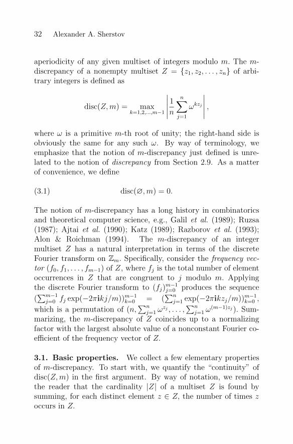
the m-discrepancy of a nonempty multiset Z = z1, z2, . . . , zn isdefined as
disc(Z,m) = maxk=1,2,...,m−1
∣∣∣∣∣ 1nn∑j=1
ωkzj
∣∣∣∣∣ ,where ω is a primitive m-th root of unity. This fundamentalquantity arises in combinatorics and theoretical computer science,e.g., Galil et al. (1989); Ruzsa (1987); Ajtai et al. (1990); Katz(1989); Razborov et al. (1993); Alon & Roichman (1994). Theidentity 1 + ω + ω2 + · · · + ωm−1 = 0 for any m-th root of unityω 6= 1 implies that the set Z = 0, 1, 2, . . . ,m − 1 achieves thesmallest possible m-discrepancy: disc(Z,m) = 0. Much sparsersets with small m-discrepancy can be shown to exist using theprobabilistic method (Fact 3.5 and Corollary 3.6). Specifically,one easily verifies for any constant ε > 0 the existence of a setZ ⊆ 0, 1, 2, . . . ,m − 1 with m-discrepancy at most ε and cardi-nality O(logm), an exponential improvement in sparsity comparedto the trivial set 0, 1, 2, . . . ,m− 1. We are aware of two efficientconstructions of sparse sets with small m-discrepancy, due to Aj-tai et al. (1990) and Katz (1989). The approach of Ajtai et al. iselementary except for an appeal to the prime number theorem,whereas Katz’s construction relies on deep results in number the-ory. Neither work appears to directly imply the kind of optimalde-randomization that we require, namely, an algorithm that runsin time polynomial in logm and produces a multiset of cardinalityO(logm) with m-discrepancy bounded away from 1. We obtainsuch an algorithm by adapting the approach of Ajtai et al. (1990).
The centerpiece of the construction of Ajtai et al. (1990) iswhat the authors call the iteration lemma, stated in this paper asTheorem 3.12. Its role is to reduce the construction of a sparse setwith small m-discrepancy to the construction of sparse sets withsmall p-discrepancy, for primes p m. Ajtai et al. (1990) provedtheir iteration lemma for m prime, but we show that their argu-ment readily generalizes to arbitrary moduli m. By applying theiteration lemma in a recursive manner, one reaches smaller andsmaller primes. Ajtai et al. (1990) continue this recursive processuntil they reach primes p so small that the trivial construction0, 1, 2, . . . , p − 1 can be considered sparse. We proceed differ-

The Hardest Halfspace 11
ently and terminate the recursion after just two stages, at whichpoint the input size is small enough for brute force search based onthe probabilistic method. The final set that we construct has sizelogarithmic in m and m-discrepancy a small constant, as opposedto the superlogarithmic size and o(1) discrepancy in the work ofAjtai et al. (1990).
We note that this modified approach additionally gives the firstexplicit circulant expander on n vertices of degree O(log n), whichis optimal and improves on the previous best degree bound of(log∗ n)O(log∗ n) · O(log n) due to Ajtai et al. (1990). Backgroundon circulant expanders, and the details of our expander construc-tion, can be found in Section 5.6.
Univariatization. We now describe the second major compo-nent of our proof. Consider a halfspace hn(x) = sgn(
∑zixi − θ)
in Boolean variables x1, x2, . . . , xn, where the coefficients can beassumed without loss of generality to be integers. Then the linearform
∑zixi − θ ranges in the discrete set ±1,±2, . . . ,±N, for
some integer N proportionate to the magnitude of the coefficients.As a result, one can approximate hn to any given error ε by approx-imating the sign function to ε on ±1,±2, . . . ,±N. This approachworks for both rational approximation and polynomial approxima-tion. We think of it as the black-box approach to the approximationof hn because it uses the linear form
∑zixi − θ rather than the
individual bits. There is no reason to expect that the black-boxconstruction is anywhere close to optimal. Indeed, there are half-spaces (Sherstov 2013a, Section 1.3) that can be approximated toarbitrarily small error by a rational function of degree 1 but requirea black-box approximant of degree Ω(n). Surprisingly, we are ableto construct a halfspace hn with exponentially large coefficientsfor which the black-box approximant is essentially optimal. As aresult, tight lower bounds for the rational and polynomial approxi-mation of hn follow immediately from the univariate lower boundsfor approximating the sign function on ±1,±2,±3, . . . ,±2Θ(n).The role of hn is to reduce the multivariate problem taken up inthis work to a well-understood univariate question, hence the termunivariatization.
The construction of hn involves several steps. First, we study
12 Alexander A. Sherstov
the probability distribution of the weighted sum z1X1 + z2X2 +· · · + znXn modulo m, where z1, z2, . . . , zn are given integers andthe bits X1, X2, . . . , Xn ∈ 0, 1 are chosen uniformly at random.We show that the distribution is exponentially close to uniformwhenever the multiset z1, z2, . . . , zn has m-discrepancy boundedaway from 1 (Lemma 4.3). For the next step, fix any multisetz1, z2, . . . , zn with small m-discrepancy and consider the linearmap L : 0, 1n → Zm given by L(x) =
∑zixi. At this point in
the proof, we know that for uniformly random X ∈ 0, 1n, theprobability distribution of L(X) is exponentially close to uniform.This implies that the characteristic functions of
L−1(0), L−1(1), . . . , L−1(m− 1)
have approximately the same Fourier spectrum up to degree cn, forsome constant c > 0. We substantially strengthen this conclusionby proving that there are probability distributions µ0, µ1, . . . , µm−1,supported on L−1(0), L−1(1), . . . , L−1(m − 1), respectively, suchthat the Fourier spectra of µ0, µ1, . . . , µm−1 are exactly the sameup to degree cn. Our proof relies on a general tool from Sherstov(2013b, Theorem 4.1), proved there using the Gershgorin circletheorem.
As our final step, we use µ0, µ1, . . . , µm−1 to construct a half-space in terms of z1, z2, . . . , zn whose approximation by rationalfunctions and polynomials gives corresponding approximants forthe sign function on the discrete set ±1,±2, . . . ,±m. More gen-erally, for any tuple z1, z2, . . . , zn, we define an associated half-space and prove a lower bound on m in terms of the discrepancyof the multiset z1, z2, . . . , zn. Combining this result with the ef-ficient construction of an integer set with small m-discrepancyfor m = 2Θ(n), we obtain an explicit halfspace hn : 0, 1n →−1,+1 whose approximation by polynomials and rational func-tions is equivalent to the univariate approximation of the sign func-tion on ±1,±2,±3, . . . ,±2Θ(n). Theorem 1.2 now follows by ap-pealing to known lower bounds for the polynomial and rationalapproximation of the sign function. To obtain the exponentialseparation of communication complexity with unbounded versusweakly unbounded error (Theorem 1.3), we use the pattern matrix
The Hardest Halfspace 13
method (Sherstov 2009b, 2011) to “lift” the lower bound of Theo-rem 1.2 to a discrepancy bound. Finally, our result on the thresholddegree of the intersection of two halfspaces (Theorem 1.6) worksby combining the rational approximation lower bound of Theo-rem 1.2 with a structural result from Sherstov (2013a) on the sign-representation of arbitrary functions of the form f ∧ f.
A key technical contribution of this paper is the identificationof m-discrepancy as a pseudorandom property that is weak enoughto admit efficient de-randomization and strong enough to allow theunivariatization of the corresponding halfspace. The previous, ex-istential result in Sherstov (2013b) used a completely different andmore complicated pseudorandom property based on affine shifts ofthe Fourier transform on 0, 1n, which we have not been able tode-randomize. Apart from the construction of a low-discrepancyset, our proof is simpler and more intuitive than the existentialproof in Sherstov (2013b).
1.5. Recent progress. Following up on our work, Hatami et al.(2020) recently obtained a sharper version of Theorem 1.3. Specif-ically, Hatami et al. (2020) constructed a communication problemFn : 0, 1n × 0, 1n → −1,+1 with sign-rank 3 and discrep-ancy exp(−Ω(n)). This gives a separation of O(1) versus Ω(n) forcommunication with unbounded versus weakly unbounded error,improving on our O(log n) versus Ω(n) separation. However, thework of Hatami et al. (2020) does not generalize to multipartycommunication and does not recover our approximation-theoreticresults for halfspaces. In particular, Theorem 1.2, Theorem 1.5,and Theorem 1.6 remain the strongest to date.
2. Preliminaries
We start with a review of the technical preliminaries. The purposeof this section is to make the paper as self-contained as possible,and comfortably readable by a broad audience. The expert readershould therefore skim this section for notation or skip it altogether.
2.1. Notation. There are two common arithmetic encodings forthe Boolean values: the traditional encoding false ↔ 0, true ↔ 1,
14 Alexander A. Sherstov
and the Fourier-motivated encoding false ↔ 1, true ↔ −1.Throughout this manuscript, we use the former encoding forthe domain of a Boolean function and the latter for the range.With this convention, Boolean functions are mappings 0, 1n →−1,+1 for some n. For Boolean functions f : 0, 1n → −1,+1and g : 0, 1m → −1,+1, we let f g denote the coordinatewisecomposition of f with g. Formally, f g : (0, 1m)n → −1,+1is given by
(2.1) (f g)(x1, x2, . . . , xn)
= f
(1− g(x1)
2,1− g(x2)
2, . . . ,
1− g(xn)
2
),
where the linear map on the right-hand side serves the purposeof switching between the distinct arithmetizations for the domainversus range. A partial function f on a set X is a function whosedomain of definition, denoted dom f, is a nonempty proper subsetof X. We generalize coordinatewise composition f g to partialBoolean functions f and g in the natural way. Specifically, f gis the Boolean function given by (2.1), with domain the set of allinputs (. . . , xi, . . . ) ∈ (dom g)n for which (. . . , (1− g(xi))/2, . . . ) ∈dom f.
We use the following two versions of the sign function:
sgnx =
−1 if x < 0,
0 if x = 0,
1 if x > 0,
sgnx =
−1 if x < 0,
1 if x > 0.
For a subset X ⊆ R, we let sgn |X denote the restriction of thesign function to X . A halfspace for us is any Boolean functionh : 0, 1n → −1,+1 given by
h(x) = sgn
(n∑i=1
wixi − θ
)
for some reals w1, w2, . . . , wn, θ. The majority function
The Hardest Halfspace 15
MAJn : 0, 1n → −1,+1 is the halfspace defined by
MAJn(x) = − sgn
(n∑i=1
xi −n
2− 1
4
)
=
−1 if x1 + x2 + · · ·+ xn > n/2,
1 otherwise.
Some authors define MAJn only for n odd, in which case thetiebreaker term 1/4 can be omitted.
The complement and the power set of a set S are denoted asusual by S and P(S), respectively. The symmetric difference ofsets S and T is S ⊕ T = (S ∩ T ) ∪ (S ∩ T ). Throughout thismanuscript, we use brace notation as in z1, z2, . . . , zn to specifymultisets rather than sets. The cardinality |Z| of a finite mul-tiset Z is defined as the total number of element occurrences inZ, with each element counted as many times as it occurs. Theequality and subset relations on multisets are defined analogously,with the number of element occurrences taken into account. Forexample, 1, 1, 2 = 1, 2, 1 but 1, 1, 2 6= 1, 2. Similarly,1, 2 ⊆ 1, 1, 2 but 1, 1, 2 * 1, 2.
The infinity norm of a function f : X → R is denoted ‖f‖∞ =supx∈X |f(x)|. For real-valued functions f and g and a nonemptyfinite subset X of their domain, we write
〈f, g〉X =1
|X |∑x∈X
f(x)g(x).
We will often use this notation with X a nonempty proper sub-set of the domain of f and g. We let ln x and log x stand for thenatural logarithm of x and the logarithm of x to base 2, respec-tively. The binary entropy function H : [0, 1] → [0, 1] is given byH(p) = −p log p − (1 − p) log(1 − p) and is strictly increasing on[0, 1/2]. The following bound is well known (Jukna 2001, p. 283):
k∑i=0
(n
i
)6 2H(k/n)n, k = 0, 1, 2, . . . ,
⌊n2
⌋.(2.2)
16 Alexander A. Sherstov
For a complex number x, we denote the real part, imaginary part,and complex conjugate of x as usual by Re(x), Im(x), and x, respec-tively. We typeset the imaginary unit i in boldface to distinguishit from the index variable i.
For an arbitrary integer a and a positive integer m, recall thata mod m denotes the unique element of 0, 1, 2, . . . ,m − 1 thatis congruent to a modulo m. For an integer m > 2, the symbolsZm and Z∗m refer to the ring of integers modulo m and the multi-plicative group of integers modulo m, respectively. For a multisetZ = z1, z2, . . . , zn of integers, we adopt the standard notation
−Z = −z1, . . . ,−zn,(2.3)
aZ = az1, . . . , azn,(2.4)
Z + b = z1 + b, . . . , zn + b,(2.5)
Z mod m = z1 mod m, . . . , zn mod m.(2.6)
Note that the multisets in (2.3)–(2.6) each have cardinality n, thesame as the original set Z. We often use these shorthands in com-bination, as in (aZ + b) mod m = (az1 + b) mod m, . . . , (azn +b) mod m.
For a logical condition C, we use the Iverson bracket
I[C] =
1 if C holds,
0 otherwise.
The following concentration inequality, due to Hoeffding (1963), iswell-known.
Fact 2.7 (Hoeffding’s Inequality). Let X1, X2, . . . , Xn be inde-pendent random variables with Xi ∈ [ai, bi]. Let
p =n∑i=1
EXi.
Then
P
[∣∣∣∣∣n∑i=1
Xi − p
∣∣∣∣∣ > δ
]6 2 exp
(− 2δ2∑n
i=1(bi − ai)2
).
In Fact 2.7 and throughout this paper, we typeset random variablesusing capital letters.
The Hardest Halfspace 17
2.2. Number-theoretic preliminaries. For positive integersa and b that are relatively prime, (a−1)b ∈ 1, 2, . . . , b− 1 denotesthe multiplicative inverse of a modulo b. The following fact is well-known and straightforward to verify; cf. Ajtai et al. (1990).
Fact 2.8. For any positive integers a and b that are relativelyprime,
(2.9)(a−1)bb
+(b−1)aa− 1
ab∈ Z.
Proof. We have a(a−1)b + b(b−1)a ≡ b(b−1)a ≡ 1 (mod a),and analogously a(a−1)b + b(b−1)a ≡ a(a−1)b ≡ 1 (mod b). Thus,a(a−1)b + b(b−1)a− 1 is divisible by both a and b. Since a and b arerelatively prime, we conclude that a(a−1)b + b(b−1)a− 1 is divisibleby ab, which is equivalent to (2.9).
Recall that the prime counting function π(x) for a real argumentx > 0 evaluates to the number of prime numbers less than or equalto x. In what follows, it will be clear from the context whether πrefers to 3.14159 . . . or the prime counting function. The asymp-totic growth of the latter is given by the prime number theorem,which states that π(n) ∼ n/ lnn. Many explicit bounds on π(n)are known, such as the following theorem of Rosser (1941).
Fact 2.10 (Rosser). For n > 55,
n
lnn+ 2< π(n) <
n
lnn− 4.
The number of distinct prime divisors of a natural number n isdenoted ν(n). We will need the following first-principles bound onν(n), which is asymptotically tight for infinitely many n.
Fact 2.11. The number of distinct prime divisors of n obeys
(2.12) (ν(n) + 1)! 6 n.
In particular,
(2.13) ν(n) 6 (1 + o(1))lnn
ln lnn.
18 Alexander A. Sherstov
Proof. An integer n > 1 has by definition ν(n) distinct primedivisors. Letting pk denote the k-th prime, we have
lnn > ln p1p2 . . . pν(n)
>ν(n)∑k=1
ln(k + 1)
>∫ ν(n)
1
lnx dx
= ν(n) ln ν(n)− ν(n) + 1,
where the second step uses the trivial estimate pk > k + 1. Thesecond step in this derivation settles (2.12), whereas the last stepsettles (2.13).
2.3. Matrix analysis. For an arbitrary set X such as X = Cor X = −1, 1, the symbol Xn×m denotes the family of n × mmatrices with entries in X. The symbols In and Jn,m stand forthe order-n identity matrix and the n ×m matrix of all ones, re-spectively. When the dimensions of the matrix are clear from thecontext, we omit the subscripts and write simply I or J. The short-hand diag(d1, d2, . . . , dn) refers to the diagonal matrix with entriesd1, d2, . . . , dn on the diagonal:
diag(d1, d2, . . . , dn) =
d1 0 · · · 00 d2 · · · 0...
.... . .
...0 0 · · · dn
.For a matrix M = [Mi,j], recall that its complex conjugate is givenby M = [Mi,j]. The transpose and conjugate transpose of Mare denoted MT and M∗ = MT , respectively. The conjugation,transpose, and conjugate transpose operations apply as a specialcase to vectors, which we view as matrices with a single column.We use the familiar matrix norms ‖M‖∞ = max |Mij| and ‖M‖1 =∑|Mij|. Again, these definitions carry over to vectors as a special
case. A matrix M ∈ Cn×n is called unitary if MM∗ = M∗M = I.

The Hardest Halfspace 19
A circulant matrix is any matrix C ∈ Cm×m of the form
C =
c0 c1 c2 · · · cm−2 cm−1
cm−1 c0 c1 · · · cm−3 cm−2
cm−2 cm−1 c0 · · · cm−4 cm−3...
......
. . ....
...c2 c3 c4 · · · c0 c1
c1 c2 c3 · · · cm−1 c0
(2.14)
for some c0, c1, . . . , cm−1 ∈ C. Thus, every row of C is obtainedby a circular shift of the previous row one entry to the right. Welet circ(c0, c1, . . . , cm−1) denote the right-hand side of (2.14). Inthis notation, circ(1, 0, . . . , 0) = I and circ(1, 1, . . . , 1) = J. Theeigenvalues and eigenvectors of a circulant matrix are well-knownand straightforward to determine. For the reader’s convenience, weinclude the short derivation below in Fact 2.15 and Corollary 2.17.
Fact 2.15. Let C = circ(c0, c1, . . . , cm−1) be a circulant matrix.Then for every m-th root of unity ω, the vector
(2.16)
1ωω2
...ωm−1
is an eigenvector of C with eigenvalue
∑m−1j=0 cjω
j.
Proof. Let v denote the vector in (2.16). Then for k =1, 2, 3, . . . ,m,
(Cv)k =m−1∑j=0
c(j−k+1) mod m ωj
=
(m−1∑j=0
c(j−k+1) mod m ωj−k+1
)vk
20 Alexander A. Sherstov
=
(m−1∑j=0
c(j−k+1) mod m ω(j−k+1) mod m
)vk
=
(m−1∑j=0
cjωj
)vk,
where the third step uses ωm = 1.
As a corollary to Fact 2.15, one recovers the full complement ofeigenvalues for any circulant matrix C and furthermore learns thatC is unitarily similar to a diagonal matrix. In the statement below,recall that a primitive m-th root of unity is any generator, such asexp(2πi/m), for the multiplicative group of the roots of xm − 1 ∈C[x]. We further remind the reader that 1+ω+ω2 +· · ·+ωm−1 = 0for any m-th root of unity ω 6= 1.
Corollary 2.17. Let C = circ(c0, c1, . . . , cm−1) be a circulantmatrix. Let ω be a primitive m-th root of unity. Then the matrix
W = [ωjk/√m]j,k=0,1,...,m−1
is unitary and satisfies
(2.18) W ∗CW
= diag
(m−1∑j=0
cj,m−1∑j=0
cjωj,m−1∑j=0
cjω2j, . . . ,
m−1∑j=0
cjω(m−1)j
).
In particular, the eigenvalues of C, counting multiplicities, are
m−1∑j=0
cjωkj, k = 0, 1, 2, . . . ,m− 1.
Proof. For k, k′ = 0, 1, . . . ,m− 1, we have
m−1∑j=0
ωjk√m· ω
jk′
√m
=1
m
m−1∑j=0
ωj(k−k′)
=
1 if k = k′,
0 otherwise,
The Hardest Halfspace 21
where the second step is valid because ω is primitive and in par-ticular ωk 6= ωk
′. We conclude that
(2.19) WW ∗ = W ∗W = I.
Fact 2.15 implies that
CW = W diag
(m−1∑j=0
cj,m−1∑j=0
cjωj,m−1∑j=0
cjω2j, . . . ,
m−1∑j=0
cjω(m−1)j
),
which in light of (2.19) is equivalent to (2.18).
2.4. Polynomial approximation. Recall that the total degreeof a multivariate real polynomial p : Rn → R, denoted deg p, is thelargest degree of any monomial of p. We use the terms “degree”and “total degree” interchangeably. Let f : X → R be a givenfunction with domain X ⊆ Rn. For any d > 0, define
E(f, d) = infp‖f − p‖∞,
where the infimum is over real polynomials p of degree at most d.In words, E(f, d) is the least error in a pointwise approximation off by a polynomial of degree no greater than d. The ε-approximatedegree of f is the minimum degree of a polynomial p that approx-imates f pointwise within ε:
‖f − p‖∞ 6 ε.
In this overview, we focus on the polynomial approximation of thesign function. We start with an elementary construction of anapproximant due to Buhrman et al. (2007a).
Fact 2.20 (Buhrman et al.). For any N > 1 and 0 < ε < 1, thesign function can be approximated on [−N,−1] ∪ [1, N ] pointwiseto within ε by a polynomial of degree
O
(N2 log
2
ε
).
22 Alexander A. Sherstov
The degree upper bound in Fact 2.20 is not tight. Indeed, aquadratically stronger bound of O(N log(2/ε)) follows in a straight-forward manner from Jackson’s theorem in approximation the-ory (Rivlin 1981, Theorem 1.4). Our applications do not benefitfrom this improvement, however, and we opt for the constructionof Buhrman et al. (2007a) because of its striking simplicity. Forthe reader’s convenience, we provide their short proof below.
Proof (adapted from Buhrman et al.). For a positive integer d,consider the degree-d univariate polynomial
Bd(t) =d∑
i=dd/2e
(d
i
)ti(1− t)d−i.
In words, Bd(t) is the probability of observing at least as manyheads as tails in a sequence of d independent coin flips, each comingup heads with probability t. By Hoeffding’s inequality (Fact 2.7)for sufficiently large d = O(N2 log(2/ε)), the polynomial Bd sends[0, 1
2− 1
2N]→ [0, ε
2] and similarly [1
2+ 1
2N, 1]→ [1− ε
2, 1]. As a result,
the shifted and scaled polynomial 2Bd
(1
2N· t+ 1
2
)−1 approximates
the sign function pointwise on [−N,−1] ∪ [1, N ] within ε.
On the lower bounds side, Paturi proved that low-degree polyno-mials cannot approximate the majority function well. He in factobtained analogous results for all symmetric functions, but thespecial case of majority will be sufficient for our purposes.
Theorem 2.21 (Paturi). For some constant c > 0 and all integersn > 1,
E(MAJn, cn) >1
3.
The constant 1/3 in Paturi’s theorem can be replaced by any otherin (0, 1). His result is of interest to us because along with Fact 2.20,it implies a lower bound for the approximation of the sign functionon the discrete set of points ±1,±2, . . . ,±N for any N.
Proposition 2.22. For all positive integers N and d,
E(sgn |±1,±2,...,±N, d) > 1−O(d
N
)1/2
.
The Hardest Halfspace 23
Proof. Abbreviate ε = E(sgn |±1,±2,...,±N, d) and fix a poly-nomial p of degree at most d that approximates the sign functionon ±1,±2, . . . ,±N within ε. Fact 2.20 gives a polynomial s ofdegree O(1/(1 − ε)2) that sends [−1 − ε,−1 + ε] → [−4/3,−2/3]and [1− ε, 1 + ε] → [2/3, 4/3]. Then the composition of these twoapproximants obeys
maxt=±1,±2,...,±N
| sgn(t)− s(p(t))| 6 1
3.
This in turn gives an approximant for the majority function onn = b(N − 1)/2c bits:
maxx∈0,1n
∣∣∣∣∣MAJn(x)− s
(p
(2
n∑j=1
(−1)xj + 1
))∣∣∣∣∣= max
x∈0,1n
∣∣∣∣∣sgn
(2
n∑j=1
(−1)xj + 1
)− s
(p
(2
n∑j=1
(−1)xj + 1
))∣∣∣∣∣6 max
t=±1,±2,...,±N| sgn(t)− s(p(t))|
61
3.
In view of Paturi’s lower bound for the majority function (Theo-rem 2.21), the approximant s(p(2
∑(−1)xj + 1)) must have de-
gree Ω(n) = Ω(N). But this composition is a polynomial inx ∈ 0, 1n of degree deg s · deg p = O(d/(1 − ε)2). We concludethat d/(1− ε)2 > Ω(N), whence ε > 1−O(d/N)1/2.
2.5. Rational approximation. Consider a rational functionr(x) = p(x)/q(x), where p and q are polynomials on Rn. We referto the degrees of p and q as the numerator degree and denominatordegree, respectively, of r. The degree of r is, then, the maximum ofthe numerator and denominator degrees. For a function f : X → Rwith domain X ⊆ Rn, we define
R(f, d0, d1) = infp,q
supx∈X
∣∣∣∣f(x)− p(x)
q(x)
∣∣∣∣ ,(2.23)
where the infimum is over multivariate polynomials p and q ofdegree at most d0 and d1, respectively, such that q does not vanish
24 Alexander A. Sherstov
on X. In words, R(f, d0, d1) is the least error in an approximationof f by a multivariate rational function with numerator degreeand denominator degree at most d0 and d1, respectively. We willbe mostly working with R(f, d0, d1) in the regimes d0 = d1 andd0 d1. In the former regime, we use the shorthand
R(f, d) = R(f, d, d).
As a limiting case of the latter regime, we have
E(f, d) = R(f, d, 0).
The study of the rational approximation of the sign functiondates back to the seminal work by Zolotarev (1877) in the 1870s.The problem was revisited almost a century later by Newman(1964), who proved the following result.
Fact 2.24 (Newman). For any N > 1 and any integer d > 1,
R(sgn |[−N,−1]∪[1,N ], d) 6 1− 1
N1/d.
For a recent exposition of Newman’s construction, we refer thereader to Sherstov (2013a, Theorem 2.4). As an important specialcase, Newman’s work gives upper bounds for the rational approxi-mation of the sign function on the discrete set ±1,±2, . . . ,±N.Newman’s upper bounds were sharpened and complemented withmatching lower bounds in Sherstov (2013a, Eq. (2.2) and Theo-rem 5.1), to the following effect.
Theorem 2.25 (Sherstov). For any positive integers N and d,
R(sgn |±1,±2,...,±N, d) =
1−N−Θ(1/d) if 1 6 d 6 logN,
2−Θ(d/ log(N/d)) if logN < d < N/2.
Among other things, Theorem 2.25 implies the following resulton the rational approximation of the majority function (Sherstov2013a, Eq. (2.2) and Theorems 5.1, 5.9).
The Hardest Halfspace 25
Theorem 2.26 (Sherstov). For any positive integers n and d,
R(MAJn, d) =
1− n−Θ(1/d) if 1 6 d 6 log n,
2−Θ(d/ log(n/d)) if log n 6 d < bn/4c.
2.6. Sign-representation. Let f : X → −1,+1 be a givenfunction, where X ⊂ Rn is finite. The threshold degree of f,denoted deg±(f), is the least degree of a polynomial p(x) suchthat f(x) ≡ sgn p(x). For functions f : X → −1,+1 andg : Y → −1,+1, we let the symbol f ∧ g stand for the func-tion X × Y → −1,+1 given by (f ∧ g)(x, y) = f(x) ∧ g(y).Note that in this notation, f and f ∧ f are completely differentfunctions, the former having domain X and the latter X ×X. Thefollowing ingenious observation, due to Beigel et al. (1995), relatesthe notions of sign-representation and rational approximation forconjunctions of Boolean functions.
Theorem 2.27 (Beigel et al.). Let f : X → −1,+1 andg : Y → −1,+1 be given functions, where X, Y ⊆ Rn. Let dbe any integer with
R(f, d) +R(g, d) < 1.
Then
deg±(f ∧ g) 6 4d.
Proof (adapted from Beigel et al.). Fix arbitrary rational func-tions p1(x)/q1(x) and p2(y)/q2(y) of degree at most d such that
supX
∣∣∣∣f(x)− p1(x)
q1(x)
∣∣∣∣+ supY
∣∣∣∣g(y)− p2(y)
q2(y)
∣∣∣∣ < 1.
Then
f(x) ∧ g(y) ≡ sgn(1 + f(x) + g(y))
≡ sgn
(1 +
p1(x)
q1(x)+p2(y)
q2(y)
).
Multiplying through by the positive quantity q1(x)2q2(y)2 givesthe desired sign-representing polynomial: f(x) ∧ g(y) ≡sgnq1(x)2q2(y)2 + p1(x)q1(x)q2(y)2 + p2(y)q2(y)q1(x)2.
26 Alexander A. Sherstov
The construction of Theorem 2.27 is somewhat ad hoc, and thereis no particular reason to believe that it gives a sign-representingpolynomial of asymptotically optimal degree. Remarkably, it does.The following converse to the theorem of Beigel et al. was estab-lished by Sherstov (2013a, Theorem 3.16).
Theorem 2.28 (Sherstov). Let f : X → −1,+1 and g : Y →−1,+1 be given functions, where X, Y ⊂ Rn are arbitrary finitesets. Assume that f and g are not identically false. Let d =deg±(f ∧ g). Then
R(f, 4d) +R(g, 2d) < 1.
2.7. Symmetrization. Let Sn denote the symmetric group onn elements. For σ ∈ Sn and x ∈ 0, 1n, we denote σx =(xσ(1), . . . , xσ(n)) ∈ 0, 1n. For x ∈ 0, 1n, we define |x| =x1 +x2 + · · ·+xn. A function φ : 0, 1n → R is called symmetric ifφ(x) = φ(σx) for every x ∈ 0, 1n and every σ ∈ Sn. Equivalently,φ is symmetric if φ(x) is uniquely determined by |x|. Symmetricfunctions on 0, 1n are intimately related to univariate polyno-mials, as borne out by the symmetrization argument (Minsky &Papert 1969).
Proposition 2.29 (Minsky and Papert). Let p : 0, 1n → R bea polynomial of degree d. Then there is a univariate polynomial p∗
of degree at most d such that for all x ∈ 0, 1n,
Eσ∈Sn
p(σx) = p∗(|x|).
Minsky and Papert’s result generalizes to block-symmetric func-tions, as pointed out by Razborov & Sherstov (2010, Proposi-tion 2.3):
Proposition 2.30 (Razborov and Sherstov). Let n1, . . . , nkbe positive integers. Let p : 0, 1n1 × · · · × 0, 1nk → R be apolynomial of degree d. Then there is a polynomial p∗ : Rk → R ofdegree at most d such that for all x1 ∈ 0, 1n1 , . . . , xk ∈ 0, 1nk ,
Eσ1∈Sn1 ,...,σk∈Snk
p(σ1x1, . . . , σkxk) = p∗(|x1|, . . . , |xk|).
The Hardest Halfspace 27
Proposition 2.30 follows in a straightforward manner from Min-sky and Papert’s Proposition 2.29 by induction on the number ofblocks k.
2.8. Communication complexity. An excellent reference oncommunication complexity is the monograph by Kushilevitz &Nisan (1997). In this overview, we will limit ourselves to key def-initions and notation. We adopt the randomized number-on-the-forehead model, due to Chandra et al. (1983). The model features kcommunicating players, tasked with computing a (possibly partial)Boolean function F on the Cartesian product X1 ×X2 × · · · ×Xk
of some finite sets X1, X2, . . . , Xk. A given input (x1, x2, . . . , xk) ∈X1 × X2 × · · · × Xk is distributed among the players by placingxi, figuratively speaking, on the forehead of the i-th player (fori = 1, 2, . . . , k). In other words, the i-th player knows the argu-ments x1, . . . , xi−1, xi+1, . . . , xk but not xi. The players communi-cate by sending broadcast messages, taking turns according to aprotocol agreed upon in advance. Each of them privately holdsan unlimited supply of uniformly random bits, which he can usealong with his available arguments when deciding what messageto send at any given point in the protocol. The protocol’s pur-pose is to allow accurate computation of F everywhere on thedomain of F . An ε-error protocol for F is one which, on ev-ery input (x1, x2, . . . , xk) ∈ domF, produces the correct answerF (x1, x2, . . . , xk) with probability at least 1− ε. The cost of a pro-tocol is the total bit length of the messages broadcast by all theplayers in the worst case; here the contribution of a b-bit broadcastto the protocol cost is b rather than k · b. The ε-error randomizedcommunication complexity of F, denoted Rε(F ), is the least costof an ε-error randomized protocol for F . As a special case of thismodel for k = 2, one recovers the original two-party model of Yao(1979) reviewed in the introduction.
We focus on randomized protocols with probability of errorclose to that of random guessing, 1/2. There are two natural waysto define the communication complexity of a multiparty problemF in this setting. The communication complexity of F with un-bounded error, introduced by Paturi & Simon (1986), is the quan-
28 Alexander A. Sherstov
tityUPP(F ) = inf
06ε<1/2Rε(F ).
The error probability in this formalism is “unbounded” in the sensethat it can be arbitrarily close to 1/2. Babai et al. (1986) proposedan alternate quantity, which includes an additive penalty term thatdepends on the error probability:
PP(F ) = inf06ε<1/2
Rε(F ) + log
112− ε
.
We refer to PP(F ) as the communication complexity of F withweakly unbounded error. These two complexity measures naturallygive rise to corresponding complexity classes UPPk and PPk inmultiparty communication complexity (Babai et al. 1986), bothinspired by Gill’s probabilistic polynomial time for Turing ma-chines (Gill 1977). Formally, let Fn,k∞n=1 be a family of k-partycommunication problems Fn,k : (0, 1n)k → −1,+1, where k =k(n) is either a constant or a function. Then Fn,k∞n=1 ∈ UPPk ifand only if UPP(Fn,k) 6 logc n for some constant c and all n > c.Analogously, Fn,k∞n=1 ∈ PPk if and only if PP(Fn,k) 6 logc n forsome constant c and all n > c. By definition,
PPk ⊆ UPPk.
It is standard practice to abbreviate PP = PP2 and UPP = UPP2.The following well-known fact, whose proof in the stated gener-ality is available in Sherstov (2018, Fact 2.4), gives a large classof communication problems that are efficiently computable withunbounded error.
Fact 2.31. Let F : (0, 1n)k → −1,+1 be a k-party commu-nication problem such that F (x) = sgn p(x) for some polynomialp with ` monomials. Then
UPP(F ) 6 dlog `e+ 2.
In the setting of k = 2 parties, Paturi & Simon (1986) showedthat unbounded-error communication complexity has a natural
The Hardest Halfspace 29
matrix-analytic characterization. For a matrix M without zeroentries, the sign-rank of M is denoted rk±(M) and defined as theminimum rank of a real matrix R such that sgnRi,j = sgnMi,j forall i, j. In words, the sign-rank of M is the minimum rank of a realmatrix that has the same sign pattern as M. We extend the notionof sign-rank to communication problems F : X × Y → −1,+1by defining rk±(F ) = rk±(MF ), where MF = [F (x, y)]x∈X,y∈Y isthe characteristic matrix of F. The following classic result due toPaturi & Simon (1986, Theorem 3) relates two-party unbounded-error communication complexity to sign-rank.
Theorem 2.32 (Paturi and Simon). Let F : X×Y → −1,+1be a two-party communication problem. Then
log rk±(F ) 6 UPP(F ) 6 log rk±(F ) + 2.
2.9. Discrepancy. A k-dimensional cylinder intersection is afunction χ : X1 ×X2 × · · · ×Xk → 0, 1 of the form
χ(x1, x2, . . . , xk) =k∏i=1
χi(x1, . . . , xi−1, xi+1, . . . , xk),
where χi : X1×· · ·×Xi−1×Xi+1×· · ·×Xk → 0, 1. In other words,a k-dimensional cylinder intersection is the product of k functionswith range 0, 1, where the i-th function does not depend on thei-th coordinate but may depend arbitrarily on the other k−1 coor-dinates. Introduced by Babai et al. (1992), cylinder intersectionsare the fundamental building blocks of communication protocolsand for that reason play a central role in the theory. For a (pos-sibly partial) Boolean function F on X1 × X2 × · · · × Xk and aprobability distribution P on X1 ×X2 × · · · ×Xk, the discrepancyof F with respect to P is given by
discP (F ) =∑
x/∈domF
P (x) + maxχ
∣∣∣∣∣ ∑x∈domF
F (x)P (x)χ(x)
∣∣∣∣∣ ,where the maximum is over cylinder intersections χ. The minimumdiscrepancy over all distributions is denoted
disc(F ) = minP
discP (F ).
30 Alexander A. Sherstov
Upper bounds on a function’s discrepancy give lower bounds on itsrandomized communication complexity, a classic technique knownas the discrepancy method (Chor & Goldreich 1988; Babai et al.1992; Kushilevitz & Nisan 1997).
Theorem 2.33. Let F be a (possibly partial) Boolean functionon X1 ×X2 × · · · ×Xk. Then for 0 6 ε 6 1/2,
2Rε(F ) >1− 2ε
disc(F ).
A proof of Theorem 2.33 in the stated generality is availablein Sherstov (2016, Theorem 2.9). Combining this theorem withthe definition of PP(F ) gives the following corollary.
Corollary 2.34. Let F be a (possibly partial) Boolean functionon X1 ×X2 × · · · ×Xk. Then
PP(F ) > log2
disc(F ).
2.10. Pattern matrix method. Theorem 2.33 and Corol-lary 2.34 highlight the role of discrepancy in proving lower boundson randomized communication complexity. Apart from a fewcanonical examples (Kushilevitz & Nisan 1997), discrepancy is achallenging quantity to analyze. The pattern matrix method is atechnique that gives tight bounds on the discrepancy and commu-nication complexity for a large class of communication problems.The technique was developed by Sherstov (2009b, 2011) for two-party communication complexity and has since been generalizedby several authors to the multiparty setting. We now review thestrongest form (Sherstov 2016, 2014) of the pattern matrix method,focusing our discussion on discrepancy bounds.
Set disjointness is the k-party communication problem of deter-mining whether k given subsets of the universe 1, 2, . . . , n haveempty intersection, where, as usual, the i-th party knows all thesets except for the i-th. Identifying the sets with their character-istic vectors, set disjointness corresponds to the Boolean function
The Hardest Halfspace 31
DISJn,k : (0, 1n)k → −1,+1 given by
DISJn,k(x1, x2, . . . , xk) = ¬n∨i=1
x1,i ∧ x2,i ∧ · · · ∧ xk,i .(2.35)
The partial function UDISJn,k on (0, 1n)k, called unique set dis-jointness, is defined as DISJn,k with domain restricted to inputsx ∈ (0, 1n)k such that x1,i ∧ x2,i ∧ · · · ∧ xk,i = 1 for at most onecoordinate i. In set-theoretic terms, this restriction corresponds torequiring that the k sets either have empty intersection or intersectin a unique element.
The pattern matrix method pertains to the communicationcomplexity of composed communication problems. Specifically,let G be a (possibly partial) Boolean function on X1 × X2 ×· · · × Xk, representing a k-party communication problem, andlet f : 0, 1n → −1,+1 be given. The coordinatewise com-position f G is then a k-party communication problem onXn
1 × Xn2 × · · · × Xn
k . We are now in a position to state the pat-tern matrix method for discrepancy bounds (Sherstov 2016, The-orem 5.7).
Theorem 2.36 (Sherstov). For every Boolean functionf : 0, 1n → −1,+1, all positive integers m and k, and all reals0 < γ < 1,
disc(f UDISJm,k) 6
(e · 2kn
deg1−γ(f)√m
)deg1−γ(f)
+ γ .
This theorem makes it possible to prove communication lowerbounds by leveraging the existing literature on polynomial approx-imation. In follow-up work, the author improved Theorem 2.36 toan essentially tight upper bound (Sherstov 2014, Theorem 5.7).However, we will not need this sharper version.
3. Discrepancy of integer sets
Let m > 2 be an integer modulus. Key to our work is the no-tion of m-discrepancy, which quantifies the pseudorandomness or
32 Alexander A. Sherstov
aperiodicity of any given multiset of integers modulo m. The m-discrepancy of a nonempty multiset Z = z1, z2, . . . , zn of arbi-trary integers is defined as
disc(Z,m) = maxk=1,2,...,m−1
∣∣∣∣∣ 1nn∑j=1
ωkzj
∣∣∣∣∣ ,where ω is a primitive m-th root of unity; the right-hand side isobviously the same for any such ω. By way of terminology, weemphasize that the notion of m-discrepancy just defined is unre-lated to the notion of discrepancy from Section 2.9. As a matterof convenience, we define
(3.1) disc(∅,m) = 0.
The notion of m-discrepancy has a long history in combinatoricsand theoretical computer science, e.g., Galil et al. (1989); Ruzsa(1987); Ajtai et al. (1990); Katz (1989); Razborov et al. (1993);Alon & Roichman (1994). The m-discrepancy of an integermultiset Z has a natural interpretation in terms of the discreteFourier transform on Zm. Specifically, consider the frequency vec-tor (f0, f1, . . . , fm−1) of Z, where fj is the total number of elementoccurrences in Z that are congruent to j modulo m. Applyingthe discrete Fourier transform to (fj)
m−1j=0 produces the sequence
(∑m−1
j=0 fj exp(−2πikj/m))m−1k=0 = (
∑nj=1 exp(−2πikzj/m))m−1
k=0 ,
which is a permutation of (n,∑n
j=1 ωzj , . . . ,
∑nj=1 ω
(m−1)zj). Sum-marizing, the m-discrepancy of Z coincides up to a normalizingfactor with the largest absolute value of a nonconstant Fourier co-efficient of the frequency vector of Z.
3.1. Basic properties. We collect a few elementary propertiesof m-discrepancy. To start with, we quantify the “continuity” ofdisc(Z,m) in the first argument. By way of notation, we remindthe reader that the cardinality |Z| of a multiset Z is found bysumming, for each distinct element z ∈ Z, the number of times zoccurs in Z.
The Hardest Halfspace 33
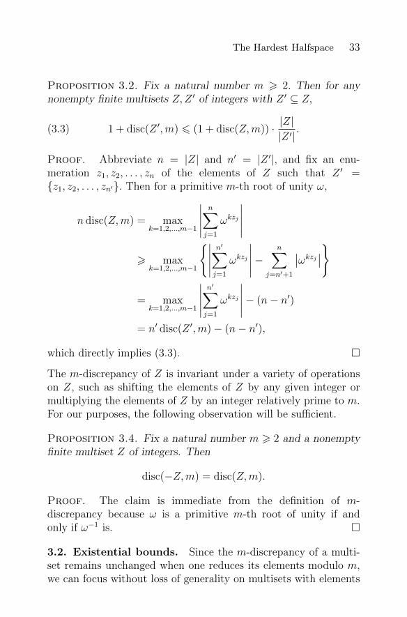
Proposition 3.2. Fix a natural number m > 2. Then for anynonempty finite multisets Z,Z ′ of integers with Z ′ ⊆ Z,
(3.3) 1 + disc(Z ′,m) 6 (1 + disc(Z,m)) · |Z||Z ′|
.
Proof. Abbreviate n = |Z| and n′ = |Z ′|, and fix an enu-meration z1, z2, . . . , zn of the elements of Z such that Z ′ =z1, z2, . . . , zn′. Then for a primitive m-th root of unity ω,
n disc(Z,m) = maxk=1,2,...,m−1
∣∣∣∣∣n∑j=1
ωkzj
∣∣∣∣∣> max
k=1,2,...,m−1
∣∣∣∣∣n′∑j=1
ωkzj
∣∣∣∣∣−n∑
j=n′+1
∣∣ωkzj ∣∣
= maxk=1,2,...,m−1
∣∣∣∣∣n′∑j=1
ωkzj
∣∣∣∣∣− (n− n′)
= n′ disc(Z ′,m)− (n− n′),
which directly implies (3.3).
The m-discrepancy of Z is invariant under a variety of operationson Z, such as shifting the elements of Z by any given integer ormultiplying the elements of Z by an integer relatively prime to m.For our purposes, the following observation will be sufficient.
Proposition 3.4. Fix a natural number m > 2 and a nonemptyfinite multiset Z of integers. Then
disc(−Z,m) = disc(Z,m).
Proof. The claim is immediate from the definition of m-discrepancy because ω is a primitive m-th root of unity if andonly if ω−1 is.
3.2. Existential bounds. Since the m-discrepancy of a multi-set remains unchanged when one reduces its elements modulo m,we can focus without loss of generality on multisets with elements
34 Alexander A. Sherstov
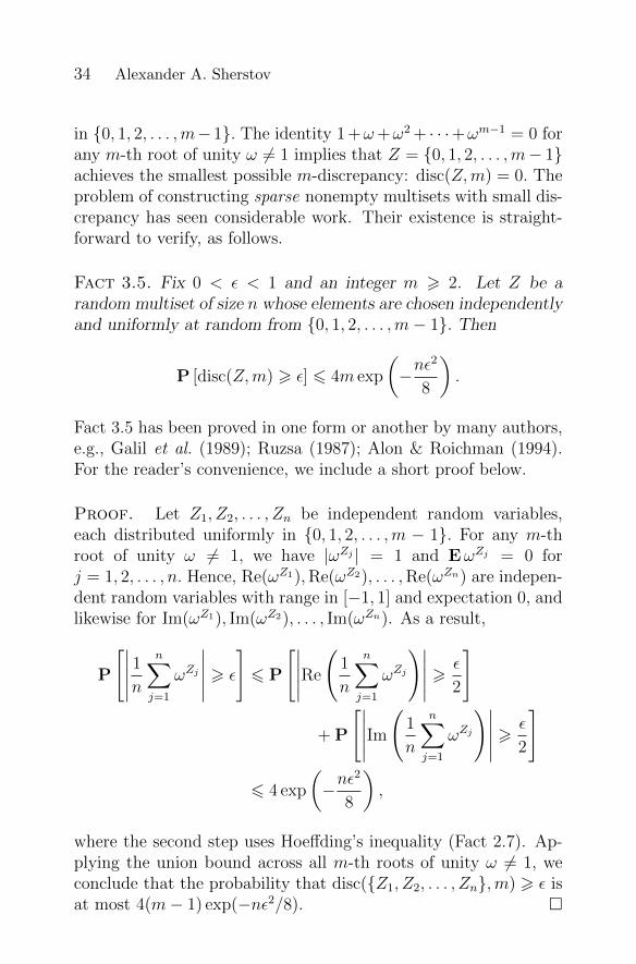
in 0, 1, 2, . . . ,m−1. The identity 1 +ω+ω2 + · · ·+ωm−1 = 0 forany m-th root of unity ω 6= 1 implies that Z = 0, 1, 2, . . . ,m− 1achieves the smallest possible m-discrepancy: disc(Z,m) = 0. Theproblem of constructing sparse nonempty multisets with small dis-crepancy has seen considerable work. Their existence is straight-forward to verify, as follows.
Fact 3.5. Fix 0 < ε < 1 and an integer m > 2. Let Z be arandom multiset of size n whose elements are chosen independentlyand uniformly at random from 0, 1, 2, . . . ,m− 1. Then
P [disc(Z,m) > ε] 6 4m exp
(−nε
2
8
).
Fact 3.5 has been proved in one form or another by many authors,e.g., Galil et al. (1989); Ruzsa (1987); Alon & Roichman (1994).For the reader’s convenience, we include a short proof below.
Proof. Let Z1, Z2, . . . , Zn be independent random variables,each distributed uniformly in 0, 1, 2, . . . ,m − 1. For any m-throot of unity ω 6= 1, we have |ωZj | = 1 and EωZj = 0 forj = 1, 2, . . . , n. Hence, Re(ωZ1),Re(ωZ2), . . . ,Re(ωZn) are indepen-dent random variables with range in [−1, 1] and expectation 0, andlikewise for Im(ωZ1), Im(ωZ2), . . . , Im(ωZn). As a result,
P
[∣∣∣∣∣ 1nn∑j=1
ωZj
∣∣∣∣∣ > ε
]6 P
[∣∣∣∣∣Re
(1
n
n∑j=1
ωZj
)∣∣∣∣∣ > ε
2
]
+ P
[∣∣∣∣∣Im(
1
n
n∑j=1
ωZj
)∣∣∣∣∣ > ε
2
]
6 4 exp
(−nε
2
8
),
where the second step uses Hoeffding’s inequality (Fact 2.7). Ap-plying the union bound across all m-th roots of unity ω 6= 1, weconclude that the probability that disc(Z1, Z2, . . . , Zn,m) > ε isat most 4(m− 1) exp(−nε2/8).
The Hardest Halfspace 35
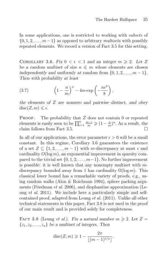
In some applications, one is restricted to working with subsets of0, 1, 2, . . . ,m−1 as opposed to arbitrary multisets with possiblyrepeated elements. We record a version of Fact 3.5 for this setting.
Corollary 3.6. Fix 0 < ε < 1 and an integer m > 2. Let Zbe a random multiset of size n 6 m whose elements are chosenindependently and uniformly at random from 0, 1, 2, . . . ,m− 1.Then with probability at least
(3.7)(
1− n
m
)n− 4m exp
(−nε
2
8
),
the elements of Z are nonzero and pairwise distinct, and obeydisc(Z,m) 6 ε.
Proof. The probability that Z does not contain 0 or repeatedelements is easily seen to be
∏ni=1
m−im> (1− n
m)n. As a result, the
claim follows from Fact 3.5.
In all of our applications, the error parameter ε > 0 will be a smallconstant. In this regime, Corollary 3.6 guarantees the existenceof a set Z ⊆ 1, 2, . . . ,m − 1 with m-discrepancy at most ε andcardinality O(logm), an exponential improvement in sparsity com-pared to the trivial set 0, 1, 2, . . . ,m−1. No further improvementis possible: it is well known that any nonempty multiset with m-discrepancy bounded away from 1 has cardinality Ω(logm). Thisclassical lower bound has a remarkable variety of proofs, e.g., us-ing random walks (Alon & Roichman 1994), sphere packing argu-ments (Friedman et al. 2006), and diophantine approximation (Le-ung et al. 2011). We include here a particularly simple and self-contained proof, adapted from Leung et al. (2011). Unlike all othertechnical statements in this paper, Fact 3.8 is not used in the proofof our main result and is provided solely for completeness.
Fact 3.8 (Leung et al.). Fix a natural number m > 2. Let Z =z1, z2, . . . , zn be a multiset of integers. Then
disc(Z,m) > 1− 2π
b(m− 1)1/nc.
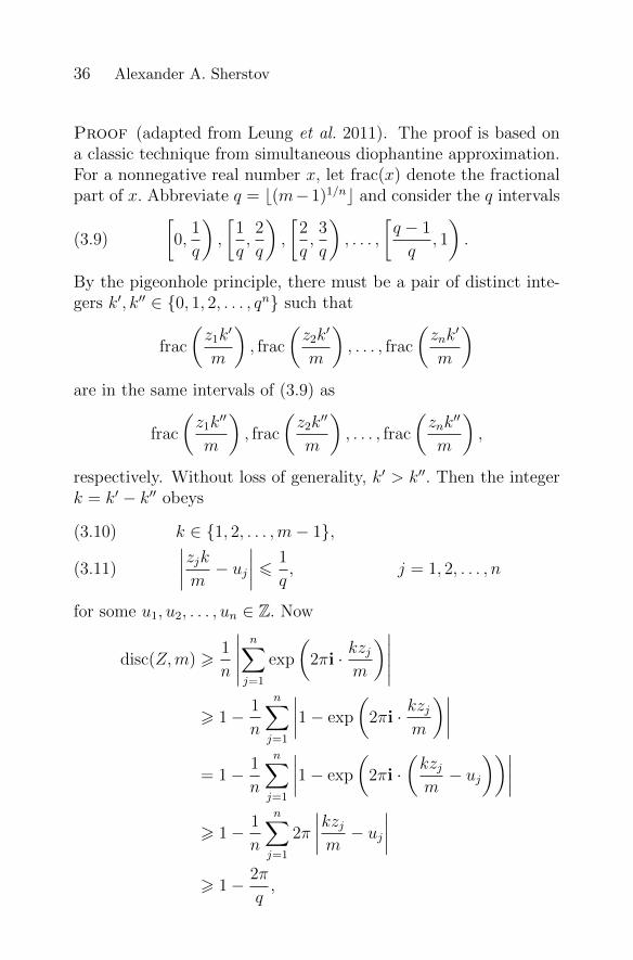
36 Alexander A. Sherstov
Proof (adapted from Leung et al. 2011). The proof is based ona classic technique from simultaneous diophantine approximation.For a nonnegative real number x, let frac(x) denote the fractionalpart of x. Abbreviate q = b(m−1)1/nc and consider the q intervals
(3.9)
[0,
1
q
),
[1
q,2
q
),
[2
q,3
q
), . . . ,
[q − 1
q, 1
).
By the pigeonhole principle, there must be a pair of distinct inte-gers k′, k′′ ∈ 0, 1, 2, . . . , qn such that
frac
(z1k′
m
), frac
(z2k′
m
), . . . , frac
(znk
′
m
)are in the same intervals of (3.9) as
frac
(z1k′′
m
), frac
(z2k′′
m
), . . . , frac
(znk
′′
m
),
respectively. Without loss of generality, k′ > k′′. Then the integerk = k′ − k′′ obeys
k ∈ 1, 2, . . . ,m− 1,(3.10) ∣∣∣∣zjkm − uj∣∣∣∣ 6 1
q, j = 1, 2, . . . , n(3.11)
for some u1, u2, . . . , un ∈ Z. Now
disc(Z,m) >1
n
∣∣∣∣∣n∑j=1
exp
(2πi · kzj
m
)∣∣∣∣∣> 1− 1
n
n∑j=1
∣∣∣∣1− exp
(2πi · kzj
m
)∣∣∣∣= 1− 1
n
n∑j=1
∣∣∣∣1− exp
(2πi ·
(kzjm− uj
))∣∣∣∣> 1− 1
n
n∑j=1
2π
∣∣∣∣kzjm − uj∣∣∣∣
> 1− 2π
q,
The Hardest Halfspace 37
where the first step uses the definition of m-discrepancy; the sec-ond step applies the triangle inequality; the third step is validby periodicity; the fourth step uses the bound |1 − exp(2πxi)| =√
2− 2 cos(2πx) 6 2π|x| for all real x; and the final step is imme-diate from (3.11).
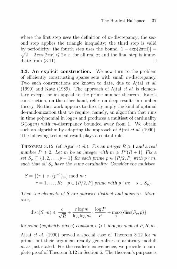
3.3. An explicit construction. We now turn to the problemof efficiently constructing sparse sets with small m-discrepancy.Two such constructions are known to date, due to Ajtai et al.(1990) and Katz (1989). The approach of Ajtai et al. is elemen-tary except for an appeal to the prime number theorem. Katz’sconstruction, on the other hand, relies on deep results in numbertheory. Neither work appears to directly imply the kind of optimalde-randomization that we require, namely, an algorithm that runsin time polynomial in logm and produces a multiset of cardinalityO(logm) with m-discrepancy bounded away from 1. We obtainsuch an algorithm by adapting the approach of Ajtai et al. (1990).The following technical result plays a central role.
Theorem 3.12 (cf. Ajtai et al.). Fix an integer R > 1 and a realnumber P > 2. Let m be an integer with m > P 2(R + 1). Fix aset Sp ⊆ 1, 2, . . . , p − 1 for each prime p ∈ (P/2, P ] with p - m,such that all Sp have the same cardinality. Consider the multiset
S = (r + s · (p−1)m) mod m :
r = 1, . . . , R; p ∈ (P/2, P ] prime with p - m; s ∈ Sp.
Then the elements of S are pairwise distinct and nonzero. More-over,
disc(S,m) 6c√R
+c logm
log logm· logP
P+ max
pdisc(Sp, p)
for some (explicitly given) constant c > 1 independent of P,R,m.
Ajtai et al. (1990) proved a special case of Theorem 3.12 for mprime, but their argument readily generalizes to arbitrary modulim as just stated. For the reader’s convenience, we provide a com-plete proof of Theorem 3.12 in Section 6. The theorem’s purpose is
38 Alexander A. Sherstov
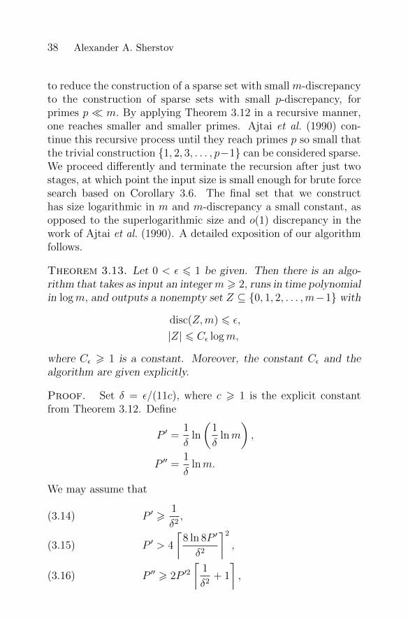
to reduce the construction of a sparse set with small m-discrepancyto the construction of sparse sets with small p-discrepancy, forprimes p m. By applying Theorem 3.12 in a recursive manner,one reaches smaller and smaller primes. Ajtai et al. (1990) con-tinue this recursive process until they reach primes p so small thatthe trivial construction 1, 2, 3, . . . , p−1 can be considered sparse.We proceed differently and terminate the recursion after just twostages, at which point the input size is small enough for brute forcesearch based on Corollary 3.6. The final set that we constructhas size logarithmic in m and m-discrepancy a small constant, asopposed to the superlogarithmic size and o(1) discrepancy in thework of Ajtai et al. (1990). A detailed exposition of our algorithmfollows.
Theorem 3.13. Let 0 < ε 6 1 be given. Then there is an algo-rithm that takes as input an integerm > 2, runs in time polynomialin logm, and outputs a nonempty set Z ⊆ 0, 1, 2, . . . ,m−1 with
disc(Z,m) 6 ε,
|Z| 6 Cε logm,
where Cε > 1 is a constant. Moreover, the constant Cε and thealgorithm are given explicitly.
Proof. Set δ = ε/(11c), where c > 1 is the explicit constantfrom Theorem 3.12. Define
P ′ =1
δln
(1
δlnm
),
P ′′ =1
δlnm.
We may assume that
P ′ >1
δ2,(3.14)
P ′ > 4
⌈8 ln 8P ′
δ2
⌉2
,(3.15)
P ′′ > 2P ′2⌈
1
δ2+ 1
⌉,(3.16)
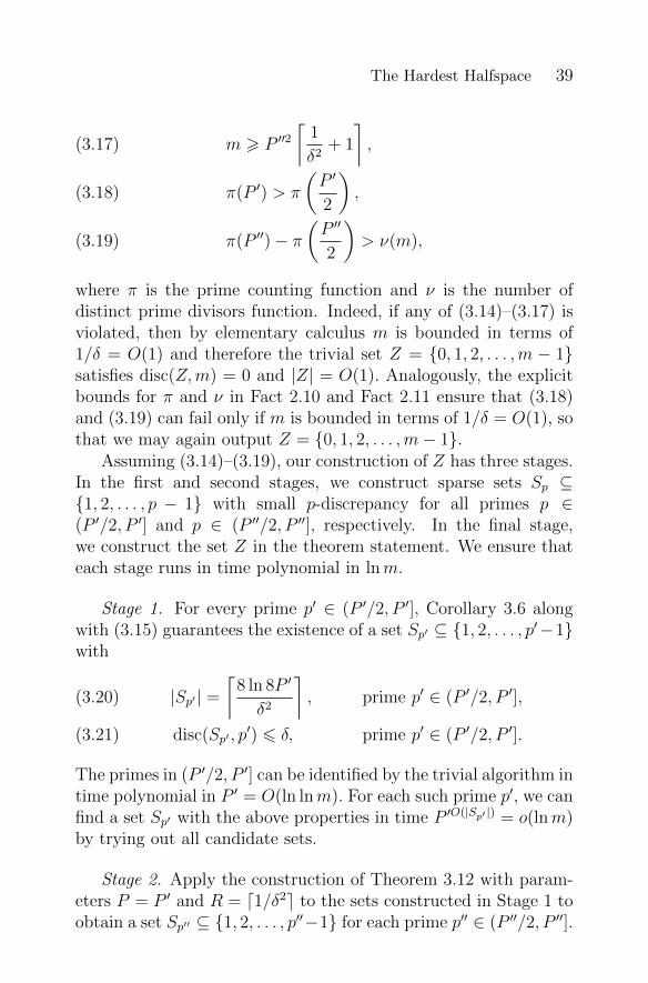
The Hardest Halfspace 39
m > P ′′2⌈
1
δ2+ 1
⌉,(3.17)
π(P ′) > π
(P ′
2
),(3.18)
π(P ′′)− π(P ′′
2
)> ν(m),(3.19)
where π is the prime counting function and ν is the number ofdistinct prime divisors function. Indeed, if any of (3.14)–(3.17) isviolated, then by elementary calculus m is bounded in terms of1/δ = O(1) and therefore the trivial set Z = 0, 1, 2, . . . ,m − 1satisfies disc(Z,m) = 0 and |Z| = O(1). Analogously, the explicitbounds for π and ν in Fact 2.10 and Fact 2.11 ensure that (3.18)and (3.19) can fail only if m is bounded in terms of 1/δ = O(1), sothat we may again output Z = 0, 1, 2, . . . ,m− 1.
Assuming (3.14)–(3.19), our construction of Z has three stages.In the first and second stages, we construct sparse sets Sp ⊆1, 2, . . . , p − 1 with small p-discrepancy for all primes p ∈(P ′/2, P ′] and p ∈ (P ′′/2, P ′′], respectively. In the final stage,we construct the set Z in the theorem statement. We ensure thateach stage runs in time polynomial in lnm.
Stage 1. For every prime p′ ∈ (P ′/2, P ′], Corollary 3.6 alongwith (3.15) guarantees the existence of a set Sp′ ⊆ 1, 2, . . . , p′−1with
|Sp′ | =⌈
8 ln 8P ′
δ2
⌉, prime p′ ∈ (P ′/2, P ′],(3.20)
disc(Sp′ , p′) 6 δ, prime p′ ∈ (P ′/2, P ′].(3.21)
The primes in (P ′/2, P ′] can be identified by the trivial algorithm intime polynomial in P ′ = O(ln lnm). For each such prime p′, we canfind a set Sp′ with the above properties in time P ′O(|Sp′ |) = o(lnm)by trying out all candidate sets.
Stage 2. Apply the construction of Theorem 3.12 with param-eters P = P ′ and R = d1/δ2e to the sets constructed in Stage 1 toobtain a set Sp′′ ⊆ 1, 2, . . . , p′′−1 for each prime p′′ ∈ (P ′′/2, P ′′].
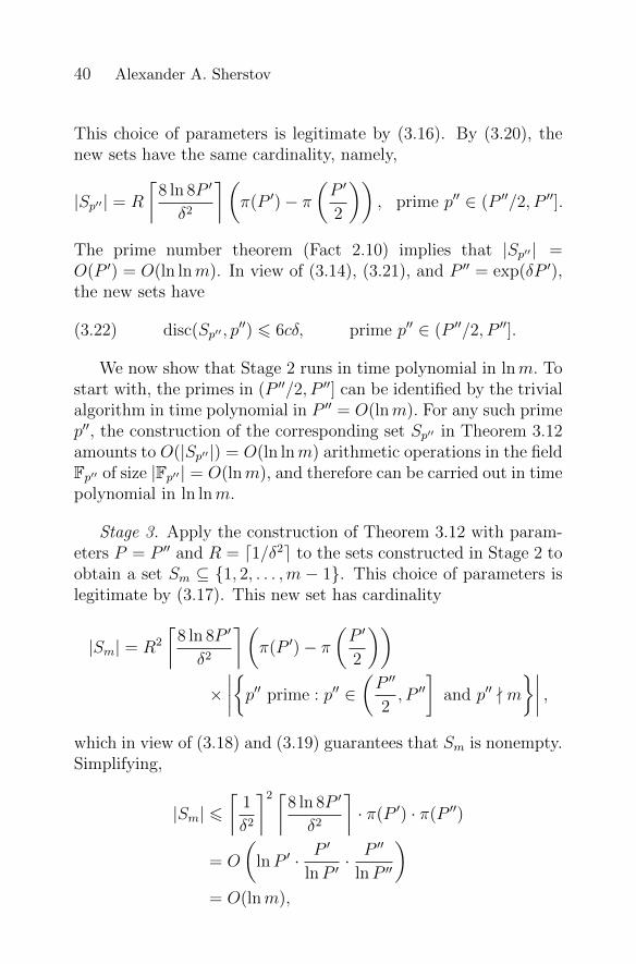
40 Alexander A. Sherstov
This choice of parameters is legitimate by (3.16). By (3.20), thenew sets have the same cardinality, namely,
|Sp′′| = R
⌈8 ln 8P ′
δ2
⌉(π(P ′)− π
(P ′
2
)), prime p′′ ∈ (P ′′/2, P ′′].
The prime number theorem (Fact 2.10) implies that |Sp′′ | =O(P ′) = O(ln lnm). In view of (3.14), (3.21), and P ′′ = exp(δP ′),the new sets have
disc(Sp′′ , p′′) 6 6cδ, prime p′′ ∈ (P ′′/2, P ′′].(3.22)
We now show that Stage 2 runs in time polynomial in lnm. Tostart with, the primes in (P ′′/2, P ′′] can be identified by the trivialalgorithm in time polynomial in P ′′ = O(lnm). For any such primep′′, the construction of the corresponding set Sp′′ in Theorem 3.12amounts to O(|Sp′′ |) = O(ln lnm) arithmetic operations in the fieldFp′′ of size |Fp′′| = O(lnm), and therefore can be carried out in timepolynomial in ln lnm.
Stage 3. Apply the construction of Theorem 3.12 with param-eters P = P ′′ and R = d1/δ2e to the sets constructed in Stage 2 toobtain a set Sm ⊆ 1, 2, . . . ,m − 1. This choice of parameters islegitimate by (3.17). This new set has cardinality
|Sm| = R2
⌈8 ln 8P ′
δ2
⌉(π(P ′)− π
(P ′
2
))×∣∣∣∣p′′ prime : p′′ ∈
(P ′′
2, P ′′
]and p′′ - m
∣∣∣∣ ,which in view of (3.18) and (3.19) guarantees that Sm is nonempty.Simplifying,
|Sm| 6⌈
1
δ2
⌉2 ⌈8 ln 8P ′
δ2
⌉· π(P ′) · π(P ′′)
= O
(lnP ′ · P ′
lnP ′· P ′′
lnP ′′
)= O(lnm),
The Hardest Halfspace 41
where the second step applies the prime number theorem(Fact 2.10). The multiplicative constant in this asymptotic boundon |Sm| can be easily recovered from the explicit bounds inFact 2.10. Using (3.16), (3.22), and m = exp(δP ′′), we furtherobtain
disc(Sm,m) 6 11cδ.
Since δ = ε/(11c), the set Z = Sm satisfies the requirements ofthe theorem. Finally, the construction of Sm in Stage 3 amountsto O(|Sm|) = O(lnm) arithmetic operations in the ring Zm andtherefore can be carried out in time polynomial in lnm.
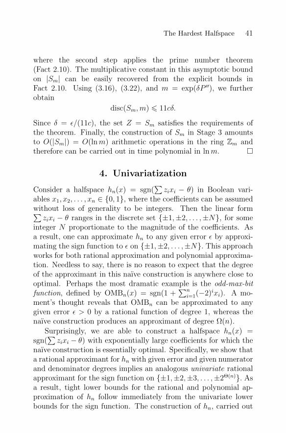
4. Univariatization
Consider a halfspace hn(x) = sgn(∑zixi − θ) in Boolean vari-
ables x1, x2, . . . , xn ∈ 0, 1, where the coefficients can be assumedwithout loss of generality to be integers. Then the linear form∑zixi − θ ranges in the discrete set ±1,±2, . . . ,±N, for some
integer N proportionate to the magnitude of the coefficients. Asa result, one can approximate hn to any given error ε by approxi-mating the sign function to ε on ±1,±2, . . . ,±N. This approachworks for both rational approximation and polynomial approxima-tion. Needless to say, there is no reason to expect that the degreeof the approximant in this naıve construction is anywhere close tooptimal. Perhaps the most dramatic example is the odd-max-bitfunction, defined by OMBn(x) = sgn(1 +
∑ni=1(−2)ixi). A mo-
ment’s thought reveals that OMBn can be approximated to anygiven error ε > 0 by a rational function of degree 1, whereas thenaıve construction produces an approximant of degree Ω(n).
Surprisingly, we are able to construct a halfspace hn(x) =sgn(
∑zixi − θ) with exponentially large coefficients for which the
naıve construction is essentially optimal. Specifically, we show thata rational approximant for hn with given error and given numeratorand denominator degrees implies an analogous univariate rationalapproximant for the sign function on ±1,±2,±3, . . . ,±2Θ(n). Asa result, tight lower bounds for the rational and polynomial ap-proximation of hn follow immediately from the univariate lowerbounds for the sign function. The construction of hn, carried out

42 Alexander A. Sherstov
in this section, is the centerpiece of our paper. The role of hn is toreduce the multivariate problem taken up in this work to a well-understood univariate question, whence the title of this section.We have broken down the proof into four steps, corresponding tosubsections 4.1–4.4 below.
4.1. Distribution of a linear form modulo m . We start bystudying the probability distribution of the weighted sum z1X1 +z2X2 + · · ·+znXn modulo m, where z1, z2, . . . , zn are given integersand X1, X2, . . . , Xn ∈ 0, 1 are chosen uniformly at random. Wewill show that the distribution is close to uniform whenever themultiset z1, z2, . . . , zn has small m-discrepancy. This result usesthe following classical fact on linear forms modulo m.
Fact 4.1 (cf. Gould 1972; Thathachar 1998). Fix a natural num-ber m > 2 and a multiset Z = z1, z2, . . . , zn of integers. Let ωbe a primitive m-th root of unity. Then
(4.2)
∣∣∣∣∣ PX∈0,1n
[n∑j=1
zjXj ≡ s (mod m)
]− 1
m
∣∣∣∣∣6
1
m
m−1∑k=1
∣∣∣∣∣n∏j=1
1 + ωkzj
2
∣∣∣∣∣ , s ∈ Z.
Proof (adapted from Thathachar 1998, Lemma 13). The fractionof vectors X ∈ 0, 1n that satisfy the equation
∑nj=1 zjXj ≡ s
(mod m) can be computed directly, as follows:
PX∈0,1n
[n∑j=1
zjXj ≡ s (mod m)
]
= EX∈0,1n
I
[n∑j=1
zjXj ≡ s (mod m)
]
= EX∈0,1n
1
m
m−1∑k=0
ωk(∑nj=1 zjXj−s)
The Hardest Halfspace 43
= EX∈0,1n
1
m
m−1∑k=0
ω−ksn∏j=1
ωkzjXj
=1
m
m−1∑k=0
ω−ks EX∈0,1n
n∏j=1
ωkzjXj
=1
m
m−1∑k=0
ω−ksn∏j=1
1 + ωkzj
2
=1
m+
1
m
m−1∑k=1
ω−ksn∏j=1
1 + ωkzj
2.
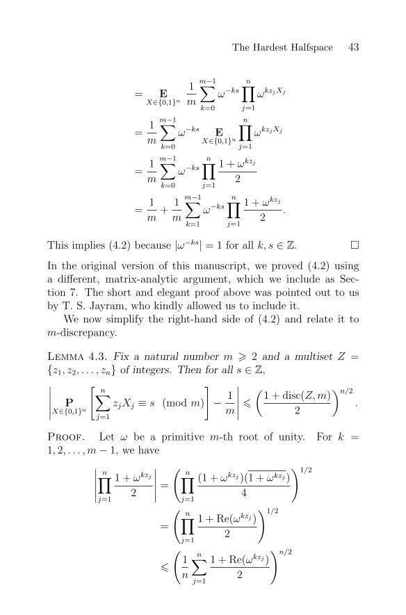
This implies (4.2) because |ω−ks| = 1 for all k, s ∈ Z.
In the original version of this manuscript, we proved (4.2) usinga different, matrix-analytic argument, which we include as Sec-tion 7. The short and elegant proof above was pointed out to usby T. S. Jayram, who kindly allowed us to include it.
We now simplify the right-hand side of (4.2) and relate it tom-discrepancy.
Lemma 4.3. Fix a natural number m > 2 and a multiset Z =z1, z2, . . . , zn of integers. Then for all s ∈ Z,∣∣∣∣∣ PX∈0,1n
[n∑j=1
zjXj ≡ s (mod m)
]− 1
m
∣∣∣∣∣ 6(
1 + disc(Z,m)
2
)n/2.
Proof. Let ω be a primitive m-th root of unity. For k =1, 2, . . . ,m− 1, we have∣∣∣∣∣
n∏j=1
1 + ωkzj
2
∣∣∣∣∣ =
(n∏j=1
(1 + ωkzj)(1 + ωkzj)
4
)1/2
=
(n∏j=1
1 + Re(ωkzj)
2
)1/2
6
(1
n
n∑j=1
1 + Re(ωkzj)
2
)n/2
44 Alexander A. Sherstov
=
(1
2+
1
2Re
(1
n
n∑j=1
ωkzj
))n/2
6
(1
2+
1
2
∣∣∣∣∣ 1nn∑j=1
ωkzj
∣∣∣∣∣)n/2
,
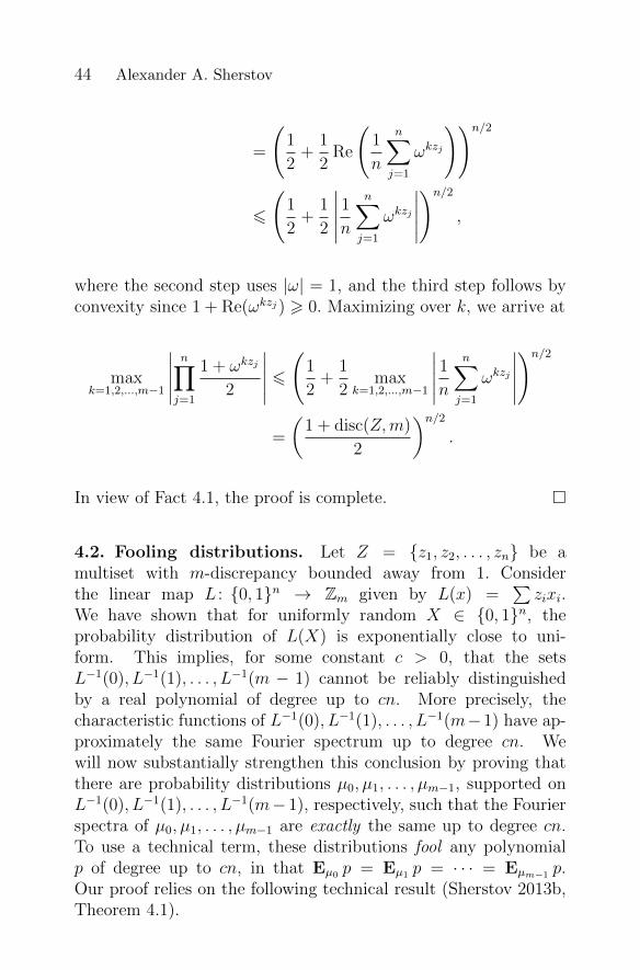
where the second step uses |ω| = 1, and the third step follows byconvexity since 1 + Re(ωkzj) > 0. Maximizing over k, we arrive at
maxk=1,2,...,m−1
∣∣∣∣∣n∏j=1
1 + ωkzj
2
∣∣∣∣∣ 6(
1
2+
1
2max
k=1,2,...,m−1
∣∣∣∣∣ 1nn∑j=1
ωkzj
∣∣∣∣∣)n/2
=
(1 + disc(Z,m)
2
)n/2.
In view of Fact 4.1, the proof is complete.
4.2. Fooling distributions. Let Z = z1, z2, . . . , zn be amultiset with m-discrepancy bounded away from 1. Considerthe linear map L : 0, 1n → Zm given by L(x) =
∑zixi.
We have shown that for uniformly random X ∈ 0, 1n, theprobability distribution of L(X) is exponentially close to uni-form. This implies, for some constant c > 0, that the setsL−1(0), L−1(1), . . . , L−1(m − 1) cannot be reliably distinguishedby a real polynomial of degree up to cn. More precisely, thecharacteristic functions of L−1(0), L−1(1), . . . , L−1(m−1) have ap-proximately the same Fourier spectrum up to degree cn. Wewill now substantially strengthen this conclusion by proving thatthere are probability distributions µ0, µ1, . . . , µm−1, supported onL−1(0), L−1(1), . . . , L−1(m− 1), respectively, such that the Fourierspectra of µ0, µ1, . . . , µm−1 are exactly the same up to degree cn.To use a technical term, these distributions fool any polynomialp of degree up to cn, in that Eµ0 p = Eµ1 p = · · · = Eµm−1 p.Our proof relies on the following technical result (Sherstov 2013b,Theorem 4.1).

The Hardest Halfspace 45
Theorem 4.4 (Sherstov). Let f, χ1, . . . , χk : X → −1,+1 begiven functions on a finite set X . Suppose that
k∑i=1
|〈f, χi〉X | <1
2,(4.5)
k∑j=1j 6=i
|〈χi, χj〉X | 61
2, i = 1, 2, . . . , k.(4.6)
Then there exists a probability distribution µ on X such that
Eµ
[f(x)χi(x)] = 0, i = 1, 2, . . . , k.
By way of notation, we remind the reader that 〈f, g〉X =1|X |∑
x∈X f(x)g(x) for any real-valued functions f and g and anonempty subset X of their domain. In words, Theorem 4.4states that if χ1, χ2, . . . , χk each have small correlation with fand, in addition, have small pairwise correlations, then a distri-bution exists with respect to which f is completely uncorrelatedwith χ1, χ2, . . . , χk. We are now in a position to prove the exis-tence of the promised fooling distributions. In the statement thatfollows, recall that H(p) = −p log p−(1−p) log(1−p) is the binaryentropy function.
Lemma 4.7. Fix δ ∈ [0, 1/2) and a nonempty multiset Z =z1, z2, . . . , zn of integers. Let m be an integer with
(4.8) 2 6 m 6
(2(1− 2δ)
1 + disc(Z,m)
)( 12−δ)n
2−H(δ)n−2.
Define
Xs =
x ∈ 0, 1n :
n∑j=1
zjxj ≡ s (mod m)
, s ∈ Z.(4.9)
Then each Xs is nonempty. Moreover, there is a probability distri-bution µs on Xs (for each s) such that
(4.10) EX∼µs
p(X) = EX∼µs′
p(X)

46 Alexander A. Sherstov
for all s, s′ ∈ Z and all real polynomials p : 0, 1n → R of degreeat most δn.
Proof. For a subset A ⊆ 1, 2, . . . , n, define χA : 0, 1n →−1,+1 by χA(x) = (−1)
∑i∈A xi . The centerpiece of the proof is
the following claim.
Claim 4.11. For every s ∈ Z and every nonempty proper subsetA ⊂ 1, 2, . . . , n,
Xs 6= ∅,(4.12)
|〈χA, 1〉Xs| 6 2m
(1 + disc(Z,m)
2· n
n− |A|
)n−|A|2
.(4.13)
We will proceed with the main proof and settle the claim afterwe are finished. Fix s ∈ Z arbitrarily. Let A denote the family ofnonempty subsets of 1, 2, . . . , n of cardinality at most δn. Recallfrom (2.2) that
(4.14) |A| 6 2H(δ)n − 1.
As a result,∑A∈A
|〈χA, 1〉Xs|
6 |A| · max16|A|6δn
|〈χA, 1〉Xs|
6 (2H(δ)n − 1) · 2m max16k6δn
(1 + disc(Z,m)
2· n
n− k
)n−k2
= (2H(δ)n − 1) · 2m(
1 + disc(Z,m)
2(1− δ)
) (1−δ)n2
<1
2,
(4.15)
where the second step uses (4.14) and Claim 4.11; the third step isvalid because 1 + disc(Z,m) < 2(1− δ) by (4.8); and the final step
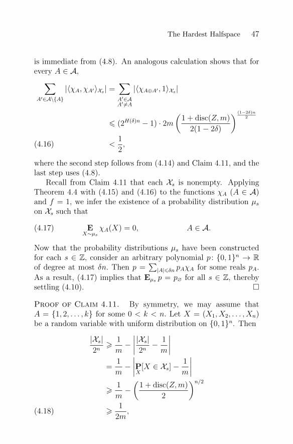
The Hardest Halfspace 47
is immediate from (4.8). An analogous calculation shows that forevery A ∈ A,∑A′∈A\A
|〈χA, χA′〉Xs| =∑A′∈AA′ 6=A
|〈χA⊕A′ , 1〉Xs|
6 (2H(δ)n − 1) · 2m(
1 + disc(Z,m)
2(1− 2δ)
) (1−2δ)n2
<1
2,(4.16)
where the second step follows from (4.14) and Claim 4.11, and thelast step uses (4.8).
Recall from Claim 4.11 that each Xs is nonempty. ApplyingTheorem 4.4 with (4.15) and (4.16) to the functions χA (A ∈ A)and f = 1, we infer the existence of a probability distribution µson Xs such that
EX∼µs
χA(X) = 0, A ∈ A.(4.17)
Now that the probability distributions µs have been constructedfor each s ∈ Z, consider an arbitrary polynomial p : 0, 1n → Rof degree at most δn. Then p =
∑|A|6δn pAχA for some reals pA.
As a result, (4.17) implies that Eµs p = p∅ for all s ∈ Z, therebysettling (4.10).
Proof of Claim 4.11. By symmetry, we may assume thatA = 1, 2, . . . , k for some 0 < k < n. Let X = (X1, X2, . . . , Xn)be a random variable with uniform distribution on 0, 1n. Then
|Xs|2n>
1
m−∣∣∣∣ |Xs|2n
− 1
m
∣∣∣∣=
1
m−∣∣∣∣PX [X ∈ Xs]−
1
m
∣∣∣∣>
1
m−(
1 + disc(Z,m)
2
)n/2>
1
2m,(4.18)
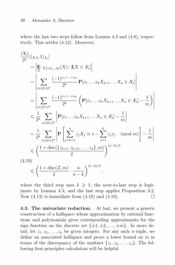
48 Alexander A. Sherstov
where the last two steps follow from Lemma 4.3 and (4.8), respec-tively. This settles (4.12). Moreover,
|Xs|2n|〈χA, 1〉Xs|
=∣∣∣EXχ1,2,...,k(X) · I[X ∈ Xs]
∣∣∣=
∣∣∣∣∣∣∑
x∈0,1k
(−1)x1+···+xk
2kP[x1 . . . xkXk+1 . . . Xn ∈ Xs]
∣∣∣∣∣∣=
∣∣∣∣∣∣∑
x∈0,1k
(−1)x1+···+xk
2k
(P[x1 . . . xkXk+1 . . . Xn ∈ Xs]−
1
m
)∣∣∣∣∣∣6
1
2k
∑x∈0,1k
∣∣∣∣P[x1 . . . xkXk+1 . . . Xn ∈ Xs]−1
m
∣∣∣∣=
1
2k
∑x∈0,1k
∣∣∣∣∣P[
n∑j=k+1
zjXj ≡ s−k∑j=1
zjxj (mod m)
]− 1
m
∣∣∣∣∣6
(1 + disc(zk+1, zk+2, . . . , zn,m)
2
)(n−k)/2
6
(1 + disc(Z,m)
2· n
n− k
)(n−k)/2
,
(4.19)
where the third step uses k > 1; the next-to-last step is legit-imate by Lemma 4.3; and the last step applies Proposition 3.2.Now (4.13) is immediate from (4.18) and (4.19).
4.3. The univariate reduction. At last, we present a genericconstruction of a halfspace whose approximation by rational func-tions and polynomials gives corresponding approximants for thesign function on the discrete set ±1,±2, . . . ,±m. In more de-tail, let z1, z2, . . . , zn be given integers. For any such n-tuple, wedefine an associated halfspace and prove a lower bound on m interms of the discrepancy of the multiset z1, z2, . . . , zn. The fol-lowing first-principles calculation will be helpful.
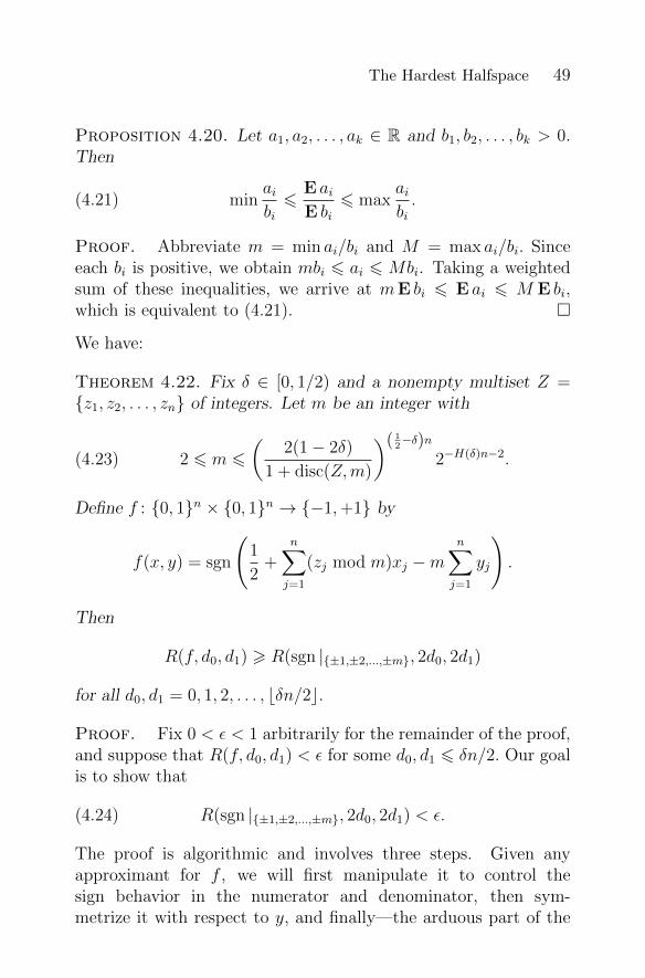
The Hardest Halfspace 49
Proposition 4.20. Let a1, a2, . . . , ak ∈ R and b1, b2, . . . , bk > 0.Then
(4.21) minaibi6
E aiE bi
6 maxaibi.
Proof. Abbreviate m = min ai/bi and M = max ai/bi. Sinceeach bi is positive, we obtain mbi 6 ai 6 Mbi. Taking a weightedsum of these inequalities, we arrive at mE bi 6 E ai 6 M E bi,which is equivalent to (4.21).
We have:
Theorem 4.22. Fix δ ∈ [0, 1/2) and a nonempty multiset Z =z1, z2, . . . , zn of integers. Let m be an integer with
(4.23) 2 6 m 6
(2(1− 2δ)
1 + disc(Z,m)
)( 12−δ)n
2−H(δ)n−2.
Define f : 0, 1n × 0, 1n → −1,+1 by
f(x, y) = sgn
(1
2+
n∑j=1
(zj mod m)xj −mn∑j=1
yj
).
Then
R(f, d0, d1) > R(sgn |±1,±2,...,±m, 2d0, 2d1)
for all d0, d1 = 0, 1, 2, . . . , bδn/2c.
Proof. Fix 0 < ε < 1 arbitrarily for the remainder of the proof,and suppose that R(f, d0, d1) < ε for some d0, d1 6 δn/2. Our goalis to show that
(4.24) R(sgn |±1,±2,...,±m, 2d0, 2d1) < ε.
The proof is algorithmic and involves three steps. Given anyapproximant for f , we will first manipulate it to control thesign behavior in the numerator and denominator, then sym-metrize it with respect to y, and finally—the arduous part of the
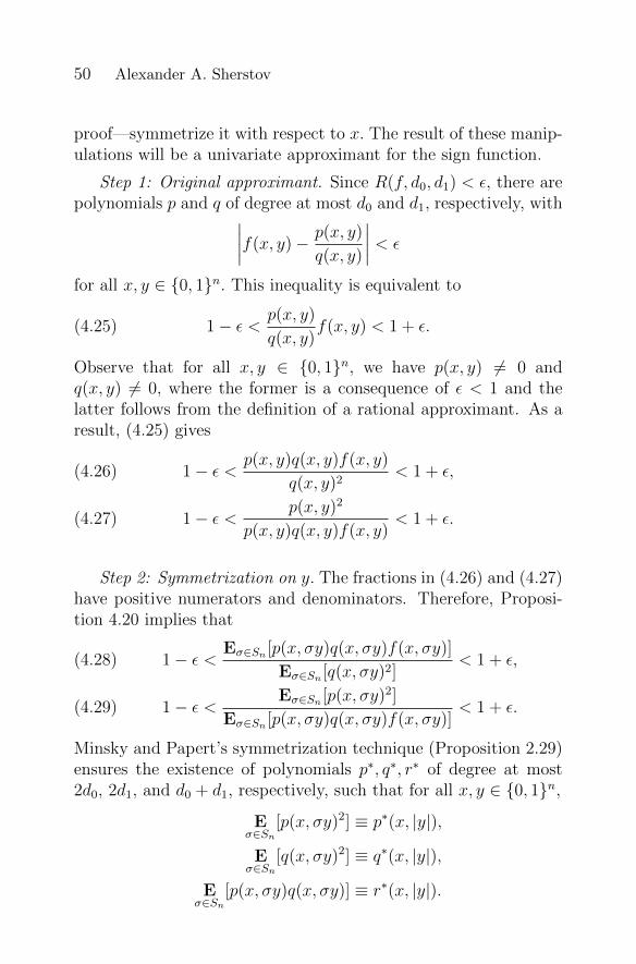
50 Alexander A. Sherstov
proof—symmetrize it with respect to x. The result of these manip-ulations will be a univariate approximant for the sign function.
Step 1: Original approximant. Since R(f, d0, d1) < ε, there arepolynomials p and q of degree at most d0 and d1, respectively, with∣∣∣∣f(x, y)− p(x, y)
q(x, y)
∣∣∣∣ < ε
for all x, y ∈ 0, 1n. This inequality is equivalent to
1− ε < p(x, y)
q(x, y)f(x, y) < 1 + ε.(4.25)
Observe that for all x, y ∈ 0, 1n, we have p(x, y) 6= 0 andq(x, y) 6= 0, where the former is a consequence of ε < 1 and thelatter follows from the definition of a rational approximant. As aresult, (4.25) gives
1− ε < p(x, y)q(x, y)f(x, y)
q(x, y)2< 1 + ε,(4.26)
1− ε < p(x, y)2
p(x, y)q(x, y)f(x, y)< 1 + ε.(4.27)
Step 2: Symmetrization on y. The fractions in (4.26) and (4.27)have positive numerators and denominators. Therefore, Proposi-tion 4.20 implies that
1− ε < Eσ∈Sn [p(x, σy)q(x, σy)f(x, σy)]
Eσ∈Sn [q(x, σy)2]< 1 + ε,(4.28)
1− ε < Eσ∈Sn [p(x, σy)2]
Eσ∈Sn [p(x, σy)q(x, σy)f(x, σy)]< 1 + ε.(4.29)
Minsky and Papert’s symmetrization technique (Proposition 2.29)ensures the existence of polynomials p∗, q∗, r∗ of degree at most2d0, 2d1, and d0 + d1, respectively, such that for all x, y ∈ 0, 1n,
Eσ∈Sn
[p(x, σy)2] ≡ p∗(x, |y|),
Eσ∈Sn
[q(x, σy)2] ≡ q∗(x, |y|),
Eσ∈Sn
[p(x, σy)q(x, σy)] ≡ r∗(x, |y|).
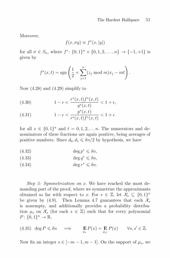
The Hardest Halfspace 51
Moreover,
f(x, σy) ≡ f ∗(x, |y|)
for all σ ∈ Sn, where f ∗ : 0, 1n × 0, 1, 2, . . . , n → −1,+1 isgiven by
f ∗(x, t) = sgn
(1
2+
n∑j=1
(zj mod m)xj −mt
).
Now (4.28) and (4.29) simplify to
1− ε < r∗(x, t)f ∗(x, t)
q∗(x, t)< 1 + ε,(4.30)
1− ε < p∗(x, t)
r∗(x, t)f ∗(x, t)< 1 + ε(4.31)
for all x ∈ 0, 1n and t = 0, 1, 2, . . . n. The numerators and de-nominators of these fractions are again positive, being averages ofpositive numbers. Since d0, d1 6 δn/2 by hypothesis, we have
deg p∗ 6 δn,(4.32)
deg q∗ 6 δn,(4.33)
deg r∗ 6 δn.(4.34)
Step 3: Symmetrization on x. We have reached the most de-manding part of the proof, where we symmetrize the approximantsobtained so far with respect to x. For s ∈ Z, let Xs ⊆ 0, 1nbe given by (4.9). Then Lemma 4.7 guarantees that each Xsis nonempty, and additionally provides a probability distribu-tion µs on Xs (for each s ∈ Z) such that for every polynomialP : 0, 1n → R,
(4.35) degP 6 δn =⇒ EµsP (x) = E
µs′P (x) ∀s, s′ ∈ Z.
Now fix an integer s ∈ [−m− 1,m− 1]. On the support of µs, we
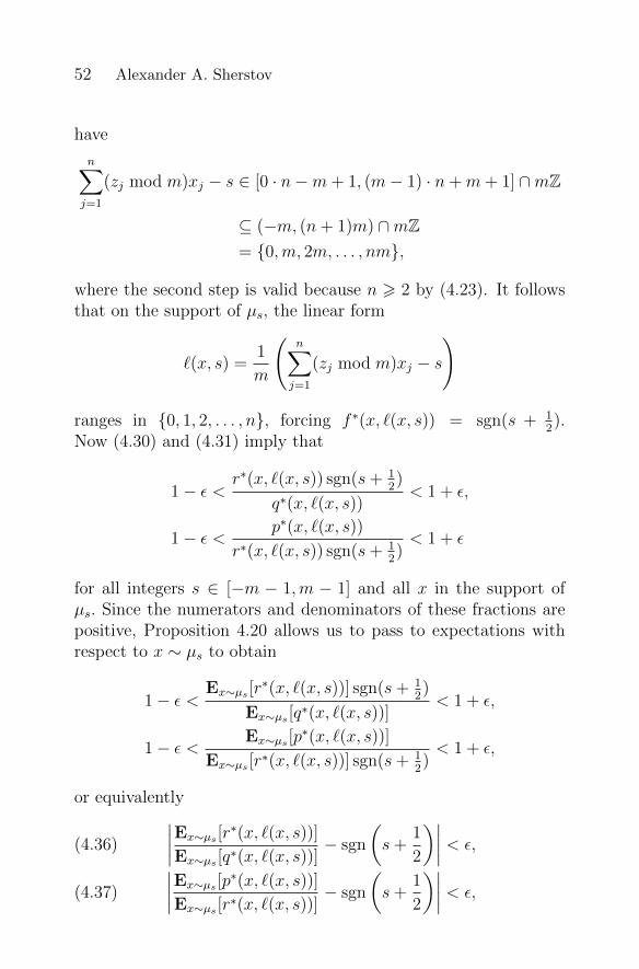
52 Alexander A. Sherstov
have
n∑j=1
(zj mod m)xj − s ∈ [0 · n−m+ 1, (m− 1) · n+m+ 1] ∩mZ
⊆ (−m, (n+ 1)m) ∩mZ= 0,m, 2m, . . . , nm,
where the second step is valid because n > 2 by (4.23). It followsthat on the support of µs, the linear form
`(x, s) =1
m
(n∑j=1
(zj mod m)xj − s
)
ranges in 0, 1, 2, . . . , n, forcing f ∗(x, `(x, s)) = sgn(s + 12).
Now (4.30) and (4.31) imply that
1− ε <r∗(x, `(x, s)) sgn(s+ 1
2)
q∗(x, `(x, s))< 1 + ε,
1− ε < p∗(x, `(x, s))
r∗(x, `(x, s)) sgn(s+ 12)< 1 + ε
for all integers s ∈ [−m − 1,m − 1] and all x in the support ofµs. Since the numerators and denominators of these fractions arepositive, Proposition 4.20 allows us to pass to expectations withrespect to x ∼ µs to obtain
1− ε <Ex∼µs [r
∗(x, `(x, s))] sgn(s+ 12)
Ex∼µs [q∗(x, `(x, s))]
< 1 + ε,
1− ε < Ex∼µs [p∗(x, `(x, s))]
Ex∼µs [r∗(x, `(x, s))] sgn(s+ 1
2)< 1 + ε,
or equivalently∣∣∣∣Ex∼µs [r∗(x, `(x, s))]
Ex∼µs [q∗(x, `(x, s))]
− sgn
(s+
1
2
)∣∣∣∣ < ε,(4.36) ∣∣∣∣Ex∼µs [p∗(x, `(x, s))]
Ex∼µs [r∗(x, `(x, s))]
− sgn
(s+
1
2
)∣∣∣∣ < ε,(4.37)

The Hardest Halfspace 53
for all integers s ∈ [−m− 1,m− 1].Consider the univariate polynomials
p∗∗(s) = Ex∼µs
[p∗(x, `(x, s))],
q∗∗(s) = Ex∼µs
[q∗(x, `(x, s))],
r∗∗(s) = Ex∼µs
[r∗(x, `(x, s))].
Equations (4.36) and (4.37) show that r∗∗(s − 1)/q∗∗(s −1) and p∗∗(s − 1)/r∗∗(s − 1) approximate sgn s pointwise on±1,±2, . . . ,±m to error less than ε. Moreover, (4.32)–(4.35) en-sure that the degrees of p∗∗, q∗∗, r∗∗ are at most the degrees ofp∗, q∗, r∗, respectively. We conclude that
R(sgn |±1,±2,...,±m, d0 + d1, 2d1) < ε,
R(sgn |±1,±2,...,±m, 2d0, d0 + d1) < ε.
These complementary bounds force (4.24) and thereby completethe proof.
4.4. The master theorem. We now combine Theorem 4.22with the efficient construction, in Theorem 3.13, of an integerset with small m-discrepancy for m = 2Θ(n). The result is anexplicit halfspace hn : 0, 1n → −1,+1 whose approximationby polynomials and rational functions is asymptotically equiv-alent to the univariate approximation of the sign function on±1,±2,±3, . . . ,±2Θ(n). We refer to this result as our mastertheorem since all our main theorems are derived from it.
Theorem 4.38. For some constant c′ > 0, there is an algorithmthat takes as input an integer n > 1, runs in time polynomial inn, and outputs a halfspace hn : 0, 1n → −1,+1 with
(4.39) R(hn, d0, d1) > R(
sgn |±1,±2,±3,...,±2bc′nc, 2d0, 2d1
)for all d0, d1 = 0, 1, 2, . . . , bc′nc. Moreover, the constant c′ and thealgorithm are given explicitly.
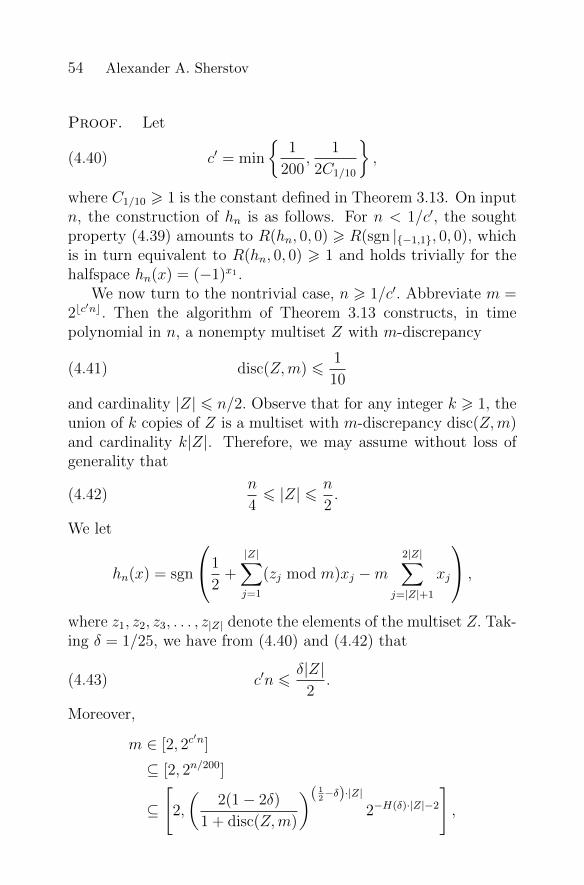
54 Alexander A. Sherstov
Proof. Let
(4.40) c′ = min
1
200,
1
2C1/10
,
where C1/10 > 1 is the constant defined in Theorem 3.13. On inputn, the construction of hn is as follows. For n < 1/c′, the soughtproperty (4.39) amounts to R(hn, 0, 0) > R(sgn |−1,1, 0, 0), whichis in turn equivalent to R(hn, 0, 0) > 1 and holds trivially for thehalfspace hn(x) = (−1)x1 .
We now turn to the nontrivial case, n > 1/c′. Abbreviate m =2bc′nc. Then the algorithm of Theorem 3.13 constructs, in time
polynomial in n, a nonempty multiset Z with m-discrepancy
disc(Z,m) 61
10(4.41)
and cardinality |Z| 6 n/2. Observe that for any integer k > 1, theunion of k copies of Z is a multiset with m-discrepancy disc(Z,m)and cardinality k|Z|. Therefore, we may assume without loss ofgenerality that
(4.42)n
46 |Z| 6 n
2.
We let
hn(x) = sgn
1
2+
|Z|∑j=1
(zj mod m)xj −m2|Z|∑
j=|Z|+1
xj
,
where z1, z2, z3, . . . , z|Z| denote the elements of the multiset Z. Tak-ing δ = 1/25, we have from (4.40) and (4.42) that
(4.43) c′n 6δ|Z|
2.
Moreover,
m ∈ [2, 2c′n]
⊆ [2, 2n/200]
⊆
[2,
(2(1− 2δ)
1 + disc(Z,m)
)( 12−δ)·|Z|
2−H(δ)·|Z|−2
],
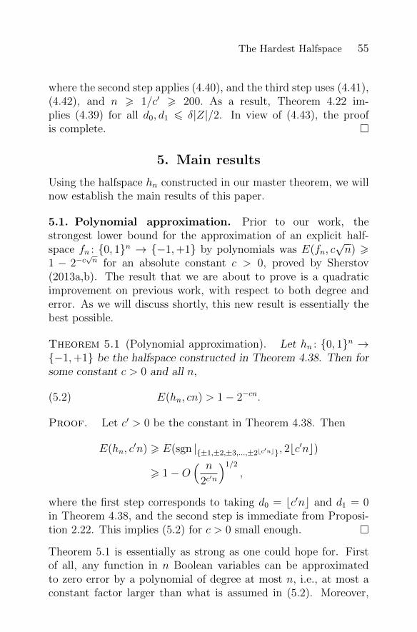
The Hardest Halfspace 55
where the second step applies (4.40), and the third step uses (4.41),(4.42), and n > 1/c′ > 200. As a result, Theorem 4.22 im-plies (4.39) for all d0, d1 6 δ|Z|/2. In view of (4.43), the proofis complete.
5. Main results
Using the halfspace hn constructed in our master theorem, we willnow establish the main results of this paper.
5.1. Polynomial approximation. Prior to our work, thestrongest lower bound for the approximation of an explicit half-space fn : 0, 1n → −1,+1 by polynomials was E(fn, c
√n) >
1 − 2−c√n for an absolute constant c > 0, proved by Sherstov
(2013a,b). The result that we are about to prove is a quadraticimprovement on previous work, with respect to both degree anderror. As we will discuss shortly, this new result is essentially thebest possible.
Theorem 5.1 (Polynomial approximation). Let hn : 0, 1n →−1,+1 be the halfspace constructed in Theorem 4.38. Then forsome constant c > 0 and all n,
(5.2) E(hn, cn) > 1− 2−cn.
Proof. Let c′ > 0 be the constant in Theorem 4.38. Then
E(hn, c′n) > E(sgn |±1,±2,±3,...,±2bc′nc, 2bc
′nc)
> 1−O( n
2c′n
)1/2
,
where the first step corresponds to taking d0 = bc′nc and d1 = 0in Theorem 4.38, and the second step is immediate from Proposi-tion 2.22. This implies (5.2) for c > 0 small enough.
Theorem 5.1 is essentially as strong as one could hope for. Firstof all, any function in n Boolean variables can be approximatedto zero error by a polynomial of degree at most n, i.e., at most aconstant factor larger than what is assumed in (5.2). Moreover,
56 Alexander A. Sherstov
a classic result due to Muroga (1971) implies that for every half-space, the error bound in (5.2) is almost achieved by polynomialsof degree 1:
Fact 5.3. There is an absolute constant c > 0 such that for everyn and every halfspace h : 0, 1n → −1,+1,
E(h, 1) 6 1− n−cn.
Proof. Muroga (1971) showed that every halfspaceh : 0, 1n → −1,+1 can be represented as h(x) =sgn(
∑nj=1 zjxj − θ) for some integers z1, z2, . . . , zn, θ whose
absolute values sum to nO(n). It follows that
E(h, 1) 6 maxx∈0,1n
∣∣∣∣∣h(x)− 1
|θ|+∑n
j=1 |zj|
(n∑j=1
zjxj − θ
)∣∣∣∣∣6 1− 1
|θ|+∑n
j=1 |zj|6 1− n−O(n).
5.2. Rational approximation. We now show that the half-space hn constructed in our master theorem cannot be approxi-mated pointwise to any small constant except by rational functionsof degree Ω(n). This degree lower bound matches the trivial up-per bound and is a quadratic improvement on the previous bestconstruction (Sherstov 2013a,b). More generally, we derive a lowerbound on the approximation of hn by rational functions of anygiven degree d, and this lower bound too is essentially the bestpossible for any halfspace. Details follow.
Theorem 5.4 (Rational approximation). Let hn : 0, 1n →−1,+1 be the halfspace constructed in Theorem 4.38. Then forsome constant c > 0 and all n,
R(hn, d) > 1− exp(−cnd
), d = 1, 2, . . . , bcnc.(5.5)
The Hardest Halfspace 57
Proof. Let c′ > 0 be the constant in Theorem 4.38. Then ford = 1, 2, . . . , bc′nc, we have
R(hn, d) > R(sgn |±1,±2,±3,...,±2bc′nc, 2d)
> 1− exp(−Θ
(nd
)),
where the first step corresponds to taking d0 = d1 = d in Theo-rem 4.38, and the second step is immediate from Theorem 2.25.This implies (5.5) for c > 0 small enough.
We now show that the lower bounds on the approximation error inTheorem 5.4 are essentially the best possible for any halfspace.
Fact 5.6. There exists an absolute constant c > 0 such that forevery n and every halfspace h : 0, 1n → −1,+1,
R(h, d) 6 1− exp
(−cn log n
d
), d = 1, 2, . . . , n.
Proof. As already mentioned, Muroga (1971) showed thath(x) ≡ sgn p(x) for some linear polynomial p(x) that ranges in[−N,−1]∪ [1, N ], where N = exp(cn log n) for some absolute con-stant c > 0. This makes it possible to obtain a rational approx-imant for h(x) by taking any rational approximant for the signfunction on [−N,−1] ∪ [1, N ] and composing it with p(x). Weconclude that for any integer d,
R(h, d) 6 R(sgn |[−N,−1]∪[1,N ], d)
6 1− 1
N1/d
= 1− exp
(−cn log n
d
),
where the second step uses Newman’s rational approximation(Fact 2.24).
5.3. Threshold degree. Here, we use the halfspace hn con-structed in our master theorem to study the degree required tosign-represent intersections of halfspaces. Our result is a lower
58 Alexander A. Sherstov
bound of Ω(n) for the intersection hn ∧ hn of two independentcopies of hn. This result improves quadratically on the previousbest construction (Sherstov 2013a,b) and matches the trivial up-per bound of O(n) for sign-representing any Boolean function in nvariables.
Theorem 5.7. Let hn : 0, 1n → −1,+1 be the halfspace con-structed in Theorem 4.38. Then
deg±(hn ∧ hn) = Ω(n).
Proof. Abbreviate Dn = deg±(hn ∧ hn). Taking f = g = hn inTheorem 2.28 shows that R(hn, 4Dn) < 1/2, which by Theorem 5.4forces Dn = Ω(n).
Theorem 5.7 should be contrasted with the result of Beigel et al.(1995) that the conjunction of any constant number of majorityfunctions on 0, 1n has threshold degree O(log n). We now derivea lower bound of Ω(
√n log n) on the threshold degree of the inter-
section of an explicitly given halfspace and a majority function, im-proving quadratically on the previous best construction (Sherstov2013a,b). As we discuss shortly, the new construction is optimalup to a logarithmic factor.
Theorem 5.8. Let hn : 0, 1n → −1,+1 be the halfspace con-structed in Theorem 4.38. Then
deg±(hn ∧MAJn) = Ω(√n log n).(5.9)
Proof. Abbreviate Dn = deg±(hn∧MAJn). Then R(hn, 4Dn)+R(MAJn, 2Dn) < 1 by Theorem 2.28. The lower bounds for therational approximation of hn and MAJn in Theorem 2.26 and The-orem 5.4 now imply that Dn = Ω(
√n log n).
Remark 5.10. The construction of Theorem 5.8 is essentially thebest possible, in that
(5.11) deg±(h ∧MAJn) = O(√n log n)
for every halfspace h : 0, 1n → −1,+1. Indeed, taking d =C√n log n in Theorem 2.26 and Fact 5.6 for a large enough con-
stant C > 1 yields R(h,C√n log n) + R(MAJn, C
√n log n) < 1,
which in turn implies (5.11) in view of Theorem 2.27.
The Hardest Halfspace 59
5.4. Threshold density. In addition to threshold degree,several other complexity measures are of interest when sign-representing Boolean functions by real polynomials. One suchcomplexity measure is threshold density, defined as the least k forwhich a given function can be sign-represented by a linear com-bination of k parity functions. Formally, for a given functionf : 0, 1n → −1,+1, its threshold density dns(f) is the min-imum size |S| of a family S ⊆ P(1, 2, . . . , n) such that
f(x) ≡ sgn
(∑S∈S
wS(−1)∑j∈S xj
)
for some reals wS. It is clear from the definition that dns(f) 6 2n
for all functions f : 0, 1n → −1,+1, and we will now con-struct a pair of halfspaces whose intersection has threshold density2Θ(n). Prior to our work, the best construction (Sherstov 2013a)had threshold density 2Θ(
√n).
To proceed, we recall a technique due to Krause & Pudlak(1997) that transforms Boolean functions with high threshold de-gree into Boolean functions with high threshold density. Theirtransformation works in a black-box manner and sends a func-tion f : 0, 1n → −1,+1 to the function fKP : (0, 1n)3 →−1,+1 defined by
fKP(x, y, z) = f(. . . , (zi ∧ xi) ∨ (zi ∧ yi), . . . ).
The threshold degree of f and the threshold density of fKP arerelated as follows (Krause & Pudlak 1997, Proposition 2.1).
Theorem 5.12 (Krause and Pudlak). For every functionf : 0, 1n → −1,+1,
dns(fKP) > 2deg±(f).
We are now in a position to obtain the claimed density results.
Theorem 5.13. There is an (explicit) algorithm that takes as in-put an integer n > 1, runs in time polynomial in n, and outputs a
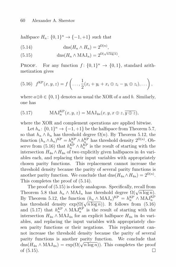
60 Alexander A. Sherstov
halfspace Hn : 0, 1n → −1,+1 such that
dns(Hn ∧Hn) = 2Ω(n),(5.14)
dns(Hn ∧MAJn) = 2Ω(√n logn).(5.15)
Proof. For any function f : 0, 1n → 0, 1, standard arith-metization gives
(5.16) fKP(x, y, z) = f
(. . . ,
1
2(xi + yi + xi ⊕ zi − yi ⊕ zi), . . .
),
where a⊕b ∈ 0, 1 denotes as usual the XOR of a and b. Similarly,one has
(5.17) MAJKPn (x, y, z) = MAJ4n(x, y, x⊕ z, y ⊕ z),
where the XOR and complement operations are applied bitwise.Let hn : 0, 1n → −1,+1 be the halfspace from Theorem 5.7,
so that hn ∧ hn has threshold degree Ω(n). By Theorem 5.12, thefunction (hn ∧ hn)KP = hKP
n ∧ hKPn has threshold density 2Ω(n). Ob-
serve from (5.16) that hKPn ∧ hKP
n is the result of starting with theintersection H4n∧H4n of two explicitly given halfspaces in 4n vari-ables each, and replacing their input variables with appropriatelychosen parity functions. This replacement cannot increase thethreshold density because the parity of several parity functions isanother parity function. We conclude that dns(H4n∧H4n) = 2Ω(n).This completes the proof of (5.14).
The proof of (5.15) is closely analogous. Specifically, recall fromTheorem 5.8 that hn ∧ MAJn has threshold degree Ω(
√n log n).
By Theorem 5.12, the function (hn ∧ MAJn)KP = hKPn ∧ MAJKP
n
has threshold density exp(Ω(√n log n)). It follows from (5.16)
and (5.17) that hKPn ∧ MAJKP
n is the result of starting with theintersection H4n ∧MAJ4n for an explicit halfspace H4n in 4n vari-ables, and replacing the input variables with appropriately cho-sen parity functions or their negations. This replacement can-not increase the threshold density because the parity of severalparity functions is another parity function. We conclude thatdns(H4n ∧MAJ4n) = exp(Ω(
√n log n)). This completes the proof
of (5.15).
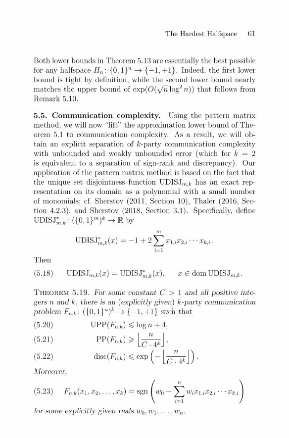
The Hardest Halfspace 61
Both lower bounds in Theorem 5.13 are essentially the best possiblefor any halfspace Hn : 0, 1n → −1,+1. Indeed, the first lowerbound is tight by definition, while the second lower bound nearlymatches the upper bound of exp(O(
√n log2 n)) that follows from
Remark 5.10.
5.5. Communication complexity. Using the pattern matrixmethod, we will now “lift” the approximation lower bound of The-orem 5.1 to communication complexity. As a result, we will ob-tain an explicit separation of k-party communication complexitywith unbounded and weakly unbounded error (which for k = 2is equivalent to a separation of sign-rank and discrepancy). Ourapplication of the pattern matrix method is based on the fact thatthe unique set disjointness function UDISJm,k has an exact rep-resentation on its domain as a polynomial with a small numberof monomials; cf. Sherstov (2011, Section 10), Thaler (2016, Sec-tion 4.2.3), and Sherstov (2018, Section 3.1). Specifically, defineUDISJ∗m,k : (0, 1m)k → R by
UDISJ∗m,k(x) = −1 + 2m∑i=1
x1,ix2,i · · ·xk,i .
Then
UDISJm,k(x) = UDISJ∗m,k(x), x ∈ dom UDISJm,k.(5.18)
Theorem 5.19. For some constant C > 1 and all positive inte-gers n and k, there is an (explicitly given) k-party communicationproblem Fn,k : (0, 1n)k → −1,+1 such that
UPP(Fn,k) 6 log n+ 4,(5.20)
PP(Fn,k) >⌊ n
C · 4k⌋,(5.21)
disc(Fn,k) 6 exp(−⌊ n
C · 4k⌋)
.(5.22)
Moreover,
Fn,k(x1, x2, . . . , xk) = sgn
(w0 +
n∑i=1
wix1,ix2,i · · ·xk,i
)(5.23)
for some explicitly given reals w0, w1, . . . , wn.
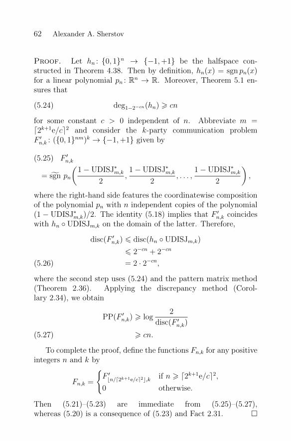
62 Alexander A. Sherstov
Proof. Let hn : 0, 1n → −1,+1 be the halfspace con-structed in Theorem 4.38. Then by definition, hn(x) = sgn pn(x)for a linear polynomial pn : Rn → R. Moreover, Theorem 5.1 en-sures that
deg1−2−cn(hn) > cn(5.24)
for some constant c > 0 independent of n. Abbreviate m =d2k+1e/ce2 and consider the k-party communication problemF ′n,k : (0, 1nm)k → −1,+1 given by
(5.25) F ′n,k
= sgn pn
(1− UDISJ∗m,k
2,1− UDISJ∗m,k
2, . . . ,
1− UDISJ∗m,k2
),
where the right-hand side features the coordinatewise compositionof the polynomial pn with n independent copies of the polynomial(1 − UDISJ∗m,k)/2. The identity (5.18) implies that F ′n,k coincideswith hn UDISJm,k on the domain of the latter. Therefore,
disc(F ′n,k) 6 disc(hn UDISJm,k)
6 2−cn + 2−cn
= 2 · 2−cn,(5.26)
where the second step uses (5.24) and the pattern matrix method(Theorem 2.36). Applying the discrepancy method (Corol-lary 2.34), we obtain
PP(F ′n,k) > log2
disc(F ′n,k)
> cn.(5.27)
To complete the proof, define the functions Fn,k for any positiveintegers n and k by
Fn,k =
F ′bn/d2k+1e/ce2c,k if n > d2k+1e/ce2,0 otherwise.
Then (5.21)–(5.23) are immediate from (5.25)–(5.27),whereas (5.20) is a consequence of (5.23) and Fact 2.31.
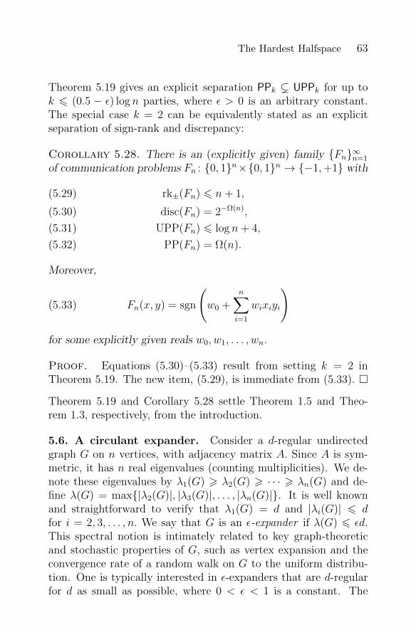
The Hardest Halfspace 63
Theorem 5.19 gives an explicit separation PPk ( UPPk for up tok 6 (0.5 − ε) log n parties, where ε > 0 is an arbitrary constant.The special case k = 2 can be equivalently stated as an explicitseparation of sign-rank and discrepancy:
Corollary 5.28. There is an (explicitly given) family Fn∞n=1
of communication problems Fn : 0, 1n×0, 1n → −1,+1 with
rk±(Fn) 6 n+ 1,(5.29)
disc(Fn) = 2−Ω(n),(5.30)
UPP(Fn) 6 log n+ 4,(5.31)
PP(Fn) = Ω(n).(5.32)
Moreover,
Fn(x, y) = sgn
(w0 +
n∑i=1
wixiyi
)(5.33)
for some explicitly given reals w0, w1, . . . , wn.
Proof. Equations (5.30)–(5.33) result from setting k = 2 inTheorem 5.19. The new item, (5.29), is immediate from (5.33).
Theorem 5.19 and Corollary 5.28 settle Theorem 1.5 and Theo-rem 1.3, respectively, from the introduction.
5.6. A circulant expander. Consider a d-regular undirectedgraph G on n vertices, with adjacency matrix A. Since A is sym-metric, it has n real eigenvalues (counting multiplicities). We de-note these eigenvalues by λ1(G) > λ2(G) > · · · > λn(G) and de-fine λ(G) = max|λ2(G)|, |λ3(G)|, . . . , |λn(G)|. It is well knownand straightforward to verify that λ1(G) = d and |λi(G)| 6 dfor i = 2, 3, . . . , n. We say that G is an ε-expander if λ(G) 6 εd.This spectral notion is intimately related to key graph-theoreticand stochastic properties of G, such as vertex expansion and theconvergence rate of a random walk on G to the uniform distribu-tion. One is typically interested in ε-expanders that are d-regularfor d as small as possible, where 0 < ε < 1 is a constant. The
64 Alexander A. Sherstov
existence of expanders with strong parameters can be verified us-ing the probabilistic method (Alon & Spencer 2008), and explicitconstructions are known as well.
In this section, we study the problem of constructing circulantexpanders. Formally, a graph is circulant if its adjacency ma-trix is circulant. It is clear that a circulant graph is d-regular forsome d, meaning that every vertex has out-degree d and in-degreed. We focus on circulant graphs that are undirected and have noself-loops, which corresponds to adjacency matrices that are sym-metric and have zeroes on the diagonal. It is well known (Alon &Roichman 1994) that for any 0 < ε < 1 and all large enough n,there exists a circulant ε-expander on n vertices of degree O(log n).This degree bound is asymptotically optimal (Alon & Roichman1994; Friedman et al. 2006; Leung et al. 2011), and the problem ofconstructing such circulant expanders explicitly has been studiedby several authors (Alon 1986; Ajtai et al. 1990; Alon & Roich-man 1994). The best construction prior to our work, due to Ajtaiet al. (1990), achieves degree (log∗ n)O(log∗ n) log n. In this section,we construct a circulant ε-expander of optimal degree, O(log n),for any constant 0 < ε < 1. By way of terminology, recall thatthe adjacency matrix of a circulant graph on n vertices is circ(1S)for some subset S ⊆ 0, 1, 2, . . . , n − 1. With this in mind, wesay that an algorithm constructs a circulant graph on n vertices intime T (n) if the algorithm outputs in time T (n) the elements of theassociated subset S. The formal statement of our result follows.
Theorem 5.34. Let 0 < ε < 1 be given. Then there is an(explicitly given) algorithm that takes as input an integer n > 2and constructs in time polynomial in log n an undirected simpled-regular circulant graph Gn on n vertices, where
1 6 d 6 O(log n),(5.35)
λ(Gn) 6 max
ε,
1
n− 1
d.(5.36)
Proof. Let Cε be the constant from Theorem 3.13. We firstconsider the trivial case when 2(Cε log n)2 > n, which means thatn is bounded by an explicit constant. In this case, we take Gn
The Hardest Halfspace 65
to be the complete graph on n vertices. It is clear that Gn is ad-regular circulant graph for d = n − 1. The adjacency matrix ofGn is circ(0, 1, 1, . . . , 1), whose eigenvalues by Corollary 2.17 aren− 1,−1,−1, . . . ,−1. In particular, λ(Gn) = 1 = d/(n− 1). Thissettles (5.36), whereas (5.35) holds trivially because d and n arebounded by a constant.
We now turn to the nontrivial case when 2(Cε log n)2 < n. Thealgorithm of Theorem 3.13 constructs, in time polynomial in log n,a set Z ⊆ 0, 1, 2, . . . , n− 1 with
disc(Z, n) 6 ε,(5.37)
1 6 |Z| 6 Cε log n.(5.38)
For any z, z′ ∈ Z, the linear congruence z+∆ ≡ −(z′+∆) (mod n)has at most two solutions ∆ ∈ 0, 1, 2, . . . , n − 1. Recalling that2|Z|2 < n in the case under consideration, we conclude that thereexists ∆ ∈ 0, 1, 2, . . . , 2|Z|2 with
(5.39) z + ∆ 6≡ −(z′ + ∆) (mod n), z, z′ ∈ Z.
Moreover, such ∆ can clearly be found by brute force search in timepolynomial in |Z| = O(log n). Equation (5.39) now implies that notwo elements of the multiset (Z + ∆) ∪ (−Z − ∆) are congruentmodulo n, and in particular no element of Z + ∆ is congruent to 0modulo n.
We define Gn to be the undirected graph with vertex set0, 1, 2, . . . , n − 1 in which (i, j) is an edge if and only if i − jis congruent modulo n to an element of (Z + ∆)∪ (−Z −∆). Theroles of i and j in this definition are symmetric, making Gn anundirected graph. It is obvious that the adjacency matrix of Gn iscirculant. Furthermore, Gn has no self-loops because by construc-tion no element of Z + ∆ is congruent to 0 modulo n. Since theelements of (Z+∆)∪(−Z−∆) are pairwise distinct modulo n, thedegree of Gn is |(Z + ∆) ∪ (−Z −∆)| = 2|Z|. Now (5.35) followsfrom (5.38). To settle the remaining property (5.36), observe thatthe first row of the adjacency matrix of Gn is the characteristicvector of the set ((Z + ∆)∪ (−Z −∆)) mod n. As a result, Corol-lary 2.17 implies that the eigenvalues of the adjacency matrix of
66 Alexander A. Sherstov
Gn are ∑z∈Z+∆
ωkz +∑
z∈−Z−∆
ωkz, k = 0, 1, 2, . . . , n− 1,
where ω is a primitive n-th root of unity. Setting k = 0 yields thelargest eigenvalue, 2|Z|. The other eigenvalues are bounded by
λ(Gn) = maxk=1,2,...,n−1
∣∣∣∣∣ ∑z∈Z+∆
ωkz +∑
z∈−Z−∆
ωkz
∣∣∣∣∣6 max
k=1,2,...,n−1
∣∣∣∣∣ ∑z∈Z+∆
ωkz
∣∣∣∣∣+ maxk=1,2,...,n−1
∣∣∣∣∣ ∑z∈−Z−∆
ωkz
∣∣∣∣∣= 2|Z| disc(Z, n).
Along with (5.37), this proves (5.36).
6. The iteration lemma of Ajtai et al.
The purpose of this section is to provide a detailed and self-contained proof of Theorem 3.12, which we restate below for thereader’s convenience.
Theorem. Fix an integer R > 1 and a real number P > 2. Letm be an integer with
m > P 2(R + 1).
Fix a set Sp ⊆ 1, 2, . . . , p − 1 for each prime p ∈ (P/2, P ] withp - m, such that all Sp have the same cardinality. Consider themultiset
S = (r + s · (p−1)m) mod m :
r = 1, . . . , R; p ∈ (P/2, P ] prime with p - m; s ∈ Sp.
Then the elements of S are pairwise distinct and nonzero. More-over,
(6.1) disc(S,m) 6c√R
+c logm
log logm· logP
P+ max
pdisc(Sp, p)
for some (explicitly given) constant c > 1 independent of P,R,m.
The Hardest Halfspace 67
This result is a slight generalization of the iteration lemma of Ajtaiet al. (1990), which corresponds to the special case for m prime.We closely follow their proof but provide ample detail to make itmore accessible. We have structured the presentation around fivekey milestones, corresponding to Section 6.1–Section 6.5 below.Before proceeding, the reader may wish to review the number-theoretic preliminaries in Section 2.2.
6.1. Shorthand notation. In the remainder of this manuscript,we adopt the shorthand
e(x) = exp(2πxi),
where i is the imaginary unit. We will need the following bounds,illustrated in Figure 6.1:
|1− e(x)| 6 2πx, 0 6 x 6 1,(6.2)
|1− e(x)| > 4 min(x, 1− x), 0 6 x 6 1.(6.3)
To verify these bounds, write |1 − e(x)| = |1 − exp(2πxi)| =√2− 2 cos(2πx) and apply elementary calculus.We let P denote the set of prime numbers p ∈ (P/2, P ] with
p - m. In this notation, the multiset S is given by
S = (r + s · (p−1)m) mod m : p ∈ P , s ∈ Sp, r = 1, 2, . . . , R.
There are precisely π(P )− π(P/2) primes in (P/2, P ], of which atmost ν(m) are prime divisors of m. Therefore,
(6.4) |P| > π(P )− π(P
2
)− ν(m).
6.2. Elements of S are nonzero and distinct. As our firststep, we verify that the elements of S are nonzero modulo m. Con-sider any r ∈ 1, 2, . . . , R, any prime p ∈ (P/2, P ] with p - m, andany s ∈ Sp. Then pr+s ∈ [1, PR+P−1] ⊆ [1,m). This means thatpr+ s 6≡ 0 (mod m), which in turn implies that r+ s · (p−1)m 6≡ 0(mod m).
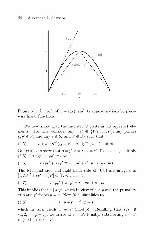
68 Alexander A. Sherstov
Figure 6.1: A graph of |1− e(x)| and its approximations by piece-wise linear functions.
We now show that the multiset S contains no repeated ele-ments. For this, consider any r, r′ ∈ 1, 2, . . . , R, any primesp, p′ ∈ P , and any s ∈ Sp and s′ ∈ Sp′ such that
(6.5) r + s · (p−1)m ≡ r′ + s′ · (p′−1)m (mod m).
Our goal is to show that p = p′, r = r′, s = s′. To this end, multiply(6.5) through by pp′ to obtain
(6.6) r · pp′ + s · p′ ≡ r′ · pp′ + s′ · p (mod m).
The left-hand side and right-hand side of (6.6) are integers in[1, RP 2 + (P − 1)P ] ⊆ [1,m), whence
(6.7) r · pp′ + s · p′ = r′ · pp′ + s′ · p.
This implies that p | s ·p′, which in view of s < p and the primalityof p and p′ forces p = p′. Now (6.7) simplifies to
(6.8) r · p+ s = r′ · p+ s′,
which in turn yields s ≡ s′ (mod p). Recalling that s, s′ ∈1, 2, . . . , p − 1, we arrive at s = s′. Finally, substituting s = s′
in (6.8) gives r = r′.
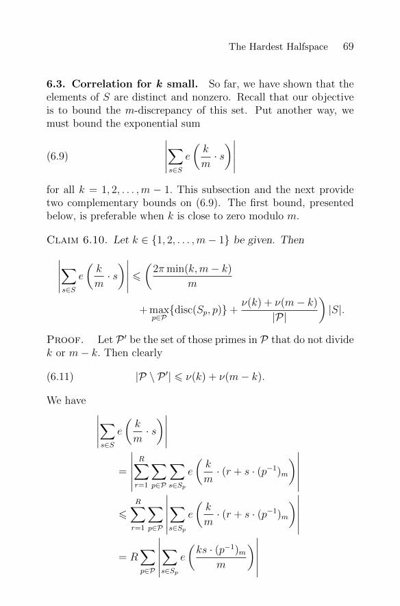
The Hardest Halfspace 69
6.3. Correlation for k small. So far, we have shown that theelements of S are distinct and nonzero. Recall that our objectiveis to bound the m-discrepancy of this set. Put another way, wemust bound the exponential sum
(6.9)
∣∣∣∣∣∑s∈S
e
(k
m· s)∣∣∣∣∣
for all k = 1, 2, . . . ,m − 1. This subsection and the next providetwo complementary bounds on (6.9). The first bound, presentedbelow, is preferable when k is close to zero modulo m.
Claim 6.10. Let k ∈ 1, 2, . . . ,m− 1 be given. Then∣∣∣∣∣∑s∈S
e
(k
m· s)∣∣∣∣∣ 6
(2πmin(k,m− k)
m
+ maxp∈Pdisc(Sp, p)+
ν(k) + ν(m− k)
|P|
)|S|.
Proof. Let P ′ be the set of those primes in P that do not dividek or m− k. Then clearly
(6.11) |P \ P ′| 6 ν(k) + ν(m− k).
We have ∣∣∣∣∣∑s∈S
e
(k
m· s)∣∣∣∣∣
=
∣∣∣∣∣∣R∑r=1
∑p∈P
∑s∈Sp
e
(k
m· (r + s · (p−1)m
)∣∣∣∣∣∣6
R∑r=1
∑p∈P
∣∣∣∣∣∣∑s∈Sp
e
(k
m· (r + s · (p−1)m
)∣∣∣∣∣∣= R
∑p∈P
∣∣∣∣∣∣∑s∈Sp
e
(ks · (p−1)m
m
)∣∣∣∣∣∣
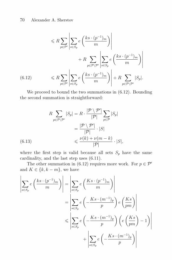
70 Alexander A. Sherstov
6 R∑p∈P ′
∣∣∣∣∣∣∑s∈Sp
e
(ks · (p−1)m
m
)∣∣∣∣∣∣+R
∑p∈P\P ′
∣∣∣∣∣∣∑s∈Sp
e
(ks · (p−1)m
m
)∣∣∣∣∣∣6 R
∑p∈P ′
∣∣∣∣∣∣∑s∈Sp
e
(ks · (p−1)m
m
)∣∣∣∣∣∣+R∑
p∈P\P ′|Sp|.(6.12)
We proceed to bound the two summations in (6.12). Boundingthe second summation is straightforward:
R∑
p∈P\P ′|Sp| = R · |P \ P
′||P|
∑p∈P
|Sp|
=|P \ P ′||P|
· |S|
6ν(k) + ν(m− k)
|P|· |S|,(6.13)
where the first step is valid because all sets Sp have the samecardinality, and the last step uses (6.11).
The other summation in (6.12) requires more work. For p ∈ P ′and K ∈ k, k −m, we have∣∣∣∣∣∣∑s∈Sp
e
(ks · (p−1)m
m
)∣∣∣∣∣∣ =
∣∣∣∣∣∣∑s∈Sp
e
(Ks · (p−1)m
m
)∣∣∣∣∣∣=
∣∣∣∣∣∣∑s∈Sp
e
(−Ks · (m
−1)pp
)e
(Ks
pm
)∣∣∣∣∣∣6
∣∣∣∣∣∣∑s∈Sp
e
(−Ks · (m
−1)pp
)(e
(Ks
pm
)− 1
)∣∣∣∣∣∣+
∣∣∣∣∣∣∑s∈Sp
e
(−Ks · (m
−1)pp
)∣∣∣∣∣∣
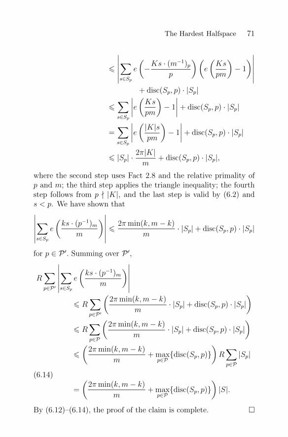
The Hardest Halfspace 71
6
∣∣∣∣∣∣∑s∈Sp
e
(−Ks · (m
−1)pp
)(e
(Ks
pm
)− 1
)∣∣∣∣∣∣+ disc(Sp, p) · |Sp|
6∑s∈Sp
∣∣∣∣e(Kspm)− 1
∣∣∣∣+ disc(Sp, p) · |Sp|
=∑s∈Sp
∣∣∣∣e( |K|spm
)− 1
∣∣∣∣+ disc(Sp, p) · |Sp|
6 |Sp| ·2π|K|m
+ disc(Sp, p) · |Sp|,
where the second step uses Fact 2.8 and the relative primality ofp and m; the third step applies the triangle inequality; the fourthstep follows from p - |K|, and the last step is valid by (6.2) ands < p. We have shown that∣∣∣∣∣∣∑s∈Sp
e
(ks · (p−1)m
m
)∣∣∣∣∣∣ 6 2πmin(k,m− k)
m· |Sp|+ disc(Sp, p) · |Sp|
for p ∈ P ′. Summing over P ′,
R∑p∈P ′
∣∣∣∣∣∣∑s∈Sp
e
(ks · (p−1)m
m
)∣∣∣∣∣∣6 R
∑p∈P ′
(2πmin(k,m− k)
m· |Sp|+ disc(Sp, p) · |Sp|
)6 R
∑p∈P
(2πmin(k,m− k)
m· |Sp|+ disc(Sp, p) · |Sp|
)6
(2πmin(k,m− k)
m+ max
p∈Pdisc(Sp, p)
)R∑p∈P
|Sp|
=
(2πmin(k,m− k)
m+ max
p∈Pdisc(Sp, p)
)|S|.
(6.14)
By (6.12)–(6.14), the proof of the claim is complete.
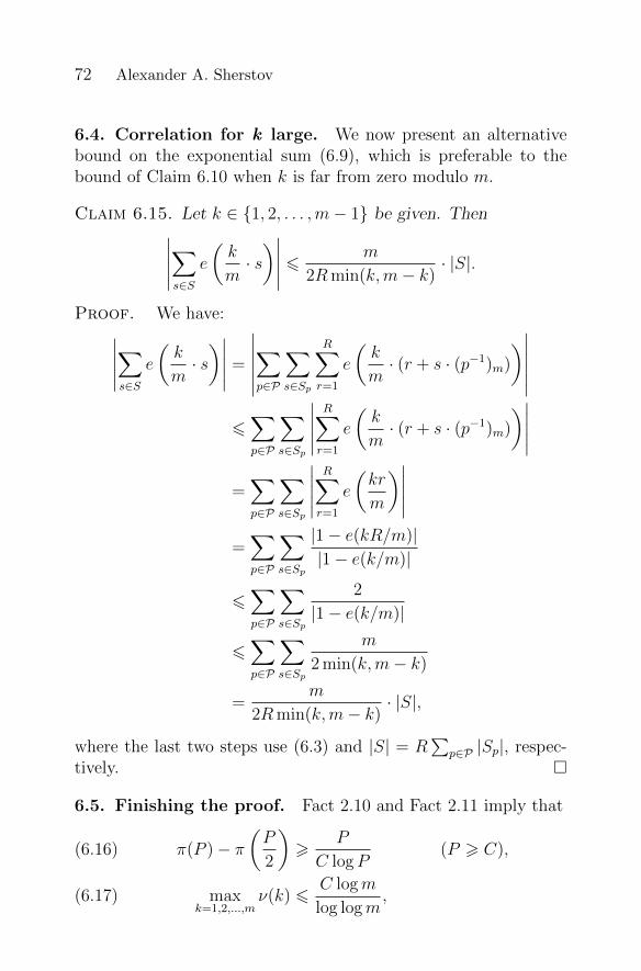
72 Alexander A. Sherstov
6.4. Correlation for k large. We now present an alternativebound on the exponential sum (6.9), which is preferable to thebound of Claim 6.10 when k is far from zero modulo m.
Claim 6.15. Let k ∈ 1, 2, . . . ,m− 1 be given. Then∣∣∣∣∣∑s∈S
e
(k
m· s)∣∣∣∣∣ 6 m
2Rmin(k,m− k)· |S|.
Proof. We have:∣∣∣∣∣∑s∈S
e
(k
m· s)∣∣∣∣∣ =
∣∣∣∣∣∣∑p∈P
∑s∈Sp
R∑r=1
e
(k
m· (r + s · (p−1)m)
)∣∣∣∣∣∣6∑p∈P
∑s∈Sp
∣∣∣∣∣R∑r=1
e
(k
m· (r + s · (p−1)m)
)∣∣∣∣∣=∑p∈P
∑s∈Sp
∣∣∣∣∣R∑r=1
e
(kr
m
)∣∣∣∣∣=∑p∈P
∑s∈Sp
|1− e(kR/m)||1− e(k/m)|
6∑p∈P
∑s∈Sp
2
|1− e(k/m)|
6∑p∈P
∑s∈Sp
m
2 min(k,m− k)
=m
2Rmin(k,m− k)· |S|,
where the last two steps use (6.3) and |S| = R∑
p∈P |Sp|, respec-tively.
6.5. Finishing the proof. Fact 2.10 and Fact 2.11 imply that
π(P )− π(P
2
)>
P
C logP(P > C),(6.16)
maxk=1,2,...,m
ν(k) 6C logm
log logm,(6.17)

The Hardest Halfspace 73
where C > 1 is a constant independent of R,P,m. Moreover, Ccan be easily calculated from the explicit bounds in Fact 2.10and Fact 2.11. We will show that the theorem conclusion (6.1)holds with c = 4C2. We may assume that
P > C,(6.18)
C logm
log logm6
P
2C logP,(6.19)
since otherwise the right-hand side of (6.1) exceeds 1 and the theo-rem is trivially true. By (6.4), (6.16), (6.17), and (6.19), we obtain
|P| > P
2C logP,
which along with (6.17) gives
maxk=1,2,...,m−1
ν(k) + ν(m− k)
|P|6
2C logm
log logm· 2C logP
P
=c logm
log logm· logP
P.(6.20)
Claim 6.10 and Claim 6.15 ensure that for every k = 1, 2, . . . ,m−1,∣∣∣∣∣∑s∈S
e
(k
m· s)∣∣∣∣∣
6
(min
(2πmin(k,m− k)
m,
m
2Rmin(k,m− k)
)+ max
p∈Pdisc(Sp, p)+
ν(k) + ν(m− k)
|P|
)|S|
6
(√π
R+ max
p∈Pdisc(Sp, p)+
ν(k) + ν(m− k)
|P|
)|S|
6
(c√R
+ maxp∈Pdisc(Sp, p)+
ν(k) + ν(m− k)
|P|
)|S|.
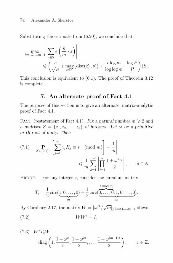
74 Alexander A. Sherstov
Substituting the estimate from (6.20), we conclude that
maxk=1,2,...,m−1
∣∣∣∣∣∑s∈S
e
(k
m· s)∣∣∣∣∣
6
(c√R
+ maxp∈Pdisc(Sp, p)+
c logm
log logm· logP
P
)|S|.
This conclusion is equivalent to (6.1). The proof of Theorem 3.12is complete.
7. An alternate proof of Fact 4.1
The purpose of this section is to give an alternate, matrix-analyticproof of Fact 4.1.
Fact (restatement of Fact 4.1). Fix a natural number m > 2 anda multiset Z = z1, z2, . . . , zn of integers. Let ω be a primitivem-th root of unity. Then
(7.1)
∣∣∣∣∣ PX∈0,1n
[n∑j=1
zjXj ≡ s (mod m)
]− 1
m
∣∣∣∣∣6
1
m
m−1∑k=1
∣∣∣∣∣n∏j=1
1 + ωkzj
2
∣∣∣∣∣ , s ∈ Z.
Proof. For any integer z, consider the circulant matrix
Tz =1
2circ(1, 0, . . . , 0︸ ︷︷ ︸
m
) +1
2circ(
z mod m︷ ︸︸ ︷0, . . . , 0, 1, 0, . . . , 0︸ ︷︷ ︸
m
).
By Corollary 2.17, the matrix W = [ωjk/√m]j,k=0,1,...,m−1 obeys
WW ∗ = I,(7.2)
(7.3) W ∗TzW
= diag
(1,
1 + ωz
2,1 + ω2z
2, . . . ,
1 + ω(m−1)z
2
), z ∈ Z.
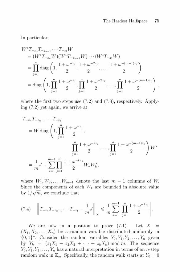
The Hardest Halfspace 75
In particular,
W ∗T−znT−zn−1 · · ·T−z1W= (W ∗T−znW )(W ∗T−zn−1W ) · · · (W ∗T−z1W )
=n∏j=1
diag
(1,
1 + ω−zj
2,1 + ω−2zj
2, . . . ,
1 + ω−(m−1)zj
2
)
= diag
(1,
n∏j=1
1 + ω−zj
2,n∏j=1
1 + ω−2zj
2, . . . ,
n∏j=1
1 + ω−(m−1)zj
2
),
where the first two steps use (7.2) and (7.3), respectively. Apply-ing (7.2) yet again, we arrive at
T−znT−zn−1 · · ·T−z1
= W diag
(1,
n∏j=1
1 + ω−zj
2,
n∏j=1
1 + ω−2zj
2, . . . ,
n∏j=1
1 + ω−(m−1)zj
2
)W ∗
=1
mJ +
m−1∑k=1
n∏j=1
1 + ω−kzj
2WkW
∗k ,
where W1,W2, . . . ,Wm−1 denote the last m − 1 columns of W.Since the components of each Wk are bounded in absolute valueby 1/
√m, we conclude that
(7.4)
∥∥∥∥T−znT−zn−1 · · ·T−z1 −1
mJ
∥∥∥∥∞6
1
m
m−1∑k=1
∣∣∣∣∣n∏j=1
1 + ω−kzj
2
∣∣∣∣∣ .We are now in a position to prove (7.1). Let X =
(X1, X2, . . . , Xn) be a random variable distributed uniformly in0, 1n. Consider the random variables Y0, Y1, Y2, . . . , Yn givenby Yk = (z1X1 + z2X2 + · · · + zkXk) mod m. The sequenceY0, Y1, Y2, . . . , Yn has a natural interpretation in terms of an n-steprandom walk in Zm. Specifically, the random walk starts at Y0 = 0
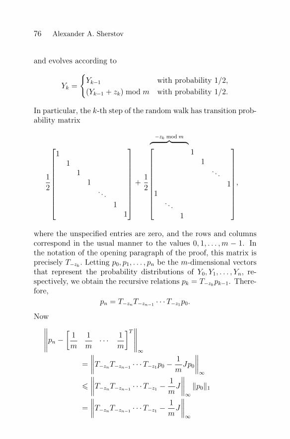
76 Alexander A. Sherstov
and evolves according to
Yk =
Yk−1 with probability 1/2,
(Yk−1 + zk) mod m with probability 1/2.
In particular, the k-th step of the random walk has transition prob-ability matrix
1
2
11
11
. . .
11
+
1
2
−zk mod m︷ ︸︸ ︷
11
. . .
11
. . .
1
,
where the unspecified entries are zero, and the rows and columnscorrespond in the usual manner to the values 0, 1, . . . ,m − 1. Inthe notation of the opening paragraph of the proof, this matrix isprecisely T−zk . Letting p0, p1, . . . , pn be the m-dimensional vectorsthat represent the probability distributions of Y0, Y1, . . . , Yn, re-spectively, we obtain the recursive relations pk = T−zkpk−1. There-fore,
pn = T−znT−zn−1 · · ·T−z1p0.
Now∥∥∥∥∥pn −[
1
m
1
m· · · 1
m
]T∥∥∥∥∥∞
=
∥∥∥∥T−znT−zn−1 · · ·T−z1p0 −1
mJp0
∥∥∥∥∞
6
∥∥∥∥T−znT−zn−1 · · ·T−z1 −1
mJ
∥∥∥∥∞‖p0‖1
=
∥∥∥∥T−znT−zn−1 · · ·T−z1 −1
mJ
∥∥∥∥∞
The Hardest Halfspace 77
61
m
m−1∑k=1
∣∣∣∣∣n∏j=1
1 + ω−kzj
2
∣∣∣∣∣=
1
m
m−1∑k=1
∣∣∣∣∣n∏j=1
1 + ωkzj
2
∣∣∣∣∣ ,where the next-to-last step uses (7.4). This conclusion is obviouslyequivalent to (7.1).
Acknowledgements
This work was supported by NSF CAREER award CCF-1149018and an Alfred P. Sloan Foundation Research Fellowship. I amthankful to Mark Bun, T. S. Jayram, Ryan O’Donnell, RoccoServedio, and Justin Thaler for valuable comments on this work.Special thanks to T. S. Jayram for allowing me to include his shortand elegant proof of Fact 4.1.
References
Scott Aaronson & Yaoyun Shi (2004). Quantum lower bounds forthe collision and the element distinctness problems. J. ACM 51(4),595–605.
Miklos Ajtai, Henryk Iwaniec, Janos Komlos, Janos Pintz& Endre Szemeredi (1990). Construction of a thin set with smallFourier coefficients. Bulletin of the London Mathematical Society 22(6),583–590.
Michael Alekhnovich, Mark Braverman, Vitaly Feldman,Adam R. Klivans & Toniann Pitassi (2008). The complexity ofproperly learning simple concept classes. J. Comput. Syst. Sci. 74(1),16–34.
Noga Alon (1986). Eigenvalues, geometric expanders, sorting inrounds, and Ramsey theory. Combinatorica 6(3), 207–219.
Noga Alon & Yuval Roichman (1994). Random Cayley graphs andexpanders. Random Struct. Algorithms 5(2), 271–285.
78 Alexander A. Sherstov
Noga Alon & Joel Spencer (2008). The Probabilistic Method. JohnWiley & Sons, 3rd edition.
Andris Ambainis (2005). Polynomial degree and lower bounds inquantum complexity: Collision and element distinctness with smallrange. Theory of Computing 1(1), 37–46.
Andris Ambainis, Andrew M. Childs, Ben Reichardt, RobertSpalek & Shengyu Zhang (2010). Any AND-OR formula of size Ncan be evaluated in time N1/2+o(1) on a quantum computer. SIAM J.Comput. 39(6), 2513–2530.
Rosa I. Arriaga & Santosh Vempala (2006). An algorithmic theoryof learning: Robust concepts and random projection. Mach. Learn.63(2), 161–182.
James Aspnes, Richard Beigel, Merrick L. Furst & StevenRudich (1994). The expressive power of voting polynomials. Combi-natorica 14(2), 135–148.
Laszlo Babai, Peter Frankl & Janos Simon (1986). Complex-ity classes in communication complexity theory. In Proceedings of theTwenty-Seventh Annual IEEE Symposium on Foundations of ComputerScience (FOCS), 337–347.
Laszlo Babai, Noam Nisan & Mario Szegedy (1992). Multipartyprotocols, pseudorandom generators for logspace, and time-space trade-offs. J. Comput. Syst. Sci. 45(2), 204–232.
Robert Beals, Harry Buhrman, Richard Cleve, MicheleMosca & Ronald de Wolf (2001). Quantum lower bounds by poly-nomials. J. ACM 48(4), 778–797.
Paul Beame, Matei David, Toniann Pitassi & Philipp Woelfel(2007). Separating deterministic from nondeterministic NOF multi-party communication complexity. In Proceedings of the Thirty-FourthInternational Colloquium on Automata, Languages and Programming(ICALP), 134–145.
Paul Beame & Trinh Huynh (2012). Multiparty communicationcomplexity and threshold circuit size of AC0. SIAM J. Comput. 41(3),484–518.
The Hardest Halfspace 79
Richard Beigel (1994). Perceptrons, PP, and the polynomial hierar-chy. Computational Complexity 4, 339–349.
Richard Beigel, Nick Reingold & Daniel A. Spielman (1995).PP is closed under intersection. J. Comput. Syst. Sci. 50(2), 191–202.
Avrim Blum & Ravindran Kannan (1997). Learning an intersec-tion of a constant number of halfspaces over a uniform distribution. J.Comput. Syst. Sci. 54(2), 371–380.
Avrim Blum & Ronald L. Rivest (1992). Training a 3-node neuralnetwork is NP-complete. Neural Networks 5(1), 117–127.
Harry Buhrman, Ilan Newman, Hein Rohrig & Ronaldde Wolf (2007a). Robust polynomials and quantum algorithms. The-ory Comput. Syst. 40(4), 379–395.
Harry Buhrman, Nikolai K. Vereshchagin & Ronald de Wolf(2007b). On computation and communication with small bias. In Pro-ceedings of the Twenty-Second Annual IEEE Conference on Computa-tional Complexity (CCC), 24–32.
Harry Buhrman & Ronald de Wolf (2001). Communication com-plexity lower bounds by polynomials. In Proceedings of the SixteenthAnnual IEEE Conference on Computational Complexity (CCC), 120–130.
Mark Bun, Robin Kothari & Justin Thaler (2020). The poly-nomial method strikes back: Tight quantum query bounds via dualpolynomials. Theory Comput. 16, 1–71.
Ashok K. Chandra, Merrick L. Furst & Richard J. Lipton(1983). Multi-party protocols. In Proceedings of the Fifteenth AnnualACM Symposium on Theory of Computing (STOC), 94–99.
Karthekeyan Chandrasekaran, Justin Thaler, JonathanUllman & Andrew Wan (2014). Faster private release of marginalson small databases. In Proceedings of the Fifth Conference on Innova-tions in Theoretical Computer Science (ITCS), 387–402.
Arkadev Chattopadhyay & Anil Ada (2008). Multiparty commu-nication complexity of disjointness. In Electronic Colloquium on Com-putational Complexity (ECCC). Report TR08-002.
80 Alexander A. Sherstov
Arkadev Chattopadhyay & Nikhil S. Mande (2018). Separationof unbounded-error models in multi-party communication complexity.Theory of Computing 14(21), 1–23.
Benny Chor & Oded Goldreich (1988). Unbiased bits from sourcesof weak randomness and probabilistic communication complexity. SIAMJ. Comput. 17(2), 230–261.
Joel Friedman, Ram Murty & Jean-Pierre Tillich (2006). Spec-tral estimates for Abelian Cayley graphs. Journal of CombinatorialTheory, Series B 96(1), 111–121.
Zvi Galil, Ravi Kannan & Endre Szemeredi (1989). On nontrivialseparators for k-page graphs and simulations by nondeterministic one-tape Turing machines. J. Comput. Syst. Sci. 38(1), 134–149.
John Gill (1977). Computational complexity of probabilistic Turingmachines. SIAM J. Comput. 6(4), 675–695.
Henry W. Gould (1972). Combinatorial Identities: A StandardizedSet of Tables Listing 500 Binomial Coefficient Summations. Morgan-town Printing and Binding Co.
Johan Hastad (1994). On the size of weights for threshold gates.SIAM J. Discret. Math. 7(3), 484–492.
Hamed Hatami, Kaave Hosseini & Shachar Lovett (2020).Sign rank vs discrepancy. In Proceedings of the Thirty-Fifth AnnualIEEE Conference on Computational Complexity (CCC), volume 169 ofLIPIcs, 18:1–18:14.
Wassily Hoeffding (1963). Probability inequalities for sums ofbounded random variables. Journal of the American Statistical As-sociation 58(301), 13–30.
Stasys Jukna (2001). Extremal Combinatorics with Applications inComputer Science. Springer-Verlag, Berlin.
Jeff Kahn, Nathan Linial & Alex Samorodnitsky (1996).Inclusion-exclusion: Exact and approximate. Combinatorica 16(4),465–477.
The Hardest Halfspace 81
Adam Tauman Kalai, Adam R. Klivans, Yishay Mansour &Rocco A. Servedio (2008). Agnostically learning halfspaces. SIAMJ. Comput. 37(6), 1777–1805.
Nicholas M. Katz (1989). An estimate for character sums. Journalof the American Mathematical Society 2(2), 197–200.
Subhash Khot & Rishi Saket (2011). On the hardness of learningintersections of two halfspaces. J. Comput. Syst. Sci. 77(1), 129–141.
Hartmut Klauck (2007). Lower bounds for quantum communicationcomplexity. SIAM J. Comput. 37(1), 20–46.
Adam R. Klivans (2002). A Complexity-Theoretic Approach to Learn-ing. Ph.D. thesis, MIT.
Adam R. Klivans, Philip M. Long & Alex K. Tang (2009).Baum’s algorithm learns intersections of halfspaces with respect to log-concave distributions. In Proceedings of the Thirteenth InternationalWorkshop on Randomization and Computation (RANDOM), 588–600.
Adam R. Klivans, Ryan O’Donnell & Rocco A. Servedio (2004).Learning intersections and thresholds of halfspaces. J. Comput. Syst.Sci. 68(4), 808–840.
Adam R. Klivans & Rocco A. Servedio (2004). Learning DNF in
time 2O(n1/3). J. Comput. Syst. Sci. 68(2), 303–318.
Adam R. Klivans & Rocco A. Servedio (2008). Learning intersec-tions of halfspaces with a margin. J. Comput. Syst. Sci. 74(1), 35–48.
Adam R. Klivans & Alexander A. Sherstov (2009). Crypto-graphic hardness for learning intersections of halfspaces. J. Comput.Syst. Sci. 75(1), 2–12.
Matthias Krause & Pavel Pudlak (1997). On the computationalpower of depth-2 circuits with threshold and modulo gates. Theor.Comput. Sci. 174(1–2), 137–156.
Matthias Krause & Pavel Pudlak (1998). Computing Booleanfunctions by polynomials and threshold circuits. Comput. Complex.7(4), 346–370.
82 Alexander A. Sherstov
Eyal Kushilevitz & Noam Nisan (1997). Communication Complex-ity. Cambridge University Press.
Stephen Kwek & Leonard Pitt (1998). PAC learning intersectionsof halfspaces with membership queries. Algorithmica 22(1/2), 53–75.
Troy Lee & Adi Shraibman (2009). Disjointness is hard in themultiparty number-on-the-forehead model. Computational Complexity18(2), 309–336.
Ka Hin Leung, Vinh Nguyen & Wasin So (2011). Nonexistence ofa circulant expander family. Bulletin of the Australian MathematicalSociety 83(1), 87–95.
Nathan Linial & Noam Nisan (1990). Approximate inclusion-exclusion. Combinatorica 10(4), 349–365.
Nathan Linial & Adi Shraibman (2009). Learning complexity vscommunication complexity. Combinatorics, Probability & Computing18(1-2), 227–245.
Nati Linial, Shahar Mendelson, Gideon Schechtman & AdiShraibman (2007). Complexity measures of sign matrices. Combina-torica 27(4), 439–463.
Marvin L. Minsky & Seymour A. Papert (1969). Perceptrons:An Introduction to Computational Geometry. MIT Press, Cambridge,Mass.
Saburo Muroga (1971). Threshold Logic and Its Applications. JohnWiley & Sons, New York.
J. Myhill & W. H. Kautz (1961). On the size of weights required forlinear-input switching functions. IRE Trans. on Electronic Computers10(2), 288–290.
D. J. Newman (1964). Rational approximation to |x|. Michigan Math.J. 11(1), 11–14.
Ryan O’Donnell & Rocco A. Servedio (2010). New degree boundsfor polynomial threshold functions. Combinatorica 30(3), 327–358.
The Hardest Halfspace 83
Ramamohan Paturi (1992). On the degree of polynomials that ap-proximate symmetric Boolean functions. In Proceedings of the Twenty-Fourth Annual ACM Symposium on Theory of Computing (STOC),468–474.
Ramamohan Paturi & Janos Simon (1986). Probabilistic commu-nication complexity. J. Comput. Syst. Sci. 33(1), 106–123.
A. Razborov, E. Szemeredi & A. Wigderson (1993). Constructingsmall sets that are uniform in arithmetic progressions. Combinatorics,Probability and Computing 2(4), 513–518.
Alexander A. Razborov (2002). Quantum communication com-plexity of symmetric predicates. Izvestiya of the Russian Academy ofSciences, Mathematics 67, 145–159.
Alexander A. Razborov & Alexander A. Sherstov (2010). Thesign-rank of AC0. SIAM J. Comput. 39(5), 1833–1855.
Theodore J. Rivlin (1981). An Introduction to the Approximationof Functions. Dover Publications, New York.
Barkley Rosser (1941). Explicit bounds for some functions of primenumbers. American Journal of Mathematics 63(1), 211–232.
Imre Z. Ruzsa (1987). Essential components. Proceedings of the Lon-don Mathematical Society 53-54(1), 38–56.
Alexander A. Sherstov (2008a). Communication lower bounds us-ing dual polynomials. Bulletin of the EATCS 95, 59–93.
Alexander A. Sherstov (2008b). Halfspace matrices. Computa-tional Complexity 17(2), 149–178.
Alexander A. Sherstov (2009a). Approximate inclusion-exclusionfor arbitrary symmetric functions. Computational Complexity 18(2),219–247.
Alexander A. Sherstov (2009b). Separating AC0 from depth-2 ma-jority circuits. SIAM J. Comput. 38(6), 2113–2129.
Alexander A. Sherstov (2010). Communication complexity un-der product and nonproduct distributions. Computational Complexity19(1), 135–150.
84 Alexander A. Sherstov
Alexander A. Sherstov (2011). The pattern matrix method. SIAMJ. Comput. 40(6), 1969–2000.
Alexander A. Sherstov (2013a). The intersection of two halfspaceshas high threshold degree. SIAM J. Comput. 42(6), 2329–2374.
Alexander A. Sherstov (2013b). Optimal bounds for sign-representing the intersection of two halfspaces by polynomials. Combi-natorica 33(1), 73–96.
Alexander A. Sherstov (2014). Communication lower bounds usingdirectional derivatives. J. ACM 61(6), 1–71.
Alexander A. Sherstov (2016). The multiparty communicationcomplexity of set disjointness. SIAM J. Comput. 45(4), 1450–1489.
Alexander A. Sherstov (2018). On multiparty communication withlarge versus unbounded error. Theory of Computing 14(22), 1–17.
Kai-Yeung Siu & Jehoshua Bruck (1991). On the power of thresh-old circuits with small weights. SIAM J. Discrete Math. 4(3), 423–435.
Jun Tarui & Tatsuie Tsukiji (1999). Learning DNF by approxi-mating inclusion-exclusion formulae. In Proceedings of the FourteenthAnnual IEEE Conference on Computational Complexity (CCC), 215–221.
Justin Thaler (2016). Lower bounds for the approximate degreeof block-composed functions. In Proceedings of the Forty-Third In-ternational Colloquium on Automata, Languages and Programming(ICALP), 17:1–17:15.
Justin Thaler, Jonathan Ullman & Salil P. Vadhan (2012).Faster algorithms for privately releasing marginals. In Proceedings of theThirty-Ninth International Colloquium on Automata, Languages andProgramming (ICALP), 810–821.
Jayram S. Thathachar (1998). On separating the read-k-timesbranching program hierarchy. ECCC Report TR98-002. URL https://
eccc.weizmann.ac.il/report/1998/002. Extended abstract in Pro-ceedings of the Thirtieth Annual ACM Symposium on Theory of Com-puting (STOC), 1998.
The Hardest Halfspace 85
Leslie G. Valiant (1984). A theory of the learnable. Commun. ACM27(11), 1134–1142.
Santosh Vempala (2010). A random-sampling-based algorithm forlearning intersections of halfspaces. J. ACM 57(6), 32.
Andrew Chi-Chih Yao (1979). Some complexity questions relatedto distributive computing. In Proceedings of the Eleventh Annual ACMSymposium on Theory of Computing (STOC), 209–213.
E. I. Zolotarev (1877). Application of elliptic functions to questionsof functions deviating least and most from zero. Izvestiya Imp. Akad.Nauk 30(5).
Manuscript received 31 July 2019
Alexander A. SherstovComputer Science DepartmentUCLALos Angeles, CA 90095 [email protected]