- 1 -

THE HIGH CURRENT TRANSPORT EXPERIMENT FOR HEAVY

ION INERTIAL FUSION1

L. R. Prost, D. Baca, F. M. Bieniosek, C.M. Celata, A. Faltens, E. Henestroza,

J. W. Kwan, M. Leitner, P.A. Seidl , W. L. Waldron

Lawrence Berkeley National Laboratory, Berkeley, CA 94720 USA

R. Cohen, A. Friedman, D. Grote, S.M. Lund, A.W. Molvik

Lawrence Livermore National Laboratory, Livermore, CA 94550 USA

E. Morse

University of California, Berkeley, CA 94720 USA

Abstract

The High Current Experiment (HCX) at Lawrence Berkeley National Laboratory is part of the US program

to explore heavy-ion beam transport at a scale representative of the low-energy end of an induction linac

driver for fusion energy production. The primary mission of this experiment is to investigate aperture fill

factors acceptable for the transport of space-charge-dominated heavy-ion beams at high intensity (line

charge density ~ 0.2 µC/m) over long pulse durations (4 µs) in alternating gradient focusing lattices of

electrostatic or magnetic quadrupoles. This experiment is testing transport issues resulting from nonlinear

space-charge effects and collective modes, beam centroid alignment and steering, envelope matching,

image charges and focusing field nonlinearities, halo and, electron and gas cloud effects. We present the

results for a coasting 1 MeV K+ ion beam transported through ten electrostatic quadrupoles. The

measurements cover two different fill factor studies (60% and 80% of the clear aperture radius) for which

the transverse phase-space of the beam was characterized in detail, along with beam energy measurements

1 This work performed under the auspices of the U.S Department of Energy by University of California, Lawrence Livermore and Lawrence Berkeley National Laboratories under contracts No. W-7405-Eng-48 and DE-AC03-76SF00098

- 2 -

and the first halo measurements. Electrostatic quadrupole transport at high beam fill factor (80%) is

achieved with acceptable emittance growth and beam loss, even though the initial beam distribution is not

ideal (but the emittance is low) nor in thermal equilibrium. We achieved good envelope control, and re-

matching may only be needed every ten lattice periods (at 80% fill factor) in a longer lattice of similar

design. We also show that understanding and controlling the time dependence of the envelope parameters is

critical to achieving high fill factors, notably because of the injector and matching section dynamics.

- 3 -

1. INTRODUCTION

The High Current Experiment (HCX) [1], located at Lawrence Berkeley National Lab and carried

out by the HIF-VNL2, is designed to explore the physics of intense beams in the context of developing a

heavy-ion high-intensity accelerator (i.e. driver) for an inertial fusion power plant [27,28].

At an injection energy of 1-1.8 MeV, a line-charge density, λ, of 0.1-0.2 µC m-1 and a pulse

duration of 4 µs, the HCX main beam parameters are in the range of interest for a fusion driver front-end.

At 1 MeV where we performed our experiments, the generalized beam perveance is

43

0

108)(4

2 −×==cm

qIK B

βγπε. (1)

In this regime space-charge forces strongly influence the beam properties during its transport, and image

charges induced on metallic structures of the machine aperture play an important role. For comparison, the

beam line-charge density and generalized perveance of large accelerator facilities such as the Spallation

Neutron Source (SNS) Front End [29,30,31] and Fermilab’s Linac Experimental Facility [32,33,34] are one

to two orders of magnitude lower than the HCX parameters. Also, in both cases, the beam is rapidly

accelerated to energies where space-charge effects are diminished. For heavy-ion inertial fusion, where the

line-charge density increases from 0.2 µC m-1 at injection to 1.7 µC m-1 at the end of the accelerator

(4.0 GeV, Bi+) and approximately 30 µC m-1 at the end of the drift compression at the D-T target [42], the

perveance is increased by beam bunch compression as part of the acceleration schedule, which optimizes

the induction linear accelerator efficiency.

Previous scaled experiments at LBNL [43,44,46,47] were designed with the appropriate perveance

for studying driver-like phenomena, principally transport with sufficient current to highly depress the single

particle betatron tunes, but the beam current was kept relatively low. For example, in the Single Beam

Transport Experiment (SBTE) [35], the maximum generalized perveance was 2.2 x 10-3 - higher than

generally envisioned for a fusion driver - but the line charge density remained about one order of

magnitude lower than for the HCX or a fusion driver front end. The University of Maryland Electron Ring

2 Heavy-Ion Fusion Virtual National Laboratory: a collaboration between groups at LBNL, LLNL and Princeton Plasma Physics Laboratory, pursuing the common beam science for high energy density physics and inertial fusion energy.

- 4 -

(UMER) [36], which was designed for studying the transport of high intensity electron beams in a strong

focusing lattice, can also produce highly tune-depressed beams with a line charge density of

λ 1.5 × 10-3 µC m-1 [37].

A principal goal of the HCX experiment is to evaluate the maximum acceptable beam fill factor,

i.e. the maximum radial extent of the beam within the physical aperture (i.e. borebeam rr / , where beamr is

the maximum envelope excursion (2× RMS) of a beam propagating in a transport channel of radius borer ,

which is the physical clear bore radius inside the quadrupoles), addressing the question of how compact a

multiple-beam focusing lattice can be to accommodate the transport and acceleration of the heavy-ion

beams. Higher fill factors are desirable because they make more economically efficient use of material

structures. For example, cost savings of 50% have been projected in multi-beam drivers if the fill factor can

be increased from 60% to 80% [63]. The fill factor study in this experiment addresses the more

fundamental issue of how much charge can be transported in a single channel without beam loss or

deterioration of the beam quality. Greater fill factors enhance non-ideal physics effects resulting from

imperfect focusing optics, images charge and halo impacting material structures and releasing desorbed

gases that interact with long-pulse beams, creating possible electron-cloud effects. These are intense beam

physics issues that may be relevant to other accelerator applications requiring high intensity, such as

spallation neutron sources and the production of rare isotopes. Design and engineering issues such as the

frequency at which the beam coherent oscillation (i.e. centroid) must be corrected for, or the alignment

tolerances for the focusing elements, are also less favorable the greater the fill factor and are also addressed.

The HCX beam transport line is at present mainly based on an alternating gradient (AG)

electrostatic quadrupole focusing (i.e. quadrupoles with equal voltages alternating in sign), which provides

efficient transport at low energy. Secondary electrons are expected to be swept out of the beam path by the

quadrupole fields and are not anticipated to set transport limits. In follow-up experiments, transport-

limiting effects in magnetic quadrupoles due to electrons are being explored. In that situation, electrons can

be trapped by the beam self-potential and disrupt the beam dynamics.

The organization of this paper is as follows: in Sec. 2 we present the apparatus including the

diagnostics, in Sec. 3 and 4 we show beam measurements from the injector and the matching section, in

Sec. 5 we discuss the beam current time dependence and the consequences on the beam envelope and beam

- 5 -

control, in Sec. 6 we show the fill factor results for the transport through electrostatic quadrupoles, in Sec. 7

we discuss the features of the measured beam charge distribution., in Sec. 8 we present the beam energy

measurements, in Sec. 9 we discuss the main results of our experiments. Conclusions and implications for

future heavy-ion accelerators are in Sec. 10.

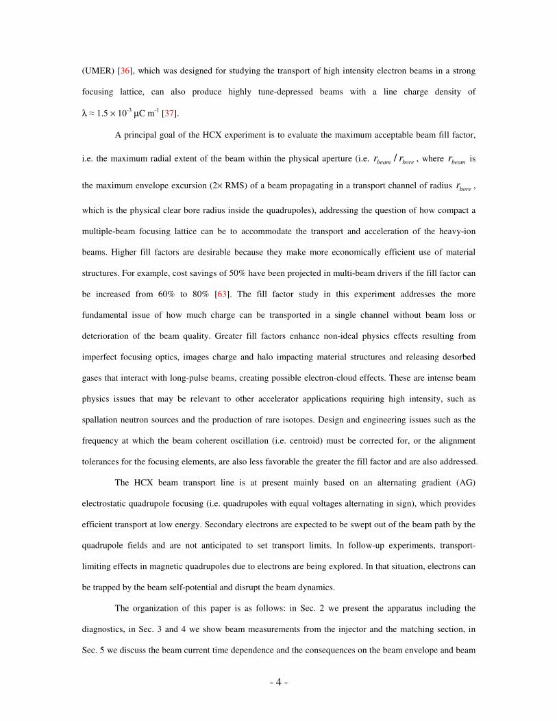
2. EXPERIMENTAL CONFIGURATION

The present configuration consists of the K+ ion source and injector, an electrostatic quadrupole

matching section (six quadrupoles), ten electrostatic transport quadrupoles and four room-temperature

pulsed magnetic quadrupoles. A multi-purpose diagnostic station (D-end) is at the end of the beam line

(Fig. 1). This paper discusses the results from the electrostatic transport section.

Figure 1: (Color) Layout of the HCX (elevation view).

A. Injector

The injector consists of a 10.0-cm-diameter hot surface ionization source assembly followed by a

750 kV extraction diode, then by four electrostatic quadrupoles (ESQ) biased to focus the beam

transversely while accelerating longitudinally (up to 2 MV) [57,58]. Figure 2 shows the source assembly,

the gate electrode that provides the extraction and the ESQ column.

11 m

D-end, Energy Analyzer, GESD

4 RT pulsed magnetic

quadrupoles

TOF pulser

1-1.8 MeV ESQ Injector

Matching section (6 quadrupoles)

10 electrostatic transport quadrupoles

Current monitor QD1 D2

K+ source & diode

I = 0.2-0.6 A

- 6 -

Figure 2: (Color) 2 MV injector accelerator column showing fiberglass support struts. The column length

is 2.4 meters. The red part in the insert shows the addition to the gate electrode reducing its aperture

diameter from 179.5 mm to 110 mm.

The injector is contained inside a pressure vessel, filled with a high-voltage insulating gas mixture

(90% N2 and 10% SF6). The vessel houses 38 stages of a two-section network Marx generator, which

produces a flat-top voltage pulse (VMarx), and a high voltage ‘dome’ containing the source and extraction

pulse electronics. The high voltage dome also houses a hydraulically-driven 400 Hz, 10 kVA alternator

Ion source assembly

Diode section

Support collar

ESQ section

Fiberglass support strut

ESQ electrode

Electrode plate HV Dome

Source emitter

Pierce electrode

Gate electrode

Electron trap

- 7 -

which powers all the source electronics, including the telemetry system. Voltages to the various electrodes

of the diode and accelerating column are obtained from a sodium sulfate solution water resistor (i.e. water

resistor, R 5 kΩ). The source is biased at a negative DC potential (VBias) while the gate electrode is tied to

the potential of the dome, inhibiting ion emission from the hot surface. During ion extraction, the extraction

circuit, which controls most of the emission, delivers a pulse swing (VGate) up to 140 kV, going from a bias

voltage of -60 kV to an extraction voltage of +80 kV, applied to the source with respect to the gate

electrode through a step-up transformer driven by a tunable pulse forming network (PFN) [2,5]. Note that

the source filament transformer not only supplies the heater power (2.5 kW), but is also a high voltage

isolation transformer allowing the source to be biased at up to -80 kV. Trigger, timing, and diagnostics

information are transmitted to and from the high voltage dome by analog fiber optics links.

Figure 3 shows the Marx pulse and the gate pulse with their respective timings.

Figure 3: (Color) Typical Marx (blue) and gate (red) pulses. The Marx pulse is viewed through a

capacitive monitor, whose gain is 21.4 kV/V. The gate pulse is viewed through a resistive divider and an

optical link. In green, we show the negative DC bias that is applied to the source. Note that the ripples seen

-5

0

5

10

15

20

25

30

35

40

45

-1.0 1.0 3.0 5.0 7.0 9.0 11.0 13.0 15.0

Time [µµµµsec]

Mar

x vo

ltage

mon

itor

[V]

-0.5

0.0

0.5

1.0

1.5

2.0

Gat

e vo

ltage

mon

itor

[V]

Marx pulseGate pulse

Extraction voltage

Negative Bias offset

- 8 -

on the gate voltage early and during the flattop of the pulse are due to electrical noise picked up on the

cables when the trigger chassis of the Marx column fires.

The gate pulse length is 4.5 µs flattop. Over that time, the Marx pulse is flat to within 1.4%. The repetition

rate is 0.1 Hz at 1 MeV.

The Marx voltage drifts due to changes in the conductivity of the water resistor. We keep the peak

beam energy ( BE ) within ±0.5% of its nominal value by monitoring the Marx voltage pulse output with a

capacitive probe and adjusting the Marx charging power supplies set point accordingly. Moreover, the

beam current ( BI ) also drifts by several percent if left uncorrected during an ~8 hour period. This drift is

attributed to electronics and possibly material effects in the source. Therefore, beam parameters are also

kept constant by empirically adjusting the charge voltage of the gate electrode pulser to maintain a constant

averaged beam current.

At beam energies higher than ~ 1.5 MeV, operation is complicated by the fact that the water

resistor partially deforms under the higher required dome pressure load, affecting the voltage division along

the accelerating column and modifying the injector optics [5].

B. Matching section

The matching section (Fig. 4) consists of six electrostatic quadrupoles (QM1-QM6) designed to

compress the beam area transversely by a factor 25 and produce the matched beam parameters for

transport in the periodic electrostatic lattice.

- 9 -

Figure 4: Mechanical drawing (elevation view) of the matching section. On the left is the injector. On the

right is the first quadrupole of the transport section (QD1) which is movable to allow room for diagnostics.

The radii of the first (QM1) and last (QM6) matching quadrupole bores are borer = 100 mm and

31 mm respectively. Each quadrupole is independently energized and the power supplies are remotely

controlled and monitored via Ethernet links. Matching quadrupole voltages range up to ±43 kV for

EB = 1.0 MeV, and focusing gradients up to 9 kV/cm2 are produced by the lattice (Quadrupole potentials

scale linearly with the beam energy).

Residual misalignment of the source in the diode region, non-uniformities in the source’s current

density distribution and alignment of the focusing elements of the injector and matching section drive

betatron oscillations of the beam centroid through the quadrupoles of the matching section. QM4-6 may

each be moved in the horizontal and vertical directions by up to ±15 mm to correct the beam centroid offset.

QM2 QM3

QM4

QM1

QM5

QM6

QD1

311.4 cm

∅18.0 cm ∅17.0 cm ∅13.4 cm ∅9.8 cm

- 10 -

C. Electrostatic transport section

The transport section consists of 10 electrostatic quadrupoles on a common supporting rail (Fig. 5).

The quadrupoles are aligned to within ±100 µm on the bench before installation inside the vacuum tank.

Figure 5: Cutaway view of the electrostatic transport section.

The rail is mounted on a six-strut/kinematic system, with alignment fiducials outside the vacuum

chamber, decoupling it from the vacuum tank. It is then aligned independently to the rest of the beam line.

The first quadrupole (QD1) is movable, allowing insertion in its place of various diagnostics to measure the

beam properties before transport. The last two quadrupoles (QI9 and QI10) may be displaced (horizontal

and vertical directions) to correct betatron centroid oscillations. Additionally, QD1 can be rotated by two or

four degrees for studying the effect of rotated quadrupoles on the beam. QD1 and QI7 to QI10 are

independently biased. The second to sixth quadrupoles (Q2 to Q6) are energized in parallel. For QI7 to

QI10, each feedthrough supplies independent voltages to adjacent quadrupoles, preventing a voltage

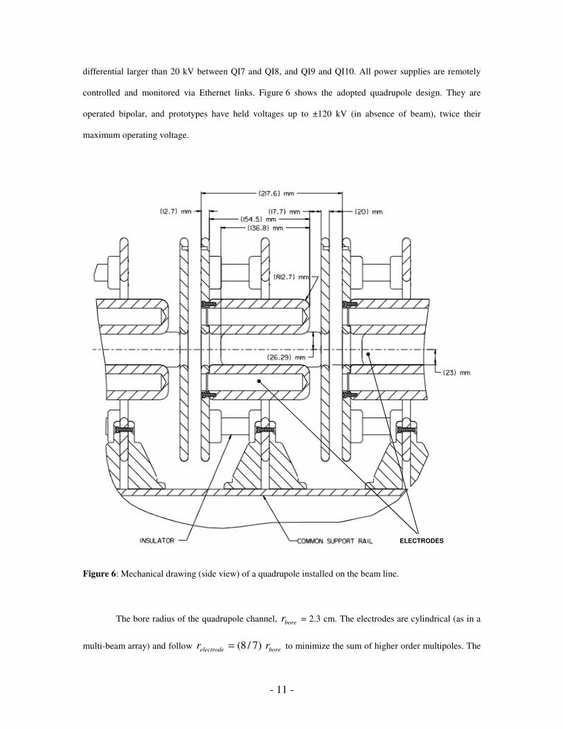
- 11 -

differential larger than 20 kV between QI7 and QI8, and QI9 and QI10. All power supplies are remotely

controlled and monitored via Ethernet links. Figure 6 shows the adopted quadrupole design. They are

operated bipolar, and prototypes have held voltages up to ±120 kV (in absence of beam), twice their

maximum operating voltage.

Figure 6: Mechanical drawing (side view) of a quadrupole installed on the beam line.

The bore radius of the quadrupole channel, borer = 2.3 cm. The electrodes are cylindrical (as in a

multi-beam array) and follow boreelectrode rr )7/8(= to minimize the sum of higher order multipoles. The

ELECTRODES

- 12 -

drift length between two quadrupole end-plates is 2 cm and the half-lattice period, L = 217.6 mm. A

calculation of the electrostatic field based on the mechanical design showed very good field quality with

integrated higher order multipoles equal to 0.73% of the integrated quadrupole component at a radius

r = 2 cm from the center of the quadrupole, down to 0.24% at r = 1.5 cm and 0.06% at r = 1 cm. The

effective length of the quadrupole moment )(zEQr , defined as ( ) )0()( == zEdzzEl QrQreff ,

where z = 0 is the center of the quadrupole, is 151.5 mm. The lattice longitudinal occupancy (i.e. Lleff / )

is η = 0.70.

D. Diagnostics

Beam diagnostics are located at the interface of the matching section and the ten transport

quadrupoles section (QD1), after the last transport quadrupole in the periodic lattice (D2) and at the end of

the beam line (D-end) (see Fig. 1). At the early stages of the experiment, the apparatus did not include the

D2 diagnostics station and the magnetic quadrupoles. Instead, the electrostatic lattice was directly coupled

to the D-end diagnostics tank. The z locations of the D2 phase-space measuring planes since March 2003

are 5.5 cm (horizontal) and 8.6 cm (vertical) upstream of the D-end measuring planes prior to March 2003.

Note that all data taken at the exit of the electrostatic transport section (‘D-end data’ before March 2003,

‘D2 data’ after March 2003) will be referred to as ‘D2 data’, unless otherwise specified.

When making measurements at QD1, the first quadrupole of the electrostatic transport section is

moved out of the beam path via a vacuum feedthrough and lead screw assembly, and the selected

diagnostics are moved in. There is no quadrupole at D2, so that after QI10 there is a drift of 15.2 cm to the

first magnetic quadrupole. All diagnostics stations include transverse slit scanners and Faraday cups (with

an additional current transformer at QD1). A large current transformer at the exit of the injector monitors

the total beam current. The total current measurements are accurate to ±1%.

Transverse slit scanners consist of pairs of paddles (moving horizontally and/or vertically) holding

stainless steel slits and slit-cups (i.e. a compact assembly composed of a shallow Faraday cup or simple

collector plate located behind a masking slit). Each paddle is independently driven by a computer-

controlled step motor, with a positioning accuracy of 10 µm. The step motors reside outside the vacuum

- 13 -

system and drive the diagnostic slit (or slit-cup) via a ferrofluidic seal and lead screw assembly. Depending

on the diagnostic station, slits are 25 or 50 µm wide and 7 to 20 cm long. Slit-cups are biased such that

secondary electrons amplify the collected incident ion signal by a factor of 40.

Stepping through the beam with a slit-cup gives a transverse current density profile. This

measurement integrates over the current density in the plane perpendicular to the motion of the slit-cup. For

instance, for a horizontal profile ( x -direction), where the slit is oriented vertically ( y -direction), the

measured signal is proportional to

= dytyxJtx ),,(),(ρ ,

and similarly in the other (y) direction, where ),,( tyxJ is the beam current density as a function of time.

These measurements determine the beam centroid and radius in one of the transverse planes. They also

indicate large-scale asymmetries or distortions of the distribution from “ideal” uniform density elliptical

cross-sections. The signal-to-noise ratio for profile measurements ranges from 15:1 to 500:1 depending on

the slit width and the current density at the location of the measurement.

The projected phase-space distribution of the beam [ ),,( txxf ′ or ),,( tyyf ′ ] is measured with

a slit and a parallel slit-cup. The slit is located 10 - 15 cm upstream of the slit-cup and determines the

position coordinate, x or y of the beam being sampled. The slit-cup is then scanned through the

transmitted slice to measure the transverse velocity distribution ( x′ or y′ ) at that position. The drift

distance between the slit and the slit-cup is chosen such that < 1% of the measured transverse envelope

expansion of the transmitted slice is due to the remaining space-charge forces. This procedure is repeated to

map phase-space density projections [35,19,59]. The signal-to-noise ratio varies from 10:1 to 300:1

depending on the diagnostic station and the current density at the collector.

A slit and slit-cup pair oriented perpendicular to each other is used to map out the current density

distribution in the plane perpendicular to the beam motion, ),,( tyxJ [19]. The upstream slit determines

one position coordinate, x or y and the slit-cup the other, y or x . The difference between this and the

phase-space measurements described above is that the downstream slit is scanning through the long

dimension of the transmitted sheet beam. This is illustrated in Fig. 7.

- 14 -

Figure 7: (Color) Schematic illustrating the current density mapping procedure.

This results in a smaller signal amplitude, but the high intensity beam allows this procedure to be

carried out with good signal-to-noise ratio (15:1). A Kapton film was also used to produce time-integrated

images of the beam [4]. Kapton is an organic polymer that degrades when exposed to the beam. This

degradation results in a darkening of the film which indicates the time-integrated beam current distribution.

Kapton has linear dose response over the range of interest and excellent spatial resolution. It also

discriminates against low energy and low mass particles (e.g.: electrons).

All these measurements (except for the Kapton image) are time-resolved with a typical resolution

of 40 to 120 ns. The minimum time resolution is of the order of 10 ns, limited by the transit time of the ions

through the slit-cup detector and the capacitance of the circuit (including the collector). They rely on the

beam properties being both reproducible from shot to shot and also over long periods of times. Forty to 275

pulses are required for transverse profile and phase-space measurements, and 3500-4000 for the full current

density distribution. The stability of the injector is adequate and will be addressed in a later section. The

power supplies that energize the quadrupoles of the matching and transport sections are stable to ±0.1%.

Shot-to-shot variations in BI and BE contribute to overall uncertainties, which are folded into the

evaluation of the uncertainties of the envelope parameters and emittance.

All data collected with the mechanical slit scanners are analyzed with routines written in Matlab™

[55]. These routines allow quick manipulation of the data such as background subtraction and extraction of

the first and second moments of the beam distribution used in the calculation of the emittance. Various

plots are also generated, including phase-space diagrams as a function of time. Signals with less than 2-6%

Beam

Upstream slit Downstream slit

x

y

x

y

Current density map

- 15 -

of the peak amplitude are rejected for the calculation of the moments, depending on the diagnostics station.

The statistical beam envelope radii and angles ( a , a′ , b and b′ ) are defined in Appendix A.

The last two of four quadrupole magnets are being instrumented with diagnostics specifically

designed to explore beam-gas and electron-cloud issues (e.g.: flush probes, gridded probes, ion and electron

energy analyzers) [7].

A Gas and Electron Source Diagnostic (GESD) [7] is located at the end of the diagnostics tank (D-

end) and is used to measure electron emission and gas desorption yields from ions incident on targets near

grazing incidence ion angle. These data are intended for calibration of the signal intensities collected on the

flush-probe electrodes in the magnetic quadrupoles so that the beam loss and the gas desorption rate may be

inferred. The GESD can also be used to study mitigation techniques for such undesirable effects.

The GESD can be removed and replaced with an Electrostatic Energy Analyzer (EA). The EA is

used for direct beam kinetic energy measurements but also provides time-dependent longitudinal phase-

space information. The EA, a 90°-spectrometer with a radius of 46 cm, and a gap between the two

electrodes of 2.5 cm, was operated up to ∆V = 110 kV, corresponding to a beam energy of 0.9 MeV. The

relative accuracy is ±0.2%, allowing detection of small energy variations as a function of time during the

beam pulse. The absolute calibration depends on the geometry and fringe fields of the analyzer. By

changing the beam energy by a known absolute amount, we were able to provide an independent

calibration: The beam passed through a 28%-transparent hole-plate, and the gas cloud created at the biased

hole-plate stripped some singly charged K+ beam ions to doubly charged K2+, which were detected in the

analyzer. Thus, the absolute beam mean energy is measured to ±2%.

Beam energy measurements can also routinely be done by a time-of-flight (TOF) technique. A fast

pulser in the matching section (0.3 µs FWHM) induced 1% energy perturbations near the middle of the

beam pulse. These energy pulses manifest as 5-10% current perturbations when measured 5.4 m

downstream. They have been used as a time stamp for an accurate determination of the time of flight of the

particles. The TOF measurements are accurate to ±2%. This is more accurate than, for example, measuring

the TOF by detection of the arrival time of a current equal to 50% of maximum of the beam rise time

because the longitudinal space charge of the beam at the head (and tail) modify the longitudinal distribution

and measured arrival times

- 16 -

Additionally, a prototype optical diagnostic [21] is installed in the D-end tank and a more compact

optical diagnostic subsequently developed is installed at D2. They consist of movable slits ( x - or y -

direction) that intercept the beam, and a thin sheet of scintillator material placed in the path of the

transmitted sheet beam. The light resulting from the ions interacting with the scintillator material is then

captured through an optical window with a gated CCD camera located outside the vacuum chamber [21].

The function of the optical diagnostic is equivalent to the slit scanner described above with the additional

advantage of providing additional information about the 4-D beam distribution [i.e. ),,( tyxf ′ and

),,( txyf ′ ] rather than integrated slit projection, because intensity along the slit is also measured. Used

with an ensemble of pinholes, it would measure the full transverse 4-D distribution. They also allow for a

much faster data acquisition time for equivalent spatial and angular resolution. The light intensity

distribution is later analyzed to derive the second moments and emittance of the beam. These images are

also compiled to give a ),( yxJ distribution of the beam. Though it is possible to image the whole beam

directly onto the scintillator to get its transverse current density distribution in a single pulse, the light

output of the scintillator material degrades under high-intensity bombardment.

Finally, all of the electrostatic quadrupoles are biased through coupling circuits, allowing them to

act as capacitive pickups and beam loss monitors when the beam passes. When in a quadrupole, the beam

induces image charges onto the electrodes. As the charge subtended by the quadrupole electrodes builds up

(or decreases), a current flows through the coupling circuit and a voltage drop appears across the resistor

MonitorR such that we can measure:

dttdQ

RtV Monitor

)()( 0= , (2)

where )(0 tQ is the total charge within the quadrupole at time t and is proportional to the beam current,

BI . For a trapezoidal current pulse (square pulse with linear rise and fall times), the resulting capacitive

pickup signal is a positive and negative peak separated by the beam duration. Secondary particles (ions and

electrons) resulting from direct interaction with the electrodes will travel from one electrode to another (of

the opposite polarity). Since electrodes are biased in pairs and monitored through the same coupling circuit,

this displacement of charges induces a current that will be measured in addition to the capacitive effect. In

- 17 -

particular, the collection of lost ions and emission of secondary electrons during the ‘flattop’ of the beam

pulse generates a signal (negative for positively biased electrode pairs and positive for negatively biased

electrode pairs) proportional to the beam losses. The pickup signal due to lost ions is amplified by the large

secondary electron coefficient (a parametric fit from data taken from 80° to 88° gives θγ 1cos7 −≅e ,

where θ = 0° indicates normal incidence to the surface [7]; typical angles of lost ions are expected to be

near grazing where eγ is maximal), making this diagnostic more sensitive to beam loss than comparisons

of the total beam current data at different locations along the beam line. They additionally indicate regions

of the lattice where envelope excursions and centroid offsets cause particle loss from scraping. However,

since the collected signal is directly proportional to eγ , which depends on the angle of incidence of the

ions on the electrodes, the uncertainty on the absolute value of the current loss is large. For interpretation of

the pickup signals, an effective secondary electron yield 50 < eγ~ < 100 is assumed. Viewed through

MonitorR = 10 Ω, a pickup signal amplitude of 1 V corresponds to 1 mA < lossBI < 2 mA.

At a pressure of 10-7 Torr, beam loss due to beam-background gas interactions over the length of

the electrostatic transport section (2.2 m) is expected to be approximately 0.025% (e.g.: lossBI = 0.04 mA

for BI = 175 mA), dominated by stripping (K+ K2+, ++ → 2KKσ = 3.5 × 10-16 cm2 [6]), assuming that the

background gas mostly consists of N2 and/or O2.

E. Numerical simulations

Envelope codes are useful during the design process to determine the main lattice parameters and

for controlling and tuning the beam during operation. The coupled envelope equations

0)(

23

2

=−+

−+′′aba

Kaka xε

, (3a)

0)(

23

2

=−+

−−′′bba

Kbkb yε

, (3b)

are numerically integrated, where

- 18 -

RMSyxyx ,, 4εε = (4)

is the unnormalized ‘edge emittance’ of the beam in the horizontal and vertical directions, respectively, and

RMSyx,ε are defined in Appendix A (Eq. A2). In Eqs. (3a) and (3b), K is the generalized perveance

defined in Eq. (1) and k is the strength of the applied focusing fields. The main difference between the

various envelope codes is how the applied fields are described. The simplest description of these fields is

the hard-edge equivalent model of the quadrupoles. The focusing fields are then given by

2

1

boreB

q

rE

Vk = ,

where qV is the quadrupole unipolar voltage, and is applied over the effective length of the quadrupole. A

more realistic model employs the quadrupole component of the multipole decomposition of the 3-D field

based on the quadrupole geometry, and the effect of the Ez component of the applied fields on the envelope

and corresponding radial focusing force arising from the varying kinetic energy.

However, the envelope model only describes the statistical edge evolution of the beam and does

not include higher order components of the focusing fields or the effect of the image forces that become

more important when the beam gets close to the walls. Moreover, other effects like the behavior of halo

particles (i.e. particles whose trajectories reside outside the core of the beam) or collective effects such as

space-charge waves and nonlinear self fields are not addressed in an envelope description of the beam and

may alter its dynamics. In order to consider the high-intensity beams needed for heavy-ion inertial fusion,

we need to take all these effects into consideration. The dynamics of the beam can be studied by calculating

the trajectories of many macroparticles, each representing a large number of actual beam particles. Particle-

in-cell (PIC) codes such as WARP [56,20], quickly described below, follow this principle.

The WARP code uses plasma simulation techniques to model self-consistently the behavior of

high-space-charge particle beams. It allows flexible and detailed multi-dimensional modeling of high

current beams in a wide range of systems, and is being designed and optimized for heavy ion fusion

accelerator physics studies. The core model is the particle-in-cell (PIC) algorithm, which is combined with

a description of the accelerator lattice. At present it incorporates a 3-D field description, an axisymmetric

( zr, ) description, a transverse slice ( yx, ) description, and includes a simple transverse envelope model

- 19 -

for comparison to the RMS moments of the particle distribution. Image forces assume perfect conductors

and are calculated at each time step using the capacitive matrix technique [64,67,65].Typically, several

hundred thousands macro-particles and transverse grid sizes of the order of a few tenths of a millimeter are

used in the calculations. At the end of a run, files that contain all the information needed for analysis or to

continue the simulation at a later time are generated. Initial particle distributions are typically either K-V or

semi-Gaussian but particle distributions constrained by experimental measurements are also loaded into the

Python [66] interpreter.

In Fig. 8, we show the phase-space particle distribution obtained from two WARP calculations

done for the transport through the HCX electrostatic transport section.

x [r

ad]

x [m]

(a)

x [m]

x [r

ad]

(b)

- 20 -

Figure 8: Horizontal phase-space plots (simulations) in the HCX tank at the maximum beam excursion,

where the beam fills (a) 60%; (b) 80% of the clear bore aperture. The physical aperture is at ±23 mm.

These plots illustrate some of the Particle-In-Cell simulations that were made prior to building the

beam line and which studied the dynamic aperture [8] from a simulation standpoint. These simulations are

necessary to set the primary experimental agenda as they indicate which effect might be observable in the

experiment and they continue to be used for data analysis. Meanwhile, the results from the experiment are

used to improve the reliability of such calculations, which remain idealized in many respects. Effects such

as gas desorption due to halo and gas interactions are so far not included in the simulations.

F. Normal operation conditions

The injector has operated at 2 MV. However, most measurements reported here were made at a

beam energy, BE , of 1.0 MeV. Future measurements will be carried out at higher injection energy (i.e. 1.5

to 1.8 MeV). At BE = 1.0 MeV, the beam current, BI , is 183 mA (average of the flattop at the exit of the

injector) and the number of ions per pulse, N = 6 x 1012. Quadrupole voltages in the electrostatic transport

section are ±24.4 kV and ±17.5 kV which correspond to 60% and 80% fill factor for matched and centered

beams. Note that the actual beam edge excursion (2× RMS) in the experiment is always slightly larger than

60% or 80% because of residual mismatch and misalignment. The nominal beam and lattice parameters for

the data presented in this paper are summarized in Table I.

- 21 -

Table I: Main beam and lattice parameters in the electrostatic transport section.

60% fill factor 80% fill factor Ion Energy, MeV 1.0 1.0 Pulse duration, µs 4.5 4.5 Ion speed/light speed (β) 0.007 0.007 Pulse length, m 10.0 10.0 Beam current, A 0.18 0.18 Brightness, A/mm2 0.7 0.7 Quadrupole bore radius, mm 23.3 23.3 Averaged beam radius (2 x RMS), mm 10.3 14.7 Field gradient, kV/cm2 9.0 6.4 Undepressed phase advance (σ0), degrees 69 48 Tune depression (σ/σ0) 0.19 0.16 Quadrupole longitudinal occupancy, % 71 71 Lattice period, cm 43.3 43.3 Number of quadrupoles 10 10 Electrostatic transport section length, m 2.2 2.2

3. INJECTOR CHARACTERIZATION

The injector has produced up to 0.8 A of K+ ion beam at 2.0 MV by using a 17-cm-diameter

contact-ionization source [3]. However, in early work, the beam current density distribution was hollow,

inducing non-linear self fields. When injected into a linear transport channel, such distributions are far from

an equilibrium condition (i.e. where particles are in local force balance) and consequently generate a broad

spectrum of collective, space-charge-driven oscillations that can lead to emittance growth during the

relaxation process and render the interpretation of the downstream transport experiments more difficult

[15,16,17,18]. The pulse length was extended for HCX from 2 to 4 µs to allow exploration of the effects

due to the buildup of gas, secondary ions and electrons [2,5]. The optics modifications that included the

installation of a smaller source (diameter, R2 = 100 mm), a new copper Pierce electrode [70], and the

reduction of the gate electrode aperture (from 179.5 to 110 mm) produced a more uniform beam suitable

for downstream experiments.

During the checks of the injector optics modifications, beam current up to 380 mA at a beam

energy of 1.5 MeV and BI 600 mA at BE = 1.8 MeV were measured. Earlier reports [5] indicated as

much as 20% more beam current was predicted by first-principles calculations with WARP than was

measured in those experiments. Since IB is sensitive to the applied extraction voltage, the calibration

- 22 -

procedure for the pulse applied to the gate electrode was improved using a procedure described in

Appendix B. The effective extraction voltage uncertainty from this procedure is ±5%, or 0.2% of the beam

energy. With the gate electrode voltage thus calibrated, the experimental current falls within 10% of the

expected value based on 3-D WARP PIC simulations. For future experiments at 1.8 MeV, to maintain

similar beam dynamics (i.e. same ion trajectories) as our 1 MeV measurements, we expect to extract 442

mA (scaled from IB = 183 mA at EB = 1 MeV). At higher extraction voltages and BE = 1.8 MeV, the

injector delivers at least 600 mA without scraping in the ESQ section.

The Kapton image of the beam after the final optimization reveals a more uniform beam current

distribution than earlier measurements (Fig. 9). The 1.5-1.8× increase in current density previously

observed near the horizontal beam edge is absent, and the 3× density increase previously observed in the

vertical beam edge has been reduced to 1.6×. Additionally, the overall size of the beam is more suitable for

further manipulation downstream in the matching section.

Figure 9: Kapton film images of the beam at the exit of the injector taken (a) before diode optimization, (b)

after diode optimization.

(a) (b)

2 cm

0

255

6.0 cm

11.7

cm

- 23 -

Since the Kapton film image is time integrated, additional time-resolved measurements such as the

single-slit current density profiles of Fig. 10 are needed to identify the time dependence of the features in

the Kapton image. Stepping through time slices of the transverse current density profiles shows that the

structures in the center of the beam (Fig. 9) occur only at the head (i.e. beginning) and the tail (i.e. end) of

the beam pulse. For instance, the profile shown in Fig. 10(a) (before diode optimization), where the signal

has been integrated over a short flattop portion 3.2 µs after the leading edge of the beam current pulse

( 0τ ) indicates that the current density of the beam remains nearly constant except at the edges. As in

Fig. 10(a), the profile in Fig. 10(b) (after optimization) also shows a very uniform core, but a much smaller

enhancement at the edges. Due to having different current and energy from the main part of the pulse, the

head and tail of the beam have very different dynamics than the middle of the beam pulse.

Figure 10: (Color) Vertical single-slit current density profiles taken at the exit of the injector (a) before

final optimization of the diode (summed over ∆t = 0.96 µs, 3.2 µs after the leading edge of the beam

current pulse ( 0τ )), (b) after final optimization of the diode (summed over ∆t = 0.96 µs, 3.12 µs after

start). The summation of the data is done over a short portion of the flattop of the beam current pulse. Red

parabola is the equivalent profile for a uniform density beam with the same RMS beam size as the data.

The step-size is 1 mm for both measurements. Single-slit profiles are measured 22.6 cm downstream of the

Kapton film location.

(a) (b)

Vertical direction Vertical direction

- 24 -

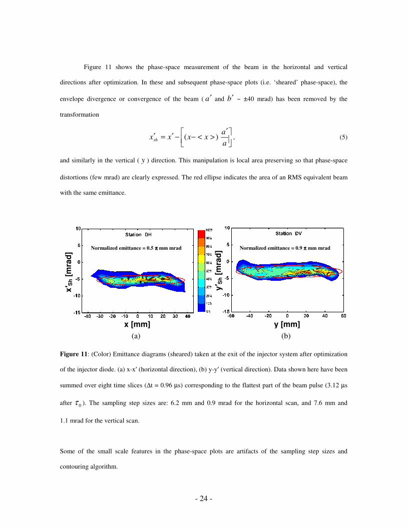
Figure 11 shows the phase-space measurement of the beam in the horizontal and vertical

directions after optimization. In these and subsequent phase-space plots (i.e. ‘sheared’ phase-space), the

envelope divergence or convergence of the beam ( a′ and b′ ~ ±40 mrad) has been removed by the

transformation

′><−−′=′

aa

xxxxsh )( , (5)

and similarly in the vertical ( y ) direction. This manipulation is local area preserving so that phase-space

distortions (few mrad) are clearly expressed. The red ellipse indicates the area of an RMS equivalent beam

with the same emittance.

Figure 11: (Color) Emittance diagrams (sheared) taken at the exit of the injector system after optimization

of the injector diode. (a) x-x (horizontal direction), (b) y-y (vertical direction). Data shown here have been

summed over eight time slices (∆t = 0.96 µs) corresponding to the flattest part of the beam pulse (3.12 µs

after 0τ ). The sampling step sizes are: 6.2 mm and 0.9 mrad for the horizontal scan, and 7.6 mm and

1.1 mrad for the vertical scan.

Some of the small scale features in the phase-space plots are artifacts of the sampling step sizes and

contouring algorithm.

Normalized emittance = 0.9 ππππ mm mrad Normalized emittance = 0.5 ππππ mm mrad

(a) (b)

yS

h [m

rad]

x [mm]

xS

h [m

rad]

y [mm]

- 25 -

The normalized emittance listed in Fig. 11 is RMSn βεε 4= , where RMSε is defined in Eq. (A2).

The injector diode retrofits decreased nε from 1.7 to 0.9 π mm mrad in the vertical direction and from 2.1

to 0.5 π mm mrad in the horizontal direction. The theoretical minimum emittance based on the emitter size

(radius = R ) and temperature (T 1100°C) is

mkT

Rn 2=ε = 0.18 π mm mrad.

Note that in Fig. 11, the ordinate ranges are the same for both plots, though the centers are shifted.

The injector beam characterization measurements and the first measurements through the HCX

were made using a contact ionization source. We switched to an improved alumino-silicate source [50], to

avoid the rapid depletion associated with doped contact ionization sources.

4. MATCHING SECTION

The matching section compresses the beam area transversely by a factor of 25 and produces the

matched beam envelope parameters a , a′ , b and b′ necessary for transport in the periodic electrostatic

lattice. In this significant beam manipulation, the maximum envelope excursions occur in the first and

second quadrupoles, filling up to 80% of the clear aperture there. Figure 12 is an example of the result from

an envelope calculation using hard-edge quadrupoles to model the focusing fields.

- 26 -

Figure 12: (Color) Representative envelope calculation of the beam going through the matching section

(for the 60% fill factor case in the downstream lattice). The red lines represent the quadrupoles’ bore radii.

Typically, the beam centroid exiting the injector is offset from the beam line axis by

1-2 millimeters and 3-5 milliradians. The centroid undergoes betatron oscillations through the quadrupoles

of the matching section. The centroid at QD1 is centered by mechanical translation of the three steering

quadrupoles QM4-6 in the matching section. The required displacements are determined by calculating the

single particle motion through these quadrupoles, and then solving for the quadrupole displacements

needed to center the beam. By this procedure, the beam centroid positions ( >< x , >< y ) and angles

( >′< x , >′< y ) are centered to within 0.5 mm and 2 mrad respectively.

Even though the beam fills a relatively large fraction of the aperture (up to 80%) in the early part

of the matching section, pickup signals capacitively connected to the quadrupole electrodes indicate that

beam loss is minimal through the middle, or ‘flattop’ of the beam pulse. This is illustrated in Fig. 13 where

the capacitive monitor waveforms for QM1 (Fig. 13(a)) and QM6 (Fig. 13(b)) positive electrodes are

plotted. The positive and negative peaks at the head and the tail of the pulse respectively are characteristic

of the rising and falling image charges of the beam induced onto the quadrupole electrodes when it enters

0

1

2

3

4

5

6

7

8

9

0 100 200 300 400

Axial Position [cm]

2*RMS B

eam rad

ius [cm]

vertical horizontal QD1

QM1

QM2 QM3

QM4

QM5

QM6

2*R

MS

Bea

m r

adiu

s [c

m]

- 27 -

and exits the quadrupole. As a check of the interpretation of the electrode monitor signals, we derived the

expected capacitive waveform based on the upstream total beam current diagnostic using Eq. (2) and added

it to Fig. 13. The good agreement with the electrode monitors for the head of the beam (see Fig. 13) shows

that the monitor signals in the matching section are from the capacitive pickup of the passage of the beam

through the quadrupole, except for the very end of the beam pulse, which will be discussed below.

- 28 -

Figure 13: (Color) Electrode monitors for the first (a) and last (b) electrostatic quadrupoles of the matching

section. The blue curve is the raw signal across 10 Ω. The dashed red curve is the expected signal derived

from a current transformer waveform at the injector exit using Eq. (2). Note that the difference in peak

amplitude for the head of the beam in the signals collected in QM1 and QM6 is due to the fact that QM6 is

QM1 electrode monitor (positive)

-1

-0.8

-0.6

-0.4

-0.2

0

0.2

0.4

0.6

0.8

2 3 4 5 6 7 8 9 10

Time [µµµµs]

Am

plitu

de [V

]

TheoryData

QM6 electrode monitor (positive)

-1.75

-1.50

-1.25

-1.00

-0.75

-0.50

-0.25

0.00

0.25

0.50

2 3 4 5 6 7 8 9 10

Time [µµµµs]

Am

plitu

de [V

]

TheoryData

(a)

(b)

- 29 -

30% shorter than QM1 and therefore the total charge subtended by the electrodes is proportionally lower in

QM6.

In Fig. 13, the collected signal in the flattop region of the pulse (between the peaks) is very small.

Following the discussion from Sec. 2.D., based on the sum of all six matching section quadrupole pickup

signals, we conclude that the beam loss is < 0.5 % of the total beam current. Because of the slow fall time

of the beam pulse, the tail is mismatched and the beam loss is greater there, as indicated by the large

negative spike on the QM6 capacitive monitor waveform (Fig. 13). The strong negative peaks at the tail are

attributed to the beam striking the quadrupoles.

The desired envelope parameters at the exit of the matching section were achieved by fitting the

envelope model described by Eqs. (3) to data. However, this model does not include effects such as fringe

fields, the Ez component of the focusing fields, image forces and the evolution of the emittance. Thus,

reaching a reasonable agreement between the measured envelope parameters and the targeted ones requires

several iterations. In order to reduce the number of iterations and have a better theoretical understanding of

the beam dynamics in the matching section, an improved model of the matching section that includes the

effects mentioned above is being developed. Nevertheless, after 3-4 iterations, the matching procedure just

described determines the required quadrupole voltages such that the envelope parameters at the exit of the

matching section are routinely to within 0.4 mm and 2.1 mrad (1σ) of the ideal matched parameters.

The horizontal phase space of the beam measured at QD1 (sheared) is shown in Fig. 14 (top row)

for the two fill factor measurements made so far (60% and 80%).

- 30 -

Figure 14: (Color) Horizontal phase-space diagrams before (top) and after (bottom) the electrostatic

transport section for (a) 60% fill factor; (b) 80% fill factor, for time slice tA (in Fig.16). For the 60% fill

factor, the sampling step sizes are: 1.5 mm and 2.3 mrad at QD1 and 1.4 mm and 2.2 mrad at D2. For the

80% fill factor, the sampling intervals are: 2.1 mm and 1.9 mrad at QD1 and 1.9 mm and 1.8 mrad at D2.

From the variance among more than 10 independent data sets at the diagnostics stations at the entrance and

exit of the transport section and slightly different lattice gradients (i.e. various quadrupole voltage solutions

in the matching and transport sections that resulted in the beam filling 60% or 80% of the clear aperture),

the estimated emittance measurement uncertainty is 10% (1σ). Though the phase-space distribution appears

more distorted for the 60% fill factor case than for the 80% fill factor case, the normalized emittance is

nearly independent of the matching solution within the experimental uncertainties. However, the beam

emittance measured at the exit of the matching section appears to be lower than the one measured at the

εεεεn = 0.40 ππππ.mm.mrad εεεεn = 0.48 ππππ.mm.mrad

εεεεn = 0.40 ππππ.mm.mrad εεεεn = 0.48 ππππ.mm.mrad

(a) (b)

- 31 -

exit of the injector (by 2.0-2.4 times in the vertical plane and, 1.0-1.2 times in the horizontal plane, for the

60% and 80% fill factor cases, respectively, Fig. 11). Since a sub-percent beam loss can not account for

such a large discrepancy, these differences point to a large overestimation of the emittance measurements

made at the exit of the injector due to systematic instrumental errors. There are three effects: the finite

width of the slits, the misalignment of the slits with respect to one another (i.e. slit and slit-cup not exactly

parallel to one another), and the rotation of the beam principal axis with respect to the main axis of the

transport channel (horizontal and vertical, on which the slits are aligned). The errors due to finite slit width

account for 1% increase in the perceived emittance for all measurements. Both alignment effects increase

the apparent beam emittance, and are pronounced when the beam is large ( a 40 mm and b 60 mm as

at the injector exit) and are negligible when the beam has been transversely compressed by the matching

section ( a 10 mm, b 15 mm). A Monte-Carlo simulation of particles followed through the emittance

scanner shows that the larger emittance at the injector exit may be explained by a transverse beam

rotational misalignment of 1.5° plus the slit and slit-cup misaligned by 0.25 mrad. Additionally, 3D PIC

simulations of the HCX experiment indicate that the emittance should (initialized with a semi-Gaussian

distribution at the matching section entrance) remain constant in the matching process or increase by 1.3

times (simulations started at the ion emitter surface) [11].

Furthermore, the measured emittance depends on the sampling step size of the measurements.

Increasing or decreasing the step size by a factor of two contributes to a 2% difference in the calculation

of the emittance, based on linear interpolations of the data.

The uncertainties for the beam envelope parameters were characterized by calculating the standard

deviation (1σ) of five repeated measurements, where the data were summed over a 1.5 µs window near the

flat top region of the beam current pulse. By this measure, the stability and reproducibility of the envelope

coordinate ( a , b ) and angle ( a′ , b′ ) measurements are 0.3 mm and 1 mrad, respectively, which

includes the effect of the beam current drift over the course of the measurement (~1 hour) of up to 2 mA

out of a nominal beam current of 183 mA.

5. BEAM CURRENT TIME DEPENDENCE STUDY

- 32 -

The head and the tail of the beam pulse, where the current rises or falls through 0-95% of the

maximum, have very large systematic variation in envelope parameters, inevitably leading to envelope

mismatches. But, partly because of the lower beam current, we find that for the head the envelope can

remain confined with negligible beam loss. However, even in mid-pulse, as much as 50% variations in

beam size and angle were observed at QD1 (for a 60% fill factor solution) when the beam current varied by

~15% in early measurements (Fig. 16). The time dependence of the envelope parameters emerging from the

matching section is driven by variations in the extraction voltage which controls most of the emission (and

therefore the beam current) at the beginning of the injector. The downstream trajectories in the injector

differ greatly with current when the extraction voltage varies independently of the Marx voltage. This is in

contrast to the situation where all the injector voltages are scaled together and the trajectories are identical.

Such sensitivities were predicted by 3D PIC simulations of the injector followed with envelope simulations

through the matching section.

The strong correlation between beam current and envelope parameters is illustrated in Figs. 15 and

16, which show measured current waveforms and the corresponding measured envelope parameters, b and

b′ , before and after extraction voltage waveform tuning, for which the time dependence is significantly

different. A time slice, tA, at which the beam current waveforms at the different times intersect (Fig. 15) is

identified. The corresponding time slice at QD1 (Fig. 16) is also identified. Note that the measured

envelope parameters at this time slice intersect to within the measurement uncertainties.

- 33 -

0

25

50

75

100

125

150

175

200

1.0 2.0 3.0 4.0 5.0 6.0 7.0 8.0 9.0 10.0 11.0 12.0Time [µµµµs]

Bea

m c

urre

nt [m

A]

Before Vgate tuning After final Vgate tuning

tA

trise (10-90%) = 250 ns

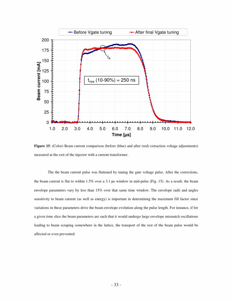
Figure 15: (Color) Beam current comparison (before (blue) and after (red) extraction voltage adjustments)

measured at the exit of the injector with a current transformer.

The the beam current pulse was flattened by tuning the gate voltage pulse. After the corrections,

the beam current is flat to within 1.5% over a 3.1 µs window in mid-pulse (Fig. 15). As a result, the beam

envelope parameters vary by less than 15% over that same time window. The envelope radii and angles

sensitivity to beam current (as well as energy) is important in determining the maximum fill factor since

variations in these parameters drive the beam envelope evolution along the pulse length. For instance, if for

a given time slice the beam parameters are such that it would undergo large envelope mismatch oscillations

leading to beam scraping somewhere in the lattice, the transport of the rest of the beam pulse would be

affected or even prevented.

- 34 -

10.0

12.0

14.0

16.0

18.0

20.0

22.0

24.0

26.0

5.0 5.5 6.0 6.5 7.0 7.5 8.0 8.5 9.0Time [µµµµs]

Bea

m s

ize

[mm

]

20.0

25.0

30.0

35.0

40.0

45.0

50.0

55.0

60.0

Bea

m a

ngle

[mra

d]

b (before Vgate tuning) b (after Vgate tuning)

b' (before Vgate tuning) b' (after Vgate tuning)

tA

Figure 16: (Color) Vertical envelope parameters ( b (dark and light blue curves) and b′ (red and orange

curves)) at QD1 diagnostics station as a function of time before and after the extractor voltage adjustments.

6. TRANSPORT THROUGH ELECTROSTATIC QUADRUPOLES

Ideally, the fill factor experiment would be done using constant current density beams of various

sizes, for which 2aI B ∝ and the interior trajectories are self-similar. We chose to vary the tune and

matching to achieve various fill factors, but at varying current densities. Alternative techniques such as the

use of apertures and making several ion sources of different sizes were deemed too complicated or too

expensive. In particular, the beam aperturing process can induce significant undesirable complications (e.g.:

desorbed gas and secondary electrons production) that may distort the beam in the transport section. PIC

simulations of the experiment in which various fill factors were achieved either at fixed current density or

by varying the quadrupole tune gave similar results [45], giving confidence that the experimental approach

- 35 -

(i.e. exploring the fill factor by decreasing the lattice focusing strength) will give information relevant to

the driver case.

We have made two fill-factor measurements, for the envelope filling 60% and 80% of the

available bore diameter in the transport channel of 10 electrostatic quadrupoles arranged in a periodic

lattice. For each fill factor measurement, the transverse phase space of the beam was characterized in detail

at the exit of the matching section, as discussed in Sec. 4. Each case required a different matching solution

(i.e. different quadrupole voltages in the matching section). Because the fill factor was changed by tuning

the upstream beam to the matched beam conditions in the transport section for a lower focusing gradient,

rather than by changing the current, the undepressed betatron phase advances per lattice period (σ0) for the

two fill factors are different (69° and 48° for the 60% and 80% fill factor cases, respectively). The

depressed phase advances per lattice period (σ) due to the self potential of the beam are 13° and 8° for the

60% and 80% fill factor cases, respectively.

Similar to the matching section results, in the entire length of the electrostatic transport section,

considering the mid-pulse and both fill factor cases, beam loss is 1%. This is based on the sum of the

currents collected on all 10 quadrupole electrodes interpreted per Sec. 2.D., which indicate particle loss of

< 1% and the ratio of Faraday cup currents at the entrance and exit of the transport section indicating 1%

loss.

Figure 17 shows quadrupole electrode pick-up signals for 80% fill factor measurements. Because

the pickup signals at the head and tail of the beam are the result of a combination of both the capacitive

response and the collected currents, it is difficult to interpret.

- 36 -

Figure 17: (Color) Electrode monitors for the first (blue) and last (brown) electrostatic quadrupoles of the

transport section for an 80% fill factor case. In red is the sum of all 10 quadrupole pick-up signals in the

middle of the beam pulse. This sum is representative of the beam loss through scraping and

beam/background gas interactions.

Moreover, because of the intrinsic mismatch of the head and tail of the beam, the individual electrode

monitor signals amplitude is smaller or in some instances negative at the beginning of the pulse and is more

negative at the end of the pulse, indicating more beam loss at the extremities of the pulse.

From Fig. 14, it can be seen that within the experimental sensitivity, there is no evidence of

emittance growth at the end of the electrostatic lattice for both the 60% and 80% fill factors in the

horizontal plane. This result is also true for the vertical direction (diverging plane). Note also that the

details of the beam phase-space distribution remain practically unchanged except for the small ‘hooking’

regions that mirror one another between QD1 and D2. PIC simulations initialized with semi-Gaussian

distributions [8,45] have also predicted that matched beam excursions filling 80% of the quadrupole bore

would result in negligible emittance growth, assuming perfect alignment and envelope control. However,

these simulations do not include nonideal effects resulting from particle losses. To date, comparisons of

measured phase-space distributions to PIC simulations show that the measured distributions are not well

-1.4

-1.2

-1.0

-0.8

-0.6

-0.4

-0.2

0.0

0.2

0.4

-1 0 1 2 3 4 5 6 7 8 9 10

Time [µµµµs]

Am

plitu

de [V

]

QD1

QI10

Sum ofsignals

- 37 -

reproduced in the theoretical model, even when initialized with a distribution reconstructed from the data

(see Sec. 7). Note that in Fig. 14, the signal-to-noise ratio for the QD1 data sets is 5× larger than for the

D2 data sets.

Integrating the envelope equation from QD1 to D2 (initialized with QD1 measurements of

envelope radii, convergence angles, current, and measurements of beam energy) gives a calculated

envelope in agreement with the experiment at the D2 location to within 0.4 mm and 3 mrad. This level of

agreement allows us to confidently rely on envelope model predictions (such as Fig. 18) to tune the lattice

and control the beam envelope excursions in the experiment. Early calculations of the envelope showed

discrepancies as large as 25%. After including the following effects in the theoretical model, as well as a

more accurate determination of the beam current, the beam energy and the variation of the beam parameters

over the pulse, the agreement was good as indicated above. The improvements to the model were: (1)

Realistic quadrupole fringe fields based on 3D field calculations; (2) quadrupole Ez from the 3D lattice

structure and corresponding radial focusing force; (3) corrections due to the grounded slit plates of the

intercepting diagnostics that short out the self-field of the beam near the diagnostic [9]. In Fig. 18,

examples of calculated beam envelopes with these improvements are plotted. In Table II, envelope

measurements at the exit of the electrostatic lattice for two 80% fill factor data sets are compared to

predictions of the envelope model. Envelope simulation uncertainties are taken from the standard deviation

of a Monte Carlo distribution of envelope predictions through the transport section, where several thousand

of envelopes are calculated with initial conditions randomly distributed about the measured values. The

initial distributions for the parameters that are varied are Gaussian with standard deviations representing the

measurements uncertainties or the equipment accuracies (e.g.: stability of the quadrupole voltages)

previously discussed.

- 38 -

Figure 18: (Color) Calculated envelope from QD1 to D2 for (a) a 60% fill factor case; (b) a 80% fill factor

case. Runs are initialized with data taken at QD1. Black: horizontal direction; Red: vertical direction; Green:

focusing forces quadrupole gradients.

The uncertainties for the data at D2 are estimated as for the QD1 uncertainties described in Sec. 4.

Thus, the RMS envelope model is accurate to within the measurement uncertainty.

(a) (b)

- 39 -

Table II: Experimental envelope parameters compared to envelope model predictions at the exit of the

electrostatic section for two 80% fill factor cases. Note that in this table, data sets A and B were taken at

different z locations in the lattice, as pointed out in Sec. 2.D. The data are from a 120 ns interval of the

flattop region of the beam pulse, 2.64 µs after 0τ .

a a b b

[mm] [mrad] [mm] [mrad]

Experiment 12.24 -38.52 21.10 43.04 Data set A

Env. Model 12.07 -35.46 20.95 46.10

Experiment 14.07 -38.50 15.54 39.84 Data set B

Env. Model 14.66 -38.05 15.13 38.10

Experiment 0.3 1.0 0.3 1.0 Uncertainty (±1σ) Env. Model. 0.5 2.1 1.2 3.0

Further data analysis shows that RMS beam parameters are more sensitive to beam current

variations for a 60% fill factor case than for an 80% fill factor case.

Defining the envelope mismatch as MaxMaxMaxM RbaMax ,0),( −=δ , where

),( MaxMax baMax is the maximum of the envelope excursions in both planes of the calculated envelope

initialized with QD1 measurements, and MaxR ,0 is the maximum excursion for the theoretical matched

beam, for both fill factor cases shown on Fig. 18, we were able to match the beam to within

Mδ = 1 ±0.5 mm. The uncertainty in Mδ is based on the Monte Carlo analysis discussed above.

Envelope simulations for which the quadrupole voltages were allowed to vary randomly by the

expected tolerance on voltage control (0.1 kV or 0.5%) about their nominal value, including the

experimental constraint that five of the 10 quadrupoles are energized with common power supplies,

indicate that the average envelope mismatch excursion grows by 0.2-0.3 mm over the first five lattice

periods. This rate decreases to less than 0.1 mm per five lattice periods after transport through 50 lattice

periods.

- 40 -

With the beam centered to within 0.5 mm and 2 mrad upstream (QD1), we observe

1-2 millimeters and 1-5 milliradians centroid offsets after these 10 quadrupoles and the beam centroid

varies by 0.5 mm and 1 mrad during the flat top of the beam pulse. However, the predicted centroid

values from simulations do not agree with the downstream beam measurements. The quadrupoles were

aligned with respect to their common support rail to within ±100 µm. There is no common misalignment of

the quadrupole support rail that satisfies all the data sets. Dipole fields from image charges in the 10

transport quadrupoles or induced by the image charge of the beam on the support slit scanner paddles in the

relatively open diagnostic regions may be responsible for the discrepancy. However, it was observed that

upstream (QD1) beam centroid offsets as large as 2 mm and 5 mrad would not lead to any noticeable beam

loss or emittance growth in the electrostatic transport section.

7. BEAM CHARGE DISTRIBUTION

From crossed slit measurements (i.e. perpendicular slits upstream of a Faraday cup, each sampling

the beam distribution in x∆ = y∆ = 1 mm intervals) at QD1 and D2, the time-resolved current density

distribution ),,( tyxJ (see Fig. 19) of the beam was measured. Depending on the applied focusing

strength in the matching and transport sections, J may be peaked or hollow in radial profile. The initial

nonuniformities in the current density distribution arise from the diode spherical aberrations [5]. Also, the

shape of the transverse beam profile exhibits diamond-like distortions from ideal elliptical symmetry at

both diagnostics stations. Transverse oscillation frequencies (e.g. plasma, space charge wave and envelope

oscillations frequencies) are influenced by the change in σ0 associated with the two fill-factor

measurements. As a result, different current density distributions were observed.

- 41 -

Figure 19: (Color) Beam current density profiles ),( yxJ measured with crossed slits. (a) - (b): 60% fill

factor case at QD1 and D2 respectively, single time slice (∆t = 0.12 µs) taken 2.64 µs after 0τ (c) - (d):

80% fill factor case at QD1 and D2 respectively, single time slice (∆t = 0.12 µs) taken 3.12 µs after 0τ . In

(b) and (d) the dark crossed (or line) pattern that is seen comes from bridges across the slits that are there to

strengthen the slit structure and avoid deformations.

The diamond-shaped pattern is attributed to nonlinear fields arising from the space charge

component of the distribution and the collective evolution of the distribution in the ESQ injector and in the

matching and transport sections. The fact that the 60% fill-factor beam, though having smaller radius, is

more diamond-shaped than the 80% fill-factor beam indicates that nonlinearities from the image forces and

the applied fields in the transport section do not play a significant role. Most of the distortion is initiated

upstream, in the injector and matching section.

(a) (c)

(b) (d)

x [mm] x [mm]

x [mm] x [mm]

y [m

m]

y [m

m]

y [m

m]

y [m

m]

- 42 -

Simulations [71] indicate that the peaked and hollow patterns are due to transverse space-charge

waves that move rapidly in and out of the body of the beam (From Ref. [22,25] ωspace charge wave > ωplasma for

all modes). Therefore, the details of the beam current density distribution vary with the longitudinal

position in the lattice.

The ),( yxJ data are used with the phase space data at QD1 to construct a consistent particle

distribution for simulation studies [11].

Figure 20: (Color) Beam current density profiles ),( yxJ at mid-pulse (2.64 µs after 0τ ) (a) data at D2,

(b) WARP simulation at D2 initialized with data at QD1, projected to a common plane in the lattice. Spatial

hollowing in the center of the beam distribution is a common feature to both the data and simulation.

x [m]

y [m

] y

[m]

x [m]

(a)

(b)

- 43 -

Figure 20 shows the first PIC simulations of the beam initialized with a distribution reconstructed from

measurements of the 60% fill-factor case at QD1. The simulation uses 2 x 105 particles on a 0.2 mm grid

and the focusing fields were obtained from a multipole decomposition of the calculated electrostatic field

based on the mechanical design of the HCX quadrupoles.

Both the simulated and measured beam configuration space distributions are hollow (center to

edge: 1:2) but the distributions are different. However, second order parameters such as the RMS beam

size and convergence/divergence angles differ significantly between the experiment and the simulation.

Several items contribute to the disagreement: First, the reconstruction algorithm (still under development)

does not exactly reproduce the initial measured second moments of the beam at QD1. In particular, a′ and

b′ differ from the experiment by 1 mrad. Then, the beam energy for this data set is not known to better

than 5 to 10%. Combined, these two sources of error could account for as much as 10 mrad and 2 mm

differences in the beam envelope parameters expected at D2. Another effect which is not yet taken into

account in PIC calculations, is the beam self-electric field shorting out by the measuring slit [9]. Envelope

calculations including this effect show that it contributes to another 0.5 mrad difference to the final beam

envelope angles expected at D2. Finally, the measurement of the 4-D phase space with the standard slit/cup

diagnostics is incomplete, since only the xx ′− , yy ′− and yx − projections are measured. In order to

realistically describe the detailed evolution of the beam distribution, the full 4-D phase-space needs to be

known, since cross correlations exist between the vertical and horizontal projections

[ ),,( tyxf ′ , ),,( txyf ′ and ),,( tyxf ′′ ]. A new optical diagnostic (discussed in Sec. II.D.) measures

the missing projections of the 4-D phase-space distribution and will improve our ability to simulate

accurately the beam throughout its transport in the electrostatic section and beyond.

The time-resolved crossed-slit data show that at QD1 the profile of the beam during the rise and

fall of the beam current pulse and for both fill factors is larger than during the flattop (Fig. 21).

- 44 -

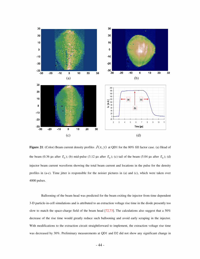
Figure 21: (Color) Beam current density profiles ),( yxJ at QD1 for the 80% fill factor case. (a) Head of

the beam (0.36 µs after 0τ ); (b) mid-pulse (3.12 µs after 0τ ); (c) tail of the beam (5.04 µs after 0τ ); (d)

injector beam current waveform showing the total beam current and locations in the pulse for the density

profiles in (a-c). Time jitter is responsible for the noisier pictures in (a) and (c), which were taken over

4000 pulses.

Ballooning of the beam head was predicted for the beam exiting the injector from time dependent

3-D particle-in-cell simulations and is attributed to an extraction voltage rise time in the diode presently too

slow to match the space-charge field of the beam head [72,73]. The calculations also suggest that a 50%

decrease of the rise time would greatly reduce such ballooning and avoid early scraping in the injector.

With modifications to the extraction circuit straightforward to implement, the extraction voltage rise time

was decreased by 30%. Preliminary measurements at QD1 and D2 did not show any significant change in

(a) (b)

(c) (d)

-200

20406080

100120140160180200

2 3 4 5 6 7 8 9 10 11

Time [µµµµs]

IB [

mA

] (a)

(b)

(c)

- 45 -

the RMS beam parameters in the beam head at the exit of the electrostatic transport section. However, it is

possible that the effect of the faster rise time on the beam envelope is obscured by the large compression

and mismatch of the head through the matching section, for instance if the head scrapes early in the lattice.

Calculations of the head-tail dynamics through the rest of the HCX are underway.

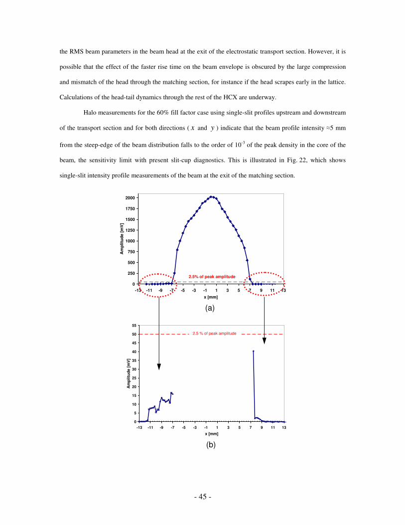
Halo measurements for the 60% fill factor case using single-slit profiles upstream and downstream

of the transport section and for both directions ( x and y ) indicate that the beam profile intensity 5 mm

from the steep-edge of the beam distribution falls to the order of 10-3 of the peak density in the core of the

beam, the sensitivity limit with present slit-cup diagnostics. This is illustrated in Fig. 22, which shows

single-slit intensity profile measurements of the beam at the exit of the matching section.

0

250

500

750

1000

1250

1500

1750

2000

-13 -11 -9 -7 -5 -3 -1 1 3 5 7 9 11 13

x [mm]

Am

plitu

de [m

V]

2.5% of peak amplitude

0

5

10

15

20

25

30

35

40

45

50

55

-13 -11 -9 -7 -5 -3 -1 1 3 5 7 9 11 13

x [mm]

Am

plitu

de [m

V]

2.5 % of peak amplitude

(a)

(b)

- 46 -

Figure 22: (Color) Single slit profile measurements showing the extent of the halo and our present

diagnostics’ sensitivity for a 60% fill factor case at QD1 (horizontal direction). (a) is a typical whole beam

profile; (b) are partial profiles (acquired close to the beam edges only) with 100x greater gain on the

oscilloscope. Error bars are smaller than the plot points.

8. ABSOLUTE BEAM ENERGY MEASUREMENTS

Two new diagnostics, an electrostatic energy analyzer (EA) and a time-of-flight pulser (TOF) (see

Sec. 2.D.) were installed to more precisely determine the beam energy and for longitudinal phase-space

measurements, though the energy resolution is not small enough to resolve the temperature component.

Figure 23 shows the longitudinal energy distribution obtained with the EA. The 10%-higher

energy head and long low-energy tail are a combined effect of longitudinal space charge, which accelerates

particles at the front end of the pulse and decelerates particles at the rear of the pulse, and the extraction

voltage pulse shape. In particular the slow fall time of the extraction voltage pulse causes the tail energy

variation to be twice as great as the variation of the head. These data also show that in the middle of the

pulse, the mean beam energy, <EB>, is constant to within 0.5% for 3.1 µs.

- 47 -

Figure 23: (Color) Longitudinal energy distribution measured with the electrostatic energy analyzer. K+

ions were detected at the beam head with 1.1 MeV (not visible on this scale).

Figure 24 shows the perturbation produced by the TOF pulser on the beam current waveform, as

measured downstream, along with a theoretical calculation of the expected perturbation based on a 1-D

cold-fluid model [16]. Because of our relatively short beam line, the peaks of the forward- and backward-

traveling waves have not yet clearly separated. The energy perturbation is applied by raising the potential

of the first matching section quadrupole with respect to its neighbors, which induces a perturbation in the

gaps preceding and following the quadrupole, each perturbation resulting in two waves that propagate in

opposite directions. These four waves interact with one another while traveling down the beam line, adding

some complexity to the observed current waveform perturbation downstream.

- 48 -

Figure 24: (Color) Cold fluid model vs. measurement of the perturbation on the beam current waveform.

Initial perturbation applied at t = 0. The beam energy is the only fitted parameter for the cold-fluid model.

The upstream voltage pulse waveform and pulsed quadrupole length was input to the model calculation.

The beam energy is determined by fitting the model to the data using the beam energy as the only

independent parameter.

The TOF and EA diagnostics both determine the absolute beam mean energy to ±2%, with both

measurement methods agreeing within these uncertainties (Fig. 25). Errors for the EA measurements

mostly arise from the calibration procedure (uncertainty of the hole-plate bias voltage and of the fitted K2+

ion energy change due to the bias). The dominant source of error for the TOF measurements is determined

by the fit between the model and the data. Other errors include the determination of the distance between

the z location of the kicker and the measuring plane, the timing of the cables and the time at which the

perturbation is applied.

-0.08

-0.04

0

0.04

0.08

2 2.4 2.8 3.2

Time of flight [µµµµs]

Rel

ativ

e A

mpl

itude

Theory Experimental Data

- 49 -

Figure 25: (Color) Comparison between the Time of Flight and the Energy Analyzer measurements of the

beam mean energy. In blue and red are the results from the TOF measurements. In green is the result of the

energy analyzer measurement.

Before these measurements, the beam mean energy was estimated to be 1045 keV, based on the

calibration of the capacitive probe that monitors the Marx voltage near the HV dome. This calibration is

performed at low voltage and at atmospheric pressure in the dome, in a geometric configuration slightly

different from normal operation. From the energy analyzer, the beam mean energy is 962 keV (±2%),

almost 10% lower than determined by the capacitive probe. These measurements then provide an

independent calibration of the capacitive probe, which monitors the injector voltage on every shot. The

precise determination of the energy is essential for the agreement between envelope simulations and

experimental data in Sec. 6 and 7. For example, a 2% energy variation at the injector exit induces as much

as 20% beam size variation in the vertical direction at the matching section exit.

930

950

970

990

5.5 6.5 7.5 8.5 9.5

Time [µµµµs]

<E>

[keV

]

TOF data (Slit/cup) TOF data (large Faraday cup)Energy Analyzer data

- 50 -

9. DISCUSSION

In the electrostatic transport section, the data agree well with envelope calculations that include

realistic fringe fields and the effects of the intercepting diagnostics. Additionally, the relative sensitivity to

beam current variations shown in the 60% fill factor data versus the 80% fill factor data is understood in

terms of envelope mismatch oscillations, which arise when one or more of the terms in the envelope

equation is perturbed (i.e. small variations around the ‘matched beam’ conditions) [16,52]. In an AG lattice,

envelope oscillations can be decomposed into the combination of two fundamental modes equivalent to the

breathing and quadrupole modes derived from a continuous focusing analysis, but at slightly different

characteristic frequencies [16]. Using an envelope model in which the beam current is varied for otherwise

matched parameters, Fourier transforms of the calculated envelope suggests that the current perturbations

excite the breathing mode more strongly compared to the quadrupole mode. For the 80% fill factor case,

where the undepressed phase advance per lattice period, σ0, is 48°, the total phase advance of the breathing

mode envelope oscillation through 10 quadrupoles (i.e. 5 lattice periods) is 360°. Thus, the envelope

parameters should show a reduced sensitivity to small beam current variations, in line with the observations.

The improved envelope model will improve our ability to manipulate the beam envelope for further

experiments, such as launching almost pure envelope mismatch modes (quadrupole or breathing), and to

predict the proximity of the 2 RMS beam edge to the bore aperture. The agreement between model and

experiment supports the expectation that electrons are promptly swept out of the path of the beam by the

focusing electric fields.

Beam steering using 2-3 movable quadrupoles, which requires a good knowledge of the focusing

fields and relative displacements of the quadrupoles, is successful at re-centering the beam. However, the

predictions of the beam centroid trajectory over the length of the transport section, which requires absolute

measurements of misalignments of the focusing elements and diagnostics with respect to the system center

line, are not as accurate ( 3 mm, 6 mrad) as the predictions of the envelope parameters (< 0.5 mm,

3 mrad). Image charges and stray dipole due to asymmetric boundary conditions at the diagnostics while

acquiring the data may explain this discrepancy. Transport lattices for HIF will have centroid corrections

- 51 -

periodically. Understanding the accumulation of centroid errors is important for determining the frequency

of correction elements.

The time dependence of beam parameters is also important when defining the limit of the

transportable current. The envelope variations throughout the beam pulse inherently lead to a mismatch that

can be severe. The time-dependence of the beam parameters near the head of the beam pulse shows that the

injector waveform rise time is critical for beam matching since this manipulation involves rapid envelope

transitions and could easily deteriorate the beam pulse uniformity (as a function of time) at the beginning of

the accelerator. Time-dependent focusing gradients to match the beam head might be possible depending

on required specifications and cost. At the head of the beam pulse, size and angle mismatch may disrupt the

propagation of the rest of the pulse, especially in magnetic focusing transport channels secondary electrons

may be trapped in the rising beam potential. Aperturing the beam in order to scrape off the beam head must

be done at a few lattice locations where the envelope excursion of the beam head is relatively large, and

may be implemented in future experiments. The ‘ballooning’ of the head is minimized when the extraction

pulse waveform is tailored such that its rise time matches the space-charge field buildup at the emitter [72].

Also, from halo scrape-off at the head and flattop of the beam, gas atoms from the wall are

released. The gas atoms will intercept the beam path and induce further loss depending on the atom

velocity, the beam-edge to wall clearance and the pulse length.

The velocity tilt for pulse compression at the beginning of a fusion driver in an electrostatic

quadrupole transport channel results in a beam whose transverse size increases throughout the pulse

(smaller head, bigger tail) while its length remains constant. Although WARP simulations show that during

this manipulation the beam remains nearly matched for all time slices, one must take into account these

variations in envelope excursion throughout the beam pulse when assessing the acceptable fill factor, and

allow for a range of envelope sizes.

The injected beam is non-uniform in current density as a function of x and y , and remains so for

the length of the present beam line as shown by current density measurements at D2 (Sec. 7). The non-

uniform distribution induces transverse space-charge waves that oscillate as the beam propagates. The

current density distribution differences seen at the exit of the electrostatic transport section between the two

fill factor measurements can be explained qualitatively using a warm-fluid description of an intense beam

- 52 -

equilibrium [22] and are also consistent with a full kinetic treatment for an AG lattice as calculated by

Hofmann et al. [25]. Although the theory is developed for small amplitude perturbations in axisymmetric

geometry, it appears to have predictive power in our non-ideal context. In this context, the normalized

frequency 0ν

ω of axisymmetric flute perturbations as a function of the tune depression

0νν

for a K-V

beam equilibrium in the electrostatic approximation is given by the dispersion relation [22]

( )1222 2

2

0

2

0

−

+=

n

νν

νω

, (6)

where n is the radial mode of the perturbation, which radial profile can be described by a series expansion

of Legendre polynomials of degree n ,

LvBσν = (7a)

and

LvB

00 σν = (7b)

the depressed and un-depressed betatron frequencies, with Bv being the ion velocity and L the lattice

period. Since for both fill factor cases the beam distribution at QD1 is peaked (Fig. 19(a, c)), we define

these measurements to represent the initial perturbation of the density profile (mainly to a radial 2=n

mode; a fuller description of the perturbation is composed of additional higher order eigenmodes). Then,

the difference in the density profiles at the exit of the transport section (D2) is interpreted as the difference

in the phase of the perturbation. At respective tune depressions 0ν

ν = 0.19 and 0.16 for the 60% and 80%

fill-factor cases, the phase difference expected at D2 (five lattice periods downstream) is ∆φ = 167 degrees.

Since the beam distribution started peaked at QD1 for both cases, we expect the distribution to be almost

completely out of phase at D2 (Fig. 19(b, d)). An additional 20-30 quadrupoles would increase the transport

length to 4.5-6 times (2πν/ωp) plasma periods and theoretical models predict that this would be just enough

- 53 -

for the space-charge waves to phase mix, eliminating most of the phase space and distribution

inhomogeneities [8,11,15].

Crossed-slit current density profile data prompted a comparison to an idealized thermal

equilibrium distribution using the Vlasov equation, which showed that the equivalent thermal distribution

profile falls rapidly at the beam edge in 5 Debye lengths (95 to 5%), yxD ,λ , outside a near-constant density

core, with

aKb

b

xDx 222 γ

ελ = , (8a)

bKa

b

yDy 222 γ

ελ = , (8b)

where bγ = 1 is the Lorentz factor of the beam. For the HCX beam parameters, Dxλ 0.8-0.9 mm (80%-

60% fill factor) and Dyλ 0.4-0.7 mm (60%-80% fill factor). Thus, the rate of fall-off calculated is in

reasonable agreement with the data (~2-5 mm) and measured beam emittance, though the actual beam is

not in thermal equilibrium. The beam temperature is not the same in both projection planes due to the

different beam sizes, so the model predicts that the rate of the beam edge fall-off should be steeper in the

vertical ( y ) direction (diverging, colder at all measurement planes) than in the horizontal ( x ) direction

(converging, warmer at all measurement planes). However, because of the 1 mm x and y spatial

resolution of our current density maps, the relatively small difference was not resolved. Moreover, a more

quantitative interpretation of the data requires including the effects of dynamics induced halo and space

charge waves.

Transport experiments in the magnetic quadrupole section have started, with a focus on

developing new in-situ diagnostics to measure (directly or indirectly) quantities such as the degree of beam

neutralization, the electron and neutral density and the beam potential radial distribution. Measurements in

the magnetic transport section will also have a direct impact on the design of future heavy ion induction

accelerators. In future publications, comparisons will be made between the experiments and theories of

electron dynamics in magnets [7,62]. In parallel, superconducting quadrupoles and compact cryostats are

being designed and tested [10] for similar experiments on the HCX beam line.

- 54 -

In order to develop the capability to simulate intense beams for accelerator design, details of the

measured phase space distribution are being used to initialize particle-in-cell simulations for comparison of

data with theoretical models. Prototype diagnostics with scintillator imaging show that the higher data

acquisition rates and measurement of all the correlations in the four-dimensional transverse phase-space

available with this diagnostic will enhance the theory/experiment comparison.

The measurement of the head and tail energy variations with respect to the core of the beam pulse

was used to help complete the design of a bunch end control module [24] (an induction module to correct

the energy vs. time profile of the bunch) to be installed between the matching section and the periodic

transport lattice. It is designed to correct ±20 kV waveform imperfections and also provides 100-200 kV

longitudinal focusing voltages to counteract the longitudinal space-charge field at the head and tail of the

beam. Experiments with this module will be a first step towards conducting longitudinal physics

experiments on a longer transport lattice.

Higher fill factors will also be studied. For an induction linac driver comprised of many (~100)

parallel beams that should be nearly identical, there will be additional system complexity, with some

alignment and matching issues that have not been addressed explicitly in this experiment. In the context of

multiple beam arrays for heavy-ion fusion, electrostatic quadrupoles composed of cylindrical electrodes

make a compact unit cell. For the 1-MeV beam measurements, the current density averaged over a unit cell

is <J> 40 A m-2 (denominator includes the area occupied by the beam focusing electrodes between

adjacent channels of an array), and future measurements at 1.8 MeV will increase this by a factor of 2.4, to

nearly 100 A m-2.

Designing a future linear accelerator for heavy ion fusion on the basis of the 60-80% fill factor

would constitute a significant departure from other linear accelerators, which rarely exceed 50% (at 2σ) in

order to accommodate the tail of the Gaussian beam distributions. For example the SNS linac [29,38] or

Rare Isotope Accelerator (RIA) [39,40,41] have design fill factors in the range of 30-55%, and the

maximum fill factor only occurs over short regions in the lattice. Most of a fusion driver will use magnetic

quadrupole focusing, which has increased strength at higher ion velocity than electrostatic quadrupoles.

Though the field quality of magnetic [10] and electrostatic lattices may be similar in an integrated sense,

field nonlinearities are different in spatial distribution at the lead and return ends. The useful fill factor in

- 55 -

the magnetic lattice will also be influenced by trapped secondary electrons [51], and gas desorption. The

influence of gas desorption is mitigated by shorter pulse length at higher ion kinetic energy.

There is a design trade-off between: (a) the frequency of diagnostics, steering and matching

adjustments, (b) manufacturing and alignment tolerances, and (c) fill-factor. A higher fill factor will

generally require more frequent beam adjustments. In particular, the difficulties we encountered in

controlling the beam centroid motion emphasize the importance of measuring and correcting for beam

centroid displacements. However, the 80% fill factor results together with additional observations made for

misaligned beams at the entrance of the electrostatic transport section (Sec. 6) suggest that correction

elements may only be needed every ten lattice periods (20 quads, 4.4 m). Note that the beam centroid

oscillations are driven by the applied strength of the focusing element, which in our experiment produced

0σ < 70°. A fusion driver would probably operate at σ0 80°, making it more sensitive to misalignment

errors and centroid offsets.

The calculated maximum envelope excursion is expected to grow by about 0.1 mm per five lattice

periods (Sec. 6). This result implies that, for RMS envelope control, beam re-matching is not critical for the

transport of high fill factor beams over long (50 lattice periods) distances. However, these extrapolations do

not address the magnitude of emittance growth and halo formation due to mismatch over long distances.

X. CONCLUSION

The High Current Experiment studies – at driver-relevant parameters -- the question of how much

clearance is needed to transport high-line-charge-density, high-perveance beams over long distances with

acceptable beam degradation, and from this to also refine the value of the channel size for the transport of

the maximum charge averaged over an array of beams. This is important input for the future design of a

heavy-ion fusion driver.

We successfully improved the optics of the 2-MV injector to deliver a beam compatible with the

experiments downstream, with reduced emittance and reduced phase-space distortions. While the current

density distribution remains non-ideal, the final normalized emittance is low (< 0.5 π mm mrad for 180 mA

at the exit of the matching section).

- 56 -

The achievable beam envelope and centroid control in the matching section are key ingredients in

determining the allowable fill factor in the downstream transport channel. We find that the large transverse

compression factors of the matching section result in greater sensitivity to the fringe field of the optics.

Even though it often required several iterations, the required beam control was successfully achieved, with

< 1.5 mm mismatch amplitudes in the downstream channel.

The results of transport through the first ten electrostatic quadrupoles indicate transport with a

high beam fill factor (at least 80%) is possible with negligible emittance growth and beam loss. This was

achieved in a single beam line that includes most of the uncertainties that surround the construction of a

full-scale driver (e.g.: manufacturing of components, system alignment, high voltage stability) and the

production of a high current beam (current density non-uniformities, velocity tilt, halo particles, partial

neutralization) except for the uncertainties related to an array configuration.

Accurately modeling effects such as the behavior of halo and secondary particles that result from

interactions with the wall or the background gas and the detailed beam current distribution is where present

theoretical and computational efforts are focused. While 10 or 20 quadrupoles are too few for settling

questions of emittance evolution in a long transport system, they are of the correct length for the rapid

initial evolution of the emittance and beam profile, which is expected in the front end of an accelerator.

System studies show that the cost dependence of a fusion power plant with respect to the fill factor makes

high fill factors very desirable [63]. PIC simulations initialized with a semi-Gaussian distribution indicate

that 80% might be a limit of what is achievable [8] and is near the threshold for particle loss from halo

formation.

Agreement within experimental and model uncertainties was reached between an improved

envelope model of the transport section and the data. In addition, measurements of the beam current density

distribution at the entrance and exit of the transport section and TOF measurements showed good

agreement with simple theories describing the transverse and longitudinal evolution of the space-charge of

the beam, respectively (i.e. space-charge waves).

Image charge forces in the transport section do not cause significant distortions of the beam’s

transverse distribution. In particular, the diamond-like shape of the current density distribution and the

‘hooks’ seen in the phase-space distribution at the exit of the matching section are not enhanced in the

- 57 -

transport section. These distortions are believed to be due to rapid envelope transitions in the matching

section. A detailed understanding of the phase-space distribution awaits a better model of the matching

section fields and PIC simulations.

Beam stability (i.e. envelope parameter variations) throughout the pulse was significantly

improved by flattening the beam current waveform, therefore proving that the earlier behavior (i.e. large

envelope variations throughout the beam pulse) was not due to a build up of charge resulting from the beam

propagating through the background gas.

First halo measurements showed that within the sensitivity of the present diagnostics (10-3), the

beam does not extent further than 5 mm from the steep-edge of the core density.

Finally, the beam energy distribution was measured and is consistent with earlier measurements

[3], where the head was found to be accelerated and the tail decelerated with respect to the flattop of the

beam. This effect is due to the longitudinal space charge of the beam.

Future plans include a long transport experiment with 100 quadrupoles such as described in

Ref. [48,68,69], designed to explore transverse phase-space dynamics as well as longitudinal phase-space

dynamics during compression and final focusing, integrating for the first time several beam physics

manipulations required in a fusion driver. It is a necessary step to develop and demonstrate integrated

modeling capabilities of all significant beam manipulations from source to target.

AKNOWLEDGMENTS

The authors gratefully acknowledge the outstanding support of the LBNL technical staff including

Mr. R. Hipple and Mr. W. Strelo. I. Haber (NRL), J.-L. Vay (LBNL), E. Lee (LBNL) and J. Barnard

(LLNL) also provided support and insight. This work was supported by the Director, Office of Energy

Research, Office of Fusion Energy, U.S. DOE, under Contract No. W-7405-Eng-48 and DE-AC03-

76SF00098.

- 58 -

APPENDIX A

The statistical beam envelope radii and angles are defined as:

2)(2 ><−= xxa , (A1a)

2)(

)''()(2'

><−

><−⋅><−=

xx

xxxxa , (A1b)

2)(2 ><−= yyb , (A1c)

2)(

)''()(2'

><−

><−⋅><−=

yy

yyyyb , (A1d)

where < > denotes a transverse statistical average over the beam distribution. Throughout this paper, the

envelope parameters a , a′ , b and b′ calculated according to Eqs. (A) from the data acquired with our

slit scanners are employed. The factor of two in the averages ensures that a and b correspond to edge

radii of an ideal uniform-density beam of elliptical cross-section. These definitions are also consistent with

the perimeter of an ideal K-V distribution [54].

The horizontal statistical RMS emittance, is defined from the second moments of the beam:

222, )''()()''()( ><−⋅><−−><−⋅><−= xxxxxxxxRMSxε , (A2)

and similarly for the vertical ( y ) direction.

- 59 -

APPENDIX B

The extraction voltage applied to the ion source is the difference between a DC reverse bias

voltage ( BiasV ) and a pulsed extraction voltage ( GateV ), which is developed by the capacitively coupled

secondary of a step-up transformer, which is in turn connected to the output of a pulse forming network

(PFN). Since HCX operation is very sensitive to injector conditions, such as the pulsed extraction voltage,

and since that voltage is the difference of the extraction pulse voltage and the reverse bias voltage, the

sensitivity to variations in the pulser output voltage is very high.

Because of drift in the pulse extraction voltage monitor fiber optic link, we have developed a

procedure to calibrate the extraction pulser in situ, using the injector beam current, and the DC bias and

extraction pulser charge voltages. These voltages utilize a DC link, which has much less drift than the high-

speed link; and the set point and readback voltage level can be compared for agreement.

In an ion diode, beam current is limited by the Child-Langmuir current limit. In this limit,

emission from the ion source is governed by space charge forces and ion flow is determined by the scaling

relation

2/3VKI gun= , (B1)

where gunK is a constant known as the gun perveance [70] and V the extraction voltage. The gun

perveance is determined only by the geometry of the diode, and the mass and charge state of the ion. For a

given ion species, and using modern aluminosilicate-based solid-state ion sources at temperatures giving

space-charge-limited current, the emission is stable to the level of 0.1%.

In this procedure, we measure the beam current, extraction charge voltage, and bias voltage for a

number of cases, and generate a series of linear fits to the data:

βα += BiasGate VV , for BI = const. (B2)

The calibration constant is the slope of the line at the current of interest:

Bias

Gate

VV

∆∆

=α . (B3)

- 60 -

The calibration constant α multiplied by the charge voltage is the empirical value for the pulsed

extraction voltage. The calibration constant may vary slightly from time to time. The differences are

attributed to residual drift in the fiber optic link. In this way, the extraction voltage may be accurately

determined by measuring the bias voltage.

- 61 -

REFERENCES

[1] P.A. Seidl et al., in Proceedings of the 2001 Particle Accelerator Conference, Piscataway, 2001,

edited by Peter Lucas and Sara Weber, (IEEE, Piscataway, NJ, 2001), p.2932,

http://accelconf.web.cern.ch/accelconf/p01/PAPERS/RPAH037.PDF

[2] F. M. Bieniosek, E. Henestroza, J. W. Kwan, L. Prost, P. Seidl, in Proceedings of the 2001 Particle

Accelerator Conference, Piscataway, 2001, edited by Peter Lucas and Sara Weber, (IEEE

Piscataway, NJ, 2001), p. 2099, http://accelconf.web.cern.ch/accelconf/p01/PAPERS/

WPAH011.PDF

[3] S.S. Yu et al., in Proceedings of International Symposium on Heavy Ion Inertial Fusion, Princeton,

1996, edited by J. J. Barnard, T. J. Fessenden and E. P. Lee (PPPL, Princeton, NJ, 1996), p. 309.

[4] F. Bieniosek, J. Kwan, L. Prost, P. Seidl, Rev. Sci. Instrum. 73, 2867. (2002).

[5] J.W. Kwan et al., Laser and Particle Beams 20(3), 441 (2002).

[6] Dehmel, Chau, Fleischmann, Atomic Data 5, 231 (1973).

[7] A. W. Molvik et al., in Proceedings of the 2003 Particle Accelerator Conference, Portland, 2003,

edited by Joe Chew, Peter Lucas, and Sara Webber, (IEEE, Piscataway, NJ, 2003), p. 312,

http://accelconf.web.cern.ch/accelconf/p03/PAPERS/TOPC004.PDF

[8] C.M. Celata et al., Laser and Particle Beams 20(4), 577 (2002).

[9] S. M. Lund, B. Bukh, Physical Review ST – AB, (to be published).

[10] G. L. Sabbi et al., in Proceedings of the 2003 Particle Accelerator Conference, Portland, 2003,

edited by Joe Chew, Peter Lucas, and Sara Webber, (IEEE, Piscataway, NJ, 2003), p. 1990,

http://accelconf.web.cern.ch/accelconf/p03/PAPERS/WPAE023.PDF

[11] A. Friedman et al., in Proceedings of the 2003 Particle Accelerator Conference, Portland, 2003,

edited by Joe Chew, Peter Lucas, and Sara Webber, (IEEE, Piscataway, NJ, 2003), p. 275,

http://accelconf.web.cern.ch/accelconf/p03/PAPERS/TOPB006.PDF

[12] T. Fessenden et al., in Proceedings of the 14th International Conference On Plasma Physics and

Controlled Nuclear Fusion Research, 1992, Germany, (IAEA, Vienna, 1993), vol.3, p. 89

- 62 -

[13] C. M. Celata et al., in Proceedings of the International Symposium on Heavy Ion Inertial Fusion,

Frascati, Italy, 1993, edited by S. Atzeni and R.A. Ricci (ENEA, Frascati, Italy, 1993), p. 1631.

[14] S. Eylon et al., in Proceedings of the International Symposium on Heavy Ion Inertial Fusion,

Frascati, Italy, 1993, edited by S. Atzeni and R.A. Ricci (ENEA, Frascati, Italy, 1993), p. 1509.

[15] S.M. Lund, J.J. Barnard, E.P. Lee, in Proceedings of the XX International Linac Conference,

Monterey, 2000, edited by A. W. Chao (SLAC, Stanford, CA, 2000), p290,

http://accelconf.web.cern.ch/accelconf/l00/papers/MOE11.pdf

[16] Martin Reiser, Theory and Design of Charged Particle Beams, John Wiley & Sons Inc., New York,

1994, pp. 240-252.

[17] R.C. Davidson, Physics of Nonneutral Plasmas, Addison-Wesley, Reading, MA, 1990, pp. 171-177.

[18] T.P. Wangler, K.R. Crandall, R.S. Mills and M. Reiser, IEEE Trans. Nucl. Sci. 32, 2196 (1985).

[19] S. McLaren, Ph.D. thesis, University of California, Berkeley, 2000.

[20] A. Friedman, D. P. Grote and I. Haber, Phys. of Fluids B 4(7), 2203 (1992)

[21] F. M. Bieniosek, L. Prost and W. Ghiorso, in Proceedings of the 2003 Particle Accelerator

Conference, Portland, 2003, edited by Joe Chew, Peter Lucas, and Sara Webber, (IEEE, Piscataway,

NJ, 2003), p. 2524,

http://accelconf.web.cern.ch/accelconf/p03/PAPERS/WPPB050.PDF

[22] R. L. Gluckstern, in Proceedings of the 1970 Proton Linear Accelerator Conference, Batavia, 1971,

edited by R.M. Tracy (National Accelerator Laboratory, Batavia, IL, 1971), p. 811.

[23] S. Lund, R.C. Davidson, Phys. Plasmas 5 (8), 3028 (1998).

[24] C. Burkhart, “The Closed-loop Amplifier Regulated Driver, a High Accuracy, Low Cost Modulator

for HIF Accelerators”, US Dept. of Energy SBIR final Report, DE-FG03-00ER83010, May 2001.

[25] L. I. Hofmann et al., Particle Accelerators 13, 145 (1983).

[26] E. P. Lee, in AIP Conference Proceedings 152, Heavy Ion Inertial Fusion, Washington, DC, 1986,

edited by M. Reiser, T. Godlove and R. Bangerter (AIP, New York, NY, 1986), p. 461.

[27] R. O. Bangerter, Phil. Trans. R. Soc. Lond. A 357, 575 (1999).

[28] R. O. Bangerter, Nucl. Instrum. Methods in Phys. Res. A 464, 17-23 (2001).

- 63 -

[29] M. White, in Proceedings of the XXIst International Linac Conference, Gyeongju, Korea, 2002,

(Pohang Accelerator Laboratory, Gyeongju, Korea, 2002), p. 1, http://accelconf.web.cern.ch/

accelconf/l02/PAPERS/MO101.PDF

[30] A. Ratti et al., in Proceedings of the XXIst International Linac Conference, Gyeongju, Korea, 2002,

(Pohang Accelerator Laboratory, Gyeongju, Korea, 2002), p. 509, http://accelconf.web.cern.ch/

accelconf/l02/PAPERS/TU483.PDF

[31] “SNS parameters list”, Report prepared for the US Department of Energy, Office of Science,

November 2003, SNS-100000000-PL0001-R10, http://www.sns.gov/documentation/100000000-

PL0001-R09.pdf

[32] C. Johnstone et al., in Proceedings of the 1995 Particle Accelerator Conference, Dallas, 1995,

(IEEE, Piscataway, NJ, 1995), p 86.

[33] D. Errede et al., in Proceedings of the 2003 Particle Accelerator Conference, Portland, 2003,

edited by Joe Chew, Peter Lucas, and Sara Webber, (IEEE, Piscataway, NJ, 2003), p. 983,

http://accelconf.web.cern.ch/accelconf/p03/PAPERS/MPPB078.PDF

[34] D.E. Young et al., in Proceedings of the 2001 Particle Accelerator Conference, Piscataway, 2001,

edited by Peter Lucas and Sara Weber, (IEEE Piscataway, NJ, 2001), p.3915,

http://accelconf.web.cern.ch/accelconf/p01/PAPERS/FPAH102.PDF

[35] M.G. Tiefenback, Ph.D. thesis, University of California, Berkeley, 1986.

[36] http://www.ipr.umd.edu/ebte/ring/

[37] S. Bernal et al., in Proceedings of the 2003 Particle Accelerator Conference, Portland, 2003, edited

by Joe Chew, Peter Lucas, and Sara Webber, (IEEE, Piscataway, NJ, 2003), p. 426,

http://accelconf.web.cern.ch/accelconf/p03/PAPERS/WOAC006.PDF

[38] D. Jeon, in Proceedings of the 2003 Particle Accelerator Conference, Portland, 2003, edited by Joe

Chew, Peter Lucas, and Sara Webber, (IEEE, Piscataway, NJ, 2003), p. 107,

http://accelconf.web.cern.ch/accelconf/p03/PAPERS/TOAA003.PDF

[39] R. C. York, “Overview of the Rare Isotope Accelerator (RIA)”, Radiochemistry at RIA Symposium

in conjunction with the 225th ACS National Meeting, March 27th 2003, New Orleans, LA,

http://www.cem.msu.edu/~mantica/radio-ria/york_radioria.pdf

- 64 -

[40] P. N. Ostroumov et al., Phys. Rev. ST Accel. Beams 5, 060101 (2002),

http://link.aps.org/abstract/PRSTAB/v5/e060101

[41] X. Wu et al., in Proceedings of the XXIst International Linac Conference, Gyeongju, Korea, 2002,

(Pohang Accelerator Laboratory, Gyeongju, Korea, 2002), p. 133, http://accelconf.web.cern.ch/

accelconf/l02/PAPERS/MO441.PDF

[42] S.S. Yu et al., Fusion Science and Technology 44 (2), 266-273 (2003).

[43] W. M. Fawley et al., Phys. Plasmas 4, 880 (1997).

[44] M.G. Tiefenback and D. Keefe, IEEE Trans. Nuc. Sci. 32, 2483 (1985).

[45] C.M. Celata et al., in Proceedings of the 2003 Particle Accelerator Conference, Portland, 2003,

edited by Joe Chew, Peter Lucas, and Sara Webber, (IEEE, Piscataway, NJ, 2003), p. 1518,

http://accelconf.web.cern.ch/accelconf/p03/PAPERS/TPAG039.PDF

[46] P. A. Seidl et al., Physical Review ST Accel. Beams 6, 090101-1 (2003),

http://prst-ab.aps.org/abstract/PRSTAB/v6/i9/e090101

[47] S. A. MacLaren et al., Phys. Plasmas 9, 1712 (2002).

[48] M. A. Leitner et al., in Proceedings of the 2003 Particle Accelerator Conference, Portland, 2003,

edited by Joe Chew, Peter Lucas, and Sara Webber, (IEEE, Piscataway, NJ, 2003), p. 1521,

http://accelconf.web.cern.ch/accelconf/p03/PAPERS/TPAG040.PDF

[49] J. W. Kwan et al., in Proceedings of the 2003 Particle Accelerator Conference, Portland, 2003,

edited by Joe Chew, Peter Lucas, and Sara Webber, (IEEE, Piscataway, NJ, 2003), p. 3297,

http://accelconf.web.cern.ch/accelconf/p03/PAPERS/FPAB006.PDF

[50] D. Baca et al., in Proceedings of the 2003 Particle Accelerator Conference, Portland, 2003, edited

by Joe Chew, Peter Lucas, and Sara Webber, (IEEE, Piscataway, NJ, 2003), p. 3294,

http://accelconf.web.cern.ch/accelconf/p03/PAPERS/FPAB005.PDF

[51] R. Cohen et al., in Proceedings of the 2003 Particle Accelerator Conference, Portland, 2003, edited

by Joe Chew, Peter Lucas, and Sara Webber, (IEEE, Piscataway, NJ, 2003), p. 132,

http://accelconf.web.cern.ch/accelconf/p03/PAPERS/TOAA010.PDF

[52] S. M. Lund and B. Bukh, Physical Review ST Accel. Beams 7, 024801 (2004),

http://link.aps.org/abstract/PRSTAB/v7/e024801

- 65 -

[53] National Instruments Corporation, Austin, TX 78759, http://www.ni.com

[54] I. M. Kapchinsky and V. V. Vladimirsky, in Proceedings of the 1959 International Conference on

High Energy Accelerators, Geneva, 1959, (CERN, Geneva, Switzerland, 1959), p. 274.

[55] The Mathworks Inc., Natick, MA 01760, http://www.mathworks.com

[56] D. P. Grote, A. Friedman, I. Haber, W. Fawley and J.-L. Vay, Nucl. Instrum. Methods in Phys. Res.

A 415, 428 (1998).

[57] W. Abraham et al., in Proceedings of the 1995 Particle Accelerator Conference, Dallas, 1995,

(IEEE, Piscataway, NJ, 1995), p 902

[58] S. Yu et al., in Proceedings of the 1993 Particle Accelerator Conference, Washington, DC, 1993,

edited by S. T. Corneliussen, (IEEE, Piscataway, NJ, 1993), p. 703

http://accelconf.web.cern.ch/accelconf/p93/PDF/PAC1993_0703.PDF

[59] P. A. Seidl et al., Physical Review ST Accel. Beams 6, 090101 (2003)

http://link.aps.org/abstract/PRSTAB/v6/e090101

[60] D. Shuman et al., in Proceedings of the 1999 Particle Accelerator Conference, New York, 1999,

edited by A. Luccio and W. MacKey (IEEE, Piscataway, NJ, 1999), p. 3339

http://accelconf.web.cern.ch/accelconf/p99/PAPERS/THP159.PDF

[61] John Staples (LBNL), Private communication.

[62] A. W. Molvik et al., in Proceedings of the 31st ICFA Advanced Beam Dynamics Workshop on

Electron-Cloud Effects “ECLOUD’04”, Napa, CA, April 19-23, 2004

[63] Wayne Meier (LLNL), Private communication.

[64] D. P. Grote and A. Friedman, Particle Accelerators, 37–38, 141 (1992)

[65] R. W. Hockney and J. W. Eastwood, Computer Simulation using Particles, McGraw& Hill, New

York, 1981

[66] Zane Mottler, Lee Busby, and Fred N. Fritsch, The Python Graphics Interface, Part IV: Python Gist

Graphics Manual, Lawrence Livermore National Laboratory, 7000 East Avenue, Livermore, CA

94550-9234, (1998). UCRL-MA-128569, Manual 4.

[67] David P. Grote, WARP Manual, Lawrence Livermore National Laboratory, 7000 East Avenue,

Livermore, CA 94550-9234 (1998).

- 66 -

[68] J. J. Barnard et al., Laser and Particle Beams 21(4), 553 (2003).

[69] C. M. Celata et al., in Proceedings of the Third International Conference on Inertial Fusion Sciences

and Applications (IFSA 2003), Monterey, CA, Sept. 7-12, 2003. LBNL-52409.

[70] J. R. Pierce, Theory and Design of Electron Beams, Van Nostrand, Princeton, 1949

[71] S. M. Lund et al., Nucl. Instrum. Methods in Phys. Res. A 415, 345 (1998).

[72] M. Lampel and M. Tiefenback, Appl. Phys. Lett. 43(1), 57 (1983).

[73] J.-L. Vay et al., Phys. Plasmas, in press.