the household spending response to the 2003 tax cut
TRANSCRIPT

Finance and Economics Discussion Series Divisions of Research & Statistics and Monetary Affairs
Federal Reserve Board, Washington, D.C.
The Household Spending Response to the 2003 Tax Cut: Evidence from Survey Data
Julia Lynn Coronado, Joseph P. Lupton, and Louise M. Sheiner 2005-32
NOTE: Staff working papers in the Finance and Economics Discussion Series (FEDS) are preliminary materials circulated to stimulate discussion and critical comment. The analysis and conclusions set forth are those of the authors and do not indicate concurrence by other members of the research staff or the Board of Governors. References in publications to the Finance and Economics Discussion Series (other than acknowledgement) should be cleared with the author(s) to protect the tentative character of these papers.

The Household Spending Response to the 2003 Tax Cut:
Evidence from Survey Data*
Julia Lynn Coronado
Watson Wyatt Worldwide [email protected]
Joseph P. Lupton†
Federal Reserve Board [email protected]
Louise M. Sheiner
Federal Reserve Board [email protected]
July 25, 2005
Abstract
The Jobs and Growth Tax Relief and Reconciliation Act of 2003 has been described as textbook fiscal stimulus. Using household survey data on the self-reported qualitative response to the tax cuts, we estimate that the boost to aggregate personal consumption expenditures from the child credit rebate and the reduction in withholdings raised the average level of real GDP in the second half of 2003 by 0.2 percent and by 0.3 percent in the first half of 2004. We also show that households in the survey were well aware of their tax cuts and tended to spend equally out of the child credit rebate and the reduced withholdings, a result that is contrary to the conventional wisdom.
JEL Classification: E21, E62, H31
* The views expressed are those of the authors and not necessarily those of the Federal Reserve Board or its staff, or of other Watson Wyatt associates. The authors thank Glen Follette, Michael Palumbo, and Matthew Shapiro for helpful comments. † Corresponding author: Federal Reserve Board, 20th & C streets, NW, Washington, DC 20551.
1
Introduction
By the end of 2002, the U.S. economy exhibited considerable slack. Although the 2001
recession officially ended in November of that year, the subsequent thirteen months showed little
sign of recovery: Roughly 1 million jobs were lost, capacity utilization in the manufacturing
sector remained at its trough almost 8 percentage points below its historical average, and real
wages and salaries edged down. In the context of this lackluster economic recovery, Congress
enacted the Jobs and Growth Tax Relief Reconciliation Act (JGTRRA) in May 2003, an
extension of the 2001 Economic Growth and Tax Relief Reconciliation Act (EGTRRA). The
EGTRRA and JGTRRA were described as textbook fiscal stimulus. Several studies have
examined the impact of the EGTRRA on personal consumption expenditures and the results are
mixed (Shapiro and Slemrod, 2003a, 2003b; Agarwal, Liu, and Souleles, 2004; Johnson, Parker
and Souleles, 2004; Michel and Rector, 2004). In contrast, the impact of the JGTRRA on
household spending remains an unexamined question.
In this paper, we estimate the magnitude of the spending response to the JGTRRA in the year
following its enactment, focusing on the effect of the increased child credit and the reduction in
withholding taxes. The methodology we use is based on the seminal work of Shapiro and
Slemrod (1995, 2003a, 2003b), who used survey data to explicitly ask households how they
responded to the 1992 temporary tax reduction and to the 2001 EGTRRA. Our analysis yields
three principal findings. First, we perform a series of validation exercises and show that
households were well aware of receiving both the child credit rebate that was mailed out in the
form of checks in the late summer of 2003 and the boost to disposable income that resulted from
decreased withholding taxes. This awareness suggests that an analysis of self-reported responses
to the tax cut may indeed lead to valid conclusions. Second, we find no difference between the
spending response out of the mailed-out child credit rebate and the reduction in withholding
taxes—a finding that runs contrary to the discussion at the time on how to most effectively
stimulate spending. Indeed it appears to be higher income households that were more likely to
spend the boost to disposable income resulting from the tax cut, suggesting that the economic
stimulus did not stem from the short-sighted behavior of rule of thumb consumers. Finally, we
estimate marginal propensities to consume out of the child credit rebate and the reduced
withholdings and conclude that about a quarter of the increase in disposable income was
consumed within the first two quarters of the enacted legislation. Roughly one third of the

2
increase in disposable income was consumed in the year following the laws enactment. These
results are consistent with the spending response to the EGTRRA reported in Shapiro and
Slemrod (2003a, 2003b).
Applied to the aggregate tax cut, the estimated marginal propensities to consume out of the
child credit rebate and reduced withholdings imply household spending was boosted by
$10 billion in the second half of 2003, raising the average level of real GDP by 0.2 percent. In
the first half of 2004, household spending was boosted by $15 billion, raising the average level
of real GDP by 0.3 percent. The actual boost to personal consumption expenditures due to the
JGTRRA may have been be larger for several reasons. First, the spending response out of the
child credit rebate that we estimate is specific to the advance refund mailed-out in the summer of
2003. However, the increased child credit also reduced 2004 tax payments. Second, the
legislation also reduced the alternative minimum tax and the dividend tax rate. These two
provisions alone contributed close to 50 percent to the present discounted value of total tax cut
and likely further stimulated household spending. Third, the spending response estimated in this
paper does not include any feedback effect resulting from the initial boost to aggregate demand.
Tax Policy and Household Spending
Tax cuts are often portrayed as a quick and effective way to stimulate the economy in the
near-term. However, the effectiveness of tax policy largely depends on the degree to which
household spending responds to changes in taxes. Unfortunately, with regard to the marginal
propensity to consume (MPC) out of a tax cut, economic theory runs the gamut from zero (Barro,
1982) to more than one-half (Campbell and Mankiw, 1989).
According to the permanent income hypothesis (PIH), changes in household spending are
proportionate to the present discounted value of revisions to changes in future disposable labor
income. One implication of this is that households adjust their spending upon learning about a
tax cut rather than at the time of the actual increase in disposable income. Evidence regarding
the excess sensitivity of consumption to changes in income is mixed due in large part to the
difficulty in identifying exogenous changes to disposable labor income and in determining the
permanence of these changes (Browning and Lusardi, 1996). In these two respects, changes to
tax policy provide an ideal natural experiment.

3
A number of papers have identified excess sensitivity by examining the spending response to
arguably predictable changes in disposable income. Wilcox (1989) found that social security
recipients increased their spending only at the time they received an increase in benefits rather
than when the increase was announced, while Parker (1999) showed that household spending
moves up with disposable income at the time in the calendar year when the cumulated annual
payroll taxes reach their mandatory cap. Both Wilcox (1990) and Souleles (1999) note that
consumer spending tends to jump upon the receipt of pre-determined annual tax refunds.
When changes in tax policy have provided a useful source of identification, researchers have
eagerly jumped into the fray. Souleles (2002) examined the timing of the spending response to
the Economic Recovery Tax Act of 1981 and concluded that many households only increased
their spending when the change in withholdings actually occurred in their paychecks rather than
at the time of the enactment of the legislation. More recently, Johnson, Parker and Souleles
(2004) showed that households spent the rebate portion of the Economic Growth and Tax
Recovery Act of 2001 only at the time of receipt. Although Souleles (2002) reports that
liquidity-constraints do not explain excess sensitivity to the 1981 tax cut, Johnson et al. (2004)
suggest liquidity-constraints may partially explain the response to the 2001 tax cut. The
complement of excess sensitivity is that spending should respond to news about future income.
Poterba (1988) examined several fiscal policy changes over the past few decades and found that
aggregate consumer spending did not react to the news of these changes in policy, contrary to the
PIH.
Much of the literature has focused on the timing rather than the magnitude of the spending
response to changes in tax liabilities. Yet the PIH also provides a benchmark for the magnitude
of the response to a change in tax policy. Indeed, the potential for both near- and long-term
macroeconomic stability depends more on the magnitude of the spending response to tax policy
and less on whether spending is excessively sensitive to expected changes in disposable income.
In this respect, the success of tax policy is usually measured by the extent to which aggregate
demand is stimulated. According to the PIH, only the present discounted value of the change in
expected future income is relevant. Consequently, the magnitude of the spending response
depends largely on the duration of the change in tax policy. Temporary tax cuts have a smaller

4
effect on spending than permanent tax cuts, and tax cuts that are explicitly offset in the near
future should have an insignificant effect.1
Previous studies of the household spending response to changes in tax policy yield results
that are somewhat in line with the PIH in that the response to permanent tax cuts is larger than
the response to temporary tax cuts, although there are some exceptions. Also, the responses to
temporary tax cuts are somewhat larger than would be expected from the PIH. Blinder (1981)
and Poterba (1988) find an initial MPC in the range of 0.16 to 0.24 out of the one-time tax rebate
in the 1975 Tax Reduction Act, and an MPC after several quarters far larger than what the PIH
would predict. Shapiro and Slemrod (1995) also find evidence of a large response to the to the
1992 tax cut. This result is particularly surprising because the 1992 tax cut was completely
offset the following year and this was publicly known at the time of the tax cut.
Despite the relatively large responses to temporary tax cuts in the past, more recent evidence
suggests an MPC out of the permanent tax cut in the Economic Recovery Tax Act (ERTA) of
1981 on the order of 0.6 to 0.9 (Souleles, 2002). In contrast to this large response, Shapiro and
Slemrod (2003) conclude that the spending response to the 2001 EGTRRA was surprisingly low.
There are a few reasons that could explain the difference between these two results. First, the
EGTRRA is not a permanent tax cut but is set to expire in 2011, damping the potential spending
response. Second, the spending response to a change in tax policy could depend on the
economic conditions at the time. Financial conditions were far more accommodative in 2001
than in 1981 and household wealth was more liquid.2 Moreover, despite the fall in value of
corporate equities in 2001, the ratio of wealth to income remained well above its level in 1981.
Combined with a significant degree of financial deregulation over the past few decades, it is
quite possible that household discretionary spending was better supported at the time of the 2001
tax cut than at the time of the 1981 tax cut as households were less liquidity constrained.
Household Spending Response to the JGTRRA
The JGTRRA was primarily a pulling-forward of the tax cuts enacted in the EGTRRA.3 The
legislation had several provisions. First, the JGTRRA reduced most marginal tax rates above 15
1 In some cases, even tax cuts offset in the distant future could have little effect on aggregate demand (Barro, 1982). 2 Financial innovations in the past two decades, such as improvements in the pricing of risk and the securitization of loans, have given household far greater access to both secured and unsecured credit. 3 For the purposes of this paper, the JGTRRA refers only to the individual tax cut provisions.

5
percent by 2 percentage points and reduced the top marginal tax rate by 3.6 percentage points.
These rate reductions had already been included in the EGTRRA, but had been scheduled to go
into effect gradually, with a 1 percentage point rate reduction in 2004 and the remainder in 2006.
Under the 2003 tax act, these rate reductions all occurred in 2003, and were made retroactive to
January 1 of that year. As in the EGTRRA, these tax rate reductions returned to their pre-
EGTRRA levels in 2011. Second, the JGTRRA provided an increase in the 10 percent marginal
income tax rate bracket and complete marriage penalty relief, which the EGTRRA did not
provide until 2010. Both of these provisions were effective only for 2003 and 2004. Third, the
JGTRRA raised the child tax credit from $600 per child to $1,000 per child for 2003 and 2004.
Under the EGTRRA, the child credit was scheduled to increase gradually to $1,000 by 2010 and
then to revert to $500 in 2011. The JGTRRA raised it to $1,000 for two years, but then had it
revert back to its previous schedule. The 2003 portion of the increase ($400 per child) was sent
as an advance rebate check to those who had claimed child tax credits on their 2002 tax returns.
These checks were sent out in 3 batches—the last week of July and the first two weeks of
August. Fourth, the alternative minimum tax exemption was boosted by roughly $5,000 for
single households and $10,000 for married households in 2003 and 2004 only. Fifth, dividend
income was to be no longer taxed at the marginal income tax rate but rather at the rate equal to
the capital gains tax rate.4 Given the nature of the survey data examined in this paper, these last
two provisions of the JGTRRA are not considered in our empirical analysis.
Table 1 shows the estimated effect of the JGTRRA on real disposable income. Current dollar
estimates are reported in parentheses and are based on fiscal year estimates made by the Joint
Committee on Taxation at the time of the bill’s enactment, which we then convert to quarterly
and calendar year values. Current dollar estimates are converted to 2000 dollars using the CPI-U
as forecasted in the 2003 Economic Report of the President (ERP). We use a forecasted value of
the CPI-U rather than the actual CPI-U to better match household expectations at the time of the
tax cut.5 As indicated in Table 1, the JGTRRA boosted real disposable income by about $35
billion in the second half of 2003: $15 billion from the rebate for the 2003 child credit—all of
which was mailed out in 2003Q3—and $20 billion from reduced withholding taxes. Excluding
4 The tax rate on capital gains was reduced to 15 percent for gains previously taxed at a 15 percent or higher rate, and to 5 percent for gains taxed at a lower than 15 percent rate. 5 The 2003 ERP provides a forecast for the CPI-U through 2005. For the years 2006 to 2010, we assume the CPI-U grows at 2.1 percent, the same rates as forecasted for 2005.

6
the effect of AMT and dividend tax relief, the JGTRRA boosted real disposable income by $71
billion in 2004. Of this increase, $5 billion is attributed to the 2004 child credit as it is assumed
that some households adjusted their withholdings to take early advantage of the increased credit.
The bulk of the 2004 child credit shows up during the 2005 tax season, adding $11 billion to real
disposable income in 2005. The provisions of the JGTRRA that reduced withholdings added
roughly $66 billion to disposable income in 2004 and are projected to add $21 billion in 2005.
Beyond 2005, the provisions of the JGTRRA increasing the child credit and reducing
withholdings are identical to the EGTRRA and so have no marginal effect on disposable income.
In contrast, the dividend tax relief provision of the JGTRRA has a sizable estimated impact on
disposable income through 2010.
The final column of Table 1 reports the real present discounted value of the individual
JGTRRA tax cuts.6 In whole, these tax cuts were worth $275 billion to households at the time
the legislation was passed. Excluding the AMT and dividend tax relief, the JGTRRA tax cuts
were worth about half as much. If we assume there exists a representative individual with 45
years of life remaining and a rate of time preference equal to a rate of return to total net wealth
that is set to 2 percent, and we further assume that this individual believes the tax cuts will expire
as legislated, then a textbook life-cycle model implies a spending response of $2.3 billion every
quarter over the subsequent 45 years. Of this response, $0.3 billion is due to the increased child
credit provision and $0.9 billion is due to the reduced withholding taxes. The contemporaneous
2003H2 MPC out of the total individual JGTRRA tax cuts, defined at the spending response over
this period divided by the tax cut over this period, is 0.13 ( 2(2.3) / 35= ), according to the PIH.
The 2003H2 MPC is 0.03 for the increased child credit and 0.09 for the reduced withholdings.
Over the year following the tax cut—2003H2 and 2004H1—the contemporaneous MPC is
0.11 for the total individual tax cut, and 0.06 and 0.07 for the child tax credit and reduced
withholding, respectively.
The present value calculation and the textbook life-cycle model are useful benchmarks.
However, as the description of the legislation makes clear, it is difficult to know how the changes
affected taxpayer calculations of permanent income. Did taxpayers believe that the temporary
provisions of the JGTRRA would actually be allowed to expire? Had taxpayers already reacted 6 Present discount values are computed using the 3-month Treasury bill rate as projected in the 2003 Economic Report of the President. The rate is set to 4 percent for the years 2006 to 2010. This nominal rate is deflated using the projected change in the CPI-U from the 2003 ERP.

7
to the scheduled future tax cuts enacted by the EGTRRA, in which case the JGTRRA portion of
the sum of the two tax cuts would be viewed as a temporary increase in disposable income? Did
households respond to the AMT and dividend tax relief even though it would not begin to affect
disposable income until 2004? Was the highly-visible mailed out child credit rebate viewed
differently than the less visible, but more frequent, reduction in withholdings? Answers to these
questions are ultimately an empirical matter.
A simple examination of the aggregate spending data suggests a response to the JGTRRA a
substantially larger than implied by the textbook life-cycle model. Average total real personal
consumption expenditures (PCE) rose 1.2 percent in the first half of 2003 and then jumped
2.3 percent in the second half of the year. Attributing the entire 1.1 percentage point increase in
PCE growth to the JGTRRA implies a spending response of $37.1 billion and a
contemporaneous 2003H2 MPC slightly larger than one. Unfortunately, the boost to disposable
income from the JGTRRA coincided with record financial incentives for motor vehicles and a
fall in real interest rates to historical lows. While it is likely the JGTRRA contributed to the
surge in motor vehicles spending, it is difficult to identify the marginal spending response
attributed to the JGTRRA excluding the effect of favorable financial conditions. Moreover,
spending in the first half of 2003 was held back by a weak labor market and only modest gains in
earnings, boosting the step up in spending growth in the second half of 2003. Consequently,
estimating the effect of the JGTRRA on household spending cannot be done using aggregate
consumption data alone.
Because the tax cut varied by income and the number of children, household level data on
consumer spending could be used to identify the independent effect of the JGTRRA, although it
would still be important to control for motor vehicle incentives and falling interest rates. An
alternative strategy is to simply ask households how they responded to the JGTRRA, as was
done in the Michigan Survey of Consumers in the summer and fall of 2003. A drawback to this
methodology is that households may not always do as they say (Bertrand and Mullainathan,
2001). However, Shapiro and Slemrod (2003b) argue the data from the Michigan Survey of
Consumers provide a reasonable estimate of the spending response to the EGTRRA when
compared to the aggregate data. Moreover, the advantage of this methodology is that it controls
for the confounding aggregate factors noted above, as well as much of the observed and
unobserved household heterogeneity that affects preferences over the life-cycle.

8
The Michigan Survey of Consumers
Each month the Michigan Survey of Consumers asks a representative sample of about 500
U.S. households a series of questions about their economic situation, as well as their impressions
of the macroeconomy. The survey is conducted by telephone. In August, September, and
October of 2003, supplemental questions were added to the survey that asked respondents what
they did with their tax cut.7 The tax cut questions were designed in much the same way as the
tax rebate module that was added to the Michigan Survey of Consumers in 2001 regarding the
rebate checks sent out as part of the EGTRRA.8 The questions distinguish between the rebate
portion of the increased child tax credit—mailed out in the form of a check in late July and early
August—and the reduction in income tax withholdings that resulted from reductions in marginal
tax rates. In particular, the key questions were as follows:
Earlier this year a Federal law was passed that increased the child tax credit and reduced tax rates. Those who qualify for the increased child credit will receive rebate checks worth four hundred dollars for each child. Starting on July first, changes in withholding went into effect resulting in an increase in take home pay for those who qualify for reduced taxes. Thinking about your (family’s) financial situation this year, will the [rebate check/increase in take home pay] lead you to mostly to increase spending, mostly to increase saving, mostly to pay off debt, or are you not eligible for [the child tax credit/increase in take home pay]?
The questions use everyday language that map into well-defined economic concepts and are
aimed at providing an indication of the overall propensity of households to spend or save in
response to the tax cuts. They do not reveal when households actually spent their tax cuts. In
particular, the question regarding the child credit rebate does not depend on whether or not the
rebate check was actually received.9 As a result, the questions do not capture any specific timing
that would allow us to shed light on the literature concerning the excess sensitivity of
consumption to income. In addition to these questions, households were asked whether they
expected their spending response to change “within a year.”
Because of the phrasing of the survey questions, interpreting the responses must be done with
caution. The child rebate question asks households how they responded to the one-time advance
7 Combining the three waves of the MSC yields a sample of 1,494 households. 8 See Shapiro and Slemrod (2003a) for a detailed description of the survey design with regard to the tax cuts. 9 For expositional purposes, the statement “receiving the child credit rebate” should be read as “receiving or expecting to receive the child credit rebate” unless explicitly noted otherwise.
9
on the 2003 child credit—the rebate “check.” There is no mention of the 2004 child credit which
would not show up until the 2005 tax season in the form of a larger refund or lower final
payments.10 It is unclear how this should affect the responses. In general, forward-looking
households will smooth a once-a-year payment over the twelve months of the year while more
myopic households would consume a larger share. However, forward-looking households
should consume a larger share of the rebate check knowing that the increased child credit lasts
for two years. As a result, the MPC out of the child credit rebate implied by the responses from
the above survey question will be larger than the MPC out of a one-time-only increase in
disposable income.
The question regarding the reduction in withholdings simply refers to the “increase in take
home pay.” Although households were asked to consider their financial situation “this year” in
reporting their spending response—effectively the second half of 2003—it is unclear whether
they interpreted the “increase in take home pay” to refer to the effect of the tax cut on disposable
income in 2003H2 or over the life of the tax cut. If forward-looking households interpreted the
“increase in take home pay” to refer to the entire life of the tax cut, then they would consume a
larger share of the increase in take home pay “this year,” knowing that the tax cut extends
through 2005. Consequently, depending on how the households interpreted the question, the
implied MPC out of the reduction in withholdings may be larger than the MPC out of a one-
time-only increase in disposable income.
Survey Validation
We first examined whether people in the Michigan Survey of Consumers (MSC) were
reasonably aware of the tax cut by comparing the data in the MSC to data from the Current
Population Survey (CPS).11 We use data from the March 2002 supplement to the CPS to
determine how the rebate checks and reduced withholdings were distributed across different
population groups. The CPS contains information on household adjusted gross income (AGI),
10 One potential reason the question ignores the 2004 child rebate is that it is difficult to disentangle the child credit from the reduced withholdings in 2004 as some households may adjust their withholdings to account for the increased credit. 11 All the results in this paper that are based on the MSC or CPS are computed using survey weights that provide a representative sample of households. However, the weights had no substantive effect on the results.

10
the number of children, and the wages of each worker in a household.12 Using this information,
we calculated whether households would have received a rebate check and whether they would
have experienced a change in withholding. Using the changes in the withholding tables, we also
calculated how large the change in withholding was likely to have been.
These calculations provide a reasonable approximation to how households were affected by
the tax cut provisions. However, the methodology is not perfect. For example, the calculations
will not perfectly predict which households received a child credit rebate, as children living with
one parent may actually be claimed as dependents on the other parent’s tax return (so we would
impute a rebate check to the wrong household). Similarly, the changes to individual
withholdings are calculated using the previous year’s wages, whereas actual changes to
withholdings would have been based on wages earned at the time of the survey.
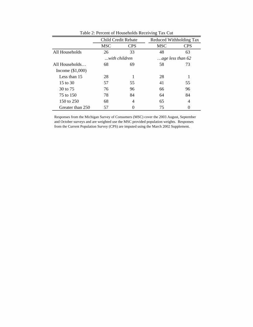
Table 2 compares the percent of households imputed to have received the child credit rebate
and a reduction in withholdings with the percent of households in the MSC that reported
receiving the tax cuts. The table shows a high degree of awareness of the advance child credit
rebate checks. Among all households, 26 percent of respondents in the MSC reported receiving
a child credit rebate check compared to 33 percent of all households imputed in the CPS. This
small difference disappears when restricting the sample to households with children. The
awareness of changes in withholding was smaller. While only 48 percent of households reported
a change in their withholdings, the imputations in the CPS suggest 63 percent of households had
a reduction in withholdings, a share similar to estimated provided by the Congressional Budget
Office. Restricting the sample to households less than age 62 does not eliminate the difference,
although both shares increase 10 percentage points.
Table 2 also reports the percent of households receiving a tax cut by income class. Among
households with children, there are some distinct differences between the percent of MSC
respondents receiving the child credit rebate and the imputed percent from the CPS by income.
In both the MSC and the CPS, households in the highest and lowest income categories were less
likely to report receiving a check. In general, the relationship between income in the MSC and
receipt of the rebate check is weaker than in the CPS. This is most true at the tails of the income
distribution where fewer households should have received an advance child credit rebate.
12 AGI is top coded at $99,999 in the CPS. For those households with AGI in excess of $99,999 we constructed an AGI equal to total family income plus capital gains less non-taxed income like workmen’s compensation, social security, and SSI benefits.

11
One potential explanation for the differences in the receipt of a rebate check by income group
between the MSC and the CPS is that households in the MSC were not aware of the income
limits for the rebate checks, and that many lower or higher income households anticipated
receiving a check when they were not entitled. However, an examination of the differences in
responses across the August, September, and October surveys does not show the systematic
pattern one might expect in this case—that is, perceived eligibility for the rebate checks did not
decline over time. Instead, a more likely explanation is that the household income response in
the MSC is a less accurate measure of taxable income than in the CPS, where efforts are made to
make sure income measures are accurate. In addition, measurement error is amplified by the
smaller cell sizes for the high and low income groups.
As with the child credit, Table 2 also shows a weaker relationship in the MSC between
income and a reduction in withholding taxes than indicated in the CPS. The differences are
smallest in the largest income groups and largest in the tails of the income distribution, an
indication again of potential measurement error. Still, relative to the CPS, there is a 30
percentage point underreporting in the MSC among households with income between $30,000
and $75,000. While almost all households in the CPS in this income class are imputed to have
received a reduction in withholding taxes, only 66 percent of the households in the MSC report
receiving a reduction.
The comparison of the MSC results and the CPS imputations suggests that the bulk of the
population appear to have been aware of receiving the boost to disposable income from the tax
cut. Households were quite aware of the rebate checks and were also aware, but less so, of the
withholding changes. To the degree that this comparison indicates errors in awareness, they are
concentrated in the tails of the income distribution. The fairly high degree of awareness suggests
that the examination of self-reported responses to the tax cut is certainly worth pursuing.
Survey Results
The spending response of households that reported receiving the child credit rebate are
shown in Table 3 and the responses for households that reported receiving an increase in take
home pay are shown in Table 4. Overall, 27.0 percent of those who reported receiving the child
credit rebate said they saved most of it, 49.0 percent said they mostly paid down debt, and 24.0
percent reported they mostly spent the rebate. Among those who said they had received an

12
increase in take home pay, 36.8 percent reported saving most of it, 42.5 percent said they mostly
paid off debt, and 20.7 percent said they spent most of the increase in pay.
If the tax cuts were viewed as permanent, we would expect forward-looking households to
spend most of the increase in disposable income. However, as indicated in Table 1, the
JGTRRA was not a permanent tax cut. Indeed, the marginal increase in future disposable
income owing to the JGTRRA was smaller than the increase due to the EGTRRA. As a result,
the spending response to the JGTRRA should be smaller than the response to the EGTRRA.
However, the fraction of households spending most of either the child credit or the reduced
withholdings was actually a bit larger than the 21.8 percent of households that reported spending
most of the EGTRRA, as reported in Shapiro and Slemrod (2003a).
Tables 3 and 4 present the spending responses by various categories of observable
characteristics. In general, the percent of households that reported spending most of the proceeds
of their tax cuts rises with income, stock ownership, education, and age. These results are
consistent with the findings in Shapiro and Slemrod (2003) and at first blush might appear to
contradict the notion that people with low-income and low-education are more likely to face
liquidity constraints or follow rule of thumb behavior and thus consume a larger share of income
changes. However, these patterns are reversed if we assume households that reported using the
tax cut to pay down debt actually boosted spending quickly after paying down their debt. There
is some evidence for this behavior in response to the 2001 EGTRRA. Agarwal, Liu and Souleles
(2004) show that households who used their tax cut to pay down credit card debt did so only
temporarily and that after a one-year period credit card debt was back to the pre-tax cut level,
indicating that the tax cut was spent. Focusing only on the percentage of households that
reported saving the child credit rebate in Table 3, there is a strong positive relationship between
income and the share of households that report saving most of the rebate. As indicated in Table
4, the relationship is weaker for the reduction in withholdings but still positive.
We examine the share of households that reported that they will spend most of the tax cut
within a year in order to see if households that paid off debt were expecting to increase their
spending in the near future. These results are reported in the final columns of Table 3 and 4 and
do not support the hypothesis that most of the households that pay off debt will quickly increase
spending. This is consistent with the results in Shapiro and Slemrod (2003b) who use the small
13
panel component of the MSC to show that households did not change their spending response
roughly six months later.
Differences between checks and withholding
As noted above, one difference between a tax cut delivered through a one-time payment—
such as the mail-out rebate of the 2003 increase in the child credit—and a tax cut spread out over
time—such as the provisions of the JGTRRA that reduced withholdings—is that people may be
more likely to notice a one-time payment opposed to a more gradual reduction in withholdings.
In this section, we examine the differences in spending responses for those who report receiving
both the rebate check and the reduction in withholding. In particular, we examine whether
households were more likely to report spending most of their rebate checks than they were their
reduced withholding.
The MCS sample contains 306 households that reported receiving both a child credit rebate
check and reduced withholdings. Table 5 shows the spending responses of these households.
Overall, households seem to have made little distinction between the rebate checks and their
reduced withholdings—with roughly two-thirds planning to use the child credit rebate check and
the increase in take-home pay in an identical manner (spend, save, or pay down debt). Even over
the course of a year there is little difference in the spending plans for the child credit rebate and
the reduction in withholdings. As indicated in Tables 3 and 4, the share of households planning
on spending most of their tax cut increases by about 5 to 10 percentage points when the time
horizon is expanded from the second half of 2003 to a year. Table 5 shows that the same is true
for households that received both the increased child credit and the reduced withholdings, with
the percent of households expecting to spend most of the income from both tax cut provisions
increasing from 11.6 percent over 2003H2 to 17.8 percent over the subsequent year.
The reduction in withholdings is a tax cut that increases the take-home pay of every
paycheck between 2003 and 2005, while the child credit rebate check is a one-time payment,
paid out in third quarter of 2003.13 Households that prefer to smooth their consumption should
have saved most of the child credit rebate and spread it over the year and spent a larger share of
the reduced withholdings because it was already smoothed. The results in Tables 3, 4 and 5 are
13 As noted above, the JGTRRA also includes an increase in the 2004 child credit but this was not referenced in the survey question.
14
somewhat surprising because the spending response to the child rebate is roughly as large as the
spending response to the reduction in withholdings, implying that the highly visible form in
which the child credit rebate was paid out had an effect. However, most analysts at the time
expected the child credit rebate to provide an immediate boost to spending that would be greater
than the stimulus from the reduced withholdings. Based on the MSC data, this does not appear
to have happened.
Unfortunately, it is difficult to make any strong conclusions about consumption smoothing
behavior because we do not know the types of expenditures that were financed with the tax cut.
For example, the consumption induced by the rebate check may have been smoothed the same as
the consumption induced by the reduction in withholdings if households were more likely to
spend the rebate check on a durable good, such as a car or television (Mankiw, 1982).14 To
determine if the type of consumption goods financed by the child credit rebate differed
substantially from those financed by the reduced withholdings, we examined the buying attitudes
provided in the MSC.
As indicated in Table 6, 72.2 percent of all households claimed it was a “good time” to buy a
car, and 68.5 percent claimed it was a “good time” to buy a major household appliance such as
furniture, a refrigerator, a stove, or a television. Receiving either the child credit rebate or a
reduction in withholdings (or both) does not seem to have changed people’s feelings about
buying a car or major appliance. However, not surprisingly, households that reported spending
most of their child credit rebate felt on average that it was a better time to buy a car than did all
households on average. Households that reported spending most of their reduced withholdings
felt it was a better time than the average household to purchase both cars as well as other major
appliances.
Comparing the buying attitudes of households that spent most of their child credit rebate to
those that spent most of their reduced withholdings provides little support for the hypothesis that
the child credit rebate was more likely to be used to purchase a durable good. Indeed, the
opposite hypothesis cannot be rejected. While 76.8 percent of households that spent most of
their child credit rebate felt it was a good time to buy a car and 65.9 percent felt it was a good
time to buy a major appliance, 82.2 percent of households that spent most of their reduced
14 Many retailers ran advertisements in the summer of 2003 encouraging households to spend their rebate checks. Indeed, retailers such as Home Depot, Sears and Wal-Mart advised consumers to cash their rebate check at the store while making a purchase. Big-ticket durable items were highly promoted during this advertising blitz.

15
withholdings claimed it was a good time to buy a car and 77.9 percent were optimistic about
purchasing a major appliance. Neither of these differences can be rejected at a 10 percent level
of significance.
The bottom two rows of Table 6 control for differences across households receiving the child
credit rebate, which favored lower to middle income households, and households that received
reduced withholdings, which favored middle to upper income households. On average,
households that only received a reduction in withholdings had about $30,000 more income than
households that only received a child credit rebate. Restricting the sample to households that
received both tax cut provisions, 82.5 percent of those that spent most of their child rebate felt it
was a good time to buy a car and 62.5 percent felt it was a good time to buy a major appliance.
By comparison, a smaller 73.8 percent of those that spent most of their reduced withholdings
were optimistic about purchasing a car while a larger 75.3 percent were upbeat about buying a
major appliance. Both of these differences are rejected at a 10 percent level of significance,
suggesting the child credit rebates were no more likely than the reduced withholdings to have
been smoothed in terms of consumption by way of the purchase of durable goods.
Estimating the Marginal Propensity to Consume
The advantage of the MSC data compared to data on consumer expenditures is that it relates
to the change in household spending given the tax cuts compared to what households believed
their spending would have been in the absence of the tax cuts. Consequently, the marginal
propensity to consume can be examined in a way that cannot be done with expenditure data.
More formally, we consider a model of the household spending response iS to the tax cut iτ that
allows for both observed and unobserved heterogeneity in the MPC:
( )i i i iS Xμ γ η τ′= + , (1)
where (.)μ is an approximation to household i’s MPC out of the tax cut with 0 ( ) 1zμ< < and
( ) 0z zμ∂ ∂ > for all z . The MPC varies across households by an observable vector of
household characteristics, iX , and an unobservable scaler iη , which is known to the household
and is independently and identically distributed across households with mean zero.15
15 Because the purpose of this paper is not to estimate underlying parameters of the household consumption function, this MPC is general enough that it can be motivated by almost any model of consumer behavior.

16
If the MSC measured each household’s spending response, the MPC would simply be given
by the ratio of this response to an estimate of their tax cut, and the aggregate MPC would
immediately follow. Unfortunately, the spending response is unobserved. Rather, the survey
instrument measures only whether the tax cut led households to “mostly increase spending,”,
“mostly increase saving,” or to “mostly pay off debt.” That is, iS can be thought of as a latent
variable.
Let 1iI = if a household claims to have mostly increased their spending in response to the
tax cut, implying i iS λτ> for some λ to be determined, and 0iI = otherwise. The empirical
model then follows from the definition of the indicator variable and (1):
( ) ( )( )( )
( )( )1
Pr 1 , , Pr
Pr
Pr ,
i i i i i
i i
i i
I X S
X
X
τ λ λτ
μ γ η λ
η γ μ λ−
= = >
= + >
= < −
(2)
where the last equality follows from the assumption that (.)μ is monotonically increasing and iη
is symmetric around zero.
The marginal propensity to consume can be identified by maximum likelihood using (2),
given the distribution of η , a function (.)μ , and a value for λ . We assume ~ (0,1)Nη and
(.)μ is a cumulative standard normal function. The value for λ is related to the survey
question. Typically, the term “mostly” would refer to one-half and so 1/ 2λ = . However, the
respondents were given three choices in the survey: mostly increase spending, mostly increase
saving, or mostly pay off debt. As a result, some households could have “mostly spent” the tax
cut while still spending less than one-half of it. The smallest share of the tax cut a household
could spend while still spending a plurality is one-third, suggesting 1/ 3 1/ 2λ≤ ≤ . We split this
difference and set 5 /12λ = , although our results for the effect of the tax cut on aggregate
personal consumption expenditures are not greatly affected by setting λ equal to 1/3 or 1/2.
Table 7 reports the results from estimating (2) under the above assumptions controlling for
demographic and financial characteristics. Consistent with the life-cycle hypothesis, households
headed by older individuals appear to have consumed a larger share of both the child credit
rebate and the reduction in withholdings, both contemporaneously (2003H2) and over the
subsequent year (through 2004H1). In contrast to the univariate relationship noted in Tables 3
17
and 4, there is no significant relationship between asset ownership and the spending response out
of the child credit rebate after controlling for age and income. With regard to the reduced
withholdings, although stock ownership boosted the spending response by one-third on average,
all else equal, this is more than offset by home ownership, which appears to have reduced the
spending response out of the reduction in withholdings by almost one-half on average.16
Consequently, there is little support for the hypothesis that liquidity constraints boosted the
MPC’s of low wealth households.
The relationship between income and the contemporaneous MPC out of both tax cuts is
insignificant for incomes below $75,000. However, households with income between $75,000
and $100,000 have an MPC out of the reduction in withholdings that is 23 percent larger than
households with income less than $30,000. Households with income greater than $100,000 have
an MPC out the reduction in withholdings that is 38 percent larger. This positive relationship is
at odds with the conventional wisdom that households with higher income tend to have a higher
propensity to save (Dynan, Skinner and Zeldes, 2004). Even after controlling for education as a
proxy for permanent income, the estimated relationship between income and the MPC is
positive.17 The MSC also asks households about whether they expect their earnings growth to
keep pace with the rate of inflation. Not surprisingly, households that were more optimistic
about their future real income growth spent roughly one-third more of both their tax cuts than the
average household. In general, the relationship between the MPC and income does not change
when the spending response is extended to the entire year following the tax cut.
We next examine the distribution of the estimated MPC across households. Without
observing η , we can only consider the expected value of a household’s MPC, which we estimate
numerically.18 The last two rows of Table 7 report the mean and standard deviation of the
expected MPC out of the child credit rebate and the reduced withholdings. There is little
difference between the mean MPC out of the child credit rebate and the mean MPC out of the
reduction in withholdings. In both cases, the average household expected to spend or had spent
roughly one-quarter of both tax cuts in the second half of 2003. In the year following the tax cut, 16 All marginal effects are computed by taking the difference between the imputed MPC with the dummy variable in question set to 1 less the imputed MPC with the dummy variable set to 0. All other variables are set to the sample median, and the unobserved component η is set to zero. 17 These results are not shown in the Table 7. 18 We estimate [ ( )]i iE Xμ γ η′ + for each household by simulating ( )i iXμ γ η′ + with 1,000 draws from a standard normal and taking its mean.

18
the average household expected to spend roughly one-third of the child credit rebate and the
reduced withholdings. However, the step-up in spending out of the reduced withholdings was
somewhat larger than the step-up in spending out of the child credit rebate, consistent with the
reduced withholdings affecting permanent income more so than the one-time rebate check.
The average MPC’s in Table 7 are similar to the share of households reporting to have
mostly increased their spending in response to the tax cuts, as indicated in Tables 3 and 4.
However, because the estimated MPC’s are partly determined by the identifying assumptions for
the distribution of η , the function (.)μ , and the value for λ , the similarity in the results was by
no means inevitable. Indeed, a distribution of η with less mass in its tails, or a function (.)μ
and value λ that generates a larger value for 1( )μ λ− would yield a larger estimated MPC. To
the extent that the identifying assumptions are plausible, the results in Table 7 provide a
reasonable estimate of each household’s MPC out of the tax cut. In contrast, the share of
households reporting to have spent “most” of the tax cut cannot be interpreted as an MPC either
for an individual household or for the aggregate.
Aggregate Spending Response
In terms of dollar value, the child credit increase favored middle income households while
the reduced withholdings largely favored higher income households. In addition, the results in
Table 7 suggest households with more income spent a larger share of their tax cut.
Consequently, the aggregate spending response cannot be obtained by simply applying the mean
MPC reported in Table 7 to the aggregate tax cut. To compute the aggregate spending response,
we first estimate the mean of the MPC’s by income class using the empirical model described
above.19 We then compute the share of the aggregate tax cut by income class using an imputed
tax cut from the March supplement of the 2002 CPS. The spending response within each income
class is then computed as the product of the MPC and tax cut. The aggregate spending response
is the sum across income classes and the aggregate MPC is defined as the ratio of the aggregate
spending response to the aggregate tax cut. These results are reported in Table 8.
The child credit rebate boosted total real spending by an estimated $4 billion dollars in the
second half of 2003. The spending response was largest among households earning between
19 These estimates are interpreted only as descriptive of the spending response within income groups.

19
$30,000 and $75,000 per year. This reflects the fact these households received the largest share
of the child credit rebate and not that they had a higher MPC, which was smaller than that of
households with higher income. Not surprisingly, the aggregate spending response to the one-
time child credit rebate did not increase much beyond 2003, only increasing $0.7 billion in the
first half of 2004 as indicated by the difference between the bottom and top panels of Table 8.
The reduced withholdings boosted total real spending by about $6 billion in the second half
of 2003, as indicated in Table 8. Unlike the response to the child credit rebate, the spending
response to the reduced withholdings is largely concentrated among households with annual
income greater than $100,000, reflecting both a larger estimated MPC and the fact that these
households received 2/3 of the withholdings reduction. The spending response to the reduced
withholdings rose to about $14 billion in the first half of 2004 and was again, largely
concentrated among high income households. This skewed distribution of the tax cut across
income groups yields an aggregate MPC that is about 20 percent larger than the mean of the
MPC’s across all households.
The last three columns of Table 8 combine the responses to the child credit rebate and the
reduced withholdings. Total real spending was boosted by $10 billion in the second half of 2003
implying an aggregate MPC of 0.28, and by $15 billion in the first half of 2004 implying a
cumulative aggregate MPC of 0.36. In general, the spending response was concentrated among
higher income households with about one-half of the total increase in spending attributed to
households earning more than $100,000.
Conclusion
Using household survey data on the self-reported qualitative response to the tax cuts enacted
as part of the Jobs and Growth Tax Relief and Reconciliation Act of 2003, we estimate that the
aggregate personal consumption expenditures was boosted in the second half of 2003 by
$9.7 billion from the child credit rebate and the reduction in withholdings. Depending on how
households interpreted the survey question, the actual boost to personal consumption
expenditures may have been larger than we estimate. In particular, the survey does not ask about
the response to the AMT and dividend tax relief, which combine to make up roughly one-half of
the total value of the tax cut. Nor does our estimate include any potential feedback effect from
the initial increase in output. Indeed, this could partially explain why the estimated spending
20
response is roughly 1/3 as large as the actual step-up in aggregate real personal consumption
expenditures over that time period. In contrast, the estimated spending response is about two
times larger than the response implied by the permanent income hypothesis. This discrepancy
does not appear to be a result of liquidity constraints: We find no relationship between the
contemporaneous MPC out of the tax cuts and household asset holdings and a positive
relationship with income.
We estimate the JGTRRA boosted aggregate personal consumption expenditures by
$15 billion in the first half of 2004. This is in contrast to a step-down in the growth of actual
aggregate personal consumption expenditures in 2004H1. However, it is difficult to disentangle
the continuing effects of the JGTRRA in early 2004 from the effects of the near-record jump in
oil prices that occurred at that time.
Contrary to conventional wisdom, there is little evidence that households spent a larger share
of their child credit rebate than of their reduced withholdings. However, this result is also
inconsistent with economic theory, which suggests households should have spent a smaller share
of the child credit rebate. The marginal propensity to consume was about the same for both tax
cuts and equal to roughly 1/4. We also find no evidence indicating that the rebate check was
more likely to be spent on durable goods.

21
References
Agarwal, Sumit, Liu, Chunlin, and Souleles, Nicholas S. “The Response of Consumer Spending and Debt to Tax Rebates -- Evidence from Consumer Credit Data.” The Wharton School working paper, 2004.
Barro, Robert J. "Are Government Bonds Net Wealth." Journal of Political Economy, 1974, 82 (6), 1095-1117.
Bertrand, Marianne, Mullainathan, Sendhil. "Do People Mean What They Say? Implications for Subjective Survey Data." American Economic Review, 2001, 91 (2), 67-72.
Browning, Martin, Lusardi, Annamaria. "Household Saving: Micro Theories and Micro Facts." Journal of Economic Literature, 1996, 34 1797-1855.
Campbell, John Y., Mankiw, N. Gregory. "Consumption, Income, and Interest Rates: Reinterpreting the Time Series Evidence," Blanchard, Olivier J., Fischer, Stanely, NBER Macroeconomics Annual 1989. Cambridge, MA: MIT Press, 1989, 185-216.
Dynan, Karen E., Skinner, Jonathan, Zeldes, Stephen P. "Do the Rich Save More?" Journal of Political Economy, 2004, 112 (2), 397-444.
Johnson, David S., Parker, Jonathan A., Souleles, Nicholas S. "The Response of Consumer Spending to the Randomized Income Tax Rebates of 2001." The Wharton School working paper, February 2004.
Michel, Norbert J. and Rector, Ralph A. “Was the 2001 Tax Rebate Effective Stimulus Policy? Using the Consumer Expenditure Survey to Test Whether Consumers Spent Their Rebate Checks.” Heritage Foundation working paper, June 2004.
Mankiw, N. Gregory. Press briefing, Washington, D.C., Council of Economic Advisers, February 9, 2004.
_______. “Hall's Consumption Hypothesis and Durable Goods.” Journal of Monetary Economics, 1982, 10, 181-196.
Modigliani, Franco and Steindel, Charles. "Is a Tax Rebate an Effective Tool for Stabilization Policy?" Brookings Papers on Economic Activity, 1977, 1977 (1), 175-209.
Parker, Jonathan A. "The Reaction of Household Consumption to Predictable Changes in Payroll Tax Rates." American Economic Review, 1999, 89 (4), 413-418.
Poterba, James M. "Are Consumers Forward Looking? Evidence from Fiscal Experiments." American Economic Review, 1988, 78 (2), 413-418.
Shapiro, Matthew D., Slemrod, Joel. "Consumer Response to Tax Rebates." American Economic Review, 2003, 93 (1), 381-396.
_______. "Consumer Response to the Timing of Income: Evidence from a Change in Tax Withholding." American Economic Review, 1995, 85 (1), 274-283.
_______. "Did the 2001 Tax Rebate Stimulate Spending? Evidence from Taxpayer Surveys," Poterba, James, Tax Policy and the Economy. Cambridge: MIT Press, 2003.
Souleles, Nicholas S. "Consumer Response to the Reagan Tax Cuts." Journal of Public Economics, 2002, 85, 99-120.
_______. "The Response of Household Consumption to Income Tax Refunds." American Economic Review, 1999, 89 (4), 947-958.
Tax Policy Center. “Conference Agreement on the Jobs and Growth Tax Relief Reconciliation Act of 2003: Distribution of Income Tax Change by AGI Class, 2003.” Table T03-0107, May 22, 2003.
Wilcox, David W. Social Security Benefits. “Consumption Expenditures, and the Life-Cycle Hypothesis.” Journal of Political Economy, 1989, 97(2), 288-304.
Wilcox, David W. "Income Tax Refunds and the Timing of Consumption Expenditure." Federal Reserve Board Working Paper, 1990.

2003H2 2004 2005 2006-2010 PDVTotal 35 101 58 91 275
(37) (110) (65) (107)...Increased Child Credit 15 5 11 0 30
(16) (5) (12) (0)...Lowered Withholdings 20 66 21 0 106
(21) (72) (24) (0)...AMT & Dividend Tax Relief 0 30 26 91 139
(0) (33) (29) (107)
Table 1: Effect of the JGTRRA on Real Disposable Income (Billions of 2000 $)
The estimated magnitude of the tax cut comes from the Joint Committee on Taxation at the time the JGTRRA was enacted. Real values are computed using the forecasted CPI-U from the February, 2003 Economic Report of the President (ERP), converted to 2000 dollars. Nominal values are in parentheses. The 2006-2010 column reports the sum of the tax cut over those years. The final column reports the real present discounted value of the tax cut as of 2003Q3 using the projected rate of the 3-month Treasury bill from the February, 2003 ERP less the projected percent change in the CPI-U (beyond 2005, the real interest is set to 2 percent).
MSC CPS MSC CPSAll Households 26 33 48 63
All Households… 68 69 58 73Income ($1,000)
Less than 15 28 1 28 115 to 30 57 55 41 5530 to 75 76 96 66 9675 to 150 78 84 64 84150 to 250 68 4 65 4Greater than 250 57 0 75 0
Table 2: Percent of Households Receiving Tax CutChild Credit Rebate Reduced Withholding Tax
...with children …age less than 62
Responses from the Michigan Survey of Consumers (MSC) cover the 2003 August, September and October surveys and are weighted use the MSC provided population weights. Responses from the Current Population Survey (CPS) are imputed using the March 2002 Supplement.

All Eligible Households 386 100.0 27.0 49.0 24.0 30.1Income ($1,000)
Less than 30 80 24.4 17.6 62.6 19.8 25.530 to 75 165 44.6 25.5 53.1 21.4 29.4750 to 100 71 17.8 34.7 34.0 31.3 36.4Greater than 100 51 13.2 45.6 17.5 36.8 36.8
Corporate EquitiesDon't own 132 35.8 23.2 57.6 19.2 25.3Own 254 64.2 29.2 44.2 26.6 32.8
Education of HeadNo high school degree 24 6.7 28.6 62.9 8.6 19.0High school degree 105 29.1 23.8 52.3 23.8 33.3Some College 91 23.3 23.7 53.7 22.6 30.3College degree 166 40.8 31.0 41.7 27.4 29.6
Age of HeadLess than 45 301 81.0 27.8 50.3 22.0 27.945 to 62 80 17.5 26.1 41.9 32.0 39.7Greater than 62 4 1.4 0.0 57.1 42.9 42.9
Table 3: Responses to the Child Credit Rebate
N Percent Eligible Spend
Response (percent)
Save Reduce Debt
Spend within a Year
Responses from the Michigan Survey of Consumers (MSC) cover the 2003 August, September and October surveys and are weighted use the MSC provided population weights. Cell counts did not sum to total due to missing values.

All Eligible Households 730 100.0 36.8 42.5 20.7 32.4Income ($1,000)
Less than 30 129 21.3 30.7 53.7 15.5 25.030 to 75 333 47.1 36.4 43.9 19.7 32.3750 to 100 107 15.0 42.4 33.6 24.1 35.8Greater than 100 116 16.6 34.2 30.2 35.6 51.7
Corporate EquitiesDon't own 224 32.1 32.9 51.7 15.3 27.4Own 506 67.9 38.7 38.2 23.2 34.7
Education of HeadNo high school degree 25 3.5 27.5 54.9 17.6 27.4High school degree 171 24.5 35.0 47.7 17.2 30.7Some College 174 24.3 33.5 45.2 21.3 36.8College degree 360 47.7 40.1 37.5 22.4 31.4
Age of HeadLess than 45 433 63.8 37.7 44.0 18.4 32.545 to 62 248 29.1 33.5 44.3 22.3 30.2Greater than 62 45 6.7 43.0 22.3 34.7 40.4
N Percent Eligible Spend
Table 4: Responses to the Reduced Withholding TaxResponse (percent)
Save Reduce Debt
Spend within a Year
Responses from the Michigan Survey of Consumers (MSC) cover the 2003 August, September and October surveys and are weighted use the MSC provided population weights. Cell counts did not sum to total due to missing values.

Child Credit RebateSave Reduce
debt Spend Total Spend within a year
Save 22.0 5.0 3.8 30.8 8.3Reduce debt 10.6 31.9 5.2 47.8 11.9Spend 4.5 5.3 11.6 21.4 12.7Total 37.1 42.3 20.6 100.0 32.9Spend within a year 5.8 8.1 13.9 27.9 17.8
Reduced Withholding TaxTable 5: Percent Response Among Households Receiving Both Tax Cuts
Responses from the Michigan Survey of Consumers (MSC) cover the 2003 August, September and October surveys and are weighted use the MSC provided population weights.

Percent p- value Percent p- valueAll Households 72.2 68.5 Received… Child Credit Rebate 73.8 66.4 Reduced Withholding Tax 74.2 68.6 Received and spent most of… Child Credit Rebate 76.8 65.9 Reduced Withholding Tax 82.0 77.9 Received both and spent most of… Child Credit Rebate 82.5 62.5 Reduced Withholding Tax 73.8 75.3
0.04
0.17 0.86
0.06
Table 6: Households Claiming "Good Time" to BuyCar Major Appliance
0.32 0.63

Spend within a year
Spend within a year
Constant -0.88 -0.90 -0.61 -1.16 -1.19 -0.88(0.23) (0.23) (0.22) (0.17) (0.17) (0.16)
Age: 44 or younger -0.36 -0.39 -0.43 -0.14 -0.19 0.06(0.18) (0.19) (0.18) (0.12) (0.13) (0.12)
Age: 62 or older 0.31 0.33 0.17 0.58 0.58 0.49(0.58) (0.58) (0.58) (0.23) (0.23) (0.22)
Own Home 0.02 0.04 -0.09 -0.29 -0.28 -0.38(0.19) (0.20) (0.18) (0.15) (0.15) (0.13)
Own Stocks 0.17 0.13 0.14 0.24 0.21 0.13(0.17) (0.18) (0.17) (0.14) (0.14) (0.12)
Income: $30,000 to $75,000 0.06 0.04 0.14 0.19 0.19 0.29(0.21) (0.21) (0.20) (0.17) (0.17) (0.15)
Income: $75,000 to $100,000 0.29 0.27 0.27 0.35 0.33 0.41(0.25) (0.25) (0.24) (0.21) (0.21) (0.19)
Income: greater than $100,000 0.29 0.20 0.14 0.49 0.41 0.57(0.27) (0.28) (0.27) (0.21) (0.21) (0.19)
Expected Real Income Growth 0.24 0.28 0.25 0.13(0.17) (0.16) (0.13) (0.12)
Log-Likelihood -202.2 -201.2 -224.6 -338.3 -336.4 -421.6Marginal Propensity to Consume
Mean 0.26 0.26 0.30 0.23 0.23 0.33Standard Deviation 0.05 0.06 0.06 0.06 0.06 0.07
Child Credit Rebate Reduced Withholding TaxTable 7: Estimating the Marginal Propensity to Consume
Spend now Spend now
Standard errors are in parentheses.

Tax Cut MPC Spending Tax Cut MPC Spending Tax Cut MPC Spending
All Households 15.1 0.27 4.0 20.1 0.28 5.7 35.2 0.28 9.7Income ($1,000)
Less than 30 1.6 0.23 0.4 0.1 0.20 0.0 1.7 0.23 0.430 to 75 8.7 0.24 2.1 3.1 0.22 0.7 11.9 0.23 2.875 to 100 3.0 0.33 1.0 3.0 0.28 0.8 6.0 0.30 1.8Greater than 100 1.8 0.32 0.6 13.8 0.30 4.1 15.6 0.30 4.7
All Households 15.1 0.31 4.7 53.5 0.38 20.1 68.7 0.36 24.8Income ($1,000)
Less than 30 1.6 0.27 0.4 0.4 0.27 0.1 2.0 0.27 0.530 to 75 8.7 0.29 2.6 8.3 0.31 2.6 17.1 0.30 5.175 to 100 3.0 0.37 1.1 7.9 0.37 2.9 10.9 0.37 4.1Greater than 100 1.8 0.35 0.6 36.9 0.39 14.5 38.7 0.39 15.1
2003H2
2003H2 & 2004H1
Table 8: JGTRRA and the Aggregate Spending ResponseChild Credit Rebate Reduced Withholding Total
Dollar values are in billions of 2000 dollars, deflated using the implicit price deflator for total personal consumption expenditures in the NIPA. Estimates of the tax cut for all households come from the Joint Committee on Taxation, which is then decomposed by income group using the estimated shares of the tax cut imputed using the CPS March 2002 supplement. The total tax cut is the sum of the child credit rebate and reduced withholdings; it does not include the AMT, dividend tax, and marriage penalty relief. MPC's are estimated over the MSC data using the methodology described in the text. Aggregate MPC's (either for all households or for the total tax cut) are defined as the ratio of the aggregate spending response to the aggregate tax cut.