the - iaria journals · juan j. flores, universidad michoacana, mexico ... mohamed graiet, institut...
TRANSCRIPT


The International Journal on Advances in Networks and Services is published by IARIA.
ISSN: 1942-2644
journals site: http://www.iariajournals.org
contact: [email protected]
Responsibility for the contents rests upon the authors and not upon IARIA, nor on IARIA volunteers,
staff, or contractors.
IARIA is the owner of the publication and of editorial aspects. IARIA reserves the right to update the
content for quality improvements.
Abstracting is permitted with credit to the source. Libraries are permitted to photocopy or print,
providing the reference is mentioned and that the resulting material is made available at no cost.
Reference should mention:
International Journal on Advances in Networks and Services, issn 1942-2644
vol. 10, no. 1 & 2, year 2017, http://www.iariajournals.org/networks_and_services/
The copyright for each included paper belongs to the authors. Republishing of same material, by authors
or persons or organizations, is not allowed. Reprint rights can be granted by IARIA or by the authors, and
must include proper reference.
Reference to an article in the journal is as follows:
<Author list>, “<Article title>”
International Journal on Advances in Networks and Services, issn 1942-2644
vol. 10, no. 1 & 2, year 2017, <start page>:<end page> , http://www.iariajournals.org/networks_and_services/
IARIA journals are made available for free, proving the appropriate references are made when their
content is used.
Sponsored by IARIA
www.iaria.org
Copyright © 2017 IARIA

International Journal on Advances in Networks and Services
Volume 10, Number 1 & 2, 2017
Editor-in-Chief
Tibor Gyires, Illinois State University, USA
Editorial Advisory Board
Mario Freire, University of Beira Interior, PortugalCarlos Becker Westphall, Federal University of Santa Catarina, BrazilRainer Falk, Siemens AG - Corporate Technology, GermanyCristian Anghel, University Politehnica of Bucharest, RomaniaRui L. Aguiar, Universidade de Aveiro, PortugalJemal Abawajy, Deakin University, AustraliaZoubir Mammeri, IRIT - Paul Sabatier University - Toulouse, France
Editorial Board
Ryma Abassi, Higher Institute of Communication Studies of Tunis (Iset'Com) / Digital Security Unit, TunisiaMajid Bayani Abbasy, Universidad Nacional de Costa Rica, Costa RicaJemal Abawajy, Deakin University, AustraliaJavier M. Aguiar Pérez, Universidad de Valladolid, SpainRui L. Aguiar, Universidade de Aveiro, PortugalAli H. Al-Bayati, De Montfort Uni. (DMU), UKGiuseppe Amato, Consiglio Nazionale delle Ricerche, Istituto di Scienza e Tecnologie dell'Informazione (CNR-ISTI),ItalyMario Anzures-García, Benemérita Universidad Autónoma de Puebla, MéxicoPedro Andrés Aranda Gutiérrez, Telefónica I+D - Madrid, SpainCristian Anghel, University Politehnica of Bucharest, RomaniaMiguel Ardid, Universitat Politècnica de València, SpainValentina Baljak, National Institute of Informatics & University of Tokyo, JapanAlvaro Barradas, University of Algarve, PortugalMostafa Bassiouni, University of Central Florida, USAMichael Bauer, The University of Western Ontario, CanadaCarlos Becker Westphall, Federal University of Santa Catarina, BrazilZdenek Becvar, Czech Technical University in Prague, Czech RepublicFrancisco J. Bellido Outeiriño, University of Cordoba, SpainDjamel Benferhat, University Of South Brittany, FranceJalel Ben-Othman, Université de Paris 13, FranceMathilde Benveniste, En-aerion, USALuis Bernardo, Universidade Nova of Lisboa, PortugalAlex Bikfalvi, Universidad Carlos III de Madrid, SpainThomas Michael Bohnert, Zurich University of Applied Sciences, SwitzerlandEugen Borgoci, University "Politehnica"of Bucharest (UPB), RomaniaFernando Boronat Seguí, Universidad Politecnica de Valencia, SpainChristos Bouras, University of Patras, GreeceMahmoud Brahimi, University of Msila, AlgeriaMarco Bruti, Telecom Italia Sparkle S.p.A., ItalyDumitru Burdescu, University of Craiova, Romania

Diletta Romana Cacciagrano, University of Camerino, ItalyMaria-Dolores Cano, Universidad Politécnica de Cartagena, SpainJuan-Vicente Capella-Hernández, Universitat Politècnica de València, SpainEduardo Cerqueira, Federal University of Para, BrazilBruno Chatras, Orange Labs, FranceMarc Cheboldaeff, T-Systems International GmbH, GermanyKong Cheng, Vencore Labs, USADickson Chiu, Dickson Computer Systems, Hong KongAndrzej Chydzinski, Silesian University of Technology, PolandHugo Coll Ferri, Polytechnic University of Valencia, SpainNoelia Correia, University of the Algarve, PortugalNoël Crespi, Institut Telecom, Telecom SudParis, FrancePaulo da Fonseca Pinto, Universidade Nova de Lisboa, PortugalOrhan Dagdeviren, International Computer Institute/Ege University, TurkeyPhilip Davies, Bournemouth and Poole College / Bournemouth University, UKCarlton Davis, École Polytechnique de Montréal, CanadaClaudio de Castro Monteiro, Federal Institute of Education, Science and Technology of Tocantins, BrazilJoão Henrique de Souza Pereira, University of São Paulo, BrazilJavier Del Ser, Tecnalia Research & Innovation, SpainBehnam Dezfouli, Universiti Teknologi Malaysia (UTM), MalaysiaDaniela Dragomirescu, LAAS-CNRS, University of Toulouse, FranceJean-Michel Dricot, Université Libre de Bruxelles, BelgiumWan Du, Nanyang Technological University (NTU), SingaporeMatthias Ehmann, Universität Bayreuth, GermanyWael M El-Medany, University Of Bahrain, BahrainImad H. Elhajj, American University of Beirut, LebanonGledson Elias, Federal University of Paraíba, BrazilJoshua Ellul, University of Malta, MaltaRainer Falk, Siemens AG - Corporate Technology, GermanyKároly Farkas, Budapest University of Technology and Economics, HungaryHuei-Wen Ferng, National Taiwan University of Science and Technology - Taipei, TaiwanGianluigi Ferrari, University of Parma, ItalyMário F. S. Ferreira, University of Aveiro, PortugalBruno Filipe Marques, Polytechnic Institute of Viseu, PortugalUlrich Flegel, HFT Stuttgart, GermanyJuan J. Flores, Universidad Michoacana, MexicoIngo Friese, Deutsche Telekom AG - Berlin, GermanySebastian Fudickar, University of Potsdam, GermanyStefania Galizia, Innova S.p.A., ItalyIvan Ganchev, University of Limerick, Ireland / University of Plovdiv “Paisii Hilendarski”, BulgariaMiguel Garcia, Universitat Politecnica de Valencia, SpainEmiliano Garcia-Palacios, Queens University Belfast, UKMarc Gilg, University of Haute-Alsace, FranceDebasis Giri, Haldia Institute of Technology, IndiaMarkus Goldstein, Kyushu University, JapanLuis Gomes, Universidade Nova Lisboa, PortugalAnahita Gouya, Solution Architect, FranceMohamed Graiet, Institut Supérieur d'Informatique et de Mathématique de Monastir, TunisieChristos Grecos, University of West of Scotland, UKVic Grout, Glyndwr University, UKYi Gu, Middle Tennessee State University, USAAngela Guercio, Kent State University, USAXiang Gui, Massey University, New Zealand

Mina S. Guirguis, Texas State University - San Marcos, USATibor Gyires, School of Information Technology, Illinois State University, USAKeijo Haataja, University of Eastern Finland, FinlandGerhard Hancke, Royal Holloway / University of London, UKR. Hariprakash, Arulmigu Meenakshi Amman College of Engineering, Chennai, IndiaGo Hasegawa, Osaka University, JapanEva Hladká, CESNET & Masaryk University, Czech RepublicHans-Joachim Hof, Munich University of Applied Sciences, GermanyRazib Iqbal, Amdocs, CanadaAbhaya Induruwa, Canterbury Christ Church University, UKMuhammad Ismail, University of Waterloo, CanadaVasanth Iyer, Florida International University, Miami, USAPeter Janacik, Heinz Nixdorf Institute, University of Paderborn, GermanyImad Jawhar, United Arab Emirates University, UAEAravind Kailas, University of North Carolina at Charlotte, USAMohamed Abd rabou Ahmed Kalil, Ilmenau University of Technology, GermanyKyoung-Don Kang, State University of New York at Binghamton, USASarfraz Khokhar, Cisco Systems Inc., USAVitaly Klyuev, University of Aizu, JapanJarkko Kneckt, Nokia Research Center, FinlandDan Komosny, Brno University of Technology, Czech RepublicIlker Korkmaz, Izmir University of Economics, TurkeyTomas Koutny, University of West Bohemia, Czech RepublicEvangelos Kranakis, Carleton University - Ottawa, CanadaLars Krueger, T-Systems International GmbH, GermanyKae Hsiang Kwong, MIMOS Berhad, MalaysiaKP Lam, University of Keele, UKBirger Lantow, University of Rostock, GermanyHadi Larijani, Glasgow Caledonian Univ., UKAnnett Laube-Rosenpflanzer, Bern University of Applied Sciences, SwitzerlandGyu Myoung Lee, Institut Telecom, Telecom SudParis, FranceShiguo Lian, Orange Labs Beijing, ChinaChiu-Kuo Liang, Chung Hua University, Hsinchu, TaiwanWei-Ming Lin, University of Texas at San Antonio, USADavid Lizcano, Universidad a Distancia de Madrid, SpainChengnian Long, Shanghai Jiao Tong University, ChinaJonathan Loo, Middlesex University, UKPascal Lorenz, University of Haute Alsace, FranceAlbert A. Lysko, Council for Scientific and Industrial Research (CSIR), South AfricaPavel Mach, Czech Technical University in Prague, Czech RepublicElsa María Macías López, University of Las Palmas de Gran Canaria, SpainDamien Magoni, University of Bordeaux, FranceAhmed Mahdy, Texas A&M University-Corpus Christi, USAZoubir Mammeri, IRIT - Paul Sabatier University - Toulouse, FranceGianfranco Manes, University of Florence, ItalySathiamoorthy Manoharan, University of Auckland, New ZealandMoshe Timothy Masonta, Council for Scientific and Industrial Research (CSIR), Pretoria, South AfricaHamid Menouar, QU Wireless Innovations Center - Doha, QatarGuowang Miao, KTH, The Royal Institute of Technology, SwedenMohssen Mohammed, University of Cape Town, South AfricaMiklos Molnar, University Montpellier 2, FranceLorenzo Mossucca, Istituto Superiore Mario Boella, ItalyJogesh K. Muppala, The Hong Kong University of Science and Technology, Hong Kong

Katsuhiro Naito, Mie University, JapanDeok Hee Nam, Wilberforce University, USASarmistha Neogy, Jadavpur University- Kolkata, IndiaRui Neto Marinheiro, Instituto Universitário de Lisboa (ISCTE-IUL), Instituto de Telecomunicações, PortugalDavid Newell, Bournemouth University - Bournemouth, UKNgoc Tu Nguyen, Missouri University of Science and Technology - Rolla, USAArmando Nolasco Pinto, Universidade de Aveiro / Instituto de Telecomunicações, PortugalJason R.C. Nurse, University of Oxford, UKKazuya Odagiri, Yamaguchi University, JapanMáirtín O'Droma, University of Limerick, IrelandRainer Oechsle, University of Applied Science, Trier, GermanyHenning Olesen, Aalborg University Copenhagen, DenmarkJose Oscar Fajardo, University of the Basque Country, SpainConstantin Paleologu, University Politehnica of Bucharest, RomaniaEleni Patouni, National & Kapodistrian University of Athens, GreeceHarry Perros, NC State University, USAMiodrag Potkonjak, University of California - Los Angeles, USAYusnita Rahayu, Universiti Malaysia Pahang (UMP), MalaysiaYenumula B. Reddy, Grambling State University, USAOliviero Riganelli, University of Milano Bicocca, ItalyAntonio Ruiz Martinez, University of Murcia, SpainGeorge S. Oreku, TIRDO / North West University, Tanzania/ South AfricaSattar B. Sadkhan, Chairman of IEEE IRAQ Section, IraqHusnain Saeed, National University of Sciences & Technology (NUST), PakistanAddisson Salazar, Universidad Politecnica de Valencia, SpainSébastien Salva, University of Auvergne, FranceIoakeim Samaras, Aristotle University of Thessaloniki, GreeceLuz A. Sánchez-Gálvez, Benemérita Universidad Autónoma de Puebla, MéxicoTeerapat Sanguankotchakorn, Asian Institute of Technology, ThailandJosé Santa, University Centre of Defence at the Spanish Air Force Academy, SpainRajarshi Sanyal, Belgacom International Carrier Services, BelgiumMohamad Sayed Hassan, Orange Labs, FranceThomas C. Schmidt, HAW Hamburg, GermanyHans Scholten, Pervasive Systems / University of Twente, The NetherlandsVéronique Sebastien, University of Reunion Island, FranceJean-Pierre Seifert, Technische Universität Berlin & Telekom Innovation Laboratories, GermanyDimitrios Serpanos, Univ. of Patras and ISI/RC ATHENA, GreeceRoman Y. Shtykh, Rakuten, Inc., JapanSalman Ijaz Institute of Systems and Robotics, University of Algarve, PortugalAdão Silva, University of Aveiro / Institute of Telecommunications, PortugalFlorian Skopik, AIT Austrian Institute of Technology, AustriaKarel Slavicek, Masaryk University, Czech RepublicVahid Solouk, Urmia University of Technology, IranPeter Soreanu, ORT Braude College, IsraelPedro Sousa, University of Minho, PortugalCristian Stanciu, University Politehnica of Bucharest, RomaniaVladimir Stantchev, SRH University Berlin, GermanyRadu Stoleru, Texas A&M University - College Station, USALars Strand, Nofas, NorwayStefan Strauβ, Austrian Academy of Sciences, AustriaÁlvaro Suárez Sarmiento, University of Las Palmas de Gran Canaria, SpainMasashi Sugano, School of Knowledge and Information Systems, Osaka Prefecture University, JapanYoung-Joo Suh, POSTECH (Pohang University of Science and Technology), Korea

Junzhao Sun, University of Oulu, FinlandDavid R. Surma, Indiana University South Bend, USAYongning Tang, School of Information Technology, Illinois State University, USAYoshiaki Taniguchi, Kindai University, JapanAnel Tanovic, BH Telecom d.d. Sarajevo, Bosnia and HerzegovinaRui Teng, Advanced Telecommunications Research Institute International, JapanOlivier Terzo, Istituto Superiore Mario Boella - Torino, ItalyTzu-Chieh Tsai, National Chengchi University, TaiwanSamyr Vale, Federal University of Maranhão - UFMA, BrazilDario Vieira, EFREI, FranceLukas Vojtech, Czech Technical University in Prague, Czech RepublicMichael von Riegen, University of Hamburg, GermanyYou-Chiun Wang, National Sun Yat-Sen University, TaiwanGary R. Weckman, Ohio University, USAChih-Yu Wen, National Chung Hsing University, Taichung, TaiwanMichelle Wetterwald, HeNetBot, FranceFeng Xia, Dalian University of Technology, ChinaKaiping Xue, USTC - Hefei, ChinaMark Yampolskiy, Vanderbilt University, USADongfang Yang, National Research Council, CanadaQimin Yang, Harvey Mudd College, USABeytullah Yildiz, TOBB Economics and Technology University, TurkeyAnastasiya Yurchyshyna, University of Geneva, SwitzerlandSergey Y. Yurish, IFSA, SpainJelena Zdravkovic, Stockholm University, SwedenYuanyuan Zeng, Wuhan University, ChinaWeiliang Zhao, Macquarie University, AustraliaWenbing Zhao, Cleveland State University, USAZibin Zheng, The Chinese University of Hong Kong, ChinaYongxin Zhu, Shanghai Jiao Tong University, ChinaZuqing Zhu, University of Science and Technology of China, ChinaMartin Zimmermann, University of Applied Sciences Offenburg, Germany

International Journal on Advances in Networks and Services
Volume 10, Numbers 1 & 2, 2017
CONTENTS
pages: 1 - 11Simulating Strict Priority Queueing, Weighted Round Robin, and Weighted Fair Queueing with NS-3Robert Chang, Alphabet Inc, USAVahab Pournaghshband, Advanced Network and Security Research Laboratory, USA
pages: 12 - 24Pipeline Monitoring and Spillage Prevention Using Wireless Sensors and High Density Polyethylene PipeEncasement SystemMohammed Yusuf Agetegba, Sudan University of Science and Technology, SudanPascal Lorenz, University of Haute Alsace, France
pages: 25 - 34Indoor Localization based on Principal Components and Decision Trees in IEEE 802.15.7 Visible LightCommunication NetworksDavid Sánchez-Rodríguez, University of Las Palmas de Gran Canaria, SpainItziar Alonso-González, University of Las Palmas de Gran Canaria, SpainCarlos Ley-Bosch, University of Las Palmas de Gran Canaria, SpainJavier Sánchez-Medina, University of Las Palmas de Gran Canaria, SpainMiguel Quintana-Suárez, University of Las Palmas de Gran Canaria, SpainCarlos Ramírez-Casañas, University of Las Palmas de Gran Canaria, Spain
pages: 35 - 43Misuse Capabilities of the V2V Communication to Harm the Privacy of Vehicles and DriversMarkus Ullmann, Federal Office for Information Security & University of Applied Sciences Bonn-Rhine-Sieg,GermanyThomas Strubbe, Federal Office for Information Security, GermanyChristian Wieschebrink, Federal Office for Information Security, Germany
pages: 44 - 54SafeRFID Project: A Complete Framework for the Improvement of UHF RFID System DependabilityVincent Beroulle, Grenoble INP, FranceOum-El-Kheir Aktouf, Grenoble INP, FranceDavid Hély, Grenoble INP, France

Simulating Strict Priority Queueing, Weighted Round Robin,
and Weighted Fair Queueing with NS-3
Robert Chang and Vahab Pournaghshband
Advanced Network and Security Research LaboratoryComputer Science Department
California State University, NorthridgeNorthridge, California, [email protected]
Abstract—Strict priority queueing, weighted fair queueing, andweighted round robin are amongst the most popular differen-tiated service queueing disciplines widely used in practice toensure quality of service for specific types of traffic. In thispaper, we present the design and implementation of these threemethods in Network Simulator 3 (ns-3). ns-3 is a discrete eventnetwork simulator designed to simulate the behavior of computernetworks and internet systems. Utilizing our implementations willprovide users with the opportunity to research new solutions toexisting problems that were previously not available to solvewith the existing tools. We believe the ease of configurationand use of our modules will make them attractive tools forfurther research. By comparing the behavior of our modules withexpected outcomes derived from the theoretical behavior of eachqueueing algorithm, we were able to verify the correctness ofour implementation in an extensive set of experiments. Theseimplementations can be used by the research community toinvestigate new properties and applications of differentiatedservice queueing.
Keywords–ns-3; network simulator; differentiated service; strictpriority queueing; weighted fair queueing; weighted round robin;simulation
I. INTRODUCTION
In this paper, we present three new modules for threescheduling strategies: strict priority queueing (SPQ), weightedfair queueing (WFQ), and weighted round robin (WRR). Thesequeueing methods offer differentiated service to network trafficflows, optimizing performance based on administrative config-urations.
A. Network Simulator 3
The network simulator 3 (ns-3) [2] is a popular andvaluable research tool, which can be used to simulate systemsand evaluate network protocols. ns-3 is a discrete-event opensource simulator. It is completely different from its predecessorns-2. ns-2 was written in 1995 under the constraints oflimited computing power at the time, for example it utilizedscripting languages to avoid costly C++ recompilation. ns-3is optimized to run on modern computers and aims to be easierto use and more ready for extension. Its core is written entirelyin C++. ns-3 has sophisticated simulation features, such asextensive parameterization system and configurable embeddedtracing system with standard outputs to text logs or pcap
Figure 1. ns-3’s simulation network architecture [3]
format. ns-3 has an object oriented design, which facilitatesrapid coding and extension. It also includes automatic memorymanagement and object aggregation/query for new behaviorsand state, e.g., adding mobility models to nodes [3].ns-3 is aligned with real systems. It has BSD lookalike,
event based sockets API and models true IP stack with poten-tially multiple devices and IP addresses on every node. ns-3’ssimulation network architecture is similar to IP architecturestack as depicted in Figure 1.ns-3 organizes components logically into modules. The
official modules included by default are able to create basicsimulated networks using common protocols, and users canadd additional components by creating specialized modules.This has been used to add a leaky bucket scheduler [4] and toadd and evaluate a DiffServ framework implementation [5].
B. Differentiated Services
DiffServ is a network architecture that provides a way to dif-ferentiate and manage network flows. A DiffServ network cangive priority to real-time applications, such as Voice over IP, toensure acceptable performance, or prevent malfunctioning andmalicious applications from occupying all of the bandwidthand starving other communication. Two of the main compo-nents of DiffServ are classification and scheduling. DiffServnetworks classify the packets in a network flow to determinewhat kind of priority or service to provide and schedulepackets according to their classification. Differentiated servicequeueing disciplines, such as those described in this paper,
1
International Journal on Advances in Networks and Services, vol 10 no 1 & 2, year 2017, http://www.iariajournals.org/networks_and_services/
2017, © Copyright by authors, Published under agreement with IARIA - www.iaria.org

are responsible for executing the flow controls required byDiffServ networks.
DiffServ refers to the differentiated services (DS) field in IPheaders. Routers utilize this header to determine which queueto assign each packet in a differentiated service architecture. Inaddition to this field, there is the older Type of Service (ToS)field in IP headers, which the DS field has largely replaced,and the Class of Service (CoS) field in Ethernet headers.Many enterprise routers utilize these fields to implement thedifferentiated service methods described in this paper. Routersand switches produced by Cisco and ZyXEL implement SPQ,WRR, and WFQ. Routers and switches produced by AlliedTelesis, Alcatel-Lucent, Brocade, Billion Electric, Dell, D-Link, Extreme Networks, Ericsson, Huawei, Juniper Networks,Linksys, Netgear, Telco Systems, Xirrus, and ZTE implementSPQ and WRR. Routers and switches produced by Avaya,Cerio, Hewlett-Packard, RAD, implement SPQ and WFQ.Routers and switches produced by TP-Link implement SPQonly.
This paper is organized as follows: first, a brief overviewof the theoretical background behind each of our modules ispresented in Section II. In Section III, we overview existingsimulation tools for differentiated service queueing. SectionIII describes our design choices and implementation details.Section IV showcases experiments using our modules andpresents an analysis of the results to validate their correctnessby comparing the observed behavior to analytically-derivedexpectations. In Section V, we provide instructions to configurethese modules in an ns-3 simulation, and finally. we considerfuture work in Section VI.
II. BACKGROUND
Each of the modules implemented in this paper is basedon well understood queueing algorithm. In this section, weprovide an overview on the behavoir of these algorithms.
A. Strict Priority Queueing
Strict priority queueing (SPQ) [6] classifies network packetsas either priority or regular traffic and ensures that prioritytraffic will always be served before low priority. Prioritypackets and regular packets are filtered into separate FIFOqueues, the priority queue must be completely empty beforethe regular queue will be served. The advantage of this methodis that high priority packets are guaranteed delivery so longas their inflow does not exceed the transmission rate on thenetwork. The potential disadvantage is a high proportion ofpriority traffic will cause regular traffic to suffer extremeperformance degradation [6]. Figure 2 gives an example ofSPQ; packets from flow 2 cannot be sent until the priorityqueue is completely emptied of packets from flow 1.
B. Weighted Fair Queueing
Weighted fair queueing (WFQ) [7] offers a more balancedapproach than SPQ. Instead of giving certain traffic flowscomplete precedence over others, WFQ divides traffic flowsinto two or more classes and gives a proportion of the available
Figure 2. A strict priority queue
bandwidth to each class based on the idealized GeneralizedProcessor Sharing (GPS) model [8].
In the GPS algorithm, the classifier classifies packets fromeach flow into different logical queues. GPS serves non-empty queues in turn and skips the empty queues. It sendsan indefinitely small amount of data from each queue, so thatin any finite time interval it visits all the logical queues at leastonce. This property, in fact, makes GPS an ideal algorithm.Note that if there are weights associated with each queue,then the queues receive service according to their associatedweights. When a queue is empty, GPS skips it to serve the nextnon-empty queue. Thus, whenever some queues are empty,backlogged flows will receive additional service in proportionto their weights. This results in GPS achieving an exact max-min weighted fair bandwidth allocation. While GPS introducesthe ideal fairness, it suffers from implementation practicalityissues. Because of this issue, numerous approximations of GPShave been proposed that are not ideal but can be implementedin practice. Amongst these proposed GPS approximations areseveral DiffServ networks such as WFQ and WRR.
In GPS, each queue i is assigned a class of traffic andweight wi. At any given time, the weights corresponding tononempty queues wj are normalized to determine the portionof bandwidth allocated to the queue as shown in (1).
w∗i =wi∑wj
(1)
w∗i is between zero and one and is equal to the share ofthe total bandwidth allocated to queue i. For any t seconds ona link capable of sending b bits per second, each nonemptyqueue sends b ∗ t ∗ w∗i bits.
WFQ approximates GPS by calculating the order in whichthe last bit of each packet would be sent by a GPS schedulerand dequeues packets in this order [9]. The order of the lastbits is determined by calculating the virtual finish time of eachpacket. WFQ assigns each packet a start time and a finish time,which correspond to the virtual times at which the first andlast bits of the packet, respectively, are served in GPS. Whenthe kth packet of flow i, denoted by P ki , arrives at the queue,its start time and finish time are determined by (2) and (3).
Ski = max(F k−1i , V (Aki )) (2)
F ki = Ski +Lkiwi
(3)
F 0i = 0, Aki is the actual arrival time of packet P ki , Lki is
the length of P ki , and wi is the weight of flow i. Here V (t)
2
International Journal on Advances in Networks and Services, vol 10 no 1 & 2, year 2017, http://www.iariajournals.org/networks_and_services/
2017, © Copyright by authors, Published under agreement with IARIA - www.iaria.org

Figure 3. A weighted fair queue
is the virtual time at real time t to denote the current roundof services in GPS and is defined in (4).
dV (t)
dt=
c∑i∈B〈t〉
wi(4)
V (0) = 0, c is the link capacity, and B〈t〉 is the set ofbacklogged connections at time t under the GPS referencesystem. WFQ then chooses which packet to dequeue based onthe minimal virtual finish time. Figure 3 gives an example ofWFQ; packets are sent in the order determined by their virtualfinish times.
C. Weighted Round Robin
Weighted round robin (WRR) queueing is a round robinscheduling algorithm that approximates GPS in a less com-putationally intensive way than WFQ. Every round eachnonempty queue transmits an amount of packets proportionalto its weight. If all packets are of uniform size, each class oftraffic is provided a fraction of bandwidth exactly equal to itsassigned weight. In the more general case of IP networks withvariably sized packets, the weight factors must be normalizedusing the mean packet size. Normalized weights are then usedto determine the number of packets serviced from each queue.If wi is the assigned weight for a class and Li is the meanpacket size, the normalized weight of each queue is given by(5).
w∗i =wiLi
(5)
Then the smallest normalized weight, w∗min, is used tocalculate the number packets sent from queue i each roundas shown in (6) [10]. ⌈
w∗iw∗min
⌉(6)
WRR has a processing complexity of O(1), making it usefulfor high speed interfaces on a network. The primary limitationof WRR is that it only provides the correct proportion ofbandwidth to each service class if all packets are of uniformsize or the mean packet size is known in advance, which isvery uncommon in IP networks. To ensure that WRR can
emulate GPS correctly for variably sized packets, the averagepacket size of each flow must be known in advance; making itunsuitable for applications where this is hard to predict. Moreeffective scheduling disciplines, such as deficit round robinand WFQ were introduced to handle the limitations of WRR.Figure 4 gives an example of WRR queueing; because packetssent are rounded up, each round two packets will be sent fromflow 1 and one packet from flow 2.
III. RELATED WORK
The predecessor to ns-3, ns-2 [11] had implementedsome scheduling algorithms such fair queueing, stochastic fairqueueing, smoothed round robin, deficit round robin, priorityqueueing, and class based queueing as official modules. Ns-2and ns-3 are essentially different and incompatible environ-ments, ns-3 is a new simulator written from scratch and isnot an evolution of ns-2. At the time of writing, the latestversion, ns-3.23, contains no official differentiated servicequeueing modules. Several modules have been contributed byothers, such as the previously mentioned leaky bucket queueimplementation [4] and DiffServ evaluation module [5].
This paper describes the sames modules with an expandedsuite of validation experiments as presented in Chang et al.[1]. In this paper, we present our results from additionalexperiments performed to further validate the SPQ module andprovided a more complete coverage of our WFQ and WRRvalidation experiments.
Previously, Pournaghshband [12] introduced a new end-to-end detection technique to detect network discriminators (suchas the differentiated queueing managements implemented inthis paper) and further used the SPQ module presented in thispaper to validate their findings. Furthermore, Rahimi et al. [13]introduced a new approach to improve the TCP performanceof low priority traffic in SPQ and used the introduced SPQmodule in this paper to simulate the approach.
IV. DESIGN AND IMPLEMENTATION
In the DiffServ architecture, there is a distinction betweenedge nodes, which classifies packets and set the DS fieldsaccordingly, and internal nodes, which queue these packetsbased on their DS value. In the design framework we usedfor all modules, each queue operates independently; we donot utilize the DS field and packets are reclassified at eachinstance.
WFQ, WRR, and SPQ all inherit from the Queue class inns-3. Queue provides a layer of abstraction that hides the
Figure 4. A weighted round robin queue
3
International Journal on Advances in Networks and Services, vol 10 no 1 & 2, year 2017, http://www.iariajournals.org/networks_and_services/
2017, © Copyright by authors, Published under agreement with IARIA - www.iaria.org

scheduling algorithm and allows easy utilization of our classeswherever the Queue class exists.
The Queue API has three main public members relatedto functionality: Enqueue(), Dequeue(), and Peek(). In thePoint To Point module, PointToPointNetDevice passes outgo-ing packets to Queue::Enqueue() when it has finished pro-cessing them. PointToPointNetDevice calls Queue::Dequeue()when the outgoing link is free and begins transmitting thereturned packet. Our modules were built specifically with PointTo Point in mind, but can be included with any ns-3 modulethat utilizes Queue.
Classes that inherit from Queue must implement the abstractmethods DoEnqueue(), DoDequeue(), and DoPeek(), whichare called by the public methods Enqueue(), Dequeue(), andPeek() respectively.
DoEnqueue() takes a packet as an argument, attempts toqueue it, and indicates whether the packet was successfullyqueued or dropped. DoDequeue() takes no arguments, attemptsto pop the next scheduled packet, and returns the packet ifsuccessful or an error otherwise. DoPeek() takes no argumentsand returns the next scheduled packet without removing it fromthe queue.
Our classes follow the same functional design pattern:DoEnqueue() calls Classify(), which determines the correctqueue based on user provided parameters. DoDequeue() andDoPeek() both implement the module-specific scheduling al-gorithm and return the next the scheduled packet.
To handle user provided criteria for classification, we pro-pose an input format modeled after Cisco System’s IOS con-figuration commands. For each of the disciplines, the classifiersorts incoming packets into separate classes or queues basedon these criteria: source IP address, source port number,destination IP address, destination port number, and TCP/IPprotocol number (TCP or UDP).
The source and destination address criteria could be eithera single host or a range of IP addresses. An optional subnetmask can be provided along with the criteria to distinguishthe incoming packets from a particular network. It is aninverse mask instead of normal mask (0.0.0.255 instead of255.255.255.0) for consistency with Cisco IOS.
Each set of user-defined match criteria is stored as an AccessControl List (ACL). An ACL consists of a set of entries,where each entry is a combination of the mentioned five-tuplevalues to uniquely identify a group of packets. After ACLsare introduced to the system, each ACL is linked to a CLASS,which matching packets are associated to.
WFQ and WRR use CLASSs for classification purposes. ACLASS has attributes such as weight and queue size. Eachinstance of CLASS must have an associated ACL and eachACL can only relate to one CLASS.
Upon arrival of a new packet, the classifier attempts toclassify the packet into an existing CLASS based on ACLs.If a match is found, the packet is placed into the reservedqueue for the corresponding CLASS, however if a match is notfound, it will be grouped into the predefined default CLASS.
Each reserved queue is a first-in first-out queue with a taildrop policy. Two methods for configuring ACLs and CLASSsvia input files are included in the usage section and they areaccompanied by actual examples.
As for SPQ, we also suggest an input configuration model.We have not implemented it, however, we briefly explainthe idea behind it here. In this model, PRIORITY-LISTs aredefined and ACLs are linked to them. A PRIORITY-LISTcontains the definitions for a set of priority queues. It specifieswhich queue a packet will be placed in and, optionally, themaximum length of the different queues. Here, a PRIORITY-LIST has two queues, a high priority queue and a low priorityqueue. Similar to CLASSs, the same procedure happens whena packet arrives. The classifier tries to put the packet into oneof the priority queues based on existing ACLs. If a match isnot found, the packet will be placed in the low priority queue.Each reserved queue is a first-in first-out queue with a taildrop policy.
A. Strict Priority Queueing
1) Design: SPQ has two internal queues, which we willrefer to as Q1 and Q2, Q1 is the priority queue and Q2 is thedefault queue. Priority packets are distinguished by either asingle port or IP address. Traffic matching this priority citerionare sorted into the priority queue, all other traffic is sorted intothe lower priority default queue.
In some SPQ implementations, outgoing regular prioritytraffic will be preempted in mid-transmission by the arrival ofan incoming high priority packet. We chose to only implementprioritization at the time packets are scheduled. If a prioritypacket arrives while a regular packet is in transmission, ourmodule will finish sending the packet before scheduling thepriority packet.
2) Implementation: DoEnqueue() calls the function Clas-sify() on the input packet to get a class value. Classify() checksif the packet matches any of the priority criterion and indicatespriority queue if it does or default queue if it does not. Thepacket is pushed to the tail if there is room in the queue;otherwise, it is dropped.
DoDequeue() attempts to dequeue a packet from the priorityqueue. If the priority queue is empty, then it will attempt toschedule a packet from the regular queue for transmission.
B. Weighted Fair Queueing
1) Design: Our class based WFQ assigns each packet aclass on its arrival. Each class has a virtual queue, with whichpackets are associated. For the actual packet buffering, they areinserted into a sorted queue based on their finish time values.Class (and queue) weight is represented by a floating pointvalue.
A WFQ’s scheduler calculates the time each packet finishesservice under GPS and serves packets in order of finish time.To keep track of the progression of GPS, WFQ uses a virtualtime measure, V (t), as presented in (4). V (t) is a piecewiselinear function whose slope changes based on the set of active
4
International Journal on Advances in Networks and Services, vol 10 no 1 & 2, year 2017, http://www.iariajournals.org/networks_and_services/
2017, © Copyright by authors, Published under agreement with IARIA - www.iaria.org

queues and their weights under GPS. In other words, its slopechanges whenever a queue becomes active or inactive.
Therefore, there are mainly two events that impact V (t):first, a packet arrival that is the time an inactive queue becomesactive and second, when a queue finishes service and becomesinactive. The WFQ scheduler updates virtual time on eachpacket arrival [9]. Thus, to compute virtual time, it needsto take into account every time a queue became inactiveafter the last update. However, in a time interval betweentwo consecutive packet arrivals, every time a queue becomesinactive, virtual time progresses faster. This makes it morelikely that other queues become inactive too. Therefore, totrack current value of virtual time, an iterative approach isneeded to find all the inactive queues, declare them as inactive,and update virtual time accordingly [9]. The iterated deletionalgorithm [14] shown in Figure 5 was devised for that purpose.
while true doF = minimum of Fα
δ = t− tchkif F <= Vchk + δ ∗ L
sum thendeclare the queue with Fα = F inactivetchk = tchk + (F − Vchk) ∗ sumLVchk = Fupdate sum
elseV (t) = Vchk + δ ∗ L
sumVchk = V (t)tchk = texit
end ifend while
Figure 5. The iterated deletion algorithm
Here, α is an active queue, Fα is the largest finish timefor any packet that has ever been in queue α, sum is thesummation of the weights of actives queues at time t, and Lis the link capacity.
We maintain two state variables: tchk and Vchk = V (tchk).Because there are no packet arrivals in [tchk, t], no queue canbecome active and therefore sum is strictly non-increasing inthis period. As a result a lower bound for V (t) can be found asVchk+(t− tchk)∗ L
sum . If there is a Fα less than this amount,the queue α has become inactive some time before t. Wefind the time this happened, update tchk and Vchk accordinglyand repeat this computation until no more queues are foundinactive at time t.
After the virtual time is updated, the finish time is calculatedfor the arrived packet and it is inserted into a priority queuesorted by finish time. To calculate the packet’s finish time,first its start time under GPS is calculated, which is equal tothe greater of current virtual time and largest finish time of apacket in its queue or last served from the queue. Then, thisamount is added to the time it takes GPS to finish the serviceof the packet. This is equal to packet size divided by weight.
2) Implementation: Similarly to SPQ’s implementation,DoEnqueue() calls Classify() on input packets to get a classvalue. Classify() returns the class index of the first matchingcriteria, or the default index if there is no match. This classvalue maps to one of the virtual internal queues, if the queueis not full the packet is accepted, otherwise it is dropped.
Current virtual time is updated as previously describedand if the queue was inactive it is made active. The packetstart time is calculated by (2) using updated virtual timeand queue’s last finish time. Then packet finish time is setby CalculateFinishTime(). This method uses (3) to return thevirtual finish time. The queue’s last finish time is then updatedto the computed packet finish time. Finally, the packet isinserted into a sorted queue based on the finish numbers. Apriority queue from C++ container library was used for thatpurpose.
DoDequeue() pops the packet at the head of priority queue.This packet has the minimum finish time number.
C. Weighted Round Robin
1) Design: WRR has the same number of internal queues,assigned weight representation, and classification logic asWFQ. The weight must be first normalized with respect topacket size. In an environment with variably sized packets,WRR needs to assign a mean packet size si for each queue.These parameters are identified by the prior to the simulationin order to correctly normalize the weights. The normalizedweight and number of packets sent are calculated by (5) and(6).
2) Implementation: Before the start of the simulation, Cal-culatePacketsToBeServed() determines the number of packetssent from each queue using (6). Similar to SPQ and WFQ,DoEnqueue() uses Classify() to find the class index of theincoming packets and then puts them in the correspondingqueue.
DoDequeue() checks an internal counter to track how manypackets to send from the queue receiving service. Each timea packet is sent the counter is decremented. If the counter isequal to zero or the queue is empty DoDequeue() marks thenext queue in the rotation for service and updates the counterto the value previously determined by CalculatePacketsToBe-Served().
Sender Receiver
SM
SPQ
High Priority Flow
Low Priority Flow
MR
Figure 6. Simulated network used in validation experiments for SPQ
5
International Journal on Advances in Networks and Services, vol 10 no 1 & 2, year 2017, http://www.iariajournals.org/networks_and_services/
2017, © Copyright by authors, Published under agreement with IARIA - www.iaria.org

Algorithm 1 Detecting Strict Priority QueueingdetectStrictPriorityQueueing(np = 1000, nI = 1000, cp ={50Mbps, 100Mbps})
1: # Pre-Probing Phase2: (PLj )Mj=1 ← constructLProbeSequence(nl, np, cp)3: (PHj )Mj=1 ← constructHProbeSequence(nl, np, cp)4:5: # Probing Phase6: send(PLj
)Mj=1
7: send(PHj)Mj=1
8:9: # Post-Probing Phase
10: piL ← estimateLossRatio(nl, np, ((PLj)Mj=1)′)
11: piH ← estimateLossRatio(nl, np, ((PHj)Mj=1)′)
12:13: return (piL, p
iH)
TABLE I. Parameters used in validating strict priority queueing
Experiment Parameters Value
Sender to Middlebox link capacity {50, 100} Mbps
Middlebox Queue Size 20 Packets
Separation Packet Train Length 10 Packets
Initial Packet Train Length 1,000 Packets
Inter-Packet Time 0.1 ns
Packet Size 100 bytes
Middlebox to Reciever Link Capacity { 10,...,100 } Mbps
V. VALIDATION
To validate our SPQ, WFQ, and WRR implementations, weran a series of experiments against each module. For eachexperiment, we chose a scenario with predictable outcomes fora given set of parameters based on analysis of the schedulingalgorithm. Then we ran simulations of the scenario using themodule and compared the recorded results with a model thatdescribes the expected behavior of these queueing disciplines.
A. Strict Priority Queueing
To verify the correctness of our strict priority queueingimplementation we adapted an approach proposed by Pour-naghshband [12] to detect the presence of SPQ in a givennetwork topology (Algorithm 1 and 2). In this approach, asender and a receiver cooperate to detect whether certaintraffic is being discriminated using this queueing discipline.In this section, we will validate our implementation for SPQmodule in ns-3 by demonstrating that this approach detectsour implemented SPQ accurately.
The original design of SPQ guarantees high priority packetsto be scheduled to be transmitted ahead of low prioritypackets. In the case of high network congestion, this leadsto queue saturation, and hence overflow, causing packet lossesin any queues. However, due to the inherent nature of packetscheduling in SPQ, in the presence of packets from both highand low priority network flows, the high priority packet loss
Algorithm 2 Construct Low Priority Probe SequenceconstructLProbeSequnce(nI , np, cp)
1: (PLj)Mj=1 ← Ø
2: for i = 1 to nI do3: (PLj )Mj=1 ← (PLj )Mj=1 || (PH)4: end for5: for i = 1 to (M − 1) do6: (PLj
)Mj=1 ← (PLj)Mj=1 || (PLi
)7: for k = 1 to N ′ do8: (PLj )Mj=1 ← (PLj )Mj=1|| (PH)9: end for
10: end for11: (PLj
)Mj=1 ← (PLj)Mj=1 || (PLM
)12:13: return (PLj )Mj=1
rate (PLR) is considerably lower compared to that of lowpriority.
We exploit this starvation issue in presence of high networkcongestion for low priority network flow and monitor theaggregate loss rate of packets of both high and low packets.We achieve this by constructing a UDP packet probe trainconsisting of both high and low priority packets. The sendersends this packet train, expecting to saturate both regular andthe high priority queues. Algorithm 2 lays out the implemen-tation details of how the packet probe train is created. Figure8 visualizes how the packets are constructed using Algorithm2.
We used the network topology shown in Figure 6. Ourmodified detection application was installed on the sender andthe receiver. We set the following fixed parameters for allvalidation experiments: middlebox queue size to 20 packets,separation packet train length to 2 packets, inter-packet send-ing time to 0.1 ns, packet size of 100 bytes, and initial packettrain length to 1,000 packets. Initial packet train consists of
● ● ● ●
● ● ● ● ● ●
10
20
30
40
50
60
70
80
90
100
10 20 30 40 50 60 70 80 90 100
Middlebox to Reciever Link Capacity (Mbps)
Agg
rega
te L
oss
Rat
e (%
)
● LowPriorityHighPriority
Figure 7. Aggregate loss rate for high priority probes and low priorityprobes where Sender-to-Middlebox link capacity is 50 Mbps
6
International Journal on Advances in Networks and Services, vol 10 no 1 & 2, year 2017, http://www.iariajournals.org/networks_and_services/
2017, © Copyright by authors, Published under agreement with IARIA - www.iaria.org

Figure 8. Illustration of packet probe train constructed byConstructLProbeSeuquence function (N ′ is the number of packets in the
separation packet train. nI is the initial packet train length. M is the totalpriority packet probes. (Green) High priority packets. (Red) Low priority
packets. )
only high priority packets to saturate the high priority queuein SPQ, which leads to immediate subsequent packets (low orhigh) to be queued.
We ran two sets of experiments with Sender-to-Middlebox(SM) set to 50Mbps and 100Mbps. In each set of experiments,we used ten different values for Middlebox-to-Receiver (MR)link capacity: 10, 20, 30, 40, 50, 60, 70, 80, 90, and 100 Mbps.
All parameters used in experiments validating SPQ aresummarized in Table I.
Figures 7 and 9 demonstrate the clear noticeable differencebetween the perceived aggregate loss rate between high andlow priority packets. In the detection algorithm (Algorithms 1and 2), the packet trains are constructed in a way that satisfiestwo goals: (1) in High Priority Phase, the separation packettrain consisting of low priority packets allows sufficient timefor high priority packets to never be backlogged in the highpriority queue, resulting in no packet loss for high prioritypackets. (2) On the other hand, in Low Priority Phase, theseparation packet train consisting of high priority packetsensures that the high priority queue is always busy such thatthe packets in the regular queue never get a chance be servedby the scheduler. This should fill up the queue quickly, leadingto remaining low priority packets arrived at the queue beingdropped.
As a result, as illustrated in Figure 7 and 9, we observed nopacket loss for high priority packets in High Priority Phase,and nearly all low priority packets in Low Priority Phase were
● ● ● ● ● ● ● ● ● ●
10
20
30
40
50
60
70
80
90
100
10 20 30 40 50 60 70 80 90 100
Middlebox to Reciever Link Capacity (Mbps)
Agg
rega
te L
oss
Rat
e (%
)
● LowPriorityHighPriority
Figure 9. Aggregate loss rate for high priority probes and low priorityprobes where Sender-to-Middlebox link capacity is 100 Mbps
1
2
7
10
0 20000 40000 60000
Time (s)
Per
ceiv
ed B
andw
idth
s R
atio
Weights Ratio = 10
Weights Ratio = 7
Weights Ratio = 2
Weights Ratio = 1
Figure 10. WFQ validation: T = 0.5 Mbps
1
2
7
10
0 10000 20000 30000
Time (s)
Per
ceiv
ed B
andw
idth
s R
atio
Weights Ratio = 10
Weights Ratio = 7
Weights Ratio = 2
Weights Ratio = 1
Figure 11. WFQ validation: T = 1 Mbps
lost. PLR for low priority packets is not 100% since a few lowpriority packets (in front of the packet train) were queued inthe regular queue, and hence starved but never lost. The exactnumber of these low priority packets matches the size of thequeue (Table I).
We observe the effects of SPQ only when Middlebox-to-Receiver is the bottleneck. This is due to the fact that theservice rate at SPQ is lower than the arrival rate. Aggregateloss rate for both high and low priority packets are 0% lossrate when the Middlebox-to-Receiver link capacity is equal to
1
2
7
10
0 1000 2000 3000
Time (s)
Per
ceiv
ed B
andw
idth
s R
atio
Weights Ratio = 10
Weights Ratio = 7
Weights Ratio = 2
Weights Ratio = 1
Figure 12. WFQ validation: T = 10 Mbps
7
International Journal on Advances in Networks and Services, vol 10 no 1 & 2, year 2017, http://www.iariajournals.org/networks_and_services/
2017, © Copyright by authors, Published under agreement with IARIA - www.iaria.org
1
2
7
10
0 200 400 600
Time (s)
Per
ceiv
ed B
andw
idth
s R
atio
Weights Ratio = 10
Weights Ratio = 7
Weights Ratio = 2
Weights Ratio = 1
Figure 13. WFQ validation: T = 50 Mbps
1
2
7
10
0 20000 40000 60000
Time (s)
Per
ceiv
ed B
andw
idth
s R
atio
Weights Ratio = 10
Weights Ratio = 7
Weights Ratio = 2
Weights Ratio = 1
Figure 14. WRR validation: T = 0.5 Mbps
or larger than the Sender-to-Middlebox link. This is when theservice rate is the same as or larger than the arrival rate.
In summary, the observed behavior aligns with the expectedbehavior.
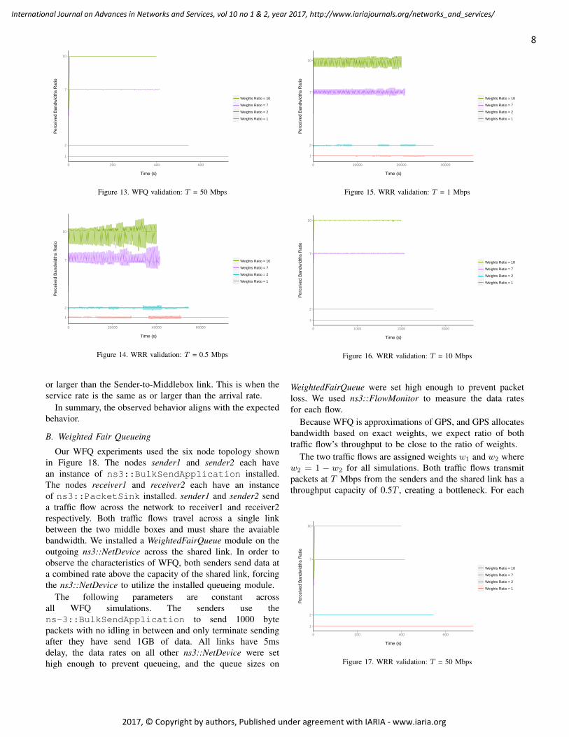
B. Weighted Fair Queueing
Our WFQ experiments used the six node topology shownin Figure 18. The nodes sender1 and sender2 each havean instance of ns3::BulkSendApplication installed.The nodes receiver1 and receiver2 each have an instanceof ns3::PacketSink installed. sender1 and sender2 senda traffic flow across the network to receiver1 and receiver2respectively. Both traffic flows travel across a single linkbetween the two middle boxes and must share the avaiablebandwidth. We installed a WeightedFairQueue module on theoutgoing ns3::NetDevice across the shared link. In order toobserve the characteristics of WFQ, both senders send data ata combined rate above the capacity of the shared link, forcingthe ns3::NetDevice to utilize the installed queueing module.
The following parameters are constant acrossall WFQ simulations. The senders use thens-3::BulkSendApplication to send 1000 bytepackets with no idling in between and only terminate sendingafter they have send 1GB of data. All links have 5msdelay, the data rates on all other ns3::NetDevice were sethigh enough to prevent queueing, and the queue sizes on
1
2
7
10
0 10000 20000 30000
Time (s)
Per
ceiv
ed B
andw
idth
s R
atio
Weights Ratio = 10
Weights Ratio = 7
Weights Ratio = 2
Weights Ratio = 1
Figure 15. WRR validation: T = 1 Mbps
1
2
7
10
0 1000 2000 3000
Time (s)
Per
ceiv
ed B
andw
idth
s R
atio
Weights Ratio = 10
Weights Ratio = 7
Weights Ratio = 2
Weights Ratio = 1
Figure 16. WRR validation: T = 10 Mbps
WeightedFairQueue were set high enough to prevent packetloss. We used ns3::FlowMonitor to measure the data ratesfor each flow.
Because WFQ is approximations of GPS, and GPS allocatesbandwidth based on exact weights, we expect ratio of bothtraffic flow’s throughput to be close to the ratio of weights.
The two traffic flows are assigned weights w1 and w2 wherew2 = 1 − w2 for all simulations. Both traffic flows transmitpackets at T Mbps from the senders and the shared link has athroughput capacity of 0.5T , creating a bottleneck. For each
1
2
7
10
0 200 400 600
Time (s)
Per
ceiv
ed B
andw
idth
s R
atio
Weights Ratio = 10
Weights Ratio = 7
Weights Ratio = 2
Weights Ratio = 1
Figure 17. WRR validation: T = 50 Mbps
8
International Journal on Advances in Networks and Services, vol 10 no 1 & 2, year 2017, http://www.iariajournals.org/networks_and_services/
2017, © Copyright by authors, Published under agreement with IARIA - www.iaria.org

module we ran sets of four simulations where w2 = 1, 12 ,17 ,
110
and T is fixed, we repeated this four times with differentdata rates T = 0.5, 1, 10, 50. In each simulation, the receiversmeasure the average throughput of both flows, R1 and R2
over 1ms intervals and the we record the ratio. All simulationsstopped after the first traffic flow had finished transmitting toprevent the experiment from recording any data that does notinclude both senders.
The results in Figures 10, 11, 12, and 13 show the ratioof throughput at the receivers remains close to the ratio ofweights. As we increase data rate across the network, themeasured ratio converges to the theoretical one.
For each flow in a correctly implemented WFQ system, thenumber of bytes served should not lag behind an ideal GPSsystem by more than the maximum packet length. In low datarates such as 0.5Mbps even one packet can make a noticeabledifference. For instance, in a GPS system when the ratio ofweights is 10, the first flow sends 10 packets and the secondflow sends 100 packets over the same time interval. However,in the corresponding WFQ system if the first flow sends 9packets, then the perceived ratio will be 11.11 instead of 10.
C. Weighted Round Robin
Our WRR experiments used the same six nodetopology used by the WFQ experiments, shown inFigure 18. ns-3::BulkSendApplication andns-3::PacketSink were installed on the same nodes, andns-3::FlowMonitor was used to collect data. In theseexperiments, we installed the WeightedRoundRobin moduleon the outgoing ns3::NetDevice across the shared link.
Similarly, each ns-3::BulkSendApplication wasprogrammed to send 1000 byte packets with no idling until1 GB of data had been sent. We kept all link delays, data rates,and queue sizes in this set of experiments unchanged from theWFQ experiments.
We collected data from these experiments using the samemethods and calcuations described in the previous sectionon WFQ. Like WFQ, WRR is an approximation of GPS,and we expect ratio of both traffic flow’s throughput to be
Figure 18. Simulated network used in WFQ and WRR validationexperiments
close to the ratio of weights. Because WRR is optimal whenusing uniform packet sizes, a small number of flows, and longconnections, we observe that WRR performs as well as WFQin approximating GPS. As expected, we can see in Figures 14,15, 16, and 17 that the measured ratio of throughput convergesto the ratio of weights as data rate increases.
VI. USAGE
As discussed in Section IV, CLASSs and their correspond-ing ACLs must be defined before the simulation can start. Inaddition to working with objects directly in their applications,users can provide this information through a text or XML file.
A. Text input configuration file
The input configuration data can be provided through a textfile. This file consists of a set of lines where each line is acommand designated to introduce an ACL or a CLASS to thesystem. These commands are simplified versions of Cisco IOScommands and should be familiar to users who have workedwith Cisco products.
Here, access-list command can be used to define asingle ACL. Figure 19 shows the syntax of the command andthe order of the parameters.
a c c e s s− l i s t a c c e s s−l i s t −i d[ p r o t o c o l ][ s o u r c e a d d r e s s ][ s o u r c e a d d r e s s m a s k ][ o p e r a t o r [ s o u r c e p o r t ] ][ d e s t i n a t i o n a d d r e s s ][ d e s t i n a t i o n a d d r e s s m a s k ][ o p e r a t o r [ d e s t i n a t i o n p o r t ] ]
Figure 19. access-list command syntax
Furthermore, class command defines a single CLASS.Weight amount can be determined using the bandwidthpercent parameter and queue size is set by queue-limit.Figure 20 demonstrates the syntax of class command and theorder of the parameters.
c l a s s [ c l a s s i d ]bandwid th p e r c e n t [ we ig h t ]queue−l i m i t [ q u e u e s i z e ]
Figure 20. class command syntax
After defining a CLASS, it is expected to be linked toan ACL. This is done through a class-map command thatmatches one CLASS with one ACL. Figure 21 provides thesyntax of class-map command.
c l a s s−map [ c l a s s i d ]match a c c e s s−group [ a c l i d ]
Figure 21. class-map command syntax
We provide a simple example here to configure a sampleWFQ system that has two classes with weights’ ratio of 7
9
International Journal on Advances in Networks and Services, vol 10 no 1 & 2, year 2017, http://www.iariajournals.org/networks_and_services/
2017, © Copyright by authors, Published under agreement with IARIA - www.iaria.org

and queue sizes of 256 packets. We define an ACL calledhighACL for the class with higher weight and another ACLcalled lowACL for the class with lower weight. highACLincludes traffic from 10.1.1.0 network with port number 80aiming to 172.16.1.0 network with the same port numbervia TCP protocol. lowACL, however, includes traffic from10.1.1.0 with port number 21 heading towards 172.16.1.0with the same port number via TCP protocol. Figure 22demonstrates the example.
a c c e s s− l i s t highACL TCP 1 0 . 1 . 1 . 0 0 . 0 . 0 . 2 5 5 eq 801 7 2 . 1 6 . 1 . 0 0 . 0 . 0 . 2 5 5 eq 80
a c c e s s− l i s t lowACL TCP 1 0 . 1 . 1 . 0 0 . 0 . 0 . 2 5 5 eq 211 7 2 . 1 6 . 1 . 0 0 . 0 . 0 . 2 5 5 eq 21
c l a s s h ighC l bandwid th p e r c e n t 0 .875 queue−l i m i t 256c l a s s lowCl bandwid th p e r c e n t 0 .125 queue−l i m i t 256c l a s s−map h ig hCl match a c c e s s−group highACLc l a s s−map lowCl match a c c e s s−group lowACL
Figure 22. A sample example demonstrating configuration of WFQ usingtext file commands
B. XML input configuration file
Alternatively, users can provide input configuration datavia an XML file where they can provide a set of ACLs tothe system using <acl_list> tag. An <acl list> tag caninclude one or multiple ACLs. Each ACL is defined usingan <acl> tag and can have one or multiple set of rules orentries defined by <entry> tags.
Similar to ACLs, CLASSs are introduced using a<class_list> tag, which is a set of CLASSs each definedby a <class> tag. Each CLASS has queue_limit andweight properties and is linked to its corresponding ACLusing acl_id attribute.
Again we provide an example of configuration of WFQ. Weuse the example that we already used in the previous sectionand show that how it can be implemented via an XML file.Figure 23 demonstrates the example.
VII. CONCLUSION AND FUTURE WORK
In order to add new functionality to ns-3, we havedesigned and implemented modules for SPQ, WFQ, andWRR. We have detailed our implementations of these wellknown algorithms and presented the reader with the means tounderstand their operation. We have validated these modulesand shared our experiment designs and results to prove theircorrectness. Utilizing the instruction and examples we havegiven, readers can write simulations that make use of ourmodules for further experimentation. The ease of configurationand use of our modules should make them attractive tools forfurther research and we look forward to seeing how otherstake advantage of our work.
There is a further oppurtunity to break these modules intoabstract components for re-use. There exist obvious sharedfunctionality between the three queues, particularly WFQand WRR. All three modules perform classification, a newclass could be implemented to handle classsification for any
<a c l l i s t ><a c l i d = ‘ ‘ highACL”>
<e n t r y><s o u r c e a d d r e s s >1 0 . 1 . 1 . 0</ s o u r c e a d d r e s s><s o u r c e a d d r e s s m a s k >0 . 0 . 0 . 2 5 5</ s o u r c e a d d r e s s m a s k><s o u r c e p o r t n u m b e r >80</ s o u r c e p o r t n u m b e r><d e s t i n a t i o n a d d r e s s >1 7 2 . 1 6 . 1 . 0</ d e s t i n a t i o n a d d r e s s ><d e s t i n a t i o n a d d r e s s m a s k >0 . 0 . 0 . 2 5 5</ d e s t i n a t i o n a d d r e s s m a s k><d e s t i n a t i o n p o r t n u m b e r >80</ d e s t i n a t i o n p o r t n u m b e r><p r o t o c o l>TCP</ p r o t o c o l>
</ e n t r y></ a c l><a c l i d = ‘ ‘ lowACL”>
<e n t r y><s o u r c e a d d r e s s >1 0 . 1 . 1 . 0</ s o u r c e a d d r e s s><s o u r c e a d d r e s s m a s k >0 . 0 . 0 . 2 5 5</ s o u r c e a d d r e s s m a s k><s o u r c e p o r t n u m b e r >21</ s o u r c e p o r t n u m b e r><d e s t i n a t i o n a d d r e s s >1 7 2 . 1 6 . 1 . 0</ d e s t i n a t i o n a d d r e s s ><d e s t i n a t i o n a d d r e s s m a s k >0 . 0 . 0 . 2 5 5</ d e s t i n a t i o n a d d r e s s m a s k><d e s t i n a t i o n p o r t n u m b e r >21</ d e s t i n a t i o n p o r t n u m b e r><p r o t o c o l>TCP</ p r o t o c o l>
</ e n t r y></ a c l>
</ a c l l i s t ><c l a s s l i s t >
<c l a s s i d = ‘ ‘ h igh Cl ” a c l i d = ‘ ‘ highACL”><q u e u e l i m i t >256</ q u e u e l i m i t><weight >0.875</ weight>
</ c l a s s ><c l a s s i d = ‘ ‘ lowCl ” a c l i d = ‘ ‘ lowACL”>
<q u e u e l i m i t >256</ q u e u e l i m i t><weight >0.125</ weight>
</ c l a s s ></ c l a s s l i s t >
Figure 23. A sample example demonstrating configuration of WFQ usingXML file
differentiated service queue. Scheduling, although differentfor each queue type, has identical interfaces and could beimplemented as a base class for differentiated service queuesto inherit from and respective their own scheduling classes.These shared classes could form the base of a frameworkfor creating additional differentiated service queue modulesin ns-3.
REFERENCES
[1] R. Chang, M. Rahimi, and V. Pournaghshband, “Differentiated ServiceQueuing Disciplines in ns-3,” In Proc. of the Seventh InternationalConference on Advances in System Simulation (SIMUL), Barcelona,Spain, November 2015.
[2] ”The ns-3 Network Simulator,” Project Homepage. [Online]. Available:http://www.nsnam.org [Retrieved: September, 2015]
[3] J. Kopena, “ns3: Quick Intro and MANET WG Implementations,”Proceedings Of The Seventy-Second Internet Engineering Task Force,Dublin, Ireland, 2008.
10
International Journal on Advances in Networks and Services, vol 10 no 1 & 2, year 2017, http://www.iariajournals.org/networks_and_services/
2017, © Copyright by authors, Published under agreement with IARIA - www.iaria.org

[4] P. Baltzis, C. Bouras, K. Stamos, and G. Zaoudis, “Implementation of aleaky bucket module for simulations in ns-3,” tech. rep., Workshop onICT - Contemporary Communication and Information Technology, Split- Dubrovnik, 2011.
[5] S. Ramroop, “Performance evaluation of diffserv networks using the ns-3 simulator,” tech. rep., University of the West Indies Department ofElectrical and Computer Engineering, 2011.
[6] Y. Qian, Z. Lu, and Q. Dou, “Qos scheduling for nocs: Strict priorityqueuing versus weighted round robin,” tech. rep., 28th InternationalConference on Computer Design, 2010.
[7] A. Parekh and R. Gallager, “A generalized processor sharing approachto flow control in integrated services networks: the single node case,”IEEE/ACM Transactions on Networking, vol. 1, no. 3, 1993, pp. 344-357.
[8] A. Demers, S. Keshav, and S. Shenker, “Analysis and simulation of a fairqueuing algorithm,” ACM SIGCOMM, vol. 19, no. 4, 1989, pp. 3-14.
[9] S. Keshav, “An Engineering Approach to Computer Networking.” Addi-son Wesley, 1998.
[10] M. Katevenis, S. Sidiropoulos, and C. Courcoubetis, “Weighted round-robin cell multiplexing in a general-purpose atm switch chip,” IEEEJournal on Selected Areas in Communications, vol. 9, no. 8, 1991.
[11] “The ns-2 Network Simulator,” Project Homepage. [Online]. Available:http://www.isi.edu/nsnam/ns/ [Retrieved: September, 2015]
[12] V. Pournaghshband, “End-to-End Detection of Third-Party MiddleboxInterference, Ph.D. Dissertation, University of California, Los Angeles,2014
[13] M. Rahimi and V. Pournaghshband, “An Improvement Mechanism forLow Priority Traffic TCP Performance in Strict Priority Queueing,” InProc. of IEEE International Conference on Computer Communicationsand Informatics (ICCCI), pp. 570, January 2016.
[14] S. Keshav, “On the efficient implementation of fair queueing,” In Journalof Internetworking: Research and Experience, volume 2, number 3,December 1991.
11
International Journal on Advances in Networks and Services, vol 10 no 1 & 2, year 2017, http://www.iariajournals.org/networks_and_services/
2017, © Copyright by authors, Published under agreement with IARIA - www.iaria.org

Pipeline Monitoring and Spillage Prevention Using Wireless Sensors and High Density Polyethylene Pipe Encasement System
Mohammed Yusuf Agetegba
College of Computer Science and Information Technology Sudan University of Science and Technology
Khartoum, Sudan email: [email protected]
Pascal Lorenz University of Haute Alsace
34 rue du Grillenbreit, Colmar - France. email: [email protected]
Abstract—Nigerian Niger Delta region is bedeviled with rampant oil spills, making it almost impossible for her indigenous people to enjoy economic activities derived from farming and fishing. Incessant oil thefts, corroded pipelines, vandalism, sabotage and extreme protests by sections of Niger Delta indigenous people are responsible for most oil spills in the region. Our proposed eco-friendly solution uses wireless motes and High Density Polyethylene Pipe System. While the former monitor attempts to vandalize encased crude oil pipelines, the latter collects crude oil seeping from corroded or damaged portions of encased steel or iron pipeline. This prevents spilled crude oil from causing ecological damage on land, rivers and seas in the region. Wireless sensors are arranged linearly within High Density Polyethylene Pipe System, linear clustering is adopted for rapid reporting within each cluster. Pipe monitoring is achieved by engaging light sensor of wireless motes, while crude oil spillage is detected and reported to mote using float switches.
Keywords—Monitoring; Sensors; Pipes; Cluster; Linear; Mote
I. INTRODUCTION
Various projects [1][2][3][12] demonstrated the ability of wireless sensors to “sense” deployed environment and transmit “sensed” data to a central data collection gateway. Data packets are transmitted using multi-hop transmission from sender to receiver. This ensures packets hops along until it reaches intended destination (usually personal area network coordinator, abbreviated as PAN). Wireless sensor nodes are arranged within clusters to optimize both packet transmission and power consumption [4].
Essentially, a wireless node is a miniaturize computer which runs on low power, a typical sensor hardware comprises of one or more sensors, a signal conditioning unit, an analog to digital conversion module (ADC), a central processing unit (CPU), Memory, a radio transceiver and an energy power supply unit [5][6]. Wireless sensors are often encased in a protective housing which offers some level of protection against physical or chemical damage.
Advances in wireless sensor’s MAC layer has made it possible for sensor nodes to operate for a year or more on a pair of AA batteries [6][7][18][19]. However, due to the high cost of removing and replacing pipes in order to access and replace spent AA batteries, our proposed deployment environment will not rely on pairs of AA batteries to power
each wireless node. Rather, power will be supplied to nodes from power banks which are strategically located along deployed pipeline route.
Figure 1. Wireless Sensor Node Architecture
Sensors nodes typically adopt IEEE 802.15.4/ZigBee
standard [8][9]. This standard introduces two types of devices within a wireless sensor network (WSN), a full-function device (FFD) and a reduced-function device (RFD). An FFD is capable of the following:
• Become a personal area network (PAN) coordinator which controls network initialization and manage the entire network.
• Become a coordinator, which removes network initialization, but retains complete management of entire network.
• Become a normal sensor device responsible for sensing deployed environment and forwarding sensed data to cluster’s PAN coordinator.
An RFD is used to perform simple tasks like connect to sensors and send collated readings to the network coordinator or PAN.
This research paper propose encasing pipelines within high density polyethylene (HDPE) pipes fitted with wireless sensors and float switches, making it easier to monitor both pipeline vandalism and oil spills.
12
International Journal on Advances in Networks and Services, vol 10 no 1 & 2, year 2017, http://www.iariajournals.org/networks_and_services/
2017, © Copyright by authors, Published under agreement with IARIA - www.iaria.org

To reduce cost, we propose using RFD sensors to both monitor ambient light and spilled crude oil within HDPE pipeline. Sensed data are forwarded via multi-hop to an FFD acting as the wireless sensor network (WSN) PAN coordinator.
This research encapsulates the effect of encasing crude oil within specially modified high density polyethylene (HDPE) pipes.
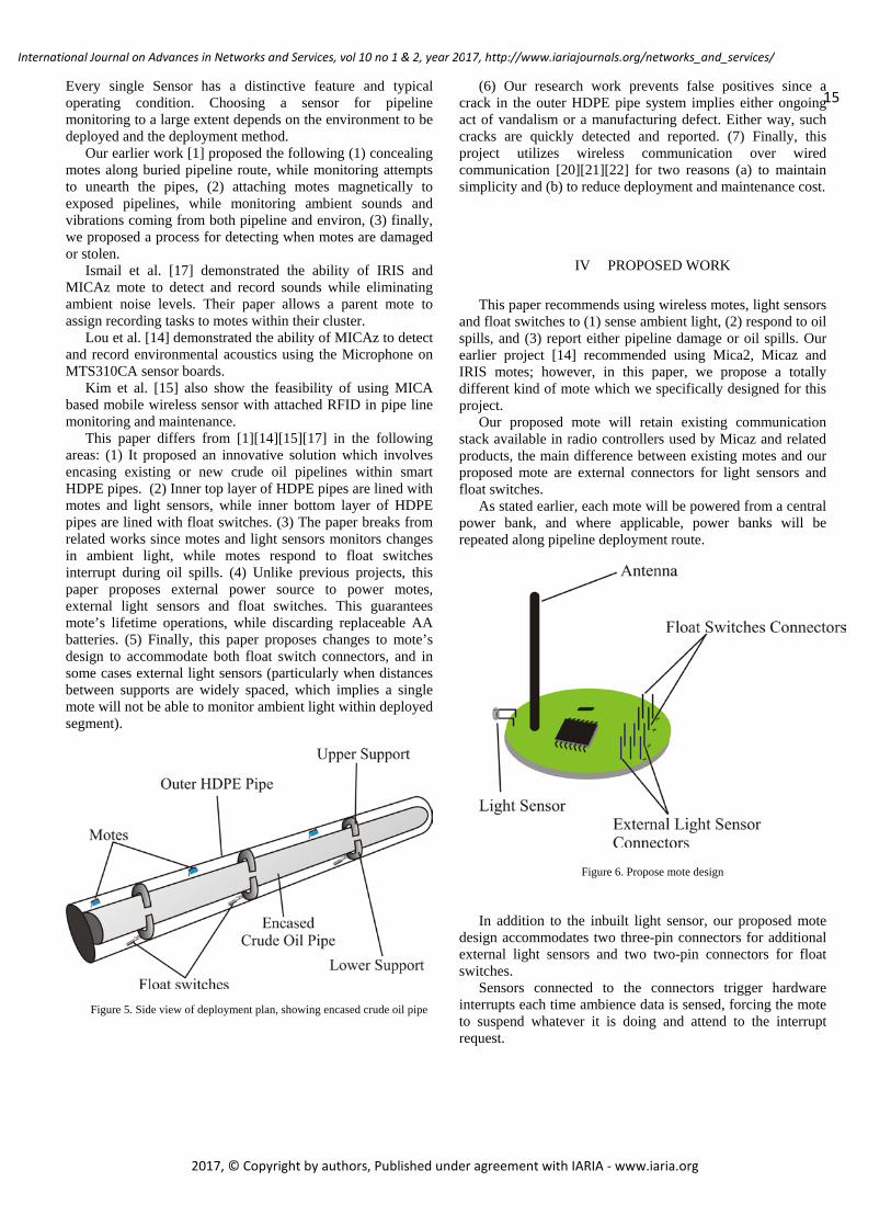
We modified the upper inner portion of the HDPE pipe to accommodate both FFD and RFD sensor (Figure 2) within separate compartments or segments. The lower portion of the pipe was equally modified to accommodate float switches and reusable spilled crude oil removal seal. The paper equally proposed powering sensors and float switches through external power banks, this ensures steady operations by eliminating periodic replacement of batteries powering each mote and requirement of opening of HDPE pipes to replace spent sensor AA batteries.
HDPE pipes were chosen for the following reasons: • Resistance to corrosive chemicals available in crude
oil • Cheaper cost of manufacturing • Fast and simple deployment options
Figure 2. Top half of HDPE pipe fitted with sensors, wires conveying power and encased pipeline supports
Figure 3. Bottom half of HDPE pipe fitted with float switches, wires conveying power and encased pipeline supports
The remaining part of this paper is organized as follows:
Section II presents background motivation behind our proposal, along with details on the corrosive nature of crude oil, and inherent benefits of using HDPE pipes to encase oil pipelines. Section III examines current state of the art research in this field, which explores various methods used to monitor pipelines for vandalism, natural disaster, and leakages. While Section IV presents our proposed work. Section V presents and discusses the simulation results. Finally, Section VI concludes the paper with pointers to further research works.
II. BACKGROUND
Generally, oil spills poses serious long-term ecological disaster in affected communities [10][1]. Oil spills occur when pipelines transporting crude oil ruptures; pipeline rupture occurs under the following circumstances: (1) rust resulting from corrosive crude oil, (2) rust as a result of aging pipes, (3) acts of vandalism and extreme economic protest (especially in places like Nigeria), and (4) equipment failure due to natural disasters (earthquakes or landslides) [10] [11].
A major challenge facing oil companies is inherent delay in detecting oil spills, such delay allow spilled crude oil to
13
International Journal on Advances in Networks and Services, vol 10 no 1 & 2, year 2017, http://www.iariajournals.org/networks_and_services/
2017, © Copyright by authors, Published under agreement with IARIA - www.iaria.org

spread further from the ruptured pipe, leading to greater ecological damage and expensive litigations/settlements.
Yarin [10] in his excellent work on crude oil corrosiveness; enumerated six components found in crude oil that makes it corrosive, these are summarized below:
• Brackish Water (Chlorides): Available in most crude oil, it contains the following chloride salts MgCI2, CaCI2 and NaCI. Preheating affected crude oil to a temperature higher than 240° F (120° C) breaks these salts down to HCI. However, HCI is only corrosive when it cools down to a temperature lower than morning dew, leading to the production of hydrochloric acid (H2S), which is highly corrosive. Listed below are various chemical degradations caused by these salts [10][11]:
CaCI2 + H2O = CaO + 2HCI HCI + Fe = FeCI2 + H2 FeCI2 + H2S = FeS + 2 HCI
• Carbon Dioxide (CO2): When CO2 mixes with
water, it produces a severely corrosive acid known as carbonic acid (H2CO3). Carbonic acid is corrosive to normal steel pipes, however, it does not affect stainless steel pipes [10][11].
• Phantom Chlorides (Organic Chlorides): These salts
decompose into HCI during preheating process. Corrosive actions triggered by these salts severely affect overhead or downstream units [10][11].
• Organic Acids: Naphthenic acid corrosion (NAC)
occurs in refiner distillation units (furnace tubes, transfer lines, sidecut piping etc). Temperatures in these areas are between 446° F and 752° F (230° C and 400° C). Naphthenic acids react with steel to produce hydrogen as shown below [10][11]:
Fe + 2 RCOOH = (RCOO) 2 + H Presence of sulfides in crude oil causes Fe (RCOO) 2 to react with H2S and produce FeS as shown below [11]: Fe (RCOO) 2 + H2S = Fes + 2RCOOH
• Sulfur: Sulfides are highly corrosive to plain and
alloy steel at temperatures higher than 466° F or (230°C), higher sulfidation occurs at higher temperatures, especially when H2S decomposes to elemental sulfur [11].
• Bacteria: Microbiologically influenced corrosion
(MIC) is widespread in oil and gas storage and transportation facilities. Sulfate reduction bacteria (SRB) are responsible for over 75% corrosion of such facilities in the US alone. SRB uses sulfate as an acceptor to create sulfide using the following reaction [10][11]:
SO42 + H2 = H2S + H2O
The foregoing reveals the possibility of oil spills occurring outside acts of vandalism. Such spills are caused when corrosive crude oil corrodes the pipeline along which it travels; this implies oil spills can happen anytime and anywhere. Hence the need to for a innovative research into what can be done to maintain the ecological balance along pipeline deployment routes. Encasing crude oil pipelines within a second protective and intelligent layer greatly reduce incidence of late detection of oil spills.
Interestingly, various HDPE pipes already convene crude oil. Tests [11] conducted by Shell International, The Hague, confirmed HDPE pipe can service pressure of up to 150 bar (2,175 psi) in temperatures of -30° C. (-22° C.) to 30° C. (86° F.). According to [11], the pipe used in this test is manufactured by Tubes d'Aquitaine, Carsac, France, and supplied as Reinforced Thermo Plastic (RTP) pipe (see image below):
Figure 4. RTP pipe consists of a primary tube in HDPE (left), several crossed layers of Aramid yarns coated with HDPE (center), and an outer layer
(right) of HDPE for external protection [13]
From the foregoing, our proposal to use HDPE pipes as encasement for existing or new crude oil pipelines is feasible.
.
III. STATE OF THE ART
Several methods have been devised in order to monitor and
report pipeline status. The most common and popular ones includes Acoustic Sensors – this employs acoustic or vibration measurement for pipeline monitoring [1][13][14][15]. Vision based systems – this is based on PIG (Pipeline Inspection Gauge) which must be inserted into the pipe. It works like image processor or laser scanner which main function is to detect leakages [13][15]. Ground penetrating radar (GPR) based systems – this is best suitable for use on environment with dry soil, but is not good for large network of pipes monitoring [13][14][15]. Fiber optic Sensors - this is suitable for present day pipeline monitoring systems, it can handle most present day pipelines issues, some of its drawbacks is the probability for redundancy and some challenges with deployment [13][16]. Multi modal underground wireless system – this uses low power, as the name implies it is meant for an underground installation, it has the advantage of camouflaging, but one of the disadvantages is that it has to be buried underground, that is a trench has to be created [13][15].
14
International Journal on Advances in Networks and Services, vol 10 no 1 & 2, year 2017, http://www.iariajournals.org/networks_and_services/
2017, © Copyright by authors, Published under agreement with IARIA - www.iaria.org
Every single Sensor has a distinctive feature and typical operating condition. Choosing a sensor for pipeline monitoring to a large extent depends on the environment to be deployed and the deployment method.
Our earlier work [1] proposed the following (1) concealing motes along buried pipeline route, while monitoring attempts to unearth the pipes, (2) attaching motes magnetically to exposed pipelines, while monitoring ambient sounds and vibrations coming from both pipeline and environ, (3) finally, we proposed a process for detecting when motes are damaged or stolen.
Ismail et al. [17] demonstrated the ability of IRIS and MICAz mote to detect and record sounds while eliminating ambient noise levels. Their paper allows a parent mote to assign recording tasks to motes within their cluster.
Lou et al. [14] demonstrated the ability of MICAz to detect and record environmental acoustics using the Microphone on MTS310CA sensor boards.
Kim et al. [15] also show the feasibility of using MICA based mobile wireless sensor with attached RFID in pipe line monitoring and maintenance.
This paper differs from [1][14][15][17] in the following areas: (1) It proposed an innovative solution which involves encasing existing or new crude oil pipelines within smart HDPE pipes. (2) Inner top layer of HDPE pipes are lined with motes and light sensors, while inner bottom layer of HDPE pipes are lined with float switches. (3) The paper breaks from related works since motes and light sensors monitors changes in ambient light, while motes respond to float switches interrupt during oil spills. (4) Unlike previous projects, this paper proposes external power source to power motes, external light sensors and float switches. This guarantees mote’s lifetime operations, while discarding replaceable AA batteries. (5) Finally, this paper proposes changes to mote’s design to accommodate both float switch connectors, and in some cases external light sensors (particularly when distances between supports are widely spaced, which implies a single mote will not be able to monitor ambient light within deployed segment).
Figure 5. Side view of deployment plan, showing encased crude oil pipe
(6) Our research work prevents false positives since a crack in the outer HDPE pipe system implies either ongoing act of vandalism or a manufacturing defect. Either way, such cracks are quickly detected and reported. (7) Finally, this project utilizes wireless communication over wired communication [20][21][22] for two reasons (a) to maintain simplicity and (b) to reduce deployment and maintenance cost.
IV PROPOSED WORK
This paper recommends using wireless motes, light sensors and float switches to (1) sense ambient light, (2) respond to oil spills, and (3) report either pipeline damage or oil spills. Our earlier project [14] recommended using Mica2, Micaz and IRIS motes; however, in this paper, we propose a totally different kind of mote which we specifically designed for this project.
Our proposed mote will retain existing communication stack available in radio controllers used by Micaz and related products, the main difference between existing motes and our proposed mote are external connectors for light sensors and float switches.
As stated earlier, each mote will be powered from a central power bank, and where applicable, power banks will be repeated along pipeline deployment route.
Figure 6. Propose mote design
In addition to the inbuilt light sensor, our proposed mote
design accommodates two three-pin connectors for additional external light sensors and two two-pin connectors for float switches.
Sensors connected to the connectors trigger hardware interrupts each time ambience data is sensed, forcing the mote to suspend whatever it is doing and attend to the interrupt request.
15
International Journal on Advances in Networks and Services, vol 10 no 1 & 2, year 2017, http://www.iariajournals.org/networks_and_services/
2017, © Copyright by authors, Published under agreement with IARIA - www.iaria.org

Each interrupt request is queued and processed one at a time. This approach ensures race conditions do not arise, especially when float switches and light sensors send event signals at the same time.
While each mote will come with its light sensor, we recommend additional connectors for external light sensors, especially where distances between segments exceeds the capabilities of a single light sensor. Similar reasoning drives the adoption of a two two-pin connectors on our proposed mote, to allow two float switches within a segment.
A segment is the space between encased pipeline supports. These supports are designed to tightly fit around encased pipes, preventing both light and crude oil from other segments from filtering in. This ensures any mote reporting changes in ambient light will send its true location info to the base station, sending accurate location enable response teams to quickly pinpoint disaster area. However, each segment is designed to allow crude oil to flow into adjacent segments via an overflow hole. This prevents the oil from reaching and the motes.
A. Mote Location Identification
We propose assigning each mote a unique identification based on pipe section and deployment segment. For example, assuming a hundred HDPE smart pipes are used to encase crude oil pipeline from Warri to Sapele (towns in the Niger Delta region of Nigeria), the following identification will be employed.
WS001001 - WS100500 Where WS represents Warri to Sapele pipeline system,
001 to 100 represents each HDPE pipe section and 001 to 500 represents identification number for each mote/segment deployed along Warri – Sapele pipeline system.
The Gateway system responsible for processing reports from motes is installed with Oracle MySQL database server [17], the database table contains the following fields:
Table I. Propose MySQL database table layout
Field Type/Length Description
Recorded Auto increment, Big Int, Primary Field
Record identification field
Moteid Varchar(10) Mote’s ID for example WS001001
Description Varchar(255) Describes each mote deployment information
Status Varchar(12) Sets mote’s status, with either “alive” or “unreachable”
Lastupdate Datetime Date and time when mote’s last pings Gateway
Motetype Varchar(6) Two values, either “Master” or “Backup”
The description field describes the location of each mote along pipeline deployment route. This approach eliminates any requirement for GPS sensors, while providing accurate location info for pipeline maintenance crew.
Enumerated below is a sample record for mote 001:
Table II. Sample record for mote 001 Recorded 1
Moteid WS001001
Description Warri Sapele pipeline system, Pipe Section 1, Segment 1. A KM from refinery east gate
Status Unreachable
Lastupdate 2016-12-11 08:10:03
Motetype Master The Status field in Table 2 above is periodically updated
by a stored procedure; this field can contain two values, namely alive or unreachable.
Lastupdate field is set whenever a mote contact the PAN Coordinator. Mote information is extracted from each mote’s source identification parameters [23] as encoded in the MAC Header.
Table III. Generic MAC Frame Format
Both sensing motes and PAN Coordinator are programmed to periodically exchange awareness information during networks Contention Access Periods (CAP), or in response to beacon signal sent by PAN Coordinator.
As stated earlier, the stored procedure on the MySQL database runs a check on the table every 24 hours and updates the status field.
Motes that failed to communicate with the PAN Coordinator within each 24 hour window are marked as unreachable by the stored procedure’s SQL commands.
Reports generated by the Gateway enable maintenance crews to either activate segment backup mote or visit mote location to ascertain why it is unreachable.
Therefore, a suggested deployment scenario encourages placing two motes within a segment - a master mote and a backup/redundant mote. Redundant motes can be remotely programmed to assume sensing operation whenever the master mote breakdown or is unreachable. Remote instruction equally reprograms redundant mote with the identification of failed master mote.
16
International Journal on Advances in Networks and Services, vol 10 no 1 & 2, year 2017, http://www.iariajournals.org/networks_and_services/
2017, © Copyright by authors, Published under agreement with IARIA - www.iaria.org

Each redundant or backup motes share similar identification with their master mote; however, the letter B is appended to differentiate each on the network. For example, backup mote for a mote with identification WS001001 is WS001001B.
B. Mote Message Forwarding
Our proposed motes uses predictive multi-hop when forwarding messages from sender to receiver. For instance mote WS001001 will predicatively send messages to WS001002, which in turn will predicatively send messages to WS001003.
Our predictive multi-hop can be succinctly summarized as: mote with identification x sends event messages to mote with identification x – 1.
Predictive message forwarding ensures the channel is always clear to forward messages between sender and receiver. This is possible when motes are appropriately spaced, ensuring mote to mote hopping and not mote to multi-mote.
Figure 7. Predictive multi-hop
C. Mote Security
Motes are required to periodically communicate with their PAN Coordinator every 24 hours. Failure in communicating implies the mote is either lost to theft, or simply damaged. D. Mote/Gateway Messaging
Proper messaging technique ensures hassle free operations amongst various technologies that make up our propose works. For example, mote status request is initiated by the central gateway to each cluster’s PAN, while pipeline related reports are initiated by monitoring motes upon positive feedback from attached sensors.
Message flow representation via process flowcharts are enumerated below.
Figure 8. Gateway status request and response flowchart
The flowchart above depicts messaging process between
gateway, PAN and mote. Cluster’s PAN reports “unreachable” only after failing to reach target mote after the third attempt. Response from PAN is used by the Gateway to update mote’s status.
Figure 9. Light Sensor interrupt handling flowchart
17
International Journal on Advances in Networks and Services, vol 10 no 1 & 2, year 2017, http://www.iariajournals.org/networks_and_services/
2017, © Copyright by authors, Published under agreement with IARIA - www.iaria.org

Figure 10. Float Switch interrupt handling flowchart Figures 9 and 10 represent process flowcharts for handling
detected events via interrupts. Interrupts requests are queued, processed (by reporting detected ambient event) and removed from queue. D. Mote/Gateway Messaging
Proper messaging technique ensures hassle free operations amongst various technologies that make up our propose works. For example, mote status request is initiated by the central gateway to each cluster’s PAN, while pipeline related reports are initiated by monitoring motes upon positive feedback from attached sensors.
E. Preventing Light Sensor False Positives
Like the Mica mote sensor boards MTS300 MTS310 our proposed sensor board uses a simple CdSe photocell, with a maximum light wavelength of 690 nm. The resistance of this photocell while exposed to light is 2 kΩ, while the off resistance, while in dark conditions is 520 kΩ [24].
Our design encapsulates the light sensor in a completely dark vacuum (the three-layered HDPE pipe completely encases the crude oil pipeline, while preventing any light from filtering in). Therefore, any light that filters in implies the protective outer HDPE pipe has been compromised, either through vandalism, weather conditions, manufacturing or installation flaw.
From the foregoing, false positives can be prevented by ensuring zero manufacturing defect and foolproof installation during deployment. E. Preventing Float Switch False Positives
Our design position float switches at the bottom of the HDPE pipe. This design ensures any leakage from the encased crude oil pipeline collects at the bottom of the HDPE pipe. As soon as sufficient crude oil has collected at the bottom of the HDPE pipe, the float switch naturally snap shut, triggering the mote’s overflow interrupt.
False positives can be prevented by the clean up crew, all they need do is ensure the float switch snaps back to the open
position after spilled crude oil has been drained from the HDPE pipe.
V SIMULATION RESULT Linear placement of motes within HDPE pipe sections
constrains the project to adopt linear cluster. However, by adopting predictive multi-hop, we believe packet loss and collusions will either be minimized or completely eliminated from the personal area network.
Moreover, since power is provided from a external power bank, it is imperative to compute the final power consumption prior to deployment
To confirm our expectations, the following simulations were conducted using OPNET 14.5:
• Network Throughput • End to end delay • Number of hops • Network Power Consumption
OPNET implements IEEE 802.15.4/ZigBee
communication protocol using the following objects: • ZigBee Coordinator • ZigBee Station • ZigBee Router • ZigBee End-device
Each ZigBee object enumerated above can function as
mobile or fixed devices. Since pipelines are fixed, we implemented our simulation using fixed ZigBee objects. Our simulation focused on the benefits of predictive hops over random hops within a linear cluster.
However, ZigBee End-devices cannot multi-hop from sender to receiver; rather they are designed to send their messages directly to their PAN ZigBee Coordinator, hence a ZigBee End-device that is not attached to a personal network ZigBee Coordinator automatically becomes an uninitialized network orphan. Therefore, this paper eventually discarded simulation results for Zigbee End-devices.
General simulation parameters are listed below: • Simulation Time: 3000 s • Packet Size: 1024 • Start Time: Different Start Time • Packet Inter Arrival Time: Constant , Mean 1.0 s • Scenario Size: 1000 x 1000 meters
A. Throughput Simulation Test Using Random Hops
This simulation examines the success rate of message
delivery within the pipeline, using one ZigBee Coordinator with five ZigBee Routers:
18
International Journal on Advances in Networks and Services, vol 10 no 1 & 2, year 2017, http://www.iariajournals.org/networks_and_services/
2017, © Copyright by authors, Published under agreement with IARIA - www.iaria.org

Figure 11. Layout of new simulation objects (ZigBee Coordinator and ZigBee Router) in OPNET Simulator
Parameters for each node are listed below:
ZIGBEE COORDINATOR 1. Name PAN 2. Network Type Mesh 3. Start Time Uniform (20, 21)
FIRST ZIGBEE ROUTER 1. Name WS001001 2. Destination PAN/Random 3. Start Time Uniform (180, 181)
SECOND ZIGBEE ROUTER 1. Name WS001002 2. Destination PAN/Random 3. Start Time Uniform (150, 151)
THIRD ZIGBEE ROUTER 1. Name WS001003 2. Destination PAN/Random 3. Start Time Uniform (120, 121)
FOURTH ZIGBEE ROUTER 1. Name WS001004 2. Destination PAN/Random 3. Start Time Uniform (90, 91)
FIFTH ZIGBEE ROUTER 1. Name WS001005 2. Destination PAN/Random 3. Start Time Uniform (60, 61)
The next set of simulation through results demonstrates the ability of nodes outside PAN coordinator coverage area to adopt multi-hop in delivery messages. We modified the Scenario size to 500 x 1500 meters to accommodate more nodes.
Figure 12. ZigBee PAN Throughput Simulation Result
Figure 13. ZigBee Router (WS001001) Throughput Simulation Result
19
International Journal on Advances in Networks and Services, vol 10 no 1 & 2, year 2017, http://www.iariajournals.org/networks_and_services/
2017, © Copyright by authors, Published under agreement with IARIA - www.iaria.org
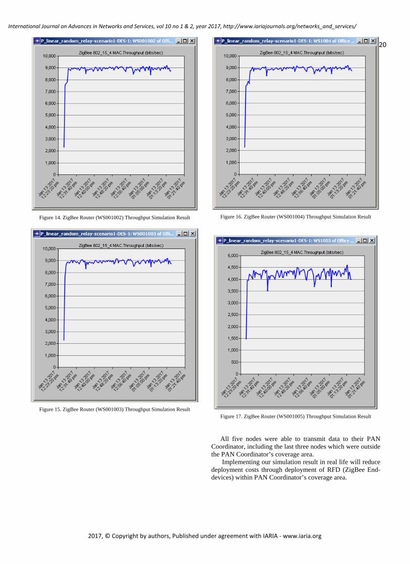
Figure 14. ZigBee Router (WS001002) Throughput Simulation Result
Figure 15. ZigBee Router (WS001003) Throughput Simulation Result
Figure 16. ZigBee Router (WS001004) Throughput Simulation Result
Figure 17. ZigBee Router (WS001005) Throughput Simulation Result
All five nodes were able to transmit data to their PAN Coordinator, including the last three nodes which were outside the PAN Coordinator’s coverage area.
Implementing our simulation result in real life will reduce deployment costs through deployment of RFD (ZigBee End-devices) within PAN Coordinator’s coverage area.
20
International Journal on Advances in Networks and Services, vol 10 no 1 & 2, year 2017, http://www.iariajournals.org/networks_and_services/
2017, © Copyright by authors, Published under agreement with IARIA - www.iaria.org

However, a FFD (ZigBee Router) will be deployed close to PAN Coordinator coverage boundary or perimeter. This placement allows nodes outside the coverage zone to route their requests through the borderline FFD. B. End to End Delay Simulation Results
End to end delay simulation results displays the time it takes for transmitted packets from source node to reach destination node. Higher end to end delay results may indicate problems in the network deployment plan.
Figure 18. ZigBee Coordinator (PAN) End to End Simulation Result
Figure 19. ZigBee Router (WS001001) End to End Simulation Result
Figure 20. ZigBee Router (WS001002) End to End Simulation Result
Figure 21. ZigBee Router (WS001003) End to End Simulation Result
Figure 22. ZigBee Router (WS001004) End to End Simulation Result
21
International Journal on Advances in Networks and Services, vol 10 no 1 & 2, year 2017, http://www.iariajournals.org/networks_and_services/
2017, © Copyright by authors, Published under agreement with IARIA - www.iaria.org
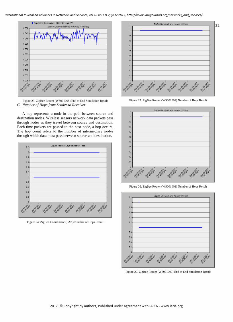
Figure 23. ZigBee Router (WS001005) End to End Simulation Result C. Number of Hops from Sender to Receiver
A hop represents a node in the path between source and destination nodes. Wireless sensors network data packets pass through nodes as they travel between source and destination. Each time packets are passed to the next node, a hop occurs. The hop count refers to the number of intermediary nodes through which data must pass between source and destination.
Figure 24. ZigBee Coordinator (PAN) Number of Hops Result
Figure 25. ZigBee Router (WS001001) Number of Hops Result
Figure 26. ZigBee Router (WS001002) Number of Hops Result
Figure 27. ZigBee Router (WS001003) End to End Simulation Result
22
International Journal on Advances in Networks and Services, vol 10 no 1 & 2, year 2017, http://www.iariajournals.org/networks_and_services/
2017, © Copyright by authors, Published under agreement with IARIA - www.iaria.org
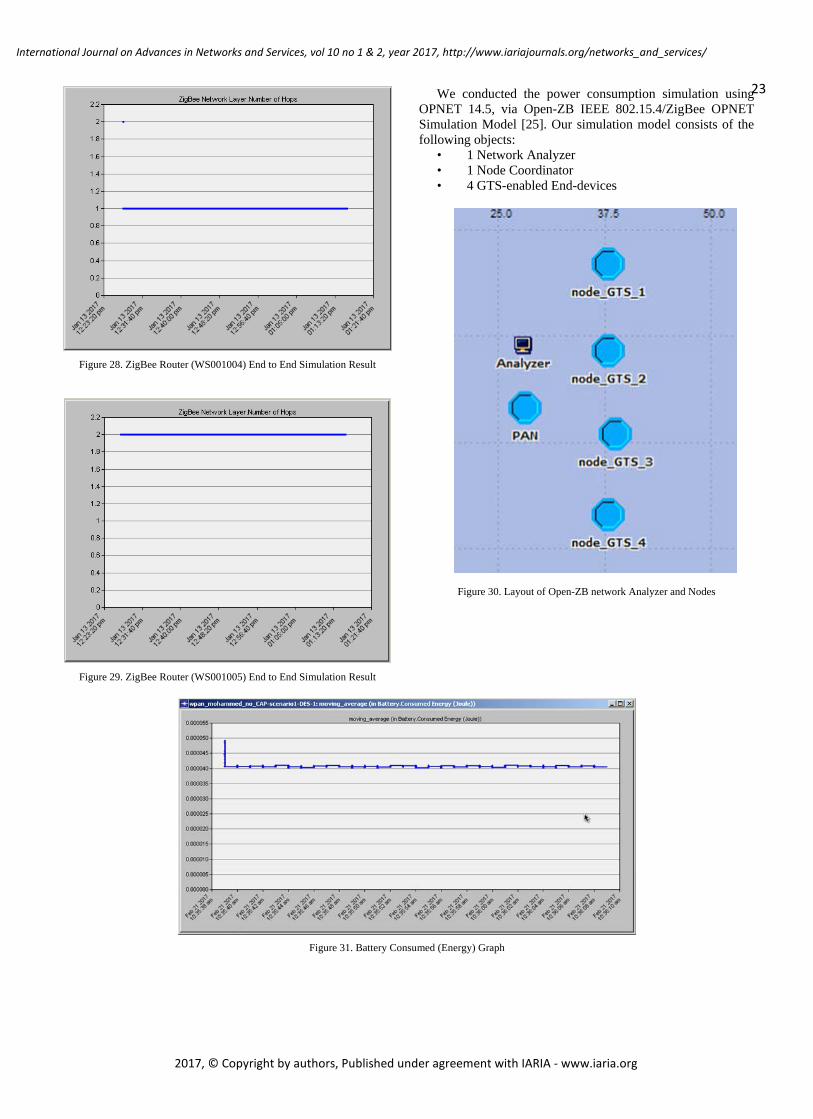
Figure 28. ZigBee Router (WS001004) End to End Simulation Result
Figure 29. ZigBee Router (WS001005) End to End Simulation Result
We conducted the power consumption simulation using
OPNET 14.5, via Open-ZB IEEE 802.15.4/ZigBee OPNET Simulation Model [25]. Our simulation model consists of the following objects:
• 1 Network Analyzer • 1 Node Coordinator • 4 GTS-enabled End-devices
Figure 30. Layout of Open-ZB network Analyzer and Nodes
Figure 31. Battery Consumed (Energy) Graph
23
International Journal on Advances in Networks and Services, vol 10 no 1 & 2, year 2017, http://www.iariajournals.org/networks_and_services/
2017, © Copyright by authors, Published under agreement with IARIA - www.iaria.org

The energy consumption graph in Figure 31 reveals high energy consumption at the start of the simulation; however, this balances out as the simulation proceeds. This implies more energy is consumed when the network initializes and less is consumed when the network is fully operational.
VI CONCLUSION AND FUTURE WORK
Messages between sender and receiver within a linear cluster depend on multiple hops, which is determined by the number of nodes between sender and receiver (as demonstrated by our simulation results).
Moreover, the advantages of predictive multi-hops within a pipe system is enormous, since it prevents nodes belonging to pipeline Segment A from communicating with Segment B or Z Coordinator, especially if such Coordinators are within range as a result of pipeline meandering downhill or around a bend.
Our future work is deployment of our proposal using live motes specially manufactured to our requirements. We believe a successful deployment will create demand, giving rise to a thriving industry, especially in countries grappling with incessant oil spills. Finally, the environmental benefits of this project should reduce oppositions to crude oil pipeline construction along environmentally delicate routes.
REFERENCES
[1] M. Y Agetegba and P. Lorenz “Using Sensor Technology to Monitor
and Report Vandalized Pipelines” INNOV 2016: The Fifth International Conference on Communications, Computation, Networks and Technologies, August 2016, pp. 1 - 6
[2] N. Bhavana, S. Anuradha, K. Sanjay, and P. Vinod “Energy Efficient
MAC Protocols for Wireless Sensor Networks: A Survey” Computer Science and Engineering Survey Vol.2, No. 3, August 2011, pp. 122-129.
[3] L. M. L. Oliveira and J. J. P. C. Rodrigues, “Wireless Sensor Networks:
a Monitoring” Journal of Communications, April 2011, Vol. 6, No. 2, pp. 3-16.
[4] L. M. L. Oliveira, J. J. P. C. Rodrigues, A. G. F. Elias, and B. B. Zarpelão, “Ubiquitous monitoring solution for Wireless Sensor Networks with push notifications and end-to-end connectivity” 2014 pp. 1 - 2.
[5] G. Han, X. Jiang, A. Qian, J. J. .P. C. Rodrigues, and L. Cheng, “A Wireless Comparative Study of Routing Protocols of Heterogeneous Sensor Networks” Research Article, June 2014, pp. 1-3.
[6] E. Romero, A. Araujo, J. Blesa, and O. Nieto-Taladriz “Developing Cognitive Strategies for Reducing Energy Consumption in Wireless Sensor Networks” The Second International Conference on Advances in Cognitive Radio, COCORA 2012, pp. 64 – 65.
[7] O. Diallo, J. J. P. C. Rodrigues, and M. Sene, “Real-time data Management on wireless sensor networks: A survey” Journal of Network and Computer Applications, www.elsevier.com/locate/jnca December 2011, pp.2 – 8.
[8] V. N. G. J. Soares and J. J. P. C. Rodrigues, “Cooperation in DTN-Based Network Architectures” V2-05, April 2011, pp. 103 – 107.
[9] K. Lin, J. J. P. C. Rodrigues, H. Ge, Naixue Xiong, and X. Liang
“Energy Efficiency QoS Assurance Routing in Wireless Multimedia Sensor Networks“, IEEE Systems Journal, Vol. 5, December 2011 pp.1-3.
[10] Mehdi Yari. “The 6 Corrosive Components That Can Be Found in Crude Oil” Corrosionpedia, August 21, 2015. https://www.corrosionpedia.com/2/1424/corrosion/the-6-corrosive-components-that-can-be-found-in-crude-oil
[11] Tests confirm polyethylene pipe for high-pressure oil, gas service. http://www.ogj.com/articles/print/volume-94/issue-37/in-this-issue/general-interest/tests-confirm-polyethylene-pipe-for-high-pressure-oil-gas-service.html. Oil and Gas Journal, 1996
[12] S. A. Ahlam and A. Manal “Medium Access Control Protocols for
Wireless Sensor Networks Classifications and Cross-Layering” Science Direct, Procedure Computer Science, www.ScienceDirect.com, ICCMIT, 2015, pp. 2-13.
[13] A. M. Sadeghion, N. Metje, D. N. Chapman, and C. J. Anthony “Smartpipes: Smart Wireless Sensor Networks for Leak Detection In Water Pipelines” Journal of Sensor and Actuator Networks, February 2014, pp. 1-15.
[14] L. Luo, Q. Cao, C. Huang, T. Abdelzaher, John A. Stankovic, and M. Ward, “EnviroMic: Toward Cooperative Storage and Retrieval in Audio Sensor Networks”, 2009, pp. 1- 22
[15] J. Kim, G. Sharma, N. Boudriga, and S. S. Iyengar “SPAMMS: A Sensor-based Pipeline Autonomous Monitoring and Maintenance System” IEEE Explore, 2010, pp.2-11.
[16] M. Alnuem “Performance Analysis of Node Placement in Linear Wireless Sensor Networks” Journal of Emerging Trends in Computing and Information Sciences, January 2014, Vol. 5, No. 1, pp.1 – 8
[17] M. F. F. Bin Ismail and Wai Yie “Acoustic Monitoring System Using Wireless Sensor Networks” International Symposium on Robotics and Intelligent Sensors, 2012, pp. 2-7.
[18] C. Pandeeswaran, N. Pappa, and S.G. Jayesh” Hybrid MAC Protocol for Wireless Sensor Networks used in Time Critical Applications” Computer Science and Information Technology, 2014, pp. 3- 9.
[19] M. Lujuan, L. Henry, and L. Deshi “Hybrid TDMA/CDMA MAC Protocol for Wireless Sensor Networks” Journal of Network, Vol. 9, No.10, October 2014, pp. 2665 – 2673.
[20] Aubrey Kagan “Combining power and data wires, Part 1”. May, 2015 http://www.embedded.com/electronics-blogs/without-a-paddle/4439353/Combining-power-and-data-wires--Part-1
[21] Paul Pickering “Power & Signal Over A Single Wire Do More With Less”. May, 2015. http://www.eetimes.com/author.asp?section_id=36&doc_id=1326167&
[22] Wikipedia “Highway Addressable Remote Transducer Protocol” https://en.wikipedia.org/wiki/Highway_Addressable_Remote_Transducer_Protocol
[23] RF Wireless World “Zigbee MAC layer frames”. 2012. http://www.rfwireless-world.com/Tutorials/Zigbee-MAC-layer-frame-format.html
[24] Crossbow Technologies “MTS/MDA Sensor Board Users Manual Revision B, June 2006”
[25] Petr Jurcik Open-ZB IEEE 802.15.4/ZigBee OPNET Simulation Model. http://www.open-zb.net/wpan_simulator.php
24
International Journal on Advances in Networks and Services, vol 10 no 1 & 2, year 2017, http://www.iariajournals.org/networks_and_services/
2017, © Copyright by authors, Published under agreement with IARIA - www.iaria.org
Indoor Localization based on Principal Components and Decision Trees in IEEE
802.15.7 Visible Light Communication Networks
David Sánchez-Rodríguez1,2, Itziar Alonso-González1,2, Carlos Ley-Bosch1,2, Javier Sánchez-Medina3, Miguel
Quintana-Suárez1 and Carlos Ramírez-Casañas1,2
Department of Telematics Engineering1
Institute for Technological Development and Innovation in Communications2
Institute for Cybernetics3
University of Las Palmas de Gran Canaria
e-mail: {david.sanchez, itziar.alonso, carlos.ley, javier.sanchez, mangel.quintana, carlos.ramirez}@ulpgc.es
Abstract - Indoor positioning estimation has become an
attractive research topic due to the growing interest in
location-aware services. Research works have been proposed
on solving this problem by using wireless networks.
Nevertheless, there is still much room for improvement in the
quality of the proposed classification or regression models, i.e.,
in terms of accuracy or root mean squared error (RMSE). In
the last years, the emergence of Visible Light Communication
brings a brand new approach to high quality indoor
positioning. Among its advantages, this new technology is
immune to electromagnetic interference, and also, the variance
of the received optical power is smaller than other RF based
technologies. In this paper, we propose a fingerprinting indoor
location estimation methodology based on principal
components analysis (PCA) and decision trees as classification
learner. The proposed localization methodology is based on the
received signal strength from a grid of emitters multiple. PCA
is used to transform all of that features into principal
components, consequently reducing the data dimensionality,
improving the interpretability of the resulting tree models and
the overall computational performance of the proposed system.
Along with the proposed method, we also share experimental
results derived from the received signal strength values
obtained from an IEEE 802.15.7 simulator developed by our
research group. Results show that the system accuracy is
slightly improved by range 1%-10% and the computation time
by range 40%-50%, as compared to the system in which PCA
is not carried out. The best tested model (classifier) yielded a
95.6% accuracy, with an average error distance of 2.4
centimeters.
Keywords - Indoor Localization; Visible Light
Communication; Decision Trees; Principal Components
Analysis; Received Signal Strength.
I. INTRODUCTION
The present paper expands on the indoor localization system described in the original paper [1] proposing the use of principal components analysis (PCA) to improve the system accuracy while reducing the computational cost and carrying out some enhanced experiments.
Indoor localization has gained considerable attention over the past decade due to the emergence of numerous location-aware services. These new services have made it possible to use applications capable of sensing their location
and dynamically adjusting their settings and functions [2]. Many indoor localization approaches based on globally deployed radiofrequency systems, such as Wireless Local Area Networks (WLAN), Bluetooth and Ultra-Wide Band (UWB), have been proposed, mainly because of their low cost and mature standardization state. Nevertheless, they usually deliver an accuracy of up to two meters, since hindered by multipath propagation [3]. On the other hand, Visible Light Communication (VLC) is experiencing a growing interest due to improvements in solid state lighting and a high demand for wireless communications. VLC can offer a higher positioning accuracy [4] mainly because of two reasons: this kind of networks is not affected by electromagnetic interferences and the received optical power is more stable than radio signals and can be accurately known. For example, authors in [5] proposed a system with a positioning error about 10 centimeters using a location code and a spatial power distribution map where the received signal strength (RSS) measurements are gathered 5 centimeters separation from each other.
In this paper, we propose an indoor location estimation method based on an ensemble model of decision trees, yielding and optimal tradeoff between accuracy (high) and variance (low), and the added value of being computationally efficient. In order to achieve this tradeoff, PCA is proposed to transform RSS features of a VLC network into principal components, consequently reducing the data dimensionality and improving the computational cost of the system. The main novelty of this work comes from the fact that the positioning systems based on decision trees and principal components have a lower computational complexity and high accuracy. Additionally, the proposed methodology is also novel in the use decision trees and principal components in IEEE 802.15.7 VLC networks for indoor location estimation.
The rest of the paper is organized as follows. Section II summarizes state of the art. In Section III, we describe our simulator that implements the IEEE 802.15.7 VLC standard. Next, in Section IV, we describe the ensemble model of decision trees used for VLC indoor location estimation. Section V describes the two phases of our indoor positioning method based on an ensemble model of decision trees where PCA is considered. In Section VI, we show experimental results that demonstrate the high accuracy of our approach
25
International Journal on Advances in Networks and Services, vol 10 no 1 & 2, year 2017, http://www.iariajournals.org/networks_and_services/
2017, © Copyright by authors, Published under agreement with IARIA - www.iaria.org

and its low computational complexity. Finally, we sum up the conclusions and we present the future work.
II. STATE OF THE ART
Indoor positioning techniques for VLC are mainly
classified into two groups based on geometric properties:
lateration and angulation [6]. Lateration techniques estimate
the target location by measuring distances from the receiver
to multiple LEDs base stations with known coordinates. The
distances can be estimated involving the time of arrival
(TOA), time difference of arrival (TDOA) and RSS
measurements. On the other hand, with angulation
techniques or angle of arrival (AOA) the target location is
estimated by measuring angles to multiple base stations.
Nevertheless, these techniques often require additional
hardware, time synchronization between emitter and
receiver, knowing every base station coordinates and extra
computation. A third kind of location techniques are the so called
fingerprinting techniques, that combined with VLC can be an alternative to the aforementioned because they estimate positioning by matching online measured data with pre-measured location-related data, such as RSS. Hence, just RSS information is needed and extra sensors are unnecessary. As a matter of fact, fingerprinting is one of the most commonly used techniques for RF indoor location [7].
Localization based on fingerprinting is usually carried out in two phases. The first phase (off-line phase) consists on the sampling RSS measurements for every emitter and each reference location (VLC receiver). With that samples as training set, a positioning model is learned using a particular machine learning technique. During the second phase (on-line phase), the particular receiver position is estimated by using the learned model and the new RSS measurements.
Learned techniques based on decision trees are widely used in classification problems, and are often used in indoor localization. A decision tree is a sequence of branching operations based on comparisons of RSS values for each feature in the dataset. Depending on the training dataset size and the number of features (emitters or principal components), the depth of the tree can be high, and hence, the number of conditions to be evaluated could influence energy savings. Nevertheless, its computational complexity is considerably lower than the number of floating-point multiplication CPU cycles, where experimental results indicate that decimal64 multiplication with binary integer decimal (BID) encoding takes an average of 117 cycles using Intel’s BID library [8]. Since no floating-point multiplication takes place to predict the location using decision trees, the computational complexity of our system is O(1). The latter is an extremely important characteristic if the localization system is designed for portable devices, where both processor power and energy availability are constrained. Hence, factors such as the battery power, computation cost, and the memory size need to be jointly considered. Thus, the reduction of the data dimensions leads to a decrease in the computational complexity. In addition, the performance can
be further enhanced when the discarded information is redundant noise [9].
PCA is one of the most widely used techniques to carry out the reduction of the data dimensions. The central idea of PCA is to reduce the dimensionality of a dataset in which there are a large number of interrelated variables, while retaining as much as possible of the variation present in the dataset. This reduction is achieved by transforming to a new set of variables, the principal components, which are uncorrelated, and which are ordered so that the first few retain most of the variation present in all the original variables [10].
Regarding to indoor localization, authors in [9] proposed a novel approach based on PCA which transforms RSS into principal components such that the information of all access points (APs) is more efficiently utilized. Instead of selecting APs for the positioning, the proposed technique changes the elements with a subset of principal components improvement of accuracy and reduces the online computation. The proposed approach delivers a significantly improved accuracy. The results show that the mean error is reduced by 33.75% and the complexity is decreased by 40%, as compared to the existing techniques.
On the other hand, in 2011, Institute of Electrical and Electronic Engineers (IEEE) published the IEEE 802.15.7 standard, which defines Physical (PHY) and Medium Access Control (MAC) layers for short-range wireless optical communications using visible light [11]. Within the last few years, many studies on VLC based positioning have been published. Nevertheless, to the best of our knowledge, to this date there is no any published indoor positioning research using this standard.
With the present work, our contribution is the following: we propose an ensemble model of decision trees based indoor positioning methodology, built of principal components from RSS, together with some promising results. We have carried out a wide experimentation and present results showing the achieved high accuracy and low computational complexity. Furthermore, we make use of the IEEE 802.15.7 standard on VLC to obtain RSS values, which may be a useful piece of information for other researchers and practitioners at this stage of (un)deployment of such standard.
III. SIMULATION MODEL BASED ON IEEE 802.15.7
We built our simulator using OMNET++ [12] simulation framework from the model developed by [13] designed for sensor networks based on the IEEE 802.15.4 standard, due to the similarities existing between IEEE 802.15.7 and IEEE 802.15.4 architectures.
OMNeT++ provides built-in support tools not only for simulating, but also for the analysis and visualization of simulation results. Several data can be chosen for simulation results, such as throughput, delay, packet loss and RSS.
The developed simulation model has been designed with the following premises:
- IEEE 802.15.7 star topology has been chosen, due to its importance and wide range of applications.
26
International Journal on Advances in Networks and Services, vol 10 no 1 & 2, year 2017, http://www.iariajournals.org/networks_and_services/
2017, © Copyright by authors, Published under agreement with IARIA - www.iaria.org

- For the MAC layer, we opted to use the superframe structure; since it allows the use of both contention (CAP) and no contention (CFP) access methods. In addition, the use of the superframe enables devices to enter the energy save state during the idle period.
- A VLC Personal Area Network (VPAN) identifier is assigned to each emitter in order to identify each coordinator (LED lamp).
Next subsections describe the most important features in our simulator, for a better comprehension of the presented results.
A. Optical channel model
The transmission medium is modeled as free space without obstacles. We chose the directed line of sight (LOS) link configuration to model the optical signal propagation, requiring a LOS between each device and the coordinator. We have considered only the direct component of the received signal to calculate the received power, despising the possible influence of reflections.
Frequency response of optical channel is relatively flat near Direct Current (DC), so the most important quantity for characterizing this channel is the DC gain H(0) [14], which relates the transmitted and received optical average power, see (1):
Pr = H(0) • Pt (1)
In VLC, received power can be expressed as the sum of LOS and non-LOS components. In directed LOS links, the DC gain can be computed fairly accurately by considering only the direct LOS propagation path. According to the results presented in [15], at least 90% of total received optical power is direct light in VLC when using a receiver field of view (FOV) of 60 degrees. Figure 1 shows an example of a directed LOS link.
An optical source can be modeled by its position vector,
a unit-length orientation vector t, transmission power Pt and a radiation intensity pattern I(θ,m) emitted in direction θ.
The m parameter is the mode number of the radiation lobe, which specifies the directionality of the source, and is related to the transmitter half power angle θ1/2. Similarly, a receiver
is defined by its position, orientation r, photo detector area A, and FOV (ψc). The angle formed between the optical
incident signal and the orientation vector r is called the incident angle ψ. The maximum incident angle defines the receiver FOV.
Considering LOS propagation path, the DC gain can be calculated according to [14] as (2):
H(0)=(m+1)•cosm(θ)•A•Ts(ψ)•G(ψ)•cos(ψ)/(2πd2), 0≤ ψ ≤ ψc
H(0)=0, ψ> ψc (2)
Ts(ψ) is the optical filter signal transmission coefficient, G(ψ) is the optical concentrator gain, d is the distance between transmitter and receiver.
The adopted optical channel model facilitates reaching high transmission speeds, since the effects of multipath distortion on the optical signal are not considered. Considering only the direct component of the signal has the additional benefit of improving the efficiency of the implemented simulation model. The computational load required to run simulations of scenarios with multiple nodes including the functionality of different layers of the architecture is reduced significantly.
To ensure the validity of our implemented model, we have configured all optical receivers using a 60 degrees FOV value (ψc).
TABLE I. PHY LAYER PARAMETERS
Parameter Value
Transmission rate 1.25 Mbps
Optical clock rate 3.75 MHz
Coordinator optical transmission power (Pt) 15 W
Half Power Angle θ1/2 60o
Field of Vision (ψc) 60o
Photo detector area (A) 100 mm2
Photo detector responsivity (R) 0.54 A/W
Optical concentrator gain ( G(ψ)) 15
Optical filter transmission coefficient (Ts(ψ)) 1
B. PHY layer simulation parameters
Table I shows the main configuration parameters of
PHY layer used in all simulation scenarios. We selected the
PHY II operating mode, intended for both indoor and
outdoor environments, using MCS-ID number 16, since
support for the minimum clock and data rates for a given
PHY is mandatory.
Because of the optical channel model used, transmitters'
directivity is characterized by its half power angle, θ1/2
while receivers' directivity is defined by its FOV. According Figure 1. Directed LOS link configuration.
27
International Journal on Advances in Networks and Services, vol 10 no 1 & 2, year 2017, http://www.iariajournals.org/networks_and_services/
2017, © Copyright by authors, Published under agreement with IARIA - www.iaria.org

to [16], both parameters are assigned a value of 60 degrees,
to ensure validity of the implemented channel model, since
the calculation of received optical power takes in account
only the direct component of the signal.
In order to simplify the calculation process of the model,
the values used for the concentrator gain (G(ψ)) and the
transmission coefficient of the optical filter (Ts(ψ)) are set
up as constant values, so they do not depend on the angle of
incidence ψ.
The rest of the values selected to characterize VLC
transmitters and receivers are commonly used values in
literature, similar to those used in [17][18].
IV. ENSEMBLE MODEL OF DECISION TREES
Indoor positioning has been a very active research area where several data mining techniques have proved useful to extract knowledge from raw data [19][20]. To solve this problem, in this paper we propose a general approach based on a classifier built as an ensemble model of decision trees.
Decision trees build classification models in the form of a tree structure. In general, they can handle both categorical and numerical data. A decision tree has internal nodes and leaf nodes. An internal node includes a condition or function of any feature of the dataset, which breaks down the dataset into several subsets, corresponding to two or more branches. Each leaf is assigned to a class, representing the classification decision. For instance, in the location problem, the received optical power from luminaries is used in the internal node conditions, and the locations or reference points are used in the leaf nodes. Samples are classified by navigating from the root of the tree down to a leaf, according to the outcome of the condition or function along the path [21].
On the other hand, ensemble models are methods that combine the capabilities of multiple models to achieve better prediction accuracy than any of the individual model could do on its own. Ensemble methods generate multiple base models, and the final prediction is produced as the result of a combination of them, in some appropriate manner, from the prediction of each base model. For instance, the output of each base model is weighted. The success of the ensemble model is based on the ability of generating a set of base models that make errors that are as uncorrelated as possible.
In our indoor localization method, we use a weak classifier based on the C4.5 algorithm [22] to generate a decision tree as a base model. Then, the adaptive boosting (AdaBoost) algorithm [23] is used to build an ensemble model based on previous base models, that is a location estimation model formed by multiple weighted decision trees. AdaBoost aims at improving the accuracy of the weak learner, by concentrating in the samples incorrectly classified by that one. In a previous work, we demonstrated that this combination of machine learning techniques provides excellent results for indoor localization when it is used in WLAN networks [24].
V. INDOOR LOCALIZATION METHOD
In this section, we describe our positioning method based on an ensemble model of decision trees, and it is divided into two phases. The first phase is the training phase (off-line phase). Coordinators send beacon frames and RSS samples are collected at reference locations (receivers) to build a dataset. From this dataset, the ensemble model is built. The second stage is the test phase (on-line phase) where a receiver infers its position by using the online RSS observations
A. Training phase
In this phase, we aim at building an ensemble model of decision trees using the RSS measurements dataset as training set. Several simulations are carried out at each reference location to calculate different values of RSS. Each simulation is performed with a random orientation vector of each receiver to obtain different values. RSS data are denoted by φi,j(τ) and indicate the τ-th RSS value measured from i-th coordinator at the j-th receiver. The dataset can be
represented by as in (3):
𝜔 = (
𝜑1,1[𝜏] ⋯ 𝜑1,𝑅[𝜏]
⋮ ⋱ ⋮𝜑𝐴,1[𝜏] ⋯ 𝜑𝐴,𝑅[𝜏]
) (3)
A is the number of coordinators, R is the number of
receivers or reference locations, τ = 1, ..., N is the index of RSS samples and N is the number of RSS samples at each reference location.
When principal component analysis is used to reduce the
data dimensionality, the dataset can be represented by as in (4):
𝜔 = (
𝜑1,1[𝜏] ⋯ 𝜑1,𝑅[𝜏]
⋮ ⋱ ⋮𝜑𝑃𝐶,1[𝜏] ⋯ 𝜑𝑃𝐶,𝑅[𝜏]
) (4)
φi,j(τ) is transformed data and indicate the τ-th value
transformed from i-th principal component at the j-th receiver, and PC is the number of principal components.
After that, once that dataset of the environment is compiled, an ensemble model of decision trees is built using boosting technique.
B. Test phase
In this phase, a dataset formed by a RSS sample from
each coordinator, or its transformation if principal
component analysis is used, is taken as input of ensemble
model of decision trees to infer the current location. Using
similar notations, the online measurements can be
represented as in (5):
28
International Journal on Advances in Networks and Services, vol 10 no 1 & 2, year 2017, http://www.iariajournals.org/networks_and_services/
2017, © Copyright by authors, Published under agreement with IARIA - www.iaria.org

𝜔𝑟 = (
𝜑1,𝑟
⋮𝜑𝐴/𝑃𝐶,𝑟
) (5)
The location r is unknown.
VI. EXPERIMENTAL RESULTS
In this section, we describe the test environment, and we evaluate the impact of using principal component on the performance of indoor location estimation system. In addition, the accuracy and the computational cost of our system are evaluated.
Experiments were focused to determine the location method accuracy and the computational complexity. The error is the expected distance from the misclassified instance and the real location. The error is calculated by the Euclidean distance between these points, and the arithmetic mean was computed from the results of the experiments. Being a classification problem, an error simply means that a receiver was estimated to be in a wrong positioning cell, in the receiver’s grid. All experiments were carried out on an Intel Core i7 3.2 GHz/32 GB RAM non-dedicated Windows machine.
All experiments have been built using the API Weka software [25]. Weka is an open source collection of machine learning algorithms for data mining tasks, more specifically data preprocessing, clustering, classification, regression, visualization and feature selection.
A. Test Environment
Our method was tested in a simulation environment that models a 4 by 4 by 3 meters room. Two scenarios were implemented varying the number of receivers. Scenario 1 is shown in Fig. 2. This environment consists of 16 coordinators or LED lamps (red triangles) configured as 4 x 4 grids placed 1 meter apart from each other on the ceiling. On the lower part, we set up 100 receivers (blue circles) in a 10 x 10 grid configuration, with a 36 centimeters separation from each other. Scenario 2 uses the same number of
coordinators, but we set up 361 receivers in a 19 x 19 grid configuration with a 20 centimeters separation from each other. In order to consider different distances between receivers and coordinators, in both scenarios the receivers plane is set up at three different heights: 75, 100 and 125 centimeters from the floor. Receivers orientation was randomly produced for each simulation as follows: they are pointing out to the ceiling with an initial orientation vector [0,0,1] and a random (-0.2,0.2) offset is applied to each axis in each simulation. Thus, each receiver has a different orientation in each simulation.
Eleven simulations were performed on each three vertical layers. One RSS measurement was estimated at each receiver and simulation. This leads to 3.300 RSS and 11.913 RSS measurements for Scenarios 1 and 2, respectively. Fig. 3 shows the received optical power (lux) at 1 meter from the floor with sixteen coordinators. As it can be seen there is enough lighting to receive the beacon frame in every reference location. The simulation parameters are specified in Table 1.
B. Data Transformation using PCA
In order to transform the RSS dataset into principal
components weka.attributeSelection.PrincipalComponents
algorithm was used in conjunction with a Ranker search
(implemented in Weka by weka.attributeSelection.Ranker
class). Dimensionality reduction is accomplished by
choosing enough eigenvectors to account for 95% of the
variance in the original data. For both scenarios six principal
components were obtained. Eigenvectors for Scenario 1 are
shown in Table II, where PC1…6 denotes each principal
component and L1...16 corresponds to each LED lamp.
Similar eigenvectors are obtained for Scenario 2.
C. Analysis of the Training Dataset Size
The size of the training dataset is an important parameter
for the performance and the building time of each model
Figure 2. Scenario 1: 16 coordinators and 100 receivers.
Figure 3. Distribution of the received optical power at 1 meter
from the floor.
29
International Journal on Advances in Networks and Services, vol 10 no 1 & 2, year 2017, http://www.iariajournals.org/networks_and_services/
2017, © Copyright by authors, Published under agreement with IARIA - www.iaria.org

based on decision trees. A large-sized training dataset can
provide better accuracy to predict the correct location, but
too much data can increase the elapsed time to build the
model considerably. In order to test the robustness of the
method, different training dataset sizes were used, from
10% to 90% of the whole dataset. For the validity of
experimental results, the experiments were performed 100
times, each time selecting the training and testing data after
randomizing dataset, picking the same proportion of
samples at each class (stratified split). Also, some
experiments were carried out using 10-fold cross-validation. The classification trees were created by the C4.5
algorithm (implemented in Weka by the classifier class: weka.classifiers.trees.J48). The boosting method used was the metalearning AdaBoostM1 algorithm implemented by the Weka classifier class weka.classifiers.meta.AdaBoostM1 with number of iterations equal to 10.
Table III and Table IV for Scenario 1, and Table V and Table VI for Scenario 2 show the ensemble model characteristics when it is built using the original dataset and the transformed dataset (PCA), respectively. As expected, the elapsed time to build each model and the leaves number of the tree increase with the training dataset size. On the other hand, the ensemble model depth is similar for original and transformed datasets. Nevertheless, the time taken to build the ensemble model with transformed dataset is faster than the ensemble model built with original dataset, between about 40% and 50% for Scenario 1 and between about 30% and 40% for Scenario 2, depending on training size.
TABLE II. DATA TRANSFORMATION
PC1 PC2 PC3 PC4 PC5 PC6
-0.2154 0.288 0.0327 0.39 0.0076 -0.334 L 1
-0.3324 0.1786 -0.1148 0.2057 0.3539 -0.2016 L 2
-0.3691 -0.0749 -0.1094 -0.2066 0.3583 0.1851 L 3
-0.2895 -0.214 0.0393 -0.3825 0.0104 0.3811 L 4
-0.0783 0.3702 -0.1287 0.2083 -0.3464 0.2413 L 5
-0.1772 0.2342 -0.467 0.1221 0.0053 0.1634 L 6
-0.2371 -0.1723 -0.4646 -0.1335 0.0027 -0.1909 L 7
-0.1813 -0.3322 -0.1225 -0.2084 -0.3491 -0.2047 L 8
0.1789 0.333 -0.1251 -0.2069 -0.3504 0.2239 L 9
0.2319 0.1747 -0.4696 -0.1351 0.0089 0.1825 L 10
0.1723 -0.2335 -0.4733 0.1199 0.0102 -0.1725 L 11
0.0768 -0.3706 -0.1281 0.2077 -0.3499 -0.2315 L 12
0.2893 0.216 0.0429 -0.3808 -0.002 -0.3751 L 13
0.3684 0.0779 -0.1132 -0.2044 0.3606 -0.1791 L 14
0.3308 -0.1789 -0.1205 0.2056 0.3591 0.2124 L 15
0.2149 -0.2896 0.0301 0.3865 0.0016 0.3468 L 16
TABLE III. ENSEMBLE MODEL CHARACTERISTICS WITHOUT PCA FOR
SCENARIO 1
Training
Dataset
Size (%)
Time to
Build
Model (s)
Min
Depth
Max
Depth
Average
Depth Leaves
10 0.73 6 9 6 1103
20 1.64 5 10 7 1791
30 2.73 5 10 7 2189
40 3.58 6 10 8 2412
50 4.38 5 11 8 2541
60 5.28 5 11 8 2622
70 5.82 5 11 8 2718
80 6.50 5 11 8 2797
90 7.21 5 11 8 2831
TABLE IV. ENSEMBLE MODEL CHARACTERISTICS WITH PCA FOR
SCENARIO 1
Training
Dataset
Size (%)
Time to
Build
Model (s)
Min
Depth
Max
Depth
Average
Depth Leaves
10 0.39 6 8 6 1105
20 0.89 6 9 7 1808
30 1.39 6 10 7 2170
40 1.88 5 10 8 2356
50 2.34 5 10 8 2484
60 2.83 5 11 8 2581
70 3.29 5 12 8 2639
80 3.77 5 11 8 2706
90 4.24 5 11 8 2765
TABLE V. ENSEMBLE MODEL CHARACTERISTICS WITHOUT PCA FOR
SCENARIO 2
Training
Dataset
Size (%)
Time to
Build
Model (s)
Min
Depth
Max
Depth
Average
Depth Leaves
10 8.89 7 10 8 3909
20 20.07 7 12 9 6555
30 30.56 7 13 9 8439
40 39.81 7 13 10 10016
50 48.21 7 15 10 11288
60 56.17 7 14 10 12305
70 63.64 7 15 10 13330
80 70.66 7 15 10 14310
90 77.58 7 15 10 15027
30
International Journal on Advances in Networks and Services, vol 10 no 1 & 2, year 2017, http://www.iariajournals.org/networks_and_services/
2017, © Copyright by authors, Published under agreement with IARIA - www.iaria.org

The leaves number of ensemble model is slightly smaller when principal components are used, and the difference increases when the training dataset size does. Hence, it supposes a considerable reduction of computation cost to build the ensemble model and infer the localization.
On the other hand, Table VII and Table VIII for Scenario 1, and Table IX and Table X for Scenario 2 show the experimental results in terms of correctly classified instance percentage and average error distance using the original dataset and the transformed dataset, respectively. As expected, the accuracy of the system increases when the training dataset size does. Using only 50% dataset size for training the system has an accuracy above 86% and an average error distance less than 9.3 cm for Scenario 1. Nevertheless, an average error distance about 40 cm is reached if misclassified instances are only considered. Obviously, better results are achieved by increasing training dataset size, however, the accuracy is only improved about an 8% using the original dataset and 6% using the transformed dataset from 50% to 90% dataset size, and the average error distance reaches about 2.5 cm.
In all cases, simulations performed with datasets formed by principal components improves the accuracy of system. Although, the average error distance of misclassified instances is higher when these datasets are used. In addition, for the validity of experimental results, experiments were also carried out using 10-fold cross validation yielding a 95.66% accuracy, with an average error distance of 2.4 cm. On the other hand, the system accuracy for Scenario 2 is slightly lower than Scenario 1, yielding an 88.05% accuracy, with an average error distance of 2.5 cm for 10-fold cross validation and using principal components. However, in the second scenario the system achieves an average error distance of misclassified instances about 21 cm. Taking account that the receivers are placed in a grid with a 20 cm separation from each other, most of misclassified instances are the nearest neighbors (receivers) of exact locations.
TABLE VI. ENSEMBLE MODEL CHARACTERISTICS WITH PCA FOR
SCENARIO 2
Training
Dataset
Size (%)
Time to
Build
Model (s)
Min
Depth
Max
Depth
Average
Depth Leaves
10 5.31 8 10 8 3963
20 12.36 7 13 9 6593
30 19.62 7 13 9 8300
40 26.57 7 14 10 9407
50 33.52 8 15 10 10250
60 40.51 8 14 10 11117
70 47.12 8 15 10 11847
80 53.90 8 15 10 12461
90 60.89 8 15 10 13195
TABLE VII. EXPERIMENTAL RESULTS WITHOUT PCA FOR SCENARIO 1
Training
Dataset
Size (%)
Correctly
Classified
Instances
(%)
Average
Error
Distance ±
std (cm)
Average Error
Distance ± std
(cm) of
Misclassified
Instances
10 28.30 76.7 ± 0.97 58.2 ± 0.28
20 57.11 42.2 ± 0.98 50.1 ± 0.26
30 72.57 24.0 ± 0.62 46.7 ± 0.24
40 81.34 14.2 ± 0.48 43.4 ± 0.20
50 86.75 9.3 ± 0.38 42.5 ± 0.18
60 89.71 5.8 ± 0.27 40.6 ± 0.16
70 91.94 3.9 ± 0.22 39.4 ± 0.13
80 93.59 3.1 ± 0.19 39.1 ± 0.13
90 94.51 2.7 ± 0.18 37.1 ± 0.03
10-fold
Cross
Validation
95.18 2.5 ± 0.14 38.2 ± 0.10
TABLE VIII. EXPERIMENTAL RESULTS WITH PCA SCENARIO 1
Training
Dataset
Size (%)
Correctly
Classified
Instances
(%)
Average
Error
Distance ±
std (cm)
Average Error
Distance ± std
(cm) of
Misclassified
Instances
10 37.25 61.3 ± 0.86 56.0 ± 0.27
20 63.28 32.1 ± 0.68 50.0 ± 0.24
30 76.94 18.7 ± 0.53 47.4 ± 0.23
40 84.32 11.4 ± 0.42 47.1 ± 0.23
50 89.00 7.3 ± 0.31 44.4 ± 0.20
60 91.41 5.4 ± 0.26 43.3 ± 0.16
70 93.20 4.4 ± 0.23 46.4 ± 0.23
80 94.14 3.1 ± 0.18 43.0 ± 0.18
90 95.28 2.5 ± 0.16 41.5 ± 0.16
10-fold
Cross
Validation
95.66 2.4 ± 0.16 43.1 ± 0.19
Fig. 4, Fig. 5, Fig. 6 and Fig. 7 show the cumulative
distribution function (CDF) for different training dataset size in Scenario 1 with and without principal components analysis. For Scenario 2, the CDF is show in Fig. 8, Fig. 9, Fig. 10 and Fig. 11. As it can be seen, most of instances are correctly classified and its percentage increases when training dataset size increases. In addition, system accuracy is slightly improved when PCA used. On the other hand, and as it was above commented, most of misclassified locations are the nearest neighbors (in the same receiver’s plane) of exact locations, 36 cm and 20 cm for Scenario 1 and Scenario 2, respectively.
31
International Journal on Advances in Networks and Services, vol 10 no 1 & 2, year 2017, http://www.iariajournals.org/networks_and_services/
2017, © Copyright by authors, Published under agreement with IARIA - www.iaria.org

TABLE IX. EXPERIMENTAL RESULTS WITHOUT PCA FOR SCENARIO 2
Training
Dataset
Size (%)
Correctly
Classified
Instances
(%)
Average
Error
Distance ±
std (cm)
Average Error
Distance ± std
(cm) of
Misclassified
Instances
10 24.82 25.7 ± 0.23 33.8 ± 0.17
20 46.08 13.8 ± 0.15 25.5 ± 0.11
30 56.84 9.9 ± 0.12 23.1 ± 0.09
40 64.13 7.9 ± 0.11 22.1 ± 0.07
50 69.64 6.5 ± 0.1 21.5 ± 0.06
60 73.82 5.5 ± 0.09 21.3 ± 0.06
70 77.48 4.7 ± 0.09 21.2 ± 0.06
80 80.45 4.1 ± 0.08 21.1 ± 0.06
90 82.87 3.5 ± 0.08 21.0 ± 0.05
10-fold
Cross
Validation
85.06 3.1 ± 0.07 20.9 ± 0.05
TABLE X. EXPERIMENTAL RESULTS WITH PCA FOR SCENARIO 2
Training
Dataset
Size (%)
Correctly
Classified
Instances
(%)
Average
Error
Distance ±
std (cm)
Average Error
Distance ± std
(cm) of
Misclassified
Instances
10 29.63 23.6 ± 0.22 33.2 ± 0.17
20 52.70 12.0 ± 0.15 25.3 ± 0.11
30 64.47 8.4 ± 0.12 23.6 ± 0.09
40 71.88 6.4 ± 0.11 22.6 ± 0.07
50 76.59 5.1 ± 0.09 22.2 ± 0.06
60 80.15 4.3 ± 0.09 22.1 ± 0.08
70 82.71 3.8 ± 0.08 21.9 ± 0.06
80 84.83 3.3 ± 0.08 21.8 ± 0.06
90 86.56 2.9 ± 0.07 21.7 ± 0.06
10-fold
Cross
Validation
88.05 2.5 ± 0.07 21.3 ± 0.04
Figure 4. Scenario 1: CDF of performance for different
training dataset sizes. Figure 6. Scenario 1: CDF of performance for different
training dataset sizes using PCA.
Figure 5. Scenario 1: Misclassified instances CDF of
performance for different training dataset sizes. Figure 7. Scenario 1: Misclassified instances CDF of performance
for different training dataset sizes using PCA.
32
International Journal on Advances in Networks and Services, vol 10 no 1 & 2, year 2017, http://www.iariajournals.org/networks_and_services/
2017, © Copyright by authors, Published under agreement with IARIA - www.iaria.org

VII. CONCLUSION
In this paper, we have demonstrated that decision trees provide a high accuracy for indoor location estimation in VLC networks. This is mainly because the visible light is less susceptible to multipath effects making the propagation and the received optical power more predictable. In addition, principal component analysis provides an efficient mechanism to reduce the data dimensionality, and hence, the system accuracy is improved and the computation time is reduced. Depending on training dataset size the system accuracy can be improved by 10% and the computation time by 50%, as compared to the system when data transformation is not carried out. With regard to accuracy, the best model yielded a 95.6% of instances are correctly classified and average error of 2.4 cm. Furthermore, the ensemble model of decision trees achieves an average error distance of misclassified instances of 43 cm or 21 cm
(depending on scenario), taking account that the receivers are placed in a grid with a 36 cm or 20 cm separation from each other, respectively. Thus, most of misclassified instances are the nearest neighbors (receivers) of real locations. On the other hand, the accuracy of the ensemble model improves with the training dataset size, and its effect on the elapsed time to get the model is not meaningful when principal component analysis is used.
Since the average error distance of misclassified instances cannot be less than the distance among receivers when decision trees are used, in our ongoing work, we are planning to use other techniques of data mining, such as regression, to reduce the error distance.
ACKNOWLEDGMENT
This research was partially supported by the Research Program of University of Las Palmas de Gran Canaria (ULPGC2013-15).
Figure 8. Scenario 2: CDF of performance for different
training dataset sizes. Figure 10. Scenario 2: CDF of performance for different
training dataset sizes using PCA.
Figure 9. Scenario 2: Misclassified instances CDF of
performance for different training dataset sizes. Figure 11. Scenario 2: Misclassified instances CDF of
performance for different training dataset sizes using PCA.
33
International Journal on Advances in Networks and Services, vol 10 no 1 & 2, year 2017, http://www.iariajournals.org/networks_and_services/
2017, © Copyright by authors, Published under agreement with IARIA - www.iaria.org

REFERENCES
[1] D. Sánchez-Rodríguez, I. Alonso-González, C. Ley-Bosch, J. Sánchez-Medina, M. Quintana-Suárez, and C. Ramírez-Casañas, “Indoor Location Estimation based on IEEE 802.15. 7 Visible Light Communication and Decision Trees,” Proceedings of the 12th International Conference on Wireless and Mobile Communications (ICWMC 2016) Barcelona, Spain, pp. 75-79.
[2] R. Want and B. Schilit, “Expanding the Horizons of Location-Aware Computing,” IEEE Computer, pp. 31-34, August 2001
[3] P. Bahl and V. N. Padmanabhan, “RADAR: an in-building RF-based user location and tracking system,” IEEE Conference on Computer Communications (INFOCOM), pp. 775-784, 2000, doi: 10.1109/INFCOM.2000.832252.
[4] J. Armstrong, Y. A. Sekercioglu, and A. Neild, “Visible light positioning: a roadmap for international standardization,” IEEE Communications Magazine, 51(12), pp. 68-73, 2013.
[5] Y. Won, S. H. Yang, D. H. Kim, and S. K. Han, “Three-dimensional optical wireless indoor positioning system using location code map based on power distribution of visible light emitting diode,” IET Optoelectronics, 7(3), pp. 77-83, 2013.
[6] W. Xu, J. Wang, H. Shen, H. Zhang, and X. You, “Indoor Positioning for Multiphotodiode Device Using Visible-Light Communications,” IEEE Photonics Journal, 8(1), pp. 1-11, 2016.
[7] V. Honkavirta, T. Perala, S. Ali-Loytty, and R. Piché, “A comparative survey of WLAN location fingerprinting methods,” Proceedings of the 6th Workshop on Positioning, Navigation and Communication (WPNC 2009) Hannover, Germany, pp. 243–251, 2009.
[8] M.J. Anderson, S. Tsen, L.K. Wang, K. Compton, and M.J. Schulte, “Performance analysis of decimal floating-point libraries and its impact on decimal hardware and software solutions,” IEEE International Conference on Computer Design (ICCD 2009), Lake Tahoe, CA, USA, pp. 465–471, 2009.
[9] S.-H. Fang and T. Lin, “Principal component localization in indoor wlan environments,” IEEE Transactions on Mobile Computing, vol. 11, no. 1, pp. 100–110, 2012.
[10] I.T. Jollife, Principal Component Analysis. Springer-Verlag, 2002.
[11] S. Rajagopal, R. D. Roberts, and S. K. Lim “IEEE 802.15.7 visible light communication: modulation schemes and dimming support,” Communications Magazine, IEEE, 50(3), pp. 72–82, 2012.
[12] OMNeT++ Discrete Event Simulator. Available from: https://omnetpp.org 2017.05.08.
[13] F. Chen, N. Wang, R. German, and F. Dressler, “Performance Evaluation of IEEE 802.15.4 LR-WPAN for Industrial Applications,” Fifth Annual Conference on Wireless on Demand Network Systems and Services, pp. 89-96, 2008.
[14] M. Kahn, J. Barry, "Wireless Infrared Communications," Proceedings of the IEEE, Vol. 85, No. 2, pp. 265-298, 1997.
[15] T. Komine and M. Nakagawa, “Fundamental analysis for visible-light communication system using LED lights,” IEEE Transactions on Consumer Electronics, Vol.50, Issue 1, pp. 100–107, 2004.
[16] P. Chvojka, S. Zvanovec, P.A. Haigh, and Z. Ghassemlooy, “Channel Characteristics of Visible Light Communications Within Dynamic Indoor Environment,” J. Lightwave Technology , 33, pp. 1719–1725, 2015.
[17] D. Deqiang, K. Xizheng, and X. Linpeng, “An Optimal Lights Layout Scheme for Visible-Light Communication System,” 8th International Conference on Electronic Measurement and Instruments, pp. 2-189 - 2-194, 2007.
[18] D. Tronghop, J. Hwang, S. Jung, and Y. Shin, “Modeling and analysis of the wireless channel formed by LED angle in visible light communication,” International Conference on Information Networking, pp. 354-357, 2012.
[19] M. Youssef and A. Agrawala, “The Horus location determination system,” Wireless Networks, 14, pp. 357–374, 2008.
[20] Y. Chen, Q. Yang, J. Yin, and X. Chai, “Power-efficient access-point selection for indoor location estimation,” IEEE Trans. Knowl. Data Eng, 18, pp. 877–888, 2006.
[21] O. Z. Maimon and L. Rokach, “Data Mining and Knowledge,” Discovery Handbook; Springer: New York, NY, USA, Volume 1 , 2005.
[22] J. R. Quinlan, “C4.5: Programs for Machine Learning,” Morgan Kaufmann: San Francisco, CA, USA, Volume 1, 1993.
[23] Y. Freund, R. Schapire, and N. Abe, “A short introduction to boosting,” J. Jpn. Soc. Artif. Intell, 14, pp. 771–780, 1999.`
[24] D. Sánchez-Rodríguez, P. Hernández-Morera, J. M. Quinteiro, and I. Alonso-González, "A Low Complexity System Based on Multiple Weighted Decision Trees for Indoor Localization," Sensors, no. 6, pp. 14809-14829, 2015.
[25] M. Hall, E. Frank, G. Holmes, B. Pfahringer, P. Reutemann, and I.H. Witten, “The WEKA data mining software: an update,” ACM SIGKDD explorations newsletter, 11(1), pp. 10-18.
34
International Journal on Advances in Networks and Services, vol 10 no 1 & 2, year 2017, http://www.iariajournals.org/networks_and_services/
2017, © Copyright by authors, Published under agreement with IARIA - www.iaria.org

Misuse Capabilities of the V2V Communicationto Harm the Privacy of Vehicles and Drivers
Markus Ullmann,∗ † Thomas Strubbe,∗ and Christian Wieschebrink∗∗ Federal Office for Information Security
D-53133 Bonn, GermanyEmail: {markus.ullmann, thomas.strubbe, christian.wieschebrink}@bsi.bund.de
† University of Applied Sciences Bonn-Rhine-SiegInstitute for Security Research
D-53757 Sankt Augustin, GermanyEmail: [email protected]
Abstract—A deployment of the Vehicle-2-Vehicle communicationtechnology according to ETSI is in preparation in Europe. Cur-rently, a policy for a necessary Public Key Infrastructure to enrolcryptographic keys and certificates for vehicles and infrastructurecomponent is in discussion to enable an interoperable Vehicle-2-Vehicle communication. Vehicle-2-Vehicle communication meansthat vehicles periodically send Cooperative Awareness Messages.These messages contain the current geographic position, drivingdirection, speed, acceleration, and the current time of a vehicle.To protect privacy (location privacy, “speed privacy”) of vehiclesand drivers ETSI provides a specific pseudonym concept. Weshow that the Vehicle-2-Vehicle communication can be misusedby an attacker to plot a trace of sequent Cooperative AwarenessMessages and to link this trace to a specific vehicle. Such atrace is non-disputable due to the cryptographic signing of themessages. So, the periodically sending of Cooperative AwarenessMessages causes privacy problems even if the pseudonym conceptis applied.
Keywords–Vehicular Ad hoc Networks; Vehicle-2-Vehicle Com-munication; Intelligent Transport System; Cooperative AwarenessMessage; Pseudonym Concept; Privacy
I. INTRODUCTION
A first brief analysis of the mentioned privacy prob-lems caused by Cooperative Awareness Messages is givenin [1] and [2]. The vehicle-to-vehicle (V2V) and vehicle-to-infrastructure communication (V2I) (consolidated V2X) havebeen intensively discussed in recent years. The deployment ofthis technology requires accepted standards. The neccessaryspecification and standardization in Europe is done by the Eu-ropean Telecommunications Standards Institute (ETSI) basedon considerations of the Car2Car Communication Consortium[3]. This includes the security standardization as well [4].
The ETSI specifications define an architecture for Intelli-gent Transport Systems (ITS). This architecture specifies dif-ferent ITS stations (e.g., ITS roadside stations, and ITS vehiclestations) and wireless communication between the ITS stations.The wireless communication technology for cooperative V2Xcommunication is based on the IEEE 802.11p standard. Afrequency spectrum in the 5.9 GHz range has been allocated ona harmonized basis in Europe in line with similar allocationsin US.
The ETSI communication model defines broadcast com-munication between ITS stations. Different message types arespecified for information exchange. These are the Cooperative
Awareness Message (CAM) and the Decentralized Environ-mental Notification Message (DENM). These messages aredisseminated via broadcast. According the ETSI specificationsCAMs and DENMs shall be digitally signed by the sender (ITSvehicle station or ITS roadside station) to guarantee messageintegrity and authenticity. In order to issue and authenticatethe corresponding cryptographic keys, a suitable public keyinfrastructure (PKI) has to be established.
At the moment, the deployment of V2X technology is inpreparation in large scale intelligent mobility infrastructureprojects, for example SCOOP@F [5] in France, the C-ITS cor-ridor Rotterdam-Frankfurt-Vienna [6], and the Nordic Way [7],a joint project of Denmark, Finland, Norway, and Sweden. Inthe meantime, the European Commission published a strategy“Towards Cooperative, Connected and Automated Mobility”which announce the deployment of the V2V communicationin Europe beginning 2019 [8].
Each ITS vehicle station leaves a signed trace of itsgeographic location. Each entity within the communicationrange of the ITS communication technology can receive thatdata. In the final report of the C-ITS platform (January 2016)of the EC DG MOVE the data elements of CAMs and DENMsof ITS vehicle stations are rated as personal data [9].
In this paper, we show that it is possible to link se-quent CAMs of a vehicle to a CAM-trace even in case ofa pseudonym switch. A side effect of cryptographic signedCAMs is that the transmission of the CAM data is notdisputable. The applied cryptographic ECC domain parame-ters (NIST P-256 [10], BrainpoolP-256r1 [11]) are such thatECDSA signatures are not manipulable within the next years.We show in Section V-B, that an attacker can misuse theexisting V2V communication to plot a CAM-trace of a vehicle.If only one CAM of the whole trace can be linked to a specificvehicle then the whole trace can be linked to this vehicle. So,CAMs provide side effects which can totally jeopardize theprivacy of motorist. The privacy shortcomings of the CAMsare raised by the combination of following issues:
• the amount of included data within CAMs,
• the cryptographic signing of CAMs with distinctpseudonymous keys (non-disputable property),
• the CAM frequency of up to 10 Hz,
35
International Journal on Advances in Networks and Services, vol 10 no 1 & 2, year 2017, http://www.iariajournals.org/networks_and_services/
2017, © Copyright by authors, Published under agreement with IARIA - www.iaria.org
• the linkability of CAMs to traces of specific vehicles,and
• the linkage of non-disputable CAM-traces to a specificvehicle.
Modern vehicles are equipped with wireless interfaces,like Bluetooth, to connect devices (smart phones, tablets,etc.) to the multimedia component (head-unit) of the vehicle.Furthermore, head-units are increasingly able to establish Wi-Fi hotspots to support internet access for vehicle passengers.These wireless interfaces have nothing to do with the V2Vcommunication. But from an attacker perspective these in-terfaces enable to link captured CAM-traces to a specificvehicle. Therefore, these wireless vehicular interfaces haveto be regarded in a holistic security analysis of the V2Vtechnology as well.
The following sections of this paper are organized as fol-lows: Section II is a description of related work. Next, SectionIII provides a brief overview of the secure V2V communicationspecified in the ETSI standards. Especially, the suggestedpseudonym concept for securing CAM and DENM messagesis presented in detail. One important privacy requirement ofthe V2V communication is that CAMs can not be linked overa longer time period. But in Section IV is shown how CAMsof a vehicle can be technically linked to a CAM-trace of avehicle. How vehicles can be monitored in a non-disputablemanner based on an observation device is presented in SectionV. Next, an analysis of the captured information is given inSection VI. Finally, in Section VII we summarize our results,mention open research issues and propose requirements for afuture V2V communication technology. Subsequent, identifiersfor ITS vehicle stations are presented in Section B.
II. RELATED WORK
A detailed overview of attacks in vehicular ad-hoc net-works (VANETs) is given by Ghassan Samara et al. [12]. Asecurity and privacy architecture for pseudonymous messagesigning is described by Papadimitratos et al. [13]. JulienFreudiger et al. suggested mix zones for location privacy invehicular networks [14]. A survey on pseudonym schemes invehicular networks is given by Petit et al. [15].
Wiedersheim et al. [16] analyzed the location privacy ina specific communication scenario. Vehicles periodically sendbeacon messages. The beacons only carry the geographic posi-tion and an identifier. To support location privacy, the vehiclesuse pseudonymous identifier, which are changed regularly.Assuming a passive attacker who is able to eavesdrop thecommunication in a specific region. Then the attacker is ableto track the vehicles with an accuracy of almost 100% if heuses the approach in [16]. To perform this attack in a largerarea an infrastructure of receivers is necessary to collect theCAM data. This can be done, e.g., by
• ITS roadside stations or• an ITS vehicle fleet (e.g., truck fleet)
Besides the identification of ITS vehicle stations basedon licence plates or cryptographic certificates the identifica-tion based on noise features (individual noise spectrum) arediscussed. That is a very active research area and differentstudies are presented [17] [18]. They differ in concerningsingle or multi sensor usage and concrete feature extraction.
Surprisingly, neither common security nor privacy analysis ofthe V2V communication consider this issue. Also, BluetoothMAC IDs of vehicular multi-media devices are already usedto develop route specific origin-destination tables and to per-form traffic counting on specific roads. Carpenter et al. [19]performed an analysis in Jacksonville, Florida. Therefore, a setof Bluetooth receivers was located at the roadside on specificstreets to capture the Bluetooth MAC ID of crossing vehicles.The identification and tracking of vehicles based on SecondaryVehicle Identifier (e.g., Bluetooth interfaces, Wi-Fi hotspots,...) is presented in [20].
Further identification techniques allow wireless devicesto be identified by unique characteristics of their analog(radio) circuitry; this type of identification is also referred toas physical-layer device identification. Physical-layer deviceidentification is possible due to hardware imperfections in theanalog circuitry of transmitter introduced at the manufacturingprocess. An good overview concerning the physical finger-printing of different wireless communication technologies isgiven in [21]. Especially IEEE 802.11a compliant transmittersare investigated in [22]. Baldini et al. analyzed physical-layerdevice identification of IEEE 802.11p compliant transmitterbased on statistical features [23].
III. SECURE V2X COMMUNICATION
In Europe and US, V2X broadcast communication is pro-vided based on IEEE 802.11p. IEEE 802.11p is a dedicatedshort-range communication (DSRC) technology with a com-munication range of up to 800 m in open space. 75 MHz ofthe DSRC spectrum at 5.9 GHz are exclusively used for theV2X communication. The overall bandwidth is divided intoseven frequency channels. IEEE 802.11p is technologicallyvery similar to IEEE 802.11a or IEEE 802.11g. The IEEE802.11 family provides frequency channels of 5 MHz, 10MHz, and 20 MHz. IEEE 802.11a uses the full clocked modewith 20 MHz bandwidth while IEEE 802.11p uses the halfclocked mode with 10 MHz bandwidth. 5 MHz, and 10 MHzbandwidth can be achieved by using a reduced clock rate. Dueto the half clock mode of IEEE 802.11p, in contrast to IEEE802.11a, the guard time is doppled from 0,8 µs to 1,6 µs [24],[25], and [26].
A. V2V Communication according to the European Telecom-munication Standards (ETSI)
The ETSI specification [27] defines a basic set of applica-tions for ITS, like active road safety (e.g., emergency vehiclewarning), co-operative traffic efficiency (e.g., regular speed),co-operative local services (e.g., automatic access control), andglobal internet services (e.g., fleet management).
The ETSI ITS architecture [27] distinguishes 4 differentITS station types: ITS roadside stations (typically termed roadside unit), ITS vehicle stations, ITS central stations (e.g., trafficoperator or service provider), and ITS personal stations (e.g.,a handheld device of a cyclist or pedestrian such as a smartphone).
The ITS stations exchange information based on two dif-ferent specified message types: CAMs, and DENMs.
To fulfill the security- and privacy requirements, ITS sta-tions will be equipped with two classes of key pairs/certificatesbased on elliptic curve cryptography (ECC):
36
International Journal on Advances in Networks and Services, vol 10 no 1 & 2, year 2017, http://www.iariajournals.org/networks_and_services/
2017, © Copyright by authors, Published under agreement with IARIA - www.iaria.org

1) Long term key pairs (certificates termed enrollmentcredentials by ETSI) and
2) Pseudonymous key pairs (certificates termed autho-rization tickets by ETSI)
Due to privacy reasons authorization tickets may not be linkedin any way to enrollment credentials or any other vehicleidentifier.
The following privacy requirements have to be fulfilled bythe V2V communication to guarantee the privacy (e.g., locationprivacy) of motorists:
1) Pseudonymity of the sender identity and2) Unlinkability of CAMs to CAM-traces of vehicles
over longer time periodsBased on the long term key pair an ITS vehicle station is
able to authenticate itself, e.g., against a certification author-ity (Pseudonym Certification Authority termed AuthorizationAuthority according to ETSI). Cryptographic keys and cor-responding pseudonymous certificates (termed authorizationtickets by ETSI) are used to secure the CAMs and DENMsmentioned below. It is assumed that pseudonymous certificatesare not directly linkable to the identity of an ITS vehiclestation.
1) Cooperative Awareness Message: Cooperative Aware-ness Messages are comparable to beacon messages. They arebroadcasted periodically with a packet generation rate of 1up to 10 Hz. Based on received CAM messages, ITS vehiclestations can calculate a local dynamic traffic map of theirenvironment. A CAM reveals a lot of dynamic informationabout the associated ITS vehicle station: geographic position,speed, driving direction, etc., at a specific time. In addition,static information, e.g., the length and width (stated with aprecision of 10 centimeters) of the ITS vehicle station and theconfidence levels of heading, speed, acceleration, curvature andyaw rate are given.
To assure message integrity and authenticity CAMs con-tain an electronic signature and the appropriate certificate(as signature algorithm ECDSA, which operates on ellipticcurves, is used). Then the receiver is able to cryptographicallyverify the message and check the temporal validity (temporaryfreshness). It is not planned to forward CAMs hop-by-hop.Figure 1 illustrates the structure of a CAM, which is specifiedin detail in [28].
Regarding ECDSA based on NIST P-256 a CAM withoutspecial container has a size of about 2 kbit. These 2 kbit aresplitted into 200 bits for coding the basic -, high frequency -and low frequency container, 750 bits for the header and theECDSA signature and nearly 1 kbit for a certificate accordingto the ETSI format [4]. So, only about 10 % of the whole CAMmessage size is used for the data elements. The remainder 1,8kbit are necessary for coding the CAM header, the ECDSAsignature and the certificate of the appropriate public key.
2) Decentralized Environmental Notification Message: Incontrast, the second message type, Decentralized Environ-mental Notification Message, is event-driven and indicate aspecific safety situation, e.g., road works warnings (from anITS roadside station) or a damaged vehicle warnings (from anITS vehicle station). The DENM message format is specified indetail in [29]. DENMs can be transmitted hop-by-hop. Figure2 illustrates the structure of a Decentralized EnvironmentalNotification Message.
Com
ple
te M
essa
ge
HeaderSigner_Info
Generation_Timeits_aid ITS-AID for CAM
Basis ContainerITS-Station Type
Last Geographic PositionSpeed
Driving DirectionLongitudinal Acceleration
CurvatureVehicle LengthVehicle WidthSteering AngleLane Number
…Vehicle Role
LightsTrajectoryEmergency
PoliceFire ServiceRoad Works
Dangerous GoodsSafety Car
…
Signature ECDSA Signature of this Message
Certificate According Certificate for Signature Verification
CAM Information
High Frequency Container
Low Frequency Container
Special Container
Figure 1. Examplary message format of a CAM. The CAM consists of aheader, different data containers, e.g., the basis container, a signature and the
appropriate certificate
Figure 2. Examplary message format of a DENM. The DENM consists of aheader, different data containers, e.g., the management container, a signature
and the appropriate certificate.
37
International Journal on Advances in Networks and Services, vol 10 no 1 & 2, year 2017, http://www.iariajournals.org/networks_and_services/
2017, © Copyright by authors, Published under agreement with IARIA - www.iaria.org

timet = t0
t = t1
1 2
Figure 3. Pseudonymous key switch for signing CAMs respective DENMs(pseudonym concept). Till time point t0 pseudonym “1” is used for signingthe CAM. At time point t1 a key switch to pseudonym “2” is performed.
3) Pseudonymous Signatures: CAMs and DENMs shouldnot reveal the identity of ITS vehicle stations (senderanonymity). Furthermore, it should not be possible to linkmessages of an ITS vehicle station (message unlinkability)over longer time periods. Both requirements shall be sufficientto assure location privacy of the ITS vehicle stations. Dueto these privacy requirements, CAMs and DENMs are signedusing pseudonymous ECC keys, which are not publicly linkedto a vehicle. The pseudonymous ECC keys are randomlychosen. Keys used for signing and their appropriate certifi-cates are periodically changed during operation. Therefore, anITS vehicle station needs a set of pseudonymous keys andcertificates valid for some period of time. Figure 3 depicts theusage of the pseudonyms. At time point t0 pseudonym “1” isstill used for signing the CAM. Then the used pseudonym isswitched to pseudonym “2”. So, in contrast to time point t0at time point t1 pseudonym “2” is used for signing during thenext time frame.
Moreover, the applied elliptic curve domain parameters(NIST P-256 or BrainpoolP-256r1) are such that ECDSAsignatures are not manipulable within the next years. There-fore, the effect of cryptographic signing of data is that thetransmission of this data is non-disputable.
IV. LINKABILITY OF V2V MESSAGES
Each CAM includes a pseudonymous certificate. The ac-cording secret key is used to sign the CAMs for a shorttime frame, e.g., 15 minutes. As long as the same key forsigning is used the according certificate is static. So, this staticinformation at the end of each CAM can be easily used tolink sequent CAMs of an ITS vehicle station. The pseudonymconcept (change keys during operation) is applied to prohibitthe linkability of CAMs after a pseudonym switch. But alinkability of CAMs is even possible based on the (static) CAMdata elements shown next.
A. Linkability of CAMs based on DataFirst, static CAM data elements (e.g., vehicle length and
vehicle width, and the confidence level of heading, speed,
Assumptions: Speed: 50 km / h, CAM transmission frequency: 10 Hz
time / secondst = t0
t = t0 + 0.1
~ 1.4 m
~ 1.4 m
Figure 4. Movement of an ITS vehicle station within 100 ms based on aspeed of 50 km/h
acceleration, curvature and yaw rate) are helpful to link CAMs.Furthermore, the trajectory (included in the low frequencycontainer of the CAM) can be used, too.
Besides that, some information only change very slightlywithin a time frame of 100 ms: The speed and the geographicposition and can be used as well.
The requested transmission rate for CAMs are up to 10messages each second. Figure 4 illustrates that an ITS vehiclestation moves on nearly 1.4 m in this case if the speed is50 km/h. 50 km/h is the permitted speed in towns in Europe.Assuming that an ITS vehicle station has a minimum lengthof 3 m: So the geographic position of the length of an ITSvehicle station overlaps at least 50 %. If the ITS vehicle stationis longer than 3 m it overlaps much more than 50 %. So, noother ITS vehicle station can physically be at the same geo-graphic position. In addition, linkability of subsequent CAMsof a specific ITS vehicle station is constituted based on thegeographic position included in CAMs. Next, the linkabilityof CAMs is exploited to plot complete CAM traces of drivesof a specific vehicle.
V. OBSERVING A SPECIFIC VEHICLE INCLUDING THEDRIVER
Wiedersheim et al. [16] analyzed the location privacyof vehicles in a specific area based on a set of distributedreceivers.
In contrast to Wiedersheim et al., we show that it isvery easy to monitor specific vehicles (driver) in a way thatthe plotted data (time, location, speed, ...) is non-disputable.The specific non-disputable property comes along with thecryptographic signing (ECDSA signature) of the CAM dataelements, described in Section III-A3.
But, a specific observation device is necessary to performour attack, see Figure 5.
A. Observation DeviceThe basic idea is to stick an electronic observation device
at the ITS vehicle station under surveillance. In the ETSI
38
International Journal on Advances in Networks and Services, vol 10 no 1 & 2, year 2017, http://www.iariajournals.org/networks_and_services/
2017, © Copyright by authors, Published under agreement with IARIA - www.iaria.org

Figure 5. The V2V communication can be missued to monitor a specificvehicle. Therefore, an observation device (e.g., smart phone) has to be
invisible sticked at the vehicle under surveillance.
specification it is provided that ITS personal stations (e.g., ahandheld device of a cyclist such as a smart phone) take partin the communication. So, if V2V communication componentswill be broadly deployed we expect that smart phones willsupport communication according IEEE 802.11p in the 5,9GHz frequency band in future, too. This is why we exemplarilychoose a smart phone as observation device. In addition, fur-ther components (e.g., GPS receiver) and sensor elements (e.g.,accelerometer, gyroscope and magnetometer) are integrated ina smart phone which can also be used for monitoring purposes.But our observation device is not limited to smart phones. AnyV2V communication component can be used as observationdevice.
B. Performing the Attack1) Capture a CAM-Trace of a Vehicle: After sticking the
observation device at a specific vehicle the observation deviceknows the GPS position of the vehicle based on its internalGPS measurement. So, it can easily exfiltrate CAMs whichare sent from external devices at the start time of a vehiculardrive. Subsequently, CAMs have to be parsed concerning theincluded data elements: time, geographic position, certificate aswell as the static information: length, width, and the confidencelevel of heading, speed, acceleration, curvature and yaw rate.These information are sufficient to link and store successiveCAMs, as mentioned in Section IV. CAMs which are sent froman outer geographic position can be exfiltrated and discarded.If a whole drive is monitored with our observation device, thena continous CAM-trace (from starting point to the destination)of the ITS vehicle station exists. If the observation device issticked at the ITS vehicle device over a longer period, a coupleof drives can be monitored. Only the really battery powerand the available memory (one CAM has a size of about 2Kbit) of the observation device will be the limiting factors.The different CAMs of a drive can be linked based on thesubmission time and the static pseudonym certificate. Due tothe linkage of data even a pseudonym switch does not interruptthe linkage of sequentiall CAMs as shown before. So, with thiskind of observation device it is possible to capture CAM-tracesof complete drives of a vehicle. Also it is possible, that CAMs,received by the observation device, are directly communicatedto a control and command center, e.g., via the LTE interface.
Paul-Löbe-Haus
Konrad-Adenauer-
Straße
Otto-von-Bismarck-Allee
Reinhard
tstraße
Luisen st ra ße
Invalide
nstraße
Chause es tr aße
Tieckstraße
S
D
Figure 6. Examplary geographic position of a captured CAM-trace of apersonal driven vehicle in Berlin. The colored dotted lines indicate
pseudonymously signed CAMs of one specific vehicle. Here, three differentpseudonyms (“black” line, “red” line, and “blue” line) are used during the
drive
Figure 6 shows a vehicular drive beginning at the startposition “S” and finishes the drive at the destination “D”. Next,we are interested to link captured CAM traces to a specificvehicle or driver based on additionally captured informationof the vehicle.
Quite the same CAM trace can be captured if an attackeractively follows the vehicle under observation and stores thereceived CAMs as CAM trace.
2) Capture Secondary Vehicular Identifier: Secondary Ve-hicle Identifier (Appendix B-B) were analyzed in detail in[30]. Moreover, measurements with available tools for smartphones and PCs were performed. This measurements show,that Bluetooth MAC IDs of active vehicle Bluetooth interfacesof vehicular head-units are easily detectable. E.g., the Blue-tooth MAC ID of the head-unit of a standstill Skoda OctaviaIII could be detected based on a Samsung Galaxy S6 (withAndroid 6.0.1) and the Bluetooth-Scanner App (version 1.1.3)up to 24 m. Also, measurements for moving vehicles wereperformed. In addition, internal Bluetooth connections of smartphones with the head-unit of the vehicle could be sniffed basedon the Ubertooth tool [31], too.
Besides Bluetooth MAC IDs, Wi-Fi MAC ID were ana-lyzed. E.g., the MAC ID of a Wi-Fi hotspot of the head-unit of
39
International Journal on Advances in Networks and Services, vol 10 no 1 & 2, year 2017, http://www.iariajournals.org/networks_and_services/
2017, © Copyright by authors, Published under agreement with IARIA - www.iaria.org

TABLE I. CAPTURED AND LOGGED CAM-TRACE, SENSOR DATATRACE AND VEHICULAR BLUETOOTH ID OF A VEHICLE UNDER
SURVEILLANCE WITH AN OBSERVATION DEVICE
CAM Trace Sensor Data Trace: Location, Vehicular BluetoothAcceleration, Attitude, Speed, Time MAC ID
CAM1 data record1 48 bit. . . . . . . . .
CAMn data recordn 48 bit
a BMW 7 at a standstill could be detected based on a SamsungGalaxy S6 (with Android 6.0.1) and the Wifi-Analyzer App(version 3.10.1-L) up to 20 m.
These measurements show that the Secondary Vehicle Iden-tifier, Bluetooth MAC IDs and Wi-Fi MAC IDs of vehicles,are very easy to detect outside of vehicles.
3) Capture Sensor Data Trace of the Observation Devicebased on the Internal Sensor Elements: Besides communi-cation interfaces smart phones are equipped with additionalcomponents (e.g., GPS receiver) and sensor elements (e.g.,accelerometer, gyroscope and magnetometer) as already men-tioned before. We use these sensors to separately capturegeographic location, acceleration, attitude and the accordingtime with the same frequency as CAMs are received. Basedon this captured data, the speed can additionally be calculated.If we are doing this, we have two separate data traces, whichrepresent a drive: one CAM-trace and a second trace composedof the captured sensor data termed sensor-data-trace, see TableI. Due to the synchronized capturing of both traces (CAM-trace and sensor-data-trace) specific data elements (geographiclocation, acceleration, attitude, and speed) of both traces canbe easily correlated.
VI. ANALYSIS OF THE CAPTURED DATA: CAM-TRACE,SENSOR-DATA-TRACE, AND SECONDARY VEHICLE
IDENTIFIER
A. Role of Distinct Pseudonymous ECC Keys
Here, we assume that the pseudonymous ECC keys forV2X are generated at random based on the chosen ECCdomain and are securely stored within a secure element inthe vehicle and no duplicates of this keys are available. So,a calculation of an ECDSA signature with that key is onlypossible with the according secure element. Also, the ECDSAsignatures will be generated within the secure element toassure a secure application of the ECC key. Moreover, theapplied elliptic curve domain parameters (NIST P-256 orBrainpoolP-256r1) are such that ECDSA signatures are notmanipulable within the next years. If a CAM (CAM-trace) canbe cryptographically verified based on the included certificate(public ECC key) then the CAM (CAM-trace) was signed bythe corresponding ECC signing key. In that case, a side effectof cryptographic signing of data is that the transmission of thisdata is non-disputable.
B. Linking a Captured CAM-Trace to a Vehicle
An attacker knows to which vehicle he sticked the observa-tion device. But further linking mechanism are available basedon the captured information, see Section V-B.
1) Linking a Captured CAM-Trace to a Vehicle Basedon Secondary Vehicle Identifier: As shown in Section B-BSecondary Vehicle Identifier, e.g., Bluetooth MAC ID of thevehicular head-unit, are very easy to detect. The result is shownin Table I. But in contrast to a signature, a monitored and filedBluetooth- or Wi-Fi MAC IDs can be altered later on. So, thisinformation is only a reference and no proof of identification.
2) Linking a Captured CAM-Trace to a Vehicle Based ona Physical Fingerprint of the IEEE 802.11p Transmitter: Toperform the physical fingerprinting of IEEE 802.11a complianttransmitter, a software defined radio based Wi-Fi sniffer onan Ettus USRP N210 platform was used in [22]. So, thementioned observation device in Section V-A is not sufficientto extract physical identification features. In [23] an EttusUSRP N210 is used as well to perform physical fingerprintingof IEEE 802.11p compliant transmitter. Physical fingerprintingof transceiver is comparable to an identification of humansbased on biometric human features.
3) Linking a Captured CAM-Trace to a Vehicle During anOfficial Traffic Control: Today, in case of a speeding duringan official traffic control, the vehicular speed is measured andphotographs are shot of the vehicular driver and the licenceplate of the vehicle. In future in addition, CAMs of the crossingvehicles could be recorded and correlated with the opticalcaptured information.
C. Linking a Captured CAM-Trace to a DriverAmong others, people go by vehicle periodically recurring
drives. E.g., the daily drive from home to the office, factoryor university. These relapsing drives are driver specific andtherefore a personal identification feature. So, according CAM-traces can directly be linked to an individual driver.
D. Distinction between a CAM-Trace and a GPS TrackerObservation
Even today an attacker can stick a GPS tracker at avehicle and monitor and store the geographic position and theaccording time of a vehicle as a data-trace. But a monitoredGPS-trace can be generated by any movement and it is veryeasy to modify it in some way. So, in contrast to a CAM-trace a GPS data-trace has only minor relevance as proof of acovered drive (to a third party).
E. Distinction between a CAM-Trace and a Personal Obser-vation Performed by a Detective
What is the difference of our observation device to apersonal detective who monitors a specific vehicle or person byfollowing the vehicle? The V2V technology provides that ITSvehicle stations will publicly send CAMs to the environment.We have shown, that a standard smart phone with G5 interfacewill be an adequate observation device. This component isavailable for everyone. So in future, in contrast to today, moreor less “everyone” is able to perform such an observationattack with a smart phone. This means: monitoring and storingCAM-traces, sensor-data-traces, and secondary vehicle identi-fier (Bluetooth MAC ID, Wi-Fi MAC ID) of any specific ITSvehicle station as presented in Table I.
VII. CONCLUSION
From our point of view misuse capabilities of the V2Vcommunication arise with the periodically broadcasted CAMs.So, here only CAMs are analyzed.
40
International Journal on Advances in Networks and Services, vol 10 no 1 & 2, year 2017, http://www.iariajournals.org/networks_and_services/
2017, © Copyright by authors, Published under agreement with IARIA - www.iaria.org

A. SummaryPrivacy problems of the V2V communication - especially
CAMs - arise due to the combination of following issues:
• CAMs include static data elements (e.g., length andwidth of the vehicle, and the confidence level ofheading, speed, acceleration, curvature, and yaw rate).Because of this static data, included time stamps andhigh transmission frequency of up to 10 Hz, subse-quent CAMs of a vehicle (Section IV) are linkable toa CAM-trace and
• Cryptographic signing of CAMs (with distinctpseudonymous cryptographic keys) cause non-disputable property of CAMs.
Next, non-disputable CAM-traces can be linked to a spe-cific vehicle (Section VI-B). This is possible based on: Sec-ondary Vehicle Identifier of modern vehicles, e.g.,:
• 64 bit Bluetooth MAC ID of vehicular headunits• 64 bit MAC ID of vehicle Wi-Fi hotspot (of vehicular
headunits)• Physical fingerprinting of IEEE 802.11p compliant
transmitter• Periodically recurring drives• ...
and during official traffic controls.To avoid any privacy problems for drivers with the existing
V2V solution, drivers should be selectively able to deactivateV2V transmission of ITS vehicle stations. Moreover, we rec-ommend a standard configuration of V2V transceiver for ITSvehicle stations: radio reception of all CAMs and DENMs butonly transmission of DENMs to avoid privacy problems.
B. New V2V Approach for Day-2Research and development of the V2V communication has
started 15 years ago. In the meantime, the IT architecture ofvehicles has significantly changed. A lot of components forassisted driving are available: lane keeping support, traffic jamassist, automatic parking assistants, remote parking assistantsand so on. This is a pre-stage of automatic driving, which isone of the main challenges in automotive engineering at themoment. Already, the mentioned systems to support drivingrequire specific sensor systems to detect objects (e.g., roadlanes, other vehicles and/or static traffic signs) as well aspedestrians and bicycles by capturing the environment. Manymodern vehicles are already able to deduce a specific envi-ronmental traffic situation based on the captured informationwithout any V2V communication. The integration of furthersensor elements in vehicles is an ongoing activity due toautomated driving in the near future. We argue that due tothis deployment the relevance of the V2V communication willchange over time.
To avoid the misuse of CAMs to harm privacy a selectivecommunication approach for CAMs should be chosen insteadof todays continuous communication of CAMs. E.g., CAMtransmission on location with statistical higher accident rates,on crossings, during passing maneuver, etc. In addition, theamount of included data in CAMs should be restricted. Fur-thermore, a new cryptographic concept should be chosen whichavoid the non-disputable property of CAMs today.
From a technical perspective, the current V2V concept,signing CAMs on the sender side and verifing CAMs onthe receiver side, is very time consuming. In addition, acomplex key management system is necessary to enrole theneeded pseudonymous certificates. Moreover, the integration ofECDSA-signature and certificate expands the CAM messagesize tenfold - see Section III-A1 - and can cause CAM colli-sions on the wireless communication cannel. This effect willdramatically increase, when a switch to another ECC domainparameter set (e.g., NIST P-386 [10] or BrainpoolP386r1 [11])is needed for security reasons in future.
C. V2X CommunicationIn this paper, only the V2V communication, especially
CAMs, are analyzed. In contrast, the adaptation of the ETSIcommunication to ITS roadside station - constituted in [32] -is sound and can be broadly applied that way.
VIII. ACKNOWLEDGEMENT
The authors would like to thank our colleague Gerd Noldenfor the discussion and our student Tobias Franz for performingreal measurements of Secondary Vehicle Identifier. Also thanksto the anonymous reviewers for the valuable comments.
REFERENCES[1] Markus Ullmann, Thomas Strubbe, and Christian Wieschebrink, “Tech-
nical Limitations, and Privacy Shortcomings of the Vehicle-to-VehicleCommunication,” in Proceedings VEHICULAR 2016: The Fifth Inter-national Conference on Advances in Vehicular Systems, Technologiesand Applications. IARIA, 2016, pp. 15–20.
[2] ——, “V2V Communication - Keeping You Under Non-DisputableSurveillance (Short Paper),” in Proceedings of the IEEE VehicularNetworking Conference (VNC). IEEE, 2016.
[3] Car 2 Car Communication Consortium, “Mission, News, Documents,”2015, https://www.car-2-car.org/, access date: November 02, 2016.
[4] ETSI, “Intelligent Transport Systems (ITS); Security Header and Cer-tificate Formats; ETSI TS 103 097 V1.2.1,” 2013, http://www.etsi.org/,access date: November 02, 2016.
[5] European Commission, “SCOOP@F,” 2013,http://inea.ec.europa.eu/en/ten-t, Access Date: June 2, 2017.
[6] BMVI, “Cooperative ITS Corridor Rotterdam-Franfurt-Vienna Jointdeployment,” 2014, http://www.bmvi.de, Access Date: June 2, 2017.
[7] Vejdirektoratet, “NordicWay,” 2016,http://vejdirektoratet.dk/EN/roadsector/Nordicway/Pages/Default.aspx,access date: November 2, 2016.
[8] European Commission, “Strategy Towards Cooper-ative, Connected and Automated Mobility,” 2016,http://ec.europa.eu/transport/themes/its/news/2016-11-30-c-its-strategy en, access date: November 30, 2016.
[9] C-ITS Platform of the EC DG MOVE, “Final Report,” 2016,http://ec.europa.eu/transport/themes/its/doc/c-its-platform-final-report-january-2016.pdf, access date: November 2, 2016.
[10] Recommended Elliptic Curves For Federal Government Use, NationalInstitute of Standards and Technology, 1999. [Online]. Available:http://csrc.nist.gov/groups/ST/toolkit/documents/dss/NISTReCur.pdf,access date: November 02, 2016
[11] Brainpool, “ECC Brainpool Standard Curves and Curve Generation,Version 1.0,” 2005, http://www.ecc-brainpool.org/ecc-standard.htm, ac-cess date: November 02, 2016.
[12] G. Samara, W. A. Al-Salihy, and R. Sures, “Security Analysis of Vehic-ular Ad Hoc Nerworks (VANET),” in Network Applications Protocolsand Services (NETAPPS), 2010 Second International Conference on.IEEE, 2010, pp. 55–60.
[13] P. Papadimitratos, L. Buttyan, J.-P. Hubaux, F. Kargl, A. Kung, andM. Raya, “Architecture for Secure and Private Vehicular Commu-nications,” in Telecommunications, 2007. ITST’07. 7th InternationalConference on ITS. IEEE, 2007, pp. 1–6.
41
International Journal on Advances in Networks and Services, vol 10 no 1 & 2, year 2017, http://www.iariajournals.org/networks_and_services/
2017, © Copyright by authors, Published under agreement with IARIA - www.iaria.org

[14] J. Freudiger, M. Raya, M. Felegyhazi, P. Papadimitratos et al., “Mix-Zones for Location Privacy in Vehicular Networks,” in Proceedings ofthe first international workshop on wireless networking for intelligenttransportation systems (Win-ITS), 2007.
[15] J. Petit, F. Schaub, M. Feiri, and F. Kargl, “Pseudonym schemesin vehicular networks: A survey,” IEEE communications surveys &tutorials, vol. 17, no. 1, 2015, pp. 228–255.
[16] B. Wiedersheim, Z. Ma, F. Kargl, and P. Papadimitratos, “Privacyin Inter-Vehicular Networks: Why Simple Pseudonym Change is notEnough,” in Wireless On-demand Network Systems and Services(WONS), 2010 Seventh International Conference on Wireless On-demand Network Systems and Services. IEEE, 2010, pp. 176–183.
[17] S. S. Yang, Y. G. Kim, and H. Choi, “Vehicle Identification usingDiscrete Spectrums in Wireless Sensor Networks,” Journal of Networks,vol. 3, no. 4, 2008, pp. 51–63.
[18] S. Astapov and A. Riid, “A Multistage Procedure of Mobile VehicleAcoustic Identification for Single-Sensor Embedded Device,” Interna-tional Journal of Electronics and Telecommunications, vol. 59, no. 2,2013, pp. 151–160.
[19] C. Carpenter, M. Fowler, and T. Adler, “Generating Route-SpecificOrigin-Destination Tables Using Bluetooth Technology,” TransportationResearch Record: Journal of the Transportation Research Board, no.2308, 2012, pp. 96–102.
[20] Markus Ullmann, Tobias Franz, and Gerd Nolden, “Vehicle Identifica-tion Based on Secondary Vehicle Identifier - Analysis, and Measure-ments -,” in Proceedings VEHICULAR 2017: The Sixth InternationalConference on Advances in Vehicular Systems, Technologies andApplications. IARIA, July 2017.
[21] B. Danev, D. Zanetti, and S. Capkun, “On Physical-Layer Identificationof Wireless Devices,” ACM Computing Surveys (CSUR), vol. 45, no. 1,2012, p. 6.
[22] T. D. Vo-Huu, T. D. Vo-Huu, and G. Noubir, “Fingerprinting Wi-FiDevices Using Software Defined Radios,” in Proceedings of the 9thACM Conference on Security and Privacy in Wireless and MobileNetworks. ACM, 2016, pp. 3–14.
[23] G. Baldini, R. Giuliani, and E. Cano Pons, “An analysis of theprivacy threat in vehicular ad hoc networks due to radio frequencyfingerprinting,” Mobile Information Systems, vol. 2017, 2017.
[24] C. Han, M. Dianati, R. Tafazolli, R. Kernchen, and X. Shen, “AnalyticalStudy of the IEEE 802.11p MAC Sublayer in Vehicular Networks,”IEEE Transactions on Intelligent Transportation Systems, vol. 13, no. 2,2012, pp. 873–886.
[25] Q. Wang, S. Leng, H. Fu, and Y. Zhang, “An IEEE 802.11p - basedMultichannel MAC Scheme with Channel Coordination for VehicularAd Hoc Networks,” IEEE Transactions on Intelligent TransportationSystems, vol. 13, no. 2, 2012, pp. 449–458.
[26] S. Eichler, “Performance Evaluation of the IEEE 802.11p WAVECommunication Standard,” in Vehicular Technology Conference, 2007.VTC-2007 Fall. 2007 IEEE 66th. IEEE, 2007, pp. 2199–2203.
[27] ETSI, “ETSI EN 302 665 V1.1.1: Intelligent Transport Systems (ITS)- Communications Architecture,” 2010, http://www.etsi.org/, AccessDate: June 02, 2017.
[28] ——, “ETSI EN 302 637-2 V1.3.2: Intelligent Transport Systems(ITS); Vehicular Communications; Basic Set of Applications; Part2: Specification of Cooperative Awareness Basic Service,” 2015,http://www.etsi.org/, Access Date: June 02, 2017.
[29] ——, “ETSI TS 102 637-3 V1.2.2: Intelligent Transport Systems (ITS);Vehicular Communications; Basic Set of Applications; Part 3: Speci-fications of Decentralized Environmental Notification Basic Service,”2010, http://www.etsi.org/, access date: November 02, 2016.
[30] T. Franz, “Bachelor Thesis: Drahtlose Identifier in modernen Fahrzeu-gen,” Univerity of Applied Sciences Bonn-Rhine-Sieg, 2016.
[31] M. Herrmann, “Ubertooth-Bluetooth Monitoring und Injection,” Net-work, vol. 19, 2013.
[32] Markus Ullmann, and Thomas Strubbe, and Christian Wieschebrink,and Dennis Kugler, “Secure Vehicle-to-Infrastructure Communication:Secure Roadside Stations, Key Management, and Crypto Agility,” inInternational Journal On Advances in Security, vol 9 no 12. IARIA,2016, pp. 80–89.
TABLE II. DIFFERENCES OF V2V IN EUROPE AND US
Europe USStandards: ETSI 102637 1-3 SAE J 2735
ETSI 102 943 IEEE 1609.2ETSI 103 097 (Naming
derived from IEE 1609.2)further ETSI standards
possibleAccepted ECC Curves: NIST P-256r1 NIST P-256r1
BrainpoolP256r1 BrainpoolP256r1(in discussion) (in discussion)
Message Types: CAM BSMDENM RSA
EVA“unlimited” number of limited number
types possible of typesMinimal Message Size without 186 bit 275 bit
Signature and Certificate:Minimal Message Size with ˜2 Kbit ˜2 KbitSignature and Certificate:
[33] SAE, “SAE J2735: Dedicated Short Range Communications (DSRC)Message Set Dictionary (issued 2015-09, revised 2016-03),” 2016,http://www.SAE.org/.
[34] IEEE, “IEEE 1609.2: Standard for Wireless Access in Vehicular En-vironments Security Services for Applications and Management Mes-sages,” 2016, http://www.IEEE.org/.
[35] R. M. Ishtiaq Roufa, H. Mustafaa, S. O. Travis Taylora, W. Xua,M. Gruteserb, W. Trappeb, and I. Seskarb, “Security and privacyvulnerabilities of in-car wireless networks: A tire pressure monitoringsystem case study,” in 19th USENIX Security Symposium, WashingtonDC, 2010, pp. 11–13.
APPENDIX ADIFFERENCES OF THE V2V COMMUNICATION IN EUROPE
AND USThe V2V communication according to ETSI and the US
standards, SAE J2375 (revised 2016-03)[33] and IEEE 1609.2[34], use similar concepts, both are based on IEEE 802.11p, butthere are small and major differences between both approaches.While the European standardization work in this area isexclusively executed by ETSI, the US standards are executedby IEEE as well as SAE.
One difference concerns the message types broadcasted bythe ITS stations. In either case, vehicles send pseudonymouslysigned messages. But in the US instead of CAMs, Basic SafetyMessages (BSMs) are sent. Both contain mostly identical datafields, but differ in precision. E.g., in CAMS the vehicle sizesare stated in rather vague decimeters, whereas in BSMs vehiclesizes are stated in more precise centimeters.
There is no direct equivalent to the DENM in the USstandards. Comparable are the Roadside Alerts (RSA), whichare used to inform receivers about certain events in the area,e.g., an approaching train or icy roads. Based on those,emergency vehicles send emergency vehicle alert (EVA), thatalso contain the type of the vehicle. In contrast to DENMsin Europe, RSAs and EVAs will not be transmitted by anhop-by-hop mechanism. So, those location based warnings canonly be received in proximity to the location. BSMs and othermessages used in the US have a larger payload than theireuropean counterparts, but due to certificates and signaturestheir overall size is not significantly larger.
The used cryptographic concepts are quite similar. InEurope as well an in US the signature algorithms ECDSA willbe used. In the US standards the ECC domain NIST P-256 and
42
International Journal on Advances in Networks and Services, vol 10 no 1 & 2, year 2017, http://www.iariajournals.org/networks_and_services/
2017, © Copyright by authors, Published under agreement with IARIA - www.iaria.org

BrainpoolP-256r1 are defined for usage whereas the ETSI stan-dards only provide NIST P-256. There are discussions besidethe formal standards concerning ECC domain parameters: Inthe US to drop BrainpoolP-256r1 ECC domain parameters andin Europe to accept BrainpoolP-256r1 ECC domain parameter.Similar as well is the message frequency. CAMs and BSMsare both sent with a frequency of up to 10 Hz. A pseudonymchange frequency is neither in the US nor European standardsspecified.
APPENDIX BITS VEHICLE IDENTIFIER
The term ITS vehicle identifier is completely independentfrom the V2V communication.
Here, we categorize the available identifiers of vehiclesinto three different classes. Primary vehicle identifier representsuch identifiers which will be typically regarded today, e.g.,the Vehicle Identification Number (VIN). Secondary VehicleIdentifier come up with new information technologies used inmodern vehicles. Tertiary vehicle identifier are not sufficient todirectly identify a vehicle but to link CAM respective DENMmessages of an ITS vehicle station.
A. Primary Vehicle IdentifierTo date, each vehicle is identifiable based on the distinct
VIN. In some areas the VIN is integrated as human readableinformation in the windscreen of vehicles.
Besides the VIN, vehicles are marked with a licence plate.This is a further primary vehicle identifier, which is alreadyused for identification.
With the deployment of the V2V technology vehicleswill be equipped with a long term ECC key pair and anappropriate certificate. This certificate becomes an additionalprimary vehicle identifier.
B. Secondary Vehicle IdentifierBesides these obvious primary vehicle identifiers, vehicles
have further identifiers. Modern vehicles are equipped withmulti-media components, which are able to etablish communi-cations with electronic devices of the driver or passengers. Typ-ically, wireless communication technologies, e.g., Bluetooth,are used for that purpose.
A Bluetooth multi-media device emits a static 48 bit MACidentifier. The MAC ID is composed of two parts: the firsthalf is assigned to the manufacturer of the device, and thesecond half is assigned to the specific device. In addition,each Bluetooth device emits a “User-friendly-name” which istypically alterable. Bluetooth devices operate in the ISM band(2.4 to 2.485 GHz).
Secondary Vehicle Identifier have no formal character incontrast to a licence plate or VIN. But it is technically veryeasy to capture Bluetooth MAC IDs and SSIDs of a vehicleand to link them to a vehicle because their primary applicationis to establish a communication with other devices. So, attackercan use them for their purpose.
Moreover, vehicle head-units allow any Wi-Fi equippedlaptop, tablet or mobile phone to access the internet withinthe ITS vehicle station while travelling if the head-unit hasmobile communications capabilities. But head-units configuredas access point need an unique Service Set Identifier (SSID)
or network name to connect devices. According to the IEEE802.11 workgroup, Wi-Fi can be used in following distinctfrequency ranges: 2.4 GHz, 3.6 GHz, 4.9 GHz, 5 GHz,and 5.9 GHz bands. Each range is divided into a multitudeof channels. Countries apply their own regulations to thelegitimate channels and maximum power levels within thesefrequency ranges. In addition, each head-unit needs an uniqueMAC address. This is a further Secondary Vehicle Identifier.
If vehicles are equipped with mobile communication capa-bilities an International Mobile Subscriber Identity (IMSI) isrequired. That is an unique identification number to identifya mobile device within the network. In addition, a SIM cardwith an assigned mobile phone number is needed for mobilecommunication.
MAC IDs of Bluetooth interfaces respective Wi-Fi accesspoints are detectable very easy with every smart phone [20].
Since the 1th of November 2014, vehicles and motorhomeshave to be equipped with a Tire Pressure Monitoring System(TPMS) within Europe. TPMS can be dived in direct andindirect TPMS. Direct TPMS means that specific physicalsensors measure the air pressure of the tires. These sensorscommunicate wireless with the vehicle and transmit an iden-tifier of 28 to 32 bit length. There are different wirelesstechnologies available for 125 kHz or 315 kHz respective 433MHz. A detection range of up to 40 m for direct TPMS ismentioned in [35].
In [22] the physical fingerprinting of IEEE 802.11a com-pliant transmitter is investigated. As physical identificationfeatures the transmitter individual scrambling seed, carrierfrequency offset, and sampling frequency offset are used.For some IEEE 802.11a transmitter an identification accuracy,based on these physical identification features, of up to 100 %is reported. IEEE 802.11p is technically very similar to IEEE802.11a. A physical fingerprinting of IEEE 802.11p complianttransmitters is analyzed in [23].
So far mentioned vehicle identifiers are sufficient for identi-fication all the time. Furthermore, there exists vehicle identifierwith a limited validity period, e.g., pseudonymous certificates(termed authorization tickets by ETSI).
C. Tertiary Vehicle IdentifierCAMs contain a lot of static information, like the vehicle
length and vehicle width and the confidence level of heading,speed, acceleration, curvature, and yaw rate. These informationenable to link CAMs only based on the CAM data elements.
43
International Journal on Advances in Networks and Services, vol 10 no 1 & 2, year 2017, http://www.iariajournals.org/networks_and_services/
2017, © Copyright by authors, Published under agreement with IARIA - www.iaria.org

SafeRFID Project: A Complete Framework
for the Improvement of UHF RFID System Dependability
Vincent Beroulle, Oum-El-Kheir Aktouf, David Hély
Univ. Grenoble Alpes, Grenoble INP*, LCIS, F-26000 Valence, France
* Institute of Engineering Univ. Grenoble Alpes e-mails: [email protected];[email protected];[email protected]
Abstract— The SafeRFID project targets the improvement of
Ultra High Frequency Radio Frequency Identification (UHF
RFID) system dependability using system level simulation and
emulation. RFID systems are based on low cost components
(tags) more and more often used in critical applications and
running in harsh environments (railway, aeronautic, food pro-
duction, product manufacturing). Defects can have different
origins (1) hardware failures, (2) medium perturbations (elec-
tromagnetic interferences), or (3) software bugs. The main goals
of this project are (1) to develop hardware and software valida-
tion environments to validate and evaluate new methods for
detecting and diagnosing defects within RFID systems, (2) to
develop new middleware services to improve the performances of
RFID systems in presence of defects and (3) to develop robust tag
architectures. This paper sums up all these complementary solu-
tions, which have been validated thanks to system level simula-
tion and emulation and, which have been integrated in a global
dependable UHF RFID system. The results of this work are (1)
the design of a robust middleware, (2) the design of a robust
hardware tag and (3) the evaluation of the dependability of such
global RFID systems thanks to system level simulation and emu-
lation.
Keywords— RFID; system level simulation; fault injection and
simulation; on-line test; diagnosis.
I. INTRODUCTION
In critical domains, RFID system errors can have cata-
strophic consequences in terms of human safety whereas in
high quality applications, they can have economic conse-
quences for product quality, manufacturing costs, etc. Moni-
toring RFID systems, which are based on low cost and uncer-
tain components, is thus a must in order to perform on-line
detection of failures. These failures can result from hardware
malfunctions (aging effects are particularly sensitive to harsh
environments), medium disturbances (for example, electro-
magnetic bursts), or software bugs. These failures can be due
to a broken or a misplaced antenna, RF interferences, low
signal strength, hardware defect in the tag chip, middleware
dysfunctions, etc. Therefore, the main goal of the SafeRFID
project is to propose a global strategy for the simulation of
RFID system in order to develop and evaluate the on-line
detection and diagnosis of defects in UHF RFID systems in
order to enhance the RFID systems dependability. This paper
is an extended version of [1], and gathers all the most im-
portant results of the SafeRFID project.
The objectives of existing RFID middlewares are especial-
ly to manage various data sources in RFID systems and pro-
cess large amounts of raw data. Some of them also provide
error fixing mechanisms, mainly by using basic on-line moni-
toring approaches, such as WinRFID [2]. Other RFID mid-
dlewares focus on a reliable integration of RFID technology
into existing applications (SunRFID [3], FlexRFID [4]). Fault-
tolerance is taken into account in the RFID middleware
RF2ID [5] by detecting abnormal behavior of the system and
introducing the concept of Virtual Reader, that is a group of
physical readers determined for fault-tolerance purposes.
However in this middleware no low level information (physi-
cal information) coming from each reader measurements are
mixed with the high level information gathered by the numer-
ous readers in the system.
The classical RFID system on-line monitoring methods are
based on reader performance monitoring. In fact, to detect
component or environment failures and defects, many perfor-
mance parameters of the reader can be observed. The classical
performance parameters observed are the Average Tag Traffic
Volume (ATTV) and the Read Errors to Total Reads (RETR)
[6]. ATTV allows determining unusual tag traffic, which is a
symptom of a faulty system. For instance, if between 8:00am
and 11:00am a reader usually reads 100 tags/hour every day
and if one day, during the same period, the same reader reads
only 50 tags/hour, then it can be assumed that a failure or a
disturbance has occurred. The second parameter RETR con-
sists of counting erroneous reads over the total read attempts
(correct and faulty) of a specific reader. High RETR means
there is probably a problem. The evolution of this RETR can
also be analyzed. These methods can also be used as final
optimization approaches during RFID system deployment.
In order to validate RFID systems during design phases,
several RFID simulators have been proposed in the literature
[7]-9], but none of them focuses on the RFID system depend-
ability evaluation. These simulators allow simulating the
communication protocol between the tags and readers or the
interactions between the readers and middleware. Thus, de-
signers generally use these simulators to perform a functional
verification of their systems. For instance, Rifidi [1] only
tackles RFID system deployment issues; fault simulation with
Rifidi would be unrealistic. RFIDSim [8] is a complete RFID
simulator; nevertheless its main goal is to evaluate RFID pro-
tocols and tag hardware characteristics are not modelled.
The SafeRFID project integrates in the same RFID system
complementary and multi-level solutions for improving the
overall system dependability. These solutions target the im-
provement (1) of the tags hardware architecture, (2) of the
44
International Journal on Advances in Networks and Services, vol 10 no 1 & 2, year 2017, http://www.iariajournals.org/networks_and_services/
2017, © Copyright by authors, Published under agreement with IARIA - www.iaria.org
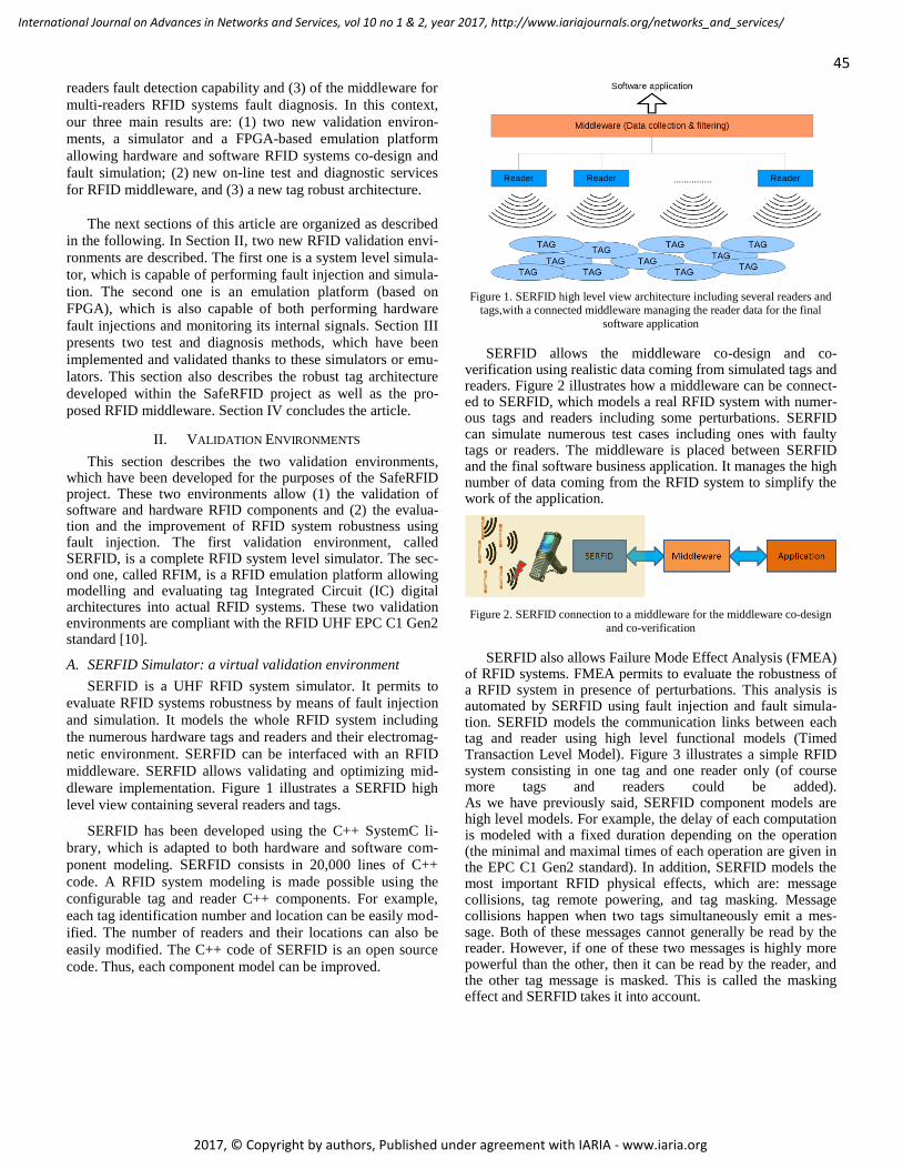
readers fault detection capability and (3) of the middleware for
multi-readers RFID systems fault diagnosis. In this context,
our three main results are: (1) two new validation environ-
ments, a simulator and a FPGA-based emulation platform
allowing hardware and software RFID systems co-design and
fault simulation; (2) new on-line test and diagnostic services
for RFID middleware, and (3) a new tag robust architecture.
The next sections of this article are organized as described
in the following. In Section II, two new RFID validation envi-
ronments are described. The first one is a system level simula-
tor, which is capable of performing fault injection and simula-
tion. The second one is an emulation platform (based on
FPGA), which is also capable of both performing hardware
fault injections and monitoring its internal signals. Section III
presents two test and diagnosis methods, which have been
implemented and validated thanks to these simulators or emu-
lators. This section also describes the robust tag architecture
developed within the SafeRFID project as well as the pro-
posed RFID middleware. Section IV concludes the article.
II. VALIDATION ENVIRONMENTS
This section describes the two validation environments, which have been developed for the purposes of the SafeRFID project. These two environments allow (1) the validation of software and hardware RFID components and (2) the evalua-tion and the improvement of RFID system robustness using fault injection. The first validation environment, called SERFID, is a complete RFID system level simulator. The sec-ond one, called RFIM, is a RFID emulation platform allowing modelling and evaluating tag Integrated Circuit (IC) digital architectures into actual RFID systems. These two validation environments are compliant with the RFID UHF EPC C1 Gen2 standard [10].
A. SERFID Simulator: a virtual validation environment
SERFID is a UHF RFID system simulator. It permits to
evaluate RFID systems robustness by means of fault injection
and simulation. It models the whole RFID system including
the numerous hardware tags and readers and their electromag-
netic environment. SERFID can be interfaced with an RFID
middleware. SERFID allows validating and optimizing mid-
dleware implementation. Figure 1 illustrates a SERFID high
level view containing several readers and tags.
SERFID has been developed using the C++ SystemC li-
brary, which is adapted to both hardware and software com-
ponent modeling. SERFID consists in 20,000 lines of C++
code. A RFID system modeling is made possible using the
configurable tag and reader C++ components. For example,
each tag identification number and location can be easily mod-
ified. The number of readers and their locations can also be
easily modified. The C++ code of SERFID is an open source
code. Thus, each component model can be improved.
Figure 1. SERFID high level view architecture including several readers and tags,with a connected middleware managing the reader data for the final
software application
SERFID allows the middleware co-design and co-verification using realistic data coming from simulated tags and readers. Figure 2 illustrates how a middleware can be connect-ed to SERFID, which models a real RFID system with numer-ous tags and readers including some perturbations. SERFID can simulate numerous test cases including ones with faulty tags or readers. The middleware is placed between SERFID and the final software business application. It manages the high number of data coming from the RFID system to simplify the work of the application.
Figure 2. SERFID connection to a middleware for the middleware co-design
and co-verification
SERFID also allows Failure Mode Effect Analysis (FMEA) of RFID systems. FMEA permits to evaluate the robustness of a RFID system in presence of perturbations. This analysis is automated by SERFID using fault injection and fault simula-tion. SERFID models the communication links between each tag and reader using high level functional models (Timed Transaction Level Model). Figure 3 illustrates a simple RFID system consisting in one tag and one reader only (of course more tags and readers could be added). As we have previously said, SERFID component models are high level models. For example, the delay of each computation is modeled with a fixed duration depending on the operation (the minimal and maximal times of each operation are given in the EPC C1 Gen2 standard). In addition, SERFID models the most important RFID physical effects, which are: message collisions, tag remote powering, and tag masking. Message collisions happen when two tags simultaneously emit a mes-sage. Both of these messages cannot generally be read by the reader. However, if one of these two messages is highly more powerful than the other, then it can be read by the reader, and the other tag message is masked. This is called the masking effect and SERFID takes it into account.
45
International Journal on Advances in Networks and Services, vol 10 no 1 & 2, year 2017, http://www.iariajournals.org/networks_and_services/
2017, © Copyright by authors, Published under agreement with IARIA - www.iaria.org

Figure 3. SERFID architecture of a simple RFID system including one tag, one reader, one channel and a global environment for the storage of global parameters
The power of each message depends only on the tag to reader distance and is computed with the Friss transmission equation. The remote powering modeling consists of adding all electromagnetic power emitted by all readers depending on their distance to the tags. The fault injection and simulation functionalities consider three different fault models: channel inactivation, no communication, and Bit-Error-Rate (BER) variation. Channel inactivation means that no power and no information are exchanged into a given channel during a spe-cific period. No communication model means that no infor-mation is exchanged into a given channel during a specific period (but power is still emitted). BER involves the injection of error in the exchanged bits. These bit error injections can be done with different random models (uniform, burst, etc).
In order to illustrate the use of SERFID, we describe in the following a real case study. This case study is inspired from a classical RFID application in a warehouse context. In this con-text, the goal of the RFID system is to identify the boxes (more than 100 boxes) arranged within a pallet. As illustrated in Fig-ure 4, this pallet is rotating between two RFID reader antennas. This environment is highly disturbed due to the numerous reflections of the electromagnetic waves on the products into the boxes. The rotation of the pallet helps for the tag detections.
This harsh environment requires the use of a robust inven-tory approach in order to detect all the tags in a limited amount of time. Optimizing the parameters of this robust inventory can be done with SERFID.
In Figure 5, we compare the inventory results achieved by a real RFID system with the inventory results obtained with the SERFID simulation. Of course the two inventory read rate curves are not exactly the same. Indeed, an accurate modeling of a so complex electromagnetic environment is not possible (or would be very time consuming). However, the shapes of the two inventory read rate curves are nearly the same and the inventory duration estimation is quite good (160s in the real system versus 176s in the simulated one). The SERFID model is enough accurate to allow optimizing the inventory parame-ters and all the middleware design parameters.
Figure 4. Example of the inventory of boxes under a rotating pallet thanks to an UHF RFID system
46
International Journal on Advances in Networks and Services, vol 10 no 1 & 2, year 2017, http://www.iariajournals.org/networks_and_services/
2017, © Copyright by authors, Published under agreement with IARIA - www.iaria.org

Figure 5. Real RFID system inventory read rate curve (top) vs. SERFID
simulated inventory read rate curve (bottom)
More details on this simulator are given in [11].
B. RFIM: an emulation platform
The digital baseband of the tag itself is a very important
element concerning the safety and security chain for the whole
RFID system. It imports then to study the tag itself in order to
(1) explore its best architecture compliant with the standard in
terms of safety and security and (2) to analyze the effect of a
faulty tag on the rest of the system. A deep study of different
digital baseband architectures considering all the possible
interactions with the complete RFID system is not a trivial
task due to the complexity and the heterogeneity of this sys-
tem. Nevertheless, the validation of the tag itself should be
done considering all the interactions of the tag and the RFID
system. While digital design requires cycle accurate simula-
tion it becomes unpractical for large systems involving hard-
ware and software levels and a multitude of devices. Also, it is
necessary to provide IC designer a tool which allows a quick
validation of the circuit under design in order to avoid costly
design respins. It has then been decided to develop a hardware
emulation platform dedicated to RFID transponder dependa-
bility and security study.
Emulation permits to evaluate the UHF RFID tag within its
real environment considering interferences between tags
themselves and interaction with the upper layer of the system
from reader to middleware. Indeed, a minor tag modification
can have multiple incidences on system parameters such as
inventory time or other. Moreover the emulator is very flexi-
ble to explore different digital architectures while ensuring
compliance with the UHF standard. As depicted in Figure 6
below, the RFID emulator can be used within an RFID envi-
ronment including reader and other transponders or even other
emulators. This way, the emulator is placed within a real
RFID environment which allows accurately analyzing many
hard to simulate system effects.
Figure 6. Emulation based digital baseband validation
Thanks to the in-system validation capabilities inherent to
the emulation, the proposed platform offers many opportuni-
ties. The emulation platform has been enhanced in order to be
able to monitor and to control in real time internal states of the
digital baseband. It is thus possible to perform fault injection
within the digital baseband. Emulation allows bit level fault
injection such as single event upset (SEU) or multi event upset
(MEU). It has been experimentally shown in [12] that this
fault model is realistic with the failure types of RFID tag IC.
While in-system validation allows identifying the most critical
faults from a system point of view, observing capabilities
helps to understand fault propagation in order to finely tune
mitigation techniques reducing the cost of the hardening. The
emulation based platform which has been developed is depict-
ed in Figure 7. This platform embeds a digital baseband fully
compliant with the UHF EPC C1 Gen2 protocol. As shown in
Figure 7, the RFIM platform is divided into eight modules:
monitoring interface, fault injector, activation of injection,
event detector, golden and instrumented faulty tags, register
comparator and embedded microprocessor. The embedded
microprocessor controls all the platform modules and then
permits to perform on-line tag monitoring and to play on-line
fault attacks. The processor allows the on-line capture of data
in the two tag basebands for analyzing the RFID communica-
tion. The interface monitoring is a mechanism that transports
the internal register values from the tag basebands to the mi-
croprocessor. This monitoring interface block uses a First-In-
First-Out (FIFO) memory in order to compensate the latency
of the microprocessor for outputting register values. Faults are
only injected in the faulty tag. The golden tag, which is always
fault free served as a reference. The register comparator com-
pares all the internal registers of the golden and the faulty tags.
This comparison helps the embedded processor to detect and
to localize faults and errors in the faulty tags.
RFIM allows quick and accurate validation taking into ac-
count all the complex physical effects involved into RFID
systems. Also, RFIM can be used in order to tackle security
issues of RFID systems.
47
International Journal on Advances in Networks and Services, vol 10 no 1 & 2, year 2017, http://www.iariajournals.org/networks_and_services/
2017, © Copyright by authors, Published under agreement with IARIA - www.iaria.org

Fault injector
Embedded Microprocessor
Activation of injection
Event detector Golden tag
Reg Comparator
Faulty tag
Monitoring interface
Figure 7. RFIM platform for faults injection and monitoring
First the emulator can be configured to process attacks
coming from the tag against the RFID system. Then system
level countermeasure can be developed and validated against
real case attacks. As an example, RFIM can be used to evalu-
ate the Hardware Trojan (HT) threats against RFID system
and to validate appropriate system countermeasure. HT threats
are malicious modifications of the circuit (such as backdoor)
which can later be used when the circuit is in mission mode.
RFIM allows then to emulate HT to attack the RFID system
using off the shelf reader and middleware in order to identify
weakest points which can be further secure. Moreover, the
EPC protocol offers room for cryptographic based security.
Nevertheless, one main limitation of such security is the in-
herent cost in time. So, using the emulator, cryptographic add-
on of the EPC protocol can be validated considering the whole
chain and then finely evaluate the associated cost such as the
time overhead for a given inventory.
III. TEST AND DIAGNOSIS METHODS AND TAG ROBUSTNESS
ENHANCEMENT
This section describes the three main approaches which have been proposed by the SafeRFID project in order to im-prove UHF RFID system dependability. Each approach is embedded on a specific part of the RFID system: the reader, the middleware and the tag digital architecture. These ap-proaches have been validated by simulation or emulation using the two previously described platforms and validated by exper-imentations.
A. Profile test method
The Profile test (PT) method is inspired by classical moni-toring techniques (ATTV, RETR), which are based on reader performance monitoring. This method, as the classical monitor-ing methods are, is nonintrusive. In this method, we propose to measure and compare individual tag performance indicators rather than a single global average parameter. To this end, we define a new performance metric - called read rate profile – individually involving all the tags of the population rather than an average value computed for the same population.
The initialization of our monitoring method requires com-
puting the statistical parameters of the fault free inventory read
rate profiles. Let us first explain what these inventory read rate
profiles are. Each tag inventory leads to a specific inventory
read rate profile, which is the ordered read rate curve of the
entire tag population. The ‘-‘curve in Figure 8 represents the
inventory profile of a fault free inventory occurrence. Then,
with numerous inventory profiles, an average read rate profile
is computed. This average profile is represented by the bold
curve in Figure 8.
The second step for the initialization of our approach con-
sists in computing a threshold for the failure detection. This
threshold, called limit profile, is represented by the ‘+’curve in
Figure 8.
Figure 8. Average, limit, fault free and faulty inventory profiles
0
10
20
30
40
50
60
70
80
90
100
1 11 21 31 41 51 61 71 81 91 101 111
Re
ad
Ra
te (
%)
Tag Index
Fault free profile
Faulty profile
Average profile
Limit profile
48
International Journal on Advances in Networks and Services, vol 10 no 1 & 2, year 2017, http://www.iariajournals.org/networks_and_services/
2017, © Copyright by authors, Published under agreement with IARIA - www.iaria.org

An inventory profile with one or more tag read rates under this limit implies that the RFID system is considered faulty. The ‘•’curve in Figure 8 illustrates a faulty inventory profile with several points under the limit. The limit profile is comput-ed using the average profile and the standard deviation of each ordered tags. The evaluation of this approach has been realized experimentally and by simulation. In both cases the detection results have been compared with the detection results of the RETR and ATTV classical approaches (described in the intro-duction).
1) Experimental validation. It is highly difficult to validate
the PT approach on real RFID systems. Indeed, it’s not trivial
to control the fault injection into these real systems and in
particular to be sure that each fault has been correclty injected.
Thus, we only did this experimental validation on a few
different scenarios. We use the same RFID application than
the one previously described in Section II.A. Some faults are
injected in this application to generate system faulty
behaviors. These faults are injected in the communication
channel only (no fault has been injected into the tag or the
reader hardware nor into the software components). The 3
different fault injection techniques are: - The rotation of 5 random tags on 5 different boxes - The displacement of 5, 15, and 20 random tags on the
surface of the boxes - The pallet rotation stop during 15s and 20s Using these fault injection techniques, a total of 9 faulty
system behaviors are generated. The RETR approach does not detect these faulty system behaviors. The ATTV approach detects 3 faulty system behaviors over the 9 faulty behaviors. The PT approach detects 4 faulty behaviors, and among these 4 faulty behaviors 3 were not detected by the previous approach-es. By conjointly using the PT and the ATTV approaches, it is then possible to detect 6 faulty behaviors over the 9 possible faulty behaviors. Finally the PT approach detects more faults than the classical approaches but this approach must be used with classical approaches to detect the maximum number of faults.
2) Evaluation with SERFID simulation. More scenarios
can be evaluated thanks to SERFID simulation. In the
following this evaluation is done using the 2 simple following
fault models: - 40% Read Rate decrease of 5 random tags - 10% Read Rate decrease of 20 random tags Each of these faults are injected and simulated 100 times to
obtain statistical representative results. Table I gives the detec-tion results achieved by the classical approaches and by the PT approach.
TABLE I. EVALUATION OF CLASSICAL ON-LINE TEST APPROACHES AND OF
PROFILE TEST (PT) APPROACH BY SERFID SIMULATION
5 random faulty tags
with Read Rate de-
creased of 40%
5 random faulty tags
with Read Rate de-
creased of 10%
ATTV 35% 11%
RETR 4% 5%
PT 63% 92%
Table I shows that the PT approach detects more faults than the classical approaches ATTV and RETR. As in the experi-mental validation achieved on an actual system, SERFID simu-lation of the ATTV approach shows that more faults are detect-ed than with the RETR approach. Once again the results show that the RETR and PT approaches are two complementary approaches. They have to be combined to achieve the best fault detection. In addition, the read rates of the tags which are im-pacted by the fault injection impact the performance of the PT approach. If the impacted tags have high read rates then the modification of the profile curve is more important than if the impacted tags have low read rates. Both Figures 9 and 10 show how the read rate values of the impacted tags modify the pro-file curve. In Figure 9 the impacted read rates have high values (the lowest one is 60%), and the fault injection drives to modi-fy the profile curve to achieve a fault detection (at 2 different locations corresponding to the 2 red circles).
Figure 9. Simulation of the profile curve modifications when faulty tags have
high read rates; the fault injection is detected at two different locations (two red circles)
Then, the next figure shows the case when the impacted read rates have low values. In this case the profile curve is not highly modified and no detection is achieved.
49
International Journal on Advances in Networks and Services, vol 10 no 1 & 2, year 2017, http://www.iariajournals.org/networks_and_services/
2017, © Copyright by authors, Published under agreement with IARIA - www.iaria.org

Figure 10. Simulation of the profile curve modification when faulty tags have
low read rates; no detection of the fault injection
Details on this test approach are given in [13][14] [15].
B. SafeRFID-MW: a Middleware for On-Line Testing and
Diagnosis
The proposed PT approach, as well as most existing test approaches (RETR, ATTV, etc.), operate mainly at the reader level. Obtained local results are not capitalized for global pro-cessing of errors at the whole system level. Consequently, in case of distributed RFID systems involving several readers, there are no means to determine the whole system state. Fur-thermore, in case of a faulty behavior, it is not easy to locate the origin of the observed failure: does it originate from the readers, the groups of read tags or the communications in-volved in the system?
In our work, this issue has been tackled by developing a dedicated RFID middleware that integrates not only testing operations at the level of each reader, but also a diagnosis pro-cess at the middleware level. By positioning this part of our study of RFID systems at the middleware level, the simultane-ous observations of many reading results are made possible. Consequently, analysis of these results can help producing a sharpened diagnosis and more accurately locate the likely causes of a failure. To this end, we applied the comparison of inventory results of several readers as it is done in the RF2ID middleware [8]. However, in our approach, comparisons are carried out among physical readers that read the same tag groups, providing inherent redundancy.
The random nature of the tag-reader interaction has di-rected our research towards the probabilistic diagnosis ap-proach [16] whose basic idea is to associate a probability of failure to each element in the system as well as a fault cover-age for each performed test. The user can then put a justified confidence in the obtained system diagnosis results. Our mid-dleware called SafeRFID-MW implements a diagnosis algo-rithm called RFID_Diag_Algo. This algorithm uses the basic idea of probabilistic diagnosis developed in the work of Fussel and Rangarajan on multiprocessor systems [16]. Nevertheless, the fault models, as well as the diagnosis operations, have been largely adapted to the RFID features. As a result, the diagnosis process we developed, takes place in two main phases. The
first phase consists of running the RFID_Diag_Algo algorithm. This one performs its operations in three steps: i) reader parti-tioning in groups according to some criteria issued by the ap-plication (i.e., which readers, read the same groups of tags), ii) read rate results comparison in a way that ensures a consen-sus on faulty components, whether readers or tags, iii) evalua-tion of the diagnosis accuracy by applying a new probabilistic model suitable to such systems. The second phase is executed for each identified faulty reader. It is based on the analysis of the communication logs between the faulty readers and the middleware to identify the precise cause of the observed fail-ure. Such information is not provided by the LLRP protocol and is therefore an innovative aspect of our work. The rest of this section provides more details on these two phases.
1) Description of the first phase (RFID_Diag_Algo): global probabilistic diagnosis. During this phase, RFID readers are partitioned into groups according to the actual paths of the tags through the various readers of the system. Thus, obtained groups include readers that process the same groups of tags (see Figure 11). For the example of Figure 11, we can observe that tags belonging to groups g1 and g2 are read by readers in the set (R1, R2, R3, R4, R5) whereas tags in the group g3 are read by readers in the set (R1, R2, R3, R4, R6, R7).
Figure. 11. Grouping of readers according to the data flow
Once tag groups are read by the corresponding readers, the
diagnosis process can start. At this point, our algorithm
RFID_Diag_Algo applies one of the aforementioned monitor-
ing approaches. This could be ATTV, RETR or the PT ap-
proach. The exact applied monitoring approach is not of im-
portance here, as only the obtained monitoring results matter.
Table II shows different inventories collected for a set of read-
ers (R1, R2, ..., R7) and 3 groups of tags g1, g2 and g3. The
value "1" indicates that the reader has ensured a correct inven-
tory of all tags while the value "0" indicates a failure of that
inventory. When a reader is not concerned by a group of tags,
the corresponding value is the "-" symbol.
The analysis of these results is done by applying the prin-
ciple of majority voting in the following two cases, using a
performance parameter that denotes the accuracy of each
reader results and whose calculation is presented in [17][18]:
50
International Journal on Advances in Networks and Services, vol 10 no 1 & 2, year 2017, http://www.iariajournals.org/networks_and_services/
2017, © Copyright by authors, Published under agreement with IARIA - www.iaria.org

1. If the majority of readers meet the considered performance
parameter, then the rest of the readers (i.e., the minority) are
considered faulty; i.e., the minority that shows poor perfor-
mance is considered faulty.
2. If the majority of readers do not meet the performance pa-
rameter set for the given group of tags, so this group of tags,
as well as the other readers, are considered faulty.
TABLE II. COMPARISON OF TAG INVENTORY RESULTS
Tag groups
g1 g2 g3
RFID readers
R1 1 0 1
R2 0 1 1
R3 1 0 1
R4 1 0 1
R5 1 0 -
R6 - - 1
R7 - - 0
R(gi) {R2} {R2, g2} {R7}
By applying this analysis, we obtain, for each group of tags
gi, a set of likely faulty readers and/or tags, as shown on the
row labelled R(gi) on Table II.
This phase of probabilistic diagnosis ends up with the de-
termination of a confidence parameter corresponding to the
quality of the diagnosis and hence, the trust level that the user
can have. At this stage, it is necessary to ensure the following
two points:
- A valid reader must be identified as valid (this case is
called "correct negative" and noted CN).
- A faulty reader must be identified as failing. To sim-
plify probabilistic calculations, we consider the com-
plementary case, that is to say the case where a faulty
reader is considered correct (this case is called a
"false negative" and noted FN)
We define the identifiability as being the probability of
correctly identifying the state of diagnosed readers. This
measure indicates the ability of the diagnosis process to "dis-
tinguish" the faulty readers from those who are not. This prob-
ability is the diagnosis accuracy and its calculation is detailed
in [15][16]. To give a little insight within this process, let us
consider again the example of Table II. We may simply state
that reader R2 is determined twice as being faulty whereas
reader R7 is determined only once as being faulty. So, in the
process of minimizing fault positives, the objective of the
diagnosis calculation is to determine more precisely the prob-
ability of each reader of being actually faulty. This may lead
to consider that R7 is actually fault-free.
2) Description of the second phase: Diagnosis of a faulty reader. After faulty readers have been identified, an additional study allowed us to pinpoint the causes of the observed failures. To this end, we analyzed the communication between the middleware and the RFID readers based on the LLRP protocol. Although LLRP is a complete and complex communication protocol that allows notifying the communication errors between the middleware and the readers, it can neither detect reader failures that are due to some misconfigurations, nor determine the causes of an observed failure. Therefore, it is not suitable as is for use in applications where dependability demands are critical, especially since the tag-reader interface is very sensitive to external disturbances and thus features a very random behavior. Furthermore, the functioning of the LLRP protocol is flexible and provides a wide autonomy to the application to specify the inventory operations and access to tags. This can lead to configuration errors resulting in a faulty behavior of the readers (for example, the reader cannot identify all tags in its reading range, the reader does not find the correct information on the tags, etc.).
Our work on the LLRP protocol mainly allows overcoming
these limitations. The study of the LLRP protocol led to its
modeling as a finite state machine. Let G denotes the finite
state machine of the LLRP protocol. G=(S, I, O, , ); where
I, O and S are respectively a finite set of input symbols, a
finite set of output symbols and a finite set of states.
- : S×I S is the state transition function.
- : S×I O is the output function.
When an RFID reader or the middleware is in a state s
S and receives input i I it produces a specified output
o=(s, i) O and transits to a state s = (s, i) S. Details of
this FSM are provided in [17]. For design or configuration
mistakes, the faulty behavior is associated with an inconsistent
state of the reader or the middleware. Indeed, the entity (read-
er or middleware) that is in an inconsistent state does not cor-
rectly interpret the received data and then adopts an inappro-
priate behavior. To tackle this type of mistakes, we applied to
the finite state machine of the LLRP protocol standard tech-
niques of model-based testing. More precisely, we used the
distinguishing sequences approach (Distinguishing sequences)
[18]. The application of this technique allows to simply re-
trieving the state in which the system was at the time of the
failure occurrence [18]. However, this technique has some
limitations as we cannot determine a distinctive sequence to
all the states represented within the FSM.
We also analyzed failures that are due to the runtime envi-
ronment, such as: slow execution, no data capture, etc. Such
faults cannot be related directly to a system state, since they
are mainly due to the execution environment. Thus, it is not
possible to simply apply the above approach. We therefore
proposed an extension of the state machine to include the
causes of this category of failures in the diagnosis process in
the form of an extended LLRP model [19][20]. The extensions
made to the LLRP protocol to determine the exact or likely
51
International Journal on Advances in Networks and Services, vol 10 no 1 & 2, year 2017, http://www.iariajournals.org/networks_and_services/
2017, © Copyright by authors, Published under agreement with IARIA - www.iaria.org

causes of observed failures are, to the best of our knowledge,
new features to RFID middlewares.
C. Tag Robustness Enhancement
Thanks to RFIM, the most sensitive parts of the tag digital
baseband architecture have been identified through fault injec-
tion campaigns [21]. The fault injection campaigns consist in
measuring for a given time period the number of times the tag
is detected by a reader while faults are injected in a part under
analysis of the tag digital baseband. This experiment has also
been done when several tags are in front of the reader in order
to evaluate the faulty tag effects on other tags. The experi-
ments have been carried out on all the functional registers (i.e.,
the registers storing parameter values dedicated to the com-
munication between tag and reader) of the digital baseband in
order to identify the most sensitive ones. Experimental results
[22] show that only a few registers dramatically decrease the
system performance (i.e., the tag read rate). Figure 12 hereaf-
ter gives the influence of the fault injection on the number of
times the tag has been successfully identified. Light gray gives
the value in case no faults are injected; dark gray gives the
resulting number in case faults have been injected within the
parameters given in horizontal axis.
At a first glance, we can see that all parameters are not
equally sensitive. While some faulty parameter registers re-
duce the number of times the tag has been identified from
4500 to less than 500, other ones have a very limited influence
on the tag response. This can be explained by the role played
by the parameter during an inventory round, and the refresh-
ment rate of the value during the same round.
We have proposed in a first approach to use hardware re-
dundancy to decrease the fault effects. A Triple Modular Re-
dundancy (TMR) has been applied on the most sensitive regis-
ters identified thanks to the previous fault injection campaigns.
Since the tag digital baseband architecture is powered wire-
lessly and has a limited resource, the TMR was chosen to
protect the most sensitive registers only. Moreover such regis-
ters are very small, which makes the cost acceptable. As
shown in Figure 13, the TMR technique consists on the tripli-
cation of the target component to be protected. The three re-
sulting outputs from triplication are connected to a voter block
that compares the three received data and elects the data with
the majority.
Figure 13. Triple Modular Redundancy Protection
.
Figure 12. Successful Tag Identifications number (y axis) for the most sensitive protected (Safe) or unprotected (Faulty) registers (x axis)
52
International Journal on Advances in Networks and Services, vol 10 no 1 & 2, year 2017, http://www.iariajournals.org/networks_and_services/
2017, © Copyright by authors, Published under agreement with IARIA - www.iaria.org

If one of the three components fails or suffers a direct SEU
then the fault is masked. In Figure 13, the target component is
a specific register storing a sensitive parameter. This register
is protected only against direct SEU impacting it. All the faults
impacting the combinational block before this register will be
propagated.
TMR technique implies an area increase of the redundant
part of more than 200% due to the component triplication. It
also needs a voter that is implemented just with some OR and
AND gates for each bit of the triplicated component. We have
experimentally noted that the use of this TMR improves the
read rate in the presence of faults into sensitive registers. The
proposed protection only adds 30 flip-flops to the whole cir-
cuit. Although expensive, TMR is in this case an acceptable
method since thanks to the fault injection campaigns the most
sensitive elements have been identified in a real RFID context,
limiting the TMR use to only a few bits. The TMR can thus be
tuned in order to replicate only flip-flops, which have been
identified as the ones having the higher influence on the tag
read rate in case of errors. We have also proposed and validated a complementary
approach allowing fault detection and diagnosis. This approach consists in adding hardware checkers into the tag circuit. Some of these checkers are provided by the synthesizable assertions available in the Open Verification Library (OVL) and others are designed to monitor tag finite state machine transitions. The faults detected by the checkers are counted and saved within the tag memory. Then, a user can read this information through the RFID reader and thereafter acquire diagnosis information. This approach has been implemented and evaluated on RFIM. Details on these robust architectures are given in [22].
IV. CONCLUSION AND FUTURE WORK
The SafeRFID project addresses the dependability issues
in RFID systems. The proposed framework considers both
hardware and software components as well as analog and
digital aspects of RFID systems. Three main layers have been
identified: the hardware layer with tags and readers, the com-
munication layer and the software layer including the RFID
middleware. The main results of this work are: (1) the devel-
opment of a fault simulator (SERFID) and of an FPGA based
emulator (RFIM) that allows fault injection and test method
evaluations, (2) the design and implementation of a robust
LLRP-compliant RFID middleware prototype that provides
fault detection and diagnosis new services, and (3) the devel-
opment of a tag robust architecture with self-diagnosis capa-
bility. The main perspective of this work is to consider fault
attacks and security issues related to RFID Systems. This issue
is a major concern in the context of Internet of Thing deploy-
ment. Then we will use the two developed platforms SERFID
and RFIM to validate new secure tags and system architec-
tures. These tags and systems will embed security functions
and authentication protocols.
ACKNOWLEDGMENT
This work has been supported by the French National Re-
search Agency project “SafeRFID” [ANR 2010 JCJC 0305
01]
REFERENCES
[1] V. Beroulle, O. Aktouf, and D. Hély, “System-Level Simulation for the Dependability Improvement of UHF RFID Systems,” ICWMC 2016, The Twelfth International Conference on Wireless and Mobile Communications, November 13 - 17, 2016 - Barcelona, Spain.
[2] R. Shorey, A. L. Ananda, M. C. Chan, C.-C. Chu, and W. T. Ooi, Mobile, Wireless and Sensor Networks: Technology, Applications and Future Directions, Chapter “WinRFID – A middleware for the enablement of Radio Frequency Identification (RFID) based Applications,” B. S. Prabhu, X. Su, H. Ramamurthy, C.-C. Chu, and R. Gadh, John Wiley and Sons Inc., 2006.
[3] Sun Microsystems, Inc., "Sun Java™ System RFID Software 3.0 Administration Guide," February 2006.
[4] A. Sengupta and S. Z. Schiller, “FlexRFID: A design, development and deployment framework for RFID-based business applications,” in Information Systems Frontiers, Vol. 12, n° 5, pp. 551-562, November 2010.
[5] N. Ahmed, “Reliable Framework for Unreliable RFID Devices,” in 8th IEEE International Conference on Pervasive Computing and Communications Workshops (PERCOM Workshops), Mannheim, 2010.
[6] F. Thornton, “How to Cheat at Deploying and Securing RFID,” Syngress Publishing ©2007, ISBN 1597492302 9781597492300
[7] C. Angerer and R. Langwieser, “Flexible Evaluation of RFID System Parameters using Rapid Prototyping,” in IEEE International Conference on Digital Object Identifier: 10.1109/RFID.2009.4911188 Publication Year: 2009 , pp. 42 – 47.
[8] C. Floerkemeier and S. Sarma, “RFIDSim—A Physical and Logical Layer Simulation Engine for Passive RFID,“ in Automation Science and Engineering, IEEE Transactions on Volume: 6 , Issue: 1 Digital Object Identifier: 10.1109/TASE.2008.2007929 Publication Year: 2009 , pp. 33 – 43.
[9] C. E. Palazzi, A. Ceriali, and M. Dal Monte, “RFID Emulation in Rifidi Environment,” in Proc. of the International Symposium on Ubiquitous Computing (UCS'09), Beijing, China, August 2009.
[10] EPCglobal, EPC Radio Frequency Identity Protocols Classe-1 Generation-2 UHF RFID, Protocol for Communications at 860 MHz 960 MHz, version 1.2.0, 2008.
[11] G. Fritz, V. Beroulle, O. Aktouf, and D. Hély, “SystemC Modeling of RFID Systems for Robustness Analysis,” in 19th International Conference on Software, Telecommunications and Computer Networks IEEE SoftCOM 2011Split - Hvar - Dubrovnik, September 15 – 17, 2011, IEEE Catalog Number: CFP1187A-CDR; ISBN 978-953-290-027-9.
[12] M. Hutter, J-M. Schmidt, and T. Plos. 2008. “RFID and Its Vulnerability to Faults,” in Proceeding of the 10th International Workshop on Cryptographic Hardware and Embedded Systems (CHES '08).
[13] G. Fritz, V. Beroulle, O. Aktouf, M. D. Nguyen, and D. Hély, “RFID System On-line Testing Based on the Evaluation of the Tags Read-Error-Rate,” in Journal of Electronic Testing:
53
International Journal on Advances in Networks and Services, vol 10 no 1 & 2, year 2017, http://www.iariajournals.org/networks_and_services/
2017, © Copyright by authors, Published under agreement with IARIA - www.iaria.org

Volume 27, Issue 3 (2011), pp. 267-276, (DOI: 10.1007/s10836-010-5191-6).
[14] G. Fritz, B. Maaloul, V. Beroulle, O-. Aktouf, and D. Hély, “Read Rate Profile Monitoring for Defect Detection in RFID Systems,” in IEEE International Conference on RFID-Technologies and Applications (RFID-TA 2011), pp. 89-94, Sitges, Barcelona, Spain, on September 15-16, 2011, IEEE Catalog Number: CFP11RFT-CDR ; ISBN: 978-1-4577-0026-2.
[15] G. Fritz, V. Beroulle, . Aktouf, and D. Hély, “Evaluation of a new RFID System Performance Monitoring Approach,” in Design, Automation & Test in Europe, (DATE 2012), Interactive Presentation, Dresden, Gremany, 12-16 March 2012.
[16] D. Fussell and S. Rangarajan, “Probabilistic Diagnosis of Multiprocessor Systems with Arbitrary Connectivity,” in IEEE 19th International Symposium on Fault-Tolerant Computing, FTCS-19. Digest of Papers., Chicago, IL, pp. 560-565, 1989.
[17] R. Kheddam, O. Aktouf, and I. Parissis, “Saferfid-MW: Safe and Fault-Tolerant RFID Middleware,” in Journal of Communications Software and Systems (jcomms), Special Issue on RFID Technologies and Internet of Things, Vol. 9, n° 1, March 2013, pp. 57-73.
[18] R. Kheddam, O. Aktouf and I. Parissis, “On-line Monitoring and Diagnosis of RFID Readers and Tags,” in 20th IEEE International Conference on Software, Telecommunications and Computer Networks (softcom 2012), Split, Croatia, 11-13 September 2012, pp. 1-9.
[19] R. Kheddam, O. Aktouf and I. Parissis, “An Extended LLRP Model for RFID System Test and Diagnosis,” in 8th Workshop on Advances in Model Based Testing, Montreal, Canada, 17-21 April 2012, pp. 529-538.
[20] R. Kheddam, O. Aktouf, I. Parissis and S. Boughazi, “ Monitoring of RFID Failures Resulting from LLRP Misconfigurations,” in 21st IEEE International Conference on Software, Telecommunications and Computer Networks (softcom 2013), Split, Croatia, Septembrer 2013, pp. 1-6.
[21] O. Abdelmalek, D. Hély, and V. Beroulle “Fault Tolerance Evaluation of RFID Tags,” in IEEE Latin America Test Workshop (LATW 2014), Fortaleza, Brésil, 13-16 March 2014.
[22] O. Abdelmalek, D. Hély, and V. Beroulle “Emulation of Faults Injection on UHF Transponders,” in 17th IEEE Symposium on Design and Diagnosis of Electronic Circuit and System (DDECS 2014), Warsaw, Poland, 23-25 April 2014.
[23] I. Mezzah, O. Kermita, H. Chemali, O. Abdelmalek, D. Hély, and V. Beroulle, “Assertion based on-line fault detection applied on UHF RFID tag,” in 8th IEEE International Design & Test Symposium 2013, Maroc (2013).
54
International Journal on Advances in Networks and Services, vol 10 no 1 & 2, year 2017, http://www.iariajournals.org/networks_and_services/
2017, © Copyright by authors, Published under agreement with IARIA - www.iaria.org

www.iariajournals.org
International Journal On Advances in Intelligent Systems
issn: 1942-2679
International Journal On Advances in Internet Technology
issn: 1942-2652
International Journal On Advances in Life Sciences
issn: 1942-2660
International Journal On Advances in Networks and Services
issn: 1942-2644
International Journal On Advances in Security
issn: 1942-2636
International Journal On Advances in Software
issn: 1942-2628
International Journal On Advances in Systems and Measurements
issn: 1942-261x
International Journal On Advances in Telecommunications
issn: 1942-2601