the impact of foreign direct investment on the nigeria

European Scientific Journal November 2017 edition Vol.13, No.31 ISSN: 1857 – 7881 (Print) e - ISSN 1857- 7431

521

The Impact of Foreign Direct Investment on the

Nigeria Manufacturing Sector: A Time Series

Analysis

Rasaq Akonji Danmola

Adijat Olubukola Olateju Faculty of Social Sciences, Department of Economics,

Lagos State University, Ojo, Lagos, Nigeria

Abubakar Wambai Aminu Faculty of Social Sciences, Department of Economics,

Bayero University Kano, Kano State, Nigeria

Doi: 10.19044/esj.2017.v13n31p521 URL:http://dx.doi.org/10.19044/esj.2017.v13n31p521

Abstract

The objective of the study reveals that FDI in the Manufacturing

sector exacts a positive influence on the manufacturing output and the impact

is statistically significant. This result further confirms the effectiveness of

economic policy of the federal government of Nigeria through the adoption

of liberalized industrial and trade policies. These policies were undertaken

with a view to improve efficiency and productivity, as well as to improve the

competitiveness of the Nigerian manufacturing industry. The policy

implication is that,in order to maintain sustainable economic growth and

development, a positive domestic investment is a prerequisite for increasing

the flow of foreign investment in the manufacturing sector. Nigeria, while

continuing to encourage inward FDI, efforts should be made to channel it

into the manufacturing sector so as to accelerate the diversification process.

In addition, the implementation of policy of trade liberalization should be

reviewed and implemented with caution. The policy that will further make

the economy more-import dependent will not augur well for the economy.

Keywords: Foreign Direct Investment to Manufacturing sector (FDIm),

Manufacturing output, Variance Decomposition, Impulse Response function.

1.0 Introduction

The manufacturing sector has been one of the major contributors to

Nigeria’s economic growth, but unfortunately, after witnessing tremendous

growth between the mid-1970s and the1980s, the sector experienced serious

stagnation, and for most of the 1980s and the1990s, Nigeria’s productivity

http://dx.doi.org/10.19044/esj.2017.v13n31p521


522

declined. This serious problem can be attributed to the downward trend in

the global oil market and the consequent fall in oil prices.

Governmentrevenue, coupled with foreign exchange earnings,

weredrastically affected by the problems experienced in the oil market, and

the government was therefore forced to adopt a series of economic reform

policies such as austerity measures. This prevailing situation has negatively

affected the manufacturing sector. In addition to this, serious trade control

policies, like the rationing of foreign exchange, import restrictions via import

licensing and tariff hikes, as well as quantitative measures, were put in place.

The above trade controls and industrial policies have causeda serious

fall in foreign exchange allocation to this sector, and have led to a reduction

in the importation of industrial raw-materials and spare parts available for

production in the sector.Thecosts of importing these essential industrial

inputs were prohibitive, and the foreign exchange needed for

suchprocurement wasin short supply. The situation has resulted in

widespread industrial closures, massive job cuts and a massive drop in

capacity utilization. The sector recorded a fall in real output of40 percent

between 1994 and 1996 and, since then, the sector has continued to

experience a downward trend in real output. The capacity utilization of the

manufacturing sector has not moved above 80 percent at any time over the

past thirty years, as can be seen in Figure 1

10

20

30

40

50

60

70

80

1980 1985 1990 1995 2000 2005 2010

Average Capacity Utilisation

Source: Central Bank of Nigeria statistical Bulletin Various Series from 1980-2014

Figure 1: Average Capacity Utilization of Manufacturing Sector 1980-2014


523

From Figure 1 above, the average capacity utilization in the

manufacturing sector since 1984 has been less than 60 percent, and most

manufacturing firms have been operating below production capacity; this has

negatively affected the sector. This problem has made it difficult for firms to

meet local demand, let alone to produce for export. The sector was

confronted with a shortage of raw-material for production, and did not have

the necessary foreign exchange for the importation of spare parts needed for

production.

Apart from the above problems, the cost of doing business in the

sector is high. To achieve a reasonable growth in the manufacturing sector, it

has often been suggested that Nigeria, like other developing country, needs

to embark on the intensive mobilization of both domestic and foreign capital

in order to accelerate sustainable economic growth. However, a careful look

at Table 1 below clearly shows that the cost of doing business is very high.

Macroeconomic variables that are vital to the availability of financial

resourcesinthe manufacturing sector are considered in Table 1. The

macroeconomic variables considered include Gross Fixed Capital

Formation–GDP ratio (GFCF/GDP), Savings–GDP ratio (SAV/GDP),

Lending Rate (LR), and Credit to Private Sector–GDP ratio (CPS/GDP).

With this trend, meaningful investment could not be generated

domestically and a large proportion of income was spent on consumption.

The savings–GDP ratio reached 8.6 by 2002 and, by implication;a larger

percentage of GDP went onconsumption before this figurerose to 37.78 in

2010. The credit available to the private sector was not encouraging and the

ratio of the GDP fell to an all-time low of 12.8 in 1993.Equally, the issue of

the mobilization of savings in the Nigerian economy left much to be desired.

The savings–GDP ratio is abysmal and not encouraging.

Table 1 clearly shows that the Nigerian manufacturing sector is

confronted with the problem of financial resources, which are in short

supply. The ratio of gross fixed capital formation (that is, domestic

investment) to GDP, for instance, fell to 5.5 in 2005, before it rose

significantly in 2010 to 13.7. In the same vein, the lending rate is prohibitive

for any meaningful productive investment. Nigeria’s lending rate reached its

peak in 1993, when it was 36.09 percent (CBN, 2014). This lending rate does

notgive room for any productive investment to take place, but is only good

for the services sector, where quick rates of return are expected;it cannot

propel any meaningful development in the manufacturing sector.


524

Table 1: Nigeria's Selected Economic Indicators

Year

LR

GFCF/GDP SAV/GDP

CSP/GDP

2000

21.3

7.2

8.4

12.3

2001

23.4

7.2

10.3

15.2

2002

24.8

7.9

8.6

13

2003

20.7

10.2

7.7

13.8

2004

19.2

7.6

7

13.1

2005

16.9

5.5

9

13.3

2006

16.9

8.3

9.4

13.3

2007

15.5

9.4

13

25.3

2008

18.4

8.4

16.9

33.9

2009

17.6

12.2

23.2

38.9

2010

14.1

13.7

20.4

29

2011

21.8

14.6

19.5

30.1

2012

22.6

15.2

17.4

33.9

2013

23.9

16.1

18.5

35.2

2014

14.1

10.2

21.8

36.1

Source: Central Bank Statistical Bulletin of Various Issues from 2000-2014

In most developing countries, FDI can theoretically be employed to

quicken the pace of industrial development, including in the manufacturing

sector, by providing industry, capital infrastructure, employment,

international market access, revenue and technology (Ratha, 2000).

However, the disparity between the success and the failure of developing

countries in practice to maximize the domestic gains and minimize the

negative externalities of foreign investment extended the questions about the

globalization of investment beyond thetheoretical frontiers. More

particularly, the issue of how beneficial FDI is fordeveloping countries forms

the kernel of empirical controversy (Aitken &Harrisson, 1999; Akinlo, 2004;

De Mello, 1997; Haddad & Harrison, 1993; Lipsey&Sjoholm, 2004). In fact,

different issues have emerged over the years, and these have led to various

controversies in the post-war history of North-South relations includingthose

connected with the impact of FDI in the industrialization of developing

countries.

Nigeria, given her natural resource base and large market size,

qualifies as a major recipient of FDI in Africa, and indeed, is one of the top

three recipients of FDI in Africa, but the volume of FDI attracted so far has

been mediocre compared with the resource base and potential need (Asiedu,

2012). The macroeconomic environment in Nigeria has not been conducive

for the thriving of FDI, and no investor wants to invest in a place where he

will suffer capital loss, no matter how promising and profitable it appears.


525

The pattern of the FDI that does exist is often skewed towards the extractive

industries (that is, the petroleum sector), so that it has been suggestedthat the

differential rate of FDI inflow into Nigeria is because of natural resources,

although the size of the local market may also be a consideration (Morriset

2000; Asiedu, 2002). Unfortunately, the efforts bymost countries in Africa,

including Nigeria, to attract FDI to real sectors of the economy, such as the

industrial and agricultural sectors, have not been encouraging. This

development is disturbing and means there is little hope of economic growth

and development for these countries.

There are good reasons for paying more attention toFDI. First, FDI

can bring development capital without repayment commitments, and this is

clearly differentfrom loan finance. Second, FDI is notmerely capital: it is an

important and potent bundle of capital, contacts and managerial and

technological knowledge, with potential spillover benefits for the host

country’s firms. Third, unlike other forms of capital flow, FDI has proved to

be resilient during crises (Dadush, Dasgupta and Ratha, 2000; Lipsey 2001).

This was evident in the Latin American debt crisis of the 1980s, the Mexican

crisis of 1994-1995, and the Asian financial crisis of 1997-1998. These traits

have encouraged intense competition for FDI amongdeveloping and

transition economies. In spite of the tremendous benefits, the controversy

still rages as to whether or not FDI constitutes a ladder to development. In

the midst of these controversies the need arises to assess the impact of FDI

flows and theattendant technologies of FDI forNigeria’s manufacturing

sector.

More importantly, FDI has been widely recognized as factors

explaining economic growth. Past empirical studies (both cross-country and

country-specific) into howFDIaffects growth (Karbasiet al., 2005;

Kohpaiboon, 2004; Mansouri, 2005) and the FDI–growth nexus, promote

economic growth and, by extension, improve manufacturing sector

performance. Nevertheless, there are clear indications that the growth

enhancing effects of FDIinflows vary from country to country. This means

that there has been diverse and, sometimes, conflicting empirical evidence

fromboth cross-country and country-specific analysis of the FDI–growth

nexus.

The overall implications of the catalogue of problems identified

above for Nigeria’s manufacturing sector are unimaginable, unless

something urgent is done. The researcher will be looking at the role of FDI

in reversing this trend and channelling the sector towards economic growth

and development.


526

1.1 The Flows of Foreign Direct Investment and

Industrial Policy in the Nigerian Manufacturing Sector

This section intends to review the flows of foreign direct investment

into the Nigerian manufacturing sector and industrial policy in place at the

different periods and more importantly, to further examine the flow of

technological transfer into the sector and policies of the government in the

area of research and development. This sub-heading will also examine the

performance of the manufacturing sector with the inflowof foreign direct

investment; with the emergence of trade liberalization policy and

technological transfer in the Nigerian economy.

1.1.1 The Performance of Nigeria Manufacturing Sector since

Independence (1960)

The manufacturing sector remains one of the vital sectors that can be

employed to propel economic development in most of the developing

countries including Nigeria. It acts as a catalyst in the transformation of the

economic structure of countries, from simple, slow-growing and low value

activities to more productive activities (Okonjo-Iweala and Osafo-Kwaako,

2007). As an engine of growth, a boost in manufacturing production offers

prospect of economic growth, and with the availability of manufactured

products, the speed of development can be enhanced. However, the output of

the Nigerian manufacturing sector has been very sluggish over the years.

This is particularly revealed when comparison is made with other sectors of

the economy. Following this trend and structure associated with the Nigerian

manufacturing sector, its impact in solving problem of poverty most

especially is questioned. The Nigerian manufacturing sector has witnessed a

series of fluctuations and unstable kind of growth and this has reflected in its

share on Gross Domestic Product (GDP) and to the economy as shown in the

Table 2-1 below. The problems associated with the manufacturing sector

persisted, in spite of the efforts of the government in establishing the

National Economic Empowerment Development Strategy (NEEDS), which

emphasized the relevance of rising manufacturing sector performance. The

history of industrial development and manufacturing in Nigeria is a classic

illustration of a country’s neglect of her agricultural sector and how this has

denied many manufacturing firms and industries their primary source of raw

materials.

There was a substantial growth experienced in the economy between

the mid 70s and 80s; since then, the manufacturing sector has experienced a

tremendous stagnation in output and for most of the period, it declined and

the problems has become more pronounced since 1983. The problem in the

manufacturing sector could be attributed to the fall in the global demand for

oil output and its adverse effect on the price of oil. The fall in oil prices in


527

the international oil market brought a fall in government revenue and

consequently, foreign exchange earnings was badly affected forcing

government to institute serious austerity measures. The manufacturing sector

suffered from a precipitous reduction in rawmaterials and spare parts caused

by these measures and these problems were translated into widespread

industrial closures, massive retrenchment of the industrial work force and an

extensive drop in capacity utilization from 71.5 percent in 1980 to

40.3percent and 36.1percent in 1990 and 2000 respectively before it

appreciated in 2010 to 55.14percent (CBN bulletin, 2010). But it should be

noted that there was never a time when the sector achieve 100percent in the

capacity utilization; this has brought a serious set-back to the sector and

further worsened its contribution to the country’s total export, which fell

from 42.7percent in the 1970 to 5.1 percent in 2010.This can further be

explained with the table 2 below:

Table 2: Selected Indicators of Performance in the Nigerian Manufacturing Sector

Indicators

1970 1980 1990 2000 2010

Share in GDP

(%)

7.2 10.4 3.5 6.4 1.93

Share in total

exports (%) 42.7 36.4 12.6 10.7 5.1

Share in total

imports (%) 35.2 28.9 27.2 30.2 35.6

Capacity

Utilization (%) NA 71.5 40.3 43.5 55.16

Value of

Manufactured

Exports (Million in

Naira) 378.4 5162.21 13847.5 156642.3 564432.9

FDI Flows to the

Sector (%) 22.4 41.5 60.7 44.6 39.5

Source: Central Bank of Nigeria (Statistical Bulletin 2010)

The share of the manufacturing sector in GDP as shown in the Table

2-1 rose from about 10.4 percent in 1980 as against 7.2 percent recorded for

the sector in 1970, but fell to all time low of 5.1 percent in 2010. A number

of factors accounted for this abysmal poor performance of the sector, chief

among which could be traced to inadequate access to raw-materials and

spare parts because of chronic foreign exchange shortage, that are required

for importation of needed industrial inputs. The inadequate industrial inputs

drastically affected industrial capacity utilization in the sector. The above

illustration provided vital information in the manufacturing sector when the

Structural Adjustment Programme (SAP) was initiated in 1986. The

programme aimed at enhancing the performance of the sector, though a


528

restructuring process was geared towards reducing import dependence and

promoting manufacturing products for export. This was further appreciated

in terms of the contribution of the sector to the country’s total exports which

was increased from about US378.4 million in 1970 to US564.5Billion in

2010.

To raise productivity in the sector, the Nigerian government laid

much emphasis on manufacturing sector because it was envisaged that the

modernization of the sector required a deliberate and sustained application

and combination of sustainable technology management techniques and

efficient system of mass production of goods and services (Malik, Teal and

Baptist, 2006). Unfortunately, in spite of the recorded increase in the FDI

inflows into the sector, the performance of the sector leaves much to be

desired as general output, capacity utilization and sector contribution to GDP

are still comparatively low. Also, the absence of locally sourced inputs as

pointed by Adenikinju and Chete (2002) has resulted in low industrialization.

It is quite evident that Nigeria’s industrial performance has been

disappointed in the last decade as the total manufacturing value added and

exports have declined in relative terms (Alukoet al., 2004). The problems

associated with the sector created a situation where Nigeria is losing its

competitive edge and is becoming increasingly marginalized in the

international industrial science due to unpredictable government policies

resulting from dynamic inconsistency, macroeconomic instability, a

distorting business environment, lack of basic raw materials, most of which

are imported and weak industrial capabilities. Consequently, the trend in the

performance of the industrial production cannot but indicate the falling

productivity, which has serious implications for aggregate demand.

Presently, the Nigerian manufacturing sector is lagging behind other

sectors in terms of productivity. The year 2010 brought some optimism by

the growth recorded as shown in Table 2-1 above. The capacity utilization

showed a slight improvement from 54.7 percent in 2009 to 55 percent in

2010. This development has been attributed to some policy initiatives aimed

at improving the performance of some firms within the sub-sector. The

policy initiatives include among others; granting of license for importation of

quality raw materials for industrial use, provision of capital allowance,

incentives for incurring excess capital expenditure, granting of input loan by

the ministry of commerce and industry in collaboration with the Central

Bank of Nigeria and commercial banks, provision of 2-3years duty free

period for importation of machinery, equipment and spare parts during the

phases of plant building and commencement of production, removal of

restrictions on investments in system conversion by manufacturing firms

(CBN bulletin, 2010). The important point here is that significant changes

are yet to be recorded in the sector. This justifies the need for policy


529

realignment potentially to help in building up indigenous manufacturing

technological capacity in the country.

The introduction of Structural Adjustment Programme in 1986 and

the emergence of a democratic government in 1999 provided opportunities in

building a competitive economy through various policies such as the

deregulation of various sectors among which is the manufacturing sector.

This period witnessed greater Foreign Direct Investment inflows from the

unimpressive flows of 22.4 percent in 1970 to the unprecedented flows of

about 41.5 percent and 60.7 percent in 1980 and 1990 respectively, before

experiencing a drop in 2010 to 39.5 percent (Table 2-1). It should be noted

that another factor responsible for this remarkable flow in FDI to the sector,

apart from the open economic policy regime, was the fact that the legal

regime and its related institutions required for the creation of a market

economy and sustainable investment climate were the priority of the public

policy agenda of the new civilian regime.

1.1.2 The Nigerian Manufacturing Sector and Industrial Policies from

Independence to Structural Adjustment Period (1986)

With the independence of Nigeria in 1960, trade policies have passed

through various stages that have changed remarkably over time. The first

stage of Nigeria’s trade policies was characterized by the protectionist

policies at independence in order to encourage industrial development that

will be in line with the strategy of import substitution policy of that time.

The second stage of the trade policy witnessed the era of the oil boom

phenomenon occasioned by the attendant economic buoyancy and

prosperity. This remarkable economic success propelled a relatively low tax

trade policy regime of the 1970s. Lastly, the next stage witnessed a tough

trade policy in response to the external balance position. This period was

characterized by the massive economic downturn and balance of payment

straits. The trade policies have in general become more restrictive in posture

and this was evidenced by the compression of imports through qualitative

barriers. These stages will further be elaborated.

The emergence of the indigenization policy initiated in 1972 was

tagged “the Nigerian Enterprises Promotion Decree” (NEPD). The decree

imposed several restrictions on FDI entry into the manufacturing sector. As a

result, some 22 business activities were exclusively reserved for Nigerians,

including advertising, gaming, electronic manufacturing, basic

manufacturing etc. Foreign investment was permitted up to 60 percent

ownership and provided that the proposed enterprise based on 1972 data,

possesses share capital of US$300,000 or turnover of US$760,000.


530

The objectives of the Nigerian Enterprises Promotion Decree of 1977

(which is the second indigenization policy) include

• Transfer ownership and control to Nigerians in respect of those

enterprises formerly owned (wholly or partly) and controlled by

foreigners;

• Foster widespread ownership of enterprises among Nigerians

citizens;

• Create opportunities for Nigerian indigenous businessmen;

• Encourage foreign businessmen and investors to move from the

unsophisticated spheres of the economy to domains where large

investments are required.

The above decree tightened the restrictions on FDI entry in three ways:

(a) by expanding the list of activities exclusively reserved for Nigerian

investors such as bus services and film production, (b) by lowering permitted

foreign participation in the FDI-restricted activities from 60 percent to 40

percent which included some manufacturing firms like processing firms and

plastic and chemical manufacturing firms, (c) by creating a second list of

activities, where foreign investments were permitted, was reduced from 100

percent to 60 percent ownership, including manufacturing of drugs, some

metals, glass, hotels and oil services companies. A critical appraisal of the

industrial development challenge of the 1970s shows that the hindrance was

not located in the area of finance but in the dearth of human capital including

techno-managerial capabilities and skills required for initiating,

implementing and managing industrial projects (Oyelaran-Oyeyinka, 1997).

This was further demonstrated by the fact that project preparation, feasibility

studies, engineering drawings and designs including construction, erection

and commissioning were contracted to foreign expatriates (Cheteet al. 2013).

The challenges of the 1980s necessitated the implementation of

Structural Adjustment Programmes (SAPs) under the auspices of the World

Bank and International Monetary Fund. This was due to the worsening in the

balance of payment position of the country’s economy resulting in the oil

crisis, acute deterioration of the terms of trade and exacerbation of excess

demand for imports originating from deficit financing of public expenditure,

and an increase in public debts. The adjustment programme was aimed at

diversifying the economic base, ensuring appropriate price and incomes

policy, increasing efficiency, improving the policy environment for

manufacturing and trade and restructuring of fiscal budgetary and

expenditure (Chirwa and Zakeyo, 2003). The statistics in the table below

support the thinking that the manufacturing sector in Nigeria performed

relatively better during the import substitution and protectionist policy period

(that is, the period 1960 to 1982), than during and after implementation of

economic liberalization policies.


531

Table 3: Trade Policies and Manufacturing Performance at Different Periods

Period Import Substitution Industrialization Average

manufacturing

growth

1960-1982 • Overvalued Exchange rate System-

Fixed Peg

• Non-tariff barriers to trade e.g.

import licensingand implicit foreign

exchange rationing

17.1 percent

• Active government involvement in

manufacturing industries

• Low and Stable inflation and

interest rate

1983-1998 Structural Adjustment Period

Average

manufacturing growth

• liberalization into manufacturing

sector

-3.69 percent

• Bilateral trade agreements

• Elimination of quantitative trade

restriction and exchange rationing

• Privatisation of State-Owned

enterprises

• Introduction of Export processing

zones

• Liberalization of the financial sector

and interest rates

• Period devaluation of the local

currency andliberalization of

interest rates

1999-2014 Post-Structural Adjustment

/NEEDS Period

Average

manufacturing growth

• Promotion of local value-added and

diversifying exports

8.76 percent

• Imposition of high import tariffs on

finished goods

• Gradual Liberalization trade policy

regime

Source: Average manufacturing growth represent the Average manufacturing growth rate,

computed by authorized based on data from Central Bank of Nigeria statistical Bulletins

(Various Issues),extracted from the Central Bank of Nigeria Economic and Financial

Reviews (Various Issues).

1.1.3 Manufacturing Sector and Post Structural Adjustment

Programme Period

There was a significant shift in trade policy direction towards greater

liberalization as of 1986. This shift in policy direction was directly caused by

the adoption of the structural adjustment programme (SAP). The programme


532

was informed by the distortions in the economy, ushered in by the culture of

controls, made it necessary for the government to put in place urgent and

drastic steps to ameliorate the situation. Thus, in July 1986, the SAP was

introduced to tackle the problem of imbalances in the economy and efficient

allocation of resources. The main cardinal point of the programme includes;

i) Restructure and diversify the productive base of the economy in

order to reduce the dependence on the oil sector and on imports;

ii) Ensuring fiscal and balance of payments viability overtime;

iii) To ensure strong foundation for the sustainable, non-inflationary

growth; and

iv) Reducing the over-bearing influence of the unproductive

investments in the public sector, enhancing the sector’s efficiency

and consolidating the growth potential of the private sector.

A number of strategic plans were outlined to realize the broad objectives

of SAP. With respect to international trade, attention was directed to trade

liberalization and the pricing system, with emphasis on the use of

“appropriate price mechanism for the allocation of foreign exchange”. The

second-tier Foreign Exchange Market (SFEM) was then introduced, under

which the rate of the country’s domestic currency (Naira) was to be

determined through the market forces of demand and supply. The price

determination mechanism provided the means for ultimate allocation of

foreign exchange to the end-users against the erstwhile use of administrative

discretion. The application of import and export licensing became irrelevant

and consequently abolished. In addition, to encourage export under the

programme, the policy which required exporters to declare their export

proceeds to the Central Bank of Nigeria (CBN) was discarded. In effect,

exporters were encouraged to retain 100 percent of their export earnings in

their domiciliary accounts from which they could freely draw to meet their

eligible foreign exchange transactions.

The implementation of the policy over the years has not impacted

positively in the country’s manufacturing sector. Looking at the

manufacturing sector’s performance during this period, it shows that the

share of the manufacturing sector in the Gross Domestic Product (GDP has

been relatively low. In 1970, it was about 9 percent, in 1980, it was about 10

percent, in 1990, about 8 percent and 1998, it was about 6 percent and in

2008, it was 5.9 percent (CBN Annual Report). Even though in the 1990s,

particularly in 1994, manufacturing shares in GDP was about 7 percent, the

growth rate was a negative of about 8 percent. Also at that same period, the

overall manufacturing capacity utilization fell from over 70 percent in 1973

to 39 percent in 1986 and about 27 percent in 1998 (CBN Annual Report). It

should be noted that only when firms are efficient that their potential for

employment creation, enhancing technology adoption and ensuring equitable


533

distribution of economic opportunities and macroeconomic stability can be

attained (Inegbenebor, 1995).

1.1.4 Manufacturing Sector and the Policy of National Economic

Empowerment and Development Strategy (NEEDS) (From 1999

to 2014)

Nigeria’s trade and industrial policy regime as contained in the

NEEDS has been directed to raise the level of competitiveness of domestic

manufacturing firms, with a view to, inter alia, promoting local value-added

raw-materials and encouraging as well as diversifying exports. The policy

adopted under this programme was the gradual liberalization of trade regime.

Thus, the government intends to liberalize the trade regime in such a way

that the resultant domestic costs of adjustment do not outweigh the benefits.

This is the fundamental basis on which to gauge the direction and

implementation of the policy. To this end, the current reform packages are

therefore formulated in such a way that it allows a certain level of protection

of domestic industries. In concrete terms, the policy has translated into tariff

escalation, with high effective rates in several sectors and lower import

duties on raw-materials and intermediate goods that are not available locally.

In addition, the impositions of high import duties on finished goods were the

result of the policy perspective on the finished goods, which competed with

local production.

2.0 Literature and TheoreticalReviews of FDI

A critical review of the theories of FDI illustrates the basic

justification of cross-border investment. The existing literature suggests that

for the last thirty years, FDI emerged much more ambitious in scope. In the

1960s, the effect of exportation of FDI had been the major issue, as

evidenced by the Hymer-Kindleberger theory and Verom’s (1966) in the

product cycle theory. In the 1970s, however, the growth of the MNEs based

on a theory of transaction cost formed the principal emphasis. By the 1980s,

Dunning’s eclectic approach had gained prominence. In the 1990s, the host

country impact of FDI was subjected to empirical study and analysis.

2.1 The Neo-Classical Theory

Prior to 1960s, FDI and portfolio investment were considered as

portfolio investment. When capital started to move across national

boundaries, then capital movement came to be viewed separately from

portfolio investment. The source-firm had to contend with differences in

distance, time, markets, cultures, personnel, currency and host government,

which were usually favourable to the local competitors. The theory of FDI

had, therefore, to provide explanation why firms go against market elements


534

to carry-out business in foreign markets and nations. FDI was originally

believed to move from a country with low interest rate to those yielding

higher interest rates. This is however an inadequate explanation in justifying

investments across borders, since there had also been FDI transactions from

higher interest (rates) countries to those with lower interest rates.

In 1960s, Hymer caused a major breakthrough in the theory of FDI.

He came up with the industrial organisation perspective, which is often

referred to as oligopolistic theory. He emphasized that the movement of

capital in respect to FDI, is not associated with higher interest rates, but due

to the financing international operations. Hence, market structure and

competitive conditions are vital determinants of FDI flow. Firm-specific

advantages and the firm’s market position have been employed to provide

explanation for the reason why MNEs engage in cross-border investments.

These merits must be enough to outweigh the demerits confronted by the

MNEs in competing with local firms.

Hymer concludes by asserting that international production has

substantial negative impacts on the host economies, since it raises market

barriers, increases concentration, limit the ability of the government to exact

control over national economy, and may put at risk national productive and

innovative products on the world demand. This is not that Hymer’s theory

disregard location advantages, but rather he treats it as exogenous factor

related to the MNE’s behaviour. Hymer’s work spawned many other

contributors in the theory of industrial organisation. The industrial theory of

FDI was further extended by Caves (1971, 1974) and Kindleberger (1984).

In their studies, they deviate from perfect competition as the factors that

influences FDI, but placed more emphasis on the demerits of perfect

competition in terms of geographical and cultural differences that the MNEs

will face in their operation, when compared to domestic firms. For MNEs to

be successfully embarked on FDI in a foreign country, they are required to

possess some special ownership advantage over potential domestic

competitors. The acquisition of technological advantage normally gives them

some intangible rent yielding assets such as management skills and brands,

which they believed to provide such advantages. This situation clearly, can

be distinguished from portfolio management, which only includes cross-

border flow of capital. It becomes imperative to state that FDI involves

cross-border movement of different kind of resources in terms of product and

process technology, management skills, marketing, distribution of technical

skills, marketing distribution of technical skills and human capital. In clear

terms, FDI includes a movement of intangible assets such as technological

know-how across countries and inability to consider the technological skill

can further underestimate the significance of FDI as an engine of growth for

the recipient countries. But it should be noted that, the cost and benefits of


535

such foreign capital in term of spillover effects have been largely ignored by

the earliest theorists of FDI.

Another important theory so identified in literature in explaining the

costs incurred by MNEs in the choice of locations and motives for

international investment across national borders is the location theory

provided by Buckley (1985; 1990). The theory considered the supply (cost

factors) and demand (market factor) variables influencing the spatial

distribution of the production processes, research and development (R&D)

and the administrative functions of a firm. In respect to the host country, it

was generally believed that the host country must obviously have some

location-specific advantages such as lower wages, abundant raw materials,

investment incentives, tariff and non-tariff protection, free trade zones,

among others.

Furthermore, currency area has equally been introduced as an

important dimension of the theory of FDI, as developed by Aliber (1970;

1971). He rejects arguments based on superior managerial skill because any

of such superiority should take into account the costs and exchange rate. The

implication is that some currencies are stronger compared with others, and

firms operating in strong currency areas can compensate for the capital

deficiency in weak currency areas through their own borrowings. This

position was supported from the empirical observations that devaluation

promotes FDI flow.

2.2 The Internalisation Theory

The origin of this theory was established in literature by Coase

(1937) in his market failure, who argued that transaction costs on foreign

activities make it more conducive for a firm to create an internal market as

oppose to entering foreign markets. The idea has been further expanded by

Buckley and Casson (1976). The internalisation theory proposed by Buckley

and Casson (1976), investigate the choice between exporting and

establishing a subsidiary in a major export locations. Expansion by FDI can

be a viable alternative for a MNE, when it has an edge in term of competitive

advantage over other firms. This firm-specific advantage needs to be

safeguarded by the organisational structure, and by implication, it means that

FDI becomes favourable when the benefits of internalisation outweigh its

costs.

The impact of MNEs as an avenue for international diversification

has been analyzed by Rugman (1979), who extended the internalisation

theory and included FDI as a possible instrument. According to him, while

internalisation is helpful in bringing about internal markets, bypassing capital

market imperfection, it is also, at the core of the MNE concept, highly

consistent with the transaction cost and eclectic theories.


536

2.3 Product Life Cycle Theory

The major contributor to this theory was put forward by Vernon

(1966). Vernon’s (1966) study is anchored on the experience of the post-

second world war period and companies sequences involving domestic

versus foreign production. In his model, FDI has been regarded as replacing

trade. The product life cycle hypothesis states that based on the comparative

advantage emanating from the pattern of factor endowments, a product

invented in the home country initially enjoys competitive advantage in

technology and inventory capabilities and serves the local markets.

At the next stage, a favourable combination of innovation and

technological advantages makes the product an exportable commodity to

countries where conditions are very similar to the home country. As the

product gradually becomes standardized and labour becomes a significant

input in terms of production cost, a foreign country location may become

more attractive. The process could grow to such an extent that the home

country could in itself be a recipient. Vernon (1979) reviewed his theory and

opines that it had less power in elucidating the reasons for FDI. He combined

the geographical reach of many firms and emphasized on gap reduction

between the US and other national markets in respect to both size and factor

cost. Although, current development could perhaps make various stages of

product life cycle less applicable, it cannot be disputed that the theory

remained valid in explaining the rational process leading to FDI.

It needs to be emphasized at this junction that the product life cycle

theory has been subjected to various modifications, so that recent changes in

the FDI theory could be accommodated. Grosse and Kujawa, (1995) opines

that product life cycle is a dynamic view of investigating the rationale for

trade flows in the context of changing technology and multiple markets.

They allied with Vernon’s view that the export market, which forms the

nucleus for FDI is the third stage of the product’s life cycle, is important and

low cost advantage is the significant consideration at this stage of decision

making.

2.4 The Eclectic Approach

Dunning (1977; 1979; 1993 1997) developed the eclectic theory by

synthesizing the current theories of FDI to identify and analysis the

important factors influencing FDI. FDI location will therefore depend on

three sets of factors:

(i) Ownership (O): the “O” advantages include marketing skills and

R&D skills or production skills that enable firms to provide goods and

services more competitively in their countries and in other countries.

(ii) Location (L): this includes low-cost labour, incentives to production

on the part of the host government, natural resources, domestic market


537

potentials, and political stability. These are not easily transferable between

countries and could differ from the home country situation. Ownership

advantages tends to provide answer on why some firms, but not others go

abroad, and provide an explanation that a successful MNE possess some

firm-specific advantages which allows it to overcome the costs of operating

in a foreign country. An important idea is the fact that firms are in control of

collection of assets and that these assets can be employed in production at

different locations without reducing their effectiveness. Example includes

product development, managerial structures, patents and marketing skills, all

of which are encompassed by the catch-all term of Helpman (1984)

“headquater services”.

It should be noted that international trade theory has tended to take

ownership advantages for granted; rather, more attention has been devoted to

exploring alternative motives for MNEs to locate abroad. An important issue

that motivated much attention is the distinction between “horizontal” and

“vertical” FDI. Horizontal FDI occurs when a firm locates a plant abroad in

order to improve its market access to foreign consumers. In this case, a firm

tries to replicate its domestic production facilities at a foreign location. While

in the case of vertical FDI, FDI is not primarily or even necessarily aimed at

production for sale at foreign market, but rather seeks to avail itself of lower

production costs there since in almost all cases the parent firm retains its

headquarter in the home country, and the firm-specific or ownership

advantages can be seen as generating a flow of “headquarter services” to the

host-country plant, this explains why all FDI is vertical in nature.

(iii) International (I): the “O” and “L”must be complimented by

internalisation to overcome transaction costs, such as those pertaining to

transport, information, different taxes and tariffs (which differ among

countries), and other market imperfections. It should be noted that OLI does

not directly address one of the important issues that dominated economists

thinking about FDI, the distinction between horizontal and vertical motives

for locating production facilities in foreign countries nor does it address the

increasingly important distinction between Greenfield and M&A modes of

engaging in FDI. Nevertheless, it remains a helpful way of organising

thinking about one of the most significant features of the world economy.

2.5 Macroeconomic Theory

This theory could be considered as a milestone in the theory of FDI.

It was introduced by Kojima (1973; 1984). The theories earlier discussed

were predominantly designed for US firms investing abroad, differentiating

them from Japanese FDI. The latter are primarily trade oriented and in line

with dictates of the principle of comparative advantage. In contrast, US

activity was mainly an oligopolistic market structure. There was less


538

emphasizes on trade and activity was directed on firm-specific profit

orientation. Kojima’s approach predicted that export-oriented FDI occurred

in countries with a comparative advantage for the host country. Thus, when

exports grow FDI is characterized as welfare-improving and trade-creating.

Due to Kojima’s preference for Japanese style management, his approach

has been considered to be biased and inadequate. Dunning (1988), for

instance, pointed out that Kojima’s neo-classical framework was inadequate

in capturing the impact of firm-specific advantage in determining FDI flow.

He further argued that Kojima’s theory is grossly inadequate in explaining

modern trade; it could not, for instance, provide adequate reason for trade

flows, which are based less on the distribution of factor endowments, and

more on the need to exploit the economies of scale, product differentiation

and other manifestations of market failure (Dunning, 1993).

3.0 Empirical Reviews

Adejumo, (2013), in his the study investigates the relationship

between FDI and the value-added to the manufacturing sector in Nigeria.

The study employs the autoregressive lag distribution technique to examine

the relationship between foreign direct investments and manufacturing value

added, it was established that in the long run, FDI have a negative effect on

the manufacturing sub-sector in Nigeria. He however, argues that the

presence of multinationals in the host economy should be able to influence

the private investment on their economy. Besides, these investments should

be channeled to other sectors where comparative advantage exists, so as not

to erode the capability or the wherewithal of nationals. He concluded that

foreign private investment should complement the production efforts of the

labour force in the host country, in term of skills, technical know-how and

wages.

Alvarez (2003) the study analysis the panel data from more than 7000

firms in the manufacturing industry for the period 1990-1996 in Chile. He

observed that MNEs’ affiliates present much higher levels of productivity

than do local firms. He further argues that FDI does positively impact on the

level of productivity. Nevertheless, the effects seem to be small in

magnitude. The small effect of FDI on the manufacturing may be attributed

to the low number of foreign firms operating in the industry, suggesting that

a bigger number of foreign firms may be necessary to bring about significant

impact on local firms. He also emphasizes that most of FDI inflows have

been directed to the mining and services industries.

Oscar and Simon (1994) investigate the inflow of FDI into Spanish

economy during the period 1964 to 1989 and using autoregressive

distributive lag technique, the study established a long-run relationship

between FDI and GDP, inflation, trade barriers and capital stock.


539

In analyzing the macroeconomic impact of FDI on China for 1979-

1993, Sun (1996) found that FDI contributed positively to Chinese domestic

capital formation, industrial growth, exports and employment creation. With

the data limitation faced by the study, he pooled cross-section and time series

data at the provincial level and formulated a regression model to test the

hypothesis. Sun (1996), applied the Generalized Least Squares (GLS)

method and the study establish that FDI had significantly contributed to the

economic development of China. The impact of FDI was seen as the main

contribution it had to domestic capital formation, promotion of industrial

production, exports and the creation of new employment. Sun (1996) further

stated that FDI contributed to financial and physical capital development and

encourages local investment.

Ekanayake et al. (2003) demonstrate the relationship between output

level, inward FDI and export across the developed and developing countries

(Brazil, Canada, Chile, Mexico and U.S) from 1960 to 2001 by using the

granger causality test. The results of the research are not consistent across

these countries. Importantly, a two-way causal relationship between inward

FDI and exports is found in the U.S and Canada and the existence of a one-

way, moving from inward FDI to export is established in Brazil, Chile and

Mexico.

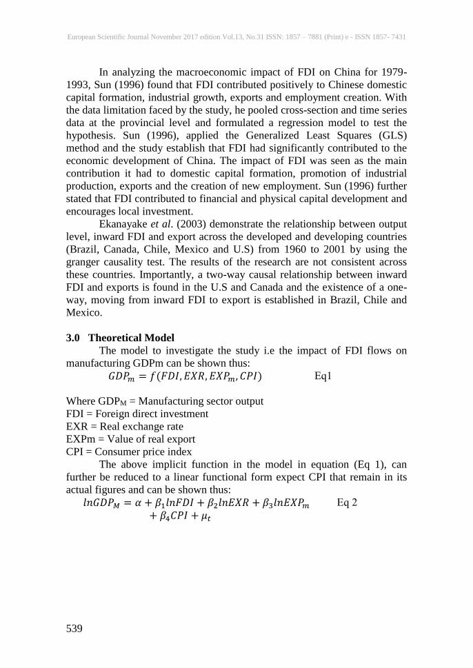
3.0 Theoretical Model

The model to investigate the study i.e the impact of FDI flows on

manufacturing GDPm can be shown thus:

𝐺𝐷𝑃𝑚 = 𝑓(𝐹𝐷𝐼, 𝐸𝑋𝑅, 𝐸𝑋𝑃𝑚, 𝐶𝑃𝐼) Eq1

Where GDPM = Manufacturing sector output

FDI = Foreign direct investment

EXR = Real exchange rate

EXPm = Value of real export

CPI = Consumer price index

The above implicit function in the model in equation (Eq 1), can

further be reduced to a linear functional form expect CPI that remain in its

actual figures and can be shown thus:

𝑙𝑛𝐺𝐷𝑃𝑀 = 𝛼 + 𝛽1𝑙𝑛𝐹𝐷𝐼 + 𝛽2𝑙𝑛𝐸𝑋𝑅 + 𝛽3𝑙𝑛𝐸𝑋𝑃𝑚

+ 𝛽4𝐶𝑃𝐼 + 𝜇𝑡

Eq 2


540

Apart from the linear regression that will be estimated above, the

study will further employed Variance decomposition and Impulse Response

functions in the analyses of the study.

3.1 Variance decomposition

Generally, VARs becomes over-parameterised with the inclusion of

many lags on the right-hand side of the equation, which makes short-run

forecasting difficult to achieve. To overcome this situation and understand

the relationship among the variables it is common to analyse the properties

of the of the forecast error. In order to gauge the relative strength of the

variables and transmission mechanism response, the system will be shocked

and partitioned the forecast error variance decompositions (FEVDs) for each

variable in the system. By partitioning, the variance decomposition

attributable to innovations in other variables in the system can provide an

indication of these relativities (Masih, 1995). The vector error correction

model does not provide any indication of the dynamic properties of the

system and also does not allow people to gauge the relative strength of the

Granger causality or degree of exogeneity among variables (Masih, 1995).

The variance decomposition analysis provides useful information

about the relative importance of each innovation in influencing the variables

in the system. This means that it is possible to separate the proportion of the

movements in a sequence due to its shocks and other variables’ shocks. We

can obtain the variance decomposition using the same Vector Moving

Average (VMA) representation that was previously obtained in Eq 3, if we

forecast yt+ƞƞ periods ahead, the ahead forecast error will be

yt+ƞ= µ + ∑∞𝒊=𝟎 𝜙i εt+ƞ-i

Eq 3

The ƞ-period forecast error is equal to the difference between the

realisation of yt+ƞand its conditional expectation:

yt+ƞ-𝐸(𝑦t+ƞ)=∑𝑛−1𝑖=0 ϕiεt+ƞ-i

Eq4

The variance of the n-step ahead forecast error, denoted as 𝜕yt(ƞ)2, for

each variable in the vector yt=(yit , y2t……yƞi) is equal to

𝜕yt (ƞ)2𝜕2yit (∑𝑛−1

𝑖=0 ϕi2) 𝜕2

y2t(∑𝑛−1𝑖=0 𝜙I

2) …..𝜕2yƞt(∑𝑛−1

𝑖=0 ϕi2)

Eq5

Fromthis expression it is possible to decompose the variance of the

forecast error and isolate the difficult shocks; particularly we can separate

the different proportion of the variance due to shocks in the sequence {εyt}.

For example, in the case of having only two variables, (yit and y2t ), the

variance decomposition of the forecast error ofyit can be found by dividing

equation Eq 5. In this way we can get the proportion of Ϭyt (ƞ)2due to

movements in its {εyit}and {εy2t}.


541

1=𝜕2 yit(ϕ11(0)2 ......ϕ11(ƞ-1)2+ 𝜕2

y2t {ϕ12(0).....ϕ12(ƞ-1)2 }

𝜕yit(ƞ)2 𝜕y2t(ƞ)2

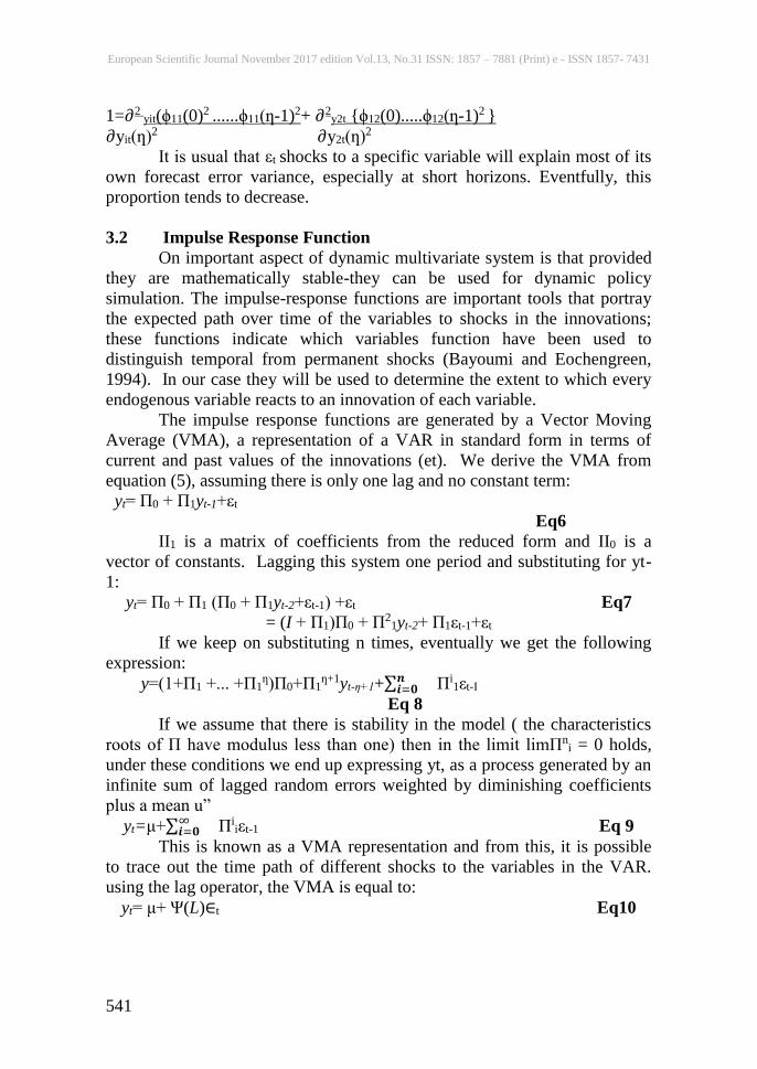
It is usual that εt shocks to a specific variable will explain most of its

own forecast error variance, especially at short horizons. Eventfully, this

proportion tends to decrease.

3.2 Impulse Response Function

On important aspect of dynamic multivariate system is that provided

they are mathematically stable-they can be used for dynamic policy

simulation. The impulse-response functions are important tools that portray

the expected path over time of the variables to shocks in the innovations;

these functions indicate which variables function have been used to

distinguish temporal from permanent shocks (Bayoumi and Eochengreen,

1994). In our case they will be used to determine the extent to which every

endogenous variable reacts to an innovation of each variable.

The impulse response functions are generated by a Vector Moving

Average (VMA), a representation of a VAR in standard form in terms of

current and past values of the innovations (et). We derive the VMA from

equation (5), assuming there is only one lag and no constant term:

yt= Π0 + Π1yt-1+εt

Eq6

II1 is a matrix of coefficients from the reduced form and II0 is a

vector of constants. Lagging this system one period and substituting for yt-

1:

yt= Π0 + Π1 (Π0 + Π1yt-2+εt-1) +εt Eq7

= (I + Π1)Π0 + Π21yt-2+ Π1εt-1+εt

If we keep on substituting n times, eventually we get the following

expression:

y=(1+Π1 +... +Π1ƞ)Π0+Π1

ƞ+1yt-ƞ+1+∑𝒏𝒊=𝟎 Πi

1εt-I

Eq 8

If we assume that there is stability in the model ( the characteristics

roots of Π have modulus less than one) then in the limit limΠni = 0 holds,

under these conditions we end up expressing yt, as a process generated by an

infinite sum of lagged random errors weighted by diminishing coefficients

plus a mean u”

yt=μ+∑∞𝒊=𝟎 Πi

iεt-1 Eq 9

This is known as a VMA representation and from this, it is possible

to trace out the time path of different shocks to the variables in the VAR.

using the lag operator, the VMA is equal to:

yt= μ+ Ψ(L)∈t Eq10


542

Matrix Ψ contains the impulse-response functions; a coefficient in Ψ

will describe the response of an endogenous variable yt at time t+s to a one

unit change in the innovation∈jt, ceteris paribus. Or:

∂yi,t,s

∂∈jt,

Eq11

s refers to the period. so we have that each coefficient measures the

response of the modeled series to shocks in the innovations. Depending on

the number of periods used in the equations, the impulse response functions

will show the time path due to shocks in the error terms. If the stability

condition is satisfied, the response of a variable to a shock in the system will

move it away from the its equilibrium but eventually will tend to return to it.

The speed of adjustment will depend of the influence of each shock in the

variable.

Unfortunately the residuals in the VAR are correlated and the model

is under identified; for this reason it is necessary to apply a transformation to

the innovation so that they become uncorrelated. One way is by transforming

the VAR in a model where the errors are not contemporaneously correlated;

this can be done through the orthogonalisation of the innovations (Charemza

and Deadman, 1997). Another way-which is used in this study, is the

Cholesky decomposition. This is a matrix decomposition of a symmetric

matrix into a lower triangular matrix and its transpose. In this case, using the

residual covariance matrix (Ὠ) as the symmetric matrix, we can decompose

it into”

Ὠ = PPT where P = AD1/2

Eq12

A is a lower triangular matrix with 1’s along the principal diagonal

and D is a unique diagonal matrix whose (j, j) element is the standard

deviation of the residual j. P is a lower triangular matrix. Using matrix A, we

can express vt as a vector of uncorrelated residuals vt=P-1∈t. The reason is

that D is a diagonal matrix that contains only uncorrelated elements. Every

column in P (denoted as pj) will capture how the forecast of all innovations

changes as a result of new information (besides the information contained in

the system). If we incorporate this component in (Eq 11) we get:

∂yt + s

∂yjt

Eq13

Each coefficient in the expression above will describe the response of

the endogenous variable to a unit change in the innovations over time.

Ψs

ΨsPj


543

4.0 Description and Sources of the Data

MFDI is the flow of foreign capital investment into the

manufacturing sector. The foreign capital can theoretically expedite the

process of industrial development as well as manufacturing sub-sector in

poor countries by providing industry, capital, infrastructure, employment,

international market access, revenue and technology (Lipsey, 2001; Ratha,

2005). The data is sourced from Central Bank of Nigeria.

GDPm is the value of the manufactured goods contributed to the

gross domestic product. The data is sourced from National Bureau of

Statistics.

CPI represents Consumer Price Index and it measures inflation in the

country and one of the classic symptoms of loss of fiscal or monetary control

is unbridled inflation (Nonnemberg and Mendoca, 2004). Therefore it is used

to capture the overall macroeconomic stability of the country and since

investors prefer to invest in more stable economies that reflect a lesser

degree of uncertainty. The data is sourced from UNCTAD statistical year

book published by United Nations on trade and development.

EXR represents Exchange rate and are expected to negatively affect

GDPm. This is so because they affect a firm’s cash flow, expected

profitability and consequently its contribution to the GDP of the

manufacturing sector. Exchange rate flunciations are as measure of

macroeconomic instability, the higher and more unstable it is, the less

contribution to GDPm (ErdalTatoglu, 2002; Maniam, 1998). The data for

nominal exchange rate are sourced from National Bureau of Statistics and

stated in real form.

Error term µ: the error term represents uncontrolled country specific

factors such as demand shocks, business cycle, labour market wages as well

as conflicts, international business situation as well as measurement error in

the dependent variable and omitted explanatory variables. The error term is

assumed to be independently and identically distributed.

EXPm represents manufacturing exports and this is the volume of

manufacturing exports and affects the GDPm positively. The export is

capable of reducing the country’s balance of payment disequilibrium. The

positive effect on GDPm is hypothesized. The data for manufacturing

exports are sourced from Central Bank of Nigeria Statistical Bulletin of

various issues up to 2013 edition.


544

5.0 Analysis and Results of the Study

Table 4: Ordinary Least Square

Duration: For the entire Period

Dependent Variable: LGDPm

Method: Least Square

Date: 09/20/15

Sample 19802013

Included Observation: 34

Variable

Coefficient Std.Error

t-statis

Prob.

C

9764.548

9584.22

1.01888

0.3167

LMFDI

0.87085

0.19852

4.38668

0.0001

LCPI

1306.306

214.037

6.10325

0

LEXR

-70.0714

130.639

-0.5365

0.5958

LEXPm

0.466698

0.12712

3.67156

0.001

R-Squared 0.987391

Mean Dependent Var. 208711.6

Adjusted R-

Squared 0.985652

S.D Dependent Var

241476.2

S.E of regression 28925.07

Akaike Inf. Criterion 23.51786

Sum Squared

resid 2.43E +10

Schwarz Inf. Criterion 23.74232

Log Likelihood -394.804

Hannan-Quinn

23.59441

F-Statistic 567.7317

Durbin Watson

1.101801

Prob. F-Statistic 0

VAR Granger Causality/Block Exogeneity Wald Tests (For the entire Period)

Dependent Variable

Δ(GDPm) Δ(CPI) Δ(EXPm) Δ(EXR) Δ(MFDI)

Δ(CPI) 37.7(0.00)*** - 5.74(0.06)* 0.35(0.553) 16.07(0.00)∗∗∗

Δ(EXPm) 13.84(0.00)*** 6.96(0.31) - 7.60(0.02)** 93.97(0.00)∗∗∗

Δ(EXR) 4.26(0.12) 1.97(0.37) 7.60(0.02)** - 0.103(0.748)

Δ(MFDI) 12.087(0.042)**

6.76(0.03)∗∗

0.18(0.076) 2.8(0.930) -

Δ(GDPm) -

8.29(0.02)∗∗

0.96(0.757) 0.18(0.670) 0.97(0.325)

The VAR result was based on 3 year lag structure and ∗∗∗,∗∗,∗ indicates statistically

significance at 1 percent, 5 percent and 10 percent levels respectively. Figures in parenthesis

() are P-value

In entire period, the regression result of the model shows that R-

Squared (Adjusted) is 98 percent, indicating that the co-efficient of


545

determination of the model of 98 percent of variation in the dependent

variable is explained by the independent variables in the model. More so, the

F-statistic of the model is 0.0000, which is quite significant at 1 percent

level. This implies that the model ascertain the overall significant of the

independent variables used in the model.

The regression of the model shows that LMFDI exact a positive

influence on the LGDPm and the influence is statistically significant. This

indicates that one percent rise in MFDI, will lead to 87 percent increase in

the GDPm. This tends to confirm the effectiveness of economic policy by

adopting a liberalized industrial and trade policy regime. The policy was

undertaken with a view to improve efficiency and productivity as well as to

improve the competitiveness of Nigerian industries. The policy makers in

Nigeria have undertaken series of measures in the past to attract foreign

investment to the manufacturing sector in the country. The result of the

measures put in place to attract investments into the sector in the past years,

confirm that foreign direct flows into the sector have increased in ten-fold.

But initially, the flows of the foreign investment were directed to petroleum

sector and this account for its insignificant performance to Manufacturing

Gross domestic product, but as the industrial and trade policies adopted by

the government take firm root, attentions are given to the manufacturing

sector in terms of flows of foreign direct investment.

Furthermore, the regression result also shows that exports of

manufactured goods exact positive influence on Manufacturing Gross

domestic product and it is even statistically significant in long run. This

result shows that one percent rise in EXPm will lead to 46.7 percent increase

in GDPm. This result confirms that the presence of MNEs with attendance

foreign capital inflow, this has altered the exports behavior of Nigerian

domestic firms in the area product and process innovation. This implies that

foreign direct investment into the sector have helped to improve local

manufacturing firms to produce goods not only to meet local market

demands but also to seek for the expansion in the export markets. This result

was confirmed in a study carried out by Rettab, Rao and Charif (2009),

where it was recognized with substantive evidence that a firm’s openness to

the external economy does positively affect innovative intensity. This can be

explained by the fact that expanding capacity to produce for the external

economies keeps the firms abreast of the latest developments, current

production trends, greater capacity to meet growing customer requirements

as well as maintaining the competitive edge in the sector.

In addition, the exchange rate impact negatively on Manufacturing

Gross domestic product and it is conformity with expected sign. This result

tends to confirm the import dependency status of the country. The result of

the analysis shows that coefficient of exchange rate is observed to be


546

negative. This result tends to suggest that there is an inherent inverse

relationship between exchange rate and Manufacturing Gross domestic

product. This result is however contrary to the theoretical expectation that

depreciation will promote manufacturing exports, encouraging local use of

inputs and promote growth in the manufacturing sector. Based on the

findings of this study, it can be concluded that the exchange rate

management policy in Nigeria, which presently directed towards exchange

rate depreciation has not contributed significantly to the growth of the

manufacturing sector. This result further conform with the past study carried

out by Ubok-Udom (1999), where the study examine the relationship

between currency depreciation and domestic output growth in Nigeria.

The consumer price index (LCPI) was positively influenced the

Manufacturing Gross domestic product and statistically significant at 1

percent level during the period before the crisis. This result is however

contrary to economic expectation, which is in fact negative. This situation

can be attributed to high inflationary rate experience in the economy and it

should be noted that from the theoretical literatures, it is generally accepted

that the phenomenon of high inflation in an economy has an undesirable

effects and particularly on the stability of prices of goods and services. For

this reason, stakeholders in the economy which include regulatory agencies

and policy makers are concerned about the costs and effects of high inflation.

It becomes imperative for Gokal and Hanif (2004), where they argued that

inflation may also reduce a country’s international competitiveness by

making its exports relatively more expensive, thus impacting on the balance

of payments position.

The entire period regression’s result is also confirmed by the VAR

Granger causality result in the table 5 below. The VAR Granger causality

shows that the MFDI in the Lag 1 to 3 jointly

GDPm, but GDPm do not cause MFDI. This result shows the

significant influence of MFDI on the GDPm at the both pre and post crisis

periods and this confirms a unidirectional causality that runs from MFDI to

GDPm.

Furthermore, CPI causes GDPm, while GDPm also causes CPI and

hence, the result detects a bi-directional causality between GDPm and CPI.

A rise in inflation rate in the country can increase the level of productivity.

Nominal exchange rate (EXR) do causes not GDPm, but GDPm do

causes EXR and hence, there is a unidirectional causality that running from

GDPm to EXR. By implication, to ensure a fall in exchange rate,

manufacturing sector output must be increased, so as to reduce imported

manufactured goods.

Lastly, manufacturing export (EXPm) do causes GDPm, but GDPm

do not causes EXPm. This result shows a unidirectional causality that runs


547

from EXPm to the GDPm. The result confirms the need to raise the volume

of exports, in order to increase the GDPm.

Most of the scholars are skeptical about the statistical efficiency of

the coefficient estimates from VECM; hence, most of them are comfortable

with the variance decomposition and impulse response as better way of

analyzing the contribution of policy variables to target variables in

macroeconomic model.This approach is followed in this study to analyze the

relative contribution of the variables in the model. As in any standard VAR

model analysis, the way the variables entered the model is extremely

significant for the interpretation of the results. Therefore, in this objective,

the policy variable is placed first followed by the variables. This is based on

the economic intuition that the policy variables influence the target

contemporaneously. While the target variables influence the target variables

are “less” endogenous than the policy variables (Akinlo, 2003).

Hence, the variance decompositions are applied here to gauge the

strength of the causal relationship among all variables in the system. This

dynamic analysis beyond the sample strengthened the empirical evidence

from the earlier granger causality analysis that has been done earlier. Table

5-20 below shows the variance decompositions of the forecast error

variances in the system up to 20years.

5.1 Generalized Variance Decomposition (VDCs) results

Variance Decomposition of GDPm

Horizon

GDPm CPI MFDI EXR EXPm

1

Relative Variance in

GDPm 100 0 0 0 0

5

54.356 35.974 5.647 3.122 0.902

10

34.486 38.486 6.021 2.9 18.107

15

37.402 16.798 2.41 3.771 39.619

20

51.936 12.22 6.288 4.618 24.939

Horizon

Variance Decomposition of CPI

1


CPI 11.283 88.717 0 0 0

5

20.509 64.911 9.468 1.648 3.464

10

4.133 47.306 4.557 4.154 39.85

15

13.614 17.79 2.263 2.927 63.405

20

24.901 17.701 12.126 3.087 40.186

Horizon

Variance Decomposition of MFDI

1


MFDI 0.096 0.906 98.998 0 0

5

46.458 27.982 17.847 3.83 3.884

10

50.163 26.827 7.286 3.04 12.683

15

53.211 12.854 4.035 4.608 25.292

20

62.929 11.697 6.115 5.02 14.24

Horizon

Variance Decomposition of EXR


548

1


EXR 11.968 14.947 2.424 70.662 0

5

52.563 9.666 3.042 34.684 0.046

10

54.734 7.834 3.079 23.599 10.754

15

60.371 8.992 4.041 9.707 16.888

20

58.879 14.637 10.553 5.363 10.568

Horizon

Variance Decomposition of EXPm

1


EXPm 11.191 1.062 5.889 7.031 74.827

5

16.34 22.865 19.632 1.948 39.155

10

12.458 45.361 13.252 7.233 21.696

15

12.424 29.88 3.699 6.748 47.631

20

15.067 14.429 8.137 2.748 59.62

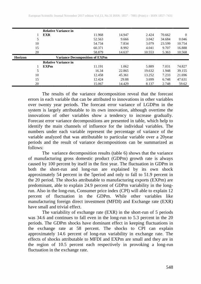
The results of the variance decomposition reveal that the forecast

errors in each variable that can be attributed to innovations in other variables

over twenty year periods. The forecast error variance of LGDPm in the

system is largely attributable to its own innovation, although overtime the

innovations of other variables show a tendency to increase gradually.

Forecast error variance decompositions are presented in table, which help to

identify the main channels of influence for the individual variables. The

numbers under each variable represent the percentage of variance of the

variable analyzed that was attributable to particular variable over a 20year

periods and the result of variance decompositions can be summarized as

follows:

The variance decomposition results (table 6) shows that the variance

of manufacturing gross domestic product (GDPm) growth rate is always

caused by 100 percent by itself in the first year. The fluctuation in GDPm in

both the short-run and long-run are explained by its own shock

approximately 54 percent in the 5period and only to fall to 51.9 percent in

the 20 period. The shocks attributable to manufacturing exports (EXPm) are

predominant, able to explain 24.9 percent of GDPm variability in the long-

run. Also in the long-run, Consumer price index (CPI) will able to explain 12

percent of fluctuation in the GDPm. While other variables like

manufacturing foreign direct investment (MFDI) and Exchange rate (EXR)

have small and trivial effect.

The variability of exchange rate (EXR) in the short-run of 5 periods

was 34.6 and continues to fall even in the long-run to 5.3 percent in the 20

periods. The GDPm shocks have dominant effect in keeping fluctuations in

the exchange rate at 58 percent. The shocks to CPI can explain

approximately 14.6 percent of long-run variability in exchange rate. The

effects of shocks attributable to MFDI and EXPm are small and they are in

the region of 10.5 percent each respectively in provoking a long-run

fluctuation in the exchange rate.


549

Consumer price index (CPI) in the short-run explained largely by its

own shock, however, in the long-run, its effects will decrease. In the long-

run, shocks to manufacturing exports (EXPm) and Manufacturing gross

domestic product (GDPm) are predominantly able to explain 40 percent and

24 percent respectively of CPI variability. The shocks to MFDI are

significantly able to explain 12 percent of fluctuations in the price level.

While the shocks to exchange rate have are small and trivial effects on price

level.

The variability of manufacturing exports (EXPm) in the short-run and

long-run are associated mainly with its own shock, 74.8 percent and 59.6

percent in the both short-run and long-run respectively. The exchange rate

shocks and shocks attributable to MFDI are just 27 percent 8.1 percent of

long-run fluctuation in manufacturing exports. The shocks of CPI shocks to

GDPm are in the region of 14.4 percent and 15 percent respectively.

In the case of MFDI, the variability of MFDI in the short-run is

associated mainly with its own shock and the shocks are very significant.

The effects of its own shock in the long-run are very small to the region of

only 6 percent. The shocks attributable to GDPm are very significant in the

long-run to cause fluctuations in the MFDI with 58.8 percent. The shocks

attributable to CPI are also high, able to explain 14.6 percent of fluctuations

in the MFDI. While the shocks attributable to other variables like exchange

rate and manufacturing exports are 5.3 percent and 10.5 percent respectively.

From the above results, it is quite evident that following conclusion

can be made:

i) The result indicates that GDPm is the most exogenous variables in the

system with only 39 percent of its forecast error variance being

explained by other variables, while about 61 percent of the forecast

error is attributable to its own shock.

ii) The result also shows that LEXR is the most interactive variable in the

system because 95 percent of its forecast error variances are explained

by LGDPm (58 percent), LCPI (14 percent), LEX (10 percent) and

LEXR (5 percent).

iii) It is therefore strengthen the evidence of causality that move from

LGDPm to MFDI i.e (LGDPm LMFDI).

5.3 Impulse Response Functions

Impulse Response Functions (IRFs) are one of the useful tools of the

unrestricted VAR approach for examining the interaction between the

variables in this study. They reflect how individual variables respond to

shocks from other variables in the system. When graphically presented, the

IFRs give a visual representation of the behavior of variables in response to

shocks. The responses are for a particular variable in the system. As noted by


550

Odusola and Akinlo, (2001), the interpretation of the impulse response

functions takes into consideration the first differencing of the variables as

well as the vector error correction estimates. The response forecast period is

50 years to enables us capture both the long-term and short-term responses.

The results can be presented in the figure 2 below:

-400,000

-200,000

0

200,000

400,000

600,000

5 10 15 20

Response of GDPM to GDPM

-400,000

-200,000

0

200,000

400,000

600,000

5 10 15 20

Response of GDPM to CPI

-400,000

-200,000

0

200,000

400,000

600,000

5 10 15 20

Response of GDPM to MFDI

-400,000

-200,000

0

200,000

400,000

600,000

5 10 15 20

Response of GDPM to EXR

-400,000

-200,000

0

200,000

400,000

600,000

5 10 15 20

Response of GDPM to REXP

-80

-40

0

40

80

5 10 15 20

Response of CPI to GDPM

-80

-40

0

40

80

5 10 15 20

Response of CPI to CPI

-80

-40

0

40

80

5 10 15 20

Response of CPI to MFDI

-80

-40

0

40

80

5 10 15 20

Response of CPI to EXR

-80

-40

0

40

80

5 10 15 20

Response of CPI to REXP

-200,000

-100,000

0

100,000

200,000

300,000

5 10 15 20

Response of MFDI to GDPM

-200,000

-100,000

0

100,000

200,000

300,000

5 10 15 20

Response of MFDI to CPI

-200,000

-100,000

0

100,000

200,000

300,000

5 10 15 20

Response of MFDI to MFDI

-200,000

-100,000

0

100,000

200,000

300,000

5 10 15 20

Response of MFDI to EXR

-200,000

-100,000

0

100,000

200,000

300,000

5 10 15 20

Response of MFDI to REXP

-80

-40

0

40

80

120

5 10 15 20

Response of EXR to GDPM

-80

-40

0

40

80

120

5 10 15 20

Response of EXR to CPI

-80

-40

0

40

80

120

5 10 15 20

Response of EXR to MFDI

-80

-40

0

40

80

120

5 10 15 20

Response of EXR to EXR

-80

-40

0

40

80

120

5 10 15 20

Response of EXR to REXP

-150,000

-100,000

-50,000

0

50,000

100,000

5 10 15 20

Response of REXP to GDPM

-150,000

-100,000

-50,000

0

50,000

100,000

5 10 15 20

Response of REXP to CPI

-150,000

-100,000

-50,000

0

50,000

100,000

5 10 15 20

Response of REXP to MFDI

-150,000

-100,000

-50,000

0

50,000

100,000

5 10 15 20

Response of REXP to EXR

-150,000

-100,000

-50,000

0

50,000

100,000

5 10 15 20

Response of REXP to REXP

Response to Cholesky One S.D. Innovations

Figure 2: Generalized Impulse Response

Dynamic movements of each to one standard error shock to each

other variables, particularly to the manufacturing gross domestic products

(GDPm) are analyzed by using orthogonalised impulse response functions

(IFRs) presented in figure below. According to the findings presented above,

a one standard error shock to GDPm will leads to the expansion of

manufacturing output in the long-run, since the effect of the shock on GDPm

will be positive.


551

The response of GDPm due to shock in CPI is positive up to 15 years

period, but after that it is expected to become negative. By implication, price

level is expected to decrease with the expansion in the manufacturing output

in the long-run. While a standard shock to GDPm will lead to an increase in

price level.

Furthermore, a standard error shock to GDPm leads to a positive

effect on manufacturing foreign direct investment (MFDI) in the long-run.

This tends to support the causality that runs from GDPm to MFDI. The

market size of the economy as represented by the GDP has been one of the

major determinants of FDI flow into the sector. While a standard error shock

to MFDI leads to fall in the manufacturing output in the long-run.

In addition, the response of exchange rate (EXR) due to shock to

GDPm is quite stable in the short-run, but become positive in the long-run.

While the response of the GDPm due to shock to EXR become negative in

the long-run. By implication, a one standard error shock to GDPm will lead

to a depreciation of domestic exchange rate and as Nigeria economy is more

open, the use of foreign reserve to cover current account deficit can lead to

the depreciation of Naira exchange rate.

Finally, a one standard error shock to manufacturing exports (EXPm)

will lead to a decrease in the GDPm in the long-run. While a response of

manufacturing exports due to shock to GDPm is positive in the long-run.

This result confirms the effectiveness of government’s industrial and export

incentives that were directed towards aiding exports in the manufacturing

exports.

6.0 Policy Implication and Recommendations

Generally speaking, the manufacturing sector plays a catalytic role in

a modern economy and has many dynamic benefits critical for economic

transformation. In any advanced economy or even growing economy like

Nigeria, the manufacturing sector is a leading sector in many respects. It is a

pathway for increasing national out-put in relation to import replacement and

export expansion, creating foreign exchange earning capacity, raising

employment and per capita income which causes unique consumption

patterns. In this study, it has been established that improvement in the out-

put growth in manufacturing sector will impact positively in the FDI flows

into the sector. To this end, efforts should be made by the government

through monetary and fiscal policies designed to boost out-put in the sector.

More so, efforts should be made to intensified the regulation of foreign

exchange market, since foreign exchange allocation play a crucial role in the

manufacturing out-put growth, efforts towards deregulation of the exchange

rate allocation to non-oil exports, especially to manufacturing sector, though

made the sector more competitive, but resulted in massive escalation of cost


552

in the procurement of industrial inputs and this negatively affect

manufacturing out-put. In addition, efforts should be made to make industrial

climate more conducive for manufacturing activities. These include

provision of basic infrastructural facilities that will enhance full utilization of

industrial capacity. This conducive atmosphere will motivate the flow of

foreign direct investment into the sector.

References:

1. Aiten, B. J., and Harrison, E. (1999), Do Domestic Firms Benefits

from Direct Foreign Investment? Evidence from Venezuela. The

American Economic Review, 89(3), 605-618.

2. Akinlo, A. E. (2004), Foreign Direct Investment and Growth in

Nigeria: An Empirical Investigation, Journal of Policy Modeling,

26(5),627-639.

3. Asiedu, E. (2002), Capital Controls and Foreign Direct Investment,

World Development, 32(3), 107-119.

4. Asiedu, E. (2001), On the Determinants of Foreign Direct

Investments to Developing Countries: Is Africa different? World

Development, 30(1),107-119.

5. Adenikinju, A. F. and Chete, L. N. (2002), Productivity, Market

Structure and Trade Liberalization in Nigeria. African Economic

Research Consortium (AERC), Research Paper, African Economic

Research Centre, Nairobi.

6. Aliber, R. Z. (1970), A Theory of Direct Foreign Investment. In The

International Corporation, Charles P. (Ed). Massachusetts: The MIT

press.

7. Aliber, R.Z (1971), The Multinational Enterprise in a Multiple

Currency World, In The Multinational Enterprise, J. H. Dunning

(Ed). London: George Allen and Unwin Ltd.

8. Akinlo, A. E, (2003), Exchange Rate Depreciation and Currency

Substitution in Nigeria, African Review of Money Finance and

Banking, 85(3),139-143.

9. Alvarez, R., (2003), Inversion extranjeradirecta on Chile y

suImpactoSobre la productividad.Departmento de Economia.

Universidad de Chile. Retrieved May 19, 2004.From

http/www.personal.ander. Ucla.Edu/Roberto.alvarez/paper IED. Pdf.

10. Bayoumi, T. and Eichengree B., (1994). Macroeconomic Adjustment

under Bretton Woods and the post Bretton-Woods Float: an Impulse

Response Analysis. The Economic Journal, (104), 813-827.

11. Buckley, P. J. (1985), A Critical View of The Theories of the

Multinational Enterprise. In the Economic Theory of Multinational


553

Enterprise, Buckley, P. J and M. Casson (ed.), New York: St Martin’s

Press.

12. Buckley, P. J. (1990), Problems and Developments in the Core

Theory of International Business, Journal of International Business

Studies, 21(4), 657-665.

13. Central Bank of Nigeria, (2010), Statistical Bulletins, Abuja, Nigeria.

14. Coase, R. H. (1937), The Nature of the Firm, Economica, 4(16),386-

405.

15. Chirwa, E. W. and Zakeyo, C. (2003), Impact of Economic and Trade

Policy Reforms on Food Security in Malawi, Report Submitted to the

Food and Agricultural Organisation FAO), Lilongwe, Malawi and the

Africa Economic Research Consortium, AERC.

16. Caves, R. E. (1971), International Corporations: The Industrial

Economics of Foreign Investment, Economica, 38(149),1-27.

17. Caves, R. E. (1974), Multinational Firms, Competition and

Productivity in the Host Country Markets, Economica, 41(162),176-

193.

18. Chete, L. N. Adeoti, J. O., Adeyinka, F. M. and Ogundele, O. (2013),

Industrial Development and Growth in Nigeria, Working Paper No.8,

Africa Growth Initiative at Brookings, African Development Bank

Group and United Nations University UNU-WIDER.

19. Dadush, U., Dasgupta, D. and Ratha, D. (2000), The Role of Short-

term Debt in Recent Crises, Finance and Development, 37(4), 54-57.

20. Dunning, J, H. (1977), Trade, Location of Economic Activity and the

MNE: A Search for an Eclectic Approach: In The International

Allocation of Economic Activity, Bertil Ohlin et al (Eds). London:

Macmillan.

21. Dunning, J. H. (1979), Explaining Changing Patterns of International

Production: Some Empirical Tests, Journal of International Business

Studies,11(1),9-31.

22. Dunning. J. H. (1988), Explaining the International Direct Investment

Position of Countries: Toward a Dynamic or Developmental

Approach, WeltwirtchaftHichesArhiv 119(1), 30-64.

23. De Mello, L. (2002), Foreign Direct Investment-led growth:

Evidence from time series and Panel Data, Oxford Economic Papers

No. 51,133-151.

24. Dunning, J.H.(1993), Multinational and the global economy, Addison

Wesley: Wokingham, England.

25. Ekanayake, E. M., Richard, V. and Veeramacheneni, B. (2003),

Openness and Economic Growth: Empirical Evidence on the

Relationship between Output, Inward FDI and Trade, Journal of

Business Strategies, 20(1),59-72.


554

26. Gokal, V. and Hanif, S. (2004), Relationship between Inflation and

Economic Growth, , Economic Department, Reserve Bank of Fiji,

Suva, Fiji, Working Paper No. 002.

27. Grosse, R. and Kujawa, D. (1995), International Business: Theory

and Managerial Application. U.S: Irwin.

28. Haddad M. and Harrison A. (1993), Are there Positive Spillovers

from Direct Foreign Investment? Evidence from Panel Data for

Morocco, Journal of Development Economics, 42(1),51-74.

29. Inegbenebor, A. O. (1995), Size, Structure and Performance of

Private Nigerian Manufacturing Enterprises: Nigerian Journal of

Economics and Social Studies, 37(1), 13-27.

30. Kojima, K. (1973), A Macroeconomic Approach to Foreign Direct

Investment, Hitotsubashi Journal of Economics, 14(1), 1-21.

31. Kojima, K. (1984), Micro-and Macro Economic Models of Foreign

Direct Investment: Towards a synthesis, Histosubashi, Journal of

Economics, 25(1), 1-20.

32. Kindleberger, C. P. (1984), Multinational Excursions, Cambridge,

Mass: MIT Press.

33. Karbasi, A. E., Mahamadi, E.andGbofrani, S. (2005), Impact of

Foreign Direct Investment on Economic Growth, Paper Presented at

the 12th Economic Research Forum Conference, 19th-21st December,

Egypt.

34. Kohpaiboon, A. (2004), Foreign Trade Regimes and the FDI-Growth

Nexus: A Case Study of Thailand, Journal of development studies,

40(2),55-69.

35. Lipsey, R. E. (2001), Foreign Direct Investment and Wages in

Indonesian Manufacturing, NBER, Working Paper No. 8299.

36. Lipsey, R. and Sjoholm, F. (2004), Foreign Direct Investment

Education and Wages in Indonesian Manufacturing, Journal of

Development Economics, 73(1),415-422.

37. Mansouri, B. (2005), The Interactive Impact of FDI and Trade

Openness on Economic Growth: Evidence from Morocco, Paper

Presented at the 12th Economic Research Forum (ERF) Conference,

Cairo, December.

38. Morisset, J. (2000), Foreign Direct Investment in Africa: Policy also

Matters, Transitional Corporations, 9(2),107-125.

39. Odusola, A. F. and Akinlo, A. E. (2001), Output, Inflation and

Exchange Rate in Developing Countries: An Application to Nigeria,

The Developing Economics, 39(2),39-42.

40. Okonjo-Iweala, N. and Osafo-Kwaako, P. (2007), Nigeria’s

Economic Reforms: Progress and challenges, Brookings Global


555

Economy and Development, The Brookings Institution, Washington,

DC 20036.

41. Oscar, B. and Simon, S. R. (1994), An Econometric Analysis of

Foreign Investment in Spain, 1964-1989, Southern Economic

Journal, 16(1), 104-120.

42. Oyelaran-Oyeyinka, B. (1997), Technological Learning in African

Industry, A Study of Engineering Firms in Nigeria, Science and

Public Policy, 24(5),309-318.

43. Ratha, D. (2000), Complementarity between Multilateral Lending

and Private Flows to Developing Countries: Some Empirical Results,

Policy Research, World Bank Working Paper No. 2746.

44. Rettab, B. Rao, A. and Charif, H. (2009), Why Do Firms Venture in

External markets?The case of Dubai, International Research, Journal

Finance and Economics, 29(1), 146-159.

45. Rugman, A. M. (1979), International Diversification and the

Multinational Enterprise, Lexington, KY: D.C Health.

46. Sun, H. (1996), Macro-Economic Impact of Direct Foreign

Investment in China:1977-1993, Department of Economics,

University of Sydney, Australia. Working Papers in Economics, No

232.

47. Ubok-Udom, E. (1999), Currency Depreciation and Domestic Output

Growth in Nigeria, The Nigeria Journal of Economics and Social

Studies, 5(5),1-12.

48. Venon, R. (1979), International Investment and International Trade in

the Product Life Cycle, Quarterly Journal of Economics, 80(1),190-

207.


556

Table 6: Generalized Variance Decomposition (VDCs) results

Variance Decomposition of GDPm

Horizon

GDPm

CPI

MFDI EXR EXPm

1

Relative Variance

in GDPm 100 0 0 0 0

5

54.356 35.974 5.647 3.122 0.902

10

34.486 38.486 6.021 2.9 18.107

15

37.402 16.798 2.41 3.771 39.619

20

51.936 12.22 6.288 4.618 24.939

Horizon

Variance Decomposition of CPI

1

Relative Variance

in CPI 11.283 88.717 0 0 0

5

20.509 64.911 9.468 1.648 3.464

10

4.133 47.306 4.557 4.154 39.85

15

13.614 17.79 2.263 2.927 63.405

20

24.901 17.701 12.126 3.087 40.186

Horizon

Variance Decomposition of MFDI

1

Relative Variance

in MFDI 0.096 0.906 98.998 0 0

5

46.458 27.982 17.847 3.83 3.884

10

50.163 26.827 7.286 3.04 12.683

15

53.211 12.854 4.035 4.608 25.292

20

62.929 11.697 6.115 5.02 14.24

Horizon

Variance Decomposition of EXR

1

Relative Variance

in EXR 11.968 14.947 2.424 70.662 0

5

52.563 9.666 3.042 34.684 0.046

10

54.734 7.834 3.079 23.599 10.754

15

60.371 8.992 4.041 9.707 16.888

20

58.879 14.637 10.553 5.363 10.568

Horizon

Variance Decomposition of EXPm

1

Relative Variance

in EXPm 11.191 1.062 5.889 7.031 74.827

5

16.34 22.865 19.632 1.948 39.155

10

12.458 45.361 13.252 7.233 21.696

15

12.424 29.88 3.699 6.748 47.631

20

15.067 14.429 8.137 2.748 59.62

the impact of foreign direct investment on the nigeria

Documents