the impact of h z in models with two scalar doublets
TRANSCRIPT

The impact of h→ Zγ in models with two scalardoublets
Duarte Sarmento de Sousa Machado Fontes
Thesis to obtain the Master of Science Degree in
Engineering Physics
Supervisors: Prof. Doutor Jorge Manuel Rodrigues Crispim Romão
Prof. Doutor João Paulo Ferreira da Silva
Examination Committee
Chairperson: Prof. Doutor Mário João Martins Pimenta
Supervisor: Prof. Doutor João Paulo Ferreira da Silva
Member of the Comittee: Prof. Doutor Rui Alberto Serra Ribeiro dos Santos
October 2014


“We are not to tell nature what she’s gotta be. (...)
She’s always got better imagination than we have.”
– Richard P. Feynman (1918-1988)
Today’s answers to Newton’s queries about light.
Sir Douglas Robb Lectures, University of Auckland (1979);
lecture 1, Photons: Corpuscles of Light.
i

ii
Acknowledgements
It would be a clear mistake to think this thesis results exclusively of my work and mine alone, for it
was the consequence of the joint work of my supervisors - Professors Jorge C. Romao and Joao Paulo
Silva - and myself. To them I am profundly indebted, not only for letting me be part of their team, but
mostly due to their charitable patience for listening and answering to my endless questions for a whole
year, regarding both physics as well as computational techniques. The integrity of their work and their
sense of commitment have overtaken all my (already high) expectations. The pedagogy and, above all,
the availability they have demonstrated are commendable. I owe them the (although small) insight I
gained in particle physics research and the opportunity to publish a scientific paper with them. I cannot
thank them both enough.
I want to thank my colleague Andre Patrıcio for helping me out in innumerable situations and for
keeping me alert for several interesting opportunities.
I would like to thank Professor Rui Santos for all the support given during our investigation and the
enlightening discussions.
I would also like to express my gratitude to Fundacao para a Ciencia e Tecnologia (FCT) and to
Centro de Fısica Teorica de Partıculas (CFTP), in particular to Professor Filipe Joaquim, for always
being available and for the encouragement he gave me in my last presentation.
I end up thanking Luıs Sombreireiro for the interesting discussions about the unitary gauge and Joao
Penedo for the help he gave me with several computational programs.
iii

iv

Este trabalho foi financiado pela Fundacao para a Ciencia e Tecnologia
(FCT), sob o contrato EXPL/FIS-NUC/0460/2013 no ambito do pro-
jecto de investigacao “Sinergia entre a Fısica do sabor e do LHC”.
This work has been financially supported by Fundacao para a Ciencia
e Tecnologia (FCT), under the grant EXPL/FIS-NUC/0460/2013 from
the research project “Sinergia entre a Fısica do sabor e do LHC ”.
v

vi

Resumo
A tao esperada descoberta do bosao de Higgs deu-se finalmente em 2012. Importa agora conhecer
as suas propriedades, em particular se se assemelha a partıcula de Higgs prevista pelo Modelo Padrao
da Fısica de Partıculas. Estas propriedades podem ser estudadas atraves dos seus decaimentos; neste
trabalho, focamo-nos no modo de decaimento h → Zγ, que e especialmente sensıvel a Nova Fısica, uma
vez que e mediado por um loop de partıculas. Este decaimento sera provavelmente observado na proxima
operacao do Large Hadron Collider a 14 TeV e pode assim trazer uma nova compreensao da Fısica do
Higgs.
Sabe-se actualmente que o Modelo Padrao esta incompleto; direccionamos assim o estudo de h→ Zγ
a uma das extensoes mais simples a esse modelo, o chamado 2 Higgs Doublet Model - tanto na versao que
conserva CP como na versao com violacao de CP -, que considera partıculas adicionais a contribuir para
os decaimentos. Exploramos a possibilidade de o bosao de Higgs ser uma mistura entre estados escalar
e pseudoescalar. Abordamos ainda a hipotese recente de o acoplamento de Yukawa entre o Higgs e um
par de quarks bottom ter o sinal contrario ao do Modelo Padrao.
Para alem dos referidos topicos, discutimos a renormalizacao do decaimento h → Zγ, a importancia
decisiva dos constrangimentos actuais a h → ZZ∗ e h → W+W− e os efeitos distintos das taxas de
producao.
Palavras-chave: bosao de Higgs; h→ Zγ; 2 Higgs Doublet Model; pseudoescalar;
sinal errado no acoplamento de Yukawa
vii

viii
Abstract
The long awaited discovery of the Higgs boson took place in 2012. It is now important to ascertain
its properties, in particular whether it resembles the Higgs particle predicted by the Standard Model
of Particle Physics. These properties can be studied through its decays; in this work, we focus on the
h → Zγ decay mode, which is very sensitive to New Physics since it is loop mediated. This decay will
probably be observed in the next Large Hadron Collider run at 14 TeV and may thus bring a new insight
in the Higgs physics.
The Standard Model is presently known to be incomplete. We therefore direct our study of the h→ Zγ
decay to one of the simplest extensions to that model, the so called 2 Higgs Doublet Model - both in
its CP conserving and CP violating versions -, which considers additional particles contributing to the
decays. We probe the possibility of the Higgs boson being a mixture between scalar and pseudoscalar
states. We also address the recent question of whether the Yukawa coupling between the Higgs and a
pair of bottom quarks can have the opposite sign to that of the Standard Model.
Besides the referred topics, we discuss the renormalization concerning h→ Zγ, the decisive importance
of the current bounds of h→ ZZ∗ and h→W+W− and the distinctive effects of the production rates.
Keywords: Higgs boson; h → Zγ; 2 Higgs Doublet Model; pseudoscalar; wrong
sign Yukawa coupling
ix

x
Contents
Acknowledgements iii
Resumo vii
Abstract ix
List of Figures xvi
List of Tables xvii
List of Abbreviations xix
1 Introduction 1
2 The Standard Model 5
2.1 Review of the Electroweak Structure of the SM . . . . . . . . . . . . . . . . . . . . . . . . 5
2.2 Higgs production mechanisms in the SM . . . . . . . . . . . . . . . . . . . . . . . . . . . . 9
2.3 The h→ Zγ decay in the SM . . . . . . . . . . . . . . . . . . . . . . . . . . . . . . . . . . 10
2.3.1 The diagrams . . . . . . . . . . . . . . . . . . . . . . . . . . . . . . . . . . . . . . . 10
2.3.2 The amplitudes . . . . . . . . . . . . . . . . . . . . . . . . . . . . . . . . . . . . . . 12
2.3.3 The decay width . . . . . . . . . . . . . . . . . . . . . . . . . . . . . . . . . . . . . 14
2.3.4 Analysis . . . . . . . . . . . . . . . . . . . . . . . . . . . . . . . . . . . . . . . . . . 17
2.3.5 Renormalization . . . . . . . . . . . . . . . . . . . . . . . . . . . . . . . . . . . . . 19
3 The (CP conserving) 2HDM 26
3.1 The Model . . . . . . . . . . . . . . . . . . . . . . . . . . . . . . . . . . . . . . . . . . . . 26
3.2 Constraints . . . . . . . . . . . . . . . . . . . . . . . . . . . . . . . . . . . . . . . . . . . . 30
3.3 Simulation procedure and introduction of the analysis . . . . . . . . . . . . . . . . . . . . 32
3.4 The h→ Zγ decay in the 2HDM . . . . . . . . . . . . . . . . . . . . . . . . . . . . . . . . 34
3.5 Relevant limits of the 2HDM . . . . . . . . . . . . . . . . . . . . . . . . . . . . . . . . . . 36
3.6 The parameter space and the wrong-sign Yukawa . . . . . . . . . . . . . . . . . . . . . . . 38
3.6.1 Comparing with previous results . . . . . . . . . . . . . . . . . . . . . . . . . . . . 38
3.6.2 The crucial importance of h→ V V and trigonometry . . . . . . . . . . . . . . . . 39
3.6.3 How production affects the rates . . . . . . . . . . . . . . . . . . . . . . . . . . . . 41
3.6.4 Predictions for the 14 TeV run . . . . . . . . . . . . . . . . . . . . . . . . . . . . . 45
3.6.5 Predictions for the Flipped 2HDM . . . . . . . . . . . . . . . . . . . . . . . . . . . 48
3.6.6 Conclusions . . . . . . . . . . . . . . . . . . . . . . . . . . . . . . . . . . . . . . . . 48
xi
4 The C2HDM 51
4.1 The Model . . . . . . . . . . . . . . . . . . . . . . . . . . . . . . . . . . . . . . . . . . . . 51
4.2 Constraints . . . . . . . . . . . . . . . . . . . . . . . . . . . . . . . . . . . . . . . . . . . . 54
4.3 The h→ Zγ decay in the C2HDM . . . . . . . . . . . . . . . . . . . . . . . . . . . . . . . 55
4.4 The parameter space and the wrong-sign Yukawa . . . . . . . . . . . . . . . . . . . . . . . 56
4.4.1 Type I model . . . . . . . . . . . . . . . . . . . . . . . . . . . . . . . . . . . . . . . 57
4.4.2 Type II model . . . . . . . . . . . . . . . . . . . . . . . . . . . . . . . . . . . . . . 58
4.4.3 Lepton Specific model . . . . . . . . . . . . . . . . . . . . . . . . . . . . . . . . . . 60
4.4.4 Flipped model . . . . . . . . . . . . . . . . . . . . . . . . . . . . . . . . . . . . . . 60
4.4.5 Wrong-sign h1bb couplings in Type II C2HDM . . . . . . . . . . . . . . . . . . . . 61
4.4.6 Conclusions . . . . . . . . . . . . . . . . . . . . . . . . . . . . . . . . . . . . . . . . 65
4.5 Feynman rules for a general model with two Higgs doublets . . . . . . . . . . . . . . . . . 65
A Further explanations in the 2HDM 70
A.1 Real and complex parameters; rephasing the fields . . . . . . . . . . . . . . . . . . . . . . 70
A.2 The condition for CP Violation in the C2HDM . . . . . . . . . . . . . . . . . . . . . . . . 71
A.3 The Z2 symmetry; the different types of 2HDM . . . . . . . . . . . . . . . . . . . . . . . . 71
A.4 FCNC at tree level in the 2HDM . . . . . . . . . . . . . . . . . . . . . . . . . . . . . . . . 73
A.5 Equivalence between the definitions of CP Violation . . . . . . . . . . . . . . . . . . . . . 74
B Useful formulae concerning Higgs production and decays 76
B.1 Higgs production expressions . . . . . . . . . . . . . . . . . . . . . . . . . . . . . . . . . . 76
B.2 Higgs decays expressions . . . . . . . . . . . . . . . . . . . . . . . . . . . . . . . . . . . . . 77
B.2.1 The h→ γγ case . . . . . . . . . . . . . . . . . . . . . . . . . . . . . . . . . . . . . 77
B.3 Relation between the Passarino-Veltman functions and other loop functions . . . . . . . . 79
B.3.1 The integrals for h→ γγ . . . . . . . . . . . . . . . . . . . . . . . . . . . . . . . . 79
B.3.2 The integrals for h→ Zγ . . . . . . . . . . . . . . . . . . . . . . . . . . . . . . . . 80
C Computational programs 81
xii

List of Figures
1.1 The Branching Ratios of the Higgs decays in the SM as a function of the Higgs mass, mh.
The mass of the recently discovered scalar is marked with a dotted line. . . . . . . . . . . 2
1.2 Left panel: observed 95% CL limits (solid black line) on the production cross section of
a SM Higgs boson decaying to Zγ, as a function of the Higgs boson mass, using 4.6fb−1
of pp collisions at√s = 7 TeV and 20.7fb−1 of pp collisions at
√s = 7 TeV. The median
expected 95% CL exclusion limits (dashed red line) are also shown. The green and yellow
bands correspond to the ±1σ and ±2σ intervals (ATLAS collaboration, Ref. [16]). Right
panel: the exclusion limit on the cross section times the branching fraction of a Higgs
boson decaying into a Z boson and a photon divided by the SM value (CMS collaboration,
Ref. [17]). . . . . . . . . . . . . . . . . . . . . . . . . . . . . . . . . . . . . . . . . . . . . . 3
2.1 The relevant production mechanisms. . . . . . . . . . . . . . . . . . . . . . . . . . . . . . . 9
2.2 The 1PI diagrams . . . . . . . . . . . . . . . . . . . . . . . . . . . . . . . . . . . . . . . . 11
2.3 The reducible diagrams . . . . . . . . . . . . . . . . . . . . . . . . . . . . . . . . . . . . . 11
2.4 Real and imaginary parts of the complex amplitudes YF and YG. . . . . . . . . . . . . . . 17
2.5 Comparison between the partial decay widths. . . . . . . . . . . . . . . . . . . . . . . . . 18
2.6 Comparison between the contributions of top quark and the total fermion mediated loop. 18
2.7 The behavior of the h→ Zγ, h→ γγ and h→ bb decay widths in the limit mh mZ . . . 19
2.8 The on-shell renormalization of the Zγ interaction. . . . . . . . . . . . . . . . . . . . . . . 22
2.9 The reducible diagrams mediated by an internal Z boson and the respective counterterm. 22
2.10 The mixing between G0 and γ in the on-shell condition. . . . . . . . . . . . . . . . . . . . 22
2.11 On-shell renormalization of the 1PI diagrams. . . . . . . . . . . . . . . . . . . . . . . . . . 23
2.12 Relation between the Zγ and the hZγ counterterms. . . . . . . . . . . . . . . . . . . . . . 24
2.13 The sum between the 1PI diagrams and the Z boson mediated reducible diagrams cancels
the divergences. . . . . . . . . . . . . . . . . . . . . . . . . . . . . . . . . . . . . . . . . . . 24
3.1 The new Feynman diagrams in the CP conserving 2HDM . . . . . . . . . . . . . . . . . . 35
3.2 Points from the SET representing the squared moduli of C YG (black), kU YF top (blue),
kD YF bottom (red) and λYH (green) as a function of sin(β − α) for the Type II 2HDM. . . 36
3.3 Left panel: points from the SET obeying kD > 0 representing the interaction terms between
XW and Xt (blue), Xb (red) and XH± (green) divided by the squared modulus of XW , as
a function of sin(β − α). Right panel: the equivalent for γγ. . . . . . . . . . . . . . . . . . 36
3.4 Correlation between µZγ and µγγ for different values of m212 and for varying α. . . . . . . 37
xiii
3.5 Points from the SET representing the contribution of the charged scalar (with XH± =
λYH) both in the Zγ and γγ channels, for kD < 0 and kD > 0, as a function of the
charged scalar mass. . . . . . . . . . . . . . . . . . . . . . . . . . . . . . . . . . . . . . . . 38
3.6 Left panel: Assuming that all µf are within 20% of the SM prediction we plot µbb (red/dark-
gray) and µγγ (black). Right panel: Assuming now that µV V are within 5% of the SM
prediction we plot the same quantities. For comparison we also plot µbb (cyan/light-gray)
for the assumed production of Ref. [24]. . . . . . . . . . . . . . . . . . . . . . . . . . . . . 39
3.7 Left panel: Plot of tanβ as a function of sinα for all the points that obey Eq. 3.43 with
0.8 ≤ µV V ≤ 1.2. Right panel: Plot of sin2(β − α) as a function of tanβ for the points
that obey Eq. 3.43 with 0.8 ≤ µV V ≤ 1.2 and have kD < 0. . . . . . . . . . . . . . . . . . 40
3.8 Left panel: Fractional variation of sin2 (β − α) as a function of tanβ for all points with
kD < 0 that obey Eq. 3.43 with 0.8 ≤ µV V ≤ 1.2. Right panel: correlation between tan(α)
and tan(β) for all the points from the SET which obey 0.8 < µV V < 1.2. . . . . . . . . . . 40
3.9 Left panel: k2D as a function of sin2 (β − α) for all points with kD < 0 that obey Eq. 3.43
with 0.8 ≤ µV V ≤ 1.2 (black) or with 0.95 ≤ µV V ≤ 1.05 (cyan/light-gray). Right panel:
The same but for generated data obeying the model constraints. . . . . . . . . . . . . . . 41
3.10 Allowed region for k2D as a function of sin2 (β − α) for all points with kD < 0 that obey
0.8 ≤ µV V ≤ 1.2 (black). The region in cyan (light-gray) is obtained by imposing in
addition that 0.8 ≤ µττ ≤ 1.2, while in the region in red (dark-gray) we further impose
0.8 ≤ µγγ ≤ 1.2. . . . . . . . . . . . . . . . . . . . . . . . . . . . . . . . . . . . . . . . . . 42
3.11 Same as in Fig. 3.10, but for the assumed production rates in Ref. [24]. See text for details. 42
3.12 Left panel: Prediction for µτ+τ− (red/dark-gray) and µγγ (black) as a function of tanβ
for the LHC at 14 TeV with the constraint of 20% errors at 8 TeV. Right panel: Assuming
now that µV V are within 5% of the SM prediction at 14TeV, we plot the same quantities.
Also shown (cyan/light-gray) is the prediction for µbb(V h) from associated production. . . 45
3.13 Prediction for µτ+τ− (red/dark-gray), µZγ (cyan/light-gray) and µγγ (black) as a function
of tanβ, for the LHC at 14 TeV, with a measurement of µV V within 5% of the SM at 14
TeV. . . . . . . . . . . . . . . . . . . . . . . . . . . . . . . . . . . . . . . . . . . . . . . . . 46
3.14 Predictions for µZγ versus µγγ at 14 TeV, for kD < 0. In black, we have the points in
the SET (obeying theoretical constraints and S, T, U , only). In red/dark-gray (cyan/light-
gray), the points satisfying in addition V V within 20% (5%) of the SM, at 14 TeV. . . . . 47
3.15 Predictions for µZγ versus µγγ at 14 TeV, for kD > 0. In black, we have the points in
the SET (obeying theoretical constraints and S, T, U , only). In red/dark-gray (cyan/light-
gray), the points satisfying in addition V V within 20% (5%) of the SM, at 14 TeV. . . . . 48
xiv
3.16 Left panel: Allowed region for k2D as a function of sin2 (β − α) in the Flipped 2HDM, for
all points with kD < 0 that obey 0.8 ≤ µV V ≤ 1.2 (black). The region in cyan (light-gray)
is obtained by imposing in addition that 0.8 ≤ µττ ≤ 1.2, while in the region in red (dark-
gray) we further impose 0.8 ≤ µγγ ≤ 1.2. Right panel: Predictions for µZγ versus µγγ
at 14 TeV, for kD < 0, in the Flipped 2HDM. In black, we have the points in the SET
(obeying theoretical constraints and S, T, U , only). In red/dark-gray (cyan/light-gray),
the points satisfying in addition V V within 20% (5%) of the SM, at 14 TeV. Shown in
green/light-gray are the points satisfying µτ+τ− at 20% of the SM, which lie on a line going
diagonally from the origin with almost unit slope. . . . . . . . . . . . . . . . . . . . . . . . 49
4.1 Limits of CP conservation represented in the α2 − α3 plan (reproduction of Fig. 1 of
Ref. [60]). . . . . . . . . . . . . . . . . . . . . . . . . . . . . . . . . . . . . . . . . . . . . . 53
4.2 Points obeying bounded from below, perturbative unitarity and S, T, U constraints rep-
resenting the squared moduli of C YG (black), kU YF top (blue), kD YF bottom (red), λYH
(green), Ψt (purple) and Ψb (cyan) as a function of sin(β − (α1 − π/2)) for the Type II
2HDM. . . . . . . . . . . . . . . . . . . . . . . . . . . . . . . . . . . . . . . . . . . . . . . 56
4.3 Left panel: Results in the µZZ - µγγ plane (left panel) and in the µτ+τ− - µγγ plane (right
panel) for the Type I C2HDM. The points in green/light-gray, blue/black, and red/dark-
grey correspond to |s2| < 0.1, 0.45 < |s2| < 0.55, and |s2| > 0.85, respectively. . . . . . . . 57
4.4 Results in the µbb(V h) - µγγ plane (left panel) and in the µZγ - µγγ plane (right panel)
for the Type I C2HDM. The points in green/light-gray, blue/black, and red/dark-grey
correspond to |s2| < 0.1, 0.45 < |s2| < 0.55, and |s2| > 0.85, respectively. . . . . . . . . . . 58
4.5 Figures of µZγ (µγγ) on the left (right) panel, as a function of s2. The points in red/dark-
grey (cyan/light-grey) were chosen to obey µV V = 1 within 20% (5%). These figures have
been drawn for 14 TeV. . . . . . . . . . . . . . . . . . . . . . . . . . . . . . . . . . . . . . 59
4.6 Results in the µZZ - µγγ plane (left panel) and in the µτ+τ− - µγγ plane (right panel)
for the Type II C2HDM. The points in green/light-gray, blue/black, and red/dark-grey
correspond to |s2| < 0.1, 0.45 < |s2| < 0.55, and |s2| > 0.85, respectively. . . . . . . . . . . 59
4.7 Left panel: Type II results in the µZγ - µγγ plane. The points in red/dark-grey, blue/black,
and green/light-gray correspond to |s2| < 0.1, 0.45 < |s2| < 0.55, and |s2| > 0.85, respec-
tively. Right panel: Type II predictions in the µZγ - s2 plane. The points in red/dark-grey
(cyan/light-grey) were chosen to obey µV V = 1 within 20% (5%). This figure has been
draw at 14 TeV. . . . . . . . . . . . . . . . . . . . . . . . . . . . . . . . . . . . . . . . . . 60
4.8 Lepton Specific simulations in the µτ+τ− - µγγ plane. The points in green/light-gray,
blue/black, and red/dark-grey correspond to |s2| < 0.1, 0.45 < |s2| < 0.55, and |s2| > 0.85,
respectively. . . . . . . . . . . . . . . . . . . . . . . . . . . . . . . . . . . . . . . . . . . . 61
xv

4.9 Left panel: Flipped model results in the µτ+τ− - µγγ plane. The points in red/dark-
grey, blue/black, and green/light-gray correspond to |s2| < 0.1, 0.45 < |s2| < 0.55, and
|s2| > 0.85, respectively. Right panel: same as left, except that all values for s2 are
included as blue/black points. Also shown as red/dark-grey (cyan/light-grey) are those
points which obey µV V = 1 within 20% (5%). . . . . . . . . . . . . . . . . . . . . . . . . 61
4.10 Results of the simulation of Type II C2HDM on the sgn(C) sin (α1 − π/2)-tanβ (sinα-
tanβ) plane. In cyan/light-grey we show all points obeying µV V = 1.0±0.2; in blue/black
the points that satisfy in addition |s2|, |s3| < 0.1; and in red/dark-grey the points that
satisfy |s2|, |s3| < 0.05. . . . . . . . . . . . . . . . . . . . . . . . . . . . . . . . . . . . . . . 62
4.11 Results of the simulation of Type II C2HDM on the sgn(C) aD-sgn(C) bD plane of scalar-
pseudoscalar couplings of h1bb. On the left panel (right panel) we assume that the mea-
surements come from current data at 8 TeV (prospective data at 14 TeV) and are made
within 20% (5%) of the SM. Constraints from µV V are in cyan/light-grey, from µγγ are in
red/dark-grey, and from µτ+τ− are in blue/black. . . . . . . . . . . . . . . . . . . . . . . . 63
4.12 Results of the simulation of Type II C2HDM on the sgn(C) aU -sgn(C) bU plane of scalar-
pseudoscalar couplings of h1tt. On the left panel (right panel) we assume that the mea-
surements come from current data at 8 TeV (prospective data at 14 TeV) and are made
within 20% (5%) of the SM. Constraints from µZZ are in cyan/light-grey, from µγγ are in
red/dark-grey, and from µτ+τ− are in blue/black. . . . . . . . . . . . . . . . . . . . . . . . 63
4.13 Results of the simulation of Type II C2HDM on the sign(C) aD-λ plane. On the left
panel (right panel) we assume that the measurements come from current data at 8 TeV
(prospective data at 14 TeV) and are made within 20% (5%) of the SM. Constraints from
µV V are in cyan/light-grey; adding constraints from µτ+τ− (µγγ at 5%) only the points
in red/dark-grey survive; adding constraints from µγγ (µτ+τ− at 5%) only the points in
blue/black, survive. . . . . . . . . . . . . . . . . . . . . . . . . . . . . . . . . . . . . . . . . 64
xvi
List of Tables
1.1 Experimental results presented by ATLAS and CMS at ICHEP2014. . . . . . . . . . . . . 2
2.1 The χ0 coefficient of each reducible diagram. Their sum vanishes. . . . . . . . . . . . . . . 20
2.2 The χ1 coefficient of each reducible diagram. . . . . . . . . . . . . . . . . . . . . . . . . . 21
2.3 The χ1 coefficient of each 1PI diagram. . . . . . . . . . . . . . . . . . . . . . . . . . . . . 21
3.1 Values of a =ghffgSMhff
for each model and for the different fermions. . . . . . . . . . . . . . . 33
4.1 Couplings of the fermions to the lightest scalar, h1, in the form a+ ibγ5. . . . . . . . . . . 54
A.1 The couplings of the fermion singlets to the Higgs doublets in each model. . . . . . . . . . 72
A.2 The coefficients of the different fermionic fields in each model. . . . . . . . . . . . . . . . . 73
xvii

xviii

List of Abbreviations
1PI 1 Particle Irreducible
2HDM 2 Higgs Doublet Model
ATLAS A Toroidal LHC Apparatus
BSM Beyond the Standard Model
C2HDM Complex 2 Higgs Doublet Model
CDF Collider Detector at Fermilab
CL Confidence Level
CMS Compact Muon Solenoid
CP Charge-Parity
Eq. Equation
FCNC Flavour Changing Neutral Currents
Fermilab Fermi National Accelerator Laboratory
Fig. Figure
GeV Giga electron Volt
h.c. hermitian conjugate
LHC Large Hadron Collider
NNLO Next-to-Next-to-Leading Order
PDF Parton Distribution Function
QED Quantum Electrodynamics
Ref. Reference
SM Standard Model
TeV Tera electron Volt
vev vacuum expectation value
xix

xx

Chapter 1
Introduction
This thesis has been written having in mind a future student who might get interested in the subject
and decides to study it. My main goal is thus to be pedagogical. In every such work, I think it is
preponderant for the author to mention what he or she is assuming the reader knows, otherwise he or she
ends up explaining too much or too little. I am therefore assuming that the reader has some advanced
knowledge of Quantum Field Theory (including notions like radiative corrections, Rξ gauges, counter-
terms, Passarino-Veltman functions, Faddeev-Popov ghosts and gauge fixing terms1) and is acquainted
with the Standard Model of Particle Physics (in short, the Standard Model, or simply SM).
The research made for this thesis has lead to the publication of one paper and the submission for
publication of a second one - Refs. [1, 2] - with the authors Jorge C. Romao, Joao P. Silva and myself,
which are here combined in an integrated text. Hence I ask the reader not be angry if I constantly skip
between the first person of the singular and the plural: although this thesis has my name on it, the whole
work has been done as a team.
Several abbreviations will be repeatedly used throughout this thesis; if the reader starts to feel lost, a
list of the whole set of abbreviations is presented on page xix.
I would like to explain the reasons that lead me to study this subject and and its importance nowadays.
Since the discovery of a scalar neutral particle in 2012 with a mass close to 125 GeV confirmed by the
ATLAS [3] and CMS [4] collaborations from the LHC, the search for a deeper understanding on the Higgs
physics has gathered attentions all over the world. The CDF and D0 collaborations from FermiLab [5,6]
provided additional evidence on the discovery, and recent announcements made both by ATLAS [7] and
CMS [8] leave no doubt regarding the confirmation of such a particle2.
The scalar particle has been discovered through its decays to γγ, ZZ∗, WW ∗ and τ+τ− with errors
of order 20% (the several decay modes are presented in Figure 1.1). Decays into bb are only detected
at LHC and the Tevatron in connection with the associated V h production mechanism3, with errors of
order 50% [9, 10]. The experimental results for pp → h → f (where p represents a proton, h the Higgs
and f some final state) are usually presented in the form of ratios of observed rates to SM expectations,
1The last two of which will be less important.2This discovery has been an extraordinary success, since both the dominant production cross section (gluon-gluon fusion)
and the main channel of detection (γγ) occur only at 1 loop (as we shall see in Chapter 2).3This information shall be important in Chapters 3 and 4, although it now may seem obscure (the production mechanisms
will only be explained in Section 2.2))
1

10-5
10-4
10-3
10-2
10-1
100
40 60 80 100 120 140 160 180 200
Bra
nchin
g R
atios
mh (GeV)
h → b b-
h → c c-
h → τ τ−
h → µ µ−
h → W W*
h → Z Z*
h → γ γ
h → g g
h → Z γ
Figure 1.1: The Branching Ratios of the Higgs decays in the SM as a function of the Higgs mass, mh.The mass of the recently discovered scalar is marked with a dotted line.
which we call µf . The SM therefore corresponds to µf = 1 ∀f . For definiteness, our discussions will be
based on the ATLAS [11] and CMS [12] results presented in the plenary talks at ICHEP2014, which we
summarize in Table 1.1.
channel ATLAS CMS
µγγ 1.57+0.33−0.28 1.13± 0.24
µWW 1.00+0.32−0.29 0.83± 0.21
µZZ 1.44+0.40−0.35 1.00± 0.29
µτ+τ− 1.4+0.5−0.4 0.91± 0.27
µbb 0.2+0.7−0.6 0.93± 0.49
Table 1.1: Experimental results presented by ATLAS and CMS at ICHEP2014.
We note that ATLAS excludes the SM µγγ = 1 (µZZ = 1) at 2-σ (1-σ), while CMS is within 1-σ of the
SM on all channels. The discovered scalar is thus compatible with the SM Higgs boson (an interval of
2-σ is not sufficient to declare incompatibility). However, such an identification as the SM Higgs boson
is not certain yet4; indeed, from Table 1.1 we see that ATLAS shows a small excess of observed events in
the h → γγ channel. One possible explanation for such an excess considers additional charged particles
contributing to the loop which mediates the decay: such charged particles would participate at the same
perturbative order as those of the SM, making this decay a very sensitive one to new physics. In such a
scenario, another related decay for which the new charged particles would also contribute is the h→ Zγ.
Therefore, and despite being highly suppressed decays (see Fig. 1.1), the h→ γγ and h→ Zγ processes
might be preponderant in our understanding into possible Beyond the SM (BSM) models.
The h→ γγ decay, having been one of the channels through which the new particle has been discovered,
has already been studied using experimental data (see, for example, Refs. [13–15]). The h→ Zγ channel,
4Nevertheless, we shall henceforth refer to the newfound particle as a/the Higgs boson; the question which remains openis whether the discovered Higgs boson is unique and identical to the one predicted by the SM, h.
2

on the other hand, has not yet been observed, although there already exists an upper bound for h →Zγ,Z → l+l−, where l = e or µ: at 95% confidence level (CL) with a mass between 120 and 150 Gev
and between 120 and 160 GeV, the expected exclusion limits are represented in the left and right panels
of Fig. 1.2, according to the ATLAS and the CMS collaborations, respectively [16, 17]. These recent
Figure 1.2: Left panel: observed 95% CL limits (solid black line) on the production cross section of aSM Higgs boson decaying to Zγ, as a function of the Higgs boson mass, using 4.6fb−1 of pp collisionsat√s = 7 TeV and 20.7fb−1 of pp collisions at
√s = 7 TeV. The median expected 95% CL exclusion
limits (dashed red line) are also shown. The green and yellow bands correspond to the ±1σ and ±2σintervals (ATLAS collaboration, Ref. [16]). Right panel: the exclusion limit on the cross section timesthe branching fraction of a Higgs boson decaying into a Z boson and a photon divided by the SM value(CMS collaboration, Ref. [17]).
results therefore exclude models predicting µZγ to be larger than one order of magnitude above the SM
prediction, and will be enhanced in the future 14 TeV LHC run (Run2, by opposition to the recent 8 TeV
run Run1), establishing this decay as one of the very next experimental goals.
One of the simplest extensions to the SM considers not one but two Higgs doublets, while keeping the
remaining particle content and the symmetries of the model intact. It is the so-called 2 Higgs Doublet
Model (2HDM) [18], which naturally accommodates extra charged particles and therefore provides an
appealing scenario for the aforementioned excess of observed events. The 2HDM can be separated in
two major branches: the CP conserving 2HDM (also known as real 2HDM, or simply 2HDM) and the
CP violating 2HDM (also known as Complex 2HDM, or C2HDM5). The latter appears as an attempt to
answer the question of whether the newfound particle has some pseudoscalar component. In each of the
two models, we calculate the h→ Zγ decay width at one loop and we compare it with the one in the SM.
As the new models introduce new parameters, we investigate the region of the parameter space which is
still available for the models, given the current bounds imposed by the experiments.
Recently, the ATLAS and CMS collaborations have started ascertaining the values of the couplings
between the Higgs and the fermions [19, 20]. It has recently been emphasized by Carmi et al. [21], by
Chiang and Yagyu [22], by Santos [23] and by Ferreira et al. [24] that current data are consistent with
a lightest Higgs from the 2HDM which we will describe in Section 3.1 except that the coupling of the
bottom quark to that Higgs particle (hbb) has a sign opposite to that in the SM. We shall thus study this
possibility both in the 2HDM as in the C2HDM, emphasizing the role of the h→ Zγ.
5Strictly speaking, the model to which in here we call C2HDM pressuposes a softly broken Z2 symmetry (see Section3.1). Therefore, this dichotomy is abusive if this softly broken Z2 symmetry is not implicit.
3

In an attempt to be pedagogical, I have created Appendix A which has additional explanations re-
garding the 2HDM, so that a new student might easily learn the model using this thesis. It also seemed
important to present the Feynman rules relative to a general model with 2 Higgs Doublets - which can
yield the C2HDM, the 2HDM and the SM ones in the appropriate limits -, since they are preponderant
for the calculations throughout this work; they can be found in Section 4.5. Appendix B contains the
formulae concerning Higgs production and decays for a general model with two Higgs doublets (all but
the h → Zγ ones, which are written in the main text) and some othe relevant expressions, essential for
us to perform the numerical calculi. A final appendix describes the computational programs used in the
course of the research.
4
Chapter 2
The Standard Model
2.1 Review of the Electroweak Structure of the SM
Although I am assuming the reader has already studied the SM, I present here a brief review, which
shall be useful not only to properly understand the h → Zγ decay in this model, but also in order to
serve as a prelude for the models with 2 Higgs doublets, discussed in the subsequent chapters. I will be
following closely Refs. [25, 26].
The SM can be characterized by different sectors, as can be seen in the full Lagrangean:
LSM = Lgauge + Lfermions + LHiggs + LYukawa + LGF + Lghosts. (2.1)
Before we describe each term, let us focus on the general structure of the theory. The SM is invariant
under local transformations of the gauge group
SU(3)C ⊗ SU(2)L ⊗ U(1)Y , (2.2)
where the subscripts C, L and Y represent color, left-handedness and hypercharge, respectively, and has
the following gauge fields:
Bµ, W aµ (a = 1, 2, 3), Gkµ (k = 1...8), (2.3)
which correspond, respectively, to the U(1)Y gauge boson, the SU(2)L gauge bosons and the gluons.
Furthermore, the SM describes the interactions of:
• quarks, represented by pR [0, 2/3], nR [0,−1/3] and qL =
pLnL
[1/2, 1/6]
[−1/2, 1/6]
,
• leptons, represented by CR [0,−1] and LL =
νLCL
[1/2,−1/2]
[−1/2,−1/2]
,
• Higgs boson, represented by Φ =
φ+
φ0
[1/2, 1/2]
[−1/2, 1/2]
,
where the indices L and R represent Left and Right, respectively, and the values inside the square brackets
express the electroweak quantum numbers [T3, Y ], which are such that Q = T3 + Y , where Q represents
5

the charge (in units of the charge of the proton), T3 the numerical value of the third component of the
weak isospin and Y the weak hypercharge value.
We are now in a position to analyze each term in Eq. 2.1. The first one has the following electroweak
structure1:
Lgauge = −1
4BµνB
µν − 1
4W aµνW
aµν , (2.4)
where
Bµν = ∂µBν − ∂νBµ, W aµν = ∂µW
aν − ∂νW a
µ − gεabcW bµW
cν , (2.5)
where g is the coupling constant relative to SU(2)L.
The second term, relative to the fermions, is given by
Lfermions = iqLγµD(qL)
µ qL + ipRγµD(pR)
µ pR + inRγµD(nR)
µ nR + iLLγµD(LL)
µ LL + iCRγµD(CR)
µ CR , (2.6)
where D(j) is the covariant derivative, which is given by the expressions
D(j)µ = ∂µ + i
g
2~τ . ~Wµ + i g′ Y (j)Bµ,
D(j)µ = ∂µ + i g Y (j)Bµ,
(2.7)
for the doublets and singlets of SU(2)L, respectively. The vector ~τ is composed of the 3 Pauli matrices
and g′ is the coupling constant relative to U(1). We are following the notation for the covariant derivatives
contained in Romao and Silva [25] with all ηs positive.
The term relative to the Higgs is
LHiggs = |D(Φ)Φ|2 + µ2(Φ†Φ)− λ(Φ†Φ)2 = |D(Φ)Φ|2 − V, (2.8)
where µ2 and λ are real parameters, and where the potential
V = −µ2(Φ†Φ) + λ(Φ†Φ)2 (2.9)
is responsible for the spontaneous symmetry breaking
SU(3)C ⊗ SU(2)L ⊗ U(1)Y −→ SU(3)C ⊗ U(1)EM (2.10)
and has its minimum correlated with the vacuum expectation value (vev) v according to
〈Φ†Φ〉 =v2
2=µ2
2λ. (2.11)
The fourth term, relative to the Yukawa interactions, is given by
LYukawa = −qLYdΦnR − qLYuΦ pR − LLYlΦCR + h.c., (2.12)
where Yd, Yu and Yl are (3 × 3) complex matrices containing the Yukawa couplings. I am using here a
very compact matricial notation: qL, nR, etc. are (3 × 1) vectors belonging to the family space. The
1We shall only focus on the electroweak part of the SM; in fact, in spite of being composed of color and electroweakparts, the former is completely independent of the latter, since the gauge bosons of those parts do not mix; the electroweakpart, on the other hand, cannot be separated into SU(2)L and U(1)Y , since the gauge bosons of both gauge groups aremixed together after the spontaneous symmetry breaking, as shall be clear in Eq. 2.16. We shall designate by LEW theLSM without the color part.
6
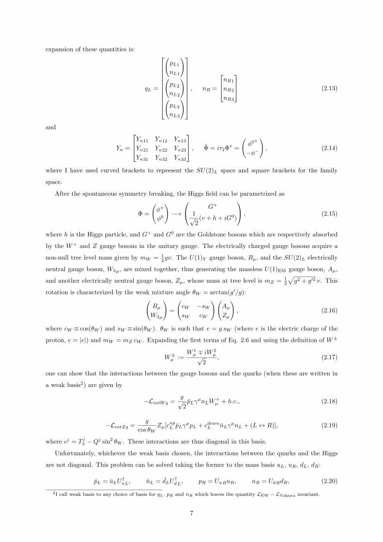
expansion of these quantities is:
qL =
(pL1
nL1
)(pL2
nL2
)(pL3
nL3
)
, nR =
nR1
nR2
nR3
(2.13)
and
Yu =
Yu11 Yu12 Yu13
Yu21 Yu22 Yu23
Yu31 Yu32 Yu33
, Φ = iτ2Φ∗ =
(φ0∗
−φ−
), (2.14)
where I have used curved brackets to represent the SU(2)L space and square brackets for the family
space.
After the spontaneous symmetry breaking, the Higgs field can be parametrized as
Φ =
(φ+
φ0
)−→
G+
1√2
(v + h+ iG0)
, (2.15)
where h is the Higgs particle, and G+ and G0 are the Goldstone bosons which are respectively absorbed
by the W+ and Z gauge bosons in the unitary gauge. The electrically charged gauge bosons acquire a
non-null tree level mass given by mW = 12gv. The U(1)Y gauge boson, Bµ, and the SU(2)L electrically
neutral gauge boson, W3µ, are mixed together, thus generating the massless U(1)EM gauge boson, Aµ,
and another electrically neutral gauge boson, Zµ, whose mass at tree level is mZ = 12
√g2 + g′2 v. This
rotation is characterized by the weak mixture angle θW = arctan(g′/g):(Bµ
W3µ
)=
(cW −sWsW cW
)(Aµ
Zµ
), (2.16)
where cW ≡ cos(θW ) and sW ≡ sin(θW ). θW is such that e = g sW (where e is the electric charge of the
proton, e = |e|) and mW = mZ cW . Expanding the first terms of Eq. 2.6 and using the definition of W±
W±µ :=W 1µ ∓ iW 2
µ√2
, (2.17)
one can show that the interactions between the gauge bosons and the quarks (when these are written in
a weak basis2) are given by
−LintWq =g√2pLγ
µnLW+µ + h.c., (2.18)
−LintZq =g
cos θWZµ[cupL pLγ
µpL + cdownL nLγµnL + (L↔ R)], (2.19)
where cj = T j3 −Qj sin2 θW . These interactions are thus diagonal in this basis.
Unfortunately, whichever the weak basis chosen, the interactions between the quarks and the Higgs
are not diagonal. This problem can be solved taking the former to the mass basis uL, uR, dL, dR:
pL = uLU†uL, nL = dLU
†dL, pR = UuRuR, nR = UdRdR, (2.20)
2I call weak basis to any choice of basis for qL, pR and nR which leaves the quantity LEW − LYukawa invariant.
7
where the unitary matrices U were chosen in order to diagonalize the Yukawa couplings:
MU := diag(mu,mc,mt) =v√2U†uLYuUuR, MD := diag(md,ms,mb) =
v√2U†dLYdUdR. (2.21)
In this new basis, and designating LH the section from the total Lagrangian which contains both the
mass terms of the quarks as well as the interaction between these and the Higgs, we have that
−LH = (1 +h
v)(uMUu+ dMDd), (2.22)
−LintWq =g√2uL(U†uLUdL)γµdLW
+µ + h.c., (2.23)
−LintZq =g
cos θWZµ[cupL uL(V V †)γµuL + cdownL dL(V V †)γµuL + (L↔ R)], (2.24)
where
V := U†uLUdL (2.25)
is the Cabibbo-Kobayashi-Maskawa (CKM) matrix. Eq. 2.23 allows flavour changing through charged
currents3. On the other hand, there is no flavour changing in the neutral currents (mediated by the Z
boson) - FCNC - due to the unitarity of the CKM matrix; in fact, since UuL and UdL are themselves
unitary matrices (implying V to be also unitary), we have that
V V † = 1 = V †V. (2.26)
It should still be noted that the interactions between the quarks and the W are purely left-handed, while
in the neutral currents there is no such restriction.
The fifth term from Eq. 2.1 has to do with the gauge fixing. Indeed, one needs to fix the gauge in
order to properly define the propagators. The term is given by
LGF = − 1
2ξGF 2G −
1
2ξAF 2A −
1
2ξZF 2Z −
1
ξWF−F+, (2.27)
where
F aG = ∂µGaµ, FA = ∂µAµ, FZ = ∂µZµ + ξZmZG0,
F+ = ∂µW+µ + iξWmWG
+, F− = ∂µW−µ − iξWmWG−,
(2.28)
where ξG, ξA, ξZ and ξW are arbitrary parameters.
Finally, the last term of the full Lagrangean concerns the ghosts, and it’s given by the Faddeev-Popov
prescription:
Lghosts =
4∑i=1
[c+∂(δF+)
∂αi+ c−
∂(δF−)
∂αi+ cZ
∂(δFZ)
∂αi+ cA
∂(δFA)
∂αi
]ci +
8∑a,b=1
ωa∂(δF aG)
∂βbωb, (2.29)
where ωa are the ghosts relative to SU(3), and c±, cA, cZ the ones relative to the electroweak part.
3The flavour changing was not possible in Eq. 2.18, i. e., the interaction was diagonal. The flavour changing is aconsequence of the requirement that the quarks have to be in a physical state (i. e., with well-defined mass).
8

2.2 Higgs production mechanisms in the SM
How is the SM Higgs boson produced in hadron machines like the LHC? An extensive review has
been done on this subject in Ref. [27]. In here, we would like to give a very short summary of the most
relevant topics for this thesis. In particular, I will focus on the production mechanisms.
When two protons collide, there are several possible interactions between their constituent particles
(quarks and gluons) that might originate a Higgs boson. In Fig. 2.1, we present the Feynman diagrams
regarding the relevant production mechanisms. They are, respectively, gluon-gluon fusion (gg → h),
associated production with heavy quarks (gg → h+qq), bb→ h4, V h associated production (qq → V + h,
where V = W orZ) and vector boson fusion (qq → V V ∗ + qq → h+ qq).
h
g
g
q
q
q
(a) Gluon-gluon fusion.
g
g
q h
q
q
(b) Associated production withquarks.
h
b
b
(c) bb→ h.
V
h
Vq
q
(d) V h associated production.
q
q
V ∗
V
h
(e) Vector boson fusion.
Figure 2.1: The relevant production mechanisms.
Since the couplings of the quarks to the Higgs are proportional to their masses (see Section 4.5), we
only consider the top and bottom quarks in the above diagrams. Moreover, we can practically neglect
the action of the bottom quark in the associated production with heavy quarks, without which this
mechanism may be called tth associated production.
All of the mechanisms - with the exception of bb → h - are considered in Ref. [27] to be dominant
in the SM. We also present bb → h since it will play an important role in the 2HDM. In the SM, the
mechanism with the most expressive contribution to the production cross section is the gluon-gluon fusion
(or simply gluon fusion) with an internal top quark - a loop mediated process.
In Chapters 3 and 4, we will calculate numerically the Higgs production. There are several useful
programs which compute the relative weight of the different production mechanisms; they generally allow
the user to choose the perturbative order at which he or she wants the computation to be made. We
use HIGLU [28] at next-to-next-to leading order (NNLO) for gluon-gluon fusion, SusHi [29] at NNLO for
4The equivalent processes with other quarks q (qq → h) give a negligible contribution.
9
bb→ h, and Ref. [30] for V h associated production, tth and vector boson fusion.
Another topic related to the Higgs production is the scale dependence of the masses. Due to radiative
corrections, the physical masses of the particles depend on the energy scale of the problem being studied.
We shall only take into consideration the QCD corrections and not the electroweak ones, since the latter
have not yet been programmed in HIGLU for the 2HDM; for the former, we use the next-to-nexto-to-
-leading order (NNLO). This means we only have to consider corrections to the quark masses. One should
thus ask to what energy scale should the masses be calculated in each case. In the Higgs production,
we do not consider radiative corrections explicitly - i.e., we use the pole masses - since these corrections
are already implemented inside HIGLU. By contrast, in the Higgs decay, we take the energy scale to be
mh5, following Ref. [27]6. The idea is that using this scale and the expression for the decay at tree level
we include a reasonable portion of the radiative corrections. In order to compute the quark masses at
different energy scales, we have made use of Eqs. 1.84 and 1.85 from Ref. [27] and Eq. 18 from Ref. [31].
2.3 The h→ Zγ decay in the SM
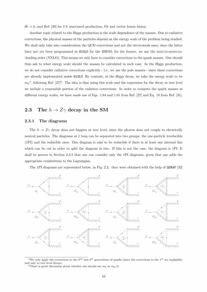
2.3.1 The diagrams
The h → Zγ decay does not happen at tree level, since the photon does not couple to electrically
neutral particles. The diagrams at 1 loop can be separated into two groups: the one-particle irreducible
(1PI) and the reducible ones. One diagram is said to be reducible if there is at least one internal line
which can be cut in order to split the diagram in two. If this is not the case, the diagram is 1PI. It
shall be proven in Section 2.3.5 that one can consider only the 1PI diagrams, given that one adds the
appropriate counterterm to the Lagrangian.
The 1PI diagrams are represented below, in Fig. 2.2; they were obtained with the help of QGRAF [32]
h
γ
Z
F1
h
γ
Z
F1a
kh
γ
Z
G1
kh
γ
Z
G1a
kh
γ
Z
G2
kh
γ
Z
G2a
kh
γ
Z
G3
kh
γ
Z
G3a
kh
γ
Z
G4
kh
γ
Z
G4a
kh
γ
Z
G5
kh
γ
Z
G5a
5We only apply the corrections to the 2nd and 3rd generations of quarks (since the corrections to the 1st are negligible)and only to tree level decays.
6There is great discussion about whether one should use mh or mh/2.
10
kh
γ
Z
G6
kh
γ
Z
G6a
kh
γ
Z
G7
kh
γ
Z
G7a
h
γ
Z
G8
h
γ
Z
G8a
h
γ
Z
G9
h
γ
Z
G9a
h
G10γ
k
Z
h
G10aγ
k
Z
h
Z
G11γ
kh
Z
G11aγ
k
h
Z
G12γ
h
Z
G13γ
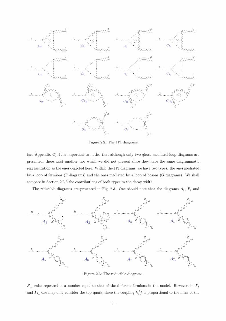
Figure 2.2: The 1PI diagrams
(see Appendix C). It is important to notice that although only two ghost mediated loop diagrams are
presented, there exist another two which we did not present since they have the same diagrammatic
representation as the ones depicted here. Within the 1PI diagrams, we have two types: the ones mediated
by a loop of fermions (F diagrams) and the ones mediated by a loop of bosons (G diagrams). We shall
compare in Section 2.3.3 the contributions of both types to the decay width.
The reducible diagrams are presented in Fig. 2.3. One should note that the diagrams A5, F1 and
h
γ
A1
Z
Z
h
γ
A2
Z
Z
h
γ
A3
Z
Z
h
γ
A4
Z
Z
h
γ
A5
Z
Z
h
γ
A6
Z
Z
h
γ
A7
Z
Z
h
γ
A7a
Z
Z
Figure 2.3: The reducible diagrams
F1a exist repeated in a number equal to that of the different fermions in the model. However, in F1
and F1a one may only consider the top quark, since the coupling hff is proportional to the mass of the
11
fermion(see Section 4.5), while the same is not true for A5.
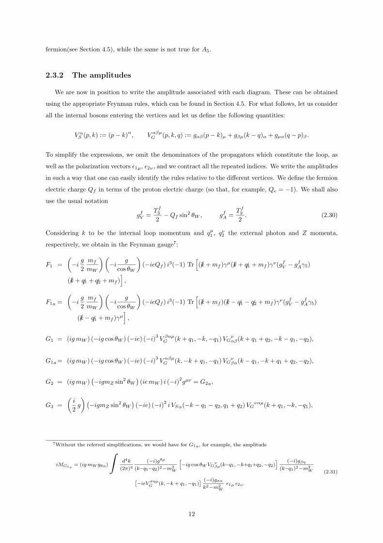
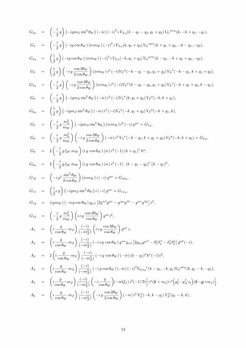
2.3.2 The amplitudes
We are now in position to write the amplitude associated with each diagram. These can be obtained
using the appropriate Feynman rules, which can be found in Section 4.5. For what follows, let us consider
all the internal bosons entering the vertices and let us define the following quantities:
V αS (p, k) := (p− k)α, V αβµG (p, k, q) := gαβ(p− k)µ + gβµ(k − q)α + gµα(q − p)β .
To simplify the expressions, we omit the denominators of the propagators which constitute the loop, as
well as the polarization vectors ε1µ, ε2ν , and we contract all the repeated indices. We write the amplitudes
in such a way that one can easily identify the rules relative to the different vertices. We define the fermion
electric charge Qf in terms of the proton electric charge (so that, for example, Qe = −1). We shall also
use the usual notation
gfV =T f32−Qf sin2 θW , gfA =
T f32. (2.30)
Considering k to be the internal loop momentum and qµ1 , qν2 the external photon and Z momenta,
respectively, we obtain in the Feynman gauge7:
F1 =
(−i g
2
mf
mW
)(−i g
cos θW
)(−ieQf ) i3(−1) Tr
[(/k +mf )γµ(/k + /q1 +mf )γν(gfV − gfAγ5)
(/k + /q1 + /q2 +mf )],
F1a =
(−i g
2
mf
mW
)(−i g
cos θW
)(−ieQf ) i3(−1) Tr
[(/k +mf )(/k − /q1 − /q2 +mf )γν(gfV − gfAγ5)
(/k − /q1 +mf )γµ],
G1 = (ig mW ) (−ig cos θW ) (−ie) (−i)3V βαµG (k + q1,−k,−q1)VG
ναβ(k + q1 + q2,−k − q1,−q2),
G1a= (ig mW ) (−ig cos θW ) (−ie) (−i)3V αβµG (k,−k + q1,−q1)VG
νβα(k − q1,−k + q1 + q2,−q2),
G2 = (ig mW )(−igmZ sin2 θW
)(iemW ) i (−i)2
gµν = G2a,
G3 =
(i
2g
)(−igmZ sin2 θW
)(−ie) (−i)2
i VSα(−k − q1 − q2, q1 + q2)VGναµ(k + q1,−k,−q1),
7Without the referred simplifications, we would have for G1a, for example, the amplitude
iMG1a= (ig mW gθα)
∫d4k
(2π)4
(−i)gθρ
(k−q1−q2)2−m2W
[−ig cos θWVG
νβρ(k−q1,−k+q1+q2,−q2)
] (−i)gβη(k−q1)2−m2
W[−ieV σηµG (k,−k + q1,−q1)
] (−i)gσαk2−m2
W
ε1µ ε2ν .
(2.31)
12
G3a =
(− i
2g
)(−igmZ sin2 θW
)(−ie) (−i)2
i VSα(k − q1 − q2, q1 + q2)VGανµ(k,−k + q1,−q1),
G4 =
(− i
2g
)(−ig cos θW ) (iemW ) (−i)2
i VSα(k, q1 + q2)VGαµν(k + q1 + q2,−k − q1,−q2),
G4a =
(i
2g
)(−ig cos θW ) (iemW ) (−i)2
i VSα(−k, q1 + q2)VGµαν(k − q1,−k + q1 + q2,−q2),
G5 =
(i
2g
)(−i g cos 2θW
2 cos θW
)(iemW ) i2 (−i)VSµ(−k − q1 − q2, q1 + q2)VS
ν(−k − q1, k + q1 + q2),
G5a =
(− i
2g
)(−i g cos 2θW
2 cos θW
)(iemW ) i2 (−i)VSµ(k − q1 − q2, q1 + q2)VS
ν(−k + q1 + q2, k − q1),
G6 =
(− i
2g
)(−igmZ sin2 θW
)(−ie) i2 (−i)VSν(k, q1 + q2)VS
µ(−k, k + q1),
G6a =
(i
2g
)(−igmZ sin2 θW
)(−ie) i2 (−i)VSν(−k, q1 + q2)VS
µ(−k + q1, k),
G7 =
(− i
2gm2h
mW
)(−igmZ sin2 θW
)(iemW ) i2 (−i) gµν = G7a,
G8 =
(− i
2gm2h
mW
)(−i g cos 2θW
2 cos θW
)(−ie) i3 VSν(−k − q1, k + q1 + q2)VS
µ(−k, k + q1) = G8a,
G9 = 2
(− i
2g ξW mW
)(i g cos θW ) (ie) i3 (−1) (k + q1)
νkµ,
G9a = 2
(− i
2g ξW mW
)(i g cos θW ) (ie) i3 (−1) (k − q1 − q2)
ν(k − q1)
µ,
G10 =
(−i g2 sin2 θW
2 cos θW
)(iemW ) i (−i) gµν = G10a,
G11 =
(i
2e g
)(−igmZ sin2 θW
)i (−i) gµν = G11a,
G12 = (igmW ) (−ieg cos θW ) gαβ[2gαβgµν − gαµgβν − gανgβµ
]i2,
G13 =
(− i
2gm2h
mW
)(i eg
cos 2θWcos θW
)gµνi2,
A1 =
(i
g
cos θWmZ
)(−i)
(−m2Z)
(i eg
cos 2θWcos θW
)gµν i,
A2 =
(i
g
cos θWmZ
)(−i)
(−m2Z)
(−i eg cos θW ) gανgαβ[2gσρg
µβ − δµσδβρ − δβσδµρ]gρσ(−i),
A3 = 2
(i
g
cos θWmZ
)(−i)
(−m2Z)
(−i g cos θW ) (−ie) (k − q1)µkν(−1)i2,
A4 =
(i
g
cos θWmZ
)(−i)
(−m2Z)
(−i g cos θW ) (−ie) (−i)2VGσρ
ν(k − q1,−k, q1)VGρσµ(k, q1 − k,−q1),
A5 =
(i
g
cos θWmZ
)(−i)
(−m2Z)
(−i g
cos θW
)(−ieQf ) i2(−1)Tr
[γµ(/k +mf )γν
(gfV−gfAγ5
)(/k− /q1+mf )
],
A6 =
(i
g
cos θWmZ
)(−i)
(−m2Z)
(−i g cos 2θW
2 cos θW
)(−ie) i2 V νS (−k, k − q1)V µS (q1 − k, k),
13
A7 =
(i
g
cos θWmZ
)(−i)
(−m2Z)
(−i g mZ sin2 θW
)(i emW ) i(−i)gµν = A7a.
2.3.3 The decay width
Kinematics
We can now turn to the decay width Γ. Initially we have8:
dΓ
dΩ=
1
32π2
|~q1|m2h
|M |2, (2.32)
where Ω is the solid angle, mh is the Higgs mass, q1 is the 4-momentum of the photon in the center of
mass frame and M is the total amplitude associated with the decay. If we now let√s be the center of
mass energy (or invariant mass), then√s = mh, in which case
|~q1| :=
√(s−m2
γ −m2Z
)2 − 4m2γm
2Z
2√s
=m2h −m2
Z
2mh, (2.33)
as mγ = 0, so that Eq. 2.32 becomes
dΓ
dΩ=
1
64π2
m2h −m2
Z
m3h
|M |2. (2.34)
Now, it is clear that the previous expression does not depend on the solid angle, the reason being that
there is no privileged direction (since the Higgs is a scalar particle). In fact, from the expression
q1.q2 =m2h −m2
Z
2, (2.35)
which comes directly from the momentum conservation equation (√s,~0) = q1 + q2, it is straightforward
to conclude that all the possible scalar products between the momenta are functions of the masses only,
in which case there are no angles. Eq. 2.34 thus becomes
Γ =1
16π
m2h −m2
Z
m3h
|M |2. (2.36)
Gauge invariance
The total amplitude can be written in the form
M = Mµνε1µε2ν , (2.37)
where we are just factorizing the polarization vectors ε1µ, ε2ν . Now, since the only structures in the
Lorentz space that can contribute to a second order tensor are the metric, the Levi-Civita alternating
symbol and the 4-momentum vectors, the Mµν term must have the form
Mµν = Agµν +B qµ1 qν2 + C qµ2 q
ν1 +Dqµ1 q
ν1 + E qµ2 q
ν2 + F εµναβq1αq2β , (2.38)
where A, B, C, D, E and F are scalar form factors. Since, for a certain particle i, we have that9
εi.pi = 0, (2.39)
8Eq. 3.145 from Ref. [33].9Eq. 3.262 from Ref. [34].
14
it then follows that B = D = E = 0, so that Eq. 2.38 becomes:
Mµν = Agµν + Cqµ2 qν1 + F εµναβq1αq2β . (2.40)
Now, due to gauge invariance, we have the relations10q1µMµν = 0
q2νMµν = 0
. (2.41)
Using Eq. 2.40, this expression can be rewritten asAq1ν + Cq1.q2 q1
ν = 0
Aq2µ + Cq1.q2 q2
µ = 0
, (2.42)
so that
A = −Cq1.q2, (2.43)
in which case, and using again Eq. 2.40, we have that
Mµν = C(−gµνq1.q2 + qµ2 qν1 ) + F εµναβq1αq2β . (2.44)
Using Eq. 2.37, we can at last conclude that gauge invariance implies that we can always write the
amplitude in the form
M = C (ε1.q2 ε2.q1 − ε1.ε2 q1.q2) + F εµναβq1αq2βε1µε2ν . (2.45)
Final expression
After computing the total amplitude for the decay using FeynCalc [35] (see Appendix C), we have
found that F = 0 in Eq. 2.45. This means we can write the total amplitude M as
M =g e2
16π2mW(ε1.ε2 q1.q2 − ε1.q2 ε2.q1) (YF + YG) , (2.46)
where we have decided to factorize the quantity g e2/(16π2mW ), and YF and YG are dimensionless
functions related to the fermion mediated loop and boson mediated loop amplitudes, respectively. As
it is implicit in Eq. 2.36, we have to sum over the polarizations, which we can do using the notation
ε1 = ε(λ1, q1) and ε2 = ε(λ2, q2):∑λ1,λ2
| ε1.q2 ε2.q1 − ε1.ε2 q1.q2|2
=∑λ1,λ2
(ε1.q2ε2.q1 − ε1.ε2q1.q2)∗
(ε1.q2ε2.q1 − ε1.ε2q1.q2)
=∑λ1,λ2
(ε∗µ1 ε∗2µ(q1.q2)
∗εα1 ε2αq1.q2 − ε∗µ1 ε∗2µ(q1.q2)
∗εα1 q2αε
β2 q1β − ε∗µ1 q∗2µε
∗ν2 q∗1νε
α1 ε2αq1.q2)
+ε∗µ1 q∗2µε∗ν2 q∗1νε
α1 q2αε
β2 q1β
)= (−gµα)(−gµα)|q1.q2|2 − (−gµα)(−δβα)(q1.q2)
∗q2αq1β − (−gµα)(−δνα)q∗2µq
∗1νq1.q2
+ (−gµα)(−gνβ)q∗2µq∗1νq2αq1β
10Eq. 3.211 from Ref. [34].
15
= 4 (q1.q2)2 − (q1.q2)
2 − (q1.q2)2
+ q22q
21
= 2 (q1.q2)2
=
(m2h −m2
Z
)22
,
(2.47)
where we have used q21 = 0, Eq. 2.35 and [34]∑
λ
εµ(k, λ)ε∗ν(k, λ) = −gµν . (2.48)
We can finally insert the expressions 2.46 and 2.47 in 2.36 to obtain
Γ =1
16π
m2h −m2
Z
m3h
(g e2
16π2mW
)2 (m2h −m2
Z
)22
|YF + YG|2
=1
32π
(1− m2
Z
m2h
)3(g e2
16π2mW
)2
|YF + YG|2
=GFm
3h
4π√
2
α2
16π2
(1− m2
Z
m2h
)3
|YF + YG|2,
(2.49)
where GF and α are the Fermi coupling and the fine-structure constants, respectively. Using now Feyn-
Calc, we can calculate YF and YG in terms of the Passarino-Veltman scalar functions [36,37]. The result
is:
YF =∑f
Nfc
Qf gfV
sin θW cos θWIF , YG =
1
tan θWIW , (2.50)
where the sum in f is made over all the fermion mediated loop diagrams; Nfc is the color number
associated with the fermion f ; the functions IF and IW are given by the expressions
IF=−8m2
fm2Z
(m2h −m2
Z)2
[B0
(m2h,m
2f ,m
2f
)−B0
(m2Z ,m
2f ,m
2f
)]+
4m2f
m2h −m2
Z
[−2 +
(−4m2
f +m2h
−m2Z
)C0
(m2Z , 0,m
2h,m
2f ,m
2f ,m
2f
) ],
(2.51)
IW=1
(m2h −m2
Z)2
[m2h
(1− tan2 θW
)− 2m2
W
(−5 + tan2 θW
) ]m2Z ∆B0 +
1
m2h −m2
Z
[m2h
(1
− tan2 θW)− 2m2
W
(−5 + tan2 θW
)+ 2m2
W
((−5 + tan2 θW
) (m2h − 2m2
W
)− 2m2
Z (−3+
tan2 θW))
C0
(m2Z , 0,m
2h,m
2W ,m
2W ,m
2W
) ],
(2.52)
where we used the short notation
∆B0 = B0
(m2h,m
2W ,m
2W
)−B0
(m2Z ,m
2W ,m
2W
). (2.53)
The functions IF and IW can also be calculated analytically [38], and the results are:
IF (τf , λf ) = −4[I1(τf , λf )− I2(τf , λf )
], (2.54)
IW (τW , λW ) = −4(3− tan2 θW
)I2(τW , λW )−
[(1 +
2
τ
)tan2 θW −
(5 +
2
τ
)]I1(τW , λW ), (2.55)
16
where τi = 4m2i /m
2h and λi = 4m2
i /m2Z , with i = f,W ; the functions I1 and I2 have the explicit form [38]:
I1(τ, λ) =τλ
2(τ − λ)+
τ2λ2
2(τ − λ)2 [f(τ)− f(λ)] +
τ2λ
(τ − λ)2 [g(τ)− g(λ)] , (2.56)
I2(τ, λ) = − τλ
2(τ − λ)[f(τ)− f(λ)] , (2.57)
where f and g are complex functions such that
f(x) =
arcsin2(
√1/x), x ≥ 1
−1
4
[log
1 +√
1− x1−√
1− x − iπ]2
, x < 1,(2.58)
g(y) =
√y − 1 arcsin(1/
√y),y ≥ 1
√1− y2
[log
1 +√
1− y1−√1− y − iπ
],y < 1.
(2.59)
We have checked that the two procedures - computational and analytical - yield the exact same result.
Other relations between Passarino-Veltman functions and analytical expressions are presented in the
Appendix B.3.2.
2.3.4 Analysis
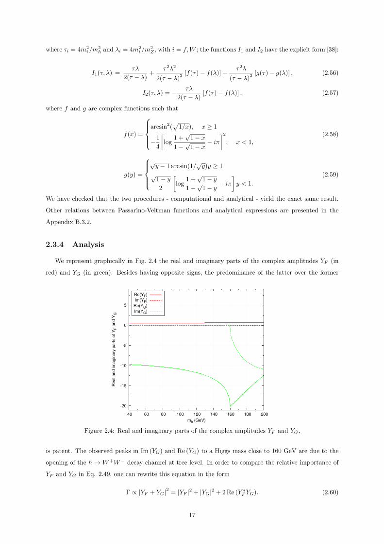
We represent graphically in Fig. 2.4 the real and imaginary parts of the complex amplitudes YF (in
red) and YG (in green). Besides having opposite signs, the predominance of the latter over the former
-20
-15
-10
-5
0
5
40 60 80 100 120 140 160 180 200
Real and im
agin
ary
part
s o
f Y
F a
nd Y
G
mh (GeV)
Re(YF)
Im(YF)
Re(YG)
Im(YG)
Figure 2.4: Real and imaginary parts of the complex amplitudes YF and YG.
is patent. The observed peaks in Im (YG) and Re (YG) to a Higgs mass close to 160 GeV are due to the
opening of the h→ W+W− decay channel at tree level. In order to compare the relative importance of
YF and YG in Eq. 2.49, one can rewrite this equation in the form
Γ ∝ |YF + YG|2 = |YF |2 + |YG|2 + 2 Re (Y ∗F YG). (2.60)
17

The comparison is presented in Fig. 2.5. It is again clear that the diagrams mediated by loops of fermions
(red line) have a much smaller contribution than the ones mediated by loops of bosons (green line). The
interference term between the two, 2 Re (Y ∗F YG) (blue line), has negative sign, which implies a destructive
-100
0
100
200
300
400
40 60 80 100 120 140 160 180 200
Part
ial decay w
idth
s
mh (GeV)
|YF|2
|YG|2
2 Re(YF* YG)
|YF + YG|2
Figure 2.5: Comparison between the partial decay widths.
interference. It should be noted that, within the diagrams mediated by loops of fermions, the top quark
mediated loop has the dominant contribution, since the coupling hff is proportional to the mass of the
fermion. This effect can be seen in Fig. 2.6.
0.3
0.35
0.4
0.45
0.5
40 60 80 100 120 140 160 180 200
Contr
ibutions to Y
F
mh (GeV)
Total
Only top
Figure 2.6: Comparison between the contributions of top quark and the total fermion mediated loop.
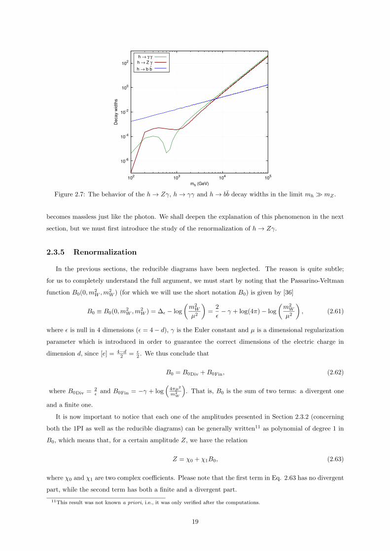
When we take the limit mh mZ , the h → Zγ decay width reduces to the h → γγ decay width,
except for a coupling factor. This effect can be seen in Fig. 2.7, where we also present the h→ bb decay
width for comparison. This phenomenon is explained by the fact that, since the reducible diagrams in
h→ Zγ can be neglected (see Section 2.3.5), the diagrams for both processes are the same (with the only
difference that one of the photons in h → γγ is replaced by a Z), so that, in the referred limit, the Z
18
10-6
10-4
10-2
100
102
102
103
104
105
Decay w
idth
s
mh (GeV)
h → γ γ
h → Z γ
h → b b-
Figure 2.7: The behavior of the h→ Zγ, h→ γγ and h→ bb decay widths in the limit mh mZ .
becomes massless just like the photon. We shall deepen the explanation of this phenomenon in the next
section, but we must first introduce the study of the renormalization of h→ Zγ.
2.3.5 Renormalization
In the previous sections, the reducible diagrams have been neglected. The reason is quite subtle;
for us to completely understand the full argument, we must start by noting that the Passarino-Veltman
function B0(0,m2W ,m
2W ) (for which we will use the short notation B0) is given by [36]
B0 ≡ B0(0,m2W ,m
2W ) = ∆ε − log
(m2W
µ2
)=
2
ε− γ + log(4π)− log
(m2W
µ2
), (2.61)
where ε is null in 4 dimensions (ε = 4− d), γ is the Euler constant and µ is a dimensional regularization
parameter which is introduced in order to guarantee the correct dimensions of the electric charge in
dimension d, since [e] = 4−d2 = ε
2 . We thus conclude that
B0 = B0Div +B0Fin, (2.62)
where B0Div = 2ε and B0Fin = −γ + log
(4πµ2
m2W
). That is, B0 is the sum of two terms: a divergent one
and a finite one.
It is now important to notice that each one of the amplitudes presented in Section 2.3.2 (concerning
both the 1PI as well as the reducible diagrams) can be generally written11 as polynomial of degree 1 in
B0, which means that, for a certain amplitude Z, we have the relation
Z = χ0 + χ1B0, (2.63)
where χ0 and χ1 are two complex coefficients. Please note that the first term in Eq. 2.63 has no divergent
part, while the second term has both a finite and a divergent part.
11This result was not known a priori, i.e., it was only verified after the computations.
19

We make here a quick return to the topic concerning the comparison between h → γγ and h → Zγ
in the limit mh mZ , discussed in the previous section. I think it is quite important to notice that
the equality (up to a constant factor) of their decay widths is only true because the set of diagrams
G8 +G8a +G13 becomes dominant as the Higgs mass grows12. This means we may write:
limmh→∞
∣∣∣∣XG
YG
∣∣∣∣2 = limmh→∞
∣∣Gγγ1 +Gγγ1a+Gγγ2 +Gγγ2a
+ ...∣∣2∣∣∣GZγ1 +GZγ1a
+GZγ2 +GZγ2a+ ...
∣∣∣2 ' limmh→∞
∣∣Gγγ8 +Gγγ8a+Gγγ13
∣∣2∣∣∣GZγ8 +GZγ8a+GZγ13
∣∣∣2
= limmh→∞
|2Gγγ8 +Gγγ13 |2∣∣∣2GZγ8 +GZγ13
∣∣∣2 = limmh→∞
∣∣∣∣∣ 2χγγ08
2χZγ08
∣∣∣∣∣2
=
ie(i g cos(2θW )
2 cos(θW )
)
2
= 2.459013 ,
(2.64)
where XG is the analogous to YG in the γγ decay and where we have used the relations G8 = G8a ,
χ013= 0 and 2χ08
= −χ013. We have also used the fact that, in the limit mh → ∞, the only difference
between χγγ08and χZγ08
is that, in the former, we have a coupling ϕ± ϕ∓γ, while in the latter we have
ϕ± ϕ∓Z. We then have:
limmh→∞
Γ(h→ γγ)
Γ(h→ Zγ)= limmh→∞
GFm3h
4π√
2
α2
16π2
1
2|XF +XG|2
GFm3h
4π√
2
α2
16π2
(1− m2
Z
m2h
)3
|YF + YG|2
=1
2lim
mh→∞|XF |2 + |XG|2 + 2 Re (XFX
∗G)
|YF |2 + |YF |2 + 2 Re (YFY ∗G)' 1
2lim
mh→∞|XG|2
|YG|2= 1.2295072 .
(2.65)
We have verified numerically this result, which corresponds to the referred constant factor.
We now return to where we were. We present in Table 2.1 the χ0 associated with each reducible
diagram, where we are taking tW ≡ tan θW . Since there is a common factor to the set of coefficients,
given by
S =cW e g2mW ε1.ε2
16π2, (2.66)
we can factorize this quantity out. One concludes that the sum of the χ0 in the reducible diagrams
vanishes, which means that the reducible diagrams as a whole have no finite contribution besides that
which is inherent in B0.
Diagram χ0/SA1 1− t2WA2 6A3 1A4 −7A5 0A6 −
(1− t2W
)A7 +A7a 0
Sum 0
Table 2.1: The χ0 coefficient of each reducible diagram. Their sum vanishes.
We now focus on the χ1 terms of the reducible diagrams; these are presented in Table 2.2, where S
is again factorized out in each term. From Eq. 2.63 and using the results from the previous Tables, we
12This is due to the fact that the three amplitudes G8, G8a and G13 are proportional to mh. This is also the reason whythis set of diagrams is gauge invariant by itself.
20

Diagram χ1/SA1 1− t2WA2 6A3 1A4 −9A5 0A6 −
(1− t2W
)A7 +A7a −2 t2W
Sum −2(1 + t2W
)Table 2.2: The χ1 coefficient of each reducible diagram.
conclude that
∑i= Reducible
Zi = −2(1 + t2W
)S B0 = −2
(1 + t2W
) cW e g2mW ε1.ε216π2
B0. (2.67)
This is the total contribution of the reducible diagrams. Although it might seem a rather uninteresting
result, it becomes crucial when one looks at the 1PI diagrams (Table 2.3): it cancels exactly with the
sum of the χ1 terms of the 1PI diagrams. This can be summarized in the following relation:
∑i= All
Zi =∑i= 1PI
χ0i. (2.68)
This result implies that the divergences of the whole set of diagrams at 1 loop cancel. The combined
results of Table 2.1 and Eq. 2.68 tell us that one might neglect the reducible diagrams - since their only
function is to cancel the χ1 terms of the 1PI diagrams - given that one adds the appropriate counterterm
(CT) to the Lagrangean,
CT = −2(1 + t2W
) cW e g2mW ε1.ε216π2
B0. (2.69)
In the end, there is no trace of B0: both its divergent and finite parts vanish. It seems important to
Diagrams χ1/SF1 + F1a 0
G1 +G1a 9
G2 +G2a 0
G3 +G3a −3/4
G4 +G4a (3/4)t2WG5 +G5a −(1/2)t2WG6 +G6a −(1/4)
(t2W − 1
)G7 +G7a 0
G9 +G9a −1/2G10 +G10a t2WG11 +G11a t2WG12 +G12a −6
G8 +G8a +G13 0
Sum 2(1 + t2W
)Table 2.3: The χ1 coefficient of each 1PI diagram.
understand at a deeper level the reason why the Z boson mediated reducible diagrams cancel exactly the
sum of the χ1 terms of the 1PI diagrams. In order to do so, we must study the renormalization of the
h→ Zγ decay.
21

First of all, one should remember that there is the need of a renormalization procedure even if there are
no infinities; in fact, the renormalization is required in order to properly define the physical quantities (the
regularization is the process which is only required when infinities are present). Secondly, it is usually
thought that there can only be counterterms for vertices which exist at tree-level in the Lagrangian.
However, this is not true for theories with spontaneous symmetry breaking, as we shall see below.
We will use the on-shell renormalization scheme, which requires the particles to be final states (i.e.,
with well defined mass) and defines the masses as being the poles of the propagators. One must start
by identifying all the countertems of the Lagrangean, which shall be defined from the normalization
conditions that one must impose to the fields.
We show in Fig. 2.8 the on-shell renormalization condition for the interaction between Z and γ, where
the shaded blob represents the sum of all 1PI diagrams to all orders and where the second term (with
Z γ
+γZ
= 0(for q2
1 = 0)
Figure 2.8: The on-shell renormalization of the Zγ interaction.
the cross) represents the counterterm for the interaction. From this figure, it follows that:
h
Z
γ
Z
+h
Z
γ
Z
= 0(for q2
1 = 0).
Figure 2.9: The reducible diagrams mediated by an internal Z boson and the respective counterterm.
There would also exist equivalent relations for the mixing between G0 and γ, but we have checked
G0γ
=h
Z
γ
G0
= 0(for q2
1 = 0)
Figure 2.10: The mixing between G0 and γ in the on-shell condition.
22

that this is identically null in the limit q21 = 0, in which case the respective counterterm is also null. This
implies that the h → Zγ decay diagrams mediated by an internal neutral Goldstone boson are null in
this limit (Fig. 2.10).
The on-shell conditions apply to the 1PI diagrams in the following way:
h
Z
γ
+h
Z
γ
= K(for q2
1 = 0, q22 = m2
Z
).
Figure 2.11: On-shell renormalization of the 1PI diagrams.
with K being some finite complex number. This is, in fact, the whole point of the regularization: to
guarantee that the counterterm for the irreducible diagrams cancels the divergences.
So far, we haven’t made much progress. The interesting conclusion comes when one understands that
the counterterms for both the 1PI diagrams (Fig. 2.11) and the internal Z boson mediated reducible
diagrams (Fig. 2.9) are related to each other. To prove this, we start with the relevant part of the
Lagrangian (obtained from the first term of Eq. 2.8):
L =1
8
(v2 + 2vh+ h2
) [g2W 3
µWµ3 + g′2BµB
µ − 2gg′W 3µB
µ]
+ ... (2.70)
To obtain the counterterms, one uses the transformations [39]:
W 3µ →Z
1/2W W 3
µ , g → Z−1/2W (g + δg)
Bµ → Z1/2B Bµ, g′ →Z−1/2
B (g′ + δg′)
h→ Z1/2h h, v → Z
1/2h (v + δv).
(2.71)
After using g′ = g tan(θW ) and Eq. 2.16, one gets:(g2W 3
µWµ3 + g′2BµB
µ − 2gg′W 3µB
µ)→
→ g2
cos2(θW )ZµZ
µ + 2gZµZµ[δg + δg′ tan2(θW )
]+ 2gZµA
µ [δg tan(θW )− δg′] ,(2.72)
which means that, although no interaction exists between Z and γ at tree level, there exists a counterterm
(order δ) which relates the two fields. Note that such a relation is only possible because the equation
g′ = g tan(θW ) is not verified at order δ, this is, δg′ 6= δg tan(θW ). In fact, δg and δg′ have been calculated
in Ref. [39] and their values are
δg′ = 0, δg = − 2g3
16π2B0. (2.73)
From Eqs. 2.70 and 2.72, we obtain the following part of the counterterms Lagrangean:
Lc =1
8
(v2 + 2vh
)2gZµA
µ [δg tan(θW )− δg′] + ...
=1
4v2g [δg tan(θW )− δg′]ZµAµ +
1
2vg [δg tan(θW )− δg′]hZµAµ + ...
= δZZγ + δZhZγ + ...
(2.74)
23
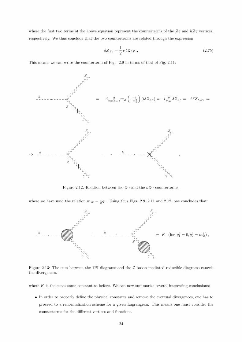
where the first two terms of the above equation represent the counterterms of the Zγ and hZγ vertices,
respectively. We thus conclude that the two counterterms are related through the expression
δZZγ =1
2v δZhZγ . (2.75)
This means we can write the counterterm of Fig. 2.9 in terms of that of Fig. 2.11:
h
Z
γ
Z
= i gcos(θW )mZ
(−i−m2
Z
)(iδZZγ) = −i g
mWδZZγ = −i δZhZγ ⇔
⇔ h
Z
γ
Z
= -h
Z
γ
,
Figure 2.12: Relation between the Zγ and the hZγ counterterms.
where we have used the relation mW = 12gv. Using thus Figs. 2.9, 2.11 and 2.12, one concludes that:
h
Z
γ
+h
Z
γ
Z
= K(for q2
1 = 0, q22 = m2
Z
),
Figure 2.13: The sum between the 1PI diagrams and the Z boson mediated reducible diagrams cancelsthe divergences.
where K is the exact same constant as before. We can now summarize several interesting conclusions:
• In order to properly define the physical constants and remove the eventual divergences, one has to
proceed to a renormalization scheme for a given Lagrangean. This means one must consider the
counterterms for the different vertices and functions.
24

• In a theory with spontaneous symmetry breaking, one can have counterterms for vertices which do
not exist at tree level, due to the mixing of the gauge fields. In particular, there exists a counterterm
for the hZγ vertex in the Standard Model.
• Although one can consider the reducible diagrams containing self-energies in the γ leg, the renor-
malization scheme obliges one to add their respective counterterms, in which case their contribution
is null - as can be seen from Figs. 2.8 and 2.10. Due to a relation between the Zγ and the hZγ
counterterms, the diagrams mediated by an internal Z boson are equal to the counterterm for the
1PI diagrams, which means that one can use the former instead of the latter, with the advantage
that no counterterms are explicitly necessary.
• From the full set of reducible diagrams13, we have only considered the ones mediated by an internal
Z boson, since the others are null. It should be emphasized, though, that no reducible diagrams
were needed at all, as it is patent in Figs. 2.8 and 2.11. In fact, from Eqs. 2.73 and 2.74, one can
compute the value of δZhZγ - which is precisely14 that of Eq. 2.69.
13The full set consists of the diagrams with an internal Z propagator - first term of Fig. 2.9 - and diagrams with aninternal G0 propagator - middle term of Fig. 2.10.
14Apart form an irrelevant ε1.ε2 factor.
25

Chapter 3
The (CP conserving) 2HDM
3.1 The Model
We start with the CP conserving 2HDM, which is simpler (although less general) than the C2HDM.
One says that there is (explicit) CP violation when the potential has (explicit) complex parameters1, so
that a CP conserving model is one whose potential is exclusively composed of real parameters.
Keeping that in mind, our objective is to build a model which can describe correctly what we know
about particle physics today and which has the exact same physical content of the SM except in the scalar
sector - instead of just one Higgs doublet (Φ), we now consider two: Φ1 and Φ2, where both doublets are
taken to have the same electroweak quantum numbers as Φ. We should then ask what is going to change
with this addition.
First of all, the potential changes: it loses the form in Eq. 2.9. With two doublets Φ1 and Φ2,
the most general potential obeying the requirements of hermiticity, SU(2) × U(1) gauge symmetry and
renormalizability2 is
V = m211Φ†1Φ1 +m2
22Φ†2Φ2 −(m2
12Φ†1Φ2 + h.c.)
+λ1
2
(Φ†1Φ1
)2
+λ2
2
(Φ†2Φ2
)2
+ λ3Φ†1Φ1Φ†2Φ2
+ λ4Φ†1Φ2Φ†2Φ1 +
λ5
2
(Φ†1Φ2
)2
+[λ6Φ†1Φ1 + λ7Φ†2Φ2
]Φ†1Φ2 + h.c.
,
(3.1)
where m211, m2
22 and λ1→4 are real parameters, while m211 and λ5→7 are in general complex3.
It turns out that Eq. 3.1 leads to Flavour Changing Neutral Currents (FCNC)4. It is well known that
these FCNC are strongly suppressed by experimental results, so that one must find a way to avoid them.
Glashow, Weinberg and Paschos put forward a theorem [40] which proves that one simple way to avoid
those undesired currents is to impose that all fermions of the same electric charge can only couple to a
single Higgs doublet. One reasonable way to do this is to enforce the Z2 symmetry on the potential5,
1The potential is said to have explicit complex parameters when there is no basis for the fields in which all the parametersare real; see Appendix A.1.
2Hermiticity requires that, for each term A in the potential, we either have A†A or A + A†; invariance under SU(2)implies that every term must be a singlet (i.e., a scalar, a number) in the SU(2) space (therefore, only an even numberof fields is permitted in each term); invariance under U(1) requires that each term has null hypercharge (which is, in thissituation, always the case, since the the two doublets have the same hypercharge); finally, renormalizability requires thateach term has no more than 4 fields.
3See Appendix A.1.4In fact, it is the interaction between the fermions and the Higgs doublets which leads to FCNC. See Appendix A.4.5See Appendices A.3 and A.4.
26

which means that we only keep the terms in Eq. 3.1 which stay invariant under the transformation
Φ1 → −Φ1, Φ2 → Φ2, (3.2)
in which case the potential would reduce to
V = m211Φ†1Φ1+m2
22Φ†2Φ2 +λ1
2
(Φ†1Φ1
)2
+λ2
2
(Φ†2Φ2
)2
+ λ3Φ†1Φ1Φ†2Φ2
+ λ4Φ†1Φ2Φ†2Φ1 +
[λ5
2
(Φ†1Φ2
)2
+ h.c.
].
(3.3)
It is shown in Appendix A.1 that we can take λ5 real by rephasing Φ1 and Φ2, so that all the parameters
in Eq. 3.3 can be taken real, making the model a CP conserving one6. Eq. 3.3 is not, however, our final
expression for the potential; in fact, one generally includes a quadratic term (which violates softly the Z2
symmetry) since it does not lead to FCNC7 (which was what we were trying to avoid in the first place).
Our final expression for the potential is thus
V = m211Φ†1Φ1 +m2
22Φ†2Φ2 −m212
(Φ†1Φ2 + Φ†2Φ1
)+λ1
2
(Φ†1Φ1
)2
+λ2
2
(Φ†2Φ2
)2
+ λ3Φ†1Φ1Φ†2Φ2 + λ4Φ†1Φ2Φ†2Φ1 +λ5
2
[(Φ†1Φ2
)2
+(
Φ†2Φ1
)2],
(3.4)
where we are taking m212 to be real (although it can in general be complex), since we are interested in
a CP conserving model. We shall see in Section 3.2 that the parameters of Eq. 3.4 must obey several
requirements. Whenever we refer to the potential from now on, we refer to Eq. 3.4.
Besides the potential, other terms are changed due to the addition of a second scalar doublet. Before
we study them, though, let us focus on the two doublets. After the spontaneous symmetry breaking,
these can be parametrized as:
Φ1 =
φ+1
v1 + ρ1 + iη1√2
, Φ2 =
φ+2
v2 + ρ2 + iη2√2
, (3.5)
where φ+i , ρi and ηi, are real fields, and we are assuming that there is no CP violation in the vevs - v1
and v2 - so that these can be taken real and non-negative. We are using the convention v =√v2
1 + v22 =
(√
2GF )−1/2
= 246 GeV. Each one of the two components of each doublet is complex, which corresponds
to two real degrees of freedom. Hence, the set of the two doublets has 8 real degrees of freedom, which
means we are going to have 8 fields. When the SU(2) × U(1) electroweak symmetry is spontaneously
broken to U(1)EM , 3 of the fields become Goldstone bosons, G± and G0, which in turn are absorbed by
the physical bosons W± and Z in the unitary gauge. The remaining 5 degrees of freedom originate 5
Higgs fields. Three of these are electrically neutral, two of which are scalar (h and H) and the third one
is pseudoscalar (A)8; the remaining two bosons are electrically charged (H±). The latter are the new
charged particles which might contribute to the enhancement of the γγ channel events referred to in the
beginning of this thesis: we shall study its effect in the Zγ channel in Section 3.4.
For what follows, it is convenient to establish the basis change given by(H1
H2
)=
(cβ sβ
−sβ cβ
)(Φ1
Φ2
), (3.6)
6Please note that when talking about CP conservation, we always refer to the Higgs potential; we are assuming thatthere is CP violation in the Yukawa terms just like in the SM, leading to an irremovable complex phase in the CKM matrix.
7A quadratic term does not yield interactions, therefore, it cannot lead to FCNC.8This distinction between scalar and pseudoscalar can only be made in the context of a CP conserving model [41].
27
where cβ≡cos(β), sβ≡sin(β) and the β angle is defined in such a way that tanβ := v2/v1; this rotation
angle is going to be preponderant throughout the rest of this thesis. The H1 and H2 doublets can be
parametrized according to
H1 =
G+
v + hH1 + iG0√2
, H2 =
H+
hH2 + iA√2
, (3.7)
and they constitute the so called Higgs basis [42,43]. Using Eqs. 3.5 and 3.6, one can show that the vev
of H2 is zero while the one of H1 is v :=√v2
1 + v22 . One of the major advantages of the Higgs basis is
that the H1 doublet behaves just like the (only) SM doublet: acquires the vev and contains all the three
Goldstone bosons.
We are now interested in determining the physical states, this is, the states with well-defined mass.
In order to do so, one must expand the potential using Eq. 3.5 and keeping only the quadratic terms.
It is also necessary to consider the minimization equation: by definition, the vacuum corresponds to the
minimum of the potential, so that in the minimum - given by
< Φ1 >=
0v1√
2
, < Φ2 >=
0v2√
2
(3.8)
- one must have:
0 =∂V
∂Φ1
∣∣∣∣Φ1=<Φ1>
= 2m211v1 − 2m2
12v2 + λ1v31 + λ345v1v
22 ,
0 =∂V
∂Φ2
∣∣∣∣Φ2=<Φ2>
= 2m222v2 − 2m2
12v1 + λ2v32 + λ345v
21v2,
(3.9)
where λ345 = λ3 + λ4 + λ5. After some lengthy calculations, one concludes that both the Goldstone
bosons and the H± and A are already mass eigenstates: the former are massless, the latter have mass
given by
m2H± =
v21 + v2
2
2v1v2
[2m2
12 − v1v2 (λ4 + λ5)], m2
A =v2
1 + v22
2v1v2
(m2
12 − v1v2λ5
). (3.10)
The hH1 and hH2 fields are not yet mass eigenstates. In order to diagonalize their mass matrix, one
introduces the α angle (which shall also be present throughout this thesis), which is such that(H
h
)=
(cα sα
−sα cα
)(ρ1
ρ2
), (3.11)
where the new fields H and h are already the physical states. Using Eqs. 3.6 and 3.11, one can see that(H
h
)=
(cα−β sα−β
−sα−β cα−β
)(hH1
hH2
). (3.12)
The masses of these neutral states are
m2H,h =
1
2
[a+ d±
√(a− d)
2+ 4c2
], (3.13)
where
a =1
v1(m2
12v2 + v31λ1), c = [−m2
12 + v1v2(λ3 + λ4 + λ5)], d =1
v2(m2
12v1 + v32λ2). (3.14)
28

The 8 physical fields can be written in terms of the parametrization of Eq. 3.5 as:
H± =−sβφ±1 +cβφ±2 , G± = cβφ
±1 +sβφ
±2 ,
A = −sβη1+ cβη2, G0 = cβη1+ sβη2,
H = cαρ1+ sαρ2, h =−sαρ1+ cαρ2,
(3.15)
where cα ≡ cos(α), sα ≡ sin(α). We will assume hereafter the relation mh < mH . The parameters one
should use as input to the model are a question of choice; we shall use:
mh, mH , mA, mH± , sin(α), tan(β), m212, (3.16)
where the α and β angles are contained in the ranges [44]
−π2≤ α ≤ π
2, 0 ≤ β ≤ π
2. (3.17)
After this digression throughout the parametrizations and the physical fields, let us return to the
different parts of the Lagrangean which are changed in the 2HDM. The Yukawa sector is one of them:
the portion concerning quarks is no longer given by the two first terms of Eq. 2.12, but is instead
LYukawaquarks= −qL (Yd1Φ1 + Yd2Φ2)nR − qL
(Yu1Φ1 + Yu2Φ2
)pR + h.c., (3.18)
where Φj = iτ2Φ∗j and Yd1, Yd2, Yu1 and Yu2 are new 3 × 3 complex matrices composed of the Yukawa
couplings. We can now change to the Higgs basis and define new matrices Y Hd1 , Y Hd2 , Y Hu1 and Y Hu2 such
that:
LYukawaquarks= −qL
(Y Hd1H1 + Y Hd2H2
)nR − qL
(Y Hu1H1 + Y Hu2H2
)pR + h.c., (3.19)
where Hj = iτ2H∗j . The equivalence between Eqs. 3.18 and 3.19 can be shown using the relations(
Y Hd1
Y Hd1
)=
(cβ sβ
−sβ cβ
)(Yd1
Yd2
),
(Y Hu1
Y Hu1
)=
(cβ sβ
−sβ cβ
)(Yu1
Yu2
), (3.20)
as well as Eq. 3.6. We now change the quarks to the mass basis - just as we did in Eq. 2.20 - using new
matrices U , which are defined in order to diagonalize the H1 couplings:
NU1:= diag(mu,mc,mt) =
v√2U†uLY
Hu1UuR, ND1 := diag(md,ms,mb) =
v√2U†dLY
Hd1 UdR. (3.21)
In this case, however, the couplings with H2 become
NU2 :=v√2U†uLY
Hu2UuR, ND2 :=
v√2U†dLY
Hd2 UdR, (3.22)
and are not diagonal in general. Using an expression equivalent to 2.209, the Yukawa Lagrangean for the
quarks can thus be expressed as
LYukawaquarks= −√
2
v
[(uLV, dL
)(ND1
H1 +ND2H2) dR +
(uL, dLV
†) (NU1H1 +NU2
H2
)uR + h.c.
],
(3.23)
where V = U†uLUdL is the CKM matrix. I am using again a very compact notation: the vectorial products
in the above equation concern the SU(2) space.
9Remember that the U matrices are in general different from the SM ones.
29
Please note that Eq. 3.18 and the subsequent equations allow quarks to couple with both Higgs
doublets. However, as it is discussed in detail in Appendix A.4, this will lead to FCNC at tree level. As
we have mentioned, the usual method employed to avoid it is enforcing the Z2 symmetry to the fields.
This can, nevertheless, be made in multiple ways10. We shall study four models, known as Type I, Type
II, Lepton Specific and Flipped, which are described in Appendix A.3. The final Yukawa Lagrangean for
the quarks thus depends on the model.
We shall now turn our attention to the scalar kinetic term. In the SM, it was given by the first term
of Eq. 2.8. Now that we have a second doublet, it becomes11
LHiggskinetic=∣∣∣D(Φ1) Φ1
∣∣∣2 +∣∣∣D(Φ2) Φ2
∣∣∣2 =∣∣∣D(H1)H1
∣∣∣2 +∣∣∣D(H2)H2
∣∣∣2, (3.25)
where D(j) is given by the first expression of Eq. 2.7; the second equality is immediate given Eq. 3.6. As
aforementioned, a remarkable advantage of the Higgs basis is that the computations concerning H1 are
precisely the same as those concerning the SM doublet. Another major advantage in using this basis is
that, through comparison between Eqs. 2.15 and 3.7, one can clearly see that the expressions for the gauge
fixing and the ghosts terms in the 2HDM Lagrangean are precisely the same as the SM ones. This has
to do with the fact that there are the exact same 3 Goldstone bosons in both scenarios - which explains
the equality of the gauge fixing terms - and there are thus the very same gauge fields - which explains
the equality of the ghosts terms. Although these two pairs of expressions are identical, in the 2HDM one
has several extra fields which naturally change the SM Feynman vertices.
3.2 Constraints
As mentioned in the previous section, the parameters of the potential 3.4 are constrained by some
requirements. These are:
1. Minimum constraints: although Eq. 3.9 guarantees we are in a local extreme of the potential,
it does not demand that that extreme is a minimum. One should thus find some constraints which
assure one chooses the pair of values (〈Φ1〉, 〈Φ2〉) from all the (Φ1,Φ2) space such that V is in a
minimum situation: this corresponds to a positive 2nd derivative, which in this case means that the
Hessian matrix of Eq. 3.9 must be positive definite at the vacuum. This corresponds to all Higgs
masses (mh, mH , mA and mH±) being positive.
One could still ask how do we know that the minimum chosen corresponds to the global minimum,
and not just to a relative one. It has been shown in Ref. [45] that if the minimum violates electric
10For each field, one can choose whether it transforms into itself or into its symmetric under the Z2 symmetry; seeAppendix A.3.
11Please note that despite being consistent with the symmetry of the Lagrangean, the interference terms should not beadded; in fact, one would have
LHiggskinetic= |DΦ1|2 + |DΦ2|2 + (DΦ1)† (DΦ2) + (DΦ2)† (DΦ1)
=((DΦ1)† (DΦ2)†
) (1 11 1
)((DΦ1)
(DΦ2)
).
(3.24)
One can diagonalize this interference matrix and find the eigenvalues 0 and 2, the first of which would mean one wouldobtain a non-propagating field - but this has no physical meaning.
30
charge conservation (which would be devastating), then it is unique; if the model violates CP
conservation (which is not the case under consideration), then it is also unique. Only when there
is electric charge conservation and the model is a CP conserving one there is the chance of existing
two minima; in this case, the condition
m212
(m2
11 −√λ1
λ2m2
22
)(tanβ − 4
√λ1
λ2
)> 0 (3.26)
is a necessary and sufficient one for the minimum to be unique [46].
2. Positivity constraints: in order to have one minimum value, one must assure that the potential
is bounded from below (V > −∞) [47]. This corresponds to [48]:
λ1 > 0, λ2 > 0, λ3 > −√λ1λ2, λ3 + λ4 − |λ5| > −
√λ1λ2. (3.27)
3. Perturbative unitarity constraints: these constraints refer to the unitarity of the S-matrix12.
This unitarity puts bounds on the amplitude of partial waves [49–53], which in turn restrain the
values of the coupling constants. The requirement is such that the eigenvalues ΛZ2
Y σ of the high
energy Higgs-Higgs scattering matrix for the different initial state quantum numbers (hypercharge
Y , weak isospin σ and Z2 parity) obey the relation |ΛZ2
Y σ±| < 8π [54], where
Λeven21± =
1
2
(λ1 + λ2 ±
√(λ1 − λ2)
2+ 4|λ5|2
), Λodd
21 = λ3 + λ4, Λodd20 = λ3 − λ4,
Λeven01± =
1
2
(λ1 + λ2 ±
√(λ1 − λ2)
2+ 4λ2
4
), Λodd
01± = λ3 ± |λ5|,
Λeven00± =
1
2
(3(λ1 + λ2)±
√9(λ1 − λ2)
2+ 4(2λ3 + λ4)
2
), Λodd
00± = λ3 + 2λ4 ± 3|λ5|.
(3.28)
In models with spontaneous symmetry breaking, the couplings and the masses are related to each
other, which in practice means that the unitarity of the S-matrix implies upper bounds on masses
both in the SM as well as in the 2HDM [55]. It is therefore very useful to write the quartic couplings
of the potential in terms of the Higgs masses, the m212 term and the α and β angle [46]:
λ1 =1
v2c2β
(c2αm
2H + s2
αm2h −m2
12
sβcβ
),
λ2 =1
v2s2β
(s2αm
2H + c2αm
2h −m2
12
cβsβ
),
λ3 =2m2
H±
v2+s2α
(m2H −m2
h
)v2s2β
− m212
v2sβcβ,
λ4 =m2A − 2m2
H±
v2+
m212
v2sβcβ,
λ5 =m2
12
v2sβcβ− m2
A
v2.
(3.29)
4. Electroweak precision constraints: Peskin and Takeuchi [56, 57] have introduced the so called
oblique parameters S, T and U , which measure potential new physics in electroweak radiative
corrections. A reparametrization of this set of parameters also commonly used is the set ∆ρ,
12See, for example, Eq. 2.50 of Ref. [37].
31

∆κ and ∆r, which measure the radiative corrections to the total Z coupling strength, the effective
Weinberg angle and the W mass, respectively [58]. S, T , U are given in the 2HDM by the Eqs. (388),
(393) and (394) of Ref. [44]. In the CP-conserving case, the T matrix needed in Eq. (381) of the
same reference is the matrix which relates the fields from the Higgs basis with the physical states13:
hH1hH2A
= T
HhA
, (3.30)
where T can be obtained from Eqs. 3.5, 3.6 and 3.7:
T =
cα−β −sα−β 0
sα−β cα−β 0
0 0 1
, (3.31)
see Eq. 3.12. In our simulations, we included the correlation between S and T [59].
5. (mH± , tan(β)) plane: The ranges formH± and tanβ where chosen to comply with the constraints
from Z → bb, b → sγ, and other B-Physics results. The constraints are basically the same in the
complex and real 2HDM because the charged Higgs couplings to fermions coincide – see, for example,
appendix C of Ref. [60]. Z → bb implies tanβ & 1 while, in Type II and Flipped, b→ sγ excludes
values of mH± below 340 GeV, at the 95% confidence level, with only a very mild dependence on
tanβ [58, 61–63]. In Type I and Lepton Specific, tanβ & 1 still holds, but mH± can be as low as
∼ 90GeV, even after the LHC results on pp→ tt with decay into H+b [64,65]. The ranges we have
chosen for mH± and tanβ conform to rather conservative bounds from these and other B-Physics
experiments, and, for comparison purposes, were taken to coincide with the constraints in Ref. [24].
3.3 Simulation procedure and introduction of the analysis
In this section, I introduce the analyses of the subsequent studies, which include: the h → Zγ decay
in the 2HDM, the available parameter space in the 2HDM and the wrong-sign Yukawa coupling between
the h and a pair of bottom quarks. In order to do so, I establish the new notation and explain the fit
procedure we have carried out in order to generate the numerical results.
Let me begin with the notation. Recall the ratios of observed rates to SM expectations introduced in
Chapter 1, µf , with f being some final state. This is what we use to constrain the ratios between the
2HDM and SM rates
µf = RP RD RTW , (3.32)
where the sub-indices P , D, and TW stand for “production”, “decay”, and “total width”, respectively.
Here,
RP =σ2HDM(pp→ h)
σSM(pp→ h),
13We have chosen this order of the physical fields in order to guarantee detT = +1, as is required for the formulae inRef. [44].
32
RD =Γ2HDM[h→ f ]
ΓSM[h→ f ],
RTW =ΓSM[h→ all]
Γ2HDM[h→ all], (3.33)
where σ is the Higgs production mechanism, Γ[h → f ] the decay width into the final state f , and
Γ[h→ all] is the total Higgs decay width14.
We introduce the notation a, λ and C to represent the coupling of h to the fermions, the charged
Higgs bosons and the vectorial bosons, respectively, divided by the value of the SM. While the latter is
given by
C =ghV VgSMhV V
= sin(β − α), where V V = W+W− or ZZ∗, (3.35)
the former depends on the type of the model and on the type of fermion, as can be seen in Table 3.1,
where Up and Down stand for the up-type quarks (u, c and t) and the down-type quarks (d, s and b),
respectively.
Type I Type II Lepton Specific Flipped
Up cos(α)sin(β)
cos(α)sin(β)
cos(α)sin(β)
cos(α)sin(β)
Down cos(α)sin(β) − sin(α)
cos(β)cos(α)sin(β) − sin(α)
cos(β)
Charged Leptons cos(α)sin(β) − sin(α)
cos(β) − sin(α)cos(β)
cos(α)sin(β)
Table 3.1: Values of a =ghffgSMhff
for each model and for the different fermions.
The value of λ is obtained with the help of FeynRules [66,67] (see Appendix C), and it is given by:
λ =
(− 1
8 v2 c2β s2β
)((m2h − 2m2
H±
)cos(α− 3β) sin(2β) + cos(α+ β)
[ (3m2
h + 2m2H±
)sin(2β)− 8m2
12
]).
(3.36)
For the ensuing study of the wrong-sign Yukawa coupling, we shall concentrate mostly on the Type
II 2HDM. In fact, given the experimental lower bound on tanβ, the coupling to the up-type quarks in
Type I and Type II - as well as the coupling to the down-type quarks in Type I - cannot have the wrong
sign [24]. We will use the notation kU and kD for the values of a related to the up-type quarks and the
down-type quarks in Type II, respectively. From Table 3.1, we have:
kU :=gType IIhUU
gSMhUU
=cos (α)
sin (β), kD :=
gType IIhDD
gSMhDD
= − sin (α)
cos (β). (3.37)
Since, in the SM limit, kU = kD = 1, and given that Eq. 3.17 implies cos(β) > 0, then
sin(α) < 0 ⇒ kD > 0 ⇔ SM sign,
sin(α) > 0 ⇒ kD < 0 ⇔ sign opposite to that of the SM.
(3.38)
14The ratios have this form since one wants to evaluate the quocient - between the model in consideration and the SM -of the quantity
σ(pp→ h) × BR(h→ f) = σ(pp→ h) ×Γ[h→ f ]
Γ[h→ all], (3.34)
where BR stands for the Branching Ratio.
33

Let us now focus on the implementation of the LHC constraints. We follow the strategy of Ref. [24],
and assume that all observed decays have been measured at the SM rates, i.e., with the (same) error 20%.
For the most part, we keep bb out of the mix for three reasons: it has larger errors (around 50%); it is
only measured in the V h production channel (recall Section 2.2); and, as we will show, it is not needed
in Type II models, where τ+τ− has the same effect (which, moreover, is not very large). We will only
assume that all production mechanisms are involved in bb and that its errors are of order 20% when we
wish to compare with Ref. [24], explaining the differences in production.
We have performed extensive simulations of the Type II 2HDM with the strategy commonly used in
literature: we set mh = 125 GeV and generate random points for:
α ∈[−π
2,π
2
], tanβ ∈ [1, 30] ,
mA ∈ [90, 900] GeV, mH ∈ [125, 900] GeV, mH± ∈ [340, 900] GeV, mA ∈[−9002, 9002
]GeV2.
These coincide with the ranges in Ref. [24], where tanβ and mH± were chosen to conform with the
contraints presented in the final of the last section.
For each point, we derive the parameters of the scalar potential using Eq. 3.29, and we keep only
those points which provide a bounded from below solution, respecting perturbative unitarity, and the
constraints from the oblique radiative parameters S, T, U . At the end of this procedure, we have a set of
possible 2HDM parameters, henceforth denoted simply by SET.
Next, we generate the rates for all channels, including all production mechanisms (recall Section 2.2):
gg → h (gluon fusion) at NNLO from HIGLU [28], bb → h at NNLO from SusHi [29], V h associated
production, tth, and V V → h (vector boson fusion) [30]. As we have seen, in the SM the production
cross section is dominated by the gluon fusion process with internal top quark. Generically speaking, this
also holds in the Type II 2HDM, but, given Eq. 3.37, the contribution from the gluon fusion process with
internal bottom quark becomes more important as tanβ increases.
3.4 The h→ Zγ decay in the 2HDM
Before entering the available parameter space in the model or the wrong-sign Yukawa coupling, we
study the h→ Zγ decay in the CP conserving 2HDM, where h is the lightest of the 3 neutral scalars and
has the same properties of the (single) Higgs boson from the SM. We want to compare this decay with
the one in the SM and understand what changes does the addition of a second Higgs doublet imply.
Let us begin with the Feynman diagrams. Besides those presented in Figs. 2.2 and 2.3, we now have
5 new diagrams due to the existence of a new charged scalar, H−, Fig. 3.1. The new diagrams are
h
γ
Z
E1
h
γ
Z
E1a
h
Z
E2γ
34

h
γ
E3
Z
Z
h
γ
E4
Z
Z
Figure 3.1: The new Feynman diagrams in the CP conserving 2HDM
equivalent to G8, G8a , G13, A1 and A6, but with the charged scalar instead of the charged Goldstone
boson. I call them E1, E1a , E2, E3 and E4, respectively. We write their amplitudes according to Section
2.3.2:
E1 = (i λ v)
(−i g cos 2θW
2 cos θW
)(−ie) i3 VSµ(−k + q1, k)VS
ν(−k + q1 + q2, k − q1) = E1a
E2 = (i λ v) i2(i e g
cos(2θW )
cos(θW )
)gµν
E3 =
(i
g
cos θWmZ
)(−i)
(−m2Z)
(i eg
cos 2θWcos θW
)gµνi = A1
E4 =
(i
g
cos θWmZ
)(−i)
(−m2Z)
(−i g cos 2θW
2 cos θW
)(−ie) i2 V νS (−k, k − q1)V µS (q1 − k, k) = A6
We see that E3 = A1 and E4 = A6, so that one can use Eq. 2.63 and Tables 2.1 and 2.2 to conclude that
the two reducible diagrams cancel each other exactly.
Let us now study the decay width. Instead of Eq. 2.49, we shall now have:
Γ =GFm
3h
4π√
2
α2
16π2
(1− m2
Z
m2h
)3
|aYF + CYG + λYH |2, (3.39)
where a is implicitly included in the fermionic sum and where the new function YH , relative to the charged
scalars, is given by
YH =− 1
tan(θW )
v2(1− tan2(θW )
)m2h −m2
Z
[m2Z
m2h −m2
Z
(B0
(m2h,m
2H± ,m
2H±
)−B0
(m2Z ,m
2H± ,m
2H±
))
+
(2m2
H±C0
(m2Z , 0,m
2h,m
2H± ,m
2H± ,m
2H±
)+ 1
)].
(3.40)
We present in Fig. 3.2 a scatterplot comparing the squared moduli of the different terms in Eq. 3.39,
where we are takingXW = C YG, Xt = kU YF top, Xb = kD YF bottom andXH± = λYH (we have considered
independently the top and bottom quarks contributions). The squared moduli have been computed in
the Type II 2HDM with both kD < 0 and kD > 0. We can distinguish the different orders of magnitude
of the terms: for sin(β−α) close to 1, we have that |XW |2 ∼ 102|Xt|2 ∼ 103|XH± |2 ∼ 105|Xb|2. Just like
in the SM, the diagrams mediated by internal vectorial bosons (G diagrams) have the most expressive
contribution. The charged Higgs contribution is non-negligible, being comparable to the top quark one.
We show on the left panel of Fig. 3.3 the interaction terms between XW , on the one hand, and Xt,
Xb and XH± , on the other. We are considering only the case kD > 0 for simplicity. We also present
the equivalent interactions in the h → γγ decay (right panel), for comparison. All the interferences are
35
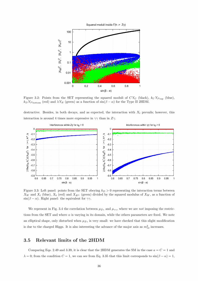
Figure 3.2: Points from the SET representing the squared moduli of C YG (black), kU YF top (blue),kD YF bottom (red) and λYH (green) as a function of sin(β − α) for the Type II 2HDM.
destructive. Besides, in both decays, and as expected, the interaction with Xt prevails; however, this
interaction is around 4 times more expressive in γγ than in Zγ.
Figure 3.3: Left panel: points from the SET obeying kD > 0 representing the interaction terms betweenXW and Xt (blue), Xb (red) and XH± (green) divided by the squared modulus of XW , as a function ofsin(β − α). Right panel: the equivalent for γγ.
We represent in Fig. 3.4 the correlation between µZγ and µγγ , where we are not imposing the restric-
tions from the SET and where α is varying in its domain, while the others parameters are fixed. We note
an elliptical shape, only disturbed when µZγ is very small: we have checked that this slight modification
is due to the charged Higgs. It is also interesting the advance of the major axis as m212 increases.
3.5 Relevant limits of the 2HDM
Comparing Eqs. 2.49 and 3.39, it is clear that the 2HDM generates the SM in the case a = C = 1 and
λ = 0; from the condition C = 1, we can see from Eq. 3.35 that this limit corresponds to sin(β − α) = 1,
36
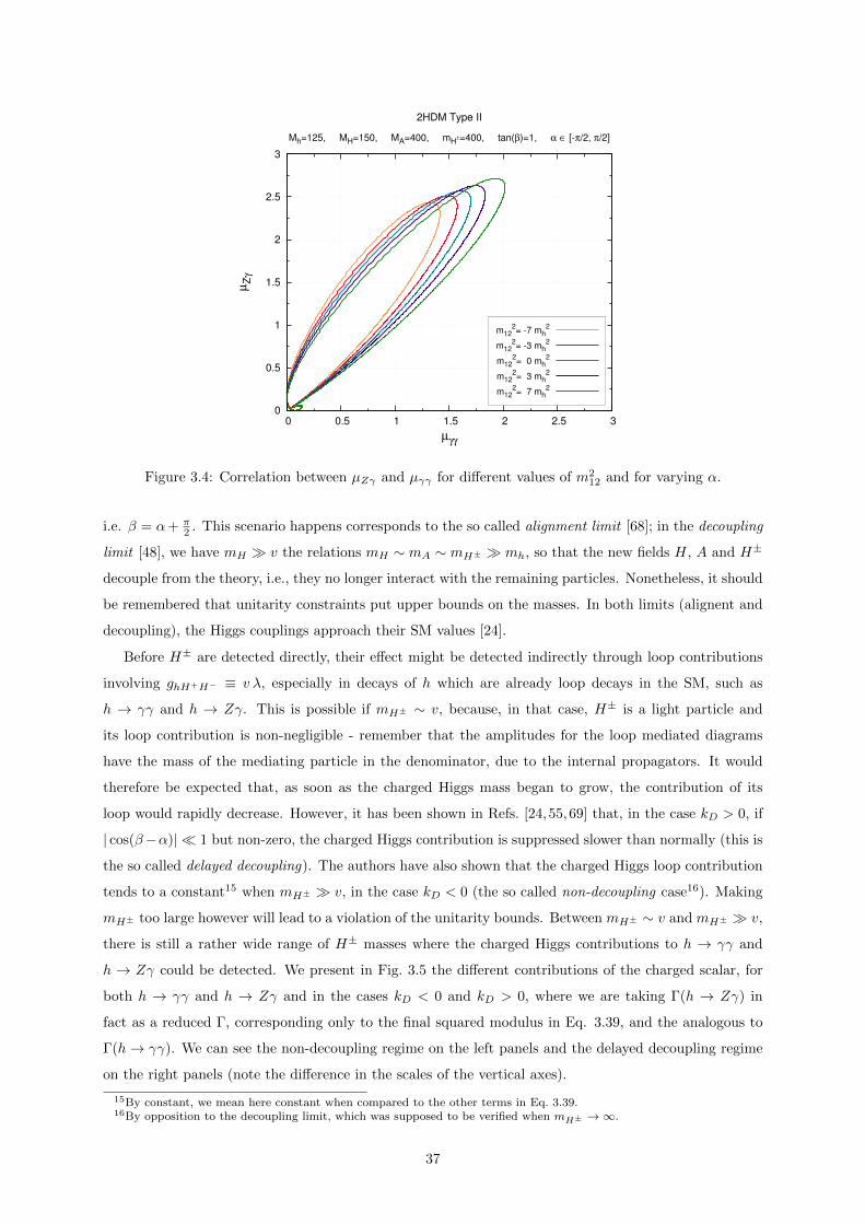
0
0.5
1
1.5
2
2.5
3
0 0.5 1 1.5 2 2.5 3
µZ
γ
µγγ
2HDM Type II
Mh=125, MH=150, MA=400, mH±=400, tan(β)=1, α ∈ [-π/2, π/2]
m122= -7 mh
2
m122= -3 mh
2
m122= 0 mh
2
m122= 3 mh
2
m122= 7 mh
2
Figure 3.4: Correlation between µZγ and µγγ for different values of m212 and for varying α.
i.e. β = α+ π2 . This scenario happens corresponds to the so called alignment limit [68]; in the decoupling
limit [48], we have mH v the relations mH ∼ mA ∼ mH± mh, so that the new fields H, A and H±
decouple from the theory, i.e., they no longer interact with the remaining particles. Nonetheless, it should
be remembered that unitarity constraints put upper bounds on the masses. In both limits (alignent and
decoupling), the Higgs couplings approach their SM values [24].
Before H± are detected directly, their effect might be detected indirectly through loop contributions
involving ghH+H− ≡ v λ, especially in decays of h which are already loop decays in the SM, such as
h → γγ and h → Zγ. This is possible if mH± ∼ v, because, in that case, H± is a light particle and
its loop contribution is non-negligible - remember that the amplitudes for the loop mediated diagrams
have the mass of the mediating particle in the denominator, due to the internal propagators. It would
therefore be expected that, as soon as the charged Higgs mass began to grow, the contribution of its
loop would rapidly decrease. However, it has been shown in Refs. [24, 55, 69] that, in the case kD > 0, if
| cos(β−α)| 1 but non-zero, the charged Higgs contribution is suppressed slower than normally (this is
the so called delayed decoupling). The authors have also shown that the charged Higgs loop contribution
tends to a constant15 when mH± v, in the case kD < 0 (the so called non-decoupling case16). Making
mH± too large however will lead to a violation of the unitarity bounds. Between mH± ∼ v and mH± v,
there is still a rather wide range of H± masses where the charged Higgs contributions to h → γγ and
h → Zγ could be detected. We present in Fig. 3.5 the different contributions of the charged scalar, for
both h → γγ and h → Zγ and in the cases kD < 0 and kD > 0, where we are taking Γ(h → Zγ) in
fact as a reduced Γ, corresponding only to the final squared modulus in Eq. 3.39, and the analogous to
Γ(h→ γγ). We can see the non-decoupling regime on the left panels and the delayed decoupling regime
on the right panels (note the difference in the scales of the vertical axes).
15By constant, we mean here constant when compared to the other terms in Eq. 3.39.16By opposition to the decoupling limit, which was supposed to be verified when mH± →∞.
37

Figure 3.5: Points from the SET representing the contribution of the charged scalar (with XH± = λYH)both in the Zγ and γγ channels, for kD < 0 and kD > 0, as a function of the charged scalar mass.
3.6 The parameter space and the wrong-sign Yukawa
3.6.1 Comparing with previous results
For this study, we start by requiring that all points in the SET obey kD < 0 and 0.8 ≤ µf ≤ 1.2
for the V V , τ+τ−, bb, and γγ at 8 GeV. The surviving points are plotted as a function of tanβ on the
left panel of Fig. 3.6, where we show the possible values of µγγ (in black) and µbb (in red/dark-gray).
We notice that, although µbb is in general larger than µγγ , the two regions overlap and, at the level of
deviations of 20% from the SM, both are compatible with the SM value of one. We now assume that
h→ V V is measured within 5% of the SM: 0.95 ≤ µV V ≤ 1.05. The result is plotted on the right panel
of Fig 3.6. We found that µγγ agrees, within errors, with that shown in Fig. 5-Left of Ref. [24], while our
result for µbb is well above theirs, which we also show in Fig. 3.6 (in cyan/light-gray). This is puzzling,
since we can reproduce their remaining plots.
After comparing notes with R. Santos from Ref. [24], we found that the difference originates in the
gluon fusion production rates, because we are using values from an more recent version of HIGLU [28],
and, eventually, different PDF’s and energy scales. For example, they quote
σ(gg → h)2HDMNNLO
σ(gg → hSM)NNLO= 1.06 [sin (β + α) = 1], (3.41)
38
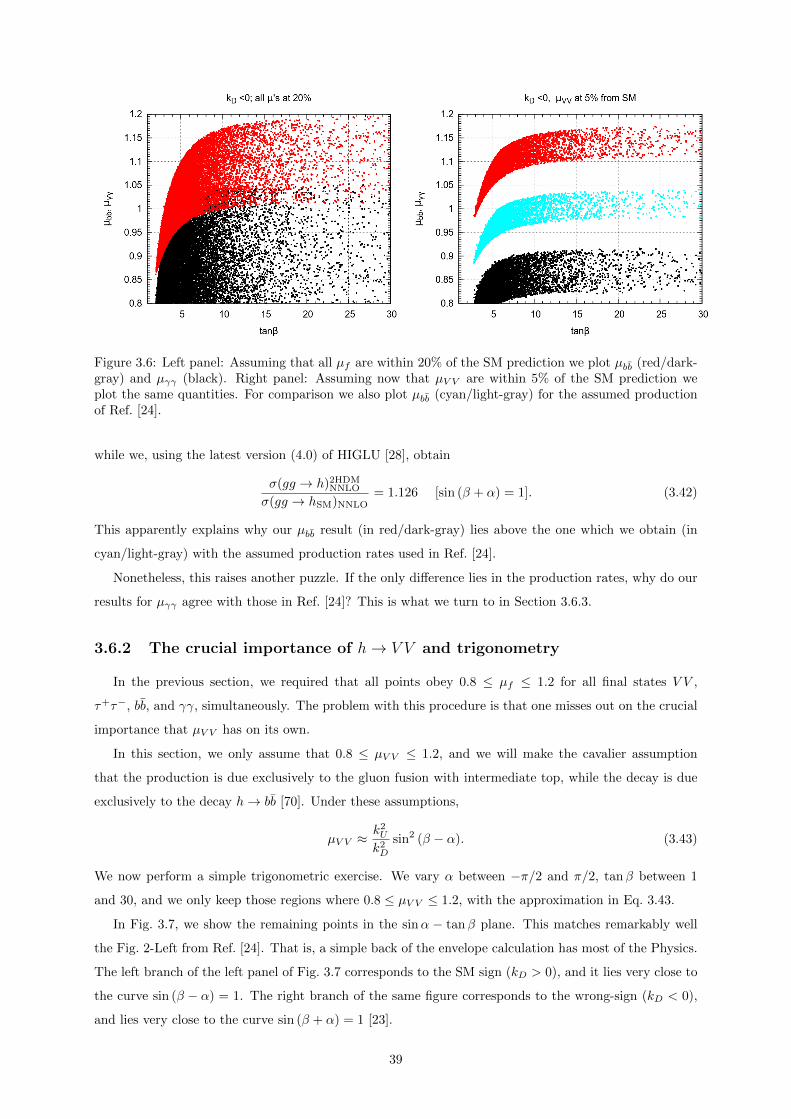
Figure 3.6: Left panel: Assuming that all µf are within 20% of the SM prediction we plot µbb (red/dark-gray) and µγγ (black). Right panel: Assuming now that µV V are within 5% of the SM prediction weplot the same quantities. For comparison we also plot µbb (cyan/light-gray) for the assumed productionof Ref. [24].
while we, using the latest version (4.0) of HIGLU [28], obtain
σ(gg → h)2HDMNNLO
σ(gg → hSM)NNLO= 1.126 [sin (β + α) = 1]. (3.42)
This apparently explains why our µbb result (in red/dark-gray) lies above the one which we obtain (in
cyan/light-gray) with the assumed production rates used in Ref. [24].
Nonetheless, this raises another puzzle. If the only difference lies in the production rates, why do our
results for µγγ agree with those in Ref. [24]? This is what we turn to in Section 3.6.3.
3.6.2 The crucial importance of h→ V V and trigonometry
In the previous section, we required that all points obey 0.8 ≤ µf ≤ 1.2 for all final states V V ,
τ+τ−, bb, and γγ, simultaneously. The problem with this procedure is that one misses out on the crucial
importance that µV V has on its own.
In this section, we only assume that 0.8 ≤ µV V ≤ 1.2, and we will make the cavalier assumption
that the production is due exclusively to the gluon fusion with intermediate top, while the decay is due
exclusively to the decay h→ bb [70]. Under these assumptions,
µV V ≈k2U
k2D
sin2 (β − α). (3.43)
We now perform a simple trigonometric exercise. We vary α between −π/2 and π/2, tanβ between 1
and 30, and we only keep those regions where 0.8 ≤ µV V ≤ 1.2, with the approximation in Eq. 3.43.
In Fig. 3.7, we show the remaining points in the sinα − tanβ plane. This matches remarkably well
the Fig. 2-Left from Ref. [24]. That is, a simple back of the envelope calculation has most of the Physics.
The left branch of the left panel of Fig. 3.7 corresponds to the SM sign (kD > 0), and it lies very close to
the curve sin (β − α) = 1. The right branch of the same figure corresponds to the wrong-sign (kD < 0),
and lies very close to the curve sin (β + α) = 1 [23].
39
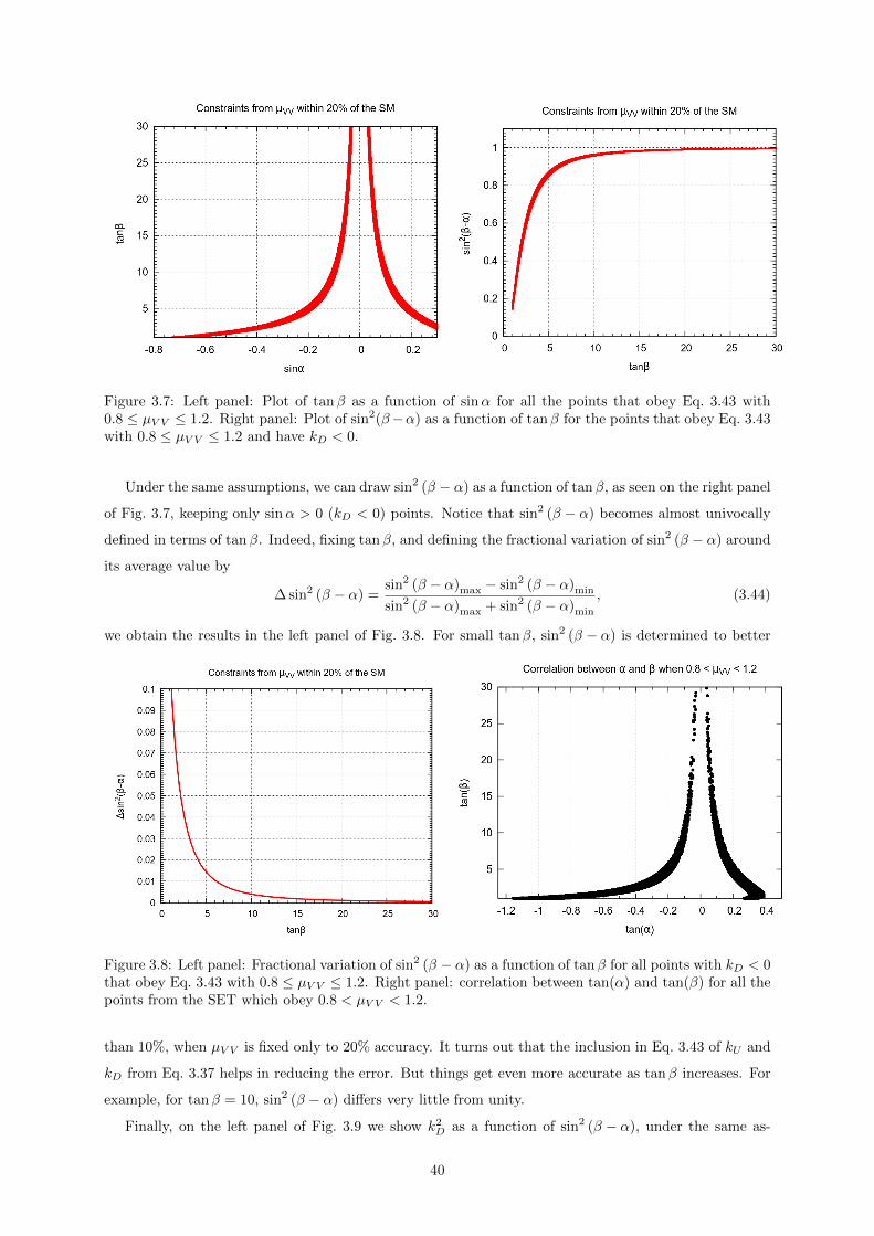
Figure 3.7: Left panel: Plot of tanβ as a function of sinα for all the points that obey Eq. 3.43 with0.8 ≤ µV V ≤ 1.2. Right panel: Plot of sin2(β−α) as a function of tanβ for the points that obey Eq. 3.43with 0.8 ≤ µV V ≤ 1.2 and have kD < 0.
Under the same assumptions, we can draw sin2 (β − α) as a function of tanβ, as seen on the right panel
of Fig. 3.7, keeping only sinα > 0 (kD < 0) points. Notice that sin2 (β − α) becomes almost univocally
defined in terms of tanβ. Indeed, fixing tanβ, and defining the fractional variation of sin2 (β − α) around
its average value by
∆ sin2 (β − α) =sin2 (β − α)max − sin2 (β − α)min
sin2 (β − α)max + sin2 (β − α)min
, (3.44)
we obtain the results in the left panel of Fig. 3.8. For small tanβ, sin2 (β − α) is determined to better
Figure 3.8: Left panel: Fractional variation of sin2 (β − α) as a function of tanβ for all points with kD < 0that obey Eq. 3.43 with 0.8 ≤ µV V ≤ 1.2. Right panel: correlation between tan(α) and tan(β) for all thepoints from the SET which obey 0.8 < µV V < 1.2.
than 10%, when µV V is fixed only to 20% accuracy. It turns out that the inclusion in Eq. 3.43 of kU and
kD from Eq. 3.37 helps in reducing the error. But things get even more accurate as tanβ increases. For
example, for tanβ = 10, sin2 (β − α) differs very little from unity.
Finally, on the left panel of Fig. 3.9 we show k2D as a function of sin2 (β − α), under the same as-
40
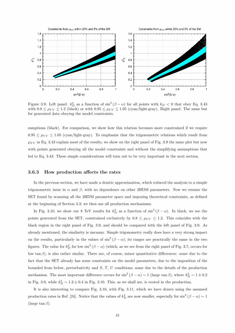
Figure 3.9: Left panel: k2D as a function of sin2 (β − α) for all points with kD < 0 that obey Eq. 3.43
with 0.8 ≤ µV V ≤ 1.2 (black) or with 0.95 ≤ µV V ≤ 1.05 (cyan/light-gray). Right panel: The same butfor generated data obeying the model constraints.
sumptions (black). For comparison, we show how this relation becomes more constrained if we require
0.95 ≤ µV V ≤ 1.05 (cyan/light-gray). To emphasize that the trigonometric relations which result from
µV V in Eq. 3.43 explain most of the results, we show on the right panel of Fig. 3.9 the same plot but now
with points generated obeying all the model constraints and without the simplifying assumptions that
led to Eq. 3.43. These simple considerations will turn out to be very important in the next section.
3.6.3 How production affects the rates
In the previous section, we have made a drastic approximation, which reduced the analysis to a simple
trigonometric issue in α and β, with no dependence on other 2HDM parameters. Now we resume the
SET found by scanning all the 2HDM parameter space and imposing theoretical constraints, as defined
at the beginning of Section 3.3; we then use all production mechanisms.
In Fig. 3.10, we show our 8 TeV results for k2D as a function of sin2 (β − α). In black, we see the
points generated from the SET, constrained exclusively by 0.8 ≤ µV V ≤ 1.2. This coincides with the
black region in the right panel of Fig. 3.9, and should be compared with the left panel of Fig. 3.9. As
already mentioned, the similarity is uncanny. Simple trigonometry really does have a very strong impact
on the results, particularly in the values of sin2 (β − α); its ranges are practically the same in the two
figures. The value for k2D for low sin2 (β − α) (which, as we see from the right panel of Fig. 3.7, occurs for
low tanβ), is also rather similar. There are, of course, minor quantitative differences: some due to the
fact that the SET already has some constraints on the model parameters, due to the imposition of the
bounded from below, perturbativity and S, T , U conditions; some due to the details of the production
mechanism. The most important difference occurs for sin2 (β − α) ∼ 1 (large tanβ), where k2D ∼ 1± 0.2
in Fig. 3.9, while k2D ∼ 1.2± 0.4 in Fig. 3.10. This, as we shall see, is rooted in the production.
It is also interesting to compare Fig. 3.10, with Fig. 3.11, which we have drawn using the assumed
production rates in Ref. [24]. Notice that the values of k2D are now smaller, especially for sin2 (β − α) ∼ 1
(large tanβ).
41
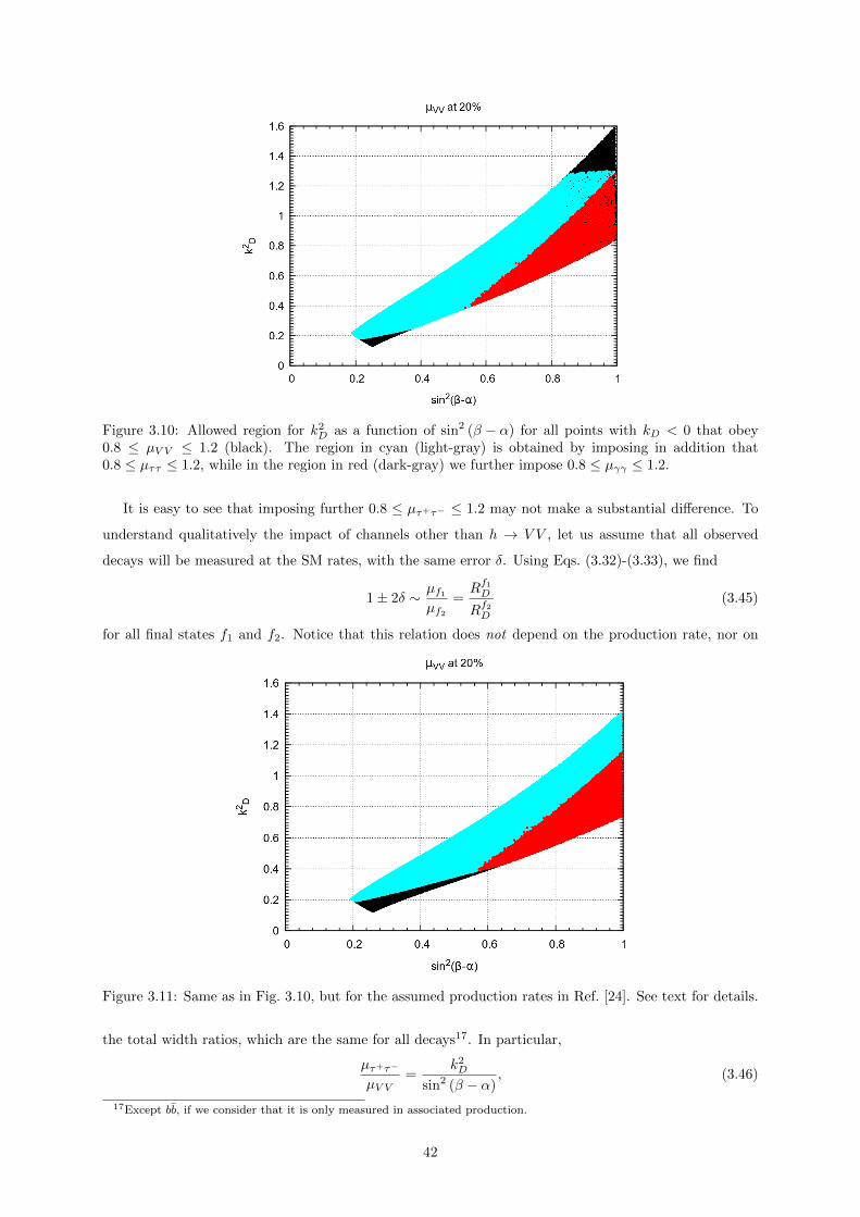
Figure 3.10: Allowed region for k2D as a function of sin2 (β − α) for all points with kD < 0 that obey
0.8 ≤ µV V ≤ 1.2 (black). The region in cyan (light-gray) is obtained by imposing in addition that0.8 ≤ µττ ≤ 1.2, while in the region in red (dark-gray) we further impose 0.8 ≤ µγγ ≤ 1.2.
It is easy to see that imposing further 0.8 ≤ µτ+τ− ≤ 1.2 may not make a substantial difference. To
understand qualitatively the impact of channels other than h → V V , let us assume that all observed
decays will be measured at the SM rates, with the same error δ. Using Eqs. (3.32)-(3.33), we find
1± 2δ ∼ µf1µf2
=Rf1DRf2D
(3.45)
for all final states f1 and f2. Notice that this relation does not depend on the production rate, nor on
Figure 3.11: Same as in Fig. 3.10, but for the assumed production rates in Ref. [24]. See text for details.
the total width ratios, which are the same for all decays17. In particular,
µτ+τ−
µV V=
k2D
sin2 (β − α), (3.46)
17Except bb, if we consider that it is only measured in associated production.
42
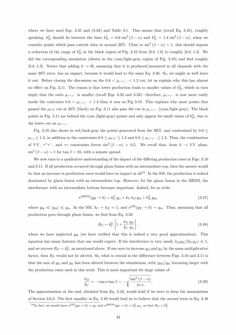
where we have used Eqs. 3.35 and (3.33) and Table 3.1. This means that (recall Eq. 3.45), roughly
speaking, k2D should lie between the lines k2
D = 0.6 sin2 (β − α) and k2D = 1.4 sin2 (β − α), when we
consider points which pass current data at around 20%. Close to sin2 (β − α) ∼ 1, this should impose
a reduction of the range of k2D in the black region of Fig. 3.10 from [0.8, 1.6] to roughly [0.8, 1.4]. We
did the corresponding simulation (shown in the cyan/light-gray region of Fig. 3.10) and find roughly
[0.8, 1.3]. Notice that adding h → bb, assuming that it is produced/measured in all channels with the
same 20% error, has no impact, because it would lead to the same Eq. 3.46. So, we might as well leave
it out. Before closing the discussion on the 0.8 < µτ+τ− < 1.2 cut, let us explain why this has almost
no effect on Fig. 3.11. The reason is that lower production leads to smaller values of k2D, which in turn
imply that the ratio µτ+τ− is smaller (recall Eqs. 3.32 and 3.33): therefore, µτ+τ− is now more easily
inside the contraints 0.8 < µτ+τ− < 1.2 than it was on Fig 3.10. This explains why most points that
passed the µV V cut at 20% (black) on Fig. 3.11 also pass the cut in µτ+τ− (cyan/light-gray). The black
points in Fig. 3.11 are behind the cyan (light-gray) points and only appear for small values of k2D, due to
the lower cut on µτ+τ− .
Fig. 3.10 also shows in red/dark-gray the points generated from the SET, and constrained by 0.8 ≤µγγ ≤ 1.2, in addition to the constraints 0.8 ≤ µV V ≤ 1.2 and 0.8 ≤ µτ+τ− ≤ 1.2. Thus, the combination
of V V , τ+τ−, and γγ constraints forces sin2 (β − α) > 0.5. We recall that, from h → V V alone,
sin2 (β − α) ∼ 1 for tanβ > 10, with a minute spread.
We now turn to a qualitative understanding of the impact of the differing production rates in Figs. 3.10
and 3.11. If all production occurred through gluon fusion with an intermediate top, then the answer would
be that an increase in production rates would have no impact at all18. In the SM, the production is indeed
dominated by gluon fusion with an intermediate top. However, for the gluon fusion in the 2HDM, the
interference with an intermediate bottom becomes important. Indeed, let us write
σ2HDM(gg → h) = k2U gtt + kU kD gtb + k2
D gbb, (3.47)
where gbb |gtb| gtt. In the SM, kU = kD = 1, and σSM(gg → h) ∼ gtt. Thus, assuming that all
production goes through gluon fusion, we find from Eq. 3.33
RP ∼ k2U
[1 +
kDkU
gtbgtt
]. (3.48)
where we have neglected gbb (we have verified that this is indeed a very good approximation). This
equation has many features that one would expect. If the interference is very small, kDgtb/(kUgtt) 1,
and we recoverRP ∼ k2U , as mentioned above. If one were to increase gtb and gtt by the same multiplicative
factor, then RP would not be altered. So, what is crucial in the difference between Figs. 3.10 and 3.11 is
that the mix of gtb and gtt has been altered between the simulations, with |gtb|/gtt becoming larger with
the production rates used in this work. This is more important for large values of
kDkU
= − tanα tanβ ∼ −√
sin2 (β − α)
µV V. (3.49)
The approximation at the end, obtained from Eq. 3.43, would hold if we were to keep the assumptions
of Section 3.6.2. The first equality in Eq. 3.49 would lead us to believe that the second term in Eq. 3.48
18In fact, we would have σSM(pp→ h) = gtt and σ2HDM(pp→ h) = k2U gtt, so that RP = k2
U .
43
is much more important as tanβ increases. However, this is mitigated by the fact that, as the analysis
in Section 3.6.2 and the approximation at the end of Eq. 3.49 show, kD/kU is tied to sin2 (β − α)/µV V ,
so that α and β are strongly correlated due to the requirement 0.8 < µV V < 1.2. This can be explicitly
seen on the right panel of Fig. 3.8.
Having established that RP is larger in our simulation than in the simulation of Fig. 3.11, we must
now understand its differing impact on µγγ , which is almost the same, and on µbb, which increases.
The crucial point comes from the previous section, where we found that 0.8 ≤ µV V ≤ 1.2 alone gives
a very tight constraint on the possible values of C2 = sin2 (β − α), for a given value of tanβ (recall the
left panel of Fig. 3.8). Thus, for fixed tanβ, if we wish to keep µV V = RP C2RTW constant and close to
one, we must always keep RPRTW ' constant. As a result, the only way to accommodate an increased
production is to have a decreased RTW - which is roughly determined by 1/k2D
19 - and therefore to
increase k2D. This explains why k2
D is larger when we use the larger production |gtb|/gtt, as in Fig. 3.10,
than it is when we use the smaller production |gtb|/gtt, as in Fig. 3.11. Since k2D appears in both h→ bb
and h → τ+τ− (this is, RDττ = RDbb = k2D), both are increased in our simulation, which therefore
implies that µττ and µbb are both increased in our simulation, i.e., both depend clearly on the production
rates.
If we were to take the right panel of Fig. 3.6 at face value, we might have been led to conclude that a
measurement 0.9 ≤ µbb ≤ 1.1 or 0.9 ≤ µτ+τ− ≤ 1.1 would already exclude the kD < 0 solution for large
tanβ, as can be seen in the right panel of Fig. 3.6 (red/dark-gray region). Unfortunately, as we have
shown, these rates are extremely sensitive to the production and, thus, cannot be used to exclude kD < 0
20.
In contrast, since the largest contribution to h→ γγ comes from the W boson diagrams, we then have
that RDγγ ' sin2 (β − α); but since this coupling is already fixed when one imposes µV V close to one,
this means that, for fixed tanβ, not only we have that RPRTW ' constant, but also RDγγ ' constant21.
Therefore, µγγ is constant as a whole, being thus rather insensitive to changes in the production, which
means it can be used to constrain kD < 0. As a result, our prediction for µγγ in the right panel of Fig. 3.6
mirrors that in Fig. 5-Left of Ref. [24].
The black points in the right panel of Fig. 3.6 represent the allowed region for µγγ when we take
0.95 ≤ µV V ≤ 1.05. As the highest value for this range is only slightly above 0.9, we agree with the
conclusion of Ref. [24] that a putative 5% measurement of h→ γγ at 8 TeV around the SM value would
rule out kD < 0.
In summary, the constraint RPRTW ' constant means that, when we increase the |gtb|/gtt mix in the
production rates, µγγ will stay the same22, as we have found in Fig. 3.6. In contrast, since an increased
production implies an increased k2D, we find that µbb = µτ+τ− = RP k
2DRTW ' constant k2
D must increase,
in accordance with what we see in the same figure.
There are three points to note. First, the next LHC run will occur at 14 TeV, while the current
19Since the bb is the main channel of decay.20Since the production functions values are always being updated.21So that, contrary to what happens in the µbb case, an increase in RP does not imply a change in RD.22And, indeed, µZγ .
44
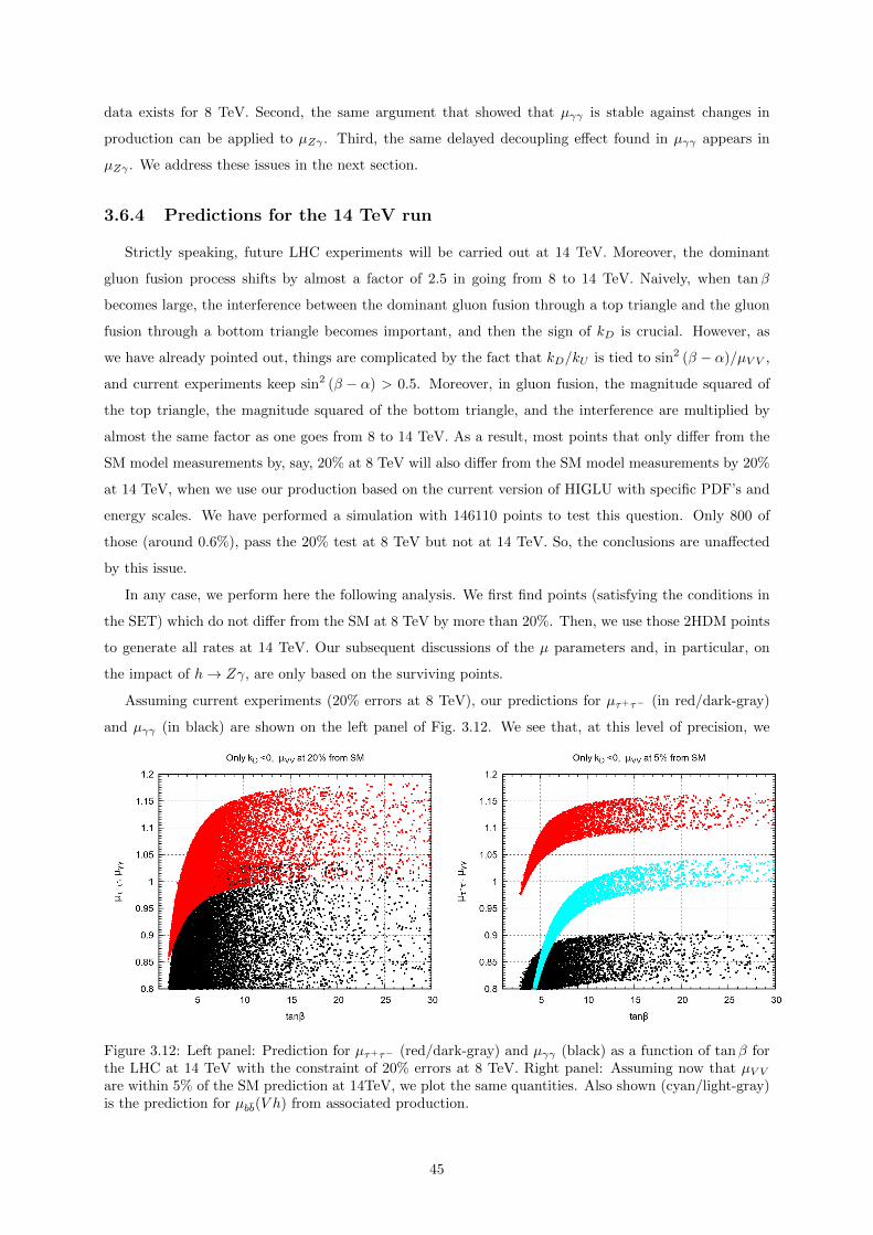
data exists for 8 TeV. Second, the same argument that showed that µγγ is stable against changes in
production can be applied to µZγ . Third, the same delayed decoupling effect found in µγγ appears in
µZγ . We address these issues in the next section.
3.6.4 Predictions for the 14 TeV run
Strictly speaking, future LHC experiments will be carried out at 14 TeV. Moreover, the dominant
gluon fusion process shifts by almost a factor of 2.5 in going from 8 to 14 TeV. Naively, when tanβ
becomes large, the interference between the dominant gluon fusion through a top triangle and the gluon
fusion through a bottom triangle becomes important, and then the sign of kD is crucial. However, as
we have already pointed out, things are complicated by the fact that kD/kU is tied to sin2 (β − α)/µV V ,
and current experiments keep sin2 (β − α) > 0.5. Moreover, in gluon fusion, the magnitude squared of
the top triangle, the magnitude squared of the bottom triangle, and the interference are multiplied by
almost the same factor as one goes from 8 to 14 TeV. As a result, most points that only differ from the
SM model measurements by, say, 20% at 8 TeV will also differ from the SM model measurements by 20%
at 14 TeV, when we use our production based on the current version of HIGLU with specific PDF’s and
energy scales. We have performed a simulation with 146110 points to test this question. Only 800 of
those (around 0.6%), pass the 20% test at 8 TeV but not at 14 TeV. So, the conclusions are unaffected
by this issue.
In any case, we perform here the following analysis. We first find points (satisfying the conditions in
the SET) which do not differ from the SM at 8 TeV by more than 20%. Then, we use those 2HDM points
to generate all rates at 14 TeV. Our subsequent discussions of the µ parameters and, in particular, on
the impact of h→ Zγ, are only based on the surviving points.
Assuming current experiments (20% errors at 8 TeV), our predictions for µτ+τ− (in red/dark-gray)
and µγγ (in black) are shown on the left panel of Fig. 3.12. We see that, at this level of precision, we
Figure 3.12: Left panel: Prediction for µτ+τ− (red/dark-gray) and µγγ (black) as a function of tanβ forthe LHC at 14 TeV with the constraint of 20% errors at 8 TeV. Right panel: Assuming now that µV Vare within 5% of the SM prediction at 14TeV, we plot the same quantities. Also shown (cyan/light-gray)is the prediction for µbb(V h) from associated production.
45

cannot rule out the kD < 0 branch.
If we now imagine that, in addition, the µV V are measured at 14 TeV to lie around unity with a 5%
precision, then we obtain for µτ+τ− (in red/dark-gray) and µγγ (in black) in the right panel of Fig. 3.12.
Here, we would be led to conclude that a 5% measurement of µτ+τ− ∼ 1 would exclude kD < 0 for large
tanβ. As explained in the previous section, this conclusion is misleading since the µτ+τ− (and the µbb
rates, combining all production modes) depend crucially on the detailed mix of the gluon production
through intermediate tops and bottoms. Thus, we agree with Ref. [24] that a 5% measurement of µγγ
can be used to exclude the wrong-sign solution, while µτ+τ− should not.
We recall that the µbb we present (in red/dark-gray) in Fig. 3.6 was calculated assuming that bb is
measured in all channels, and using our production rates. In that case, it would seem that a 5% of µbb
could exclude kD < 0. However, as with µτ+τ− , the result is very sensitive to the production, and, thus,
cannot be used to probe kD < 0. In foreseeing the 14 TeV run, we differ from Ref. [24], and study bb only
in the V h production channel, shown in cyan/light-gray on the right panel of Fig. 3.12. Unfortunately,
in contrast with what happens with our µbb in Fig. 3.6, a 5% measurement of µbb(V h) is centered around
unity for tanβ > 10, and, thus, it cannot be used to preclude kD < 0.
We now turn our attention to the decay h→ Zγ. As mentioned above, there are three good reasons
to look at this decay. First, the decay will be probed at LHC’s Run2, and there are already upper
bounds on it from Run1. Second, as for µγγ , we did not find a significant difference when using different
production rates. Third, the delayed decoupling that has been used in showing the usefulness of a future
measurement of µγγ is also present in µZγ .
Starting from the SET, we calculated µ for V V , γγ, and τ+τ− at 8 TeV, requiring that all lie within
20% of the SM. The remaining points were required to pass µV V , within 5% of the SM, at 14 TeV. We
then calculated µZγ , µτ+τ− and µγγ . Our results are shown in Fig. 3.13. There are bad news and good
Figure 3.13: Prediction for µτ+τ− (red/dark-gray), µZγ (cyan/light-gray) and µγγ (black) as a functionof tanβ, for the LHC at 14 TeV, with a measurement of µV V within 5% of the SM at 14 TeV.
46

news.
The bad news comes from the fact that the results in Fig. 3.13 show that µZγ . 1. Therefore, this
channel cannot be used to exclude the kD < 0 solution. The good news are the following. The ratio µV V ,
even at 20%, puts a strong bound on µZγ . In fact, we found that, for kD < 0 and before applying the µV V
constraint, µZγ could be as large as two for µγγ ∼ 1, as shown in the black region of Fig. 3.14. However,
Figure 3.14: Predictions for µZγ versus µγγ at 14 TeV, for kD < 0. In black, we have the points in theSET (obeying theoretical constraints and S, T, U , only). In red/dark-gray (cyan/light-gray), the pointssatisfying in addition V V within 20% (5%) of the SM, at 14 TeV.
the requirement that µV V should be within 20% of the SM drastically limits this upper bound, requiring
it to be very close to the SM value, as shown in the red/dark-gray region of Fig. 3.14. This means that
a measurement of & 1.3 in µZγ when 0.8 < µV V < 1.2 would exclude not only the SM but also the
CP conserving 2HDM. If we require a measurement of µV V to be within 5% of the SM (cyan/light-gray
region of Fig. 3.14), then both µγγ and µZγ have to be below their SM values for kD < 0. We find that
this effect is more predominant in γγ (µγγ < 0.9) than in Zγ (µZγ < 1).
Having discussed what we can learn from µγγ and µZγ for the wrong-sign branch, kD < 0, we can
ask what is the situation with the normal branch, kD > 0. This is shown in Fig. 3.15. We see that even
before requiring any constraint on µV V (black points), there is only a very small region with large µZγ
which is compatible with 0.8 ≤ µγγ ≤ 1.2 from current LHC data. In particular, points from the SET,
with µγγ ∼ 1 and µZγ ∼ 2, allowed for kD < 0 in the black region of Fig. 3.14, are almost forbidden for
kD > 0 in the black region of Fig. 3.15. If we further require µV V to be within 20% (red/dark-gray) or
5% (cyan/light-gray) both µγγ and µZγ have to be close to the SM values, with a wider range allowed
for µγγ .
We conclude that, for both signs of kD, current bounds on µV V already preclude a value of µZγ > 1.5
from being compatible with the usual 2HDM with softly broken Z2. A measurement in the next LHC run
of µV V lying within 5% of the SM will essentially force µZγ . 1 for kD < 0 and µZγ . 1.05 for kD > 0.
47
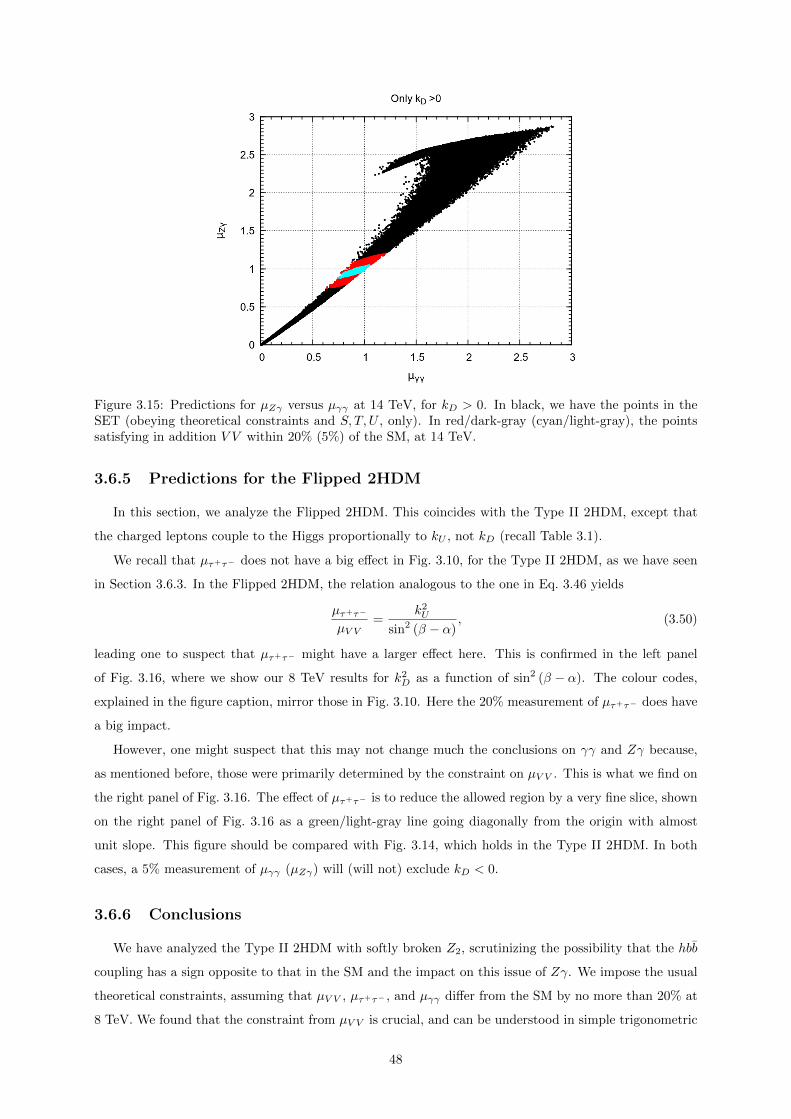
Figure 3.15: Predictions for µZγ versus µγγ at 14 TeV, for kD > 0. In black, we have the points in theSET (obeying theoretical constraints and S, T, U , only). In red/dark-gray (cyan/light-gray), the pointssatisfying in addition V V within 20% (5%) of the SM, at 14 TeV.
3.6.5 Predictions for the Flipped 2HDM
In this section, we analyze the Flipped 2HDM. This coincides with the Type II 2HDM, except that
the charged leptons couple to the Higgs proportionally to kU , not kD (recall Table 3.1).
We recall that µτ+τ− does not have a big effect in Fig. 3.10, for the Type II 2HDM, as we have seen
in Section 3.6.3. In the Flipped 2HDM, the relation analogous to the one in Eq. 3.46 yields
µτ+τ−
µV V=
k2U
sin2 (β − α), (3.50)
leading one to suspect that µτ+τ− might have a larger effect here. This is confirmed in the left panel
of Fig. 3.16, where we show our 8 TeV results for k2D as a function of sin2 (β − α). The colour codes,
explained in the figure caption, mirror those in Fig. 3.10. Here the 20% measurement of µτ+τ− does have
a big impact.
However, one might suspect that this may not change much the conclusions on γγ and Zγ because,
as mentioned before, those were primarily determined by the constraint on µV V . This is what we find on
the right panel of Fig. 3.16. The effect of µτ+τ− is to reduce the allowed region by a very fine slice, shown
on the right panel of Fig. 3.16 as a green/light-gray line going diagonally from the origin with almost
unit slope. This figure should be compared with Fig. 3.14, which holds in the Type II 2HDM. In both
cases, a 5% measurement of µγγ (µZγ) will (will not) exclude kD < 0.
3.6.6 Conclusions
We have analyzed the Type II 2HDM with softly broken Z2, scrutinizing the possibility that the hbb
coupling has a sign opposite to that in the SM and the impact on this issue of Zγ. We impose the usual
theoretical constraints, assuming that µV V , µτ+τ− , and µγγ differ from the SM by no more than 20% at
8 TeV. We found that the constraint from µV V is crucial, and can be understood in simple trigonometric
48
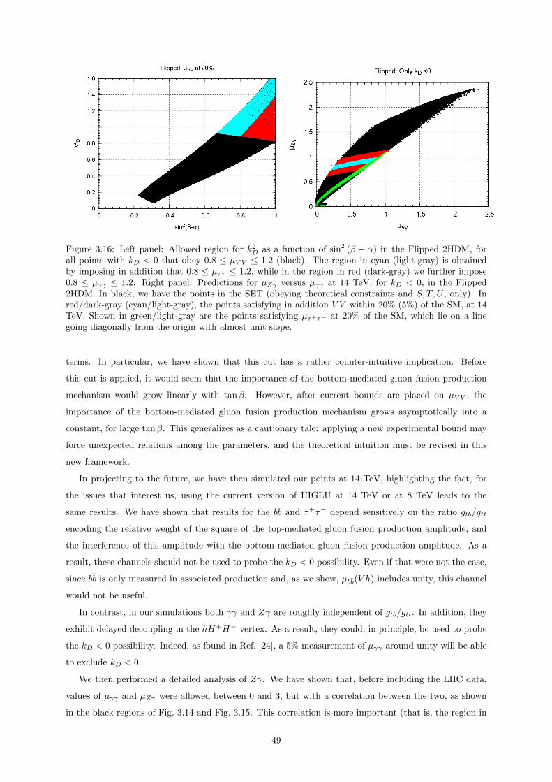
Figure 3.16: Left panel: Allowed region for k2D as a function of sin2 (β − α) in the Flipped 2HDM, for
all points with kD < 0 that obey 0.8 ≤ µV V ≤ 1.2 (black). The region in cyan (light-gray) is obtainedby imposing in addition that 0.8 ≤ µττ ≤ 1.2, while in the region in red (dark-gray) we further impose0.8 ≤ µγγ ≤ 1.2. Right panel: Predictions for µZγ versus µγγ at 14 TeV, for kD < 0, in the Flipped2HDM. In black, we have the points in the SET (obeying theoretical constraints and S, T, U , only). Inred/dark-gray (cyan/light-gray), the points satisfying in addition V V within 20% (5%) of the SM, at 14TeV. Shown in green/light-gray are the points satisfying µτ+τ− at 20% of the SM, which lie on a linegoing diagonally from the origin with almost unit slope.
terms. In particular, we have shown that this cut has a rather counter-intuitive implication. Before
this cut is applied, it would seem that the importance of the bottom-mediated gluon fusion production
mechanism would grow linearly with tanβ. However, after current bounds are placed on µV V , the
importance of the bottom-mediated gluon fusion production mechanism grows asymptotically into a
constant, for large tanβ. This generalizes as a cautionary tale: applying a new experimental bound may
force unexpected relations among the parameters, and the theoretical intuition must be revised in this
new framework.
In projecting to the future, we have then simulated our points at 14 TeV, highlighting the fact, for
the issues that interest us, using the current version of HIGLU at 14 TeV or at 8 TeV leads to the
same results. We have shown that results for the bb and τ+τ− depend sensitively on the ratio gtb/gtt
encoding the relative weight of the square of the top-mediated gluon fusion production amplitude, and
the interference of this amplitude with the bottom-mediated gluon fusion production amplitude. As a
result, these channels should not be used to probe the kD < 0 possibility. Even if that were not the case,
since bb is only measured in associated production and, as we show, µbb(V h) includes unity, this channel
would not be useful.
In contrast, in our simulations both γγ and Zγ are roughly independent of gtb/gtt. In addition, they
exhibit delayed decoupling in the hH+H− vertex. As a result, they could, in principle, be used to probe
the kD < 0 possibility. Indeed, as found in Ref. [24], a 5% measurement of µγγ around unity will be able
to exclude kD < 0.
We then performed a detailed analysis of Zγ. We have shown that, before including the LHC data,
values of µγγ and µZγ were allowed between 0 and 3, but with a correlation between the two, as shown
in the black regions of Fig. 3.14 and Fig. 3.15. This correlation is more important (that is, the region in
49

the figure is smaller) for kD > 0 than it is for kD < 0. In particular, µγγ ∼ 1 with µZγ ∼ 2 would be
possible in the latter case, but not in the former. Things change dramatically when the simple constraint
0.8 < µV V < 1.2 is imposed. In that case, we obtain the red/dark-gray regions of Fig. 3.14 (kD < 0) and
Fig. 3.15 (kD > 0). This already places µγγ and µZγ close to the SM, although, strictly speaking, points
with µγγ = 1 with µZγ = 1 are not allowed in our simulation when kD < 0. A 5% measurement of V V
around the SM at 14 TeV will bring µZγ closer to unity, for kD > 0, and just below unity, for kD < 0.
Thus, this decay cannot be used to exclude kD < 0.
But we have the reverse advantage. It is obvious that a measurement of µZγ > 1 would exclude the
SM. We have shown that a 5% precision on µV V around the SM, together with µZγ > 1, would also
exclude kD < 0, and, together with µZγ > 1.1, would exclude altogether the Type II 2HDM with softly
broken Z2. If µZγ turns out to lie a mere 20% above the SM value, then the softly broken Type II 2HDM
is not the solution.
Finally, we analyzed the Flipped 2HDM. Although there is a substantial difference in the k2D versus
sin2 (β − α) plane, this does not change dramatically the µγγ–µZγ correlation. As a result, here 5%
measurements of V V and γγ around the SM at 14 TeV will be enough to exclude kD < 0, while µZγ will
not.
50
Chapter 4
The C2HDM
4.1 The Model
The Complex 2HDM (C2HDM) is the most general case of the 2HDM with softly broken Z2 sym-
metry. Although the vast majority of the model is similar to the CP conserving case - discussed in the
previous chapter -, there are important differences. We shall thus present this new model mostly thorough
comparison with the previous one.
As it was mentioned in the beginning of Section 3.1, the C2HDM has explicit complex parameters in
the potential, which means that there is at least one complex phase in V which cannot be removed. This
implies that the potential loses its form of Eq. 3.4 and becomes
V = m211Φ†1Φ1 +m2
22Φ†2Φ2 −(m2
12Φ†1Φ2 + h.c.)
+λ1
2
(Φ†1Φ1
)2
+λ2
2
(Φ†2Φ2
)2
+ λ3Φ†1Φ1Φ†2Φ2 + λ4Φ†1Φ2Φ†2Φ1 +
[λ5
2
(Φ†1Φ2
)2
+ h.c.
],
(4.1)
where m212 and λ5 are in general complex. There is only CP violation if arg(λ5) 6= 2 arg(m2
12) (see
Appendix A.2).
We now have 3 minimization equations [14]:
m211 = −Re
(m2
12
) v2
v1+ λ1v
21 + λ345v
22 ,
m222 = −Re
(m2
12
) v1
v2+ λ2v
22 + λ345v
21 ,
Im(m2
12
)= v1 v2 Im(λ5),
(4.2)
where λ345 = λ3 +λ4 + Re(λ5). The first two equations are obtained in a analogous way to Eq. 3.9, while
the last one stems from the minimization of V with respect to arg(v2 − v1)1.
The parametrization of the doublets after the spontaneous symmetry breaking is slightly different
from that of the CP conserving case, Eq. 3.5. We shall use [60]:
Φ1 =
φ+1
v1 + η1 + iχ1√2
, Φ2 =
φ+2
v2 + η2 + iχ2√2
, (4.3)
1We rephase Φ1 and Φ2 in order to render the vev of Φ1 real, in which case v2 acquires a phase arg(v2 − v1); afterminimizing V with respect to this phase, we rephase Φ2 (see Appendix A.2) in order to render v2 real.
51
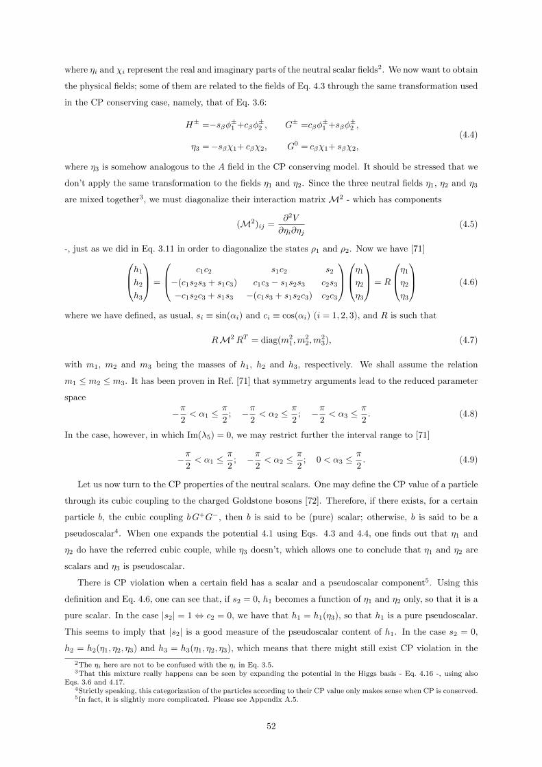
where ηi and χi represent the real and imaginary parts of the neutral scalar fields2. We now want to obtain
the physical fields; some of them are related to the fields of Eq. 4.3 through the same transformation used
in the CP conserving case, namely, that of Eq. 3.6:
H± =−sβφ±1 +cβφ±2 , G± =cβφ
±1 +sβφ
±2 ,
η3 =−sβχ1+ cβχ2, G0 = cβχ1+ sβχ2,
(4.4)
where η3 is somehow analogous to the A field in the CP conserving model. It should be stressed that we
don’t apply the same transformation to the fields η1 and η2. Since the three neutral fields η1, η2 and η3
are mixed together3, we must diagonalize their interaction matrix M2 - which has components
(M2)ij =∂2V
∂ηi∂ηj(4.5)
-, just as we did in Eq. 3.11 in order to diagonalize the states ρ1 and ρ2. Now we have [71]h1
h2
h3
=
c1c2 s1c2 s2
−(c1s2s3 + s1c3) c1c3 − s1s2s3 c2s3
−c1s2c3 + s1s3 −(c1s3 + s1s2c3) c2c3
η1
η2
η3
= R
η1
η2
η3
(4.6)
where we have defined, as usual, si ≡ sin(αi) and ci ≡ cos(αi) (i = 1, 2, 3), and R is such that
RM2RT = diag(m21,m
22,m
23), (4.7)
with m1, m2 and m3 being the masses of h1, h2 and h3, respectively. We shall assume the relation
m1 ≤ m2 ≤ m3. It has been proven in Ref. [71] that symmetry arguments lead to the reduced parameter
space
−π2< α1 ≤
π
2; −π
2< α2 ≤
π
2; −π
2< α3 ≤
π
2. (4.8)
In the case, however, in which Im(λ5) = 0, we may restrict further the interval range to [71]
−π2< α1 ≤
π
2; −π
2< α2 ≤
π
2; 0 < α3 ≤
π
2. (4.9)
Let us now turn to the CP properties of the neutral scalars. One may define the CP value of a particle
through its cubic coupling to the charged Goldstone bosons [72]. Therefore, if there exists, for a certain
particle b, the cubic coupling bG+G−, then b is said to be (pure) scalar; otherwise, b is said to be a
pseudoscalar4. When one expands the potential 4.1 using Eqs. 4.3 and 4.4, one finds out that η1 and
η2 do have the referred cubic couple, while η3 doesn’t, which allows one to conclude that η1 and η2 are
scalars and η3 is pseudoscalar.
There is CP violation when a certain field has a scalar and a pseudoscalar component5. Using this
definition and Eq. 4.6, one can see that, if s2 = 0, h1 becomes a function of η1 and η2 only, so that it is a
pure scalar. In the case |s2| = 1 ⇔ c2 = 0, we have that h1 = h1(η3), so that h1 is a pure pseudoscalar.
This seems to imply that |s2| is a good measure of the pseudoscalar content of h1. In the case s2 = 0,
h2 = h2(η1, η2, η3) and h3 = h3(η1, η2, η3), which means that there might still exist CP violation in the
2The ηi here are not to be confused with the ηi in Eq. 3.5.3That this mixture really happens can be seen by expanding the potential in the Higgs basis - Eq. 4.16 -, using also
Eqs. 3.6 and 4.17.4Strictly speaking, this categorization of the particles according to their CP value only makes sense when CP is conserved.5In fact, it is slightly more complicated. Please see Appendix A.5.
52

h2, h3 sector. In the case |s2| = 1 ⇔ c2 = 0, however, we have that h2 = h2(η1, η2) and h3 = h3(η1, η2)
(so that they are both pure scalars), whence we conclude that neither of the 3 physical fields has a
mixture between scalar and pseudoscalar components, which means that there is CP conservation. A
deeper analysis has been made in Refs. [71,73], where the authors have concluded that there are 2 other
limits of CP conservation, i.e., limits in which one of the neutral scalars is pseudoscalar, while the other
two are scalar. The three limits are:
α1 arbitrary, α2 = ±π2, α3 = arbitrary =⇒ h1 pseudoscalar,
α1 arbitrary, α2 = 0, α3 =π
2=⇒ h2 pseudoscalar,
α1 arbitrary, α2 = 0, α3 = 0 =⇒ h3 pseudoscalar.
(4.10)
These limits are represented on the (α2, α3) plane of Fig. 4.1.
- π/2
0
π/2
α3
- π/2 0 π/2
α2
h1 p
seud
oscalar
h1 p
seu
do
scal
ar
h2 pseudoscalar
h2 pseudoscalar
h3 pseudoscalar
Figure 4.1: Limits of CP conservation represented in the α2−α3 plan (reproduction of Fig. 1 of Ref. [60]).
Let us now focus on the input parameters of the model. We must first identify the number of inde-
pendent parameters of our potential. In Eq. 4.1, we have 12 real parameters: 8 real (v1, v2, m211, m2
22,
λ1→4) and 2 complex (m212 and λ5). Only 8 of them, though, are independent, since Eq. 4.2 provide 3
constraints and the relation v =√v2
1 + v22 = (
√2GF )
−1/2= 246 GeV provides the fourth. This means
that the set λ1,2,3,4, Re
(m2
12
), Im
(m2
12
), tan(β), Re(λ5)
(4.11)
describes a possible choice of input parameters for our model. However, it has been shown in Ref. [71]
that we can choose instead the set
m1, m2, mH± , α1, α2, α3, β, Re
(m2
12
), (4.12)
which we shall adopt henceforth. The value of m3 can be thus be calculated from this set [73]
m23 =
m21R13 [R12 tan(β)−R11] + m2
2R23 [R22 tan(β)−R21]
R33 [R31 −R32 tan(β)]. (4.13)
53

Of course, we are only interested in those cases where m23 > 0, and, due to our mass ordering, m2
3 >
m22 > m2
1. This places constraints on the relevant parameter space.
We now turn to the couplings of the lightest Higgs h1 to the fermions, the charged Higgs boson and
the vectorial bosons. As in the CP conserving 2HDM, we use the notation λ and C for the latter two,
respectively. The coupling to a pair of fermions, however, is now given by a + i b γ5, where a and b
represent the scalar and the pseudoscalar components of h1, respectively. In this new model, we have:
C = cβR11 + sβR12, (4.14)
where the entries of the matrix R are given in Eq. 4.6, and
−λ = cβ[s2βλ145 + c2βλ3
]R11 + sβ
[c2βλ245 + s2
βλ3
]R12 + sβcβ Im(λ5)R13, (4.15)
where λ145 = λ1 − λ4 − Re(λ5) and λ245 = λ2 − λ4 − Re(λ5). As in the 2HDM, the couplings to the
fermions depend on the specific model; they are presented in Table 4.1 in the form a+ i b γ5. Naturally,
making b = 0 and α2 = α3 = 0 will lead us to the CP conserving case, Table 3.1, with the equivalence
α = α1 − π2 .
Type I Type II Lepton Specific Flipped
Up R12
sβ− icβ R13
sβγ5
R12
sβ− icβ R13
sβγ5
R12
sβ− icβ R13
sβγ5
R12
sβ− icβ R13
sβγ5
Down R12
sβ+ icβ
R13
sβγ5
R11
cβ− isβ R13
cβγ5
R12
sβ+ icβ
R13
sβγ5
R11
cβ− isβ R13
cβγ5
Charged Leptons R12
sβ+ icβ
R13
sβγ5
R11
cβ− isβ R13
cβγ5
R11
cβ− isβ R13
cβγ5
R12
sβ+ icβ
R13
sβγ5
Table 4.1: Couplings of the fermions to the lightest scalar, h1, in the form a+ ibγ5.
4.2 Constraints
The constraints applicable to the C2HDM are similar to those in the CP conserving case, and have
been studied in Ref. [71]. We should note some differences, though. The T matrix, relevant for the
electroweak precision constraints, acquires a new form; in fact, and as we have seen above, we did not
apply the transformation 3.6 to the fields χ1 and χ2. If we did [42,43], we would obtain the relation 3.6,
with the Higgs basis given by
H1 =
G+
v +H0 + iG0√2
, H2 =
H+
R2 + iI2√2
. (4.16)
In this case, the relation between the η fields and the Higgs basis neutral fields is thusη1
η2
η3
=
cβ −sβ 0
sβ cβ 0
0 0 1
H0
R2
I2
= RH
H0
R2
I2
, (4.17)
which leads to the relation h1
h2
h3
= R
η1
η2
η3
= RRH
H0
R2
I2
. (4.18)
54
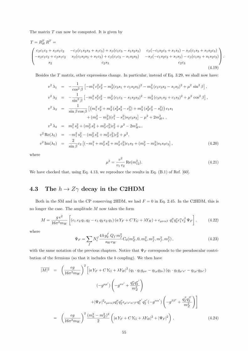
The matrix T can now be computed. It is given by
T = RTH RT = cβc1c2 + sβs1c2 −cβ(c1s2s3 + s1c3) + sβ(c1c3 − s1s2s3) cβ(−c1s2c3 + s1s3)− sβ(c1s3 + s1s2c3)
−sβc1c2 + cβs1c2 sβ(c1s2s3 + s1c3) + cβ(c1c3 − s1s2s3) −sβ(−c1s2c3 + s1s3)− cβ(c1s3 + s1s2c3)
s2 c2s3 c2c3
.
(4.19)
Besides the T matrix, other expressions change. In particular, instead of Eq. 3.29, we shall now have:
v2 λ1 = − 1
cos2 β
[−m2
1 c21c
22 −m2
2(c3s1 + c1s2s3)2 −m23 (c1c3s2 − s1s3)2 + µ2 sin2 β
],
v2 λ2 = − 1
sin2 β
[−m2
1 s21c
22 −m2
2 (c1c3 − s1s2s3)2 −m23 (c3s1s2 + c1s3)2 + µ2 cos2 β
],
v2 λ3 =1
sinβ cosβ
[(m2
1 c22 +m2
2 (s22s
23 − c23) +m2
3 (s22c
23 − s2
3))c1s1
+ (m23 −m2
2)(c21 − s21)s2c3s3
]− µ2 + 2m2
H± ,
v2 λ4 = m21 s
22 + (m2
2 s23 +m2
3 c23)c22 + µ2 − 2m2
H± ,
v2 Re(λ5) = −m21 s
22 − (m2
2 s23 +m2
3 c23)c22 + µ2,
v2 Im(λ5) =2
sinβc2[(−m2
1 +m22 s
23 +m2
3 c23)c1s2 + (m2
2 −m23)s1s3c3
], (4.20)
where
µ2 =v2
v1 v2Re(m2
12). (4.21)
We have checked that, using Eq. 4.13, we reproduce the results in Eq. (B.1) of Ref. [60].
4.3 The h→ Zγ decay in the C2HDM
Both in the SM and in the CP conserving 2HDM, we had F = 0 in Eq. 2.45. In the C2HDM, this is
no longer the case. The amplitude M now takes the form
M =g e2
16π2mW
[(ε1.ε2 q1.q2 − ε1.q2 ε2.q1) (a YF + C YG + λYH) + εµναβ q
µ1 qν2 εα1 εβ2 ΨF
], (4.22)
where
ΨF =∑f
Nfc
4 b gfV Qf m2f
sW cWC0(m2
Z , 0,m2h,m
2f ,m
2f ,m
2f ) , (4.23)
with the same notation of the previous chapters. Notice that ΨF corresponds to the pseudoscalar contri-
bution of the fermions (so that it includes the b coupling). We then have
|M |2 =
(eg
16π2mW
)2 [|a YF + C YG + λYH |2 (q1 · q1gµν − q1µq2ν) (q1 · q1gµ′ν′ − q1µ′q2ν′)
(−gµµ′)(−gνν′ +
qν2 qν′
2
m2Z
)
+|ΨF |2εµναβqµ1 qν2 εµ′ν′α′β′qµ′
1 qν′
2 (−gαα′)(−gββ′ +
qβ2 qβ′
2
m2Z
)]
=
(eg
16π2mW
)2(m2
h −m2Z)2
2
(|a YF + C YG + λYH |2 + |ΨF |2
), (4.24)
55

which in turn implies that the final decay width is given by
Γ(h→ Zγ) =GFα
2m3h
64√
2π3
(1− m2
Z
m2h
)3(|a YF + C YG + λYH |2 + |ΨF |2
). (4.25)
We present in Fig. 4.2 a scatterplot comparing the squared moduli of the different terms in Eq. 4.25, where
we are taking, just like in Section 3.4, XW = C YG, Xt = kU YF top, Xb = kD YF bottom and XH± = λYH6.
Once again, the squared moduli have been computed in the Type II 2HDM with both kD < 0 and
kD > 0. The new contributions, Ψt and Ψb, relative to the top and bottom quarks, respectively, give
a contribution of the order of that of Xt, thus being quite relevant. As in the SM and the 2HDM, the
diagrams mediated by internal vectorial bosons (G diagrams) have the most expressive contribution. This
Figure 4.2: Points obeying bounded from below, perturbative unitarity and S, T, U constraints represent-ing the squared moduli of C YG (black), kU YF top (blue), kD YF bottom (red), λYH (green), Ψt (purple)and Ψb (cyan) as a function of sin(β − (α1 − π/2)) for the Type II 2HDM.
figure should be compared with Fig. 3.2, which has roughly the same maximum values for a given value
of sin(β − α) as Fig. 4.2, although its range of allowed values is much narrower, since there are less
independent parameters in the real 2HDM than in the C2HDM (compare Eqs. 3.16 and 4.12), therefore
yielding a wider parameter space in the latter.
4.4 The parameter space and the wrong-sign Yukawa
For our procedure, we follow the strategy used in Section 3.3: we generate points in parameter space
with m1 = 125 GeV and with the new ranges
α1 ∈[−π
2,π
2
], α2 ∈
[−π
2,π
2
], α3 ∈
[0,π
2
], tanβ ∈ [1, 30] , m2 ∈ [125, 900] GeV,
mH± ∈ [340, 900] GeV (Type II and Flipped), mH± ∈ [100, 900] GeV (Type I and Lepton Specific),
m212 ∈
[−9002, 9002
]GeV2.
6Strictly speaking, in the C2HDM, kD and kU should be replaced with aD and aU : see Section 4.4.5.
56
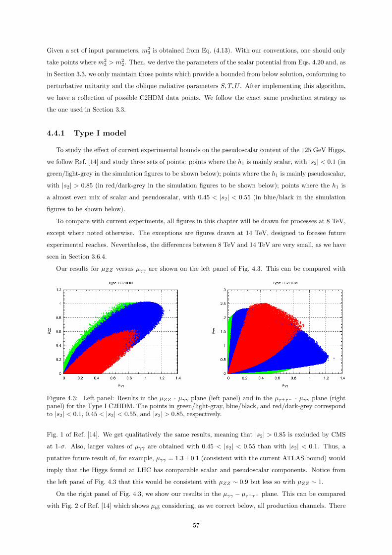
Given a set of input parameters, m23 is obtained from Eq. (4.13). With our conventions, one should only
take points where m23 > m2
2. Then, we derive the parameters of the scalar potential from Eqs. 4.20 and, as
in Section 3.3, we only maintain those points which provide a bounded from below solution, conforming to
perturbative unitarity and the oblique radiative parameters S, T, U . After implementing this algorithm,
we have a collection of possible C2HDM data points. We follow the exact same production strategy as
the one used in Section 3.3.
4.4.1 Type I model
To study the effect of current experimental bounds on the pseudoscalar content of the 125 GeV Higgs,
we follow Ref. [14] and study three sets of points: points where the h1 is mainly scalar, with |s2| < 0.1 (in
green/light-grey in the simulation figures to be shown below); points where the h1 is mainly pseudoscalar,
with |s2| > 0.85 (in red/dark-grey in the simulation figures to be shown below); points where the h1 is
a almost even mix of scalar and pseudoscalar, with 0.45 < |s2| < 0.55 (in blue/black in the simulation
figures to be shown below).
To compare with current experiments, all figures in this chapter will be drawn for processes at 8 TeV,
except where noted otherwise. The exceptions are figures drawn at 14 TeV, designed to foresee future
experimental reaches. Nevertheless, the differences between 8 TeV and 14 TeV are very small, as we have
seen in Section 3.6.4.
Our results for µZZ versus µγγ are shown on the left panel of Fig. 4.3. This can be compared with
Figure 4.3: Left panel: Results in the µZZ - µγγ plane (left panel) and in the µτ+τ− - µγγ plane (rightpanel) for the Type I C2HDM. The points in green/light-gray, blue/black, and red/dark-grey correspondto |s2| < 0.1, 0.45 < |s2| < 0.55, and |s2| > 0.85, respectively.
Fig. 1 of Ref. [14]. We get qualitatively the same results, meaning that |s2| > 0.85 is excluded by CMS
at 1-σ. Also, larger values of µγγ are obtained with 0.45 < |s2| < 0.55 than with |s2| < 0.1. Thus, a
putative future result of, for example, µγγ = 1.3± 0.1 (consistent with the current ATLAS bound) would
imply that the Higgs found at LHC has comparable scalar and pseudoscalar components. Notice from
the left panel of Fig. 4.3 that this would be consistent with µZZ ∼ 0.9 but less so with µZZ ∼ 1.
On the right panel of Fig. 4.3, we show our results in the µγγ − µτ+τ− plane. This can be compared
with Fig. 2 of Ref. [14] which shows µbb considering, as we correct below, all production channels. There
57

is qualitative agreement, but there are subtle differences, because we are using the latest version of
HIGLU [28], and, eventually, different PDF’s and energy scales. The difference is apparent when plotting
µτ+τ− as a function of tanβ. As we have seen in Section 3.6.3, µτ+τ− is very sensitive to the production
rates (and, thus, should be interpreted with care), while µγγ and µZγ are not. With this caution, we find
that values as large as µτ+τ− ∼ 2 are allowed. If one requires µγγ ∼ 1, then µτ+τ− lies roughly between
0.4 and 1.4.
In Ref. [14], µbb was calculated using all production channels. Here we use exclusively the V h pro-
duction mechanism that allows detection at LHC. Our results are shown on the left panel of Fig. 4.4. In
Figure 4.4: Results in the µbb(V h) - µγγ plane (left panel) and in the µZγ - µγγ plane (right panel) for theType I C2HDM. The points in green/light-gray, blue/black, and red/dark-grey correspond to |s2| < 0.1,0.45 < |s2| < 0.55, and |s2| > 0.85, respectively.
the Type I model, µbb(V h) . 1.1 for all values of |s2|, and µbb(V h) . 0.35 for |s2| > 0.85. Thus, we learn
that CMS excludes again |s2| > 0.85 at 1-σ (recall that even the SM ZZ and γγ are outside ATLAS’ 1-σ
intervals), and a good measurement of µbb(V h) will be useful in ruling out large pseudoscalar components.
Now we turn to central decay of this thesis. The right panel of Fig. 4.4 shows our results in the
µγγ − µZγ plane. We notice that large pseudoscalar components (large |s2|) imply small values for µZγ .
There are two points to stress. First, there is a strong correlation between µZγ and µγγ , even when all
values of s2 are taken into account. Second, that correlation is partly connected with s2. This can be
seen in the blue/black regions of Figs. 4.5, where we see that large values of µZγ and µγγ are only possible
around s2 ∼ 0 and h1 with a large scalar component. In contrast, a large pseudoscalar component implies
very small values for both µZγ and µγγ . As a result, a value of µZγ ∼ 1 would be very efficient in ruling
out a large pseudoscalar component. Figs. 4.5 also show in red/dark-grey (cyan/light-grey) the allowed
regions if we assume that the measurements of µV V at 14 TeV will center around unity with a 20% (5%)
error. The V V constraint implies that µγγ and µZγ are expected to lie close to their SM value in the
C2HDM and that |α2| should lie below 50 degrees. A similar analysis of the impact of V V , shows that
α3 can take any value and that |α1| should be larger than about 60 degrees.
4.4.2 Type II model
The results obtained in Type II for µZZ versus µγγ are shown on the left panel of Fig. 4.6. In
this model, values as large as µγγ ∼ 2.5 and µZZ ∼ 3 are allowed for small values of s2. In contrast,
58

Figure 4.5: Figures of µZγ (µγγ) on the left (right) panel, as a function of s2. The points in red/dark-grey(cyan/light-grey) were chosen to obey µV V = 1 within 20% (5%). These figures have been drawn for 14TeV.
|s2| > 0.85 forces both to be smaller than 0.8. This means that even the high central values quoted by
ATLAS are consistent with a Type II C2HDM where h1 has a dominant scalar component. In fact, one
can find s2 < 0.1 but also a few 0.45 < |s2| < 0.55 points within the ATLAS and CMS 1-σ bounds.
As occurred in Type I, both experiments exclude a large pseudoscalar component (|s2| > 0.85) at more
than 1-σ. However, in contrast to Type I, here the largest values of µγγ occur for s2 < 0.1 and not for
0.45 < |s2| < 0.55. That is, in Type I a large value (µγγ ∼ 1.2) favors a comparable scalar/pseudoscalar
mix, while in Type II a large value (here, µγγ ≥ 1.2) favors a pure scalar.
Figure 4.6: Results in the µZZ - µγγ plane (left panel) and in the µτ+τ− - µγγ plane (right panel) for theType II C2HDM. The points in green/light-gray, blue/black, and red/dark-grey correspond to |s2| < 0.1,0.45 < |s2| < 0.55, and |s2| > 0.85, respectively.
Curiously, the situation is the reverse when one considers µτ+τ− , which we show on the right panel of
Fig. 4.6. For example, for µγγ ∼ 1, a value of µτ+τ− ∼ 1.3 favors an even scalar/pseudoscalar mix over
the pure scalar solution. In contrast, |s2| is less easily constrained from µbb(V h), although µbb(V h) & 0.4
rules out |s2| > 0.85. Looking at the various channels, both CMS and ATLAS rule out |s2| > 0.85 by
more than 2-σ in Type II C2HDM. Better measurements of γγ, τ+τ−, and bb(V h) will be instrumental
in determining s2.
59

Next, we consider the simulations for Zγ, shown in on the left panel of Fig. 4.7. Large values for
Figure 4.7: Left panel: Type II results in the µZγ - µγγ plane. The points in red/dark-grey, blue/black,and green/light-gray correspond to |s2| < 0.1, 0.45 < |s2| < 0.55, and |s2| > 0.85, respectively. Rightpanel: Type II predictions in the µZγ - s2 plane. The points in red/dark-grey (cyan/light-grey) werechosen to obey µV V = 1 within 20% (5%). This figure has been draw at 14 TeV.
µZγ are possible for small |s2|. Comparing with the right panel of Fig. 4.4 we see that in Type II much
larger values of µZγ (and of µγγ) are allowed, but that there is still a strong correlation between the two
which, again, is partly due to s2. This is shown on the right panel of Fig. 4.7, where we see that large
values of µZγ require large values of µV V and correspond to an almost pure scalar. Measurements of µV V
within 20% of unity, force µZγ ∼ 1 and require |α2| . 50 degrees. This puts a further bound on a large
pseudoscalar component.
4.4.3 Lepton Specific model
In this case, the results for µZZ and µbb(V h) versus µγγ are very similar to those presented on the
left panels of Figs. 4.3 and 4.4 for Type I, respectively. The same holds for µZγ , shown on the right panel
of Fig. 4.4. Minute differences are as follows. Close to µγγ ∼ 1, one can get slightly larger values for
µZZ , up to approximately 1.1. Conversely, µγγ . 1.1 here, while µγγ . 1.3 in Type I. Here, as in Type
I, |s2| > 0.85 forces µbb(V h) < 0.3. Thus, a good measurement of µbb(V h) will be instrumental in ruling
out large pseudoscalar components.
As expected, the situation for µτ+τ− differs, as shown in Fig. 4.8. A large pseudoscalar component
(|s2| > 0.85) forces µτ+τ− > 1.2 when µγγ > 0.1. These values are ruled out by CMS at 1-σ. ATLAS, on
the other hand, is barely consistent with these values for µτ+τ− , but rules out this model (and the SM)
in µγγ at 1-σ.
4.4.4 Flipped model
The results for µγγ , µZZ , µbb(V h), and µZγ in this model, are similar to those for Type II. Slight
differences are as follows. Here µγγ (µZZ , µγγ ) can only be as large as 2.2 (2.5, 2.4), while one could
achieve 2.5 (2.9, 2.8) in Type II. The situation for µbb(V h) is virtually the same. In particular, |s2| > 0.85
is ruled out at 1-σ by both ATLAS and CMS.
60
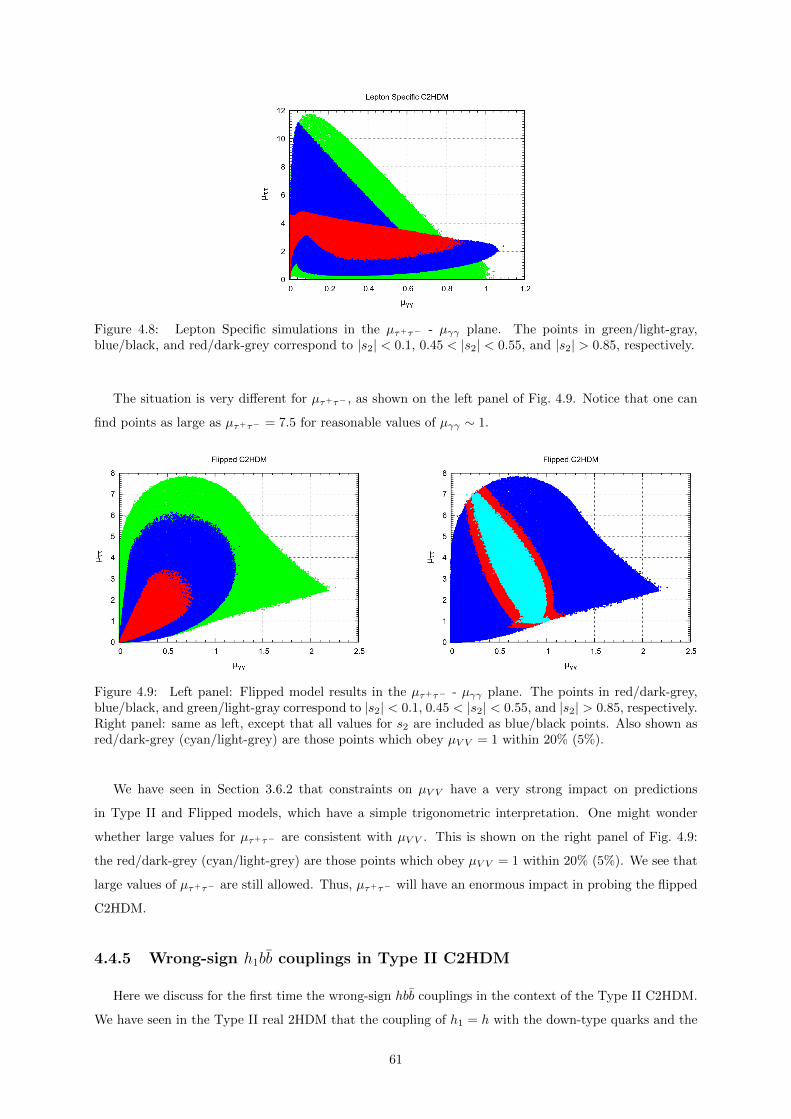
Figure 4.8: Lepton Specific simulations in the µτ+τ− - µγγ plane. The points in green/light-gray,blue/black, and red/dark-grey correspond to |s2| < 0.1, 0.45 < |s2| < 0.55, and |s2| > 0.85, respectively.
The situation is very different for µτ+τ− , as shown on the left panel of Fig. 4.9. Notice that one can
find points as large as µτ+τ− = 7.5 for reasonable values of µγγ ∼ 1.
Figure 4.9: Left panel: Flipped model results in the µτ+τ− - µγγ plane. The points in red/dark-grey,blue/black, and green/light-gray correspond to |s2| < 0.1, 0.45 < |s2| < 0.55, and |s2| > 0.85, respectively.Right panel: same as left, except that all values for s2 are included as blue/black points. Also shown asred/dark-grey (cyan/light-grey) are those points which obey µV V = 1 within 20% (5%).
We have seen in Section 3.6.2 that constraints on µV V have a very strong impact on predictions
in Type II and Flipped models, which have a simple trigonometric interpretation. One might wonder
whether large values for µτ+τ− are consistent with µV V . This is shown on the right panel of Fig. 4.9:
the red/dark-grey (cyan/light-grey) are those points which obey µV V = 1 within 20% (5%). We see that
large values of µτ+τ− are still allowed. Thus, µτ+τ− will have an enormous impact in probing the flipped
C2HDM.
4.4.5 Wrong-sign h1bb couplings in Type II C2HDM
Here we discuss for the first time the wrong-sign hbb couplings in the context of the Type II C2HDM.
We have seen in the Type II real 2HDM that the coupling of h1 = h with the down-type quarks and the
61
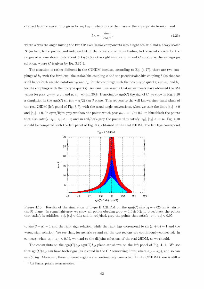
charged leptons was simply given by mfkD/v, where mf is the mass of the appropriate fermion, and
kD = − sinα
cosβ, (4.26)
where α was the angle mixing the two CP even scalar components into a light scalar h and a heavy scalar
H (in fact, to be precise and independent of the phase conventions leading to the usual choices for the
ranges of α, one should talk about C kD > 0 as the right sign solution and C kD < 0 as the wrong-sign
solution, where C is given by Eq. 3.357).
The situation is rather different in the C2HDM because, according to Eq. (4.27), there are two cou-
plings of h1 with the fermions: the scalar-like coupling a and the pseudoscalar-like coupling b (so that we
shall henceforth use the notation aD and bD for the couplings with the down-type quarks, and aU and bU
for the couplings with the up-type quarks). As usual, we assume that experiments have obtained the SM
values for µZZ , µWW , µγγ , and µτ+τ− within 20%. Denoting by sgn(C) the sign of C, we show in Fig. 4.10
a simulation in the sgn(C) sin (α1 − π/2)-tanβ plane. This reduces to the well known sinα-tanβ plane of
the real 2HDM (left panel of Fig. 3.7), with the usual angle conventions, when we take the limit |s2| → 0
and |s3| → 0. In cyan/light-grey we show the points which pass µV V = 1.0±0.2; in blue/black the points
that also satisfy |s2|, |s3| < 0.1; and in red/dark-grey the points that satisfy |s2|, |s3| < 0.05. Fig. 4.10
should be compared with the left panel of Fig. 3.7, obtained in the real 2HDM. The left legs correspond
Figure 4.10: Results of the simulation of Type II C2HDM on the sgn(C) sin (α1 − π/2)-tanβ (sinα-tanβ) plane. In cyan/light-grey we show all points obeying µV V = 1.0 ± 0.2; in blue/black the pointsthat satisfy in addition |s2|, |s3| < 0.1; and in red/dark-grey the points that satisfy |s2|, |s3| < 0.05.
to sin (β − α) ∼ 1 and the right sign solution, while the right legs correspond to sin (β + α) ∼ 1 and the
wrong-sign solution. We see that, for generic s2 and s3, the two regions are continuously connected. In
contrast, when |s2|, |s3| < 0.05, we tend to the disjoint solutions of the real 2HDM, as we should.
The constraints on the sgn(C) aD-sgn(C) bD plane are shown on the left panel of Fig. 4.11. We see
that sgn(C) aD can have both signs (as it could in the CP conserving limit, where aD = kD), and so can
sgn(C) bD. Moreover, these different regions are continuously connected. In the C2HDM there is still a
7Rui Santos, private communication.
62
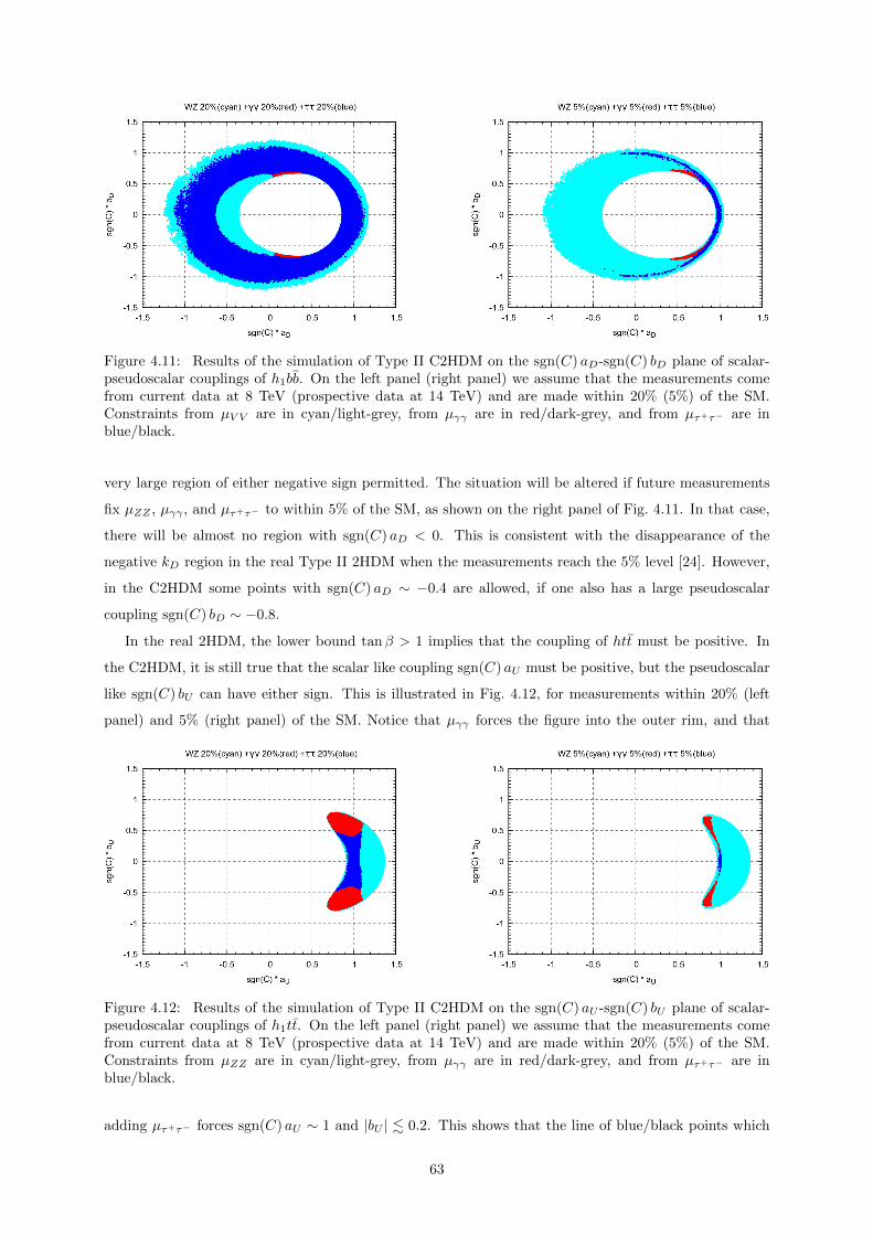
Figure 4.11: Results of the simulation of Type II C2HDM on the sgn(C) aD-sgn(C) bD plane of scalar-pseudoscalar couplings of h1bb. On the left panel (right panel) we assume that the measurements comefrom current data at 8 TeV (prospective data at 14 TeV) and are made within 20% (5%) of the SM.Constraints from µV V are in cyan/light-grey, from µγγ are in red/dark-grey, and from µτ+τ− are inblue/black.
very large region of either negative sign permitted. The situation will be altered if future measurements
fix µZZ , µγγ , and µτ+τ− to within 5% of the SM, as shown on the right panel of Fig. 4.11. In that case,
there will be almost no region with sgn(C) aD < 0. This is consistent with the disappearance of the
negative kD region in the real Type II 2HDM when the measurements reach the 5% level [24]. However,
in the C2HDM some points with sgn(C) aD ∼ −0.4 are allowed, if one also has a large pseudoscalar
coupling sgn(C) bD ∼ −0.8.
In the real 2HDM, the lower bound tanβ > 1 implies that the coupling of htt must be positive. In
the C2HDM, it is still true that the scalar like coupling sgn(C) aU must be positive, but the pseudoscalar
like sgn(C) bU can have either sign. This is illustrated in Fig. 4.12, for measurements within 20% (left
panel) and 5% (right panel) of the SM. Notice that µγγ forces the figure into the outer rim, and that
Figure 4.12: Results of the simulation of Type II C2HDM on the sgn(C) aU -sgn(C) bU plane of scalar-pseudoscalar couplings of h1tt. On the left panel (right panel) we assume that the measurements comefrom current data at 8 TeV (prospective data at 14 TeV) and are made within 20% (5%) of the SM.Constraints from µZZ are in cyan/light-grey, from µγγ are in red/dark-grey, and from µτ+τ− are inblue/black.
adding µτ+τ− forces sgn(C) aU ∼ 1 and |bU | . 0.2. This shows that the line of blue/black points which
63
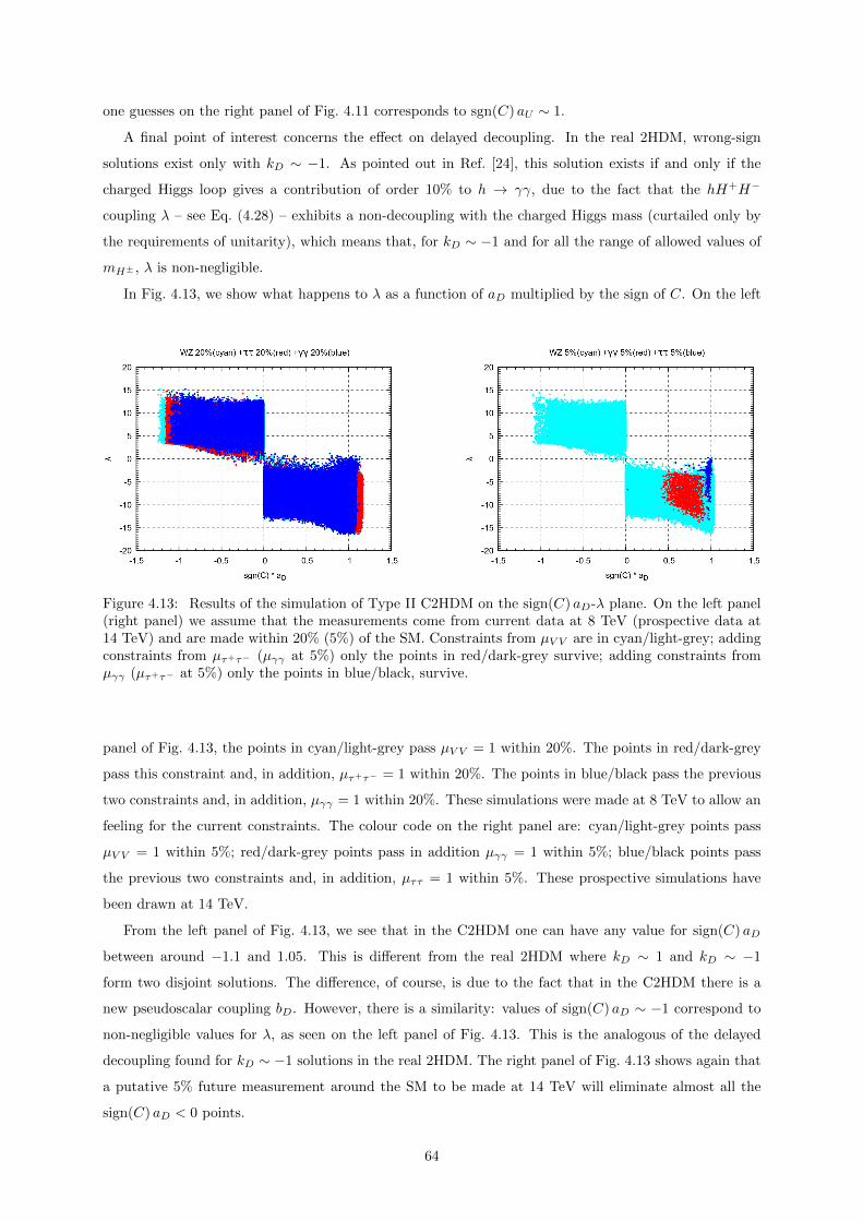
one guesses on the right panel of Fig. 4.11 corresponds to sgn(C) aU ∼ 1.
A final point of interest concerns the effect on delayed decoupling. In the real 2HDM, wrong-sign
solutions exist only with kD ∼ −1. As pointed out in Ref. [24], this solution exists if and only if the
charged Higgs loop gives a contribution of order 10% to h → γγ, due to the fact that the hH+H−
coupling λ – see Eq. (4.28) – exhibits a non-decoupling with the charged Higgs mass (curtailed only by
the requirements of unitarity), which means that, for kD ∼ −1 and for all the range of allowed values of
mH± , λ is non-negligible.
In Fig. 4.13, we show what happens to λ as a function of aD multiplied by the sign of C. On the left
Figure 4.13: Results of the simulation of Type II C2HDM on the sign(C) aD-λ plane. On the left panel(right panel) we assume that the measurements come from current data at 8 TeV (prospective data at14 TeV) and are made within 20% (5%) of the SM. Constraints from µV V are in cyan/light-grey; addingconstraints from µτ+τ− (µγγ at 5%) only the points in red/dark-grey survive; adding constraints fromµγγ (µτ+τ− at 5%) only the points in blue/black, survive.
panel of Fig. 4.13, the points in cyan/light-grey pass µV V = 1 within 20%. The points in red/dark-grey
pass this constraint and, in addition, µτ+τ− = 1 within 20%. The points in blue/black pass the previous
two constraints and, in addition, µγγ = 1 within 20%. These simulations were made at 8 TeV to allow an
feeling for the current constraints. The colour code on the right panel are: cyan/light-grey points pass
µV V = 1 within 5%; red/dark-grey points pass in addition µγγ = 1 within 5%; blue/black points pass
the previous two constraints and, in addition, µττ = 1 within 5%. These prospective simulations have
been drawn at 14 TeV.
From the left panel of Fig. 4.13, we see that in the C2HDM one can have any value for sign(C) aD
between around −1.1 and 1.05. This is different from the real 2HDM where kD ∼ 1 and kD ∼ −1
form two disjoint solutions. The difference, of course, is due to the fact that in the C2HDM there is a
new pseudoscalar coupling bD. However, there is a similarity: values of sign(C) aD ∼ −1 correspond to
non-negligible values for λ, as seen on the left panel of Fig. 4.13. This is the analogous of the delayed
decoupling found for kD ∼ −1 solutions in the real 2HDM. The right panel of Fig. 4.13 shows again that
a putative 5% future measurement around the SM to be made at 14 TeV will eliminate almost all the
sign(C) aD < 0 points.
64

4.4.6 Conclusions
The 125 GeV particle found at LHC could have a pseudoscalar component. We discuss in detail the
decay of a mixed scalar/pseudoscalar state into Zγ, which will be probed in the next LHC run. We
consider the constraints that current experiments impose on the four versions of the C2HDM and discuss
the prospects of future bounds, including h→ Zγ. This provides an update of Type I and Type II, and
the first discussion of current constraints on the Lepton Specific and Flipped C2HDM.
In the C2HDM, the parameter s2 measures the pseudoscalar content, with s2 = 0 (s2 = 1) correspond-
ing to a pure scalar (pseudoscalar). The fact that ATLAS has a rather large central value for µγγ places
strong limits on C2HDM, but it also disfavours the SM at 2-σ. But, even excluding this constraint, we
find that current experiments already disfavor a large pseudoscalar component |s2| > 0.85, at over 1-σ
level in all C2HDM versions.
As for future experimental reaches, we find that in all types of C2HDM a better measurement of
µbb(V h) ∼ 1 will exclude large values of the pseudoscalar component s2. Similarly, a measurement of
µZγ ∼ 1 will also exclude a very large s2 component. The Flipped C2HDM is special in that one can
have µτ+τ− ∼ 7 and, thus, the τ+τ− channel will be crucial in probing this model.
Finally, we have discussed the possibility that the scalar component of the Type II C2HDM h1qq
coupling (a) has a sign opposite to that in the SM. The fact that the C2HDM also has a pseudoscalar
component of the h1qq coupling (b) gives more room for differences than are possible within the Type II
real 2HDM. We found that the up quark coupling sgn(C) bU can have either sign, while sgn(C) aU must
be positive. If future experiments yield µV V , µγγ , and µτ+τ− within 5% of the SM, then sgn(C) bU can
still have either sign, but sgn(C) aU = 1 to very high precision, corresponding to the limit s1c2 = sβ . In
contrast, current experiments allow for either sign of both sgn(C) aD and sgn(C) bD, covering a rather
large region. However, if future experiments yield µV V , µγγ , and µτ+τ− within 5% of the SM, then
the region in the sgn(C) aD-sgn(C) bD plane reduces to a line, with most points concentrated around
sgn(C) aD ∼ 1. Still, there are a few points with sgn(C) aD ∼ −0.4, as long as sgn(C) bD ∼ −0.8 is
rather large.
4.5 Feynman rules for a general model with two Higgs doublets
This final section contains the relevant Feynman rules for the h→ Zγ decay, in the case where h has
both scalar and pseudoscalar components. These rules are written for a general model with two Higgs
doublets, where a, b, C and λ are real parameters. The specification of these parameters defines the
model. The C2HDM corresponds to the set of parameters given at the end of Section 4.1 (and one should
identify h with h1). The CP conserving 2HDM has b = 0 and a, C and λ given in Section 3.3. In the
special case of the SM, one simply has a = C = 1 and b = λ = 0.
We assume that the SM particles except the Higgs follow the usual Lagrangian, that there are H±
particles with the usual gauge-kinetic Lagrangian, and that the 125 GeV scalar/pseudoscalar Higgs h has
the following interactions with the fermions, the charged Higgs boson and the vectorial gauge bosons:
LY = −(√
2GF
) 12mf ψ (a+ ibγ5)ψ h, (4.27)
65
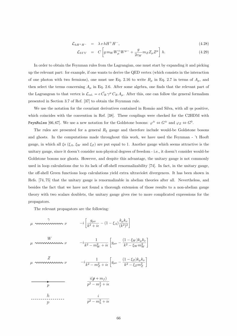
LhH+H− = λ v hH+H−, (4.28)
LhV V = C
[gmWW
+µ W
µ− +g
2cWmZZµZ
µ
]h. (4.29)
In order to obtain the Feynman rules from the Lagrangian, one must start by expanding it and picking
up the relevant part: for example, if one wants to derive the QED vertex (which consists in the interaction
of one photon with two fermions), one must use Eq. 2.16 to write Bµ in Eq. 2.7 in terms of Aµ, and
then select the terms concerning Aµ in Eq. 2.6. After some algebra, one finds that the relevant part of
the Lagrangean to that vertex is Lrel. = e CR γµ CRAµ. After this, one can follow the general formalism
presented in Section 3.7 of Ref. [37] to obtain the Feynman rule.
We use the notation for the covariant derivatives contained in Romao and Silva, with all ηs positive,
which coincides with the convention in Ref. [38]. These couplings were checked for the C2HDM with
FeynRules [66,67]. We use a new notation for the Goldstone bosons: ϕ± ⇔ G± and ϕZ ⇔ G0.
The rules are presented for a general Rξ gauge and therefore include would-be Goldstone bosons
and ghosts. In the computations made throughout this work, we have used the Feynman - ’t Hooft
gauge, in which all ξs (ξA, ξW and ξZ) are put equal to 1. Another gauge which seems attractive is the
unitary gauge, since it doesn’t consider non-physical degrees of freedom - i.e., it doesn’t consider would-be
Goldstone bosons nor ghosts. However, and despite this advantage, the unitary gauge is not commonly
used in loop calculations due to its lack of off-shell renormalizability [74]. In fact, in the unitary gauge,
the off-shell Green functions loop calculations yield extra ultraviolet divergences. It has been shown in
Refs. [74, 75] that the unitary gauge is renormalizable in abelian theories after all. Nevertheless, and
besides the fact that we have not found a thorough extension of those results to a non-abelian gauge
theory with two scalars doublets, the unitary gauge gives rise to more complicated expressions for the
propagators.
The relevant propagators are the following:
−i[
gµνk2 + iε
− (1− ξA)kµkν(k2)2
]µ ν
γ
−i 1
k2 −m2W + iε
[gµν −
(1− ξW )kµkνk2 − ξWm2
W
]µ ν
W
−i 1
k2 −m2Z + iε
[gµν −
(1− ξZ)kµkνk2 − ξZm2
Z
]µ ν
Z
i(/p+mf )
p2 −m2f + iεp
i
p2 −m2h + iε
h
p
66

i
p2 − ξZm2Z + iεp
ϕZ
i
p2 − ξWm2W + iεp
ϕ±
i
k2 − ξWm2W + iε
c±
k
The relevant vertices are the following:
−ie [gαβ(p− k)µ + gβµ(k − q)α + gµα(q − p)β ]
W−α
W+β
Aµ
p
k
q
−ig cos θW [gαβ(p− k)µ + gβµ(k − q)α + gµα(q − p)β ]
W−α
W+β
Zµ
p
k
q
−ieg cos θW [2gαβgµν − gαµgβν − gανgβµ]
W+α
Aµ
W−β
Zν
−i eQf γµ
ψf
ψf
Aµ−i g
cos θWγµ
(gfV −g
fAγ5
)ψf
ψf
Zµ
67
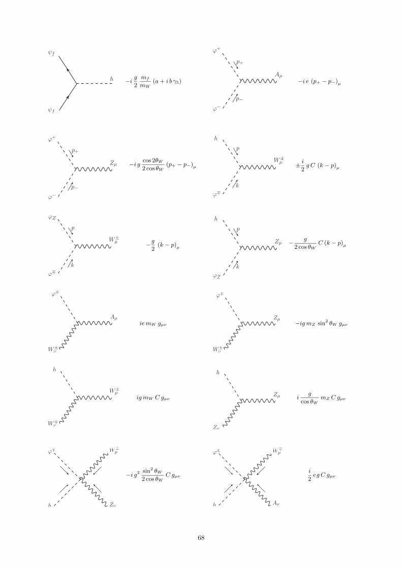
−i g2
mf
mW(a+ i b γ5)
ψf
ψf
h −i e (p+ − p−)µ
ϕ+
ϕ−
Aµ
p+
p−
−i g cos 2θW2 cos θW
(p+ − p−)µ
ϕ+
ϕ−
Zµ
p+
p−
± i2g C (k − p)µ
h
ϕ∓
W±µ
p
k
−g2
(k − p)µ
ϕZ
ϕ∓
W±µ
p
k
− g
2 cos θWC (k − p)µ
h
ϕZ
Zµ
p
k
iemW gµν
ϕ∓
W±ν
Aµ−ig mZ sin2 θW gµν
ϕ∓
W±ν
Zµ
ig mW C gµν
h
W∓ν
W±µ
ig
cos θWmZ C gµν
h
Zν
Zµ
−i g2 sin2 θW2 cos θW
C gµν
ϕ∓
h
W±µ
Zν
i
2eg C gµν
ϕ±
h
W∓µ
Aν
68
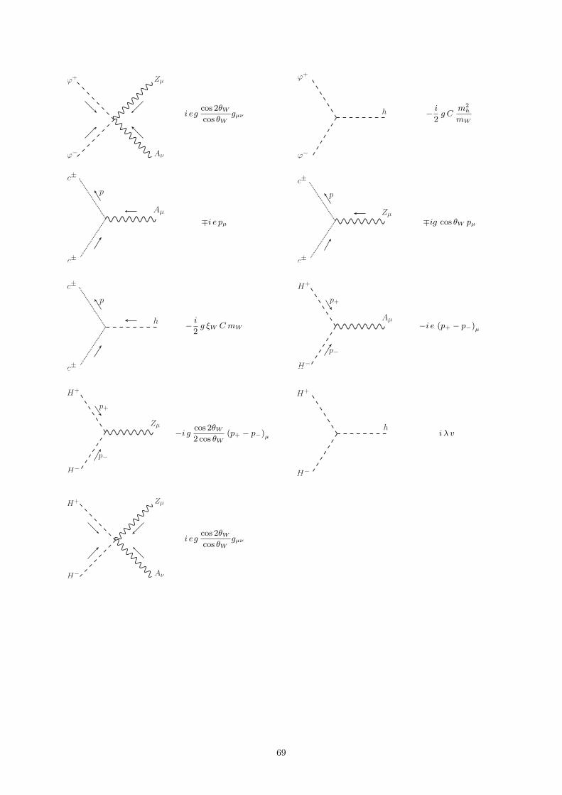
i egcos 2θWcos θW
gµν
ϕ+
ϕ−
Zµ
Aν
− i2g C
m2h
mW
ϕ+
ϕ−
h
∓i e pµ
c±
c±
Aµ
p
∓ig cos θW pµ
c±
c±
Zµ
p
− i2g ξW CmW
c±
c±
h
p
−i e (p+ − p−)µ
H+
H−
Aµ
p+
p−
−i g cos 2θW2 cos θW
(p+ − p−)µ
H+
H−
Zµ
p+
p−
i λ v
H+
H−
h
i egcos 2θWcos θW
gµν
H+
H−
Zµ
Aν
69
Appendix A
Further explanations in the 2HDM
A.1 Real and complex parameters; rephasing the fields
I would like to prove here why can we take λ5 in 3.3 to be real. Let us consider the first term in this
equation, m211Φ†1Φ1. If we redefine Φ1 in such a way that
Φ1 → eiθΦ1, (A.1)
this is, we rephase Φ1 (with θ being some arbitrary phase), then it is clear that the first term becomes
m211Φ†1Φ1 → m2
11Φ†1e−iθΦ1e
iθ = m211Φ†1Φ1, (A.2)
so that it is invariant under a rephasing of Φ1. This means that, in this first term, we have the freedom
to rephase Φ1 at our will, since it does not change the potential (Eq. 3.3). By the same token, the second
term is also invariant under rephasing of Φ2. In fact, if we rephase both Φ1 and Φ2 (each with its own
phase), all the first 6 terms in 3.3 stay invariant.
Before we look at the seventh term, we must remember that the potential V must be real. In Eq. 3.3,
each of the first 6 terms has a constant (which might, in principle, be real or complex) times a quantity
which has the form CC†, so that this quantity is necessarily real. It then follows, since V is real, that all
the constants of the first 6 terms must be real.
Let us now consider the seventh term. In this case, we no longer have the structure CC†: we now
have C + C†. In that case, though, its associated constant, λ5, can be complex - which means that it
has a modulus (say |λ5|) and a phase (say θ5). We then have λ5 = |λ5|eiθ5 . Here comes the trick: if we
rephase Φ1 and Φ2 in such a way that they absorb θ5, then λ5 becomes real. For example, if we state
that
Φ1 → eiθ54 Φ1, Φ2 → e−i
θ54 Φ2, (A.3)
then it follows that the seventh term becomes[ |λ5|eiθ52
(Φ†1Φ2
)2
+ h.c.
]→[ |λ5|eiθ5
2
(Φ†1e
−i θ54 Φ2e−i θ54
)2
+ h.c.
]=
[ |λ5|2
(Φ†1Φ2
)2
+ h.c.
]. (A.4)
so that λ5 lost its phase, this is, has become real. Please note that this trick is only possible because all
the terms in the potential are invariant under a rephasing.
70

We conclude that there exists a basis for the fields in which λ5 is real: this means that, although λ5 is
in general complex, its complex phase can be removed with a redefinition of the fields. Therefore, there
is no CP violation in the Higgs potential.
A.2 The condition for CP Violation in the C2HDM
I would like to prove here the reason why the condition arg(λ5) 6= 2 arg(m212) is necessary and sufficient
in order to have CP violation in the softly broken Z2 Higgs potential. Let us take Eq. 4.1: we are only
interested in the terms with complex parameters, which are
−m212
2
(Φ†1Φ2
)−(m2
12
)∗2
(Φ†2Φ1
)+λ5
2
(Φ†1Φ2
)2
+λ∗52
(Φ†2Φ1
)2
. (A.5)
Since m212 and λ5 are general complex numbers, we can write them as |m2
12|eiθ and |λ5|eiθ5 respectively,
where I have defined θ ≡ arg(m212) and θ5 ≡ arg(λ5). If we now rephase Φ1 and Φ2 according to1
Φ1 → Ψ1 = Φ1, Φ2 → Ψ2 = eiθΦ2, (A.6)
then Eq. A.5 becomes
− |m212|eiθ2
(Ψ†1Ψ2 e
iθ)− |m
212|e−iθ
2
(Ψ†2 e
−iθΨ1
)+|λ5|eiθ5
2
(Ψ†1Ψ2 e
iθ)2
+|λ5|e−iθ
2
(Ψ†2 e
−iθΨ1
)2
=− |m212|2
(Ψ†1Ψ2
)− |m
212|2
(Ψ†2Ψ1
)+|λ5|ei(θ5−2θ)
2
(Ψ†1Ψ2
)2
+|λ5|e−i(θ5−2θ)
2
(Ψ†2Ψ1
)2
,
(A.7)
so that, in this new basis, m212 is real since we have condensed all the phases in λ5, in which case it is
immediate to conclude that the relation
θ5 − 2θ 6= 0 ⇔ arg(λ5) 6= 2 arg(m2
12
)(A.8)
is a necessary and sufficient condition for CP violation: otherwise, there would exist a basis (in particular,
the Ψ1,Ψ2 one) in which there was no complex phase.
A.3 The Z2 symmetry; the different types of 2HDM
I would like to make a few remarks about the Z2 symmetry. I said previously that in order to avoid
FCNC at tree level in the 2HDM, one enforces the Z2 symmetry to the potential. But what does this
mean exactly? It means two things: first, each field Ψ of the Lagrangean L is transformed according to
one of the two options: either Ψ → Ψ or Ψ → −Ψ; second, only the terms which stay invariant under
that transformation are kept in L. Now, since there are two possible transformations for each field, one
must decide which one to pick.
In the scalar sector, it is generally used the transformation:(Φ1
Φ2
)→(−1 0
0 1
)(Φ1
Φ2
), (A.9)
1Remember that we can do such a rephasing since this leaves all the terms in the potential unchanged, as we have seenin Section A.1.
71
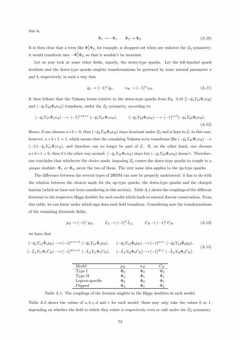
this is,
Φ1 → −Φ1 Φ2 → Φ2. (A.10)
It is then clear that a term like Φ†1Φ2, for example, is dropped out when one enforces the Z2 symmetry:
it would transform into −Φ†1Φ2, so that it wouldn’t be invariant.
Let us now look at some other fields, namely, the down-type quarks. Let the left-handed quark
doublets and the down-type quarks singlets transformations be governed by some natural parameter a
and b, respectively, in such a way that
qL → (−1)a qL, nR → (−1)b nR. (A.11)
It then follows that the Yukawa terms relative to the down-type quarks from Eq. 3.18 [(−qLYd1Φ1nR)
and (−qLYd2Φ2nR)] transform, under the Z2 symmetry, according to:
(−qLYd1Φ1nR) −→ (−1)a+b+1 (−qLYd1Φ1nR), (−qLYd2Φ2nR) −→ (−1)a+b(−qLYd2Φ2nR).
(A.12)
Hence, if one chooses a+b = 0, then (−qLYd2Φ2nR) stays invariant under Z2 and is kept in L; in this case,
however, a+ b+ 1 = 1, which means that the remaining Yukawa term transforms like (−qLYd1Φ1nR) −→(−1)(−qLYd1Φ1nR), and therefore can no longer be part of L. If, on the other hand, one chooses
a+b+1 = 0, then it’s the other way around: (−qLYd1Φ1nR) stays but (−qLYd2Φ2nR) doesn’t. Therefore,
one concludes that whichever the choice made, imposing Z2 causes the down-type quarks to couple to a
unique doublet: Φ1 or Φ2, never the two of them. The very same idea applies to the up-type quarks.
The difference between the several types of 2HDM can now be properly understood: it has to do with
the relation between the choices made for the up-type quarks, the down-type quarks and the charged
leptons (which we have not been considering in this section). Table A.1 shows the couplings of the different
fermions to the respective Higgs doublet for each model which leads to natural flavour conservation. From
this table, we can know under which sign does each field transform. Considering now the transformations
of the remaining fermionic fields,
pR → (−1)c pR, LL → (−1)d LL, CR → (−1)e CR. (A.13)
we have that
(−qLYu1Φ1pR) −→ (−1)a+c+1 (−qLYu1Φ1pR), (−qLYu2Φ2pR)−→ (−1)a+c (−qLYu2Φ2pR),
(−LLYl1Φ1CR) −→ (−1)d+e+1 (−LLYl1Φ1CR), (−LLYl2Φ2CR)−→ (−1)d+e (−LLYl2Φ2CR).(A.14)
Model pR nR CRType I Φ2 Φ2 Φ2
Type II Φ2 Φ1 Φ1
Lepton-specific Φ2 Φ2 Φ1
Flipped Φ2 Φ1 Φ2
Table A.1: The couplings of the fermion singlets to the Higgs doublets in each model.
Table A.2 shows the values of a, b, c, d and e for each model; these may only take the values 0 or 1,
depending on whether the field to which they relate is respectively even or odd under the Z2 symmetry.
72
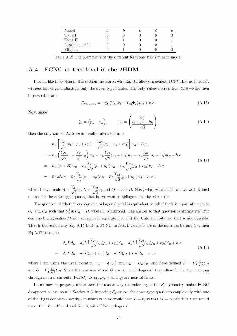
Model a b c d eType I 0 0 0 0 0Type II 0 1 0 0 1Lepton-specific 0 0 0 0 1Flipped 0 1 0 0 0
Table A.2: The coefficients of the different fermionic fields in each model.
A.4 FCNC at tree level in the 2HDM
I would like to explain in this section the reason why Eq. 3.1 allows in general FCNC. Let us consider,
without loss of generalization, only the down-type quarks. The only Yukawa terms from 3.18 we are then
interested in are
LYukawan = −qL (Yd1Φ1 + Yd2Φ2)nR + h.c.. (A.15)
Now, since
qL =(pL nL
), Φi =
φ+i
vi + ρi + iηi√2
, (A.16)
then the only part of A.15 we are really interested in is
− nL[Yd1√
2(v1 + ρ1 + iη1) +
Yd2√2
(v2 + ρ2 + iη2)
]nR + h.c.
=− nL(Yd1√
2v1 +
Yd2√2v2
)nR − nL
Yd1√2
(ρ1 + iη1)nR − nLYd2√
2(ρ2 + iη2)nR + h.c.
=− nL (A+B)nR − nLYd1√
2(ρ1 + iη1)nR − nL
Yd2√2
(ρ2 + iη2)nR + h.c.
=− nLMnR − nLYd1√
2(ρ1 + iη1)nR − nL
Yd2√2
(ρ2 + iη2)nR + h.c.,
(A.17)
where I have made A =Yd1√
2v1, B =
Yd2√2v2 and M = A+B. Now, what we want is to have well defined
masses for the down-type quarks, that is, we want to bidiagonalize the M matrix.
The question of whether one can one bidiagonalize M is equivalent to ask if there is a pair of matrices
UL and UR such that U†LMUR = D, where D is diagonal. The answer to that question is affirmative. But
can one bidiagonalize M and diagonalize separately A and B? Unfortunately no: that is not possible.
That is the reason why Eq. A.15 leads to FCNC: in fact, if we make use of the matrices UL and UR, then
Eq.A.17 becomes:
− dLDdR − dLU†LYd1√
2UR(ρ1 + iη1)dR − dLU†L
Yd2√2UR(ρ2 + iη2)dR + h.c.
=− dLDdR − dLF (ρ1 + iη1)dR − dLG(ρ2 + iη2)dR + h.c.,
(A.18)
where I am using the usual notation nL = dLU†L and nR = URdR, and have defined F = U†L
Yd1√2UR
and G = U†LYd2√
2UR. Since the matrices F and G are not both diagonal, they allow for flavour changing
through neutral currents (FCNC), as ρ1, ρ2, η1 and η2 are neutral fields.
It can now be properly understood the reason why the enforcing of the Z2 symmetry makes FCNC
disappear: as can seen in Section A.3, imposing Z2 causes the down-type quarks to couple only with one
of the Higgs doublets - say Φ2 - in which case we would have B = 0, so that M = A, which in turn would
mean that F = M = A and G = 0, with F being diagonal.
73

A.5 Equivalence between the definitions of CP Violation
In Chapter 4, I have given two definitions of CP Violation, namely, that it corresponds, on the one
hand, to have an irremovable2 complex phase, and, on the other, to have a certain field with scalar and
pseudoscalar components. I use this section to prove their equivalence.
Let us suppose a real spin-0 field, ϕ. We might use the Yukawa sector of the theory to determine
whether ϕ is scalar or pseudoscalar: all we have to do is study the interaction term between ϕ and a
fermionic field ψ. What is the form of such an interaction term? Lorentz invariance requires it to be like
ψ Γj ψ, with j = S, V, T,A, P, (A.19)
where
ΓS = 1, ΓVµ = γµ, ΓTµν = σµν =i
2[γµ, γν ] , ΓAµ = γ5γµ, ΓP = γ5, (A.20)
where 1 represents the 4×4 identity matrix and S, V, T,A, P stand for scalar, vector, tensor, axial vector
(or pseudovector) and pseudoscalar, respectively. Our interaction might in fact be a combination of these
structures. Actually, the structures ΓVµ , ΓTµν and ΓAµ are excluded, since they would not have any Lorentz
index with which they could contract (so that they would not in fact be Lorentz invariant). Our most
general interaction term between ϕ and ψ is thus:
α ψϕψ + β ψϕγ5ψ + h.c., (A.21)
where α and α are arbitrary complex constants. We then have:
α ψϕψ + β ψϕγ5ψ + h.c. = α ψϕψ + β ψϕγ5ψ +(α ψϕψ + β ψϕγ5ψ
)†=
= α ψϕψ + β ψϕγ5ψ + α∗ ψϕψ − β∗ ψϕγ5ψ = (α+ α∗) ψϕψ + (β − β∗) ψϕγ5ψ =
= ψ (a+ ibγ5)ϕψ,
(A.22)
where I have used the facts that ϕ is real and γ5 anticommutes with γ0, and where I have defined
a := (α+ α∗) = Re (α+ α∗) and b := β−β∗i = Im (β − β∗), so that a, b ∈ R.
One should now ask what is the action of the operator CP on this term. One has3:
CP[ψ (a+ ibγ5)ϕψ
]= ψ (a− ibγ5)ϕψ, (A.23)
where we have used the distributive property of the operator CP . Using this last property, and given
that CP[ψψ]
= λψψ ψψ = ψψ (where λ represents the CP eigenvalue), we conclude that, if we want the
Lagrangean to be CP conserving (so that so that it has CP eigenvalue equal to 1 and every field has a
well-defined CP eigenvalue), we then have two options for the CP eigenvalue of ϕ: either ϕ couples to
the a term and not to the b term, in which case our requisite λL = 1 implies
λψ ϕψ = 1 ⇔ λψ ψ λϕ = 1 ⇔ λϕ = 1, (A.24)
so that ϕ is a scalar, or else ϕ couples to the b term and not to the a term, in which case our requisite
λL = 1 implies
λψ ϕ γ5 ψ = 1 ⇔ λψ ψ λγ5 λϕ = 1 ⇔ λϕ = −1, (A.25)
2Irremovable in the sense that there is no basis in which the phase disappears.3See, for example, Eqs. 3.74 and 3.75 from Ref. [72].
74

so that ϕ is a pseudoscalar. We thus see that ϕ cannot couple to both a and b terms, since that would
require it to have both λϕ = ±1 (which is not possible because, as we have seen, in a CP conserving
Lagrangean every field must have a well-defined [i.e. unique] CP eigenvalue).
The scenario changes when we do not impose CP conservation of the Lagrangean. In this case, we
no longer have the restriction λL = 1, so that ϕ can now couple to both a and b terms. This means
that ϕ has a component which it could have if there was CP conservation and if ϕ was scalar (namely,
that which makes it couple to the a term), and ϕ also has a component which it could have if there was
CP conservation and if ϕ was pseudoscalar (namely, that which makes it couple to the b term). I am
using this complicated language (instead of simply saying that, in the CP violating case, ϕ has both a
scalar and a pseudoscalar component) because, when there is CP violation, the expressions “scalar” and
“pseudoscalar” make no sense [41]; therefore, the most we can say is by analogy to the CP conserving
case, where those expressions make sense. One should thus replace our second definition of CP violation
“when a certain field has scalar and pseudoscalar components” by “when a certain field behaves both like
a scalar and a pseudoscalar field in a CP conserving situation”.
It should be now clear why the two CP violation definitions are equivalent. When there is CP
violation, ϕ couples in general to both a and b terms (second definition); but as it is patent in the last
line of Eq. A.22, there is a complex phase between the two (first definition).
75

Appendix B
Useful formulae concerning Higgs
production and decays
In this appendix, we present several formulae which allowed us to perform the numerical calculi
throughout this work. They apply to the C2HDM (which is the most general model studied), so that
they follow the notation of Section 4.1. The expressions relative to the h → Zγ decay, having been the
focus of this thesis, were presented in the main text; I dedicate this appendix to the remaining expressions,
which include both the production and the decays.
B.1 Higgs production expressions
The production cross section due to gluon-gluon fusion and associated production with heavy quarks
is given by
σ(gg → h) =GFα
2s
512√
2π
(|Xgg
F |2 + |Y ggF |2), (B.1)
where αs is the QCD coupling constant, and
XggF = −
∑q
2aq τq [1 + (1− τq)f(τq)] ,
Y ggF = −∑q
2bq τqf(τq), (B.2)
where the function f is defined in Eq. 2.58 and the sums run only over quarks q. In this work, we define
τ as
τ = 4m2/m2h, (B.3)
where m is the mass of the relevant particle (and mh = 125 GeV). This is the notation of [38]. In [14,27,79]
the notation is τ(theirs) = τ−1. The functions of Eq. B.2 are dominated by the triangle with top quark
in the loop, and, depending on tanβ, also by the triangle with bottom quark in the loop. Thus, we can
useσ(gg → h)
σSM(gg → h)=|atA1/2(τt) + abA1/2(τb)|2 + |btAA1/2(τt) + bbA
A1/2(τb)|2
|A1/2(τt) +A1/2(τb)|2, (B.4)
76

where
A1/2(τq) = = 2τq [1 + (1− τq)f(τq)] ,
AA1/2(τq) = 2τqf(τq) . (B.5)
For the vector boson fusion (VBF) and V h productions, we find
σVBF
σSMVBF
=σVh
σSMVh
= C2, (B.6)
while, for the bb production,σ(bb→ h)
σSM(bb→ h)= a2 + b2. (B.7)
We point out that the expressions shown here hold for any model with the effective Lagrangians of
Eqs. (4.27)-(4.29). Also, there is no interference between the scalar a couplings and the pseudoscalar b
couplings in Eqs. (B.8) or (B.7).
B.2 Higgs decays expressions
The decays into fermions are given by
Γ(h→ ff) = NcGF m
2f
4√
2πmh
[a2β3
f + b2βf], (B.8)
where Nc = 3 (Nc = 1) for quarks (leptons) and βf =√
1− 4m2f/m
2h =
√1− τ . The decays into two
vector bosons are given by
Γ(h→ V (∗)V (∗)) = C2 ΓSM(h→ V (∗)V (∗)), (B.9)
and the partial decay widths in the SM-Higgs case in the two-, three- and four-body approximations,
ΓSM(h→ V (∗)V (∗)), can be found in Section I.2.2 of Ref. [27]. The decay into two gluons obeys to
Γ(h→ gg) =GFα
2Sm
3h
64√
2π3
(|Xgg
F |2 + |Y ggF |2), (B.10)
where XggF and Y ggF are the same of Eq. B.2. We now dedicate some space to the h → γγ decay at
one-loop, since its expressions are lengthier due to its loop mediated character.
B.2.1 The h→ γγ case
The h→ γγ decay, just like the h→ Zγ, does not happen at tree level. The 1PI diagrams at one-loop
are the same of those depicted in Figs. 2.2 and 3.1, except that the Z boson is replaced with a second
photon. We thus divide our analysis into three parts: the fermion mediated loop diagrams, the vectorial
boson mediated loop diagrams and the charged Higgs mediated loop diagrams.
Fermions
The one-loop amplitude reads
MγγF ≡ (q1 · q2 ε1 · ε2 − q1 · ε2 q2 · ε1) cγγF + εµναβ q
µ1 qν2 εα1 εβ2 dγγF , (B.11)
77
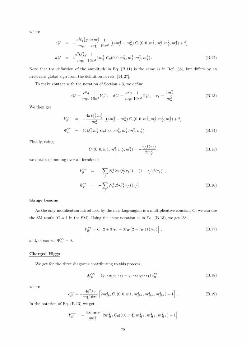
where
cγγF = −e2Q2
fg
mW
4am2f
m2h
1
16π2
[(4m2
f −m2h
)C0(0, 0,m2
h,m2f ,m
2f ,m
2f ) + 2
],
dγγF = 4e2Q2
fg
mW
1
16π2bm2
f C0(0, 0,m2h,m
2f ,m
2f ,m
2f ) . (B.12)
Note that the definition of the amplitude in Eq. (B.11) is the same as in Ref. [38], but differs by an
irrelevant global sign from the definition in refs. [14,27].
To make contact with the notation of Section 4.3, we define
cγγF ≡e2g
mW
1
16π2Y γγF , dγγF ≡
e2g
mW
1
16π2ΨγγF , τf ≡
4m2f
m2h
. (B.13)
We then get
Y γγF = −4aQ2
f m2f
m2h
[(4m2
f −m2h
)C0(0, 0,m2
h,m2f ,m
2f ,m
2f ) + 2
]ΨγγF = 4bQ2
f m2f C0(0, 0,m2
h,m2f ,m
2f ,m
2f ). (B.14)
Finally, using
C0(0, 0,m2h,m
2f ,m
2f ,m
2f ) = −τff(τf )
2m2f
, (B.15)
we obtain (summing over all fermions)
Y γγF = −∑f
Nfc 2aQ2
f τf [1 + (1− τf )f(τf )] ,
ΨγγF = −
∑f
Nfc 2bQ2
f τff(τf ) . (B.16)
Gauge bosons
As the only modification introduced by the new Lagrangian is a multiplicative constant C, we can use
the SM result (C = 1 in the SM). Using the same notation as in Eq. (B.13), we get [38],
Y γγW = C[2 + 3τW + 3τW (2− τW )f(τW )
], (B.17)
and, of course, ΨγγW = 0.
Charged Higgs
We get for the three diagrams contributing to this process,
MγγH = (q1 · q2 ε1 · ε2 − q1 · ε2 q2 · ε1) cγγH , (B.18)
where
cγγH = − 4e2λv
m2h16π2
[2m2
H±C0(0, 0,m2h,m
2H± ,m
2H± ,m
2H±) + 1
]. (B.19)
In the notation of Eq. (B.13) we get
Y γγH =− 4λmW v
gm2h
[2m2
H±C0(0, 0,m2h,m
2H± ,m
2H± ,m
2H±) + 1
]78

=− λv2
2m2H±
τ±[1− τ±f(τ±)
]. (B.20)
Note that this is in agreement with Eq. (2.17) of Ref. [38], despite the apparent sign difference, because
our definition of the coupling, in Eq. (4.28), also differs in sign from their Eq. (2.15). So we are in
complete agreement with Ref. [38]. With respect to Ref. [14], if we compare with their eqs. (A.8) and
(A.4), again we differ by a global sign and we are, therefore, in agreement. The same holds for Ref. [27].
Total Width
The total width, as in the case h→ Zγ, is given by
Γ =1
8π
|~q1|m2h
|M |2 . (B.21)
In this case, however, |~q1| = mh/2, and
|M |2 =
(eg
16π2mW
)2 [|Y γγF + Y γγW + Y γγH |2 (q1 · q1gµν − q1µq2ν) (q1 · q1gµ′ν′ − q1µ′q2ν′)
(−gµµ′)(−gνν′)
+|ΨγγF |2 εµναβqµ1 qν2 εµ′ν′α′β′qµ
′
1 qν′
2 (−gαα′)(−gββ′)]
=
(eg
16π2mW
)2m4h
2
(|Y γγF + Y γγW + Y γγH |2 + |Ψγγ
F |2). (B.22)
Putting everything together, and including the factor 1/2 for identical particles, we get the final result
Γ(h→ γγ) =GFα
2m3h
128√
2π3
∑f
(|Y γγF + Y γγW + Y γγH |2 + |Ψγγ
F |2). (B.23)
B.3 Relation between the Passarino-Veltman functions and other
loop functions
When we compute the one-loop diagrams, as we did, using FeynCalc [35], the result is naturally
presented in terms of the well-known Passarino-Veltman integrals [36]. These are in general complicated
functions of the external momenta and masses and usually only possible to be expressed in terms of
very complicated functions. Normally, it is better to evaluate them numerically and for that there is the
package LoopTools [76]. However for special situations, like zero external momenta or equal masses in
the loops, these loop integrals have simpler forms and can be expressed in terms of simple functions. This
is the case for the loops studied here and we present in this appendix the relations of these Passarino-
-Veltman integrals with other representations found in the literature.
B.3.1 The integrals for h→ γγ
In this decay, all results can be expressed in terms of the Passarino-Veltman integral C0(0, 0,m2h,m
2,m2,
m2), where m is the mass of the particle running in the loop. We have already given in Eq. (B.15) the
79

relation with the function f(τ) defined in the Higgs Hunter’s Guide [38],
C0(0, 0,m2h,m
2,m2,m2) = −τf(τ)
2m2, τ =
4m2
m2h
, (B.24)
where f(τ) is defined in Eq. 2.58.
B.3.2 The integrals for h→ Zγ
To compare our results in terms of the Passarino-Veltman functions with those of Ref. [38], we notice
that
C0(m2Z , 0,m
2h,m
2,m2,m2) = − 1
m2I2(τ, λ) , (B.25)
∆B0 = −m2h −m2
Z
m2Z
− (m2h −m2
Z)2
2m2m2Z
I1(τ, λ) + 2m2h −m2
Z
m2Z
I2(τ, λ) , (B.26)
where I1 and I2 are defined in Eqs. 2.56 and 2.57. We have checked these equations numerically with the
help of the package LoopTools [76].
Using these relations, one can check that our Eqs. 2.50, 2.51, 2.52 and 3.40 agree with Eqs. (C.12),
(C.13) and (C.14) of Ref. [38] up to an overall sign. We notice that our coupling to the charged Higgs
translate into their notation
λv → −RhH± . (B.27)
There is no equivalent result to our Eq. (4.23) in Ref. [38], but we are in agreement with Ref. [27] up to
global signs. However, we warn the reader that the definitions of I1, I2 and g(τ) in Eqs. (2.55) and (2.56)
of Ref. [27] are not consistent.
80

Appendix C
Computational programs
I would like to give a brief description of the computational programs used throughout this work,
explaining what they were useful for. I present the different programs in a logical order. I shall not
be able to explain in all the detail everything I wanted to, since that would require too much space.
However, my supervisor Jorge C. Romao provides a list of very helpful “howtos”, which can be found at
http://porthos.ist.utl.pt/mediawiki/index.php/HowTo.
QGRAF
The first program one should take into account when studying a certain process in Quantum Field
Theory is QGRAF [32]. In fact, when the process is loop mediated, there are typically dozens of diagrams,
thus being difficult to identify them all. QGRAF solves this problem by automatically discriminating all
the diagrams involved.
The program generates Feynman diagrams through symbolic expressions for any process, although
it does not present the diagrams graphically. Using these symbolic expressions, one can then draw the
Feynman diagrams using for example the program JaxoDraw.
QGRAF might be downloaded at http://cfif.ist.utl.pt/~paulo/qgraf.html and run on Windows
(instructions on how to do it might be found at http://porthos.ist.utl.pt/CTQFT/files/QGRAF_
wininstr_en.pdf). Several examples and useful models have been developed by my supervisor Jorge C.
Romao and are available at http://porthos.ist.utl.pt/CTQFT/node7.html.
JaxoDraw
JaxoDraw [77] is a Java program for drawing Feynman diagrams. It might be downloaded at http:
//jaxodraw.sourceforge.net/download/exe.html.
Feynrules
Feynrules [66, 67] is a Mathematica [78] package that allows the calculation of Feynman rules in
momentum space. It might be downloaded at https://feynrules.irmp.ucl.ac.be/. My supervisor
Jorge C. Romao has developed one Feynrules file for the C2HDM, which we have used to check our
81

couplings and write down the Feynman rules of the theory. Feynrules also is very useful after one has
drawn the diagrams and wants to write down the amplitudes, which one can do using Feyncalc.
Feyncalc
Feyncalc [35] is a Mathematica [78] package for algebraic calculations in elementary particle physics.
It might be downloaded at http://feyncalc.org/. It is extremely useful in loop integrals. After knowing
the different Feynman diagrams contributing to a given process, one can use Feyncalc to compute the
amplitude associated with the each one. Particularly useful were the functions Oneloop and PaVeReduce:
when one wants to compute a 1-loop integral, Feyncalc default function is Oneloop, which rewrites the
integral in terms of the Passarino-Veltman [36] functions. Then, one can use the function PaVeReduce to
obtain the result in terms of the Passarino-Veltman scalar functions A0, B0, C0, etc. It should be stressed,
however, that this procedure is not numerical: all one does is to rewrite some complicated integrals in
terms of some scalar functions. If one wants a numerical result, then one should use LoopTools.
Fortran and LoopTools
LoopTools [76] is a Fortran package for the numerical evaluation of one-loop integrals. It can be
downloaded at http://www.feynarts.de/looptools/. All the implementation of the model, the Higgs
decay functions, the theoretical constraints, etc, which allowed us to generate points for the scatterplots
throughout this thesis have been built on a Fortran code. We used the results of Feyncalc - which gave
us the amplitudes written in terms of the Passarino-Veltman scalar functions - and inserted them into
our code, which yielded numerical values due to LoopTools. Fortran thus generates a text file, which
can be used as input for another program - as Gnuplot - in order to create graphics and scatterplots.
Gnuplot
Gnuplot is a command-line program very useful to generate plots of data. It can be downloaded
at http://www.gnuplot.info/. Particularly useful to use with Gnuplot is Awk (http://www.gnu.org/
software/gawk/manual/gawk.html), which allows the user to select particular records in the text files
and filtering results.
82
Bibliography
[1] D. Fontes, J. C. Romao and J. P. Silva, Phys. Rev. D 90 (2014) 015021 [arXiv:1406.6080 [hep-ph]].
[2] D. Fontes, J. C. Romao and J. P. Silva, arXiv:1408.2534 [hep-ph].
[3] G. Aad et al. [ATLAS Collaboration], Phys. Lett. B 716 (2012) 1 [arXiv:1207.7214 [hep-ex]].
[4] S. Chatrchyan et al. [CMS Collaboration], Phys. Lett. B 716 (2012) 30 [arXiv:1207.7235 [hep-ex]].
[5] T. Aaltonen et al. [CDF and D0 Collaborations], Phys. Rev. Lett. 109 (2012) 071804
[arXiv:1207.6436 [hep-ex]].
[6] T. Aaltonen et al. [CDF and D0 Collaborations], Phys. Rev. D 88 (2013) 5, 052014 [arXiv:1303.6346
[hep-ex]].
[7] [ATLAS Collaboration], ATLAS-CONF-2013-034.
The ATLAS collaboration, ATLAS-CONF-2013-072.
The ATLAS collaboration, ATLAS-CONF-2013-012.
ATLAS Collaboration, https://twiki.cern.ch/twiki/bin/view/AtlasPublic/HiggsPublicResults.
[8] M. E. Chasco [CMS Collaboration], arXiv:1310.1002 [hep-ex].
CMS-PAS-HIG-13-005.
V. Khachatryan et al. [ CMS Collaboration], arXiv:1407.0558 [hep-ex].
CMS Collaboration, https://twiki.cern.ch/twiki/bin/view/CMSPublic/PhysicsResultsHIG.
[9] S. Chatrchyan et al. [CMS Collaboration], Phys. Rev. D 89 (2014) 012003 [arXiv:1310.3687 [hep-
ex]].
[10] B. Tuchming [CDF and D0 Collaborations], arXiv:1405.5058 [hep-ex].
[11] ATLAS collaboration. Talk given by Marumi Kado at ICHEP2014, July 2014, Valencia, Spain.
[12] CMS collaboration. Talk given by A. David at ICHEP2014, July 2014, Valencia, Spain.
[13] P. M. Ferreira, R. Santos, M. Sher and J. P. Silva, Phys. Rev. D 85 (2012) 077703 [arXiv:1112.3277
[hep-ph]].
[14] A. Barroso, P. M. Ferreira, R. Santos and J. P. Silva, Phys. Rev. D 86 (2012) 015022
[arXiv:1205.4247 [hep-ph]].
83
[15] A. Alves, E. R. Barreto and A. G. Dias, arXiv:1312.5333 [hep-ph].
[16] G. Aad et al. [ATLAS Collaboration], Phys. Lett. B 732 (2014) 8 [arXiv:1402.3051 [hep-ex]].
[17] S. Chatrchyan et al. [CMS Collaboration], Phys. Lett. B 726 (2013) 587 [arXiv:1307.5515 [hep-ex]].
[18] T. D. Lee, Phys. Rev. D 8 (1973) 1226.
[19] G. Aad et al. [ATLAS Collaboration], Phys. Lett. B 726 (2013) 88 [arXiv:1307.1427 [hep-ex]].
[20] S. Chatrchyan et al. [CMS Collaboration], Phys. Rev. D 89 (2014) 092007 [arXiv:1312.5353 [hep-
ex]].
[21] D. Carmi, A. Falkowski, E. Kuflik and T. Volansky, JHEP 1207 (2012) 136 [arXiv:1202.3144 [hep-
ph]].
[22] C. -W. Chiang and K. Yagyu, JHEP 1307 (2013) 160 [arXiv:1303.0168 [hep-ph]].
[23] A. Barroso, P. M. Ferreira, R. Santos, M. Sher and J. P. Silva, arXiv:1304.5225 [hep-ph], talk
given by R. Santos at Toyama International Workshop on Higgs as a Probe of New Physics (13-16,
February, 2013).
[24] P. M. Ferreira, J. F. Gunion, H. E. Haber and R. Santos, Phys. Rev. D 89 (2014) 115003
[arXiv:1403.4736 [hep-ph]].
[25] J. C. Romao and J. P. Silva, Int. J. Mod. Phys. A 27 (2012) 1230025 [arXiv:1209.6213 [hep-ph]].
[26] J. P. Silva, hep-ph/0410351.
[27] A. Djouadi, Phys. Rept. 457 (2008) 1 [hep-ph/0503172].
[28] M. Spira, hep-ph/9510347.
[29] R. V. Harlander, S. Liebler and H. Mantler, Computer Physics Communications 184 (2013) 1605
[arXiv:1212.3249 [hep-ph]].
[30] https://twiki.cern.ch/twiki/bin/view/LHCPhysics/CrossSectionsFigures .
[31] K. G. Chetyrkin, Phys. Lett. B 404 (1997) 161 [hep-ph/9703278].
[32] P. Nogueira, J. Comput. Phys. 105 (1993) 279.
[33] J. C. Romao, Introducao a Teoria do Campo, http://porthos.ist.utl.pt/ftp/textos/itc.pdf
[34] W. Greiner, J. Reinhart, Quantum Electrodynamics, Third Edition (Springer-Verlag, Ger-
many, 2003)
[35] R. Mertig, M. Bohm and A. Denner, Feyn Calc - Computer-algebraic calculation of Feynman am-
plitudes, Comput. Phys. Commun. 64 (1991) 345. See http://www.feyncalc.org.
[36] G. Passarino and M. J. G. Veltman, Nucl. Phys. B 160 (1979) 151.
84

[37] J. C. Romao, Advanced Quantum Field Theory, http://porthos.ist.utl.pt/ftp/textos/tca.
[38] J. Gunion, H. Haber, G. Kane, S. Dawson, The Higgs Hunter’s Guide (Addison-Wesley Publishing
Company, USA, 1990)
[39] S. Sakakibara, Phys. Rev. D 24 (1981) 1149.
[40] S. L. Glashow and S. Weinberg, Phys. Rev. D 15 (1977) 1958; E. A. Paschos, Phys. Rev. D 15
(1977) 1966.
[41] T. D. Lee and G. C. Wick, Phys. Rev. 148 (1966) 1385.
[42] L. Lavoura and J. P. Silva, Phys. Rev. D 50 (1994) 4619 [hep-ph/9404276].
[43] F. J. Botella and J. P. Silva, Phys. Rev. D 51 (1995) 3870 [hep-ph/9411288].
[44] G. C. Branco, P. M. Ferreira, L. Lavoura, M. N. Rebelo, M. Sher and J. P. Silva, Phys. Rept. 516
(2012) 1 [arXiv:1106.0034 [hep-ph]].
[45] I. P. Ivanov, Phys. Rev. D 77 (2008) 015017 [arXiv:0710.3490 [hep-ph]].
[46] A. Barroso, P. M. Ferreira, I. P. Ivanov and R. Santos, JHEP 1306 (2013) 045 [arXiv:1303.5098
[hep-ph]].
[47] N. G. Deshpande and E. Ma, Phys. Rev. D 18 (1978) 2574.
[48] J. F. Gunion and H. E. Haber, Phys. Rev. D 67 (2003) 075019 [hep-ph/0207010].
[49] S. Kanemura, T. Kubota and E. Takasugi, Phys. Lett. B 313 (1993) 155 [hep-ph/9303263].
[50] A. G. Akeroyd, A. Arhrib and E. -M. Naimi, Phys. Lett. B 490 (2000) 119 [hep-ph/0006035].
[51] I. F. Ginzburg and I. P. Ivanov, hep-ph/0312374.
[52] B. W. Lee, C. Quigg and H. B. Thacker, Phys. Rev. Lett. 38 (1977) 883.
[53] B. W. Lee, C. Quigg and H. B. Thacker, Phys. Rev. D 16 (1977) 1519.
[54] I. F. Ginzburg and M. Krawczyk, Phys. Rev. D 72 (2005) 115013 [hep-ph/0408011].
[55] A. Arhrib, M. Capdequi Peyranere, W. Hollik and S. Penaranda, Phys. Lett. B 579 (2004) 361
[hep-ph/0307391].
[56] M. E. Peskin and T. Takeuchi, Phys. Rev. Lett. 65 (1990) 964.
[57] M. E. Peskin and T. Takeuchi, Phys. Rev. D 46 (1992) 381.
[58] M. Baak, M. Goebel, J. Haller, A. Hoecker, D. Ludwig, K. Moenig, M. Schott and J. Stelzer, Eur.
Phys. J. C 72 (2012) 2003 [arXiv:1107.0975 [hep-ph]].
85

[59] M. Baak, M. Goebel, J. Haller, A. Hoecker, D. Kennedy, R. Kogler, K. Moenig and M. Schott et
al., Eur. Phys. J. C 72 (2012) 2205 [arXiv:1209.2716 [hep-ph]].
[60] A. Arhrib, E. Christova, H. Eberl and E. Ginina, JHEP 1104 (2011) 089 [arXiv:1011.6560 [hep-ph]].
[61] H. E. Haber and H. E. Logan, Phys. Rev. D 62 (2000) 015011 [hep-ph/9909335].
[62] T. Hermann, M. Misiak and M. Steinhauser, JHEP 1211 (2012) 036 [arXiv:1208.2788 [hep-ph]].
[63] F. Mahmoudi, talk given at Prospects For Charged Higgs Discovery At Colliders (CHARGED 2012),
8-11 October, Uppsala, Sweden.
[64] G. Aad et al. [ATLAS Collaboration], Search for charged Higgs bosons decaying via H+ → τν in
top quark pair events using pp collision data at√s = 7 TeV with the ATLAS detector, JHEP 1206
(2012) 039 [arXiv:1204.2760 [hep-ex]].
[65] S. Chatrchyan et al. [CMS Collaboration], Search for a light charged Higgs boson in top quark decays
in pp collisions at√s = 7 TeV, JHEP 1207 (2012) 143 [arXiv:1205.5736 [hep-ex]].
[66] N. D. Christensen and C. Duhr, Comput. Phys. Commun. 180 (2009) 1614 [arXiv:0806.4194 [hep-
ph]].
[67] A. Alloul, N. D. Christensen, C. Degrande, C. Duhr and B. Fuks, Comput. Phys. Commun. 185
(2014) 2250 [arXiv:1310.1921 [hep-ph]].
[68] N. Craig, J. Galloway and S. Thomas, arXiv:1305.2424 [hep-ph].
[69] G. Bhattacharyya, D. Das, P. B. Pal and M. N. Rebelo, JHEP 1310, 081 (2013) [arXiv:1308.4297
[hep-ph]].
[70] P. M. Ferreira, R. Santos, H. E. Haber and J. P. Silva, Phys. Rev. D 87 (2013) 5, 055009
[arXiv:1211.3131 [hep-ph]].
[71] A. W. El Kaffas, W. Khater, O. M. Ogreid and P. Osland, Nucl. Phys. B 775 (2007) 45 [hep-
ph/0605142].
[72] G. C. Branco, L. Lavoura and J. P. Silva, Int. Ser. Monogr. Phys. 103 (1999) 1.
[73] A. W. El Kaffas, P. Osland and O. M. Ogreid, Nonlin. Phenom. Complex Syst. 10 (2007) 347
[hep-ph/0702097 [HEP-PH]].
[74] H. Sonoda, Phys. Lett. B 516 (2001) 208 [hep-th/0104242].
[75] H. Sonoda, hep-th/0108217.
[76] T. Hahn and M. Perez-Victoria, Automatized one loop calculations in four-dimensions
and D-dimensions, Comput. Phys. Commun. 118 (1999) 153 [hep-ph/9807565],
http://www.feynarts.de/looptools.
86
[77] D. Binosi and L. Theussl, Comput. Phys. Commun. 161 (2004) 76 [hep-ph/0309015].
[78] Wolfram Research, Inc., Mathematica, Version 9.0, Champaign, IL (2012)
[79] A. Djouadi, The Anatomy of electro-weak symmetry breaking. II. The Higgs bosons in the minimal
supersymmetric model, Phys. Rept. 459, 1 (2008) [hep-ph/0503173].
[80] C. W. Chiang and K. Yagyu, Phys. Rev. D 87 (2013) 3, 033003 [arXiv:1207.1065 [hep-ph]].
[81] R. Harlander, M. Muhlleitner, J. Rathsman, M. Spira and O. Stal, arXiv:1312.5571 [hep-ph].
[82] A. Cordero-Cid, J. Hernandez-Sanchez, C. G. Honorato, S. Moretti, M. A. Perez and A. Rosado,
arXiv:1312.5614 [hep-ph].
[83] A. K. Grant, Phys. Rev. D 51 (1995) 207 [hep-ph/9410267].
[84] P. Posch, Phys. Lett. B 696 (2011) 447 [arXiv:1001.1759 [hep-ph]].
[85] P. M. Ferreira, R. Santos and A. Barroso, Phys. Lett. B 603 (2004) 219 [Erratum-ibid. B 629
(2005) 114] [hep-ph/0406231].
[86] A. Barroso, J. Pulido and J. C. Romao, Nucl. Phys. B 267 (1986) 509.
[87] [ATLAS Collaboration], ATLAS-CONF-2013-009.
[88] L. Rahili, ”Phenomenologie du secteur du boson de Higgs dans le Modele Seesaw Type II aupres
du LHC” [PhD thesis], Cadi Ayyad University, Marrakech, Morocco.
[89] R. Santos and A. Barroso, Phys. Rev. D 56 (1997) 5366 [hep-ph/9701257].
[90] W. Grimus, L. Lavoura, O. M. Ogreid and P. Osland, Nucl. Phys. B 801 (2008) 81 [arXiv:0802.4353
[hep-ph]].
[91] S. Inoue, M. J. Ramsey-Musolf and Y. Zhang, Phys. Rev. D 89 (2014) 115023 [arXiv:1403.4257
[hep-ph]].
87