NBER WORKING PAPER SERIES

THE INTERGENERATIONAL TRANSMISSION OF HUMAN CAPITAL:EVIDENCE FROM THE GOLDEN AGE OF UPWARD MOBILITY

David CardCiprian Domnisoru

Lowell Taylor

Working Paper 25000http://www.nber.org/papers/w25000

NATIONAL BUREAU OF ECONOMIC RESEARCH1050 Massachusetts Avenue

Cambridge, MA 02138September 2018

We gratefully acknowledge support from Eunice Kennedy Shriver National Institute of Child Healthand Human Development (R01 HD091134-01). The content is solely the responsibility of the authorsand does not necessarily represent the views of the NICHHD, NIH, or the National Bureau of EconomicResearch. We are grateful also for support from the Russell Sage Foundation for research support.We also thank Alexandra Fahey, Alyse Fromson-Ho, Jared Grogan, Ingrid Haegle, Evan Rose, DouniaSaeme, and Ali Wessel for invaluable help in assembling school quality data.

NBER working papers are circulated for discussion and comment purposes. They have not been peer-reviewed or been subject to the review by the NBER Board of Directors that accompanies officialNBER publications.

© 2018 by David Card, Ciprian Domnisoru, and Lowell Taylor. All rights reserved. Short sectionsof text, not to exceed two paragraphs, may be quoted without explicit permission provided that fullcredit, including © notice, is given to the source.

The Intergenerational Transmission of Human Capital: Evidence from the Golden Age ofUpward MobilityDavid Card, Ciprian Domnisoru, and Lowell TaylorNBER Working Paper No. 25000September 2018JEL No. I24

ABSTRACT

We use 1940 Census data to study the intergenerational transmission of human capital for childrenborn in the 1920s and educated during an era of expanding but unequally distributed public schoolresources. Looking at the gains in educational attainment between parents and children, we documentlower average mobility rates for blacks than whites, but wide variation across states and counties forboth races. We show that schooling choices of white children were highly responsive to the qualityof local schools, with bigger effects for the children of less-educated parents. We then narrow ourfocus to black families in the South, where state-wide minimum teacher salary laws created sharpdifferences in teacher wages between adjacent counties. These differences had large impacts on schoolingattainment, suggesting an important causal role for school quality in mediating upward mobility

David CardDepartment of Economics549 Evans Hall, #3880University of California, BerkeleyBerkeley, CA 94720-3880and NBERcard@econ.berkeley.edu

Ciprian DomnisoruDepartment of EconomicsUniversity of California, BerkeleyBerkeley, CA 94702ciprian.domnisoru@gmail.com

Lowell TaylorCarnegie Mellon UniversityH. John Heinz III College5000 Forbes AvenuePittsburgh, PA 15213and NBERlt20@andrew.cmu.edu

A data appendix is available at http://www.nber.org/data-appendix/w25000

1 Introduction

Societies aspire to equality of opportunity—the goal that all children have the chance toachieve a prosperous life. An effective system of public education can play a key role inpursuit of this ideal. In the U.S. widespread access to public elementary schools opened apathway to prosperity for many children by 1900. Even more remarkably, over the next40 years the “high school movement” led to sustained public investments that enabled theU.S. to jump ahead of other nations in the share of students with a secondary education(Goldin and Katz, 2008).1 This era of increasing human capital investment set the stagefor rising incomes and stable or even declining inequality in the decades following WorldWar II, resulting in what Goldin (2001) has called America’s “human-capital century.”

Despite the large gains in average educational attainment in the early twentieth century,not all families benefited equally. Black students in the South were particularly disadvan-taged by the low quality of segregated schools and limited access to high school.2 Forinstance, as late as 1938, South Carolina (a state in which nearly half of the student-agedpopulation was black) had only 20 accredited high schools for blacks, compared to 306for whites.3 White children in many rural areas also faced limited access to high-qualityschooling.

We study the intergenerational links between parent and child schooling in this era ofexpanding, but unevenly distributed, educational opportunity. Specifically, we use 100%population records from the 1940 Census to study education choices of young people (inthe 14–18 age range) who were living with at least one parent. In 1940 the Census Bureaucollected for the first time information on educational attainment for essentially the entirepopulation, enabling us to study intergenerational links within millions of families. Wecombine these data with information on local schools, which, in the states with de juresegregation, was recorded by race. Importantly, in 1940 most young people completedtheir education before leaving home. By age 18, for example, nearly 60% of white men hadleft school but almost 90% were living with their parents—only slightly below the fractionat age 5. This allows us to construct simple measures of educational attainment thatcapture upward mobility relative to parents, and to estimate censored regression modelsof desired education that flexibly condition on parental education.

The transmission of economic success between generations has engaged social scientistsfor over a century.4 Most recently, an important series of studies by Chetty et al. (2014a,

1The fraction of 14-17 year olds enrolled in high school rose from 10% in 1900 to over 70% in 1940 (USDepartment of Education,1993, Table 9).

2As we discuss below, black students outside the South were also often relegated to separate schools, aswere some Chinese and Mexican American students.

3See South Carolina State Superintendent of Education (1938), pp. 98–103.4Galton (1869) posed the issue as (largely) one of inherited ability. Prominent contributions circa

1970, focusing on the role of educational and other institutions, included Coleman et al. (1966), Blau andDuncan (1967) and Jencks et al. (1972). A large subsequent literature on intergenerational links in economicwellbeing has emerged, including studies in the U.S. and elsewhere (see reviews by Solon, 1999, and Black

2

2014b) has shown that the rate of intergenerational mobility for children born in the early1980s varies widely across areas of the U.S., and is correlated with measures of schoolquality and other local factors.5 Our work provides an historical counterpart to this work,albeit using education rather than income as the measure of socioeconomic status, whileoffering two new contributions to the literature:

First, we conduct our analyses separately by race. We show that average mobilityrates at mid-century were substantially lower for black families than for whites or AsianAmericans—a pattern that contributed to the persistence of lower education levels forAfrican Americans for at least another generation. Nevertheless, in some parts of thecountry (specifically in the West) mobility rates for blacks were as high as those for whites.

Second, we go beyond a purely observational analysis of the factors associated withupward mobility by studying the effects of school quality on educational attainment ofblack children in the South. In the era of Jim Crow and political disenfranchisement,most school resource decisions were made by whites, with little input from local blackfamilies.6 To address remaining concerns over causality, we focus on the effects of statelaws setting minimum salaries for teachers. Consistent with patterns noted by Jones (1928)and Bond (1934), salaries paid to black teachers were generally lower in Deep South states(Alabama, Louisiana, Georgia, Mississippi, and South Carolina) than in other segregatedstates; race-specific minimum teacher salary policies reinforced these inequalities. Thissets the stage for a cross-border research design (Dube et al., 2010) that uses differencesbetween contiguous counties to isolate the effects of teacher salaries while differencing outunobserved local factors.

At a conceptual level, our research builds on a theoretical literature originating withBecker and Tomes (1979 and 1986) and Loury (1981). Indeed, we frame our empiricalanalysis using a model in the spirit of these papers. We assume that parents face a trade-off between current consumption and investment in their children’s human capital. Moreprosperous parents choose higher levels of education for their children, bequeathing someof their socioeconomic advantage to the next generation. Using this model we argue thatin the 1920s and 1930s a key factor mediating the strength of this intergenerational linkwas the quality of local schools. To the extent that higher quality schools yield higherreturns per year of schooling, parents of a given family background status will invest morewhen their children have access to better schools. On the cost side, observed enrollmentpatterns suggest there was a discrete jump in the marginal cost of schooling between high

and Devereux, 2011).5Previous U.S.-based work on the topic (e.g., Solon, 1992, and Mazumder, 2005) typically relied on

relatively small samples, making it impossible to document differences in mobility rates at the local level.6See Margo (1985, 1990) for detailed historical overviews and references to the literature on disenfran-

chisement and black schooling. While black families had little power over public school resources, therewere some mechanisms for local input. For example, the Rosenwald school construction program (Donohueet al., 2002; Aaronson and Mazumder, 2011) required co-funding by local black organizations, which po-tentially created an endogenous local component of school quality. We are able to control for exposure toRosenwald schools: like Carruthers and Wanamaker (2013) we find that by 1940 the impacts were small.

3

school and college that induced many families to stop schooling at 12th grade.7 In thissetting, increases in school quality will tend to have larger effects on children who wouldhave otherwise stopped schooling prior to completing high school, reducing between-familydifferences in schooling attainment by “leveling up” the lower tail.

We begin our empirical analysis by documenting a strong positive gradient betweenparental education and the schooling outcomes of children in the 1940 Census. Amongwhite females aged 16–18, for instance, those with better-educated parents—at least oneparent graduating from high school—had a 95% probability of completing 9th grade,whereas those with poorly-educated parents—neither parent beyond a 4th grade educa-tion—had only a 40% probability. Similar patterns are present for white males and forblack children of both genders.

We next document wide geographic variation in the relationship between parent andchild education, and in the rate of upward mobility in human capital levels between gen-erations. As a benchmark, we measure upward mobility using the 9th grade completionrate of children aged 16–18 whose parents have 5–8 years of school (i.e., roughly in themiddle of the parental educational distribution). At the state level upward mobility ratesare highly correlated with average pupil-teacher ratios and average teacher salaries. At thecounty level upward mobility rates for children born in the 1920s are also highly correlatedwith measures of upward mobility in income constructed by Chetty et al. (2014a) for chil-dren born in the early 1980s, underscoring the potential value of understanding the localdeterminants of upward mobility in the earlier time period, and suggesting considerablepersistence in the local forces that shape upward mobility.

To focus more narrowly on the relationship between desired education and local schoolcharacteristics we use censored regression (Tobit) models of schooling attainment thatcontrol for other family characteristics (e.g., living on a farm, and having parents thatwere born in a different state). Specifically, we fit models separately by race/gender andparental education level, treating children who are not enrolled at the census date ashaving completed their schooling, and those who are enrolled as censored. We includeunrestricted state dummies that measure the relative educational attainment of children indifferent states in a specific parental education group. In a second stage, we then relate theestimated state dummies to administrative measures of average school quality at the statelevel. This analysis points to two main conclusions. First, within narrowly-defined parentaleducation groups, school quality metrics are strongly related to schooling attainment forchildren born in the 1920s. Second, these estimated effects are largest for children with theleast educated parents and smallest for those with the most educated parents. Thus higheraverage school quality in a state contributed to a narrowing of human capital disparitiesbetween generations.

Finally, we turn to a detailed analysis of schooling attainment among black children in

7In 1939 only 9% of 19–24 year olds were enrolled in college (Snyder, 1993, Table 24), nearly half atprivate institutions.

4

the segregated South, using county-level data on pupil teacher ratios and average teachersalaries. Our key focus is on the effects of average teacher salaries, which we show arestrongly related to the average education of teachers in each county.8 Many Southernstates set minimum wages for public school teachers, with rates that were generally lowerfor black teachers, particularly in the Deep South states. The minimum annual salary in1940 in Georgia, for example, was $280 for white teachers and $175 for black teachers,while in neighboring Tennessee, the minimum was $320 for both groups.

To isolate the effects of these salary differences while controlling for local economic op-portunities, we construct contiguous county pairs on either side of the borders of Southernstates, focusing on pairs for which average education levels of white adults were similar oneach side. We then fit two sets of models: one using within-pair difference in estimatedcounty effects from Tobit models for observed education of teenage children; the otherusing within-pair differences in upward mobility rates. OLS models show a strong partialcorrelation between both sets of outcomes and the within-pair difference in average teacherwages. Instrumental variables estimates using the difference in state minimum salaries toinstrument the difference in average teacher wages are similar or slightly larger, as wouldbe expected if black teacher wages in a border county are largely exogenous to unobserveddeterminants of the desired schooling of black children, but are measured with some error.Interestingly, the magnitudes of the estimated teacher wage effects from these models areclose to those from our state-level models, suggesting that there may be relatively littleendogeneity bias in those models.

The paper proceeds as follows. In section 2 we provide some historical context anda descriptive overview of the main patterns of intergenerational schooling outcomes thatmotivate our paper. We set up a theoretical framework in section 3, with the intention ofimposing some order on our thought process as we head into the empirical inquiry. Wereport state-level empirical analyses in section 4, then our analysis of Southern bordercounties in section 5. We summarize and discuss in section 6.

2 Historical Setting

We study the intergenerational transmission of human capital during the first half the 20thcentury—a period during which average schooling was increasing by nearly one year perdecade (see Goldin and Katz, 2008, Figure 1.4). Our focus is on educational outcomesfor teenage children who were living with their parents in 1940.9 The two generations westudy are thus parents, who were born from roughly 1880 through 1910, and their children,born in the 1920s.

Two broad features of the historical landscape make these generations especially at-

8See Margo (1990) for an earlier analysis emphasizing the importance of teacher salaries.9We defer to Section 4 an analysis of the leaving-home process that leads to our choice of specific age

ranges for sons and daughters.

5

tractive for studying the forces that shape the intergenerational transmission of humancapital.

The first is wide variability in human capital within the parent generation. This het-erogeneity reflects, in part, the way the U.S. public school system evolved during the late19th and early 20th centuries. Most Americans born between 1880 and 1910 had accessto public elementary schools. Access to public high schools, however, was very much de-pendent on the time and place of their childhood. This variation was the legacy of thedecentralized structure of public schooling. As Goldin and Katz (2008) document, localfinance and control was a defining feature of American public education from its inception,and the timing of the emergence of publicly funded high school was dependent on manylocal factors.10

Racial segregation also contributed to the inequality of schooling in the parent’s gen-eration. Segregation was legally mandated throughout the South and in Arizona andKansas, and was permitted in many other states at the discretion of local school boards(see Petersen, 1935; Wright, 1941; and Knox, 1954).11 Several states, including California,also allowed de jure segregation of Mexican Americans (Wollenberg, 1974) and ChineseAmericans (Kuo, 1998). Educational opportunities afforded black, Hispanic, and ChineseAmericans were thereby often limited as a matter of official policy.

All told, it is not surprising that we observe dramatic differences in educational attain-ment within the parent generation by birth cohort, region, and race. We report relevantstatistics, calculated from 1940 Census data, in Appendix A Table A. (All appendices areavailable from the authors.) We find, for example, that among black men and women bornin the South in 1880–89, only about 13% completed at least 8 grades of education, andonly 9% reached grade 12. Among whites born in the West in 1900–09, in contrast, closeto 90% completed eighth grade, and over 40% completed high school.

A second feature of the historical landscape that is valuable for our research design isinequality in educational resources available at the local level to the children’s generation.By the time these children were in school (in the late 1920s and 1930s) some states hadadopted equalization and standardization policies, but local taxes remained the dominantform of school finance.12 And between states there were very large differences in resources

10See chapters 4–6 of Goldin and Katz (2008), which provide a detailed account of the provision of primaryand secondary public education in the U.S. in the 19th and 20th centuries. As to the high school movementspecifically, these scholars argue, “The high school movement was, above all, a grassroots movement. Itsprung from the people and was not forced upon them by a top-down campaign” (p. 245).

11Peterson (1935) reports that in the early 1930s all 18 Southern states, the District of Columbia, Arizonaand Kansas mandated racially segregated schools. Separate schools were explicitly allowed in Indiana, NewYork, and Wyoming; and no legal impediment existed to segregation at the local level in 13 other states.

12Nationwide, the average local share of school spending was 83% in 1930 and 68% in 1940. See Bensenand O’Halloran (1987) for an overview of historical trends. Wallis (2000) provides a broad historicaloverview of fiscal centralization in the U.S., while Coen-Pirani and Wolley (2018) give an economic analysisof changes in fiscal centralization during the 1930s.

6

devoted to primary and secondary education.13 As a broad generalization, schools outsidethe South were better financed than those in the Southern states. The problem was com-pounded for black students by lower levels of resources in the black schools, particularly inthe Deep South. In contrast, most Asian Americans in the children’s generation attendedregular public schools in California, which were among the highest-quality in the country,and had been desegregated for some years.

2.1 Geographic Patterns in Schooling and Upward Mobility

Schooling of Parents and Children

With these generalizations in mind, we provide some initial descriptive evidence on therelationship between parent and child education in the series of panels in Figure 1. Inconstructing these figures we focus on children aged 16–18 who reside with at least oneparent.14 For these children we construct a simple metric of educational attainment—thefraction who have completed at least ninth grade (whether still enrolled or not). Thepanels in Figure 1 graph this outcome as a function of “parental schooling”—a variableequal to the higher of the parents’ education, when both parents are present, or the parent’seducation in single-parent families. In all panels except F and G, and in all the subsequentanalysis below, we focus exclusively on families with native-born parents.

Panel A shows that at every level of parental education, the share of children withat least nine grades of education is substantially higher for white children than for blackchildren, and is higher for daughters than sons (of either race). Panels B and C documentregional variation in schooling outcomes for whites. These graphs show that educationlevels are much lower in the South than in other regions, with a wider gap for children ofpoorly educated parents. Panels D and E compare the gradients in the Deep South andthe other Southern states (sometimes called the Peripheral South) for daughters and sonsof both races.15 Importantly, the educational outcomes for white children (conditional onparental education) are essentially the same in the two sets of states, whereas for blackchildren, schooling outcomes are lower in the Deep South. This simple comparison points

13In this respect our work stands in contrast to the prominent stream of research on intergenerationalmobility emerging from Nordic counties (made possible by linked administrative records in those coun-tries), e.g., Black et al. (2005), Meghir and Palme (2005), Aakvik et al. (2010), Meghir et al. (2013),Meghir et al. (2014), Lundborg, Nilsson, and Rooth (2014), and Carneiro et al. (2015). In our setting—theU.S. in 1940—we have far greater levels of racial and cultural diversity, and also greater geographic variationin educational resources available to children.

14Here we follow Goldin and Katz (1999), who evaluated the education of children aged 14–18 who livedwith parents in the 1915 Iowa Census. Hilger (2017b) takes a similar approach though his focus is oneducational outcomes among older children (aged 26–29) who co-reside with parents. (We refine our agelimits in the models presented in section 4.)

15Margo (1986) concludes that completed schooling levels of black adults in the 1940 Census were over-stated relative to whites, a pattern that serves to widen the racial gap in child educational attainmentconditional on parental education. This issue is presumably less important for comparisons between blackfamilies, particularly within regions.

7

to the potential importance of school quality, which was broadly similar for whites in thetwo sets of states but of lower quality for blacks in the Deep South (see Card and Krueger,1992b).

Although our primary focus is on native-born families, for the sake of interest in Pan-els F and G we show parallel evidence for families with at least one immigrant parent.There is a common perception that immigrants move to the U.S. in hopes of improvingprospects for their children. Evidence in Panel F is consistent with that idea: children ofpoorly-educated immigrants have much higher levels of educational attainment than theirnative-born counterparts.16 Like the children of native-born parents, children of immigrantparents had lower educational attainment in the South, suggesting that some common fea-ture of the Southern education system may have been partly to blame for the disparitiesfor both groups.

Upward Mobility

There are many ways of measuring upward mobility in educational attainment. Motivatedby the patterns in Figure 1, we consider parents with 5-8 years of education—approximatelyin the middle of the parental education distribution—and calculate the fraction of theirchildren who “move up the educational ladder” by completing at least nine years of educa-tion. Figure 2 shows large regional differences in this simple measure of upward mobility,and quantifies a disadvantage for black children, most prominently in the South. In con-trast, in the West the black-white gap is negligible, though both blacks and whites haveslightly lower upward mobility than Japanese American families.17

Panels A and B of Figure 3 show upward mobility rates by state for white daughters andsons, respectively, and reveal striking geographic variation in mobility. Among sons, forexample, upward mobility is lowest in Tennessee and Kentucky (0.35 and 0.37 respectively)and highest in California (0.82) and Utah (0.85). Panels C and D report comparable state-wide mobility rates for black daughters and sons.18 Upward mobility was generally muchlower for blacks than whites, particularly in the Deep South, with rates for black sons ofonly 0.09 in Mississippi, and 0.15 in South Carolina and Georgia. In contrast, black sons’upward mobility rates were quite high in Nebraska (0.79), California (0.83), and Minnesota(0.83). The near equality of upward mobility rates for white and black children in Californiasuggests that lower average black mobility rates in other states may have been driven moreby ecological factors than by inherent differences in the value of education among black

16Using data measured in the 1970 Census for children of roughly the same cohort, Card, DiNardo andEstes (2000) show that the conditional education gap between children of immigrants and children withU.S. born parents is present even in adulthood.

17See Hilger (2017a) for an interesting analysis of upward mobility among Asian American families fo-cusing on California.

18We give results only for states for which we have a sample of at least 50 child-parent pairs amongfamilies in which parental education is 5–8 grades.

8

families.19

Given the large sample sizes available in the 1940 Census, we can also estimate upwardmobility rates at much finer levels of geography. Panel A of Figure 4 presents county-levelestimates for a pooled sample of black and white families, using different colors for countieswith upward mobility rates in different deciles of the national distribution. For sake ofcomparison, Panel B shows a similar map using measures of intergenerational mobility inincome for the cohort of children born 1980–83 constructed by Chetty et al. (2014a), againdistinguishing counties by their deciles in the overall distribution of mobility rates.20 Thesimilarities in the geography of upward mobility between these two cohorts are striking:the correlation across counties between the two mobility rates is 0.45, suggesting a highdegree of persistence in local factors affecting intergenerational mobility rates in the U.S.,though the rate of upward mobility appears to have fallen in California.

These maps show that average upward mobility rates for children born in the early1920s and early 1980s are both lower in the South. Panels C and D show that when wemeasure mobility rates separately by race in 1940, the rates for both race groups are lowerin the South and higher in the Northeast and West. Indeed, the correlation across countiesbetween the upward mobility rates of whites and blacks is 0.53, so there is clearly a strongcommon component of geographic variation in mobility rates for both races.

2.2 An Initial Look at Upward Mobility and School Quality

As a final descriptive exercise we correlate state-level upward mobility rates with measuresof school quality. We use two simple measures of school quality—the pupil-teacher ratioand average annual teacher wages—originally assembled by Card and Krueger (1992a,1992b).21 Average pupil-teacher ratios range from just under 20 (in the Dakotas) to 36 (inKentucky), while average teacher salaries range from $600 per year (in Arkansas) to $2400per year (in New York).22

Panels A and B of Figure 5 show that upward mobility rates of white daughters andsons are correlated with each of the quality measures in the expected direction. Panels Cand D repeat this exercise for black daughters and sons, using data on school quality forthe segregated black schools in the 18 Southern states with de jure segregation.23 We note

19The relatively high upward mobility rates among black families outside the South may in part be theresult of high upward mobility more generally among geographically mobile parents. If so this complicatesinterpretation of our comparisons. In our models below we therefore control for parental geographic mobility.

20These maps use a measure by Chetty et al. that gives the predicted income percentile (at age 26) forchildren born to parents at the 25th percentile of the income distribution.

21Histograms showing the distributions of these measures across the 48 mainland states and the District ofColumbia, but excluding schools for black students in segregated states, are shown in Appendix Figure A1.Card and Krueger also assembled data on average term lengths but in their analysis and our own analysisthis variable adds little once the other two measures are included so we focus only on the two main measures.

22For reference, the CPI has risen by a factor of about 17 from 1940 to today, while average wages ofnon-supervisory workers in manufacturing have risen by a factor of approximately 38.

23Kansas and Arizona also operated separate schools for black students but we have have been unable to

9

that the horizontal scales differ for black and white students, reflecting the large variationin school quality for black students across the 18 states (e.g., the pupil/teacher ratio rangesfrom 25 to 50). All panels reveal striking correlations between the two measures of qualityand the upward mobility rates.

Motivated by this descriptive evidence, we take a digression to develop a more fullyspecified conceptual framework that will guide our inquiry.

3 A Benchmark Model

Our goal is to build a simple model to study plausible links between the intergenerationaltransmission of human capital and the quality of schooling available to families. We workwith a variant of the household model of Becker and Tomes (1979, 1986) and Loury (1981),in which the utility of a parent-child family depends on current consumption and the futureconsumption of the child.

We assume that parents choose a level of schooling E for their child, given their ownresources and the potential earnings of the child. Parents have income y0 per period, whichis assumed to remain constant over time, and pay out-of-pocket costs c(t) for the tth periodof schooling, which includes tuition and living costs for post-secondary education.24 Forsimplicity we assume the child’s earnings 0 while in school and y1(E) per period aftercompleting E years of school. We assume that children live with parents until age L > E,after which point they are on their own. Ignoring (for the moment) any borrowing orlending, parents maximize

U(E) =

∫ E

0u(y0 − c(t))e−rtdt +

∫ L

Eu(y0 + y1(E))e−rtdt +

∫ ∞L

θv(y1(E))e−rtdt, (1)

where u maps parental income to parental utility in period t, v maps the child’s income tothe child’s utility in period t, θ ≥ 0 is an altruism factor reflecting the value of the child’sutility to the parent, and r is a discount factor.

The marginal value of an additional unit of child’s education is

U ′(E) = e−rE[y′1(E)

rλ1 − (y1(E) + c(E))λ0

], (2)

whereλ1 = u′(y0 + y1(E))(1− e−r(L−E)) + θv′(y1(E))e−r(L−E),

find race-specific data on school quality for these states.24For students in areas with no local high school the out-of-pocket costs of secondary school may also

include living and travel costs.

10

and

λ0 =u(y0 + y1(E))− u(y0 − c(E))

y1(E) + c(E)

= u′(y0) for y0 ∈ [y0 − c(E), y0 + y1(E)].

The first term on the right hand side of equation (2), e−rEy′1(E)r λ1, is the marginal benefit

of an additional unit of education, which yields a flow of income y′1(E) per year startingin period E and is valued using the marginal utility λ1.

25 The second term, e−rE(y1(E) +c(E))λ0, represents the marginal cost of schooling, which includes an opportunity costy1(E) and a direct cost c(E), both of which are incurred in period E and are valued usingthe marginal utility λ0.

We note that if a parent simply maximizes the sum of parental and child income (aswould be the case with access to perfect credit markets) then λ0 = λ1 = 1. Otherwise,for families that cannot easily borrow against their children’s future income, or that areless than perfectly altruistic, the marginal utility of $1 paid as a lump sum at the end ofschooling will be higher than the marginal utility of $1 paid as a perpetuity to the parentand the child, implying that λ0 > λ1 .

Ignoring any discontinuities in schooling, an optimal choice for E sets U ′(E) = 0,leading to the condition

y′1(E)

y1(E)= r

λ0λ1

[1 + d(E)] , (3)

where d(E) = c(E)/y1(E) is the ratio of the direct cost of the Eth year of schooling tothe opportunity cost. The left hand side of (3) is the proportional return to an additionalunit of schooling, while the right hand side is the annuitized proportional cost, adjustedfor any disparity between λ0 and λ1. In the case where parents maximize the sum ofparental and child income and there are no direct costs of schooling, the right hand sideof (3) is just r, yielding the well-known condition for optimal schooling derived by Mincer(1958). More generally, r λ0λ1 represents an “adjusted discount rate” for the family, reflectingcredit constraints and/or imperfect altruism. Assuming that better educated parents havelower values of r λ0λ1 , and that the proportional return to schooling is decreasing, the modelimplies that better educated parents will invest in more child education, providing anintergenerational linkage as in Becker and Tomes (1986) and Mulligan (1999).

3.1 Mapping the Model to the Empirical Analysis

The implications of this model depend on how the proportional returns to the Eth year

of schooling, MR(E) ≡ y′1(E)y1(E) , and the proportional marginal costs of schooling, MC(E) ≡

25Note that λ1 is a weighted average of u′(y0 + y1(E)) and θv′(y1(E)), where the weights depend on thefraction of the child’s life outside the parental home after completion of education.

11

r λ0λ1 [1 + d(E)] , vary across families. Consider a simple linearized model that focuses onthe effects of two key observable factors: the average quality of local public schooling, Q,and the level of parental education, P. Specifically, suppose that

MR(E) = γ0 + γEE + γQQ+ γPP + φ, (4)

where φ is an unobserved component in the return to schooling, while

MC(E) = δ0 + δEE + δQQ+ δPP + ξ, (5)

where ξ is an unobserved component of marginal cost. We assume that γE ≤ 0, (i.e.,the marginal return to additional years of schooling is non-increasing), that δE ≥ 0 (i.e.,the marginal cost is non-decreasing), and that δE − γE > 0. In addition, we assumethat γQ > 0 (so higher quality schooling increases the return to additional schooling) andthat δQ ≤ 0 (i.e., higher quality public schools, if anything, lower the marginal cost ofschooling). Finally, we assume that children of better educated parents have the sameor higher marginal returns to schooling, i.e., γP ≥ 0, but strictly lower marginal costs ofschooling (δP < 0). Equations (4) and (5) imply a linear model of optimal schooling:

E = β0 + βQQ+ βPP + η, (6)

with βQ =γQ−δQδE−γE ≥ 0, βP = γP−δP

δE−γE > 0, and η = φ−ξδE−γE .26 This very simple model

implies that for a given quality of local schools, children’s schooling is linearly increasing inparent’s schooling, and that better quality schools lead to a parallel shift in the mappingfrom parent’s education to child’s education. Thus, higher quality schooling raises schoolinglevels but does not differentially affect children from more- or less-educated families.

It also implies that the unobserved component of optimal schooling reflects a combina-tion of the unobserved components of MR and MC, which could in principle be correlatedwith Q (or P ). This is the main threat to a causal interpretation of the observed relation-ship between schooling choices and observed quality measures, motivating our cross-borderanalysis in Section 5.

A more nuanced set of predictions arise if the marginal cost of schooling rises discontin-uously at the end of high school. This case is illustrated in Figure 6, where we consider theoptimal schooling choices for two children who face the same marginal returns to schoolingbut different marginal costs because of different family backgrounds. The MC schedule forthe child with lower-educated parents (shown in blue) is relatively high, reflecting the highcost of additional investment for the family (i.e., a higher value of r λ0λ1 ) whereas the schedulefor the child with higher-educated parents (shown in red) is relatively low. Both schedules,however, discontinuously jump up for post-secondary schooling levels (E > 12), reflecting

26More generally, interpreting the coefficients of equations (4) and (5) as derivatives of MR and MCtaken around an optimal choice for E, βQ and βP can be interpreted as the derivatives of the optimalschooling choice with respect to Q and P .

12

the additional direct costs of college. In this setting, children of families with P in somerange (say P1 ≤ P ≤ P2) all stop schooling at the end of high school; only the most highlyeducated parents send their children to college. Higher school quality, which shifts up theMR schedule in Figure 6, leads to rising education for children of lower-educated parents(from E∗ to E∗∗ in the example shown), but will not necessarily change the educationchoices for families that previously selected E = 12.

We suspect that the intuition in Figure 6 is highly relevant for many families in the1930s. Data on 25 year olds from the 1940 Census, for example, shows a striking masspoint in the distribution of education at exactly high school completion, representing 28%of young adults in this cohort. Less than a third of those who completed high school hadany college education. This suggests that most families faced a substantial jump in costsof education beyond the completion of high school. In our empirical analysis we thereforefit models for schooling attainment of children separately by parental education group,allowing for the possibility that the effect of school quality differs by the level of parentaleducation.

Another factor that could contribute to differences in the effect of average school qualityacross parental education groups is the systematic sorting of better-educated families tohigher-spending school districts. To illustrate, let Qs represent the average quality ofschooling in a given state s, and let Qsk represent the average quality in the kth schooldistrict of that state, where a given family with parental education P actually lives. Theincentives for higher-educated parents to seek out the better-quality districts are arguablyhigher in states with lower average quality. Thus, we expect that

E[Qsk|Qs, P ] = τQQs + τPP + τQPQsP

with τQP < 0, implying that the actual level of school quality experienced by better-educated families varies less across states than that experienced by poorly educated fam-ilies. Combining this with equation (6) leads to a model for the child’s education thatincludes a negatively-signed interaction between average school quality and parental edu-cation.

4 Empirical Analysis of Parental-Child Links in Education

4.1 Children in 1940 U.S. Census

We noted that in 1940 most children completed schooling prior to leaving home. Considerthe bar graphs in Figure 7: here, the blue bars represent the proportion of individuals ateach age between 5 and 20 that we can identify as living with a parent,27 and the dark

27Young children not living with a parent often instead were residing with a grandparent or other relative,but some also lived in a household with unrelated adults. At older ages, especially at age 18 and older,individuals not living with a parent more typically were in households of their own.

13

red bars represent the proportion of children who live with a parent and are enrolled inschool. Focusing, for the moment, on white males (Panel B), we see that the proportionliving with a parent is stable at around 90% until age 17, then declines slightly to 87% atage 18 before falling off more quickly at ages 19 and 20. School enrollment rates of whitesons who live with a parent are relatively stable between ages 8 and 14, but fall steadilyafter age 14; by age 18 less than 40% are in school.28 Relative to sons, white daughters(Panel A) begin leaving home a little earlier, presumably reflecting the gender gap in ageat marriage, though their enrollment rates conditional on living with a parent are similar.The patterns for black daughters and sons, in Panels C and D, show a similar stabilityin the fraction of boys living with their parents until age 18, and of girls until age 16,though on average black children have about 10 percentage points lower rates of parentalcohabitation, and also begin to leave school at earlier ages.

Table 1 presents a quantitative summary of the same information, focusing on childrenaged 14–18. Our reading of the data in Figure 6 and Table 1 is that for boys, there islittle threat of selection bias in conditioning on living with one or both parents up to age18. For girls, similar reasoning applies to samples up to age 16. Since we want to studyattainment of at least 9th grade, in our analysis below we therefore focus on samples ofsons aged 14–18 and daughters aged 14–16.

4.2 Measures of School Quality

We use two main measures of the quality of local public schools—the pupil-teacher ratio,and average annual wages of teachers. A concern with interpreting the teacher wage asa quality metric is that it reflects differences in the cost of living, rather than in the realwage paid to teachers. To address this, we used the full count 1940 Census data to extractinformation on wage earners with at least one year of post-secondary schooling who wereworking in occupations other than teaching. We then fit simple earnings equations for thesenon-teachers that include controls for education, race, gender, and experience, as well asdummy variables for each state. We then use the estimated state dummies to deflateobserved teacher salaries.29 This adjustment effectively assumes that in the absence ofother factors, teacher wages would have varied across states proportionally to non-teacher

28There are a number of possible explanations for the <100% enrollment rate of younger children, in-cluding children with disabilities, children being home-schooled, children on break from school (though thisis likely to be small because the 1940 Census was taken in April), and miscoding.

29To be slightly more precise, we begin with a data set of all white workers aged 22–65 who (i) had atleast one year of college education, (ii) reported earnings in the 1940 Census, and (iii) had an occupation not“teachers, n.e.c.” (category 18). This gives a sample of 3.24 million observations—26.8% female, averageage 36.1, mean years of education 14.9, mean annual earnings $1703 (standard deviation 1179) and meanlog earnings 7.18 (standard deviation 0.78). We then fit a regression model for log earnings, including adummy variable for female, dummies for each category of education, a cubic in potential years of experience,and unrestricted state dummies, with New York state as the omitted state. Denote the estimated fixedeffect for state s as δs. These provide estimates of the deviation in mean wages for a representative worker,relative to earnings in New York (in 1939). Our adjustment factor for each state is then exp(δs).

14

wages. Panel A of Figure 8 shows that mean adjusted and unadjusted wages are highlycorrelated. In our models in the next section we use the adjusted wage data, but we havealso estimated all models using the unadjusted series, and find very similar coefficients.

Panel B of Figure 8 provides some evidence that higher teacher wages were associatedwith a higher quality pool of teachers. We calculate the fraction of teachers in the 1940Census with a college degree in each state, and plot this variable against the mean stateteacher wage (taken from the administrative data). In general, states with higher wagesalso have better educated teachers.

Finally, in Panel C we plot the relationship between median earnings of teachers in astate and the median earnings of non-teachers (again restricting attention to those whoattended at least one year of college). In most states, teachers earned less than non-teachers, but there are notable exceptions, including California, New York, and the Districtof Columbia. The graph also shows that there is large variation in teacher wages amongstates with similar non-teacher wages, suggesting that there was substantial variation inthe willingness of communities with similar average incomes to pay for better-qualifiedteachers.

4.3 Modeling the Effects of School Quality on Education Choices—WhiteFamilies

The reasoning illustrated in Figure 6 and the availability of very large sample sizes fromthe 1940 Census (in white families, 2.15 million daughters aged 14–16 and 3.67 millionsons aged 14–18) leads us to consider empirical models in which the relationship between achild’s educational outcomes and the quality of local schools varies by parental education.We begin by dividing households into four parental education groups: 0–4, 5–8, 9–12, andmore than 12 years of education. We then fit statistical models separately for sons anddaughters in each group.

We use a two step procedure. First, we estimate a model of educational attainment forchildren in parental education group g:

E∗ig = AigαAg + CigαCg + αs(i)g + uig, (7)

where Aig is a set of age dummies for the ith child in parent education group g; Cig areadditional family-level control variables,30 αsg are state dummies for education group g,and s(i) is the state of residence of family i. We estimate this model as a Tobit (i.e.,censored regression model), treating children who are not enrolled at the Census date ashaving completed their schooling, E∗ig = Eig, and those who are enrolled as being censored,

30These controls are an indicator for only mother present, an indicator for only father present, an indicatorfor both parents born in a different state, an indicator for one parent born in a different state, an indicatorfor urban area, an indicator for living on a farm, indicators for parents’ age (in 5 year intervals), andsingle-year indicators for parental education.

15

E∗ig ≥ Eig. We adopt a normalization that sets the (weighted) sum of the state dummiesto zero for each g.

We note that since the oldest children in our samples are 16 (for females) or 18 (formales), the censoring rates are fairly high for children in the highest parental educationgroups. In Appendix Table B1 we report the mean, median, and modal education levelsobserved for each parental education and gender group, as well as the fraction of childrenin each group who are still enrolled (and are therefore treated as censored). The censoringrate is 85% for males whose best-educated parent has 12 years of education and 89% forthose whose best-educated parent has > 12 years. For females the corresponding rates are94% and 96%. These high rates mean that our models have limited power to discern thedesired schooling of children in the highest parental education groups. Nevertheless, wecan still measure differences across states in the attainment of at least one year of highschool for all of our parental education groups.

In a second stage, we then estimate models that relate the estimated state dummiesto our two state-level school quality measures: PTs, the average pupil-teacher ratio instate s, and Ws, the average level of teacher salaries (adjusted for state-level differences inaverage pay as described above). Specifically, we estimate three versions of the followingspecification:

αsg = π0g + PTsπPTg +WsπWg + ξsg. (8)

In the first variant (“model 1”) we include only the pupil-teacher ratio. In the second(“model 2”) we include only the teacher wage. In the third (“model 3”) we include bothmeasures of local school quality. We estimate these models by weighted least squares,weighting the data for state s by the inverse sampling variance of the estimated statedummy for group g.31

Table 2 presents parameter estimates. We observe several interesting features. First,school quality is strongly related to schooling attainment for most parental educationgroups, with effects that are largest for children with the least educated parents and small-est for those with the most educated parents. The general pattern suggests that higherschool quality contributes to a closing of between-family gaps in human capital.32

A second interesting feature is that the estimated effects of the individual school qualitymeasures are only slightly attenuated when we fit a model that includes both (model 3),

31If our first stage model was linear and there were no other control variables this weighting would leadto second stage estimates that are numerically identical to those from a one-step procedure in which weincluded the school quality measures directly in the first stage model (Hanushek, 1974).

32To investigate further, we broke down our parental education bins even further, forming 11 parentaleducation groups g, and then repeated our exercise, again for daughters and sons separately. We find thatthe “school quality effects” (πPTg and πWg) for our 11 parental education groups g decline in importance,almost monotonically, as parental education increases. See Appendix Tables B3 and B4. We also provideparameter estimates for the other control variables for a subset of the Tobit first-stage models in AppendixTable B2. Finally, Table B5 reports unweighted estimates, which are preferred by some analysts, and whichare very similar.

16

reflecting the limited correlation between PT and W across states (ρ ≈ 0.2).A third feature is that the estimated effects of school quality are only slightly larger

(10–20%) for sons than daughters. Given the lower maximum age for daughters (16 vs. 18),this is reassuring, and suggests that the higher fraction of censoring for daughters does notsubstantially attenuate the effects of school quality.

A final feature we notice from Table 2 is that estimates of teacher effects are littleaffected by the addition of several state-level controls—the average level of education ofwhites aged 25–55, the state-level white male unemployment rate (among those aged 16and older), and the mean value of homes in the state.33 However, the addition of thesecovariates leads to greater attenuation in the estimated coefficients of the pupil-teacherratio. We conclude that the effects of teacher wages are reasonably robust to other controls,whereas the pupil-teacher effects are more sensitive, and are likely overstated in the simplestmodels.

To get a sense of the magnitudes implied by the estimates in Table 2, recall that thestate effects from equation (7), which form the dependent variable in the second stagemodel, are scaled in years of education. Teacher salaries are scaled in hundreds of dollarsper year. Thus a coefficient of 0.15 on annual teacher salary—as is approximately the casein families with parental education of 5–8 grades—implies that a $500 increase in averageteacher salaries is associated with a 0.75 year increase in completed education. This is arelatively large effect, and implies that moving from a low school quality state like Alabamato a high school quality state like California would lead to an extra two years of educationfor the children of parents who have 5–8 years of schooling. Assuming a 7% return to eachyear of education, this would yield about 15% higher earnings per year of work, as well asother potential benefits.34

One concern with these models is that the Tobit functional form is incorrect. To testthe robustness of our conclusions, we re-estimated our first stage models using a probitspecification, treating education beyond high school as a single top category. We then usedthe estimated state effects from these models as dependent variables in our second stagemodels. The results are summarized in Appendix Table B8. The estimated effects of PTand W are qualitatively very similar to the effects in Table 2, though all the coefficientsare re-scaled by a factor of roughly 0.1.35 Thus the estimates imply that a $500 increase inaverage teacher salaries is associated with a roughly six to eight percentage point increasein the probability of achieving at least 9th grade for children whose parents have eightyears of schooling.

33See Appendix Tables B6 and B7 for the full set of estimated coefficients.34As for the coefficients on the pupil-teacher ratio, the largest effect in the multiple regression models

(with covariates) is approximately -0.10, for sons of very poorly educated parents. This too is quite a largeeffect; a 5-pupil reduction in the pupil-teacher ratio is associated with a 0.5 year increase in completededucation.

35The correlation of the estimated effects of teacher wages on the state effects from ordered probit modelsfor white males (in Appendix Table B8) with the corresponding effects of teacher wages on the state effectsfrom first stage Tobit models in Appendix Table B4 is 0.95.

17

In the extant literature a common way of characterizing the parent-child education linkis with a regression of the child’s education Ei on the parent’s education Pi.

36 The modelssummarized in Tables 2 and 3 suggest that higher school quality affects the slope of thisrelationship, since increased quality has a differential affect on the schooling attainmentof children with more and less-educated parents. To illustrate this directly, we estimateseparate Tobit models relating desired child education to parental education for states withhigh, medium, and low levels of average teacher wages, including dummies for parentaleducation and the same controls included in our main first-stage models. Panel A ofFigure 9 shows the coefficients of the parental education dummies in these three models.In states with relatively high teacher wages, an increase in parental education from Pi = 2to Pi = 12, leads to about a 3.5 year gain in child education, i.e., the slope of the parent-child gradient is approximately 0.35. In states with low teacher wages, on the other hand,the corresponding slope is approximately 0.75. (We discuss Panel B of Figure 9 below.)

4.4 School Quality and Education Choices—Black Families

We proceed with an analogous exercise for black families located in the South. In compar-ison to white parents, relatively few black parents have more than elementary education,so our top education bin is now for parental education > 8 grades.

Results for black daughters and sons are presented in Table 3.37 As with white fam-ilies, we observe the expected negative relationship between the pupil-teacher ratio andeducational attainment and positive relationship between the teacher wage and education.However, for black families the relationship between school quality and education does notvary substantially according to parental education.

There are two complementary explanations for this finding. First, few black studentsin the South attended college in the late 1930s. Thus the discontinuity in marginal costsfor E > 12 was largely irrelevant, leading to an expected empirical relationship closer toequation (6). Second, in our discussion above we posited that within-state sorting mayhave flattened the relationship between average school quality and the expected qualityof schooling children of highly-educated parents. Black families in the South may havebeen an exception. Disenfranchisement meant that African Americans had little controlover the quality of their schools, weakening the sorting effect. These observations suggestan empirical strategy in which we simply pool all parental education groups in the samefirst-stage Tobit model. We do so, and give the results in the final rows of Panel A andPanel B in Table 3.

Although the models in Table 3 are estimated on only 18 observations, they point torelatively precisely estimated effects of local school quality on the educational attainment

36The coefficient on parental education ranges from 0.14 to 0.45 in eight papers cited by Mulligan (1999).37Interested readers can find estimated coefficients for the Tobit first stage in Table B9. Unweighted

variants of regression (3) from Table 3 are in Table B10. Estimates of the covariate coefficients are inTables B11 and B12.

18

of black sons and daughters, with similar effects for the two gender groups. The estimatedeffects are comparable in magnitude to the effects we obtained for white children withparents in the middle of the white parent’s education distribution (5–8 years of schooling);in various specification for black students, the average teacher wage effect is approximately0.10–0.20. Thus a $500 increase in teacher salary is associated with a 0.5 to 1 year increasein complete schooling. Taking such estimates at face value, the $2000 per year gap inteacher salary gap between Georgia and the District of Columbia would be associated witha two to four year gap in completed schooling for black children.

As with white families, we estimated a probit variant of our model, in which the objectof interest is 9th grade attainment. Results are reported in Appendix Table B13. Inferencesusing this approach correspond closely to those in our main analysis (Table 3).

Further insights are offered in Panel B of Figure 9, where we show the relationship be-tween the educational attainment of black children and their parent’s education, followingthe same steps we used to construct Panel A of this figure for white children. We showthe estimated relationship separately for the Deep South states, which had very low schoolquality metrics for black students; the Peripheral Southern states, where observable schoolquality measures were higher, and more similar for blacks and whites; and states outside ofthe South, where most black students attended non-segregated schools. For families outsidethe South the relationship is quite similar to the profile for white families in high-teacher-wage states shown in panel A, and suggests a remarkable degree of upward mobility inhuman capital for blacks. The profiles in the South—especially the Deep South—are muchlower and show far less upward mobility. To appreciate just how unfavorable the estimatedoutcomes are for African American children in the Deep South, it is important to realizethat about one-half of black parents in these states had 4 grades or less of schooling. Forthese families, predicted child schooling is only about 6 years—a very modest gain whencompared to the gains of 4 or more years for the children of white parents with comparablelevels of schooling.

4.5 Interpretation of State-Level Analysis: the Role of Minimum TeacherSalary Standards

Our analysis of the relationship between parental and child schooling takes advantage ofthe near-population data in the 1940 Census: our first stage models are estimated usingdata for millions of families. But our inferences about the mediating role of school qualitydepend on state-level variation, giving us only 49 observations for white children and 18for black children. While the relationships between the schooling attainment and schoolquality are suggestive of a causal link, there are concerns with this interpretation. One isthat the use of state-level school quality measures leads to biases (Hanushek, Rivkin andTaylor, 1996). Another is that we cannot fully control for other local factors that varyacross states. The limited set of covariates included in our richest models in Table 2, forexample, may not adequately control for differences in labor market opportunities that

19

induced children to acquire more (or less) education and are correlated with school qualitymeasures.

To push further, in the next section we study the quality of schooling at the countylevel, focusing on adjacent counties that lie along the borders of Southern states. Theidea is that these neighboring counties likely share similar economic and social conditions,while being subject to substantially different state-level policies. To set the stage for thiscross-border design, and to provide additional clarity to our state-level regressions, it isworth considering the origins of the variation we observe in state schooling policies.

We have already noted that during the first few decades of the 20th century, manystates implemented public schooling reform—a process leading to greater equalization andstandardization within states. As of 1940 most school spending was still at the local level(approximately 68%, according to Bensen and O’Halloran, 1987), but in many states keylocal decisions were unmistakably shaped by state-level policies. For instance, in 1940a total of 23 states set a floor on teacher salaries, including a number of states in theSouth, where the minimum salary schedules were usually lower for black teachers than theirwhite counterparts. These provisions were typically part of broader legislation throughwhich states provided supplementary funding for local schools. In exchange, counties wererequired to adhere to the minimum salary scale, which most counties were doing by 1940.We provide a brief summary of the history of minimum salaries regulations in Appendix A,and provide empirical evidence for the importance of minimum wage regulation in pushingup the lower tail of wages for both black and white teachers.38

Figures in Appendix A provide visual evidence of the importance of minimum salarypolicies in driving statewide teacher salaries. In Figures A4 and A5 we plot the distributionof earnings of full-time public school teachers (from the 1940 Census) for each state with amandated minimum, again separately by race, along with a line representing the minimumsalary. When looking at these figures it is helpful to note that earnings are generallythought to be noisily measured in the 1940 Census—a fact that will lead to apparent non-compliance with the law.39 Those figures show strong visual evidence that minimum wagelaws were pushing up the lower tail of wages for black teachers in states like Alabama,Delaware, Georgia, and Mississippi, and doing the same for white teachers in states likeAlabama, Kentucky, Missouri, and North Carolina.

With all this in mind, consider the simple bivariate regressions shown in Table 4. Inthe first column is an OLS regression of the state dummies from regression (7) on thestate teacher salaries, just as in the second column of Tables 2 and 3, but for states withminimum teacher-salary regulations. Results are quite similar to those found with the fullsample. We implement a 2SLS procedure using the state’s minimum teacher salary as an

38National Educational Association (1940) provides a useful contemporary discussion of the laws.39Miller and Paley (1958) conducted a reliability analysis of reported incomes in the 1950 Census using a

large sample of Census households matched to corresponding Federal tax records. They found substantialmeasurement error in the Census. For example, among households who reported $2500–2999 income in taxfilings, 12.6% report income of $1000–1499 to the Census.

20

instrument. The first stage fits remarkably well.40 The 2SLS estimates are quite similar totheir OLS counterparts.

In Table 5 we repeat this analysis, but now include both the state pupil-teacher ratioand state teacher salary variables. For white students, a group for which n = 23, resultsare little changed from the bivariate 2SLS results of Table 4. Given the small sample ofblack students (n = 10), it is unsurprising that we make no headway with 2SLS when weinclude both school quality measures; we do not report 2SLS results because of a failureat the first stage (low F statistics).

In broad terms our analyses demonstrate robust state-level associations between teachersalaries and educational attainment, and the 2SLS estimates suggest a key role for state-level policies in shaping these relationships. Estimated teacher salary effects are largest forblack families and for white families with poorly educated parents. This is striking becauseduring the era we study neither Southern black families nor poorly educated white familieshad much in the way of political control over state educational policy.

5 Comparisons at the County Level: A Cross-Border Design

In our final set of analyses we evaluate the schooling choices of children from families inadjacent counties that lie along the borders of the Southern states. Figure 10 shows theborders in question, highlighting the counties on each side. Relative to the statewide com-parisons in Tables 2–5, these border county comparisons have two key advantages. First,the matched counties along each border have similar socioeconomic conditions, includinglocal demand factors that may have influenced the schooling decisions of children. Second,the number of border counties is relatively large, enabling us to expand the list of controlsincluded in our models.

Table 6 provides an overview of the differences in teacher wages in the states includedin our border sample, with four columns of data for black teachers and four for whites. Thefirst two columns for each race represent mean wages of teachers in the 1940 Census for theborder counties and for the state as a whole.41 The third column shows the average salaryfor the state in the Card-Krueger data, collected from administrative reports. Finally, thefourth column shows the minimum wage applying to teachers in the state, or in states withno minimum, the 10th percentile wage for teachers, estimated over all teachers in the state.We give the 10th percentile as a benchmark, indicating the approximate highest minimumsalary that would leave the extant salary structure unchanged (bearing in mind that manyespecially low earnings reports are due to measurement error).

40If we instead regress the log of state teacher-salary average on the log of the state teacher minimumsalary, the coefficient is 0.58 for whites and 0.64 for blacks. These results imply that a 10% increase in theminimum salary generated an increase in average salaries of around 6%.

41We classify individuals as “teachers” if their 1940 and 1950 occupation codes are “teacher” and theyare over the age of 14 with at least fifth grade education and are employed at the Census date in the“educational services” industry (according to the 1950 Occupational classification).

21

Although the Census data and administrative data likely contain substantial measure-ment errors, at the state level the two series are highly correlated. When we regress theCensus average on the administrative average we obtain a coefficient of 0.69 (s.e. 0.04)and R2 = 0.97 for whites, and a coefficient of 0.71 (s.e. 0.04) and R2 = 0.89 for blacks.At the county level, we collected administrative data (where available) on average teachersalaries for our border counties.42 Figure 11 shows a high correlation (0.83) between theseadministrative salaries and mean teacher salaries estimated from the 1940 Census. Becausethere are some states with no county-level administrative data, we proceed in this sectionusing teacher wages as calculated using Census data.

We notice that between-state differences in wages were particularly large for blackteachers. Using Census data we find that annual teacher earnings ranged from $295 inMississippi (a state with a minimum salary for black teachers of $80) to $1223 in Delaware(where the minimum was $1000). Also, we confirm that there were often large gaps be-tween the minimum wages for white and black teachers. For example, the minimum wagefor black teachers was 75% of the minimum for white teachers in Alabama, 63% in Georgia,58% in Maryland, 77% in North Carolina, and 74% in Virginia. In contrast, in several Pe-ripheral states the minimum teacher wages were the same across race (Delaware, Kentucky,Oklahoma, Tennessee, and West Virginia).

5.1 Identifying and Characterizing Border County Pairs

We use the county adjacency file published by the Census Bureau,43 to identify contiguouscounties along the borders between Southern states.44 To avoid comparing counties withwidely different economic conditions, we eliminate all pairs with more than a one-yearabsolute difference in the mean education of white residents. We also exclude countieswith fewer than five black residents between 16 and 18 years of age, and those with noresident black teachers. These restrictions narrow our data set to 208 county pairs along28 distinct border segments. We conduct a parallel analysis for white families with poorly-educated parents, yielding 270 border county pairs along 32 distinct border segments.

Some basic summary statistics for the border segments are presented in Table 7.45 Weshow average levels of adult education on each side of the border segment as well as theaverage proportion of adults living on farms or in urban areas and average incomes. Ineach case the first state listed has the higher minimum teacher salary or 10th percentile ofteacher wages.

42We have data on border counties in Alabama, Delaware, Florida, Georgia, Louisiana, Maryland, Mis-souri, North Carolina, South Carolina, Tennessee, Texas, and Virginia. Administrative data not availableat the county level (or not available by race) for other states.

43U.S. Census Bureau, County Adjacency File (2010).44Some counties on one side of a border can be paired with two counties on the other side.45To streamline this table, we present only border segments for which there are at least 100 black 16–18

year olds on each side of the border, though we do not exclude less-populated borders in our analysis.

22

Consider the first border segment in the Panel A of Table 7, which includes countiesalong the Alabama (AL)–Florida (FL) border. This segment has 4 counties in AL and 5in FL. In terms of demographic characteristics, we note close similarities in the two setsof counties, e.g., in mean annual incomes for whites ($619 in AL vs. $642 in FL) andfor blacks ($310 in AL vs. $330 in FL). We also show our baseline measure of upwardmobility—the fraction of children aged 16–18 with at least 9th grade education amongthose whose parents have 5–8 years of schooling—for white and black families on each sideof the border. For white families upward mobility is not much different in the AL counties(0.44) and FL counties (0.47), but for black families upward mobility is much lower inAL (0.17) than FL (0.31). The border segments in Panel A are between Deep South andPeripheral South states. In seven out of eight segments the state with the lower blackteacher minimum salary (or 10th percentile) has lower upward mobility for black students,and the state with the lower minimum salary (or 10th percentile) is generally the DeepSouth state.

Panel B of Table 7 reports statistics for other well-populated border segments used inour analysis. Again, in most cases the state with the lower minimum teacher salary (or 10thpercentile) for black teachers has lower average upward mobility among black students.

5.2 Econometric Approach

We proceed with an analysis of the impact of teacher compensation policies on educationalattainment for families in the border counties. We focus on teacher salaries for threereasons. First, as noted in the discussion of Tables 2 and 3, the measured effect of teachersalaries across states appears to be relatively robust to the inclusion of other measures ofschool quality and other potential controls. Second, one might be concerned that differencesin enrollment choices of black children lead to (inversely correlated) changes in the numberof pupils per teacher, creating an endogeneity bias in the measured effect of the pupilteacher ratio. A third key reason is that we can use differences in state-wide teacher salarylaws as an instrument for the difference in teacher wages.

Model Specification

We have two approaches for measuring the effects of school quality on educational choicesand upward mobility, both of which parallel our state-level analyses.

With our first approach, we begin with a Tobit model, estimated for black sons age14–18 and black daughters age 14–16 who live with their parent(s) in a Southern state.The models are similar to the specifications in Table 3, but pool parental education groupsand include unrestricted county dummies, as well as controls for the age and gender of thechild, whether the family lives on a farm or urban area, whether the family is headed by asingle mother or a single father, whether at least one parent was born in a different state,

23

and single-year indicators for the highest level of parental schooling.46

In the second stage we then form the difference ∆yp in the estimated dummies for thetwo counties in matched pair p and fit the following model:

∆yp = π0 + ∆WpπW + ∆XpπX + εp, (9)

where ∆Wp is the with-pair difference in average teacher wages for border pair p, and ∆Xp

is a vector of within-pair differences in a set of controls, including

� the differences in the fractions of black families living on a farm or in urban areas,

� the differences in mean parental earnings and parental education of black families,

� the difference in mean education of white adults, and

� the difference in the county-average number of Rosenwald teachers per black studentin the 1931 birth cohort (from Aaronson, et al., 2017).

We estimate equation (9) both by OLS and by instrumental variables, using the within-pair difference in state-wide minimum teacher salaries as an instrument for ∆Wp. Standarderrors are clustered at the border segment level.47

Our second approach focuses directly on the probability of attaining at least 9th grade.We again use a two-step approach. We begin with a linear probability model for border-county families with chidren aged 16–18: the dependent variable is 9th grade attain-ment, and the explanatory variables include our family-level characteristics and the countydummy variable. Then we proceed by estimating equation (9), now setting ∆yp to be thewithin-pair difference in county dummies from our 9th grade attainment regression.

Teacher Salaries: Sources

As we have mentioned, in our analyses we use the county-level average public school teacherearnings as calculated in the Census. Since our design looks at adjacent counties, we donot normalize wages by local economic conditions.48

46Since we are evaluating counties in bordering states, we might be concerned that there is some cross-border migration which contaminates our evaluation. Thus we also tried including a dummy variableindicating that a parent was born in the neighboring state. This specification choice made virtually nodifference to estimated coefficients reported below.

47There are 28 such border segments, so we are close to the edge of respectability with regard to thenumber of clusters we have for our regression analysis.

48Nonetheless, in work not reported here, we also formed “adjusted teacher earnings” by pooling “teach-ers” (identified as described above) with better-educated “non-teachers” (people age 18–64 with at least9th grade education) and fit a model with individual controls, a set of county dummies, and a parallel setof interactions of the county dummies with a teacher indicator. The latter represent county-specific teacherwage premiums relative to other better-educated workers in the county. Results using these adjusted wageswere extremely similar to results reported below.

24

State-level averages of the county-specific teacher wage premiums are interesting. SeeFigure 12. In all states white teachers in the Southern border counties were paid less thannon-teachers (controlling for their age, education and gender), with considerable variationin the extent to this disadvantage. Black teachers, however, earned more than comparablenon-teachers in some states, including four of the five states in which the minimum teachersalary was the same for black and white teachers (Delaware, Oklahoma, Tennessee, andWest Virginia).

5.3 Results

Panel A of Table 8 shows estimates of equation (9). We report OLS estimates in the firstcolumn, the estimated first stage and reduced form effects in the second and third columns,and then the 2SLS estimate, along with the F-statistic for the first stage model. We have208 county pairs lying along 28 distinct border segments. Standard errors are clustered atthe border segment level.

Row 1 reports our baseline specification. The dependent and independent variablesin this specification are comparable to the ones for our state-level models reported in thesecond column of the bottom rows in Panels A and B Table 3. OLS estimates in thosemodels suggest that a $100 increase in teacher salaries is associated with an increase inschooling attainment of approximately 0.21–0.22 years; the corresponding estimate fromthe border county analysis is slightly higher, 0.28 years.

Our 2SLS procedure is predicated on the assumption that state minimum wages hada strong effect on teacher salaries in the border counties. This is confirmed in AppendixFigures A2 and A3, which plot average teacher salaries for the border counties against thestate minimums (for the set of states with a minimum teacher wage).

To implement the 2SLS procedure on our entire sample of border counties, we needto define a “proxy minimum wage” for states with no law. We proceed by using the 10thpercentile of teacher wages. This corresponds to the assumption that in the absence of anylaw (and any measurement error), teacher wages would be at least as high as the observed10th percentile of wages in the state. As shown in the second column of Table 8 the firststage estimate under this assumption is 0.8, and is relatively precisely estimated, while thereduced form estimate is 0.27, and is also precisely estimated. The resulting 2SLS estimateof 0.33 is not too different than the OLS estimate, as would be expected if the unobserveddeterminants of the within-county-pair difference in black children’s desired educationalattainment were orthogonal to the corresponding within-pair difference in black teacherwages, conditional on the controls.49

A potential objection to this procedure is that our use of the 10th percentile as a proxy

49We have re-estimated the OLS model with alternative subsets of the control variables and found thatnone of the added controls has a large effect on the estimated teacher wage coefficient. Altonji, Taber, andTodd (2005) and Oster (2017) suggest that this invariance can be taken as evidence that other unobserveddeterminants of educational attainment are unlikely to lead to substantially different estimates.

25

minimum wage is inappropriate. To check this concern, we constructed an average of thecounty effects for counties on each side of the 10 border segments for which we have aminimum wage on both sides. We then formed 10 cross-border differences, and estimateda simple OLS model relating these to the cross border difference in the minimum wage.50

The estimate from this procedure is 0.23 (s.e. 0.11), which is very similar to the reducedform estimate across all border-pairs reported in column 3 of Table 8.

In row 2 of Table 8 we provide estimates for the case in which we limit the first-stageTobit model to families living in the rural areas of each border county. We conduct thisanalysis because rural schools were plausibly poorer than urban schools, and more likely tohave salaries shifted by state minimum teacher salary policies. In fact we see little changefrom our baseline specification.

Panel B of Table 8 presents estimates intended to examine the relationship depictedin Figure 5. That figure shows a strong correlation across states between average teacherwages and 9th grade attainment among 16–18 year old black children whose parents had5–8 grades of education. Here we examine this relationship in our border counties, but tobuild sample sizes within counties, we use all black families (not just those with parentaleducation of 5–8 grades, as is the case in Figure 5). In so doing we note from Table 7that black adult education was very low in our border counties, so 9th grade attainmentrepresents substantial “upward mobility” in most families. The effect of teacher salaryon 9th grade attainment is positive, as expected, but these results have relatively lowstatistical significance.51 Still, taken at face value our 2SLS estimates are quite large. A$500 increase in teacher salary is estimated to increase 9th grade attainment by 7 to 9percentage points.

A possible concern about the analysis at the county level is that our sample period(1940) coincides with the latter stages of the Great Migration of African Americans from theSouth.52 Some black families likely migrated out of the South because of poor educationalprospects, and such migration was plausibly largest in counties with poor schools. If so,this could complicate the interpretation of our results, since parents remaining behindin counties with poor schools would have been negatively selected in terms of parentalaspirations for their children, i.e., had disproportionately low values of the altruism factorθ in the model represented by equation (1).

We evaluate this concern by constructing a simple measure of net out-migration forblack families in our border counties—the ratio of black 14–18 year olds in 1940 relative to4–8 year olds in 1930—and look for a relationship between out-migration and black teacher

50We proceed this way, rather than by fitting a model at the county-pair level, because with only 10border segments we cannot cluster the standard errors at the segment level.

51In South Carolina, high school began with grade 8 (not grade 9) during the period we study. In ourregression analyses we tried substituting “8th grade attainment” for “9th grade attainment” in that state,and found that results are little changed. The same is true for our analysis of white children below.

52See Boustan (2016) for a recent economic history of the Great Migration, and an overview of previouswork on the topic. Black, et al. (2015) and Aaronson, et al. (2017) study selection into migration duringthe Great Migration.

26

wages. Panel A of Figure 13 shows that there was no relationship between our measure ofout-migration and teacher earnings.53 We conclude that selective out-migration is probablynot seriously biasing our estimates. (Panel B of Figure 13 shows that the same observationholds true for white families. This is relevant for the analysis below.)

In summary, our analysis shows that policies that increased teacher salaries substan-tially improved educational attainment among black children in the South in 1940. Webelieve additional research will be useful to help fully develop our understanding of themechanisms whereby these policies affected educational outcomes. One important possi-bility is that the higher salaries for black teachers in states with high minimum salaries ledto a better-educated teacher workforce. Panel A of Figure 14 provides evidence consistentwith this hypothesis; among our border counties, those with higher teacher earnings gen-erally had better-educated teachers. Panel B shows a similar pattern for white teachers inour border counties.54

Additional Results—White Families

The primary focus of our cross-border design is black families. This focus makes sensein our context because of the very large differences in state policies as they pertained toblack students in the South. Nonetheless, as a final exercise we repeat our border countyanalysis using data for white sons and daughters. Table 9 presents a replication of thespecifications in Tables 8 for white families, with one key modification. In our analysis ofblack children we include all families, regardless of parental education, which is sensiblegiven that estimated effects are found to be similar across parental education breakdownsfor black families (see Table 4). For white children, in contrast, the estimated effects ofschool quality in our cross state models are much larger for families with poorly educatedparents, so we estimate our cross-border models for families with parental education 0–4and 5–8. As with black families we estimate models for the county pairs in general (our“baseline”) and also for a subset of families living in rural areas.

Our OLS estimated teacher salary effects are positive (and statistically significant),but are somewhat smaller than those estimated at the state level (Table 2). Consistentwith the pattern in Table 2, we find that the effects of higher teacher wages are largerfor children of parents with only 0–4 years of schooling versus those with 5–8 years ofschooling. Turning to the 2SLS estimates, for families with poorly-educated parents, wenote two things. First, the first stage effect of minimum teacher salaries on white teacheraverage salaries (0.48) is substantially lower than the corresponding first stage effect forblack teachers (0.80 from row 1 of Table 8). Second, for whites the 2SLS point estimate

53See Appendix Table B14 for a regression analysis showing that the relationship between the two variablesis actually negative, though far from statistically significant.

54In viewing these graphs it is useful to note that the number of black teachers per county was typicallymuch lower than the number of white teachers. This partially explains the race-specific differences in thenumber of counties in which the share of college-educated teachers was exactly 0 or 1.

27

is substantially larger than the corresponding OLS estimate, and is closer in magnitude tothe OLS and 2SLS estimates for black students. As with our estimates for black families,it appears that any upward biases in the OLS specification caused by endogeneity of localteacher wages may be small, and indeed OLS estimates may be downward biased due tomeasurement error.

On the basis of the 2SLS estimates, it appears that the impacts of teacher wages in theborder counties were only moderately lower for white children of poorly-educated parentsthan for black children.

With regard to 9th grade attainment, for white families we restrict attention to fam-ilies with parental education 5–8. Our border analysis is consistent with our state-levelanalysis for families in the middle of the parental education distribution; higher teachersalaries substantially improve the prospects of children moving up the educational ladderby completing at least grade 9.

6 Conclusion

This paper provides the most comprehensive evaluation to date of the intergenerationaltransmission of human capital during the “golden age” of upward mobility in the UnitedStates. We find systematic variation in upward mobility in education by race and by loca-tion. A plausible explanation for observed patterns relates to location-specific differencesis the quality of educational opportunities. In a state-level analysis we find that educa-tional outcomes for children in white families with poorly-educated parents are stronglytied to school quality measures, more so than for children in families with well-educatedparents. Our state-level analysis similarly finds a strong relationship between upward mo-bility and school quality metrics for black families. Finally, an investigation of adjacentcounties across state borders reinforces this basic message, and increases our confidence inan interpretation that assigns a causal role to school quality.

Our work shows that there were important consequences of inequalities in public school-ing in the U.S., especially disparities due to racial segregation in education. In manySouthern states, black public school teachers earned less than half of what white teachersearned—a disparity that is all the more striking given that white teachers in the Southwere relatively poorly paid. In 1940 a substantial majority of black children were educatedin the South, and thus the median black child lived in a state in which the cost-of-living ad-justed salary of black teachers was only $649 (in Virginia), while the corresponding medianwhite student had a teacher with cost-of-living adjusted salary of $1727 (in Wisconsin).55

55In calculating these statistics, we assigned state average teacher wages from administrative records forall children aged 6–18 in the state in which the child lived, making adjustments as described in footnote 28.Given that more than half of black children lived in the South, the median teacher salary for black studentswas in a segregated state, Virginia, which paid lower salaries to black public school teachers than theirwhite public school teachers.

28

Taking our baseline IV estimate for black children at face value (0.33 from row 1 of Ta-ble 8), this gap translates to a disadvantage in completed schooling of approximately 3.5years. Assuming a 7% return to each year of education, an increase in resources allocatedto the median black child (to the median level of white children) would have resulted in27% higher earnings per year of work. But this calculation may well understate the dis-advantage to black cohorts born in the 1920s because, as Card and Krueger (1992a) show,low schooling quality also reduces the return to schooling. A rough calculation that incor-porates their estimate suggests that our counter-factual increase in schooling quality forblack students might have increased annual earnings by approximately 35%.56

Of course, in addition to higher earnings, increased education has many other poten-tial benefits, including a longer work life, lower lifetime unemployment, higher status andgains in education for the grandchildren’s generation. The low upward mobility in humancapital experienced by black children during the first half of the twentieth century waslikely an important precursor to the persistence of racial inequality in labor markets overthe remainder of the century (Bayer and Charles, forthcoming), and the similarly disad-vantageous patterns of income mobility experienced by African Americans in the late 20thcentury (Chetty et al., 2018).

On a more positive note, in our paper’s introduction we reflected on the potential roleof rapidly rising levels of human capital during the first half of the twentieth century forgeneral prosperity and declining inequality in the decades following World War II. As anempirical matter, we then document that especially among children in poorly-educatedwhite families, but also for many black families (especially those outside of the South),educational quality appears to be a key factor driving upward mobility in human capital.In general terms our findings thus draws attention to high-quality public education as aviable means of improving equality of opportunities across generations.

56Card and Krueger (1992a) find that a 10% increase in teachers’ pay is associated with a 0.1 percentagepoint increase in the return to schooling. So a doubling of teacher pay is associated with a one point increasein the return to schooling. If we evaluate this gap for an individual with eight years of years of schooling,this amounts to differential in annual earnings on the order of 8%.

29

Table 1: Characteristics of Individuals Aged 14–18, Living with a Parent in 1940

White Female White Male Black Female Black Male

Med. Med. Med. Med.Age Home Sch. Gr. Home Sch. Gr. Home Sch. Gr. Home Sch. Gr.

14 0.92 0.92 8 0.93 0.92 7 0.82 0.88 6 0.82 0.84 515 0.91 0.88 9 0.92 0.87 8 0.80 0.81 7 0.82 0.76 616 0.88 0.80 10 0.91 0.76 9 0.77 0.69 7 0.81 0.60 617 0.82 0.69 11 0.90 0.63 10 0.70 0.53 8 0.80 0.42 718 0.71 0.45 11 0.87 0.42 11 0.60 0.36 8 0.77 0.27 7

Note: Authors’ calculations, 1940 U.S. Census. “Home” reports the proportion of all children (of the givenage) living with at least one parent, “Sch.” reports the proportion of children in school among those living witha parent, and “Med. Gr.” gives the median grade attained among these same children.

30

Table 2: The Relationship between State-Level School Quality Measures and EducationalAttainment—White Families

Models (1) and (2) Model (3) Model (3) with Covariates

Parental Pupil-Teacher Teacher Pupil-Teacher Teacher Pupil-Teacher TeacherEducation Ratio Salary Ratio Salary Ratio Salary

A. Daughters

0–4 -0.189*** 0.307*** -0.113*** 0.273*** -0.063* 0.231***(0.039) (0.030) (0.034) (0.029) (0.033) (0.059)

5–8 -0.117*** 0.180*** -0.084*** 0.160*** -0.036* 0.137***(0.034) (0.025) (0.025) (0.019) (0.021) (0.031)

9–12 -0.050*** 0.071*** -0.041*** 0.066*** -0.018 0.047**(0.017) (0.014) (0.014) (0.012) (0.013) (0.017)

> 12 -0.007 0.018 -0.005 0.018 0.002 0.004(0.016) (0.014) (0.015) (0.013) (0.014) (0.020)

B. Sons

0–4 -0.232*** 0.303*** -0.155*** 0.254*** -0.107*** 0.259***(0.033) (0.034) (0.027) (0.032) (0.030) (0.057)

5–8 -0.152*** 0.190*** -0.116*** 0.162*** -0.068*** 0.169***(0.026) (0.027) (0.016) (0.023) (0.016) (0.031)

9–12 -0.060*** 0.087*** -0.050*** 0.080*** -0.019** 0.082***(0.014) (0.016) (0.010) (0.014) (0.009) (0.014)

> 12 0.006 0.020** 0.008 0.021** 0.020** 0.015(0.010) (0.009) (0.010) (0.009) (0.009) (0.015)

Note: Authors’ calculations, 1940 U.S. Census. Dependent variable is the state fixed effect from equation (7),and reflects years of child schooling. (1) and (2) are bivariate regressions; (3) are multiple regression. Forregression (3) we have two versions, the second of which adds the following state-level covariates: education(white adults), income (whites), and housing values. n = 49. Significance: ***p < 0.01, **p < 0.05; *p < 0.10.

31

Table 3: The Relationship between State-Level School Quality Measures and EducationalAttainment—Black Families

Model (1) and (2) Model (3) Model (3) with Covariates

Parental Pupil-Teacher Teacher Pupil-Teacher Teacher Pupil-Teacher TeacherEducation Ratio Salary Ratio Salary Ratio Salary

A. Daughters

0–4 -0.131*** 0.211*** -0.072*** 0.121*** -0.068** 0.186**(0.021) (0.037) (0.028) (0.031) (0.028) (0.070)

5–8 -0.107*** 0.208*** -0.072*** 0.068* -0.067* 0.112*(0.017) (0.031) (0.027) (0.036) (0.032) (0.057)

> 8 -0.104*** 0.129*** -0.082** 0.040 -0.076* 0.061(0.016) (0.028) (0.027) (0.027) (0.036) (0.067)

All -0.145*** 0.211*** -0.091** 0.105** -0.085* 0.181*(0.023) (0.037) (0.036) (0.042) (0.039) (0.084)

B. Sons

0–4 -0.132*** 0.211*** -0.070** 0.125** -0.061** 0.220**(0.022) (0.038) (0.029) (0.040) (0.024) (0.080)

5–8 -0.116*** 0.168*** -0.072** 0.084** -0.056** 0.179**(0.019) (0.038) (0.026) (0.027) (0.024) (0.069)

> 8 -0.116*** 0.151*** -0.078** 0.067* -0.066 0.126(0.018) (0.031) (0.029) (0.035) (0.042) (0.087)

All -0.150*** 0.223*** -0.086** 0.122** -0.071* 0.234**(0.026) (0.042) (0.036) (0.045) (0.036) (0.096)

Note: Authors’ calculations, 1940 U.S. Census. Dependent variable is the state fixed effect from equation (7),and reflects years of child schooling. (1) and (2) are bivariate regressions; (3) are multiple regression. Forregression (3) we have two versions, the second of which adds the following state-level covariates: education(white adults), income (whites), and housing values. n = 18. Significance: ***p < 0.01, **p < 0.05; *p < 0.10.

32

Table 4: The Relationship between Teacher Salaries and Educational Attainment: Bivari-ate 2SLS Analyses (with Minimum Teacher Salary as Instrument)

Parental First ReducedEducation OLS Stage Form 2SLS F-Stat n

A. White Daughters

Grades 0–4 0.300*** 1.365*** 0.401*** 0.293*** 111.7 23(0.036) (0.129) (0.076) (0.040)

Grades 5–8 0.196*** 1.365*** 0.273*** 0.200*** 100.4 23(0.032) (0.136) (0.061) (0.033)

Grades 9–12 0.089*** 1.324*** 0.135*** 0.102*** 88.8 23(0.018) (0.140) (0.030) (0.021)

> 12 Grades 0.031** 1.312*** 0.047*** 0.035*** 87.5 23(0.019) (0.140) (0.024) (0.016)

B. White Sons

Grades 0–4 0.287*** 1.367*** 0.394*** 0.288*** 118.7 23(0.036) (0.125) (0.072) (0.040)

Grades 5–8 0.192*** 1.345*** 0.282*** 0.209*** 96.6 23(0.030) (0.136) (0.058) (0.033)

Grades 9–12 0.093*** 1.286*** 0.146*** 0.114*** 77.2 23(0.019) (0.146) (0.031) (0.021)

> 12 Grades 0.029** 1.277*** 0.043*** 0.033*** 78.0 23(0.012) (0.144) (0.021) (0.016)

C. Black Daughters

0–4 Grades 0.220** 1.329*** 0.336*** 0.253*** 32.2 10(0.065) (0.234) (0.098) (0.068)

5–8 Grades 0.170** 1.342*** 0.298*** 0.222*** 33.3 10(0.072) (0.232) (0.072) (0.061)

> 8 Grades 0.179** 1.359*** 0.307*** 0.226*** 35.5 10(0.081) (0.228) (0.070) (0.058)

D. Black Sons

Grades 0–4 0.249*** 1.328*** 0.372*** 0.282*** 28.9 10(0.070) (0.238) (0.094) (0.064)

Grades 5–8 0.211*** 1.328*** 0.338*** 0.255*** 30.8 10(0.075) (0.238) (0.086) (0.054)

> 8 Grades 0.192* 1.328*** 0.354*** 0.262*** 35.9 10(0.081) (0.238) (0.080) (0.067)

Note: Robust standard errors in parentheses. Significance: ***p < 0.01, **p < 0.05, *p <0.10. 33

Table 5: The Relationship between Teacher Salaries and Educational Attainment: Multi-variate 2SLS Analyses (with Minimum Teacher Salary as Instrument)

Parental OLS 2SLSEducation PT Ratio Teacher Salary PT Ratio Teacher Salary F-Stat n

A. White Daughters

Grades 0–4 -0.101* 0.265*** -0.094* 0.282*** 111.9 23(0.054) (0.034) (.052) (0.037)

Grades 5–8 -0.067 0.176*** -0.060 0.196*** 109.2 23(0.039) (0.025) (0.039) (0.029)

Grades 9–12 -0.030 0.082*** -0.024 0.101*** 103.8 23(0.021) (0.015) (0.023) (0.017)

> 12 Grades -0.010 0.029* -0.008 0.035** 105.7 23(0.023) (0.015) (0.022) (0.016)

B. White Sons

Grades 0–4 -0.131** 0.237*** -0.116** 0.267*** 110.1 23(0.046) (0.039) (.047) (0.037)

Grades 5–8 -0.099*** 0.161*** -0.084*** 0.209*** 102.8 23(0.026) (0.028) (0.031) (0.026)

Grades 9–12 -0.041*** 0.083*** -0.031* 0.113*** 91.2 23(0.014) (0.018) (0.018) (0.018)

> 12 Grades 0.006 0.030** 0.007 0.033** 97.2 23(0.013) (0.011) (0.012) (0.016)

C. Black Daughters

Grades 0–4 -0.064 0.139 – – 3.9 10(0.048) (0.087)

Grades 5–8 -0.083 0.051 – – 3.5 10(0.055) (0.107)

> 8 Grades -0.100** 0.021 – – 3.1 10(0.039) (0.053)

D. Black Sons

Grades 0–4 -0.064 0.161 – – 3.4 10(0.053) (0.110)

Grades 5–8 -0.076 0.103 – – 3.2 10(0.049) (0.111)

> 8 Grades -0.118** 0.011 – – 3.1 10(0.043) (0.097)

Note: Robust standard errors in parentheses. Results not reported for 2SLS when first-stage F < 10.Significance: ***p < 0.01, **p < 0.05, *p < 0.10. 34

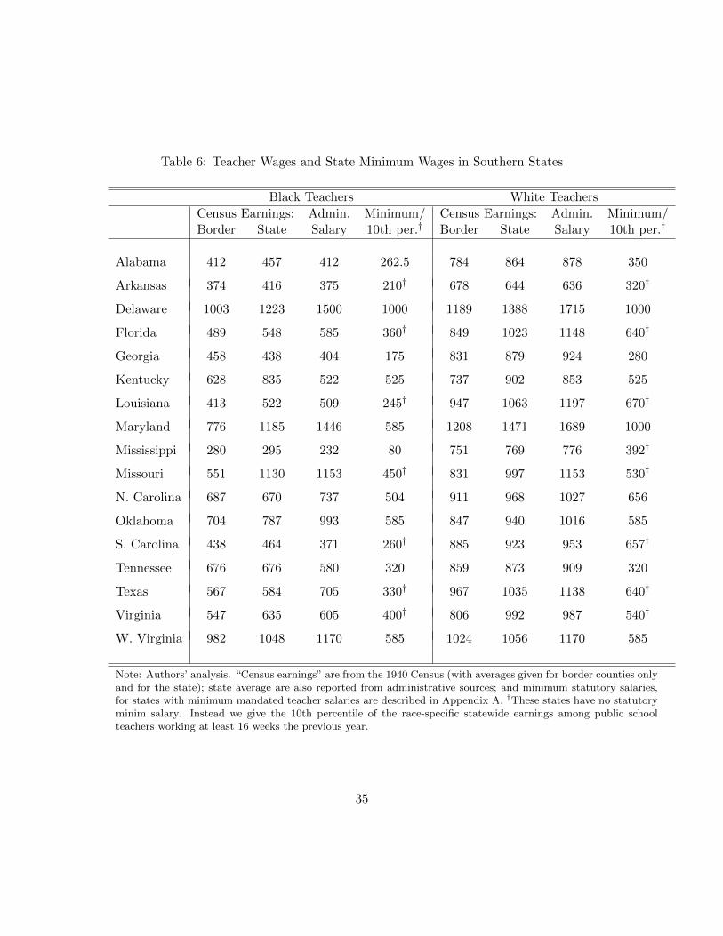
Table 6: Teacher Wages and State Minimum Wages in Southern States

Black Teachers White Teachers

Census Earnings: Admin. Minimum/ Census Earnings: Admin. Minimum/Border State Salary 10th per.† Border State Salary 10th per.†

Alabama 412 457 412 262.5 784 864 878 350

Arkansas 374 416 375 210† 678 644 636 320†

Delaware 1003 1223 1500 1000 1189 1388 1715 1000

Florida 489 548 585 360† 849 1023 1148 640†

Georgia 458 438 404 175 831 879 924 280

Kentucky 628 835 522 525 737 902 853 525

Louisiana 413 522 509 245† 947 1063 1197 670†

Maryland 776 1185 1446 585 1208 1471 1689 1000

Mississippi 280 295 232 80 751 769 776 392†

Missouri 551 1130 1153 450† 831 997 1153 530†

N. Carolina 687 670 737 504 911 968 1027 656

Oklahoma 704 787 993 585 847 940 1016 585

S. Carolina 438 464 371 260† 885 923 953 657†

Tennessee 676 676 580 320 859 873 909 320

Texas 567 584 705 330† 967 1035 1138 640†

Virginia 547 635 605 400† 806 992 987 540†

W. Virginia 982 1048 1170 585 1024 1056 1170 585

Note: Authors’ analysis. “Census earnings” are from the 1940 Census (with averages given for border counties onlyand for the state); state average are also reported from administrative sources; and minimum statutory salaries,for states with minimum mandated teacher salaries are described in Appendix A. †These states have no statutoryminim salary. Instead we give the 10th percentile of the race-specific statewide earnings among public schoolteachers working at least 16 weeks the previous year.

35

Table 7: Comparisons of Cross-Border Counties, State with the Lower Minimum Black TeacherSalary (or 10th Percentile) Listed First

State Education Mean Upward Coun- BlacksBorder of Adults Farm Urban Income Mobility ties 16–18

White Black White Black White Black

A. Borders between a Deep South State and a Peripheral South State

Alabama 7.68 4.63 0.55 0.13 619 310 0.44 0.17 4 439Florida 7.44 4.82 0.45 0.12 642 330 0.47 0.31 5 249AL-FL Gap 0.24 -0.19 0.09 0.01 -23 -20 -0.03 -0.14

Alabama 7.57 4.34 0.68 0.17 635 257 0.37 0.19 2 546Tennessee 7.77 5.31 0.72 0.12 688 351 0.40 0.21 3 271AL-TN Gap -0.20 -0.97 -0.04 0.06 -53 -94 -0.03 -0.01

Arkansas 8.72 5.08 0.63 0.14 930 332 0.51 0.22 4 970Louisiana 8.71 4.42 0.73 0.10 1004 355 0.62 0.22 5 830AR-LA Gap 0.01 0.65 -0.10 0.04 -74 -23 -0.11 -0.00

Georgia 8.10 4.15 0.51 0.14 796 319 0.49 0.21 8 508Florida 8.09 4.15 0.58 0.13 773 323 0.49 0.20 6 431GA-FL Gap 0.01 0.00 -0.07 0.01 23 -4 0.00 0.01

Louisiana 8.43 4.47 0.50 0.23 971 404 0.61 0.23 6 1096Texas 8.36 5.51 0.63 0.16 812 348 0.59 0.32 6 685LA-TX Gap 0.07 -1.04 -0.13 0.07 159 56 0.02 -0.07

Mississippi 8.58 4.14 0.88 0.00 1007 264 0.38 0.05 3 1810Arkansas 8.05 4.72 0.77 0.10 870 300 0.38 0.15 4 1241MS-AR Gap 0.53 -0.58 0.11 -0.10 137 -35 0.05 -0.10

Mississippi 8.25 5.06 0.81 0.06 480 230 0.43 0.11 5 466Tennessee 8.32 5.46 0.65 0.15 769 301 0.46 0.26 5 2031MS-TN Gap -0.07 -0.40 0.17 -0.09 -290 -72 -0.03 -0.15

S. Carolina 7.77 4.64 0.57 0.14 887 384 0.46 0.24 9 1240N. Carolina 7.84 5.12 0.61 0.13 872 405 0.54 0.33 12 749SC-NC Gap -0.06 -0.48 -0.04 0.01 15 -21 -0.08 -0.09

Note: Table continues on the next page.

36

Table 7: Comparisons of Cross-Border Counties, State with the Lower Minimum Black TeacherSalary (or 10th Percentile) Listed First—Table Continued

State Education Mean Upward Coun- BlacksBorder of Adults Farm Urban Income Mobility ties 16–18

White Black White Black White Black

B. Borders Not between a Deep South State and a Peripheral South State

Arkansas 7.73 6.06 0.62 0.09 545 373 0.42 0.28 4 141Oklahoma 7.14 5.57 0.55 0.03 509 280 0.43 0.23 2 326AR-OK Gap 0.58 0.49 0.07 0.05 36 93 0.00 0.05

Arkansas 8.53 5.36 0.54 0.29 835 354 0.49 0.21 1 608Texas 8.85 6.12 0.62 0.14 833 332 0.55 0.34 2 924AR-TX Gap -0.32 -0.76 -0.08 0.15 2 22 -0.06 -0.13

Georgia 7.78 4.56 0.57 0.21 792 351 0.47 0.21 13 453Alabama 7.54 4.50 0.69 0.12 778 295 0.40 0.17 9 593GA-AL Gap 0.24 0.06 -0.12 0.09 14 56 0.07 0.04

Georgia 8.37 4.52 0.60 0.21 865 322 0.50 0.20 11 816S. Carolina 8.61 4.30 0.64 0.07 902 299 0.55 0.18 9 978GA-SC Gap -0.25 0.22 -0.04 0.15 -37 22 -0.05 0.02

Maryland 8.09 5.67 0.40 0.16 857 455 0.60 0.51 4 333Delaware 8.90 5.66 0.48 0.15 1078 472 0.57 0.42 2 443MD-DE Gap -0.81 0.01 -0.08 0.01 -221 -17 0.03 0.09

Mississippi 8.61 5.10 0.65 0.11 627 293 0.51 0.18 8 548Alabama 7.92 4.99 0.57 0.16 693 360 0.41 0.23 6 794MS-AL Gap 0.69 0.11 0.09 -0.05 -65 -67 0.10 -0.05

Mississippi 9.14 4.74 0.74 0.12 804 307 0.53 0.13 9 638Louisiana 8.92 3.94 0.72 0.12 941 291 0.58 0.15 8 572MS-LA Gap 0.22 0.80 0.02 0.00 -137 17 -0.05 -0.02

Tennessee 7.31 5.40 0.68 0.11 619 366 0.37 0.23 11 193Kentucky 7.42 5.68 0.66 0.11 568 300 0.37 0.24 15 134TN-KY Gap -0.11 -0.27 0.02 -0.01 51 66 0.00 -0.01

Tennessee 6.94 4.12 0.63 0.00 406 236 0.25 0.02 1 171Missouri 6.96 4.94 0.70 0.00 528 281 0.35 0.18 1 415TN-MO Gap -0.02 -0.83 -0.07 0.00 -122 -46 -0.10 -0.15

Virginia 8.17 4.81 0.54 0.01 981 476 0.58 0.26 7 346Maryland 8.16 5.31 0.41 0.22 973 402 0.59 0.49 4 419VA-MD Gap 0.01 -0.51 0.14 -0.21 8 73 -0.00 -0.23

Virginia 7.47 4.54 0.75 0.04 856 383 0.46 0.21 10 779N. Carolina 8.05 5.11 0.69 0.07 938 409 0.58 0.28 11 745VA-NC Gap -0.59 -0.57 0.05 -0.03 -87 -26 -0.12 -0.06

Note: Authors’ analysis, 1940 U.S. Census. Summary statistics are displayed for border county pairs for which thedifference in the average educational attainment of whites aged 25–55 is less than one year. We list cases with at least100 black 16–18 year olds on each side of the border. “Upward mobility” is the fraction of 16–18 year olds attaining9th grade in families with parental education 5–8. 37

Table 8: Effect of Teacher Salaries on Educational Attainment among Black Children,Border County Analysis

First ReducedOLS Stage Form 2SLS F-Stat n nc

A. Effects on Years of Schooling

1. Baseline 0.285*** 0.800*** 0.265*** 0.331*** 66.8 207 28(0.057) (0.097) (0.061) (0.064)

2. Rural Areas 0.327*** 0.814*** 0.295*** 0.362*** 65.9 206 28(0.074) (0.100) (0.076) (0.080)

B. Effects on 9th Grade Attainment

1. Baseline 0.012** 0.845*** 0.012 0.014* 69.0 208 28(0.005) (0.102) (0.008) (0.009)

2. Rural Areas 0.010 0.860*** 0.016* 0.018** 66.4 207 28(0.007) (0.105) (0.008) (0.009)

Note: Author’s analysis, 1940 Census and state administrative records. The sample is restrictedto county border pairs for which the difference in the education of whites is less than one year,there are at least five black individuals aged 16–18 in each county, and at least one black teacherin each county in the 1940 Census. Our instrument is the mandated minimum salary (or the10th percentile of earnings for states with no minimum salary). Teacher salaries are measuredfrom the Census. Controls include differences between counties in high schools, Rosenwald Fundexposure, fraction urban, fraction living on farm, average black parental income and education,and average education of whites. n gives the number of border pairs; nc is the number ofborders. Standard errors (in parentheses) are clustered at the border level; ***p < 0.01,**p < 0.05, *p < 0.10.

38

Table 9: Effect of Teacher Salaries on Years of Education among White Children, BorderCounty Analysis

First ReducedOLS Stage Form 2SLS F-Stat n nc

A. Effects on Years of Schooling (Parental Education 0-4 Grades)

1. Baseline 0.149** 0.477*** 0.114** 0.238** 31.4 269 32(0.059) (0.085) (0.053) (0.110)

2. Rural Areas 0.138*** 0.483*** 0.111** 0.231** 32.3 269 32(0.059) (0.085) (0.053) (0.103)

B. Effects on Years of Schooling (Parental Education 5-8 Grades)

1. Baseline 0.098*** 0.483*** 0.054 0.112 30.1 269 32(0.033) (0.088) (0.050) (0.095)

2. Rural Areas 0.102*** 0.488*** 0.060 0.123 30.8 269 32(0.035) (0.087) (0.050) (0.092)

C. Effects on 9th Grade Attainment (Parental Education 5–8 Grades)

1. Baseline 0.009** 0.477*** 0.012** 0.027** 29.1 270 32(0.004) (0.088) (0.005) (0.010)

2. Rural Areas 0.009* 0.486*** 0.014*** 0.029*** 31.2 269 32(0.005) (0.087) (0.005) (0.010)

Note: Author’s analysis, 1940 Census. The sample is restricted to county border pairs forwhich the difference in the education of whites is less than one year. Our instrument is themandated minimum salary (or the 10th percentile of earnings for states with no minimumsalary). Teacher salaries are measured from the Census. Controls include differences betweencounties in fraction urban, fraction living on farm, average parental income of whites, andaverage education of whites. n gives the number of border pairs; nc is the number of borders.Standard errors (in parentheses) are clustered at the border level; ***p < 0.01, **p < 0.05,*p < 0.10.

39

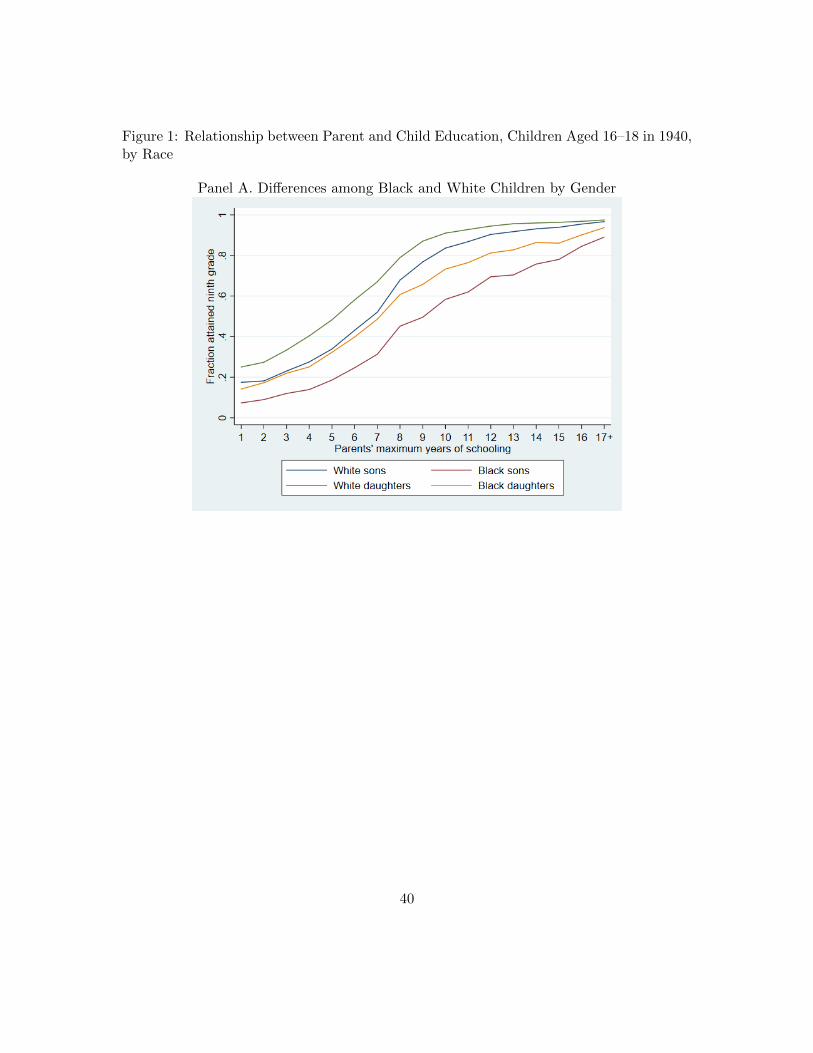
Figure 1: Relationship between Parent and Child Education, Children Aged 16–18 in 1940,by Race

Panel A. Differences among Black and White Children by Gender

40

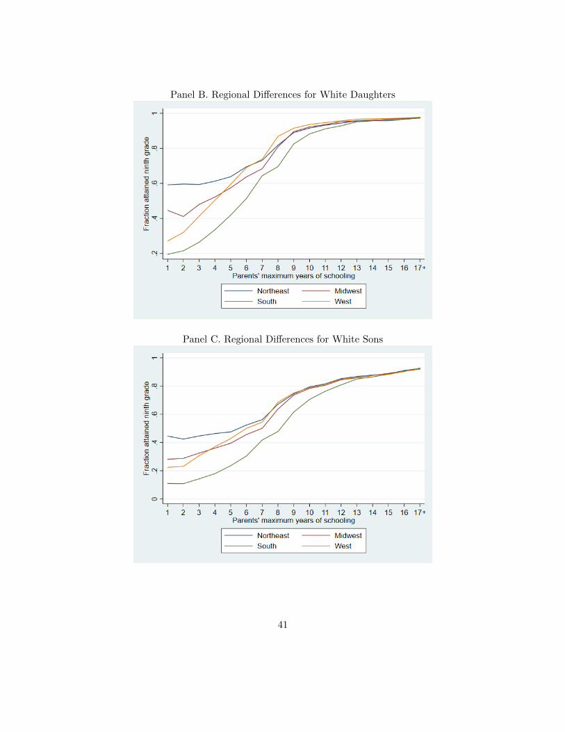
Panel B. Regional Differences for White Daughters

Panel C. Regional Differences for White Sons

41

Panel D. Racial Differences in the South for Daughters

Panel E. Racial Differences in the South for Sons

42

Panel F. Differences among Immigrant and Native-Born Families

Panel G. Differences among Immigrants by Region

43

Figure 2: Upward Mobility for Children Aged 16–18 in 1940, by Region

44

Figure 3: Proportion with 9+ Grades of Education, Children Aged 16–18 whose ParentsHave 5–8 Years of Education

Panel A. Upward Mobility for White Daughters by State

Panel B. Upward Mobility for White Sons by State

45

Panel C. Upward Mobility for Black Daughters by State

Panel D. Upward Mobility for Black Sons by States

46

Figure 4: The Geography of Upward Mobility at the County Level

A. Upward Mobility in Education, 1922-26 Birth Cohorts

B. Upward Mobility in Income, 1980-93 Birth Cohorts (Chetty et al., 2014a)

47

C. Upward Mobility in Education, 1922-26 Birth Cohorts, Black Families

D. Upward Mobility in Education, 1922-26 Birth Cohorts, White Families

48

Figure 5: Relationship between Upward Mobility in Education and School Quality Mea-sures

Panel A. White Daughters

49

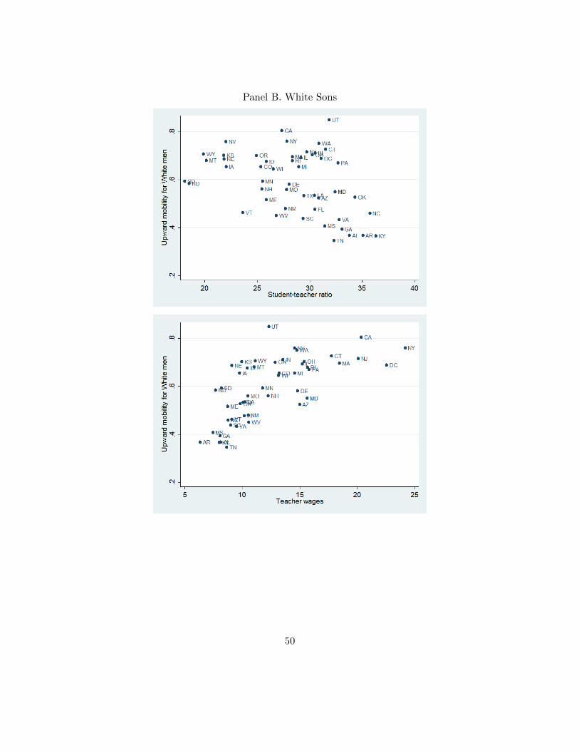
Panel B. White Sons

50

Panel C. Black Daughters in Southern States

51

Panel D. Black Sons in Southern States

52

Figure 6: Educational Choice as School Quality Increases—MR(E) Shifts Upward

MC(E)poorlyeducatedparent

������

������

�����

�����

E∗ E∗∗

MC(E)welleducatedparent

�����

������

�

������

����

12

6

ProportionalMarginal Costor Return

Education E

HHHHH

HHHHHH

HHHHHHH

HHHH

HHHH

HHHHHH

HHHHHH

HHHHHHMR(E)

53

Figure 7: Proportion of Individuals Aged 5 to 20 Living with a Parent and Enrolled inSchool

Panel A. White Daughters

Panel B. White Sons

54

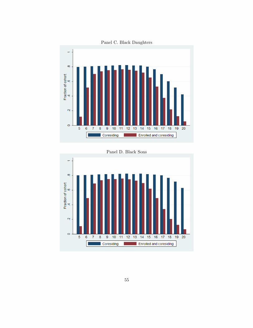
Panel C. Black Daughters

Panel D. Black Sons

55

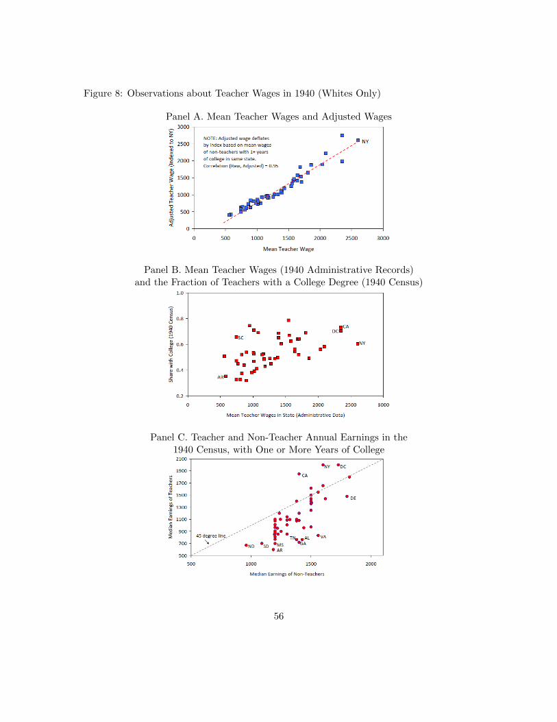
Figure 8: Observations about Teacher Wages in 1940 (Whites Only)

Panel A. Mean Teacher Wages and Adjusted Wages

Panel B. Mean Teacher Wages (1940 Administrative Records)and the Fraction of Teachers with a College Degree (1940 Census)

Panel C. Teacher and Non-Teacher Annual Earnings in the1940 Census, with One or More Years of College

56

Figure 9: Relationship between Predicted Child Education and Parental Education

Panel A. White Families

Panel B. Black Families

57

Figure 10: Border Counties Used in the County-Level Analysis

58

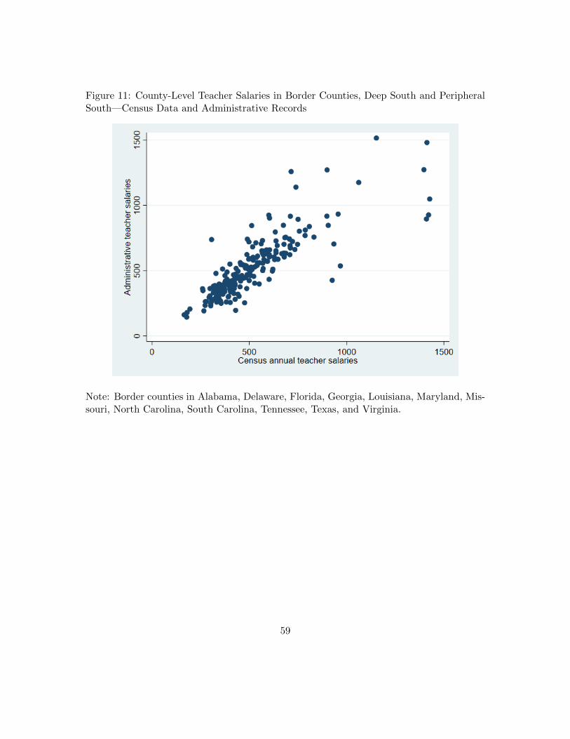
Figure 11: County-Level Teacher Salaries in Border Counties, Deep South and PeripheralSouth—Census Data and Administrative Records

Note: Border counties in Alabama, Delaware, Florida, Georgia, Louisiana, Maryland, Mis-souri, North Carolina, South Carolina, Tennessee, Texas, and Virginia.

59

Figure 12: Earnings of Teachers Relative of Non-Teachers with Similar Education, BorderCounties

60

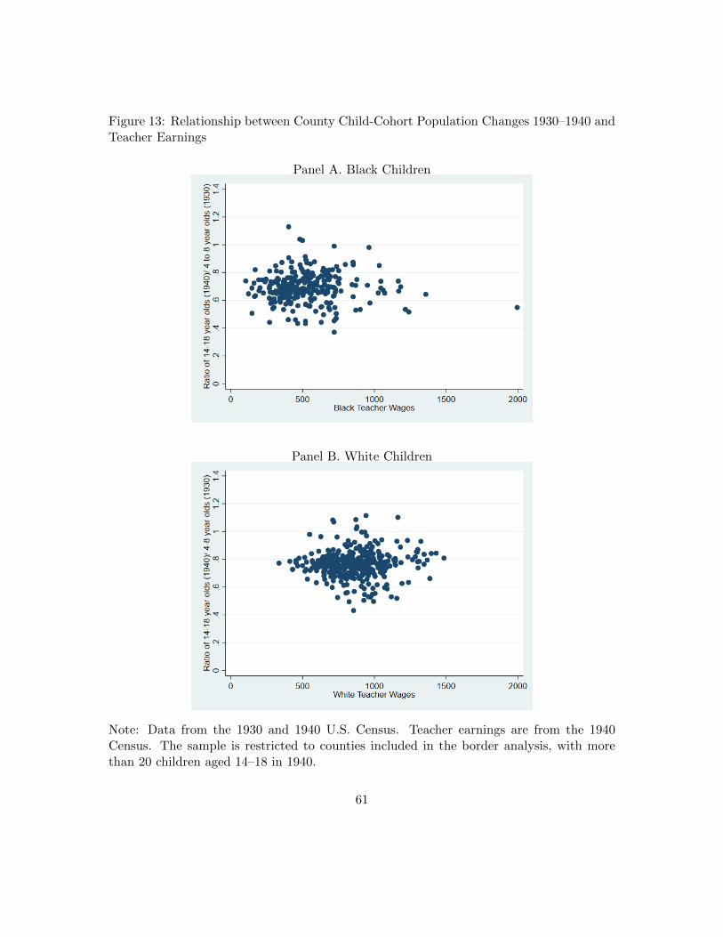
Figure 13: Relationship between County Child-Cohort Population Changes 1930–1940 andTeacher Earnings

Panel A. Black Children

Panel B. White Children

Note: Data from the 1930 and 1940 U.S. Census. Teacher earnings are from the 1940Census. The sample is restricted to counties included in the border analysis, with morethan 20 children aged 14–18 in 1940.

61

Figure 14: Relationship between Teacher Earnings and Teacher Education in SouthernBorder Counties

Panel A. Black Teachers

Panel B. White Teachers

62

References

Aakvik, Arild, Kjell Gunnar Salvanes, and Bhashkar Mazumder. 2010. “Measur-ing Heterogeneity in the Returns to Education Using an Education Reform,” EuropeanEconomic Review, 54(4): 483-500.

Aaronson, Daniel, and Bhashkar Mazumder. 2011. “The Impact of RosenwaldSchools on Black Achievement,” Journal of Political Economy, 119(5): 821-888.

Aaronson, Daniel, Bhashkar Mazumder, Seth G. Sanders and Evan J. Tay-lor. 2017. “Estimating the Effect of School Quality on Mortality in the Presence ofMigration: Evidence from the Jim Crow South,” Working Paper.

Abbott, Edith. 1908. “A Study of the Early History of Child Labor in America,”American Journal of Sociology, 14(1): 15-37.

Altonji, Joseph G., Todd E. Elder, and Christopher R. Taber. 2005. “Selection onObserved and Unobserved Variables: Assessing the Effectiveness of Catholic Schools,”Journal of Political Economy, 113(1): 151-184.

Bayer, Patrick and Kerwin K. Charles. forthcoming.“Divergent Paths: A New Per-spective on Earnings Differences Between Black and White Men Since 1940,” QuarterlyJournal of Economics.

Becker, Gary S., and Nigel Tomes. 1979. “An Equilibrium Theory of the Distributionof Income and Intergenerational Mobility,” Journal of Political Economy, 87(6): 1153-1189.

Becker, Gary S., and Nigel Tomes. 1986. “Human Capital and the Rise and Fall ofFamilies,” Journal of Labor Economics, 4(3), Part 2: S1-S39.

Benson, Charles S., and Kevin O’Halloran. 1987.“The Economic History of SchoolFinance in the United States,” Journal of Education Finance, 12(4): 495-515

Bergeron, Paul, Stephen Ash, and Jeanette Keith. 1999. Tennesseans and TheirHistory, University of Tennessee Press.

Black, Dan, Seth G. Sanders, Evan J. Taylor and Lowell J. Taylor. 2015. “TheImpact of the Great Migration on Mortality of African Americans: Evidence from theDeep South,” American Economic Review, 105(2): 477-503

Black, Sandra E., Paul J. Devereux, and Kjell G. Salvanes. 2005. “Why the AppleDoesn’t Fall Far: Understanding Intergenerational Transmission of Human Capital.”American Economic Review, 95(1): 437-449.

Black, Sandra E., and Paul J. Devereux. 2011. “Recent Developments in Inter-generational Mobility.” in Orley Ashenfelter and David Card (ed.), Handbook of LaborEconomics, volume 4. Amsterdam: North-Holland: 1487-1541.

Blau, Peter M., and Otis Dudley Duncan. 1967. The American OccupationalStructure. New York: Wiley.

Bond, Horace Mann. 1934. The Education of the Negro in the American Social Order.Octagon Books.

63

Boustan, Leah Platt. 2016. Competition in the Promised Land: Black Migrants inNorthern Cities and Labor Markets. Princeton University Press.

Card, David. 1995a. “Earnings, Schooling and Ability Revisited,” in Solomon Polachek,ed., Research in Labor Economics, Vol. 14. JAI Press, Greenwich, CT: 23-48.

Card, David. 1995b. “Using Geographic Variation in College Proximity to Estimate theReturn to Schooling,” in Louis N. Christofides, E. Kenneth Grant, and Robert Swidin-sky, eds., Aspects of Labour Market Behaviour: Essays in Honour of John Vanderkamp.University of Toronto Press, Toronto, Canada: 201-222.

Card, David. 1999. “The Causal Effect of Education on Earnings,” in Orley Ashenfelterand David Card (ed.), Handbook of Labor Economics, volume 3. Amsterdam: North-Holland: 1801-1863.

Card, David. 2001. “Estimating the Return to Schooling: Progress on Some PersistentEconometric Problems,” Econometrica, 69(5): 1127-1160.

Card, David, John E. DiNardo, and Eugena Estes. 2000. “The More ThingsChange: Immigrants and the Children of Immigrants in the 1940s, the 1970s, and the1990s,” in George Borjas, editor, Issues in the Economics of Immigration. Chicago:University of Chicago Press for the NBER.

Card, David, and Alan B. Krueger. 1992a. “Does School Quality Matter? Returnsto Education and the Characteristics of Public Schools in the United States,” Journalof Political Economy, 100(1): 1-40.

Card, David, and Alan B. Krueger. 1992b.“School Quality and Black-White RelativeEarnings: A Direct Assessment,” Quarterly Journal of Economics, 107(1): 151-200.

Card, David and Alan B. Krueger. 1996. “School Resources and Student Outcomes:An Overview of the Literature and New Evidence from North and South Carolina,”Journal of Economic Perspectives, 10(4), 31-50.

Carneiro, Pedro, Italo Garcia, Kjell Salvanes, Emma Tominey. 2015. “Intergen-erational Mobility and the Timing of Parental Income,” Working Paper.

Carruthers, Celeste and Marianne H. Wanamaker. 2013. “Closing the Gap? TheEffect of Private Philanthropy on the Provision of African-American Schooling in theU.S. South,” Journal of Public Economics, 101: 53-67.

Clay, Karen, Jeff Lingwall, and Melvin Stephens Jr. 2012. “Do Schooling LawsMatter? Evidence from the Introduction of Compulsory Attendance Laws in the UnitedStates,” NBER Working Paper No. 18477.

Chetty, Raj, Nathaniel Hendren, Patrick Kline, and Emmanuel Saez. 2014a.“Where is the Land of Opportunity? The Geography of Intergenerational Mobility inthe United States,” Quarterly Journal of Economics, 129(4): 1553-1623.

Chetty, Raj, Nathaniel Hendren, Patrick Kline, Emmanuel Saez, and NickTurner. 2014b. “Is the United States Still a Land of Opportunity? Recent Trendsin Intergenerational Mobility,” American Economic Review Papers and Proceedings,104(5): 141-147.

Chetty, Raj Chetty and Nathaniel Hendren. 2016a. “The Effects of Neighborhoods

64

on Intergenerational Mobility I: Childhood Exposure Effects,” NBER Working PaperNo. 23,001.

Chetty, Raj Chetty and Nathaniel Hendren. 2016b. “The Impacts of Neigh-borhoods on Intergenerational Mobility II: County-Level Estimates.” NBER WorkingPaper No. 23,002.

Chetty, Raj, Nathaniel Hendren, Maggie R. Jones, and Sonya R. Porter.2018. “Race and Economic Opportunity in the United States: An IntergenerationalPerspective,” NBER Working Paper No. 24,441.

Coen-Pirani, Daniele and Michael Wooley. 2018. “Fiscal Centralization: Theoryand Evidence from the Great Depression,” American Economic Journal: EconomicPolicy, 10(2): 39-61.

Coleman, Ada. 1947. “The Salary Equalization Movement,” Journal of Negro Educa-tion, 16(2): 235-241.

Coleman, James S., et al. 1966. Equality of Educational Opportunity. Washington:Government Printing Office.

Davis, Harwell G., editor. 1927. Alabama School Code. Department of Education,State of Alabama.

Donohue, John, James Heckman, and Petra Todd. 2002. “The Schooling ofSouthern Blacks: The Roles of Legal Activism and Private Philanthropy, 1910–1960,”Quarterly Journal of Economics, 117(1): 225-68.

Dube, Arindrajit, William T. Lester and Michael Reich. 2010. “Minimum WageEffects across State Borders: Estimates Using Contiguous Counties,” Review of Eco-nomics and Statistics, 92(4): 945-964

Education, A. D., United States Bicentennial Intern Program in EducationAlabama Pilot Project, and Board, S. R. (n. d.). 1975. “History of Educationin Alabama.”

Eichenlaub, Suzanne C., Stuart E. Tolnay, and J. Trent Alexander. 2010.“Moving Out but Not Up: Economic Outcomes in the Great Migration,” AmericanSociological Review, 75(1): 10125.

Fitzgerald, Stephanie. 2007. The Scopes Trial: The Battle Over Teaching Evolution,Compass Point Books.

Galton, Francis. 1869. Hereditary Genius: An Inquiry into its Laws and Consequences,London: Macmillan.

Goldin, Claudia. 1998. “America’s Graduation from High School: The Evolutionand Spread of Secondary Schooling in the Twentieth Century,” Journal of EconomicHistory, 58(2): 345-374.

Goldin, Claudia. 2001. “The Human-Capital Century and American Leadership:Virtues of the Past,” Journal of Economic History, 61(2): 263-292.

Goldin, Claudia, and Lawrence F. Katz. 1998. “The Origins of State-Level Differ-ences in the Public Provision of Higher Education: 1890–1940,” American EconomicReview, 88(2): 303-308.

65

Goldin, Claudia, and Lawrence F. Katz. 1999. “Human Capital and Social Capital:The Rise of Secondary Schooling in America, 1910–1940,” Journal of InterdisciplinaryHistory, 29(4): 683-723.

Goldin, Claudia and Lawrence Katz. 2008. The Race between Education and Tech-nology. Cambridge, MA: The Belknap Press of Harvard University Press.

Hanushek, Eric A. 1974. “Efficient Estimators for Regressing Regression Coefficients,”The American Statistician, 28(2): 66-67.

Hanushek, Eric A., Steven G. Rivkin, and Lori L. Taylor. 1996. “Aggregationand the Estimated Effects of School Resources,” Review of Economics and Statistics,78(4): 611-27.

Hilger, Nathaniel G. 2017a. “Upward Mobility and Discrimination: the Case of Asian-Americans,” Working Paper, Brown University.

Hilger, Nathaniel G. 2017b. “ The Great Escape: Intergenerational Mobility in theUnited States, 1930–2010,” Working Paper, Brown University.

Jencks, Christopher. 1972. Inequality: A Reassessment of the Effect of Family andSchooling in America. New York: Basic Books.

Jones, Eugene K. 1928. “Social Work Among Negroes,” Annals of the AmericanAcademy of Political and Social Science, 130: 287-293.

Knox, Ellis O. 1954. “Racial Integration in the Public Schools of Arizona, Kansas andNew Mexico,” Journal of Negro Education, 23(3): 290-295.

Kuo, Joyce. 1998. “Excluded, Segregated and Forgotten: A Historical View of theDiscrimination of Chinese Americans in Public Schools,” Asian American Law Journal,5(7): 181-212.

Lleras-Muney, Adriana. 2002. “Were Compulsory Education and Child Labor LawsEffective? An Analysis from 1915 to 1939 in the U.S.” Journal of Law and Economics,45(2): 401-435.

Loury, Glenn C. 1981. “Intergenerational Transfers and the Distribution of Earnings,”Econometrica, 49(4): 843-867.

Lundborg, Petter, Anton Nillson and Dan-Olof Rooth. 2014. “Parental Educationand Offspring Outcomes: Evidence from the Swedish Compulsory School Reform,”American Economic Journal: Applied Economics, 6(1): 253-278

Maloney, Thomas N. 1994. “Wage Compression and Wage Inequality between Blackand White Males in the United States, 1940–1960,” Journal of Economic History, 54(2): 358-81.

Margo, Robert A. 1985. Disfranchisement, School Finance, and the Economics ofSegregated Schools in the United States South, 1890-1910. New York: Garland Press.

Margo, Robert A. 1986. “Race, Educational Attainment, and the 1940 Census,” Journalof Economic History, 46(1): 189-198.

Margo, Robert A. 1990. Race and Schooling in the South, 1880–1950: An EconomicHistory. Chicago: University of Chicago Press.

66

Margo, Robert A. 1995. “Explaining Black-White Wage Convergence, 1940–1950,”Industrial and Labor Relations Review, 48(3): 470-481.

Mazumder, Bhashkar, 2005. “Fortunate Sons: New Estimates of IntergenerationalMobility in the U.S. using Social Security Earnings Data,” Review of Economics andStatistics, 87(2): 235-255.

Meghir, Costas and Martin Palme. 2005. “Educational Reform, Ability and ParentalBackground,” American Economic Review, 95(1): 414-424.

Meghir, Costas, and Pierre-Andre Chiappori. 2014. “Intrahousehold Inequality,”NBER Working Paper No. 20,191.

Meghir, Costas, Marten Palme, and Emilia Simeonova. 2013. “Education,Cognition and Health: Evidence from a Social Experiment,” NBER Working PaperNo. 19,002.

Mincer, Jacob. 1958. “Investment in Human Capital and Personal Income Distribu-tion,” Journal of Political Economy, 66(4): 281-302.

Miller, Herman P., and Leon R. Paley. 1958. “Income Reported in the 1950Census and on Income Tax Returns,” in An Appraisal of the 1950 Census IncomeData. Princeton University Press.

Mulligan, Casey B. 1999. “Galton versus the Human Capital Approach to Inheritance,”Journal of Political Economy, 107(S6): S184-S224.

National Education Association of the United States. 1940. State Minimum-SalaryStandards for Teachers, Washington, D.C.

North Carolina, Department of Justice. 1922. Biennial Report of the Attorney-General of the State of North Carolina. Raleigh: Edwards & Broughton and E. M. Uzzell,State Printers.

Oster, Emily. 2017. “Unobservable Selection and Coefficient Stability: Theory andEvidence,” Journal of Business and Economic Statistics, 1-18.

Peterson, Gladys T. 1935. “The Present Status of the Negro Separate School as Definedby Court Decisions.” Journal of Negro Education, 4(3): 351-374.

Ruggles, Steven, J. Trent Alexander, Katie Genadek, Ronald Goeken, MatthewB. Schroeder, and Matthew Sobek. 2010. Integrated Public Use Microdata Series:Version 5.0. Machine-Readable Database. Minneapolis: University of Minnesota.

Shiver, Lee A. 1983. “A Historical Review of the Development of Florida’s SchoolFinance Plan and the Fiscal Equalization Effects of the Florida Education FinanceProgram,” Ph.D. Dissertation, University of Florida.

Smith, James P., and Finis R. Welch. 1989. “Black Economic Progress after Myrdal,”Journal of Economic Literature, 27(2): 519-564.

Snyder, Thomas D. 1993. 120 Years of American Education: A Statistical Portrait.Washington, D.C.: U.S. Department of Education, Office of Educational Research andImprovement, National Center for Education Statistics.

Solon, Gary. 1992. “Intergenerational Income Mobility in the United States,” AmericanEconomic Review, 82(3): 393-408.

67

Solon, Gary. 1999.“Intergenerational Mobility in the Labor Market,” in Orley Ashen-felter and David Card (ed.), Handbook of Labor Economics, volume 3, Amsterdam:North-Holland: 1761-1800.

South Carolina, State Department of Education. 1938. Annual Report of the StateSuperintendent of Education of the State of South Carolina, volume 70-71.

Trow, Martin. 1961. “The Second Transformation of American Secondary Education,”International Journal of Comparative Sociology, 2(2): 144-166.

United States Census Bureau. 1975. Historical Statistics of the United States, Colo-nial Times to 1970. Washington, D.C.

United States Census Bureau. 2010. County Adjacency File. https://www.census.gov/geo/reference/county-adjacency.html

Wallis, John Joseph. 2000. “American Government Finance in the Long Run: 1790 to1990,” Journal of Economic Perspectives, 14(1): 61-82.

Wilson, Charles H. 1947. Education for Negroes in Mississippi since 1910. Boston,MA: Meador.

Wollenberg, Charles. 1974. “Mendez v.Westminster: Race, Nationality and Segrega-tion in California Schools.” California Historical Quarterly 53:317-332.

Wollenberg, Charles. 1995. “The Yellow Peril in School,” in D. Nakanishi andT. Yamano-Nishida (ed.), The Asian-American Educational Experience: A Source Bookfor Teacher and Students, New York: Routledge.

Wright, Richard. 1941. 12 Million Black Voices: A Folk History of the Negro in theUnited States, New York: Viking.

68