the long-term price-earnings ratio - ka536/long-term pe.pdf · the long-term price earnings ratio...

Journal of Business Finance & Accounting, 33(7) & (8), 1063–1086, September/October 2006, 0306-686Xdoi: 10.1111/j.1468-5957.2006.00621.x

The Long-Term Price-Earnings Ratio

Keith Anderson and Chris Brooks∗

Abstract: The price-earnings effect has been thoroughly documented and is the subject ofnumerous academic studies. However, in existing research it has almost exclusively beencalculated on the basis of the previous year’s earnings. We show that the power of the effecthas until now been seriously underestimated due to taking too short-term a view of earnings.Looking at all UK companies since 1975, using the traditional P/E ratio we find the differencein average annual returns between the value and glamour deciles to be 6%. This is similar toother authors’ findings. We are able to almost double the value premium by calculating the P/Eratio using earnings averaged over the previous eight years.

Keywords: price-earnings ratio, value premium, arbitrage trading rule, UK stock returns,contrarian investment

1. INTRODUCTION

The ratios of a stock’s current price to its earnings over the last company year (historicalP/E) and to analysts’ consensus forecast earnings for this year (prospective P/E) arewidely quoted statistics. The price-earnings effect was the earliest described asset pricing‘anomaly’ even before the capital asset pricing model (CAPM) itself was formulatedby Sharpe (1964). A large body of academic work has demonstrated the effect andhas attempted to decide whether it is real or a proxy for other factors.1 The firststudy demonstrating the P/E effect was by Nicholson (1960), who concluded that ‘Thepurchaser of common stocks may logically seek the greater productivity representedby stocks with low rather than high price-earnings ratios.’ Basu (1975) and (1977)generally confirmed Nicholson’s results.

The PE effect has defied rational explanation. Ball (1978), while conceding theapparent existence of such effects, considered various possible explanations for this

* The authors are respectively from the ICMA Centre, University of Reading and Cass Business School, CityUniversity. The authors would like to thank an anonymous referee for very helpful comments on a previousversion of this paper; the usual disclaimer applies. (Paper received May 2005, revised version accepted January2006. Online publication June 2006)

Address for correspondence: Chris Brooks, Faculty of Finance, Cass Business School, City University, 106Bunhill Row, London EC1Y 8TZ, UK.e-mail: [email protected]

1 See, for example, Nicholson (1960 and 1968), Basu (1975 and 1977), Ball (1978 and 1992), Jaffe, Keimand Westerfield (1989), Fuller, Huberts and Levinson (1993), Lakonishok et al. (1994) and Dreman (1998)to mention just US studies.

C© 2006 The AuthorsJournal compilation C© 2006 Blackwell Publishing Ltd, 9600 Garsington Road, Oxford OX4 2DQ, UKand 350 Main Street, Malden, MA 02148, USA. 1063

1064 ANDERSON AND BROOKS

anomaly, including systematic experimental error, transaction and processing costs,and a failure of Sharpe’s two-parameter CAPM model. Fuller, Huberts and Levinson(1993) re-examined Ball’s (1978) argument by using a comprehensive multi-factormodel that allowed for systematic risk (beta), 55 industry classification factors and 13other explanatory factors for ‘risk’ such as earnings variability, leverage and foreignincome. They again found higher returns for low P/E stocks from 1973–1990, but thefactors included in the model did not account for the superior low P/E returns.

Banz and Breen (1986) criticised previous studies into the size and P/E effectsas suffering from two major biases: ex-post-selection bias and look-ahead bias. Theyeliminated these factors by amassing their own database from the COMPUSTAT tapesfor 1974–81 that accurately reflected the companies in existence and the data availableto investors at that time. Their conclusion was that although a company size effectpersisted, the P/E effect was no longer significant, i.e. that the data biases had createdthe apparent P/E effect. Jaffe, Keim and Westerfield (1989) considered the Januaryeffect as well as the size and P/E effects. They found that the conflicting results ofearlier studies could be ascribed to time-variation in the power of the different effects.

Lakonishok, Schleifer and Vishny (1994) (‘LSV’ hereafter) defined value strategiesas buying shares with low prices compared to some indicator of fundamental valuesuch as earnings, book value, dividends or cash flow. They divided firms into ‘value’or ‘glamour’ stocks on the basis of past growth in sales and expected future growthas implied by the current P/E ratio. LSV argued that value strategies provide higherreturns because they exploit the sub-optimal behaviour of investors. They found little,if any, support for the view that value strategies were fundamentally riskier. Value stocksoutperformed glamour stocks quite consistently, yielding particularly strong abnormalreturns during market downturns. However, Fama and French (1993 and 1996) foundthat value stock anomalies could be successfully explained by a three-factor modelinvolving market returns, size and book to market value. But unlike the CAPM, therewas no theoretical underpinning offered as to why these factors and not others shouldbe important.

The P/E effect has been observed in many stock markets,2 although there areconsiderably fewer studies investigating the existence and possible justifications fora value effect in the UK. Levis (1989) was the first such study, finding strong resultsin favour of a value premium. Levis and Liodakis (2001) focused on ascribing thesource of the value anomaly to either investors’ naive extrapolations of past sales andearnings growth, as put forward by LSV, or to systematic errors in analysts’ forecasts oflong-term growth. They used data on 3,131 non-financial companies with only a singleclass of share between 1968 and 1997. By looking at EPS growth for five years bothbefore and after portfolio formation, they showed that companies in the lowest P/Edecile experienced low EPS growth over the five years prior to portfolio formation butimproved growth thereafter. EPS growth exhibited mean reversion. Thus the anomaliescould be ascribed to prior losers becoming winners and vice-versa, as suggested byDe Bondt and Thaler (1985). However the pattern of growth did not fit the naive

2 In addition to the above research, countries for which P/E effect studies have been carried out include:thirteen countries around the world (Fama and French, 1998); the UK (Levis, 1989; Gregory et al., 2001;and Levis and Liodakis, 2001); the UK and several European countries together (Brouwer et al., 1997; andBird and Whitaker, 2003); Holland (Doeswijk, 1997); Finland (Booth et al., 1994); Japan (Aggarwal et al.,1990; Chan et al., 1991; Cai, 1997; and Park and Lee, 2003); Taiwan (Chou and Johnson, 1990); New Zealand(Chin et al., 2002).

C© 2006 The AuthorsJournal compilation C© Blackwell Publishing Ltd. 2006

THE LONG-TERM PRICE EARNINGS RATIO 1065

extrapolation hypothesis of LSV. Instead, Levis and Liodakis used I/B/E/S earningsforecast data to show that positive surprises have a large effect on value stocks and asmall effect on glamour stocks, and vice-versa for negative surprises.

Previous research has, to the best of our knowledge, always used the same approach tocalculating the E/P (the inverse of the P/E ratio): the previous year’s earnings, dividedby the share price at the time of portfolio formation. However, there is no reasonwhy only earnings from the previous year should be relevant in valuing companies.As Campbell and Shiller (1988) state, annual earnings are quite noisy as a measure offundamental value. The concept of ‘value’ may well be better captured by focusing onpermanent rather than transient earnings. We have been unable to find any previousacademic research into whether knowledge of earnings of previous years will improvethe ability of the P/E ratio to predict future returns on individual shares. Graham andDodd (1934, p.452) recommended the use of average earnings over a period of at leastfive years and preferably over seven to ten years, to give the analyst a more reliable viewof the true value of a company. Yet their conjecture does not seem to have been testedby any academic research. Campbell and Shiller (1988) and Shiller (2000) appear tobe the only existing investigations into the value of multi-year earnings averages. Theyexamined earnings over the stock index as a whole, however, rather than at the levelof individual companies with reference to the P/E effect.

We find that adding more years of earnings history increases the power of the P/Eratio to predict returns, although this does not happen monotonically. Using eight yearsof earnings rather than one, the difference between the returns of the glamour andvalue deciles is almost doubled. The simplest approach to enhancing the usefulnessof the E/P ratio is to assign stocks to value and glamour portfolios using earningsaveraged over two to eight years. However, equal weights are not necessarily optimal informing a P/E statistic that is the most efficient predictor of returns. We investigate somealternative and intuitive weighting systems. We also calculate the predictive value ofindividual past years of returns. The best weighting we find is from adding the earningsfrom last year to the earnings from eight years ago and ignoring the intervening sixyears. This is perhaps due to the low correlation between the earnings from these twoyears. Our search is, however, not exhaustive.

Finally, we attempt to deal with three possible criticisms of our approach. Usingweights derived from a regression across our whole time period may fairly be criticisedas suffering from a look-ahead bias. In order to investigate whether our results wouldbe robust to the use of different years or using a different number of years ofdata, we employ rolling five-year periods. We find that our optimum weighting, orsomething very similar, has been the optimum over most five-year periods during thepast twenty years. We also calculate the effect of bid-ask spreads on returns and show thattransactions costs can only account for a small proportion of the difference in returnsbetween the value and glamour deciles. Finally, we investigate whether the trades oftypical investors would cause liquidity problems for small company shares.

The remainder of this paper proceeds as follows. Section 2 describes the methodol-ogy employed in the calculations of long-term P/E ratios and decile portfolio returns.Section 3 presents the decile returns using the different lengths of earnings histories,where the past years of earnings are all equally weighted. Section 4 uses t-tests, standarddeviations and Sharpe ratios to examine the significance of the differences in returns.Section 5 investigates the usefulness of various weighting schemes for the past earningsfigures. Section 6 calculates the effects of the bid-ask spread on decile returns and



further examines the riskiness of long-value-short-glamour strategies. It also considerswhether the stocks involved are likely to be sufficiently liquid. Section 7 presents aportfolio illustration. Section 8 concludes.

2. DATA SOURCES AND METHODOLOGY

Initially, we collated a list of companies from the London Business School’s ‘LondonShare Price Database’ (LSPD) for the period 1975 to 2003. The LSPD holds datacommencing in 1955, but only a sample of one-third of companies is held until 1975.Thereafter, data are held for every UK listed company. We therefore only employ datafrom 1975. We excluded financial sector companies including investment trusts andcompanies with more than one type of share - for instance, voting and non-voting shares.Apportioning the earnings between the different share types would be problematic.

Earnings data are available on LSPD, but only for the previous financial year. Wetherefore used Datastream to collect all other series, as this service is able to providetime series data on most of the statistics it covers, including earnings. A four-monthgap is allowed between the year of earnings being studied and portfolio formation, toensure that all earnings data used would have been available at the time. We therefore re-quested for each company as at 1 May in each year 1975–2003, normalised earnings forthe past eight years, the current price and the returns index on that date and a year later.

A common criticism of academic studies of stock returns is that the reported returnscould not actually have been achieved in reality, due to the presence of very smallcompanies or highly illiquid shares. In an attempt at least to avoid the worst examples,we excluded companies if the share mid-price was less than 5p. We also excluded thelowest 5% of shares by market capitalisation in each year. We checked whether thisremoval of ‘micro-cap’ and penny shares had a significant effect on returns. Pennyshares and micro-caps did indeed contribute to returns, although this contribution wasacross all deciles, not just for value shares. Average returns were 1–1.5% higher when allcompanies are included, across all deciles and holding periods. An arbitrage strategythat is long in value companies and short in glamour companies would therefore belargely unaffected by the exclusion of very small companies and of penny shares. InSection 7 we also examine the impact of transactions costs, which are likely to be largerfor small firms. A further criticism of many studies is that they do not deal appropriatelywith bankruptcies. Companies that failed (i.e. were bankrupted) during the year areflagged in the LSPD. In such cases, we set the price manually to zero, as in Datastreamit often becomes fixed at the last traded price. We thus assumed a 100% loss of theinvestment in that company in such cases.

We calculated up to eight E/P statistics for each company/year return, by dividingthe sum of the earnings over the previous one to eight years by the current stock price:

EPni =

n∑

j=1EPSi j

nPi(1)

where EPSij is the normalised earnings per share for company i for j years ago, Pi is thecurrent price of company i and n is the number of years of earnings used in the EPncalculation. As earnings would be expected to rise on average over time with inflation,there is a small implicit weighting of the later earnings in favour of the earlier ones,in cases where more than one year of earnings is used. Where Datastream reported



a company as having a zero EPS, i.e. normalised earnings were negative, or there wasno EPS recorded for one or more previous years, EPn for those year(s) could notbe calculated.3 We therefore had to exclude the company from further analysis forthat EPn. Due to these factors, the number of companies for each EPn calculationgradually reduces as the EPS figure becomes unavailable for years further into the past,from 40,000 initially to 16,000 that have a full eight years of positive earnings history.

We then sorted shares by EPn, grouped them into deciles within each year andcalculated the returns for each decile for the subsequent year as if it were anindependent portfolio. In fact we calculated returns for holding periods of up to eightyears, but the results are usually qualitatively unaltered from those for one-year returnsso in most cases we do not report them. Where we used a weighted average of pastearnings, the E/P for the ith company/year return was calculated as:

EPi =

8∑

j=1Wt j EPSi j

Pi

8∑

j=1Wt j

(2)

where Wtj is the weight for the earnings for the j th year and EPSij is the normalisedearnings per share for company/year return i from individual past year j (one to eightyears previously). The right-hand side is thus a weighted average of the past eightyears of earnings divided by the current share price. The weights vary according to theweighting scheme and are explained in Section 3.

Section 6 considers the effect of the bid-ask spread on the decile returns. Bid andask prices were first recorded on Datastream in 1987 but for the majority of companiesare only available from 1991. Where the actual bid-ask spread was available for thatcompany on that day we used it, calculating the returns after allowing for spread losses.To cater for companies for which bid and ask prices were not available, we dividedcompanies into 20 categories by market capitalisation within each year and calculatedthe average bid-ask spread for each category. Companies for which bid-ask spreads werenot available then used the average bid-ask spread for their category. We applied notransaction cost where a share remained in a particular decile portfolio for more thanone year, since selling and re-purchasing the share would be unnecessary.

3. RETURNS FOR THE LONG-TERM P/E RATIO

In this section we report the main initial results of the investigation, showing theaverage portfolio returns by P/E decile. We present the results first in Table 1,showing the distribution of returns after using the EP1–EP8 statistics (i.e. based on1-8 years of earnings history) to sort companies into decile portfolios. The differencein returns does increase as one takes more years of past earnings into account, butnot monotonically: in particular there is a dip for EP2 and EP3, so that calculatingP/E ratios using the previous two or three years of earnings is less rewarding thanusing only the previous year’s earnings. This is reminiscent of the pattern of reversals

3 Unfortunately, Datastream records any zero or negative normalised earnings as zero, and there is thereforeno way to distinguish between the two.



Table 1One-Year Average Returns for Decile Portfolios, 1975–2003

EP1 % EP2 % EP3 % EP4 % EP5 % EP6 % EP7 % EP8 %

Panel A: Using All Available DataHighest P/E 18.28 18.20 18.62 16.65 17.84 17.83 18.15 16.26Decile 2 19.25 19.36 16.41 17.98 16.94 17.42 16.16 16.71Decile 3 18.38 17.32 18.92 18.68 17.78 17.51 17.05 16.43Decile 4 16.44 18.96 19.45 18.42 19.49 17.81 18.61 18.42Decile 5 17.96 18.06 17.73 18.58 17.62 19.11 18.34 19.54Decile 6 18.53 18.73 19.32 18.98 19.97 19.69 19.81 19.81Decile 7 21.59 19.53 19.86 20.77 19.61 20.18 19.86 19.39Decile 8 20.86 20.55 21.33 22.11 21.81 20.42 20.58 21.11Decile 9 22.47 21.75 22.00 22.08 22.48 22.88 22.48 23.05Lowest P/E 24.26 22.82 21.89 22.18 24.27 25.51 27.57 27.87D10 – D1 5.98 4.62 3.28 5.52 6.44 7.67 9.42 11.62

Panel B: Using Only Companies That Have a Full Eight Years of Positive EarningsHighest P/E 18.03 18.52 19.31 17.96 17.72 16.79 17.20 16.26Decile 2 19.18 17.42 16.06 16.49 15.70 15.86 15.96 16.71Decile 3 18.05 18.60 18.20 18.96 17.72 17.75 17.29 16.43Decile 4 15.26 17.25 18.23 17.58 17.96 18.17 18.25 18.42Decile 5 19.56 19.16 18.64 18.53 18.48 19.42 18.10 19.54Decile 6 18.01 19.51 19.35 18.91 19.73 20.03 20.19 19.81Decile 7 19.72 19.78 20.53 20.59 20.12 19.95 19.91 19.39Decile 8 20.28 21.33 20.81 21.03 21.27 19.77 21.10 21.11Decile 9 24.11 21.07 21.48 22.64 23.59 23.70 23.16 23.05Lowest P/E 26.34 25.93 25.94 25.92 26.28 27.14 27.44 27.87D10 – D1 8.31 7.41 6.63 7.96 8.56 10.35 10.24 11.62

Note:Companies are assigned to portfolios using statistics EP1 (the inverse of the usual P/E ratio) through toEP8 (the sum of normalised earnings over the last eight years, divided by the current share price).

identified by De Bondt and Thaler (1985), who noted an initial underperformance oftheir loser portfolios, but outperformance in years two and three. In the current case,high earnings two and three years ago tend to indicate poorer performance in thefuture. The value premium when using four or five years of earnings is quite similarto that obtained using only the previous year’s earnings, but the superiority of usingsix years or more is clear. Using a full eight years of past earnings, which is the cut-offpoint for our database, gives a value premium almost twice that of EP1.

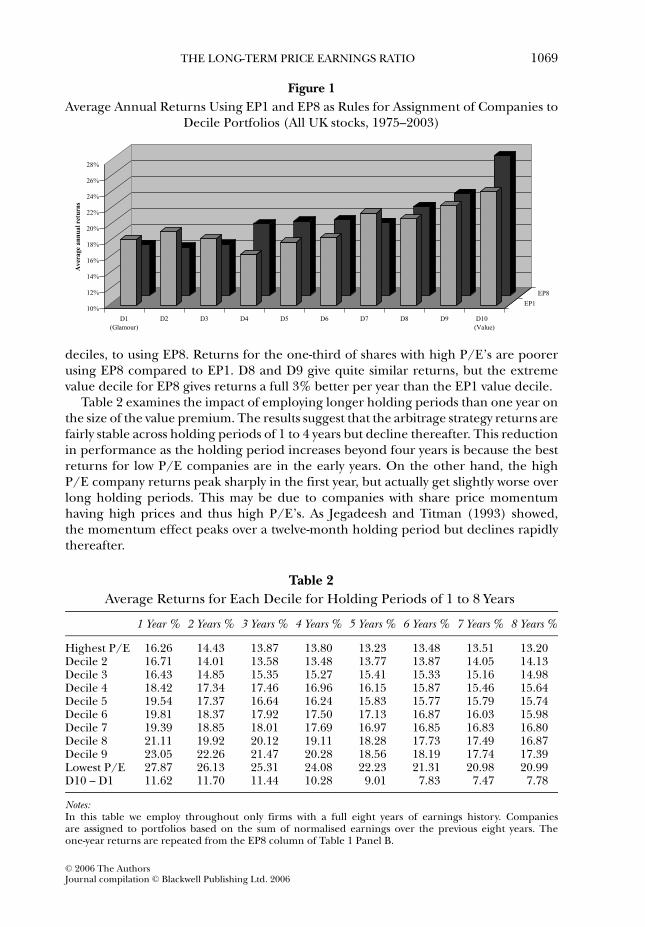
Panel A of Table 1 uses all the available company/year returns to compute theEP. This results in the number of companies included in the deciles decreasingmonotonically from left to right across the table, as we require an increasing numberof years of earnings history to compute the EP. In order to ensure that the resultsare comparable across EPn for n = 1,8, we recomputed the EPn in Panel B of Table1 using only firms with a full eight years of earnings history throughout.4 Requiringfirms to have a full eight years of earnings history leads to higher returns for the valuedecile but little change in the returns for the growth decile, so that the long-value-short-growth arbitrage strategy returns are increased by around 2-3% for EP1 through to EP7.Figure 1 compares the returns using EP1 as the basis of assignment of companies to

4 The results for EP8 are therefore identical across Panels A and B of Table 1.



Figure 1Average Annual Returns Using EP1 and EP8 as Rules for Assignment of Companies to

Decile Portfolios (All UK stocks, 1975–2003)

10%

12%

14%

16%

18%

20%

22%

24%

26%

28%

Ave

rage

ann

ual r

etur

ns

D1(Glamour)

D2 D3 D4 D5 D6 D7 D8 D9 D10 (Value)

EP1

EP8

deciles, to using EP8. Returns for the one-third of shares with high P/E’s are poorerusing EP8 compared to EP1. D8 and D9 give quite similar returns, but the extremevalue decile for EP8 gives returns a full 3% better per year than the EP1 value decile.

Table 2 examines the impact of employing longer holding periods than one year onthe size of the value premium. The results suggest that the arbitrage strategy returns arefairly stable across holding periods of 1 to 4 years but decline thereafter. This reductionin performance as the holding period increases beyond four years is because the bestreturns for low P/E companies are in the early years. On the other hand, the highP/E company returns peak sharply in the first year, but actually get slightly worse overlong holding periods. This may be due to companies with share price momentumhaving high prices and thus high P/E’s. As Jegadeesh and Titman (1993) showed,the momentum effect peaks over a twelve-month holding period but declines rapidlythereafter.

Table 2Average Returns for Each Decile for Holding Periods of 1 to 8 Years

1 Year % 2 Years % 3 Years % 4 Years % 5 Years % 6 Years % 7 Years % 8 Years %

Highest P/E 16.26 14.43 13.87 13.80 13.23 13.48 13.51 13.20Decile 2 16.71 14.01 13.58 13.48 13.77 13.87 14.05 14.13Decile 3 16.43 14.85 15.35 15.27 15.41 15.33 15.16 14.98Decile 4 18.42 17.34 17.46 16.96 16.15 15.87 15.46 15.64Decile 5 19.54 17.37 16.64 16.24 15.83 15.77 15.79 15.74Decile 6 19.81 18.37 17.92 17.50 17.13 16.87 16.03 15.98Decile 7 19.39 18.85 18.01 17.69 16.97 16.85 16.83 16.80Decile 8 21.11 19.92 20.12 19.11 18.28 17.73 17.49 16.87Decile 9 23.05 22.26 21.47 20.28 18.56 18.19 17.74 17.39Lowest P/E 27.87 26.13 25.31 24.08 22.23 21.31 20.98 20.99D10 – D1 11.62 11.70 11.44 10.28 9.01 7.83 7.47 7.78

Notes:In this table we employ throughout only firms with a full eight years of earnings history. Companiesare assigned to portfolios based on the sum of normalised earnings over the previous eight years. Theone-year returns are repeated from the EP8 column of Table 1 Panel B.



Table 3t-test p-values Comparing EPn Returns to EP1 Returns, For n = 2, . . . , 8, and for

1-Year to 8-Year Holding Periods

1 Year 2 Years 3 Years 4 Years 5 Years 6 Years 7 Years 8 Years

Panel A: Are the Value Decile Returns Different for EPn versus EP1?EP2 0.2245 0.2282 0.5483 0.7977 0.8593 0.4935 0.4271 0.0492∗

EP3 0.0879 0.3665 0.8460 0.7465 0.5853 0.2831 0.2521 0.1862EP4 0.1412 0.6869 0.5277 0.2430 0.1550 0.0736 0.0650 0.0532EP5 0.9911 0.2964 0.1765 0.0634 0.0605 0.0447∗ 0.0876 0.0619EP6 0.4330 0.0482∗ 0.0184∗ 0.0095∗∗ 0.0077∗∗ 0.0142∗ 0.0353∗ 0.0237∗

EP7 0.0629 0.0196∗ 0.0176∗ 0.0098∗∗ 0.0322∗ 0.0419∗ 0.0402∗ 0.0129∗

EP8 0.0864 0.0338∗ 0.0100∗ 0.0095∗∗ 0.0087∗∗ 0.0045∗∗ 0.0073∗∗ 0.0024∗∗

Panel B: Are the D10-D1 Value Premia Different for EPn versus EP1?EP2 0.6300 0.6357 0.8589 0.9239 0.4756 0.2002 0.2060 0.0228EP3 0.4172 0.9070 0.4665 0.6206 0.4652 0.4654 0.6144 0.1333EP4 0.8860 0.7017 0.2874 0.2916 0.1554 0.2260 0.2387 0.0754EP5 0.8905 0.3866 0.2154 0.1808 0.0878 0.1322 0.1017 0.0402∗

EP6 0.6261 0.1592 0.0462∗ 0.0430∗ 0.0202∗ 0.0472∗ 0.0219∗ 0.0036∗∗

EP7 0.3907 0.1318 0.0768 0.0626 0.0370∗ 0.1183 0.0337∗ 0.0022∗∗

EP8 0.1450 0.0678 0.0294∗ 0.0417∗ 0.0138∗ 0.0282∗ 0.0070∗∗ 0.0002∗∗∗

Note:We match returns by year, decile and returns period, so that the only factor that varies is the number ofyears of past earnings taken into account. We then perform a paired sample, two-tailed t-test; ∗, ∗∗ and ∗∗∗denote significance at the 5%, 1% and 0.1% levels respectively.

4. SIGNIFICANCE TESTS

In this section we investigate whether the more extreme returns observed from usinglonger periods of earnings represent a statistically significant improvement. We alsolook briefly at the standard deviations and Sharpe ratios of the portfolios of one-yearreturns, to determine whether it is reasonable to view the higher returns as merely afair payment for taking on greater risk.

We conducted paired sample, two-tailed t-tests to determine whether using two toeight years of past earnings as the rule to assign companies to deciles gave returnsdifferent to those using EP1. For deciles 1 to 9 there were no more significant resultsthan would be expected from chance alone, so we do not report these. However, therewere significant results for the value decile. These are shown in Panel A of Table 3. Whenusing EP6-EP8 as the statistic for assigning companies to deciles there are significantlysuperior returns for every holding period longer than one year. For the value decilealone, insisting that value companies have six or more years of positive earnings historysignificantly increases returns. This leads us to the important conclusion that valueinvestors using a P/E filter should insist on a long history of positive earnings for thecompanies in their portfolio. There is however, no significant evidence that it is of useto mainstream investors.

We also conducted t-tests to determine whether the D10-D1 value premium issignificantly different for EP2 through to EP8 as compared to EP1. The results are shownin Panel B of Table 3. Although using longer periods of earnings gives no significantresults for a one-year holding period, the level of significance increases as the holding



Figure 2Standard Deviation of One-Year Returns, 1975–2003

Hig

h P

/E

Dec

ile 2

Dec

ile

3

Dec

ile

4

Dec

ile 5

Dec

ile

6

Dec

ile 7

Dec

ile

8

Dec

ile

9

Low

P/E

EP1EP2

EP3EP4

EP5EP6

EP7EP8

14%

16%

18%

20%

22%

24%

26%

28%

30%

SD of returns% compoundper annum

period and number of years taken into account increases, until for a holding period ofeight years EP8 is statistically significantly better at discriminating returns than EP1 atthe 0.1% level. In results not reported, we also regressed the annualised value premiumagainst the number of years of earnings taken into account.5 The number of years overwhich the earnings are measured did not significantly affect the value premium forone-year holding periods, but it was significant at the 5% level for a two-year holdingperiod. This significance increased progressively to the 0.1% level for an eight-yearholding period.

Figure 2 shows the standard deviation of returns for a one-year holding period. Thereis a marked V-shape, with the lowest standard deviations being for deciles four and five.Anecdotally, it is widely believed that there are years when investing in value sharesgives the best returns, but there are other years such as 1999-2000 when glamour stocksare superior. Possibly, the shares that fall into the middle deciles give more consistentreturns over the years, even though their returns in absolute terms are not as good asthose for the value decile. The very high standard deviation of returns for the glamourdecile under EP1 is noticeable. This reduces gradually as one moves towards the backof the chart, so that the standard deviation for the glamour decile is one-third less when

5 We thank an anonymous referee for proposing this alternative view of our significance tests.



Figure 3Sharpe Ratio of Returns for a One-Year Holding Period, 1975–2003

Hig

h P

/E

Dec

ile 2

Dec

ile

3

Dec

ile 4

Dec

ile

5

Dec

ile

6

Dec

ile

7

Dec

ile

8

Dec

ile

9

Low

P/E

EP1EP2

EP3EP4

EP5EP6

EP7EP8

0.30

0.35

0.40

0.45

0.50

0.55

0.60

0.65

0.70

0.75

using EP8 than when using EP1. For the value decile, on the other hand, the standarddeviations are almost the same running from EP1 to EP8, even though the returns forEP8 are almost double those for EP1.

In order to decide whether the higher returns are sufficient compensation for theirhigher variability, we look at the Sharpe Ratios of the portfolios. These are calculatedas the excess return of the portfolio over the risk-free rate, divided by the standarddeviation. We used the three-month Treasury bill rate as the proxy for the risk-freerate. The Sharpe ratios for a one-year holding period can be seen in Figure 3. Theproportion of excess returns compared to standard deviation increases consistently asone moves from the glamour to the value decile. The Sharpe Ratio is particularly badfor the EP1 glamour decile and particularly good for the EP7 and EP8 value deciles.These deciles offer a ratio of excess returns to standard deviation more than twice ashigh as the EP1 glamour decile. Clearly the higher returns for the EP8 value decilecannot be ascribed to the investor having taken on greater risk.



5. OPTIMAL WEIGHTS FOR THE LONG-TERM P/E

So far, we have used equal weights for each year of past earnings. There is no particularreason why this should produce the best resolution, i.e. the largest difference inannual returns between the glamour and value deciles. A priori, one would expect themost recent year’s earnings to be more useful in predicting future returns than morehistorically remote years of earnings. Unfortunately, a full examination of the universeof possible weighting rules is not possible due to the sheer number of possibilities.6 Weinstead look initially at some other examples of weights that are simple and justifiable,such as monotonically increasing and decreasing weights and the results of a linearregression of the eight year EP’s against one-year returns. Next we look at the predictivepowers of individual years of past earnings. We then consider how incorporatingadditional years of earnings improves the predictive powers of the E/P statistic. Finally,to try to ensure that the analysis does not suffer from look-ahead bias, we test the bestweighting rules against rolling five-year periods of returns to see which rules wouldhave performed best over various sub-periods within our sample.

In this section, we used only the 16,000-company/year returns that have positivenormalised earnings for each of the past eight years. This subset of the data shouldcontain the most information that the P/E has to offer about future returns. Note thatin order to assign weights, we are now considering individual past years of earningsdivided by the current share price, not the sum of the past n years. EP8 has as itsnumerator the sum of the last eight years of earnings; EPM8 (i.e. EP minus eight) hasas its numerator the individual earnings figure from eight years ago. The denominatoris the same for both: the share price as at the date of portfolio formation.

(i) Returns Using Individual EPMn’s

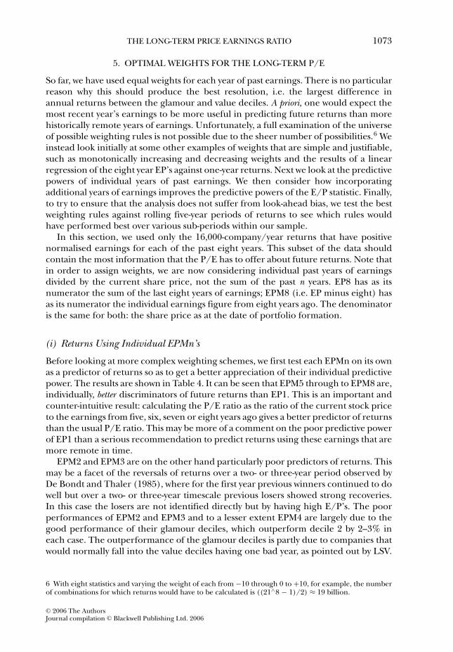
Before looking at more complex weighting schemes, we first test each EPMn on its ownas a predictor of returns so as to get a better appreciation of their individual predictivepower. The results are shown in Table 4. It can be seen that EPM5 through to EPM8 are,individually, better discriminators of future returns than EP1. This is an important andcounter-intuitive result: calculating the P/E ratio as the ratio of the current stock priceto the earnings from five, six, seven or eight years ago gives a better predictor of returnsthan the usual P/E ratio. This may be more of a comment on the poor predictive powerof EP1 than a serious recommendation to predict returns using these earnings that aremore remote in time.

EPM2 and EPM3 are on the other hand particularly poor predictors of returns. Thismay be a facet of the reversals of returns over a two- or three-year period observed byDe Bondt and Thaler (1985), where for the first year previous winners continued to dowell but over a two- or three-year timescale previous losers showed strong recoveries.In this case the losers are not identified directly but by having high E/P’s. The poorperformances of EPM2 and EPM3 and to a lesser extent EPM4 are largely due to thegood performance of their glamour deciles, which outperform decile 2 by 2–3% ineach case. The outperformance of the glamour deciles is partly due to companies thatwould normally fall into the value deciles having one bad year, as pointed out by LSV.

6 With eight statistics and varying the weight of each from −10 through 0 to +10, for example, the numberof combinations for which returns would have to be calculated is ((21∧8 − 1)/2) ≈ 19 billion.



Table 4Average One-Year Returns After Assigning Companies to Decile Portfolios Using

Individual Past Years of Earnings EP1 Through to EPM8

EP1 EPM2 EPM3 EPM4 EPM5 EPM6 EPM7 EPM8Alone % Alone % Alone % Alone % Alone % Alone % Alone % Alone %

High P/E 18.03 20.66 19.72 18.47 16.14 16.46 16.39 16.24Decile 2 19.18 18.06 16.88 16.61 16.52 17.10 16.64 17.05Decile 3 18.05 19.11 18.78 17.41 16.15 17.66 18.01 16.50Decile 4 15.26 19.31 18.87 18.23 18.64 16.30 16.05 18.32Decile 5 19.56 16.91 18.22 18.23 19.35 18.68 20.65 18.00Decile 6 18.01 19.19 18.34 19.19 19.55 20.99 19.80 20.44Decile 7 19.72 19.65 19.96 20.82 20.45 21.13 18.73 19.94Decile 8 20.28 20.51 18.78 21.67 22.80 20.60 21.39 22.23Decile 9 24.11 21.31 23.93 21.50 21.87 21.70 23.22 22.43Low P/E 26.34 23.86 25.11 26.46 27.12 27.97 27.69 27.40D10 – D1 8.31 3.20 5.38 7.99 10.98 11.51 11.30 11.15

Note:The EP1 returns are repeated from Table 1 Panel B. All UK stocks with eight years of positiveearnings are used, 1975–2003.

For example, there were 48 company/year returns that fell into EPM3’s glamour decilebecause they showed particularly weak earnings three years ago, when on the basis ofan equally weighted average of the other seven years of earnings they should have beenplaced in the value decile. These companies showed average one-year returns of 41.6%.

(ii) Returns from Simple Weighting Schemes

The simplest possible weighting scheme is equal weights, returns for which we alreadyreported in Section 3. In addition, we tried linearly increasing weights, so that the mostrecent year of earnings has the greatest weight, and weights that increase according toan inverse square law, so that the most recent year has an even heavier weight. So asto show the relative value of more recent years of earnings, we also calculated returnsfor mirror-image weighting schemes that decrease linearly or according to the inversesquare law. According to our a priori expectations these should perform poorly, sincewe expect the most recent earnings to have the most predictive power. We report decilereturns for these weighting schemes in columns 1 to 5 of Table 5.

The 11.62% value premium seen in Table 5 for equal weights is the standardagainst which all other results should be measured. If other weighting regimes cannotoutperform this simple system by a worthwhile margin then the constant weightsshould be retained. Of the other four weighting systems, the reverse weights are bestwith straight-line reverse weighting giving the highest value premium of 12.17%. Boththe reverse weighting systems provide resolutions considerably superior to those ofthe ‘forwards’ weighting systems. This is contrary to the a priori expectation thatmore recent earnings would be more relevant to predicting returns than earningsfurther back in time. The explanation can be found in the resolutions achieved bythe individual EPMns reported above: the particularly poor predictive power of EPM2and EPM3 means that any scheme that weights these two heavily will perform poorly.




Different EP1-EPM8 Weighting Rules

1 2 3 4 5 6

Increasing Weights Decreasing WeightsLinear Regression

Equal Weights Linear Inverse Square Linear Inverse Square Weights

Weights AssignedEP1 1 8 1 1 1/64 0.8442EPM2 1 7 1

4 2 1/49 −0.1794EPM3 1 6 1/9 3 1/36 −0.3327EPM4 1 5 1/16 4 1/25 0.4347EPM5 1 4 1/25 5 1/16 0.1897EPM6 1 3 1/36 6 1/9 0.0223EPM7 1 2 1/49 7 1

4 0.1235EPM8 1 1 1/64 8 1 0.0499

One-Year ReturnsHigh P/E 16.26% 16.89% 17.84% 15.81% 15.19% 16.68%Decile 2 16.71% 16.30% 16.44% 16.05% 16.79% 14.83%Decile 3 16.43% 18.10% 18.03% 16.95% 16.52% 17.40%Decile 4 18.42% 17.24% 17.48% 18.35% 19.05% 17.60%Decile 5 19.54% 18.93% 17.96% 19.14% 19.00% 19.77%Decile 6 19.81% 19.66% 20.03% 20.69% 19.42% 18.28%Decile 7 19.39% 20.11% 20.76% 19.92% 20.80% 20.36%Decile 8 21.11% 20.79% 21.50% 20.27% 21.00% 22.33%Decile 9 23.05% 23.83% 20.77% 23.48% 23.84% 22.89%Low P/E 27.87% 26.68% 27.75% 27.98% 27.01% 28.45%D10 – D1 11.62% 9.79% 9.91% 12.17% 11.82% 11.77%

Notes:The data are all UK stocks with eight years of positive earnings, 1975-2003. Read each column as aseparate calculation of returns over the 29 years, that first shows the weights applied, then the decileportfolio returns resulting from assigning companies to deciles using a P/E constructed from those weights.The equally-weighted returns are repeated from Table 1 Panel B.

The even heavier weight given to EP1 under any ‘forward’ weighting is not enough tocounterbalance this weakness.

(iii) Predicting Returns From the EPMn with a Linear Regression

In order to examine whether a linear regression yields better weights of the historicalearnings, we ran a regression against the 16,000 company/year returns that havepositive earnings for each of the last eight years. We expected it to give us an optimalweighting system that would outperform any of the resolutions seen so far. The model is:

Rtn01i = β0 + β1EP1i + β2EPM2i + β3EPM3i + β4EPM4i

+ β5EPM5i + β6EPM6i + β7EPM7i + β8EPM8i + ui (4)

where Rtn01i is the one-year holding period return for company-year i, EP1 is the EPcalculated on the basis of the previous year’s earnings, EPMji is the EP calculated fromthe earnings two through to eight years ago and ui is a disturbance term.




EP1 Plus (EPM2 through to EPM8)

EP1 + EP1 + EP1 + EP1 + EP1 + EP1 + EP1 +EPM2 EPM3 EPM4 EPM5 EPM6 EPM7 EPM8

Weights AssignedEP1 1 1 1 1 1 1 1EPM2 1 0 0 0 0 0 0EPM3 0 1 0 0 0 0 0EPM4 0 0 1 0 0 0 0EPM5 0 0 0 1 0 0 0EPM6 0 0 0 0 1 0 0EPM7 0 0 0 0 0 1 0EPM8 0 0 0 0 0 0 1

One-Year ReturnsHigh P/E 18.52% 18.32% 17.32% 17.11% 16.76% 16.71% 16.21%Decile 2 17.42% 16.73% 16.37% 15.68% 16.86% 16.82% 16.15%Decile 3 18.60% 17.67% 16.79% 15.69% 15.68% 15.71% 17.27%Decile 4 17.25% 17.93% 17.68% 18.49% 17.47% 17.58% 16.55%Decile 5 19.16% 18.18% 17.49% 18.59% 18.74% 18.73% 20.03%Decile 6 19.51% 19.36% 20.36% 19.98% 19.49% 19.44% 18.13%Decile 7 19.78% 20.38% 21.41% 20.78% 21.12% 19.18% 20.06%Decile 8 21.33% 21.92% 22.53% 21.30% 20.81% 23.90% 23.34%Decile 9 21.07% 21.54% 21.69% 22.49% 23.43% 22.69% 21.92%Low P/E 25.93% 26.51% 26.95% 28.46% 28.25% 27.82% 28.95%D10 – D1 7.41% 8.19% 9.63% 11.36% 11.49% 11.12% 12.73%

Note:All UK stocks with eight years of positive earnings are used, 1975-2003.

The coefficients from the regression are shown in the top part of column 6 in Table 5.EP1, EPM3 and EPM4 are significant at the 0.1% level, EPM2 is significant at the 5%level, but EPM5-EPM8 are not significant. EP1, in accordance with our expectations,has twice the weight of EPM2-EPM4. Earnings more than four years old have small butpositive parameter values. However, although EPM2 and EPM3 are positive indicatorsof returns when taken alone, when combined with the information available in theother EPMn they have significant negative coefficients, entirely contrary to what onewould expect.

Looking at the last row of Table 5, the resolution of 11.77% achieved by the linearregression is only fractionally better than the 11.62% achieved by using equal weights.It is poorer than the resolution of 12.17% for reverse linear weights. This approachdoes not therefore give optimal weights even when using all of the data in a singleregression. This result is slightly surprising for it suggests that the equal weighting ishard to improve upon even with perfect foresight concerning the optimal weights touse. This may be due to some degree of collinearity between adjacent EPM figures. Itmay also be that the regression is a linear one but the portfolio approach to evaluatingthe power of the price-earnings ratio is inherently non-linear.7

7 We thank an anonymous referee for proposing this explanation.



Table 7Correlations Between the Eight Individual Past Years of Earnings

EPM7 EPM6 EPM5 EPM4 EPM3 EPM2 EP1

EPM8 0.8267 0.6984 0.6320 0.5415 0.4762 0.3779 0.2765EPM7 0.8180 0.7258 0.6095 0.5324 0.4263 0.2959EPM6 0.8023 0.6553 0.5493 0.4209 0.3012EPM5 0.8180 0.6602 0.5137 0.3431EPM4 0.7954 0.6100 0.3891EPM3 0.7317 0.4702EPM2 0.6136

Note:All UK stocks with eight years of positive earnings are used, 1975-2003.

(iv) Returns Using Two EPMns

Considering the failure of the linear regression to yield a superior resolution, doescombining two or more of the EPMn yield better results than the individual EPMns? EP1is the standard figure for the P/E ratio. As such it should presumably be included in anyweighted average of EPMns. Table 6 shows the resolutions available from combiningEP1 with each of the other EPMn figures. We make no attempt to attach fractionalweights; the figures for the earnings last year and for the earnings n years ago aresimply added together, then divided by the current share price. The resolution offeredby the best weighting scheme found so far, the reverse linear weights, is bettered byusing EP1 plus EPM8. Also of note is that EP1 plus EPM2, and EP1 plus EPM3, givea poorer resolution than EP1 alone. EPM2 and EPM3 when included with EP1 havetaken away value from the combined statistic, even though when used alone EPM2 andEPM3 give a small but nevertheless positive resolution figure.

Some explanation of the observed resolutions of the different EPMn pairs is offeredby looking at their correlations in Table 7. Correlations between adjacent years of EPMnfigures are particularly high, in the region 0.7 to 0.8. It is therefore not surprising thatif an EP statistic is created by adding EPMn figures from adjacent years it adds littleresolution to the underlying EPMn values. The low 0.28 correlation between EP1 andEPM8, presumably due to their remoteness in time to each other, may also explain thehigh resolution found by adding the two values together.8

(v) Data Mining?

The linear regression may fairly be said to suffer from look-ahead bias, in that it takesweights derived from a regression on our whole dataset then tests its efficacy over thesame 1975 to 2003 period. Even using this look-ahead bias it is unable to beat someof the simpler weighting schemes. Although these simpler schemes do not suffer fromlook-ahead bias, they have also so far only been tested against the entire 1975–2003period.

8 We also examined triple combinations of the EPMn figures. Adding in a third EPMn figure to EP1 andEPM8 reduced the one-year holding period resolution of the combined statistic in every case except usingEPM4. Here, the average returns were increased by 0.4%, and Occam’s Razor therefore suggests that thesimple (EP1 + EPM8) statistic be adhered to, rather than adding in a third EPMn.



Table 8Summary Statistics From Calculating Individual Year Resolutions for Various

Weighting Rules, 1975–2003

Linear Descending Linear Ascending EP1Equal Linear Weights, Weights, EP1 +EPM4

Weights Regression EPM8 Largest EP1 Largest +EPM8 +EPM8

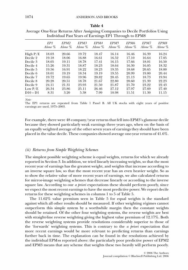
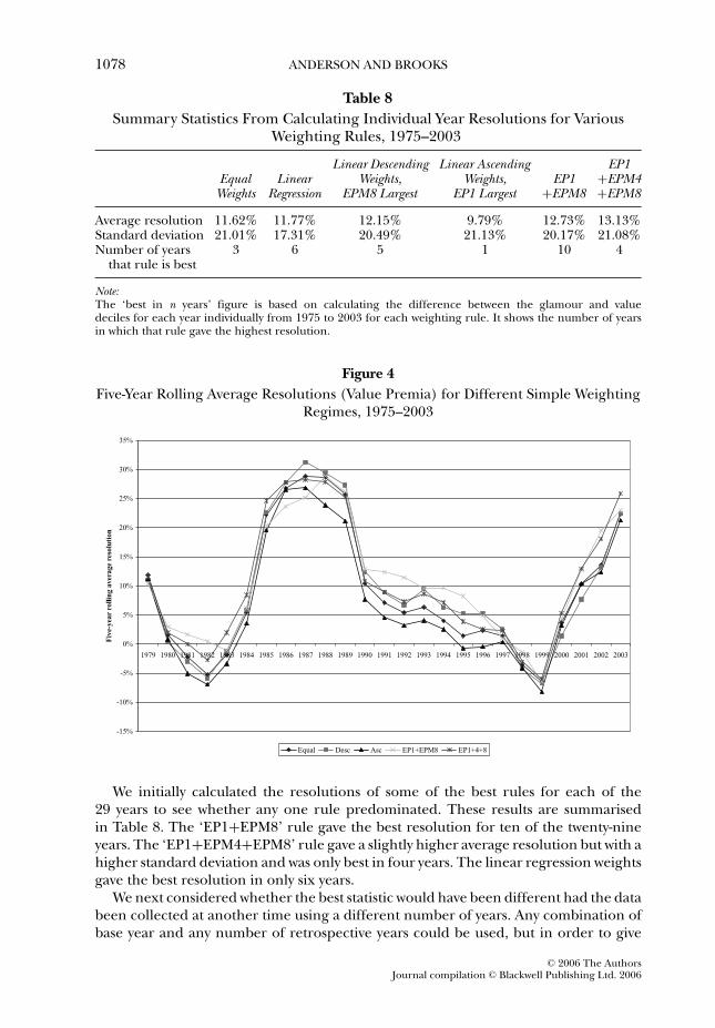
Average resolution 11.62% 11.77% 12.15% 9.79% 12.73% 13.13%Standard deviation 21.01% 17.31% 20.49% 21.13% 20.17% 21.08%Number of years 3 6 5 1 10 4

that rule is best

Note:The ‘best in n years’ figure is based on calculating the difference between the glamour and valuedeciles for each year individually from 1975 to 2003 for each weighting rule. It shows the number of yearsin which that rule gave the highest resolution.

Figure 4Five-Year Rolling Average Resolutions (Value Premia) for Different Simple Weighting

Regimes, 1975–2003

-15%

-10%

-5%

0%

5%

10%

15%

20%

25%

30%

35%

1979 1980 1981 1982 1983 1984 1985 1986 1987 1988 1989 1990 1991 1992 1993 1994 1995 1996 1997 1998 1999 2000 2001 2002 2003

Fiv

e-ye

ar r

ollin

g av

erag

e re

solu

tion

Equal Desc Asc EP1+EPM8 EP1+4+8

We initially calculated the resolutions of some of the best rules for each of the29 years to see whether any one rule predominated. These results are summarisedin Table 8. The ‘EP1+EPM8’ rule gave the best resolution for ten of the twenty-nineyears. The ‘EP1+EPM4+EPM8’ rule gave a slightly higher average resolution but with ahigher standard deviation and was only best in four years. The linear regression weightsgave the best resolution in only six years.

We next considered whether the best statistic would have been different had the databeen collected at another time using a different number of years. Any combination ofbase year and any number of retrospective years could be used, but in order to give



some comparability to the results, we selected a rolling five-year period. This yieldsa sufficiently large number of company/year returns for each five-year period (atleast 2,300). Figure 4 plots the rolling (overlapping) five-year average resolution foreach of the simple weighting schemes in Table 8, excluding the linear regression. Theresolution in Figure 4 is then the average of the five individual year resolutions. Themost visible conclusion is that the resolutions follow each other quite closely whicheverweighting system is chosen. 1982 and 1999 were low points for any value-glamourarbitrage strategy. Indeed in 1998 and 1999 every weighting system had providednegative returns to the arbitrageur over the previous five years. However, since thenthere has been a resounding resurgence similar to that seen in 1982-1985. By 2003,average resolutions over the previous five years exceeded 20% per year. Over the wholeperiod, no one weighting system predominates, but adding the previous year’s earningsto the earnings eight years ago is often best. Ascending weights, that might a priori havebeen thought to be the most reasonable as they assign the most weight to the mostrecent E/P, are often the worst amongst the weighting rules charted. The rolling five-year returns at least give some confidence that much the same conclusion would havebeen reached had our investigation been carried out at any time over the past 29 years.

6. THE EFFECT OF THE BID-ASK SPREAD, RISK AND LIQUIDITY

It is often suggested that the effectiveness of value-based investment strategies will bemuch reduced once transaction costs are taken into account. Although commissioncharges applicable to the deciles will be similar, since they consist of similar numbersof shares and are rebalanced over the same periods, the effect of the bid-ask spread willbe different between the deciles.9 As shown below, low P/E firms tend to be smallercompanies that have larger spreads. How much does allowing for the effect of lossesfrom the bid-ask spread reduce the difference in returns between the deciles? A relatedpossible problem is that smaller companies are likely to have poorer liquidity. Will thetrades of a typical investor cause liquidity problems for the shares of small companiesthat are concentrated in the value decile? To determine the impact of transactionscosts on strategy returns, we divided companies into 20 categories based on marketcapitalisation, calculated the spreads as they affect one-year returns and averaged themover each market value category. The results are shown in Table 9 and Figure 5. Thespread costs shown in Figure 5 range quite smoothly from 8.2% for the smallest 5% ofcompanies, to only 0.95% for the largest 5%.

The changes to compound annual returns after allowing for transaction costs usingannual rebalancing are shown in Table 10. Returns for each decile are shown, with andwithout the bid-ask spread taken into account in one-year returns. Also shown are theaverage market value categories for each decile. The value premium is reduced by 2.6%and the returns on the value decile reduce by 4.18% from 28.95% to 24.77%. The factthat smaller companies tend to have lower P/E’s and therefore tend to appear in thevalue decile can be seen by looking at the ‘MV Category’ column. The value decile hasan average MV category of 6.01, which is equivalent to an average market capitalisationof £44m in 2003. This rises to MV category 11.65 ( £190m) for the glamour decile.

9 Investors must also pay a 0.5% UK tax known as stamp duty on all share purchases. This will reduce returnsby up to 0.5% per annum, depending on stock turnover within each decile. Since it will affect the decilesroughly equally, we do not incorporate it into our calculations.



Table 9Average Bid-Ask Spread Costs on One-Year Returns, Grouping by Market Value

Category, 1987–2003

MV Category 1 2 3 4 5 6 7 8 9 10

Total spread 8.20% 6.92% 5.72% 4.62% 4.42% 4.32% 3.59% 3.42% 3.04% 2.65%

MV Category 11 12 13 14 15 16 17 18 19 20

Total spread 2.42% 2.37% 2.24% 1.93% 1.72% 1.60% 1.58% 1.53% 1.32% 0.95%

Note:Bid and ask prices are only available from Datastream starting in 1987.

Figure 5Average Cost of the Bid-Ask Spread to One-Year Returns Grouped by Market Value

Category, 1987–2003

0%

1%

2%

3%

4%

5%

6%

7%

8%

9%

1 2 3 4 5 6 7 8 9 10 11 12 13 14 15 16 17 18 19 20

MV Category

Bid/OfferSpread

Overall, the reduction in returns caused by the bid-ask spread is serious but notcatastrophic to a P/E-based strategy. If shares were sorted into deciles purely by size, wewould expect spreads to reduce the value premium by the difference in bid-ask chargesfor MV categories 1 and 2 compared to MV categories 19 and 20. From Table 9, thisis 6.43%. In fact it is reduced by 2.6%, or only one-fifth of the value premium. Thisis partly because the glamour and value deciles are not made up exclusively of largeand small shares respectively, and partly because not all shares are sold and re-boughtannually. If shares ‘roll over’ from one year to the next because they appear in the samedecile this reduces the spread costs. It is clear that the bid-ask spread can only accountfor a small proportion of the difference in returns between the value and glamourdeciles.



Table 10Compound Annual Returns, Average Market Value Category (1–20) and AverageMarket Betas for ‘EP1+EPM8’ With and Without the Effect of the Bid-Ask Spread

on Returns

Return % Return Net of Spread % MV Category Beta

High P/E 16.21 14.64 11.65 1.0232Decile 2 16.15 13.93 12.64 0.9594Decile 3 17.27 14.78 12.72 0.9905Decile 4 16.55 13.99 12.16 0.9589Decile 5 20.03 17.26 11.69 0.9440Decile 6 18.13 15.12 11.03 0.9266Decile 7 20.06 16.67 10.04 0.9577Decile 8 23.34 19.59 9.20 0.9123Decile 9 21.92 18.08 7.91 0.9277Low P/E 28.95 24.77 6.01 0.9998D10 - D1 12.73 10.13 - -

Table 11Returns for Extreme Deciles of Portfolios Sorted by EP1, EP8, Book Value-to-Price

and Market Capitalisation, Over Holding Periods of 1 to 8 Years

Sort 1 Year 2 Years 3 Years 4 Years 5 Years 6 Years 7 Years 8 Yearsby Portfolio % % % % % % % %

EP1 Decile 1 13.65 16.28 13.85 13.91 13.00 13.17 13.09 13.28Decile 10 20.85 22.81 21.83 20.16 19.01 17.53 16.93 16.64D10 - D1 7.21 6.52 7.98 6.25 6.01 4.36 3.84 3.36

EP8 Decile 1 11.65 14.13 11.11 9.93 9.82 10.00 9.90 10.51Decile 10 23.19 25.34 23.72 21.75 20.79 18.62 18.03 17.76D10 - D1 11.54 11.20 12.61 11.82 10.97 8.62 8.13 7.25

Book value- Decile 1 14.47 16.50 14.00 12.93 12.67 12.74 12.46 12.53to-price Decile 10 22.82 25.09 23.45 22.23 20.98 18.90 17.98 17.47

D10 - D1 8.35 8.59 9.45 9.30 8.31 6.16 5.52 4.94

Market capital- Decile 1 10.91 12.14 11.87 11.89 12.12 12.45 12.53 12.58isation Decile 10 22.69 25.30 24.00 21.84 19.81 17.74 16.74 16.41

D10 - D1 11.78 13.16 12.12 9.95 7.69 5.29 4.21 3.83

The final column of Table 10 shows the CAPM betas for each decile portfolio. Thesebetas are very similar across the deciles, with slightly lower betas for the value decilethan the growth decile. We thus find that, in common with previous studies, the valuepremium cannot be rationalised by risk in the sense of the CAPM.

In Table 11 we consider whether book value-to-price and firm size would be equallyuseful discriminators of company stock performance. The table presents the extremedecile returns for stocks separately sorted using EP1, EP8, book value-to-price andmarket capitalisation for investment horizons of 1 to 8 years. We recalculate theEP1 and EP8 results since the analysis is now conducted on a smaller sample of8,300 company-years for which book values are available. Incorporating eight yearsof earnings information into the EP statistic rather than just one year again results



Table 12Median Number of Days of Turnover Represented by Each Trade, for a PrivateInvestor with £50,000 in 2003 and for a Hedge Fund with £20m (EP1 and EP8

are used to assign companies to deciles)

EP1 EP8

Days of Days of Days of Days ofTurnover for Turnover for Turnover for Turnover for

Decile Private Investor Hedge Fund Private Investor Hedge Fund

High P/E 0.0023 0.93 0.0005 0.202 0.0009 0.38 0.0005 0.183 0.0013 0.51 0.0004 0.174 0.0008 0.30 0.0004 0.155 0.0008 0.32 0.0007 0.266 0.0011 0.42 0.0008 0.317 0.0015 0.62 0.0008 0.338 0.0021 0.84 0.0022 0.899 0.0035 1.41 0.0058 2.30Low P/E 0.0084 3.37 0.0114 4.54

in a stronger value premium for this sub-sample of companies. There is also a clearsize premium, with the smallest 10% of companies yielding stock returns around 12%higher than those of the largest 10% of companies for holding periods of up to 3 years.For these shorter investment horizons, the size premium is similar in magnitude to theEP8 value premium. However, the size premium would be the most seriously affectedby the differential bid-ask spreads between larger and smaller companies. Book value-to-price, the value measure favoured by Fama and French, is a stronger discriminatorof returns than the traditional P/E ratio, but weaker than the modified P/E ratio thatemploys a longer history of earnings.

We also checked whether the limited liquidity of some shares would have causeddifficulties for investors. Datastream has daily turnover figures for most companiesstarting in 1987. We assumed a representative private investor with £50,000 to invest in2003 and a hedge fund with £20m. We deflated these portfolio values going backwardsin time by the average market return. For example, in 2002–2003 the average returnwas unusually negative at −15.22%, so our private portfolio value for 2002 was largerat £58,975. Table 12 shows the median number of days of turnover represented by thetrades of these two sample investors, using EP1 and EP8 to assign companies to deciles.For the private investor, the trades conducted usually represent only a small proportionof a day’s turnover in the shares, so he will rarely face liquidity problems. Investing inthe glamour decile will also present no liquidity problems for the hedge fund eventhough its trades are 400 times as large, because the glamour decile consists mostly oflarge companies. Where problems are likely to occur is the value decile because smallcompanies are concentrated here. For this decile the median trade represents 3.37 daysof turnover using EP1, so even a small institutional investor would often have to spreadthe required trades over several days to avoid moving the market adversely. However,since the strategy is not particularly time-dependent, this is not likely to be a majorissue. The liquidity problem is slightly worse using EP8, with a median trade size of4.54 days’ turnover.



Table 13Portfolio Values and Percentage Returns for Glamour and Value Deciles Using

EP1 and (EP1 + EPM8) to Assign Companies to Deciles, 1975-2003

EP1+EPM8 EP1 (traditional EP)

Value Decile Glamour Decile Value Decile Glamour Decile

Value in 1975 £1,000 £1,000 £1,000 £1,000Value in 2004 £952,028 £44,539 £548,274 £70,350Compound Return 26.68% 13.99% 24.29% 15.80%

Figure 6Portfolio Values for the Value and Glamour Deciles Using EP1 and (EP1 + EPM8) to

Sort Companies into Deciles, Annual Rebalancing, 1975–2003

£1,000

£10,000

£100,000

£1,000,000

1975

1976

1977

1978

1979

1980

1981

1982

1983

1984

1985

1986

1987

1988

1989

1990

1991

1992

1993

1994

1995

1996

1997

1998

1999

2000

2001

2002

2003

2004

Por

tfol

io v

alu

e

EP1 Value EP1 Glamour EP1+EPM8 Value EP1+EPM8 Glamour

7. PORTFOLIO ILLUSTRATION

The following example shows the impact on returns of optimising the weights of the pasteight years of earnings, compared to the original P/E. We calculated the performancesof the value and glamour deciles identified using the (EP1+EPM8) statistic andcompared them to the returns for the deciles calculated using the traditional P/E ratioEP1. All portfolios use annual rebalancing. The final values and compound returns areshown in Table 13 and the values of the four portfolios are shown graphically in Figure 6.The new value decile as calculated using (EP1+EPM8) outperforms the value decilefrom EP1 and the new glamour decile underperforms, so that the previous decilesare bracketed by the new deciles. Our use of a logarithmic scale in Figure 6 does notgive a visual impression of dramatic outperformance or underperformance. However,over 29 years the compounding effect results in a new value decile worth almost twice



as much as the old value decile, and a new glamour decile worth two-thirds the oldglamour decile. The value premium is thus considerably enhanced.

8. CONCLUSION

Graham and Dodd (1934) suggested that multiple years of earnings should be usedto assess the long-term value of a company. Although using multiple years of earningsseems a very natural way of measuring fundamental value, we are not aware of any pre-vious investigations into whether several years of earnings are more useful in predictingreturns than one year. Our results suggest that a P/E calculated from multiple years ofearnings is a better predictor of returns than the traditional one-year P/E. An eight-year average is twice as effective. However, the difference between returns from theglamour and value deciles does not increase linearly as more past years are added intothe calculation. Earnings from two or three years ago are particularly poor predictors.

We examined several plausible weighting rules for the past years of earnings, usingthe subset of companies with a full eight years of positive normalised earnings. Theindividual earnings figures from five, six, seven or eight years ago, divided by the currentshare price, are better predictors of returns than the traditional P/E. This is testamentto the limitations of the usual P/E ratio for predicting returns. We found that a sortstatistic based on (EP1+EPM8) gave the best resolution between the value and glamourdeciles, ignoring the other six earnings figures, as these two earnings figures have arelatively low correlation. This increased the value premium from 5.98% to 12.73%.

Finally, we attempted to deal with three possible criticisms. We used rolling five-year data windows to show that the (EP1+EPM8) statistic or something very similarwould have been the best statistic over most of the last 29 years, whenever a similarinvestigation had been performed and whatever retrospective period of data it used.We also showed that although the bid-ask spread has a differential effect on the returnsof the value and glamour deciles, it could only account for a small proportion of thevalue premium. We demonstrated that liquidity is only likely to present problems foran institutional investor buying the small company shares concentrated in the valuedecile. Even so, if the purchases are spread over several days then the price impacts arelikely to be modest.

The results presented in this paper suggest several potential avenues for furtherresearch. An obvious follow-on would be to determine whether these findings holdtrue in the much larger US market. We do not doubt that multiple years of earningswill be more useful than one, but it will be interesting to find out whether US earningsfrom two and three years ago should be negatively weighted and whether the earningsfrom five to eight years ago are better at predicting returns than the usual P/E. Inthe US case, transactions costs and illiquidity are likely to be even less of an issue.Finally, our results suggest the presence of a large and persistent value premium thatwould be hard to rationalise using standard asset pricing models. It is thus possiblethat behavioural explanations hold the key. Future research may examine competingpsychological models in detail.

REFERENCES

Aggarwal, R., R.P. Rao and T. Hiraki (1990), ‘Regularities in Tokyo Stock ExchangeSecurity Returns: P/E, Size, and Seasonal Influences’, Journal of Financial Research,Vol. 13, pp. 249–63.



Ball, R. (1978), ‘Anomalies in Relationships Between Securities’ Yields and Yield-Surrogates’,Journal of Financial Economics, Vol. 6, pp. 103–26.

——— (1992), ‘The Earnings-Price Anomaly’, Journal of Accounting and Economics, Vol. 15, Nos.2&3, pp. 319–45.

Banz, R.W. and W.J. Breen (1986), ‘Sample-Dependent Results Using Accounting and MarketData: Some Evidence’, Journal of Finance, Vol. 41, No. 4, pp. 779–93.

Basu, S. (1975), ‘The Information Content of Price-Earnings Ratios’, Financial Management,Vol. 4, No. 2, pp. 53–64.

——— (1977), ‘The Investment Performance of Common Stocks in Relation to Their Price-Earnings Ratios’, Journal of Finance, Vol. 32, No. 3, pp. 663–82.

Bird, R. and J. Whitaker (2003), ‘The Performance of Value and Momentum InvestmentPortfolios: Recent Experience in the Major European Markets, Journal of Asset Management,Vol. 4, No. 4, pp. 221–46.

Booth, G.G., T. Martikainen, J. Perttunen and P. Yli-Olli (1994), ‘On the Functional Form ofEarnings and Stock Prices: International Evidence and Implications for the P/E Anomaly’,Journal of Business Finance & Accounting , Vol. 21, No. 3, pp. 395–408.

Brouwer, I., J. van der Put and C. Veld (1997), ‘Contrarian Investment Strategies in a EuropeanContext’, Journal of Business Finance & Accounting , Vol. 24, Nos. 9&10, pp. 1353–66.

Cai, J. (1997), ‘Glamour and Value Strategies on the Tokyo Stock Exchange’, Journal of BusinessFinance & Accounting , Vol. 24, Nos. 9 & 10, pp. 1291–310.

Campbell, J.Y. and R.J. Shiller (1988), ‘Stock Prices, Earnings, and Expected Dividends’, Journalof Finance, Vol. 43, No. 3, pp. 661–76.

Chan, L.C.K., Y. Hamao and J. Lakonishok (1991), ‘Fundamentals and Stock Returns in Japan’,Journal of Finance, Vol. 46, No. 5, pp. 1739–64.

Chin, J.Y.F., A.K. Prevost and A.A. Gottesman (2002), ‘Contrarian Investing in a SmallCapitalization Market: Evidence from New Zealand’, Financial Review, Vol. 37, No. 3, pp.421–46.

Chou, S.-R. and K.H. Johnson (1990), ‘An Empirical Analysis of Stock Market Anomalies:Evidence from the Republic of China in Taiwan’, in S.G. Rhee and R.P. Chang (eds.),Pacific-Basin Capital Markets Research (North-Holland: Elsevier Science Publishers).

De Bondt, W.F.M. and R. Thaler (1985), ‘Does the Stock Market Overreact?’ Journal of Finance,Vol. 40, No. 3, pp. 793–805.

Doeswijk, R.Q. (1997), ‘Contrarian Investment in the Dutch Stock Market’, De Economist,Vol. 145, No. 4, pp. 573–98.

Dreman, D.N. (1998), Contrarian Investment Strategies: The Next Generation (New York: Simonand Schuster).

Fama, E.F. and K.R. French (1992), ‘The Cross-Section of Expected Stock Returns’, Journal ofFinance, Vol. 47, No. 2, pp. 427–65.

——— ——— (1993), ‘Common Risk Factors in the Returns on Stocks and Bonds’, Journal ofFinancial Economics, Vol. 33, No. 1, pp. 3–56.

——— ——— (1996), ‘Multifactor Explanations of Asset Pricing Anomalies’, Journal of Finance,Vol. 51, No. 1, pp. 55–84.

——— ——— (1998), ‘Value versus Growth: The International Evidence’, Journal of Finance,Vol. 53, No. 6, pp. 1975–99.

Fuller, R.J., L.C. Huberts and M.J. Levinson (1993), ‘Returns to E/P Strategies, HiggeldyPiggeldy Growth, Analysts’ Forecast Errors, and Omitted Risk Factors’, Journal of PortfolioManagement (Winter), pp. 13–24.

Graham, B. and D. Dodd (1934), Security Analysis (New York: McGraw-Hill).Gregory, A., R.D.F. Harris and M. Michou (2001), ‘An Analysis of Contrarian Investment

Strategies in the UK’, Journal of Business Finance & Accounting , Vol. 28, Nos. 9 & 10,pp. 1193–228.

Jaffe, J., D.B. Keim and R. Westerfield (1989), ‘Earnings Yields, Market Values, and StockReturns’, Journal of Finance, Vol. 44, No. 1, pp. 135–48.

Jegadeesh, N. and S. Titman (1993), ‘Returns to Buying Winners and Selling Losers:Implications for Stock Market Efficiency’, Journal of Finance, Vol. 48, No. 1, pp. 65–91.

Lakonishok, J., A. Schleifer and R. Vishny (1994), ‘Contrarian Investment, Extrapolation, andRisk’, Journal of Finance, Vol. 49, No. 5, pp. 1541–78.



Levis, M. (1989), ‘Stock Market Anomalies’, Journal of Banking and Finance, Vol. 13, pp. 675–96.Levis, M. and M. Liodakis (2001), ‘Contrarian Strategies and Investor Expectations: The U.K.

Evidence’, Financial Analysts Journal , Vol. 57, No. 5, pp. 43–46.Nicholson, S.F. (1960), ‘Price-Earnings Ratios’, Financial Analysts Journal , Vol. 16, No. 4,

pp. 43–45.——— (1968), ‘Price-Earnings Ratios in Relation to Investment Results’, Financial Analysts

Journal , Vol. 24, No. 1, pp. 105–09.Park, Y.S. and J.-J. Lee (2003), ‘An Empirical Study on the Relevance of Applying Relative

Valuation Models to Investment Strategies in the Japanese Stock Market’, Japan and theWorld Economy, Vol. 15, pp. 331–39.

Shiller, R.J. (2000), Irrational Exuberance (Princeton: Princeton University Press).


the long-term price-earnings ratio - ka536/long-term pe.pdf · the long-term price earnings ratio...

Documents