©the mcgraw-hill companies, inc. 2008mcgraw-hill/irwin lesson 12
TRANSCRIPT

©The McGraw-Hill Companies, Inc. 2008McGraw-Hill/Irwin
Time Series and Forecasting
Lesson 12

Define the components of a time series Compute moving average Determine a linear trend equation Compute a trend equation for a nonlinear
trend Use a trend equation to forecast future time
periods and to develop seasonally adjusted forecasts
Determine and interpret a set of seasonal indexes
Deseasonalize data using a seasonal index Test for autocorrelation
2
Goals

What is a time series?◦a collection of data recorded over a period of time (weekly, monthly, quarterly)
◦an analysis of history, it can be used by management to make current decisions and plans based on long-term forecasting
◦Usually assumes past pattern to continue into the future
3
Time Series

Secular Trend – the smooth long term direction of a time series
Cyclical Variation – the rise and fall of a time series over periods longer than one year
Seasonal Variation – Patterns of change in a time series within a year which tends to repeat each year
Irregular Variation – classified into:Episodic – unpredictable but identifiableResidual – also called chance fluctuation and unidentifiable
4
Components of a Time Series

5
Cyclical Variation – Sample Chart
6
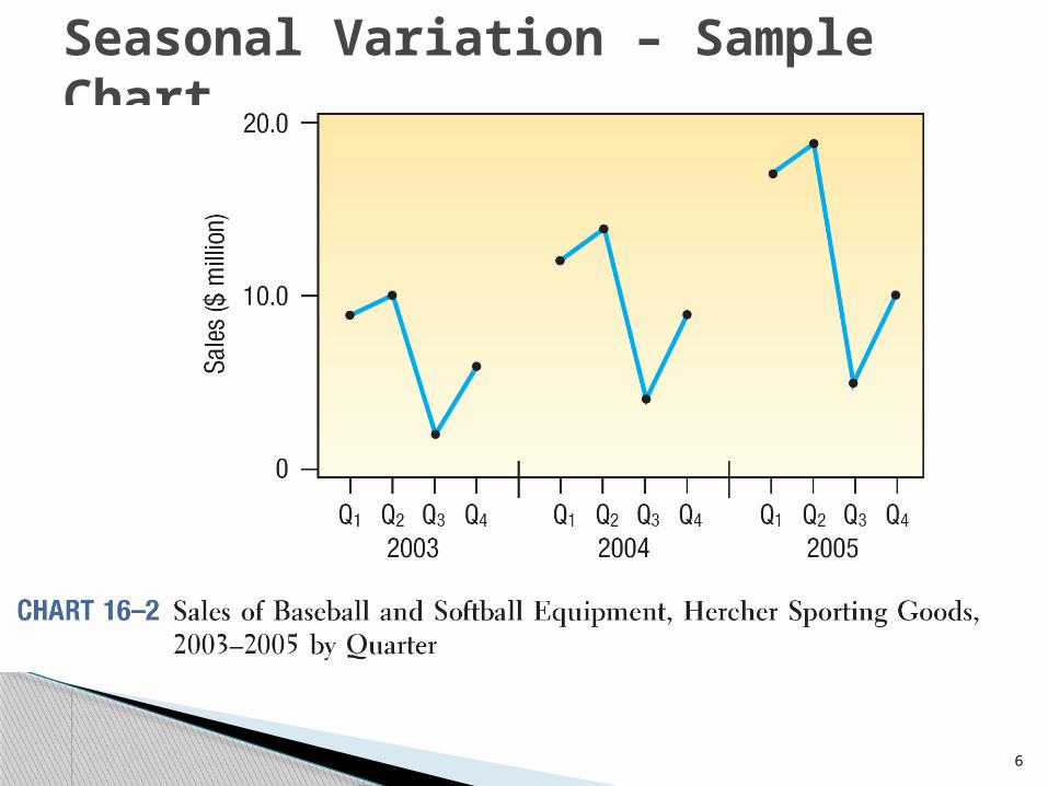
Seasonal Variation – Sample Chart

7
Secular Trend – Home Depot Example

Components of a Time Series
8
Sales
Time
Seasonality
Trend Line
Cycle
Irregular component

Useful in smoothing time series to see its trend
Basic method used in measuring seasonal fluctuation
Applicable when time series follows fairly linear trend that have definite rhythmic pattern
9
The Moving Average Method

Moving Average Method - Example
Time Response Moving Total Moving2002 4 NA NA2003 6 4 + 6 + 5 = 15 15/3 = 5.02004 5 6 + 5 + 3 = 14 14/3 = 4.72005 3 5 + 3 + 7 = 15 15/3 = 5.02006 7 3 + 7 + 6 = 16 16/3 = 5.32007 6 NA NA

11
Moving Average Method - Example

uses a 3-period
moving average to smoothing time series to see its trend
Week Sales Week Sales 1 110 6 120 2 115 7 130 3 125 8 115 4 120 9 110 5 125 10 130
Example: Rosco Drugs

13
Three-year and Five-Year Moving Averages

A simple moving average assigns the same weight to each observation in averaging
Weighted moving average assigns different weights to each observation
Most recent observation receives the most weight, and the weight decreases for older data values
In either case, the sum of the weights = 1
14
Weighted Moving Average

Cedar Fair operates seven amusement parks and five separately gated water parks. Its combined attendance (in thousands) for the last 12 years is given in the following table. A partner asks you to study the trend in attendance. Compute a three-year moving average and a three-year weighted moving average with weights of 0.2, 0.3, and 0.5 for successive years.
15
Weighted Moving Average - Example

16
Weighted Moving Average - Example

Linear Trend The long term trend of many business series
often approximates a straight line
selected is that (coded) timeof any value
)in changeunit each for in change (average
line theof slope the
)0 when of value(estimated
intercept - the
variable)(responseinterest of ariable v
theof valueprojected theis ,hat" " read
:where
:Equation TrendLinear
t
tY
b
tY
Ya
YY
btaY
17

18
Linear Trend Plot

Use the least squares method in Simple Linear Regression (Chapter 13) to find the best linear relationship between 2 variables
Code time (t) and use it as the independent variable
E.g. let t be 1 for the first year, 2 for the second, and so on (if data are annual)
19
Linear Trend – Using the Least Squares Method

20
YearSales
($ mil.)
2002 7
2003 10
2004 9
2005 11
2006 13
Year tSales
($ mil.)
2002 1 7
2003 2 10
2004 3 9
2005 4 11
2006 5 13
The sales of Jensen Foods, a small grocery chain located in southwest Texas, since 2002 are:
Linear Trend – Using the Least Squares Method: An Example

Linear Trend – Using the Least Squares Method: An Example Using Excel
y = 1.300 x + 6.100
R2 = 0.845
6
7
8
9
10
11
12
13
14
0 1 2 3 4 5 6
X
($ m
il.)

Linear Trend – Using the Least Squares to forecast
9.13)6(3.11.6
:where
3.11.6 :Equation TrendLinear
Y
tY
What is the forecasted sales for the year 2007?

• A linear trend equation is used when the data are increasing (or decreasing) by equal amounts
• A nonlinear trend equation is used when the data are increasing (or decreasing) by increasing amounts over time
• When data increase (or decrease) by equal percents or proportions plot will show curvilinear pattern
23
Nonlinear Trends

24
Top graph is plot of the original data
Bottom graph is the log base 10 of the original data which now is linear(Excel function:
=log(x) or log(x,10) Using Data Analysis in
Excel, generate the linear equation
Regression output shown in next slide
Log Trend Equation – Gulf Shores Importers Example
Year Sales Log-Sales1991 124.2 2.0941992 175.6 2.2451993 306.9 2.4871994 524.3 2.7201995 714 2.8541996 1052 3.0221997 1638.3 3.2141998 2463.2 3.3911999 3358.2 3.5262000 4181.3 3.6212001 5388.5 3.7312002 8027.4 3.9052003 10587.2 4.0252004 13537.4 4.1322005 17515.6 4.243

Log Trend Equation – Gulf Shores Importers Example
Sales
02000400060008000
100001200014000160001800020000
1991
1992
1993
1994
1995
1996
1997
1998
1999
2000
2001
2002
2003
2004
2005
Sales
Log-Sales
0.0000.5001.0001.5002.0002.5003.0003.5004.0004.500
1991
1993
1995
1997
1999
2001
2003
2005
Log-Sales

Log Trend Equation – Gulf Shores Importers Example
ty 153357.0053805.2
:isEquation Linear The
Regression Analysis
r² 0.988 n 15 r 0.994 k 1
Std. Error 0.079 Dep. Var. Log-Sales
ANOVA tableSource SS df MS F p-value
Regression 6.5851 1 6.5851 1065.10 7.37E-14Residual 0.0804 13 0.0062
Total 6.6654 14
Regression output confidence intervalvariables coefficients std. error t (df=13) p-value 95% lower 95% upperIntercept 2.0538 0.0427 48.072 4.99E-16 1.9615 2.1461
t 0.1534 0.0047 32.636 7.37E-14 0.1432 0.1635

808,92
10
10of antilog thefindThen
967588.4
)19(153357.0053805.2
2009for (19) code theaboveequation linear theinto Substitute
153357.0053807.2
ndlinear tre theusing 2009year for theImport theEstimate
967588.4
^
Yy
y
y
ty
27
Log Trend Equation – Gulf Shores Importers Example

End of Lesson 12
Refer to textbook Chapter 16
28