the mems/gps strapdown navigatorcradpdf.drdc-rddc.gc.ca/pdfs/unc65/p527630.pdf · the mems/gps...

The MEMS/GPS Strapdown Navigator

Dale Arden

The scientific or technical validity of this Contract Report is entirely the responsibility of the contractor and the contents do not necessarily have the approval or endorsement of Defence R&D Canada. This work was completed in August 2004 and published in May 2007.

Defence R&D Canada --- Ottawa CONTRACT REPORT

DRDC Ottawa CR 2007-094 May 2007

The MEMS/GPS Strapdown Navigator

Dale Arden Prepared By: Dale Arden Consulting RR3 Almonte ON K0A 1A0 DRDC Ottawa Contract W7714-010525 Contractor Document Number: DAC-0403 CSA: J. S. Bird, CNEW Section The scientific or technical validity of this Contract Report is entirely the responsibility of the contractor and the contents do not necessarily have the approval or endorsement of Defence R&D Canada. This work was completed in August 2004 and published in May 2007.

Defence R&D Canada – Ottawa Contract Report DRDC Ottawa CR 2007-094 May 2007

TTTHHHEEE MMMEEEMMMSSS///GGGPPPSSS SSSTTTRRRAAAPPPDDDOOOWWWNNN NNNAAAVVVIIIGGGAAATTTOOORRR DDDAAALLLEEE AAARRRDDDEEENNN CCCOOONNNSSSUUULLLTTTIIINNNGGG

iii

Table of Contents

1 INTRODUCTION ............................................................................................................................................... 1

2 DESCRIPTION OF THE STRAPDOWN NAVIGATOR........................................................................... 1 2.1 INITIALISATION............................................................................................................................................... 2

2.1.1 IMU Alignment...................................................................................................................................... 3 2.1.2 IMU Data Conversion .......................................................................................................................... 7 2.1.3 Strapdown Navigator Initialisation ..................................................................................................... 8

2.2 STRAPDOWN NAVIGATOR PROCESSING ......................................................................................................10 2.3 NOTES...........................................................................................................................................................15

3 CLOSED-LOOP ERROR CONTROL..........................................................................................................15 3.1 THE PURPOSE OF CLOSED-LOOP ERROR CONTROL....................................................................................16 3.2 THE MEMS/GPS ERROR CONTROL PROCESS............................................................................................18

3.2.1 Development and Analysis of Closed Loop Error Control ..............................................................19 3.2.2 Implementation of Closed Loop Error Control.................................................................................23

4 SUMMARY.........................................................................................................................................................31

REFERENCES............................................................................................................................................................32


iv

This page intentionally left blank


1

1 INTRODUCTION This report contains descriptions of the strapdown navigator implemented for the MEMS/GPS project. A strapdown navigator is an algorithm used to integrate the outputs of an Inertial Measurement Unit (IMU) to produce position, velocity and attitude navigation information. The MEMS IMUs used for MEMS/GPS have errors that are much larger than those found in conventional IMUs, giving rise to the need for error mitigation techniques.

Chapter 2 contains an outline of the strapdown navigator itself: the procedures used to initialise, propagate and output navigation data from an IMU. It is a recipe rather than an analysis, giving the steps required but not the rationale for the steps.

The MEMS/GPS navigator works with the Kalman filter (reference [6]) in a closed-loop fashion to reduce navigation errors. Chapter 3 contains information on the design and implementation of the closed-loop error control mechanism: IMU error control information is estimated in the Kalman filter, then sent to the strapdown navigator where it is used to control error growth.

2 DESCRIPTION OF THE STRAPDOWN NAVIGATOR

An IMU is, in essence, a dead-reckoning device: a three-dimensional acceleration vector is measured and output at a high rate. Integration of acceleration provides changes in velocity and position.

A frame of reference is required for integration of the acceleration measurements. Gyroscopes, co-located with the accelerometers, measure and output three-dimensional angular rates. In a gimballed navigator, the gyro data is used to maintain the sensor platform in a known orientation. Such a design minimises computational requirements but is mechanically complex. A strapdown IMU is not isolated from vehicle movements like a gimballed navigator. In a strapdown (IMU) navigator, the gyro data is mathematically integrated to provide changes in orientation of the nominally orthogonal accelerometer triad. Moving parts and physical complexity are replaced by heavy computational demands. In either design, velocity, position and orientation initial conditions must be provided.

This chapter describes the mathematical steps required to integrate sensor data collected in a Cartesian coordinate frame attached to the vehicle body, providing changes in position, velocity and orientation in a local level, earth-fixed coordinate frame.

While conceptually simple, the strapdown navigator is complicated by the need to navigate along the curved surface of the rotating earth, the earth’s gravity field (which the accelerometers cannot distinguish from acceleration), instability in the vertical direction, sensor errors and so on.


2

2.1 Initialisation

While not required, it is common practice to initialise an IMU while it is stationary. Since this is the simplest situation, the following discussion will be restricted to stationary initialisation. “Stationary” in this case should be taken to mean zero velocity with respect to the surface of the earth. Of course, a point fixed on the earth is not stationary with respect to inertial space. But, inertial sensors (accelerometers and gyros) measure acceleration and rotation relative to inertial space. Fortunately, with some simplifying assumptions, the inertial measurements can be converted to earth-fixed quantities.

To begin integration of the measured accelerations, the orientation of the accelerometers in an earth-fixed frame is required. Once again, the stationary condition can be used to advantage. Most IMUs are accurate enough determine their orientation using their own measurements. In basic terms, self-alignment proceeds as follows. The only significant acceleration experienced by the stationary IMU is that due to the earth’s gravity. Since the local gravity vector defines the local (geodetic) vertical, the direction of the vertical can be calculated using the three accelerometer measurements. For example, given perfect, orthogonal accelerometers, the local horizontal plane can be determined by zeroing the outputs of two accelerometers, the vertical being defined by the third. This is the so-called “levelling” step. The orientation of the horizontal accelerometers relative to local north is determined through measurement of the earth’s rotation. The rotation vector is always in the local meridian plane: north and vertical components are simple functions of latitude; the east component is always zero. Again, assuming gyro perfection, rotation about the vertical axis (determined in the levelling step) indicates east at the point where the output of one gyro goes to zero. The other horizontal gyro is then measuring rotations about the north axis. The third axis is assumed to be parallel to the vertical accelerometer and thus aligned to the vertical during levelling. In practice, the alignments are done mathematically rather than physically. And, of course, we don’t have any perfect instruments. Sensors errors and relative misalignments produce alignment errors. And movement, vibration, etc. add noise to the alignment process.

There are even bigger problems with typical MEMS gyros, which usually are not sensitive enough to sense the earth rate. If earth rate is not observable, an external heading reference must be used for heading alignment. The gravity vector is large and readily observed by any IMU accelerometer. However, the magnitude of the accelerometer biases will directly impact the accuracy of the levelling step.

Here’s how it works in the MEMS/GPS system.

MEMS/GPS consists of three navigation sensors – an MEMS IMU, a GPS receiver and a digital compass. A stationary alignment process is assumed (though a moving alignment should be possible with this sensor suite). In brief, the process proceeds as follows:

1) The IMU data collection task (DCT) is initiated and begins collecting sensor data. Estimates of roll and pitch are extracted from accelerometer data (as described below). Note that the IMU data format is sensor-specific: here a pulse-count format will be


3

assumed, where each measured pulse represents a known and fixed rate (i.e. the pulse counts are proportional to the measured rates).

2) After the IMU has been levelled, the GPS DCT is initiated, and starts providing position and velocity reference data. Simultaneously, the compass DCT is initiated and starts providing heading reference data.

3) The IMU DCT requests the reference data from the GPS and compass DCTs.

4) The IMU DCT then uses the roll and pitch data from its own levelling process, position and velocity from GPS, and heading from the compass to initialise the strapdown navigator.

2.1.1 IMU Alignment

As just mentioned, MEMS accelerometers are easily able to sense the acceleration of gravity at the earth’s surface: they can be used to level a MEMS IMU’s sensor platform. Reference [5] describes a levelling process that provides estimates of both accelerometer tilts and biases. However, that process requires very careful rotation of the IMU during the levelling (this allows the bias and tilt terms to be separated). A simpler stationary IMU levelling process is described below. In this process, biases and tilts cannot be separated: for a nominally level platform, biases will lead to tilt errors on the order of gbii /=θ . If an accelerometer bias of 10 millig’s is expected, a tilt error of about 0.6 degrees is possible.

Assuming that the three component accelerometers are perfectly orthogonal, the Cartesian coordinate frame that they form will be called the platform frame. The body frame (attached to the vehicle) is defined as (forward, starboard, down). The transformation from the sensor platform frame to the vehicle body frame is assumed to be known and constant. Further, it is assumed that the sensor data provided in the platform frame has been transformed to the body frame prior to levelling. Levelling of the IMU is accomplished by determining the orientation of the body frame with respect to the local vertical. Mathematically, we can write

( )gCCC

gC

gCgCg b

z

bbb ±⎥⎥⎥

⎦

⎤

⎢⎢⎢

⎣

⎡=

⎥⎥⎥

⎦

⎤

⎢⎢⎢

⎣

⎡

±=

⎥⎥⎥

⎦

⎤

⎢⎢⎢

⎣

⎡==

33

23

13

ˆˆˆ

00

ˆ00

ˆˆˆl

l

ll

l

vv

where

bgv is the gravity acceleration measured by the accelerometer triad in the platform frame, then transformed to the body frame;


4

lvg is the known (computed) gravity vector in an unspecified local level frame (the sign of g is the same as the sign of the up direction in the local level frame – the force of gravity appears to be an up acceleration);

and bClˆ is the direction cosine matrix (DCM) describing the orientation of the local level

frame with respect to the body frame (our goal).

The hats denote a measured or computed quantity. Note that only the third column of bClˆ is

used. Solving for the three required elements of bCl gives

⎥⎥⎥

⎦

⎤

⎢⎢⎢

⎣

⎡

±±±

=⎥⎥⎥

⎦

⎤

⎢⎢⎢

⎣

⎡

gggggg

CCC

bz

by

bx

/ˆ/ˆ/ˆ

ˆˆˆ

33

23

13

For the local geographic (north, east, down) frame (with gg gz −= ),

( )( )( ) ⎥

⎥⎥

⎦

⎤

⎢⎢⎢

⎣

⎡

−−−

=⎥⎥⎥

⎦

⎤

⎢⎢⎢

⎣

⎡

−−−

=⎥⎥⎥

⎦

⎤

⎢⎢⎢

⎣

⎡

gggggg

gggggg

CCC

bz

by

bx

bz

by

bx

b

g/ˆ/ˆ/ˆ

/ˆ/ˆ/ˆ

ˆˆˆ

33

23

13

The roll and pitch can be estimated from the third column of bgC (or the third row of g

bC ). Using the body to local geographic DCM from equation 2.28 in reference [1],

⎥⎥⎥

⎦

⎤

⎢⎢⎢

⎣

⎡

ΘΦΘΦ

Θ−=

⎥⎥⎥

⎦

⎤

⎢⎢⎢

⎣

⎡

coscoscossin

sin

ˆˆˆ

33

23

13

b

gCCC

Roll, defined as the angle from the horizontal (local geographic X-Y) plane to the positive Y platform axis, is given by

⎟⎟⎠

⎞⎜⎜⎝

⎛−−

=⎟⎟⎠

⎞⎜⎜⎝

⎛=Φ −−

bz

by

b

ggg

CC

ˆˆ

tanˆˆ

tanˆ 1

33

231

Pitch, defined as the angle from the horizontal (local geographic X-Y) plane to the positive X platform axis, is given by


5

( ) ( ) ⎟⎟⎟

⎠

⎞

⎜⎜⎜

⎝

⎛

+=⎟

⎟

⎠

⎞⎜⎜

⎝

⎛

+

−=Θ −−

22

1

233

223

131

ˆˆ

ˆtan

ˆˆ

ˆtanˆ

pz

py

px

b

g gg

g

CC

C

Note the sign change in the pitch equation ( )bgC13ˆ− versus ( )p

xg+ . This is due to the ( )g− in the denominator.

Further, note that this procedure is invalid when initial roll or pitch are near 90 : roll (pitch) and heading become indistinguishable as pitch (roll) approaches 90 : the platform frame (i.e. the accelerometer triad) should be oriented with its X-axis nominally forward, Y-axis nominally starboard, and Z-axis nominally down. The accelerometer outputs at initialisation should be nominally (0, 0, -g) (in the local geographic frame).

If the platform frame is not aligned as required, it must be transformed into a nominally (0, 0, g) frame prior to calculation of the tilts.

Typically, in practice, the measured accelerometer outputs would be collected for some period of time and averaged, with the average used to compute roll and pitch. In this way, measurement noise can be reduced and levelling accuracy improved.

Let’s now look at procedures for deciding when enough samples have been averaged. First of all, a maximum acceptable levelling error should be should be decided upon. The averaging process would then be allowed to continue until expected levelling errors were at or below this threshold. In general, a stationary accelerometer, aligned with axis i , will experience a gravity acceleration of

ϑsinˆ ggi =

where is the tilt – the angle between horizontal and the sensitive axis. Given a maximum error in tilt (the levelling error), the maximum allowable accelerometer error can be computed. First, write the equation in terms of the tilt:

⎟⎟⎠⎞

⎜⎜⎝⎛= −

ggiˆ

sin 1ϑ

Differentiate both sides (ignoring errors in g)

22

2

2 ˆˆ1

1

i

ii

i ggdg

gdg

gg

d−

=−

=ϑ

Then, solve for the horizontal accelerometer error,


6

22 ˆ ii ggddg −= ϑ

ϑd is the selected maximum tilt (i.e. levelling) error. In practice, the magnitude of the local gravity vector, g, would be taken as the length of the measured gravity vector, computed from a gravity model, or assigned the global gravity average. The mean accelerometer measurement would be used for ig . The allowable mean accelerometer error, idg , can be computed at regular intervals – after a particular number of data samples has been collected, for example.

Note that this process ignores accelerometer biases: the averaging process reduces noise only.

Further, note that the maximum accelerometer error allowed for a given tilt error shrinks as the measured acceleration in the axis grows. For example, for an accelerometer measuring the full gravity acceleration, 0=idg (ignoring accelerometer biases). In this case, the tilt is unobservable using this process. Conversely, the tilt is most observable for an accelerometer that measures none of the gravity acceleration – one oriented horizontally. In this case,

gddgi ⋅= ϑ . An accelerometer triad is usually oriented with two sensors nominally horizontal and the third nominally vertical. This orientation maximises the accuracy of the platform tilt estimates. However, this is a convention only and by no means universally followed. In general, the two accelerometers with the smallest magnitude measurements should be used to calculate the platform roll and pitch as described above. Care must then be taken to keep track of the axes that have been used to calculate the platform roll and pitch.

Finally, recall that the accelerometer biases can be estimated along with the tilt estimates using relatively simple procedures (such as those described in reference [5]).

The process could proceed as follows:

1. Collect and average some minimum number of accelerometer measurements.

2. Compute idg based on the computed mean.

3. Test the expected error in the mean versus idg .

4. If the tilt error criterion is met, exit and compute the roll and pitch using the mean accelerometer measurements in the above equations.

5. If not, process more accelerometer measurements, re-computing idg and testing for convergence at regular intervals.

6. To avoid unacceptably long levelling times, a maximum number samples (or maximum elapsed time) should be determined. The averaging process will stop when the specified time limit is hit, even if the mean error has not converged. The levelling


7

error would then be computed (using the equation above) and made available to the operator who can then decide to continue with navigation or not.

This simple process provides a levelling estimate but not heading. Heading must be provided by an external source – a digital compass in the case of MEMS/GPS.

Another approach to IMU levelling was developed in reference [5]. This alternative can provide estimates of the biases on the horizontal accelerometers by using a simple IMU rotation technique. If rotations are impractical or impossible, the bias-disturbed tilts can be estimated on their own, much as they are in the process described here.

This development proceeded under the assumption that the gyros are not accurate enough to detect earth rate. In the future, when much better gyro performance is expected, a full IMU alignment process should be implemented. Methods of carrying out a full self-contained IMU alignment can be found in references [2] and [3]. Note that the self-alignment procedures of reference [2] have been programmed and tested with data from the DREO Heading Reference Unit and a simulated IMU. The algorithms can be easily implemented into MEMS/GPS when required.

2.1.2 IMU Data Conversion

The strapdown navigator described below uses data increments as IMU input data. Various data formats are found in the IMUs used in the MEMS/GPS project.

1) The MEMS/GPS IMU simulator outputs data as pulse counts. Each pulse represents a small, fixed change in angle or velocity; pulses are added up over some small, fixed time interval for output.

2) The three MEMS/GPS IMUs output data as follows:

A) The BAE SiIMU outputs data in the exact format needed by the strapdown navigator – angular increments in radians, and velocity increments in metres per second. Data is output at 200 Hz (once every 0.005 seconds).

B) The Crossbow IMU400CB and the Inertial Science ISIS IMUs share a common data format – angular rates in degrees per second and velocity rates in metres per second per second. These have to be converted to angular increments in radians, and velocity increments in metres per second. The Crossbow data rate is about 134 Hz (once every 0.0075 seconds); the ISIS rate is 100 Hz (once every 0.01 seconds).

2.1.2.1 Conversion of IMU Pulse Counts to Increments

Immediately after each record is received from the IMU, the pulse counts provided are converted into angle and velocity increments. The process is summarised below. Note that a quantisation compensation algorithm is utilised.


8

1) Compute quantisation corrections for the current epoch:

A) If the pulse count is zero, the correction is zero.

B) Otherwise, the magnitude of the correction is 0.5 pulse counts. The correction takes the sign of the pulse count.

2) Apply quantisation compensation by adding the current correction to the IMU pulse count and subtracting the correction from the previous epoch.

3) The corrected pulse count is converted to angular or velocity increments by multiplying by the fixed and known scale factor.

If required, the increments have to be converted to radians and metres per second, respectively. The angular increments, p

Ipθδv

, and velocity increments, pIpvvδ , are then used in

the subsequent processing steps.

2.1.2.2 Conversion of IMU Rates to Increments

The conversion from rates to increments is very simple: rates are simply the change in angle or velocity over one second. Increments are the change over the IMU output interval. To convert the rates to the change over the output interval, simply divide the measured rate by the data rate or multiply the measured rate by the data interval. For example,

tδθδθ ⋅= &

Again, the increments have to be converted to radians and metres per second if they are not already in these units.

2.1.3 Strapdown Navigator Initialisation

Once the IMU has received the necessary position, velocity and heading reference data and has been levelled (as described above), the strapdown processor can be initialised. The step-by-step procedures used in MEMS/GPS follow. Note that all coordinate frames are those described in reference [1].

1) Set the initial wander angle (normally zero is used).

2) If necessary, convert the initial (reference) velocity to the wander azimuth frame.

3) If necessary, convert initial (reference) heading to true-north referenced.

4) Use the latitude, longitude and wander angle data to initialise the wander azimuth to earth frame DCM, E

wC , (equation 2.32, reference [1]) and quaternion.


9

5) Use the wander angle to initialise the local geographic to wander azimuth DCM, wgC ,

(equation 2.29, reference [1]). Note that this DCM is symmetric.

6) Use the platform roll, pitch and heading (as defined above) to initialise the platform to wander azimuth DCM, w

pC , (equation 2.35, reference [1]) and quaternion.

7) Use the latitude and altitude to initialise gravity magnitude (equation 0.16, reference [1]) and earth ellipsoid prime vertical (equation 0.19, reference [1]) and meridian (equation 0.17, reference [1]) radii of curvatures.

8) Use the velocity to initialise Coriolis acceleration (equation 4.21, reference [1]).

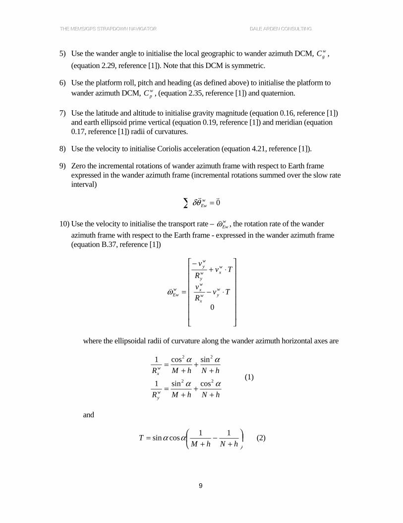
9) Zero the incremental rotations of wander azimuth frame with respect to Earth frame expressed in the wander azimuth frame (incremental rotations summed over the slow rate interval)

0vv

=∑ wEwθδ

10) Use the velocity to initialise the transport rate – wEwωv , the rotation rate of the wander

azimuth frame with respect to the Earth frame - expressed in the wander azimuth frame (equation B.37, reference [1])

⎥⎥⎥⎥⎥⎥⎥

⎦

⎤

⎢⎢⎢⎢⎢⎢⎢

⎣

⎡

⋅−

⋅+−

=

0

TvRv

TvRv

wyw

x

wx

wxw

y

wy

wEwωv

where the ellipsoidal radii of curvature along the wander azimuth horizontal axes are

hNhMR

hNhMR

wy

wx

++

+=

++

+=

αα

αα

22

22

cossin1

sincos1

(1)

and

⎟⎠⎞⎜

⎝⎛

+−

+=

hNhMT 11cossin αα (2)


10

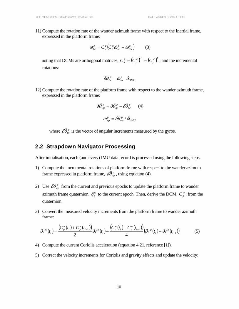
11) Compute the rotation rate of the wander azimuth frame with respect to the Inertial frame, expressed in the platform frame:

( )wEw

EIE

wE

pw

pIw CC ωωω vvv += (3)

noting that DCMs are orthogonal matrices, ( ) ( )Twp

wp

pw CCC == −1 ; and the incremental

rotations:

IMUpIw

pIw tδωθδ ⋅= vv

12) Compute the rotation rate of the platform frame with respect to the wander azimuth frame, expressed in the platform frame:

pIw

pIp

pwp θδθδθδ

vvv−= (4)

IMUp

wppwp tδθδω /

vv =

where pIpθδv

is the vector of angular increments measured by the gyros.

2.2 Strapdown Navigator Processing

After initialisation, each (and every) IMU data record is processed using the following steps.

1) Compute the incremental rotations of platform frame with respect to the wander azimuth frame expressed in platform frame, p

wpθδv

, using equation (4).

2) Use pwpθδv

from the current and previous epochs to update the platform frame to wander

azimuth frame quaternion, wpqr to the current epoch. Then, derive the DCM, w

pC , from the quaternion.

3) Convert the measured velocity increments from the platform frame to wander azimuth frame:

( ) ( ) ( )( ) ( ) ( ) ( )( ) ( ) ( )( )111

42 −−− −

−−

+= i

pi

piwpi

wp

ipi

wpi

wp

iw tvtv

tCtCtv

tCtCtv vvvv δδδδ (5)

4) Compute the current Coriolis acceleration (equation 4.21, reference [1]).

5) Correct the velocity increments for Coriolis and gravity effects and update the velocity:


11

( ) ( ) ( ) ( )( )( ) ( ) ( )i

wi

wi

w

IMUi

wCi

wCi

wi

w

tvtvtv

ttatatvtvvvv

vvvv

δ

δδδ

+=

++=

−

−

1

1 2 (6)

6) Update the transport rate, wEwωv using the updated velocity in equation B.37, reference [1].

7) Update the incremental rotations of wander azimuth frame with respect to Earth frame expressed in the wander azimuth frame (incremental rotations summed over the slow rate interval):

( ) ( )( )21

1

IMUi

wEwi

wEw

i

wEw

i

wEw

ttt δωωθδθδ vvvv++= −

−∑∑ (7)

8) Update the altitude:

( ) ( ) ( ) ( )( )211IMU

iwzi

wzii

ttvtvthth δ−− ++= vv

9) Whenever navigation output is required, prepare the output data.

A) Compute the body to wander azimuth DCM:

pb

wp

wb CCC =

where pbC is assumed constant and is dependent on and determined during IMU

installation. For a man-pack installation, pbC is simply set to the identity matrix – the

body and platform frames are defined to be coincident.

B) Extract roll, pitch and platform heading (heading with respect to the wander azimuth x-axis) from w

bC (equation 9.15, reference [1]):

( )( )

( )( ) ( )

( )( ) ⎟⎟⎠

⎞⎜⎜⎝

⎛ −=Ψ

⎟⎟

⎠

⎞⎜⎜

⎝

⎛

+=Θ

⎟⎟⎠

⎞⎜⎜⎝

⎛−−=Φ

−

−

−

1,11,2tan

1,21,1

1,3tan

3,32,3tan

1

22

1

1

wb

wbw

wb

wb

wb

wb

wb

CC

CC

C

CC

C) Update the position information as follows.


12

i) Use ∑ wEwθδv

from the current and previous epochs to update the wander

azimuth to Earth frame quaternion, Ewqr to the current epoch. Then, derive the

DCM, EwC , from the quaternion.

ii) Extract latitude, longitude and wander angle from EwC :

( )( ) ( )

( )( )

( )( ) ⎟⎟⎠

⎞⎜⎜⎝

⎛ −=

⎟⎟⎠

⎞⎜⎜⎝

⎛=

⎟⎟

⎠

⎞⎜⎜

⎝

⎛

+=

−

−

−

1,32,3tan

3,13,2tan

2,31,3

3,3tan

1

1

22

1

Ew

Ew

Ew

Ew

Ew

Ew

Ew

CC

CC

CC

C

α

λ

φ

(8)

iii) Reset 0vv

=∑ wEwθδ

D) Use the latitude and altitude to compute gravity magnitude (equation 0.16, reference [1]) and earth ellipsoid prime vertical (equation 0.19, reference [1]) and meridian (equation 0.17, reference [1]) radii of curvatures.

E) Compute true heading

α−Ψ=Ψ w

F) Compute roll, pitch and heading rates as follows.

i) Differentiate equation 2.35, reference [1], wbC (only three elements are

needed):

⎥⎥⎥⎥⎥⎥⎥⎥⎥

⎦

⎤

⎢⎢⎢⎢⎢⎢⎢⎢⎢

⎣

⎡

−Φ⋅ΘΦ−

Θ⋅ΘΦΘ⋅Θ

−−Θ⋅ΨΘ+

Ψ⋅ΨΘ−

−−−

=

&

&&

&

&

&

coscossinsin

cos

sinsincoscos

w

ww

wbC

ii) Calculate wbC& using equation 0.31 of reference [1]:


13

( )

⎥⎥⎥⎥⎥⎥⎥⎥⎥

⎦

⎤

⎢⎢⎢⎢⎢⎢⎢⎢⎢

⎣

⎡

−ΘΦ⋅−

Θ⋅−ΘΦ⋅+ΘΦ⋅−

−−ΨΦ−ΨΘΦ⋅+

ΨΦ−ΨΘΦ−⋅

−−−

=×=

coscossin

coscoscossin

)cossinsinsin(cos)coscossinsinsin(

x

z

y

z

wwy

wwz

bwb

wb

wb CC

ωω

ωω

ωω

ωv&

where ⎥⎥⎥

⎦

⎤

⎢⎢⎢

⎣

⎡=

z

y

xbwb

ωωω

ωv (computation procedures detailed below).

iii) Equate the (3,1) terms to get the pitch rate in terms of roll, pitch, heading and bwbωv :

Φ⋅−Φ⋅=Θ sincos zy ωω&

iv) Equate the (3,2) terms to get the roll rate in terms of roll, pitch, heading and bwbωv :

ΘΦ⋅−Θ⋅−=Φ⋅ΘΦ−Θ⋅ΘΦ coscossincoscossinsin xz ωω&&

(a) Substitute the expression just derived for the pitch rate to get

ΘΦ⋅−Θ⋅−=Φ⋅ΘΦ−ΘΦ⋅−ΦΘΦ⋅ coscossincoscossinsincossinsin 2xzzy ωωωω &

(b) Solve for the roll rate

( )1sinsincossinsincoscos

coscossinsinsincossinsincoscos2

2

−ΦΘ⋅−ΦΘΦ⋅+ΘΦ⋅=

ΘΦ⋅+Θ⋅+ΘΦ⋅−ΦΘΦ⋅=Φ⋅ΘΦ

zyx

xzzy

ωωω

ωωωω&

ΦΘ⋅+ΘΦ⋅+Θ⋅=Φ⋅Θ cossinsinsincoscos zyx ωωω&

ΘΦ⋅+ΘΦ⋅+=Φ tancostansin zyx ωωω&


14

v) Equate the (2,1) terms to get the heading rate in terms of roll, pitch, heading and b

wbωv :

)cossinsinsin(cos)coscossinsinsin(

sinsincoscos

wwy

wwz

www

ΨΦ−ΨΘΦ⋅

+ΨΦ−ΨΘΦ−⋅=Θ⋅ΨΘ+Ψ⋅ΨΘ−

ωω

&&

(a) Substitute the expression derived for the pitch rate and rearrange:

( )

)cossinsinsin(cos

)coscossinsinsin(

sincossinsincoscos

wwy

wwz

zyw

ww

ΨΦ−ΨΘΦ⋅

−ΨΦ−ΨΘΦ−⋅

−Φ⋅−Φ⋅ΨΘ

=Ψ⋅ΨΘ

ωω

ωω

&

(b) Simplify to

)cossin()coscos(coscos

wy

wz

ww

ΨΦ−⋅−ΨΦ−⋅=Ψ⋅ΨΘ

ωω

&

Φ⋅−Φ⋅=Ψ⋅Θ cossincos zyw ωω&

(c) And solve for platform heading rate:

ΘΦ⋅−Φ⋅

=Ψcos

cossin zyw ωω&

vi) Compute bwbωv as follows:

(a) bwp

bpb

bwp

bwb θδθδθδθδ

vvvv=+= , assuming the IMU is rigidly attached to the

body (i.e. 0vv

=bpbθδ ).

(b) Then, pwp

bp

bwb C θδθδ

vv= .

(c) And, IMUb

wbbwb tδθδω /

vv = .

vii) Compute the true heading rate by subtracting the wander angle rate from the platform heading:

α&&& −Ψ=Ψ w


15

where the wander angle rate, α& , is given in equation B.59 of reference [1].

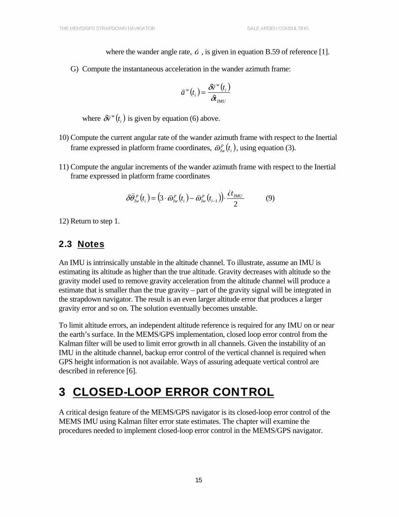
G) Compute the instantaneous acceleration in the wander azimuth frame:

( ) ( )IMU

iw

iw

ttvta

δδvv =

where ( )iw tvvδ is given by equation (6) above.

10) Compute the current angular rate of the wander azimuth frame with respect to the Inertial frame expressed in platform frame coordinates, ( )i

pIw tωv , using equation (3).

11) Compute the angular increments of the wander azimuth frame with respect to the Inertial frame expressed in platform frame coordinates

( ) ( ) ( )( )2

3 1IMU

ipIwi

pIwi

pIw

tttt δωωθδ ⋅−⋅= −vvv

(9)

12) Return to step 1.

2.3 Notes

An IMU is intrinsically unstable in the altitude channel. To illustrate, assume an IMU is estimating its altitude as higher than the true altitude. Gravity decreases with altitude so the gravity model used to remove gravity acceleration from the altitude channel will produce a estimate that is smaller than the true gravity – part of the gravity signal will be integrated in the strapdown navigator. The result is an even larger altitude error that produces a larger gravity error and so on. The solution eventually becomes unstable.

To limit altitude errors, an independent altitude reference is required for any IMU on or near the earth’s surface. In the MEMS/GPS implementation, closed loop error control from the Kalman filter will be used to limit error growth in all channels. Given the instability of an IMU in the altitude channel, backup error control of the vertical channel is required when GPS height information is not available. Ways of assuring adequate vertical control are described in reference [6].

3 CLOSED-LOOP ERROR CONTROL A critical design feature of the MEMS/GPS navigator is its closed-loop error control of the MEMS IMU using Kalman filter error state estimates. The chapter will examine the procedures needed to implement closed-loop error control in the MEMS/GPS navigator.


16

3.1 The Purpose of Closed-Loop Error Control

The advantages of IMU/GPS integration have long been recognised. Significant benefits can be gained by an external Kalman filter that combines IMU and GPS data such as

In-flight calibration of IMU sensor errors,

Low noise, bounded navigation errors.

The additional advantages of so-called tightly coupled IMU/GPS systems were soon being promoted. These included:

In-flight IMU alignment (and re-start), requiring access to the internal IMU navigation processor;

Enhanced GPS anti-jam capabilities, requiring access to the internal GPS navigation processor.

Tightly coupled IMU/GPS use closed loop error control to feed Kalman filter error estimates back to the IMU and GPS sensors, effectively reducing sensor errors. Practical systems were not possible until GPS receiver size, weight, and power consumption could be adequately reduced.

As early as 1988, tightly coupled, Embedded GPS/INS (EGI) systems were proposed (e.g. reference [4]). Motivation for early EGIs was derived to some degree by the desire to install GPS in military aircraft without the large expenditures required of a standalone installation in limited avionics space. “Embedding” the GPS inside an existing INS chassis would provide savings in space, power consumption, weight, cooling, etc. versus a standalone GPS installation. Of course, the desire to install GPS was motivated by the performance improvements it provided, especially when combined with an inertial system. The EGI format also provided an environment that was conducive to tight coupling. For example, measurements of encrypted pseudorange messages made by military receivers cannot be exported outside of the physical box containing the receiver. An EGI, with the IMU and GPS receiver in the same box can use encrypted pseudoranges directly. Conversely, an integrated system with IMU and GPS in separate boxes, connected by cabling, cannot use encrypted pseudoranges - it is restricted to the use of GPS positions, velocities (and sometimes attitude).

The MEMS/GPS system described in this report is really an ancestor of these early EGI systems. The challenge in 1988 involved reduction of GPS receiver size to a single circuit board. Today the challenge is performance enhancements for accelerometers, gyros and GPS receivers that each fit onto a single silicon chip. In 1988, the standard DOD receiver 3A with its mount weighed about 20 kg. Today a full 3-D IMU can weigh as little as 0.25 kg.

Since 1988, while GPS receivers were shrinking from kilograms to grams, their performance was actually increasing. This feat required enormous effort from many contributors, even though, as RF devices, GPS receivers might be considered more amenable to miniaturisation.


17

Miniaturisation of inertial sensors is in some ways more challenging but has not enjoyed the level of effort put into GPS developments. As a result, miniature inertial sensors are much less accurate than their larger counterparts. MEMS inertial sensors are an integration of miniature mechanical structures, sensors, actuators, and electronics on a common silicon (and sometimes quartz) substrate. They are built using batch fabrication techniques (similar to IC processes) that provide high levels of functionality, reliability, and sophistication on a small silicon chip at a relatively low cost. A typical MEMS gyro consists of a vibrating mass driven by a piezoelectric device. An inertial rotational input produces a Coriolis force that is measured by the sensor. A MEMS accelerometer may be a suspended proof mass that responds to an input acceleration by transferring a force to its supports, or it might be a vibrating mass whose vibrational characteristics change under the influence of an input acceleration. The magnitude of MEMS inertial sensor outputs is proportional not only to the magnitude of the sensed input but also to the mass of sensing element. For example, the force exerted by a proof mass under acceleration is equal to its mass multiplied by the acceleration. The tiny mass of a MEMS sensor results in tiny output signals. The first challenge involves accurate measurement of these tiny signals. Then measurements must be processed so they can be output in a useable form. The electronic noise associated with the signal collection and processing is a major contributor to a MEMS error budget. Even things like the Brownian motion of the air molecules around the sensor introduce measurable errors.

Recall that inertial sensor outputs are integrated to produce navigation outputs. These large MEMS sensor errors are integrated along with the inertial signal, resulting in navigation solutions that quickly become unstable without some kind of mitigation strategy. Integration of a MEMS IMU with GPS and other aiding sensors provides an excellent environment for such strategies. Corrections to navigation quantities can be provided by the integrated Kalman filter solution or directly from the aiding sensors when the filter is judged to be unreliable. This process serves to limit the absolute IMU navigation errors. Further, the Kalman filter produces estimates of inertial sensor errors. These estimates, when fed back to the IMU, will reduce the rate of IMU error growth. An IMU calibrated in this way will be able to navigate successfully for periods of time (far?) exceeding an uncalibrated unit.

The best MEMS production gyros currently have specifications on the order of 100 degrees per hour turn-on to turn-on biases and 5 to 25 degrees per hour in-run biases. The best accelerometers exhibit turn-on to turn-on biases in the range of 2 to 10 millig’s and in-run biases of 30 microg’s to 2 millig’s. The larger repeatable biases and smaller in-run biases also fit well with the MEMS/GPS integration concept:

At turn-on, the IMU with exhibit large sensor biases composed of a large random constant term plus a smaller random drifting term.

As the filter starts processing measurements from the aiding sensors, it begins to estimate the sensor biases.

These estimates are fed back to the IMU, which corrects its sensor outputs accordingly.


18

Over time, the filter estimates will improve and the IMU will become better calibrated.

Now assume that all aiding measurements are lost. The constant part of the sensor bias estimates will remain fixed at the last pre-loss value. The drift component of the estimates will slowly degrade, approaching zero asymptotically. The rate of degradation will depend on the characteristics of the particular sensors.

So a short time after the loss of measurements, the IMU will be fully calibrated with good estimates of both the constant and drifting bias components (of course, the sensor errors will never be perfectly known). Some time later, the drift bias estimates will be degraded. Eventually, they will have no useful effect on IMU performance. However, the larger, constant bias estimates will continue to provide useful calibration information to the IMU right up to the time it powered down. Of course, any subsequent measurements will again serve to improve both components of the bias estimate.

3.2 The MEMS/GPS Error Control Process

The previous section described the rationale behind IMU error control and briefly described the process. In this section, the details of the MEMS/GPS closed loop error control process will be laid out. It will be logically split into navigation error control (navigator reset) and sensor error control (calibration).

The MEMS/GPS Kalman filter uses the IMU data as its basis. Information from independent aiding sensors is compared to corresponding IMU data to form filter measurements. The measurements are used in a stochastic model to update (improve) the estimates of the errors in the filter’s state vector. The observability of individual states depends on the specific measurements, error models, trajectory, etc. Measurements are processed at specific time epochs. Between measurement epochs, a complex IMU error model is used to propagate the state estimates forward in time. In general, state uncertainty increases as a function of time since the last update epoch.

Normally, aiding sensor data arrives and is processed at regular rates. Occasionally, data records will be missed or corrupted. The MEMS/GPS Kalman filter package has been designed to detect and properly deal with these kinds of data deficiencies. When the time between updates is larger than normal, the filter simply continues to propagate its last updated state vector, with state variance estimates generally growing larger with time. When the next good measurements arrive, they will be processed and will again drive variances down. Typically, a saw-tooth pattern is observed: errors grow slowly between updates, and then immediately decrease in response to a new update. The general trend will be one of decreasing variances early in a run, then fairly constant variances once steady state is reached. Sporadic losses of measurement data will not disturb this trend, provided update intervals are much shorter than error correlation times (this is the usual situation in modern integrated navigation systems where update intervals are on the order of one second). However, sustained interruptions in aiding data will cause state variances to begin an upward trend. One major goal of the MEMS/GPS project is the development of techniques that can be employed


19

to slow the rate of growth of errors after GPS is lost (due to signal jamming or attenuation). Specifically, the goal is maximization of the time required to reach a given acceptable maximum navigation error after a loss of GPS. Time to failure will be maximised when the rate of error growth is minimised. Two strategies will be employed:

All possible non-GPS measurement data will be processed. In general, a particular measurement will limit the error in the corresponding state estimate. At the same time, the rates of growth of other state estimates can be slowed (see the comment on observability above). Non-GPS measurements will include sensor data like digital compass heading and possibly altitude from a baro-altimeter. Non-sensor velocity data can also be used to form measurements. For example, the operator can stop and maintain zero velocity. Zero velocity measurements can then be processed in the filter. On a wheeled vehicle, velocity perpendicular to the direction of travel can be assumed to be zero even when the vehicle is moving. Again, this information can be used update the filter.

Closed loop error control will be employed to limit the size of the IMU navigation errors and to limit the rate of growth when measurements are lost.

Closed loop error control is the topic of interest here. In brief, closed loop error control limits the size and growth rates of IMU errors by feeding Kalman filter estimates of IMU navigation and sensor errors back to the IMU: the navigation error estimates are used to correct the corresponding navigation parameters in the strapdown navigator; the sensor error estimates are used to correct the IMU measurements prior to their integration in the strapdown navigator.

The process will be discussed in detail in the following sections.

3.2.1 Development and Analysis of Closed Loop Error Control

The MEMS/GPS Kalman filter uses measurements from aiding sensors to derive estimates of IMU navigation errors and IMU sensor errors. As discussed above, those Kalman filter error estimates can be used as corrections in the strapdown navigator. In this section, the details of the Kalman filter error control procedures will be presented.

3.2.1.1 Normal Operation

The use of closed loop error control has an impact on the operation of the Kalman filter: correction of IMU parameters requires a like correction to the corresponding filter states. For example, let’s assume that there is a Kalman filter estimate of IMU latitude error of 100 metres. That estimate is sent to the strapdown navigator where the latitude is corrected. The true IMU latitude error has now been adjusted by 100 metres. The Kalman filter’s estimate of the true latitude error must also be corrected by the same 100 metres (this is analogous to a control input).


20

While it is useful to have the closed loop error corrections applied in the strapdown navigator as soon as possible after they have been estimated in the filter, it is critical that the filter states applicable to the exact instant of the reset be corrected by the same values used in the navigator. To illustrate this point, consider, what appears to be, a obvious filter error control procedure:

1. Collect and process measurements from the aiding sensors to produce updated error state estimates.

2. Immediately send the updated error estimates to the strapdown navigator to be used for error control.

3. Reset the states used for error control to zero (the current state estimate minus the value used for error control).

4. If all the states are used for error control (and thus zeroed), there is no need to propagate the state vector (in the Kalman filter process, a zero length-state vector will always propagate to the same zero-length state vector).

At first glance, this seems perfectly fine. However, there is a subtle problem. The state estimates produced by the filter update actually apply to the instant of time at which the measurements are valid. During the finite length of time needed to actually perform the filter update, the IMU errors have changed. The updated error estimates (applicable to the aiding data epoch) are sent to the strapdown navigator for error control. Even if the error control data were perfect, the remaining IMU errors will not be zero; they will be equal to the change in the errors over the time interval from the update epoch to the time the error control was applied. Resetting the filter’s error control states to zero, neglects these small IMU error changes.

Let’s use the example above to illustrate this problem. Assume IMU latitude for epoch ti , with an error of 100 metres, is sent to the filter and used for an update. In practice, the aiding sensor data is inter(extra)-polated to time ti to form measurements. At time ti+1, the filter update based on these measurements is complete. For simplicity, assume that the filter was able to perfectly estimate the latitude error at time ti , and a latitude correction of 100 metres is sent to the navigator and used for error control. But, by time ti+1, the IMU latitude error (before error control) has in fact grown to101 metres. After correction, there is a 1-metre error remaining in the IMU latitude. Now if the filter’s latitude error is zeroed at time ti+1, this is actually a correction of 101 metres; not the 100-metre correction sent to the strapdown navigator. The IMU’s true latitude error has been corrected by 100 metres; the filter has been corrected by 101 metres. If the filter knew that it had produced a perfect latitude error estimate (not a realistic prospect), it would assign an uncertainty of zero to its latitude error estimate. But, the 1 metre error introduced by zeroing the latitude state is not reflected in the filter’s uncertainty (i.e. the latitude variance). This incongruity can lead stability problems.

Of course, the faster the IMU errors change, the bigger the problem. If the latitude error in the above example increased by 10 metres between ti and ti+1, the effects on the filter would be


21

much more severe. And, error growth rates of the MEMS IMUs used in this project can indeed by very high.

So, what is to be done? The answer is quite simple:

1. Form the measurements at time ti, as usual (the IMU data used to form the measurements have not been corrected).

2. Send the most recent estimates of the error control states to the strapdown navigator (the estimates propagated to the current update epoch).

3. Save the selected state vector.

4. As soon as the error control information arrives at the strapdown navigator, apply it to the IMU data.

5. Proceed with the filter update to get estimates of the states at time ti.

6. Reset the updated state vector at ti using exactly the same error estimates that were used for error control.

Back to our example.

1. Form the latitude measurement at time ti.

2. Send the strapdown navigator the estimate of the latitude error state propagated to ti (assume a value of 99 metres – a 1-metre propagation error).

3. Save the latitude state.

4. As soon as the latitude error information arrives at the strapdown navigator, apply it to the IMU data (reducing the latitude error by 99 metres).

5. Proceed with the filter update to get estimates of the latitude error at time ti (we assumed 100 metres).

6. Reset the updated latitude error state at ti using exactly the 99 metres that was used for error control (resulting in a post-reset latitude error of 1 metre). The strapdown navigator and the Kalman filter have both been corrected by the same amount. Continuing with the earlier assumptions, the filter thinks its estimate of IMU latitude error (1 metre) is perfect. And the true IMU latitude error is in fact 1 metre (the true error at ti was 100 metres; 99 metres of that was removed during error control). The filter is consistent with the true IMU errors!

As will be discussed in the next section, the consistency sought does really require equivalency between the true error and the state estimate. It requires that the difference between the two be properly estimated by the state’s variance. The Kalman filter process


22

propagates and updates its state vector plus the covariance matrix associated with that state vector. In this example, the requirement of zero difference implies that the latitude state’s variance after update must be zero (or very small).

3.2.1.2 Degraded Operation

The proper error control procedures for normal filter operation have been described. Are these procedures able to deal with degraded filter operation? What if the measurement contains a blunder that causes it to be rejected in the filter’s residual testing algorithms? What if measurements are lost for some length of time? Or if certain measurements are lost, but some are retained: if position measurements are lost, should IMU positions be corrected with the filter’s position states?

Let’s begin the analysis by looking at the effect of one lost measurement using the standard procedures described in the last section. Steps 1 to 4 proceed as before. But, in Step 5, the measurement fails so the state vector is not updated. If the latitude error is reset in Step 6, the state will be reduced to zero. Is this consistent with the IMU? After all, the true IMU error is 1 metre after error control, while the state estimate is zero. The answer is provided by the Kalman filter’s ability to propagate and update not just its states, but also estimates of its states accuracy. In this example, since the measurement update failed, the filter’s estimate of latitude variance was not updated (to the very small number described in the previous section), but continued to grow. Assuming the variance propagation model is correct, the 1-metre difference between the true latitude error and the filter’s estimate will be properly modelled by the filter’s latitude variance. So once again, the filter is consistent with the true IMU error behaviour.

What if the measurement updates fail for some extended period of time – maybe GPS signals have been lost? The standard error control procedures adequately handle the first lost update. Let’s look at the second. Between the first lost update and the next, the IMU latitude error grows from 1 metre to some larger value; the filter’s latitude error estimate stays at zero (assuming no correlation with other non-zeroed states) but its variance continues to grow. Assuming a proper propagation model, the filter variance will properly reflect the difference between the true latitude error and the filter’s estimate. The measurement is formed; the latitude error state (recall that it is still zero) is sent to the strapdown navigator and applied to the IMU data (a zero-valued correction in this case). Then, the filter update proceeds but is rejected in statistical testing. The zero-valued latitude state is corrected by the zero-valued error control value, thus remaining at zero. As time progresses, IMU latitude errors continue to grow but are properly modelled by the filter’s growing variance estimates. The consistency of the filter results depends on the quality of its propagation model. In general, the quality of the model decreases with time.

So the IMU and filter have been operating for some time with no measurement updates and (effectively) no error control (this simplistic model neglects the IMU sensor error calibration). GPS signals are suddenly available, providing good latitude measurements to the filter. The next filter update epoch arrives. What happens to the error control procedures? First, the propagated latitude error state is still zero; so the error control correction is zero. The


23

measurement is successfully processed and the update succeeds: a (probably large) latitude error state is estimated along with a much reduced latitude variance (roughly equal to the estimated accuracy of the GPS latitude). The zero-valued state reset does not change the state estimate. At this point, there is a large IMU latitude error, a large filter latitude error estimate and a small latitude variance. The variance is estimating the expected error in the latitude error state – the difference between the true error and the filter’s error estimate. If the GPS latitude accuracy estimate was correct, the filter should still be consistent. The large latitude error state will be propagated to the next update epoch, and then it will be sent to the strapdown navigator for error control. Now the large IMU latitude error will be greatly reduced. The update will proceed; the latitude error state will be reset. Now there is a small IMU latitude error, a small filter latitude error estimate and a small latitude variance. Again, everything seems consistent.

These are the most common degraded modes. However, this analysis assumed that the filter’s propagation model accurately describes the true IMU error growth characteristics. The filter designer must take great care to ensure that the model implemented is adequate. Kalman filter implementations always involve trade-offs between complexity and practicality. If errors capable of producing significant IMU errors are not properly modelled, problems will arise. And sometimes, IMU sensor errors will suddenly change. These changes can sometimes be detected but cannot be easily modelled. It is believed that the solid-state MEMS sensors used for this project are unlikely to exhibit such changes in performance: they will likely operate to specifications or not operate at all.

3.2.1.3 Conclusion

It seems that the error control procedure as described will maintain filter consistency and stability through normal and (at least the most common) degraded operation modes.

3.2.2 Implementation of Closed Loop Error Control

To begin discussing implementation details, we’ll have to leave our simplistic one-state system behind. The realistic system to be discussed in this section will be comprised of a large number of states, and those states will be divided into two distinct groups.

The “system” states describe IMU navigation errors – position, velocity and attitude.

The “sensor” states describe IMU sensor errors – accelerometer and gyro biases and perhaps other errors.

These two groups are not distinguished in the Kalman filter side of error control: all states are propagated to the update epoch, all (IMU) states are sent to the strapdown navigator, all states are updated, and all (IMU) states are reset. However, once the error control states reach the strapdown navigator, they are separated and used in very different ways.


24

3.2.2.1 System States in the Strapdown Navigator

The latitude error used in the example in the previous section would be classified a system state. All the members of the complete set of system states found in real system are dealt with in essentially the same fashion: the error control system states are used to correct the corresponding IMU navigation parameters. However, in practice, it is not normally as simple as adding the latitude error estimate to the IMU-computed latitude. For example, the MEMS/GPS Kalman filter implements all system states in the wander azimuth frame. Fortunately, the strapdown navigator operates in the same frame, simplifying the error control procedures.

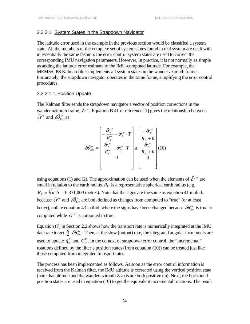
3.2.2.1.1 Position Update

The Kalman filter sends the strapdown navigator a vector of position corrections in the wander azimuth frame, wrδ

v. Equation B.41 of reference [1] gives the relationship between

wrδv

and wEwθδv

as

⎥⎥⎥⎥⎥⎥⎥

⎦

⎤

⎢⎢⎢⎢⎢⎢⎢

⎣

⎡

+

+−

≅

⎥⎥⎥⎥⎥⎥⎥

⎦

⎤

⎢⎢⎢⎢⎢⎢⎢

⎣

⎡

⋅−

⋅+−

=

00hR

rhR

r

TrRr

TrRr

E

wx

E

wy

wyw

x

wx

wxw

y

wy

wEw

δ

δ

δδ

δδ

θδv

(10)

using equations (1) and (2). The approximation can be used when the elements of wrδv

are small in relation to the earth radius. RE is a representative spherical earth radius (e.g.

3 2baRE = = 6,371,000 metres). Note that the signs are the same as equation 41 in ibid. because wrδ

v and w

Ewθδv

are both defined as changes from computed to “true” (or at least better), unlike equation 43 in ibid. where the signs have been changed because w

Ewθδv

is true to computed while wrδ

v is computed to true.

Equation (7) in Section 2.2 shows how the transport rate is numerically integrated at the IMU data rate to get ∑ w

Ewθδv

. Then, at the slow (output) rate, the integrated angular increments are

used to update Ewqr and E

wC . In the context of strapdown error control, the “incremental” rotations defined by the filter’s position states (from equation (10)) can be treated just like those computed from integrated transport rates.

The process has been implemented as follows. As soon as the error control information is received from the Kalman filter, the IMU altitude is corrected using the vertical position state (note that altitude and the wander azimuth Z-axis are both positive up). Next, the horizontal position states are used in equation (10) to get the equivalent incremental rotations. The result


25

is added to the current sum, ∑ wEwθδv

. Then, the position update procedures of steps (9)C) and (9)D) in Section 2.2 are executed:

1) Use ∑ wEwθδv

(all IMU contributions up to the current time plus the position correction

contribution) to update Ewqr .

2) Derive the DCM, EwC , from the quaternion.

3) Extract updated values of latitude, longitude and wander angle from EwC using equation

(8)

4) Reset 0vv

=∑ wEwθδ

5) Use the new latitude and altitude to update gravity magnitude, prime vertical and meridian radii of curvatures.

3.2.2.1.2 Attitude Update

Updating the IMU’s roll, pitch and heading is a bit less direct than the position update. To begin, an explanation of the information being sent from the Kalman filter to the navigator is required. In brief, there are two error formulations most often used in a Kalman filter such as the one used here: or formulations. The terminology refers to the definition of the attitude errors used.

Three, very similar, wander azimuth coordinate frames have to be described before continuing:

1. The “platform” frame has its orientation determined by the IMU measurements and its origin at the IMU-computed position (it is the strapdown navigator’s wander azimuth frame).

2. The “true” frame is the perfectly local level frame with its origin at the IMU’s true position.

3. The “computer” frame is the perfectly local level frame with its origin at the IMU-computed position.

Three sets of small angles define the rotations between these frames:

1. ψv is the rotation vector from the computer to platform frame.

2. ϕv is the rotation vector from the true to platform frame.


26

3. ϑδv

is the rotation vector from the true to computer frame.

4. It follows that ψϑδϕ vvv += .

The DCMs between frames, using the small angle approximations 1cos ≅δ and δδ ≅sin are given as

1. ( )×−= ψvIC pc

2. ( )×−= ϕvIC pt

3. ( )×−= ϑδv

IC ct

The - and -formulations alluded to above refer to the rotation vector estimated in the Kalman filter. More details are available in reference [1].

In the strapdown navigator, the platform frame to wander azimuth frame quaternion (DCM) defines the IMU attitude. Note that the platform frame defined by the orthogonal approximation to the accelerometers’ sensitive axes will be called the body frame in these discussions to avoid confusion with wander azimuth platform frame just defined. Attitude error control must correct w

bqr and wbC using Kalman filter error state estimates. The solution

can be described in terms of DCM corrections or quaternion corrections.

3.2.2.1.2.1 DCM Correction The DCM solution is a bit more straightforward; so let’s start there. Keep in mind the fact that the platform, true and computer frames are all variations of the wander azimuth frame. Now, the body frame to wander azimuth DCM before error control can be written p

bC . Error control should provide the best estimate of t

bC . This is easily accomplished using

( ) pb

pb

tp

tb CICCC ×+== ϕv

If the -angles are supplied by the Kalman filter, ϕv can be directly plugged in to this equation to provide t

bC .

However, if the -angles are supplied by the Kalman filter, ϕv must be computed as follows. The discussions above showed that ψϑδϕ vvv += where ψv comes directly from the filter and

ϑδv

can be computed using the position error states. In fact, this has already been done in equation (10) in the position update section. After ϕv has been computed, it can be used to provide t

bC . Then, the updated quaternion would be derived from tbC .


27

3.2.2.1.2.2 Quaternion Correction As the IMU moves and rotates, attitude is maintained and updated in the strapdown navigator via the body frame to (platform) wander azimuth frame quaternion, specifically p

bqv . This quaternion is updated at the IMU data rate using b

wbθδv

as computed in equation (4) (note the notation change – p now identifies the wander azimuth platform frame and b identifies the body frame (w and p, respectively, were used in equation (4)).

In step 2) of the strapdown processing of Section1 2.2, the body frame to wander azimuth frame quaternion ( w

bqr ) update was performed with a small rotation vector ( bwbθδv

). The -angles can be interpreted as small rotations of the wander azimuth frame with respect to the body frame evaluated in the wander azimuth frame ( w

bwθδv

). Note that the -angles are rotations from true to platform frames. However, to update w

bqr with the Kalman filter error state estimates, the platform to true rotations are required, the negative of the -angles:

( ) ϕθδ vv−=KFw

bw

To use the -angles to get the bwbθδv

required for the body to wander azimuth quaternion update, begin by changing the sign:

( ) ϕθδ vv=KFw

wb

Then rotate ( )KFwwbθδv

into the body frame:

( ) ( )KFCKF wwb

bw

bwb θδθδ

vv=

The resulting rotation vector, ( )KFbwbθδv

, is then used to update the quaternion from pbqr to t

bqr , using the same algorithm used in Section1 2.2.

The DCM, tbC , is derived from t

bqr using standard methods.

3.2.2.1.2.3 Note on Attitude Updates The DCM attitude update was originally programmed into the MEMS/GPS software system. However, it was discovered that this procedure was unstable under certain conditions. Note that the small angle approximations used in the DCM update contradict a basic DCM attribute, that of normality: the norm (length) of each row and column vector comprising the DCM should equal one. The norm of a quaternion should always be equal to one. An approximate DCM like ( )×−= ϕvIC p

t clearly violates this rule. However, if ϕv is small enough, the error is assumed negligible.

For unknown reasons, the DCM implementation occasionally produced quaternions with norms much larger than one (as large as 10). At these times, large tilts were introduced. These


28

tilts led to spikes in height error. It was the height instability that first drew attention to the problem. These problems did not necessarily arise when Kalman filter tilt errors were largest, they were unpredictable and generally not reproducible.

Rather than attempting to (perhaps futilely) identify the root cause of the problems with the DCM attitude reset, it was replaced by the quaternion-reset procedure. Extensive testing confirmed that the attitude resets are now stable.

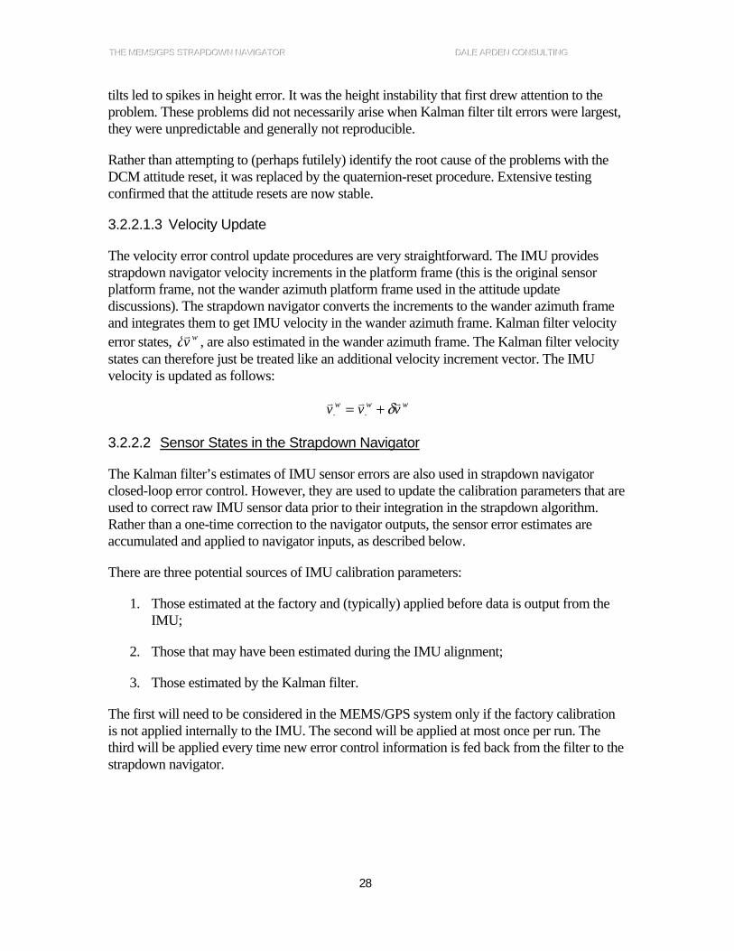
3.2.2.1.3 Velocity Update

The velocity error control update procedures are very straightforward. The IMU provides strapdown navigator velocity increments in the platform frame (this is the original sensor platform frame, not the wander azimuth platform frame used in the attitude update discussions). The strapdown navigator converts the increments to the wander azimuth frame and integrates them to get IMU velocity in the wander azimuth frame. Kalman filter velocity error states, wvvδ , are also estimated in the wander azimuth frame. The Kalman filter velocity states can therefore just be treated like an additional velocity increment vector. The IMU velocity is updated as follows:

www vvv vvv δ+= −+

3.2.2.2 Sensor States in the Strapdown Navigator

The Kalman filter’s estimates of IMU sensor errors are also used in strapdown navigator closed-loop error control. However, they are used to update the calibration parameters that are used to correct raw IMU sensor data prior to their integration in the strapdown algorithm. Rather than a one-time correction to the navigator outputs, the sensor error estimates are accumulated and applied to navigator inputs, as described below.

There are three potential sources of IMU calibration parameters:

1. Those estimated at the factory and (typically) applied before data is output from the IMU;

2. Those that may have been estimated during the IMU alignment;

3. Those estimated by the Kalman filter.

The first will need to be considered in the MEMS/GPS system only if the factory calibration is not applied internally to the IMU. The second will be applied at most once per run. The third will be applied every time new error control information is fed back from the filter to the strapdown navigator.


29

3.2.2.2.1 Factory Calibration Parameters

If factory calibration parameters are available but are not applied prior to IMU sensor data output, they will be applied in MEMS/GPS at the data collection level. This will allow the use of the same sensor calibration procedures for all IMU models (i.e. the strapdown navigator does not need know which IMU model it is processing).

3.2.2.2.2 Alignment Calibration Parameters

Certain alignment procedures will allow estimates of some IMU error parameters (e.g. accelerometer biases using the alignment process described in reference [5]). If the alignment does provide IMU error estimates, those estimates are used to initialise the strapdown navigator’s IMU calibration variables.

3.2.2.2.3 Kalman Filter Calibration Parameters

The MEMS/GPS error control process works in a closed-loop fashion:

IMU data is sent to the Kalman filter where IMU errors are estimated.

The error estimates are sent to the strapdown navigator.

The Kalman filter estimates are reduced by the same amount.

This process is followed for IMU sensor error estimates as well as navigation errors. The filter is expecting that all future IMU data it receives will be corrected for the all past error estimates. In the case of the system (or navigation) error control described in the previous section, the Kalman filter error estimates, being applied to integrated parameters, are accumulated implicitly. Sensor error control is applied to the integrands and therefore must be explicitly summed (integrated).

When the strapdown navigator is started, the sensor calibration parameters are initialised. If errors were estimated during alignment, they are used; otherwise the sensor calibration parameters are initialised to zero. Recall that factory calibrations will have been applied prior to the data’s arrival at the strapdown navigator.

Immediately after arriving at the strapdown navigator, each IMU data record is corrected using the current sensor calibration parameters. The calibrated IMU data is then processed in the strapdown navigator and sent off to the Kalman filter. The filter estimates the sensor errors remaining after calibration and sends these back to the navigator. Since these are estimates of the errors remaining after calibration, they are added to the current calibration parameters. The updated calibration parameters are used to correct subsequent IMU data, and the process repeats.

In a hypothetical IMU with constant errors, the calibration parameters would converge to the constant errors while the filter’s sensor error estimates would converge to zero.


30

In a realistic MEMS IMU, we expect the calibration parameters to track the true (changing) sensor errors with some time delay (depending on the filter model, measurements used, etc.). What happens under this process when Kalman filter measurements are lost?

The process used in the MEMS/GPS system is summarised in Section 3.2.1.1. Section 3.2.1.2 describes the operation of the Kalman filter after loss of good aiding sensor data. Let’s look at the strapdown navigator after loss of filter updates.

The analysis in Section 3.2.1.2 is a bit too simplistic for the present needs. There, latitude was analysed as if it were the only state being estimated. Loss of the latitude measurement led to a zeroing of the latitude state until measurements resumed. In a real filter, the latitude error state is correlated to and driven by velocity, attitude and IMU sensor error states. If any of these correlated states is non-zero, it will drive the latitude state away from zero during the filter propagation step. Recall that the states propagated to the time immediately prior to measurement processing are sent to the strapdown navigator for error control.

If measurements are successfully processed, the states will be updated and then reset to the difference between the pre- and post-update error estimates. In general, the reset states will not be zero. Therefore, after the next propagation step, (to continue our example)

The latitude error state estimate will not (in general) be zero (with contributions from the non-zero latitude error at the start of the propagation interval plus the non-zero correlated states).

All error control states will be used to correct their respective IMU parameters. IMU sensor error states will be added to the previous calibration parameters.

If the latitude state cannot be updated, it will be precisely zeroed at the state reset step (since the pre- and post-update error estimates are identical). If all correlated states are included in the error control process, they will also all be zeroed. In this case, after the next propagation step,

The latitude error state estimate will remain at zero.

None of the IMU error control parameters will be changed. The IMU sensor calibration values will remain constant so long as filter measurements are unavailable.

Is this an acceptable result? That the IMU sensor errors are assumed to be constant? At present, all indications suggest that this will not be a problem:

MEMS inertial sensors biases are typically characterised by large run-to-run errors plus smaller in-run errors.

Time intervals with no aiding measurements are expected to be short relative to the correlation times of the sensor errors.


31

After measurements are lost, the strapdown navigator will continue processing with the calibration parameters estimated at the last filter update time. As time progresses, the in-run IMU sensor errors will slowly change. This results in an unavoidable discrepancy between the modelled and true errors. Without new measurements, there is no better estimate of the sensor errors than that being used for IMU calibration. Given relatively short measurement outages and slowly varying errors, acceptable IMU performance is expected. At present, the rate of change of the so-called in-runs errors is not known. Future laboratory analysis of MEMS IMUs with a range of accuracies will provide a better understanding of expected characteristics. The error rates of change will, to a large degree, determine the length of time that can be adequately bridged without measurements.

Let’s take a look at the Kalman filter’s behaviour. As mentioned, all IMU states will be zeroed after all measurements are lost. However, the filter’s state accuracy estimates (the state covariance matrix) will continue to propagate according to the a priori model. In general, the filter predicted accuracy would decrease as a function of the propagation time interval – the length of time that has passed since the last successful measurement update. Note that some inertial errors propagate periodically (mainly with 84 minute and 1 day periods).

4 SUMMARY The preceding report has described the strapdown navigator used in the MEMS/GPS project. A strapdown navigator is the rather complex algorithm that takes accelerometer and gyroscope data from a strapdown IMU and produces navigation (position, velocity, and attitude) output.

An IMU that is “strapped down” is rigidly attached to vehicle (for example): as the vehicle moves and rotates, the accelerometers and gyros move and rotate with it. Thus, the IMU outputs are provided in a (nominally Cartesian) coordinate frame that it is attached to the vehicle. Navigation output is required in an earth-referenced frame. The strapdown navigator is required to resolve the IMU data into changes position, velocity and attitude. In essence, the gyro data is used to measure changes in the orientation of the vehicle (body frame) with respect to an earth-fixed frame, and the accelerometer data is integrated into changes in velocity and position. Note that a dead-reckoning device like an IMU requires proper initialisation of all navigation data.

Strapdown navigator processing is complicated by motion along the curved surface of the earth: the earth-fixed frame rotates as the position on the earth changes; the effects of the earth’s gravity must be removed from observed accelerations before integration (gravity changes with position, especially height); and the “imaginary” Coriolis force due to motion over the rotating earth must also be removed from observed accelerations.

The use of MEMS sensors further complicates strapdown navigator processing: MEMS accelerometers and gyros exhibit errors that are much larger than those of conventional sensors. The strapdown navigator integrates IMU errors along with the true signals. If those


32

errors are not controlled, navigation errors resulting from the large IMU errors quickly become intolerably large.

The MEMS/GPS Kalman filter combines IMU navigation data with data from other navigation sensors (GPS, most importantly) to estimate IMU navigation and sensor errors. An error control mechanism feeds the Kalman filter error estimates back to the strapdown navigator where they are used to correct navigation outputs and to continuously recalibrate accelerometer and gyro errors, thereby slowing IMU error growth.

This report has described the strapdown navigator algorithm in a step-by-step recipe, with little discussion or analysis. The next chapter describes the methods by which the strapdown navigator uses error estimates from the Kalman filter to control IMU errors and error growth rates. It contains more detailed analyses of the rationale, methods, and derivation of the methods used.

REFERENCES [1] Kalman Filter Design of the Dual Inertial Integrated Navigation System, Dale

Arden Consulting, Report #DAC-02-97, Ottawa, 1997.

[2] Self-Alignment and Navigation Algorithms for DREO Navigation Laboratory Heading Reference Unit, Carole R.M. Bolduc, M.Eng. Thesis, Carleton University, Ottawa, 1995.

[3] Inertial Navigation Systems Analysis, Kenneth R. Britting, John Wiley and Sons, Inc., 1971.

[4] Embedded GPS Solves the Installation Dilemma, Mark A. Sturza, Charles C. Richards, Litton Systems, Inc., IEEE Position Location And Navigation Symposium, November 29-December 2, 1988.

[5] MEMS/GPS Test Plan, Dale Arden Consulting, report prepared for DRDC-Ottawa and delivered under PWGSC Contract No. W7714-010525/001/SV, April 2002.

[6] MEMS/GPS Kalman Filter, Dale Arden Consulting, Report No. DAC-0402, delivered under PWGSC Contract No. W7714-010525/001/SV, August 2004.

UNCLASSIFIED SECURITY CLASSIFICATION OF FORM

(highest classification of Title, Abstract, Keywords)

DOCUMENT CONTROL DATA (Security classification of title, body of abstract and indexing annotation must be entered when the overall document is classified)

1. ORIGINATOR (the name and address of the organization preparing the document. Organizations for whom the document was prepared, e.g. Establishment sponsoring a contractor’s report, or tasking agency, are entered in section 8.)

Dale Arden Consulting R.R.. #3 Almonte, Ontario

2. SECURITY CLASSIFICATION (overall security classification of the document,

including special warning terms if applicable) UNCLASSIFIED

3. TITLE (the complete document title as indicated on the title page. Its classification should be indicated by the appropriate abbreviation (S,C or U) in parentheses after the title.)

THE MEMS/GPS STRAPDOWN NAVIGATOR (U)

4. AUTHORS (Last name, first name, middle initial)

Arden, Dale A.G.

5. DATE OF PUBLICATION (month and year of publication of document)

May 2007

6a. NO. OF PAGES (total containing information. Include Annexes, Appendices, etc.)

34

6b. NO. OF REFS (total cited in document)

6

7. DESCRIPTIVE NOTES (the category of the document, e.g. technical report, technical note or memorandum. If appropriate, enter the type of report, e.g. interim, progress, summary, annual or final. Give the inclusive dates when a specific reporting period is covered.)

Contract Report

8. SPONSORING ACTIVITY (the name of the department project office or laboratory sponsoring the research and development. Include the address.)

Defence R&D Canada – Ottawa 3701 Carling Avenue Ottawa, Ontario, K1A 0Z4

9a. PROJECT OR GRANT NO. (if appropriate, the applicable research and development project or grant number under which the document was written. Please specify whether project or grant)

9b. CONTRACT NO. (if appropriate, the applicable number under which the document was written)

W7714-010525/001/SV

10a. ORIGINATOR’S DOCUMENT NUMBER (the official document number by which the document is identified by the originating activity. This number must be unique to this document.)

DAC-0403

10b. OTHER DOCUMENT NOS. (Any other numbers which may be assigned this document either by the originator or by the sponsor)

DRDC Ottawa CR 2007-094

11. DOCUMENT AVAILABILITY (any limitations on further dissemination of the document, other than those imposed by security classification) ( X ) Unlimited distribution ( ) Distribution limited to defence departments and defence contractors; further distribution only as approved ( ) Distribution limited to defence departments and Canadian defence contractors; further distribution only as approved ( ) Distribution limited to government departments and agencies; further distribution only as approved ( ) Distribution limited to defence departments; further distribution only as approved ( ) Other (please specify):

12. DOCUMENT ANNOUNCEMENT (any limitation to the bibliographic announcement of this document. This will normally correspond to

the Document Availability (11). However, where further distribution (beyond the audience specified in 11) is possible, a wider announcement audience may be selected.)

UNCLASSIFIED

SECURITY CLASSIFICATION OF FORM DDCCDD0033 22//0066//8877

UNCLASSIFIED SECURITY CLASSIFICATION OF FORM

13. ABSTRACT ( a brief and factual summary of the document. It may also appear elsewhere in the body of the document itself. It is highly desirable that the abstract of classified documents be unclassified. Each paragraph of the abstract shall begin with an indication of the security classification of the information in the paragraph (unless the document itself is unclassified) represented as (S), (C), or (U). It is not necessary to include here abstracts in both official languages unless the text is bilingual).

This report contains descriptions of the strapdown navigator implemented for the MEMS/GPS project. A strapdown navigator is an algorithm used to integrate the outputs of an Inertial Measurement Unit (IMU) to produce position, velocity and attitude navigation information. The MEMS IMUs used for MEMS/GPS have errors that are much larger than those found in conventional IMUs, giving rise to the need for error mitigation techniques. Details of the strapdown navigator algorithm, as well as development of the closed loop, Kalman filter error control are included.

14. KEYWORDS, DESCRIPTORS or IDENTIFIERS (technically meaningful terms or short phrases that characterize a document and could be helpful in cataloguing the document. They should be selected so that no security classification is required. Identifiers such as equipment model designation, trade name, military project code name, geographic location may also be included. If possible keywords should be selected from a published thesaurus. e.g. Thesaurus of Engineering and Scientific Terms (TEST) and that thesaurus-identified. If it is not possible to select indexing terms which are Unclassified, the classification of each should be indicated as with the title.)

Integrated navigation; Inertial Measurement Units (IMUs); Micro-Electro-Mechanical Systems (MEMS); Accelerometer; Gyroscope; Strapdown navigator

UNCLASSIFIED

SECURITY CLASSIFICATION OF FORM

the mems/gps strapdown navigatorcradpdf.drdc-rddc.gc.ca/pdfs/unc65/p527630.pdf · the mems/gps...

Documents