THE MOORE-PENROSE GENERALIZED INVERSE OF A MATRIX

School of Mathematics Devi Ahilya Vishwavidyalaya, (NACC Accredited Grade “A”)

Indore (M.P.) 2013 – 2014

A Dissertation Submitted

For The Award of the Degree of

Master of Philosophy In

Mathematics

Purva Rajwade

Contents

Page No.

Introduction 1 Chapter – 1

Preliminaries 2 Chapter – 2 A generalized inverse for matrices 6 Chapter – 3 Method of elementary transformation to compute Moore-Penrose inverse 30 References 34

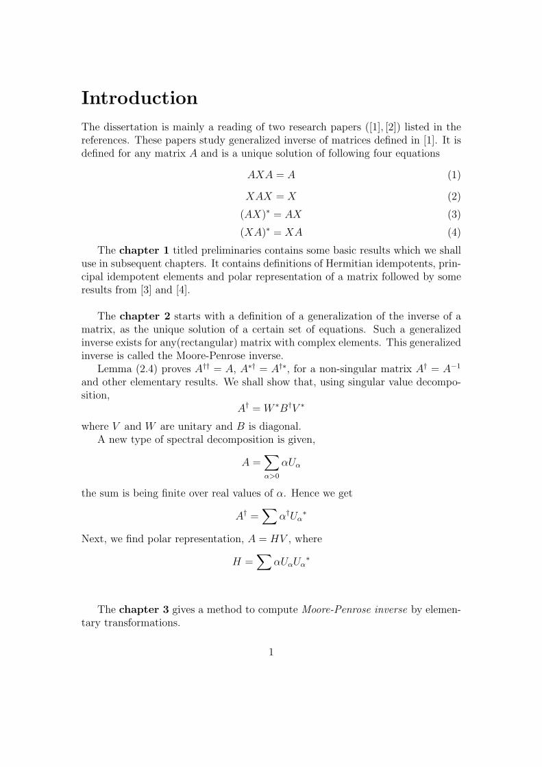
Introduction

The dissertation is mainly a reading of two research papers ([1], [2]) listed in thereferences. These papers study generalized inverse of matrices defined in [1]. It isdefined for any matrix A and is a unique solution of following four equations

AXA = A (1)

XAX = X (2)

(AX)∗ = AX (3)

(XA)∗ = XA (4)

The chapter 1 titled preliminaries contains some basic results which we shalluse in subsequent chapters. It contains definitions of Hermitian idempotents, prin-cipal idempotent elements and polar representation of a matrix followed by someresults from [3] and [4].

The chapter 2 starts with a definition of a generalization of the inverse of amatrix, as the unique solution of a certain set of equations. Such a generalizedinverse exists for any(rectangular) matrix with complex elements. This generalizedinverse is called the Moore-Penrose inverse.

Lemma (2.4) proves A†† = A, A∗† = A†∗, for a non-singular matrix A† = A−1

and other elementary results. We shall show that, using singular value decompo-sition,

A† = W ∗B†V ∗

where V and W are unitary and B is diagonal.A new type of spectral decomposition is given,

A =∑α>0

αUα

the sum is being finite over real values of α. Hence we get

A† =∑

α†Uα∗

Next, we find polar representation, A = HV , where

H =∑

αUαUα∗

The chapter 3 gives a method to compute Moore-Penrose inverse by elemen-tary transformations.

1

Chapter 1

Preliminaries

Recall that the conjugate transpose A∗ = (A)T of a matrix A has following prop-erties

A∗∗ = A

(A+B)∗ = A∗ +B∗

(λA)∗ = λA∗

(BA)∗ = A∗B∗

AA∗ = 0 ⇒ A = 0

Since,

Trace(AA∗) =n∑

i=1

⟨ai.a∗i ⟩ =n∑

i=1

⟨ai, ai

⟩=

n∑i=1

n∑j=1

|aij|2

i.e., the trace of AA∗ is the sum of the squares of the moduli of the elements of A.Hence the last property.Observe that using fourth and fifth property we can obtain the rule

BAA∗ = CAA∗ ⇒ BA = CA (1.1)

Since,

(BAA∗ − CAA∗)(B − C)∗ = (BAA∗ − CAA∗)(B∗ − C∗)

= BAA∗B∗ − CAA∗B∗ −BAA∗C∗ + CAA∗C∗

= (BA− CA)A∗B∗ − (BA− CA)A∗C∗

= (BA− CA)(A∗B∗ − A∗C∗)

= (BA− CA)(BA− CA)∗

2

Similarly,

(BA∗A− CA∗A)(B − C)∗ = (BA∗ − CA∗)(BA∗ − CA∗)∗

and henceBA∗A = CA∗A⇒ BA∗ = CA∗ (1.2)

Definition 1.1. Hermitian Idempotents: A Hermitian idempotent matrix isone satisfying EE∗ = E, that is,

E = E∗ and E2 = E.

Note 1.2. If E = E∗ and E2 = E then

E2 = E ⇒ EE = E ⇒ EE∗ = E

If EE∗ = E thenEE∗ = E

⇒ EE∗ = E∗

⇒ E = E∗

⇒ EE∗ = E2 = E

Definition 1.3. Principal idempotent elements of a matrix: For anysquare matrix A there exists a unique set of matrices Kλ defined for each com-plex number λ such that

KλKµ = δλµKλ (1.3)∑Kλ = I (1.4)

AKλ = KλA (1.5)

(A− λI)Kλ is nilpotent (1.6)

the non-zero K ′λs are called principal idempotent elements of a matrix.

Remark 1.4. Existence of K ′λs: Let ϕ (x) = (x− λ1)

n1 . . . (x− λr)nr be the

minimal polynomial of A where the factors (x− λi)ni are mutually coprime i.e.,

there exists fi (x), fj (x) such that

fi (x) (x− λi)ni + fj (x) (x− λj)

nj = 1 ; i ̸= j

We can write ϕ (x) = (x− λi)ni ψi (x) where

ψi (x) =r∏

j=1 j ̸=i

(x− λj)nj

3

As ψ′is are co-prime, there exist polynomials χi (x) such that∑

χi (x)ψi (x) = 1

putKλi

= χi (x)ψi (x)

with the other K ′λs zero. So that

∑Kλ = I. Further,

(A− λiI)Kλi= (A− λiI)χi (x)ψi (x)

⇒ [(A− λiI)Kλi]ni = 0

If λ is not an eigen value of A, Kλ is zero so that sum in equation (1.4) is finite.Further note that,

KλKµ = 0 if λ ̸= µ

and as the sum∑Kλ is finite,

Kλ2 = Kλ.

Hence,KλKµ = δλµKλ.

It is clear thatAKλ = KλA.

Theorem 1.5. Polar representation of a matrix: Any square matrix is theproduct of a Hermitian with an unitary matrix.

Theorem 1.6. [[3], 3.5.6] :The following are equivalent

1. r(AB)=r(B).

2. Row space of AB is same as row space of B.

3. B=DAB for some matrix D

Theorem 1.7. Rank Cancellation laws [[3], 3.5.7] :

1. If ABC=ABD and r(AB)=r(B) then BC=BD.

2. If CAB=DAB and r(AB)=r(A) then CA=DA.

Definition 1.8. Rank factorization: Let A be an m×n matrix with rank r ≥ 1,then (P,Q) is said to be a rank factorization of A if Pm×r, Qr×n and A = PQ.

Theorem 1.9. If any matrix A is idempotent then it’s rank and trace are equal.

4

Proof. Let r ≥ 1 be the rank of A and (P,Q) be a rank factorization of A. Thensince A is idempotent i.e,

A2 = A

⇒ PQPQ = PQ = PIrQ

Since P can be cancelled on the left and Q can be cancelled on right (since we canwrite PIrQPQ = PIrQ), we get

QP = Ir

Now,trace(Ir) = r

andtrace(PQ) = trace(QP ) = r

Hence, the rank is equal to the trace.

Theorem 1.10. [[3], 8.7.8] : A matrix is unitarily similar to a digonal matrix ifand only if it is normal.

Theorem 1.11. [[4], chapter 8, theorem 18] : Let V be a finite dimensional innerproduct space, and let T be a self-adjoint linear operator on V . Then there is anorthonormal basis for V , each vector of which is a characterstic vector for T .

Corollary 1.12. [[4], chapter 8, corollary to theorem 18] : Let A be an n× n Her-mitian (self-adjoint) matrix. Then there is a unitary matrix P such that P−1APis diagonal, that is, A is unitarily equivalent to diagonal matrix.

Note 1.13. If two matrices A and B are Hermitian and having same eigen valuesthen they are equivalent under a unitary transformation.

Theorem 1.14. [[4], chapter 9, theorem 13] : Let V be a finite dimensional innerproduct space and T is a non-negative operator on V . Then T has a unique non-negative square root that is, there is one and only one non-negative operator N onV such that N2 = T .

Theorem 1.15. [[4], chapter 9, theorem 14] : Let V be a finite dimensional innerproduct space and let T be any linear operator on V . Then there exists a unitaryoperator U on V and a non-negative operator N on V such that T = UN . Thenon-negative operator N is unique. If T is invertible, the operator U is also unique.

Remark 1.16. If any matrix T is non-singular then it’s polar representation isunique.

5

Chapter 2

A generalized inverse for matrices

Following theorem gives the generalized inverse of a matrix. It is the uniquesolution of a certain set of equations

Theorem 2.1. The four equations

AXA = A, (2.1)

XAX = X (2.2)

(AX)∗ = AX (2.3)

(XA)∗ = XA (2.4)

have a unique solution for any matrix A.

Proof. First, we observe that the equations (2.2) and (2.3) are equivalent to thesingle equation

XX∗A∗ = X (2.5)

substitute equation (2.3) in (2.2) to get

X (AX)∗ = X

XX∗A∗ = X

Conversely, suppose equation (2.5) holds. We have

AXX∗A∗ = AX

⇒ AX (AX)∗ = AX

Obeserve that AXX∗A∗ is Hermitian, Thus (AX)∗ = AX. If we put (2.3) in (2.5),we get equation (2.2).Similarly, equations (2.1) and (2.4) are equivalent to the single equation

XAA∗ = A∗ (2.6)

6

Since, (2.1) and (2.4) gives

AXA = A

⇒ A (XA)∗ = A

⇒ (A (XA)∗)∗

= XAA∗ = A∗

Futher, if XAA∗ = A∗ then

(XAA∗)∗ = AA∗X∗ = A

⇒ XAA∗X∗ = XA

⇒ (XA)∗ = XA (since XAA∗X∗ is Hermitian)

Next, if we substitute (2.4) in (2.6), we get (2.1).Thus it is sufficient to find an X satisfying (2.5) and (2.6), such X will exists

if a B can be found satisfying

BA∗AA∗ = A∗

Then X = BA∗ satisfies (2.6). Observe that, from equation (2.6),

XAA∗ = A∗

⇒ (XA)∗A∗ = A∗ (from(2.4))

⇒ A∗X∗A∗ = A∗

⇒ BA∗X∗A∗ = BA∗

⇒ XX∗A∗ = X

i.e., X also satisfies (2.5).As a matrix satisfies its characteristic equation, the expressionsA∗A, (A∗A)2, . . .

cannot be linearly independent i.e., there are λ′is; i = 1, 2, . . . , k such that

λ1A∗A+ λ2(A

∗A)2 + · · ·+ λk(A∗A)k = 0 (2.7)

where λ1, λ2, . . . , λk are not all zero. Note that k need not be unique. Let λr bethe first non-zero λ then (2.7) becomes

λr (A∗A)r + λr+1 (A

∗A)r+1 + · · ·+ λk (A∗A)k = 0

7

⇒ (A∗A)r = −λ−1r

[λr+1 (A

∗A)r+1 + · · ·+ λk (A∗A)k

]= −λ−1

r

[λr+1I + λr+2A

∗A+ · · ·+ λk (A∗A)k−r−1

](A∗A)r+1

If we put

B = −λ−1r

[λr+1I + λr+2A

∗A+ · · ·+ λk (A∗A)k−r−1

]then

B (A∗A)r+1 = (A∗A)r

We can write this equation as

B (A∗A)r (A∗A) = (A∗A)r−1 (A∗A)

⇒ B (A∗A)r A∗ = (A∗A)r−1A∗ (by (1.2))

⇒ B (A∗A)r = (A∗A)r−1 (by (1.1))

Thus, by repeated applications of (1.2) and (1.1), we get

B (A∗A)2 = A∗A

⇒ BA∗AA∗ = A∗ again (by (1.2)),

This is what was required. Now, to show that this X is unique. Let there be Xand Y which satisfy (2.5) and (2.6).If we substitute (2.4) in (2.2) and (2.3) in (2.1), we get

Y = A∗Y ∗Y (2.8)

A∗ = A∗AY (2.9)

Now

X = XX∗A∗ (2.5)

= XX∗A∗AY (by (2.9))

= XAY [since AXA = A⇒ (AX)∗A = A⇒ X∗A∗A = A]

= XAA∗Y ∗Y (by (2.8))

= A∗Y ∗Y (by (2.6))

= Y (by (2.8))

8

Thus the solution of (2.1), (2.2), (2.3), (2.4) is unique.Conversely, if A∗X∗X = X then

A∗X∗XA = XA

and LHS is Hermition, so, (XA)∗ = XA. Now, if we substitute (XA)∗ = XA inA∗X∗X = X, we get

XAX = X

which is (2.2). Thus, (2.4) and (2.2) are equivalent to (2.8). Similarly, (2.3) and(2.1) are equivalent to (2.9).

Definition 2.2. Generalized inverse: The unique solution of

AXA = A,

XAX = X,

(AX)∗ = AX,

(XA)∗ = XA

is called the gerneralized inverse of A. We write X = A†.

Note 2.3. To calculateA†, we only need to solve the two unilateral linear equations

XAA∗ = A∗ (2.10)

andA∗AY = A∗ (2.11)

Put A† = XAY . Note that XA and AY are Hermitian and satisfy

AXA = A = AY A (Use cancellation laws)

Then,

1. AA†A = AXAY A = AY A = A

2. A†AA† = XAY AXAY = XAXAY = XAY = A†

3. (AA†)∗ = (AXAY )∗ = (AY )∗ = AY = AXAY = AA† (since AY is Hermi-tian)

4. (A†A)∗ = (XAY A)∗ = (XA)∗ = XA = XAY A = A†A (since AX is Hermi-tian)

9

Thus, if X and Y are solutions of unilateral linear equations (2.10) and (2.11) thenXAY is the generalized inverse.Moreover, (2.5) and (2.6) are also satisfied i.e.,

A†A†∗A∗ = A† (2.12)

A†AA∗ = A∗ (2.13)

and (2.8) and (2.9) are,A∗A†∗A† = A† (2.14)

A∗AA† = A∗ (2.15)

Lemma 2.4.

2.4.1 A†† = A.2.4.2 A∗† = A†∗.2.4.3 If A is non-singular A† = A−1.2.4.4 (λA)† = λ†A†.2.4.5 (A∗A)† = A†A†∗.2.4.6 If U and V are unitary, (UAV )† = V ∗A†U∗.2.4.7 If A =

∑Ai, where AiA

∗j = 0 and

A∗iAj = 0 whenever i ̸= j then A† =

∑A†

i .2.4.8 If A is normal A†A = AA† and (An)† = (A†)n.2.4.9 A, A∗A, A† and A†A all have rank equal to trace of A†A.

Proof. 2.4.1. To show that A is the generalized inverse of A† i.e., to show that

A†AA† = A†

AA†A = A(A†A

)∗= A†A(

AA†)∗ = AA†

which are (2.2), (2.1), (2.4), (2.3). Hence

A†† = A.

2.4.2. To show that the generalized inverse of A∗ is A†∗ i.e., to show that (2.1),(2.2), (2.3), (2.4) holds when X is replaced by A†∗ and A by A∗

A∗A†∗A∗ = (AA†A)∗ = A∗ (by (2.1))

A†∗A∗A†∗ = (A†AA†)∗ = A†∗ (by (2.2))

10

(A∗A†∗)∗ = (A†A)∗∗ = A†A (since A∗∗ = A)

= (A†A)∗ (by equation (2.3))

= A∗A†∗

(A†∗A∗)∗ = (AA†)∗∗ = AA† (by equation (2.4))

= A†∗A∗

2.4.3. Observe

AA−1A = A

A−1AA−1 = A−1(AA−1

)∗= I∗ = I = AA−1(

A−1A)∗

= I∗ = I = A−1A

2.4.4. To show that λ†A† is the generalized inverse of λA.

(λA)(λ†A†) (λA) = λA

1

λA†λA = λAA†A = λA (by(2.1))

(λA)† (λA) (λA)† =(λ†A†) (λA)

(λ†A†) = 1

λA†λAλ†A† = λ†A†AA† = λ†A† (by(2.2))

((λA)

(λ†A†))∗ = (λA1

λA†)∗

=(AA†)∗ = AA† = λA

1

λA† = (λA)

(λ†A†) (by(2.3))

(λ†A†λA

)∗=

(1

λA†λA

)∗

=(A†A

)∗= A†A =

1

λA†λA =

(λ†A†) (λA) (by(2.4))

2.4.5. To show that A†A†∗ is the generalized inverse of A∗A.

(A∗A)(A†A†∗) (A∗A) = A∗AA† (AA†)∗A

= A∗AA†AA†A

= A∗AA†A (by (2.2))

= A∗A (by (2.1))(A†A†∗) (A∗A)

(A†A†∗) = A†AA†A†∗

= A†A†∗ (by (2.2))

11

(A†A†∗)∗ (A∗A)∗ = A†A†∗A∗A

= A†A (by (2.12))

=(A†A

)∗(by (2.4))

= A∗A†∗

= A∗AA†A†∗ (by (2.15))

= (A∗A)(A†A†∗)

(A∗A)∗(A†A†∗)∗ = A∗AA†A†∗

=((A∗A)

(A†A†∗))∗ (since (2.3) holds for A∗A)

=(A†A†∗)∗ (A∗A)∗

=(A†A†∗) (A∗A)

2.4.6. To show that V ∗A†U∗ is the generalized inverse of UAV .Note that since U and V are unitary, UU∗ = U∗U = I, V V ∗ = V ∗V = I. Then

(UAV )(V ∗A†U∗) (UAV ) = UAA†AV = UAV (by (2.1))(

V ∗A†U∗) (UAV )(V ∗A†U∗) = V ∗A†AA†U∗ = V ∗A†U∗ (by (2.2))(

V ∗A†U∗)∗ (UAV )∗ =(UA†∗V

)(V ∗A∗U∗)

= UA†∗A∗U∗

= U(AA†)∗ U∗

= UAA†U∗ (by (2.3))

= (UAV )(V ∗A†U∗) (since V V ∗ = I)

12

(UAV )∗(V ∗A†U∗)∗ = (V ∗A∗U∗)

(UA†∗V

)= V ∗A∗A†∗V

= V ∗ (A†A)∗V

= V ∗A†AV (by (2.4))

=(V ∗A†U∗) (UAV ) (since U∗U = I)

2.4.7. To show that∑A+

i is the generalized inverse of (∑Ai). First observe that,

sinceA†

j = A∗j A

†∗j A†

j, (2.14)

⇒ AiA†j = AiA

∗jA

†∗j A

†j

⇒ AiA†j = 0,whenever i ̸= j

since AiA∗j = 0, whenever i ̸= j.

Also as,A†

i = A†i A

†∗i A∗

i , (2.12)

⇒ A†iAj = 0,whenever i ̸= j

since A∗iAj = 0, whenever i ̸= j.

Now,

(∑

iAi)(∑

j A†j

)(∑

k Ak) = (∑

iAi)(∑

j A†jAj

)=∑

i

(AiA

†iAi

)=∑

iAi

Similarly, as above (∑A†

i

) (∑Ai

) (∑A†

i

)=(∑

A†i

)

13

Then, ((∑

iAi)(∑

j A†j

))∗=(∑

j A†∗j

)(∑

iA∗i )

=∑

iA†∗i A∗

i

=∑

i

(AiA

†i

)∗=∑

iAiA†i

= (∑

iAi)(∑

iA†i

) [since AiA

†j = 0

]Similarly, as above (∑

i

A†i

∑j

Aj

)∗

=∑i

A†i

∑j

Aj

2.4.8. Since AA∗ is Hermitian and as we have proved in (2.4.5). that (A∗A)† =A†A†∗, similarly we can show that (AA∗)† = A†∗A†. By using this fact we see that

A†A = A†A†∗A∗A

= (A∗A)† (A∗A) (by 2.4.5)

= (AA∗)† (AA∗) (since A is normal)

= A†∗A†AA∗

= A†∗A∗ (using (2.13))

=(AA†)∗ = AA† (

since(AA†)∗ = AA†)

Now, to show that(A†)n is generlized inverse of An. As AA† = A†A

(An)(A†)n (An) =

(AA†A

)n= An(

A†)n (A)n(A†)n =

(A†AA†)n =

(A†)n(

An(A†)n)∗ =

(AA†)∗n =

((AA†)∗)n =

(AA†)n = An

(A†)n

((A†)nAn

)∗=(A†A

)∗n=((A†A

)∗)n=(A†A

)n=(A†)nAn

14

So,(An)† = (A†)n

2.4.9. First note that(A†A)2 = A†AA†A = A†A

i.e., A†A is an idempotent. By theorem (1.9), it’s rank is trace of it.

Remark 2.5. Since by equation (2.12), we can write

A† = A†A†∗A∗ = (A∗A)†A∗ (by (2.4.5)) (2.16)

so we can calculate the generalized inverse of a matrix A from the generalizedinverse of A∗A. As A∗A is Hermitian it can be reduced to diagonal form by aunitary transformation i.e.,

A∗A = UDU∗

where U is unitary and D = diag (α1, α2, ....., αn). Then

D† = diag(α†1, α

†2, ....., α

†n

)By (2.4.6) we can write,

(A∗A)† = UD†U∗

⇒ A† = UD†U∗A∗ (by (2.16))

Note 2.6. By singular value decomposition, we know that any square matrix Acan be written in the form A = V BW where V and W are unitary and B isdiagonal. Also since AA∗ and A∗A are both Hermitian and have the same eignvalues, there exists a unitary matrix T such that TAA∗T ∗ = A∗A (by (1.13)),observe that,

(TA) (TA)∗ = TAA∗T ∗ = A∗A(TA)∗ (TA) = A∗T ∗TA = A∗A (since T ∗T = I)

i.e., TA is normal and so diagonable by unitary transformation (from (1.10)).As above by (2.4.6) we get

A† = W ∗B†V ∗

Remark 2.7. Observe that

† :Mm×n(IR) →Mn×m(IR)

A 7−→ †(A) = A†

15

Now, consider

Aϵ =

(1 00 ϵ

)⇒ A−1

ϵ =

(1 00 ϵ−1

)We have

limϵ→0

Aϵ =

(1 00 0

),

which is a singular matrix but Aϵ is a non-singular. Thus, in this case

Aϵ → A but † (Aϵ) ̸→ †(A) =(

1 00 0

).

But if rank of A is kept fixed then the function † is continuous.

Theorem 2.8. A necessary and sufficient condition for the equation AXB = Cto have a solution is

AA†CB†B = C

in which case the general solution is

X = A†CB† + Y − A†AY BB†

where Y is arbitrary.

Proof. Suppose X satisfies AXB = C. Then

C = AXB = AA†AXBB†B = AA†CB†B

Conversely, if C = AA†CB†B, then X = A†CB† is a particular solution of C =AXB.

For general solution we will have to solve AXB = 0. For

X = Y − A†AY BB†,

where Y is arbitrary, we have,

AXB = AY B − AA†AY BB†B = 0

since AA†A = A, BB†B = B.

Corollary 2.9. The general solution of the vector equation Px = c is

x = P †c+(I − P †P

)y

where y is arbitrary provided that the equation has a solution.

16

Proof. By the above theorem,

x = P †cI + y − P †PyII†

= P †c+ y − P †Py

= P †c+(I − P †P

)y

where y is arbitrary.

Corollary 2.10. A necessary and sufficient condition for the equations AX =C, XB = D to have a common solution is that each equation should individuallyhave a solution and that AD = CB.

Proof. The condition is obviously necessary since,

AX = C⇒ AXB = CB⇒ AD = CB (since XB = D)

Now, to show the condition is sufficient. Put

X = A†C +DB† − A†ADB†

ThenAX = A

(A†C +DB† − A†ADB†)

= AA†C + ADB† − AA†ADB†

= AA†C + ADB† − ADB†

= AA†C

andXB =

(A†C +DB† − A†ADB†)B

= A†CB +DB†B − A†ADB†B

= A†CB +DB†B − A†CB (since AD = CB)

= DB†B

So X = A†C + DB† − A†ADB† will be a solution if the condition AA†C = C,DB†B = D and AD = CB are satisfied.

17

Lemma 2.11.

2.11.1. A†A,AA†, I − A†A, I − AA† are all Hermitian idempotents.2.11.2. If E is Hermitian idempotent, E† = E.2.11.3. K is idempotent if and only if there exist Hermitian idempotents Eand F

such that K = (FE)† in which case K = EKF.

Proof. 2.11.1. First to show that(A†A

) (A†A

)∗= A†A.(

A†A) (

A†A)∗

= A†AA∗A†∗ = A∗A†∗ (by (2.13))

=(A†A

)∗= A†A

(since A†A is Hermitian

)Similarly, (

AA†) (AA†)∗ = AA†A†∗A∗

= AA† (by (2.12))

Now,(I − A†A

) (I − A†A

)∗=(I − A†A

) (I − A∗A†∗)

= I − A∗A†∗ − A†A+ A†AA∗A†∗

= I − A∗A†∗ − A†A+ A∗A†∗ (by (2.13))

= I − A†A

and,(I − AA†) (I − AA†)∗ =

(I − AA†) (I − A†∗A∗)

= I − A†∗A∗ − AA† + AA†A†∗A∗

= I − A†∗A∗ − AA† + AA† (by (2.12))

= I −(AA†)∗

= I − AA† (since AA† is Hermitian

)2.11.2. Suppose E = E∗ and E2 = E. Then

EEE = E

18

and(EE)∗ = E∗E∗ = EE

Therefore, (2.1), (2.2), (2.3) and (2.4) hold.

2.11.3. First let K be idempotent i.e., K2 = K. As,

K† = K†KK†

⇒ K† = K†K.KK†

⇒ K†† =((K†K

) (KK†))†

⇒ K = (FE)†(since K†† = K

)where F = K†K and E = KK†. Clearly F and E are Hermitian idempotents.Further,

EKF = KK†KK†K

= KK†K

= K

Conversely, if K = (FE)† then

K2 = (EKF )2 = EKFEKF (since K = EKF )

= E (FE)† (FE) (FE)† F(put K = (FE)†

)= E (FE)† F

(since A†AA† = A

)= EKF

= K

so K is idempotent.

Theorem 2.12. IfEλ = I − {(A− λI)n}† (A− λI)n

andFλ = I − (A− λI)n {(A− λI)n}† ,

19

where n is sufficientely large (e.g. the order of A), then the principal idempotentelements of A are given by Kλ = (FλEλ)

†. Further, n can be taken as unity if andonly if A is diagonalizable.

Proof. First suppose that A is diagonalizable. Put

Eλ = I − (A− λI)† (A− λI)

andFλ = I − (A− λI) (A− λI)†

By (2.11.1) Eλ and Fλ are Hermitian idempotents. If λ is not an eigen value of A,then for no non-zero x,

(A− λI) x ̸= 0

⇒ Ker (A− λI) = 0

⇒ A− λI is invertible

⇒ (A− λI)† = (A− λI)−1 (by (2.4.3))

⇒ (A− λI)† (A− λI) = I

⇒ Eλ = Fλ = 0

Now,

(A− µI)Eµ = (A− µI)[I − (A− µI)† (A− µI)

]= (A− µI)− (A− µI) (A− µI)† (A− µI)

= (A− µI)− (A− µI)

= 0

(A− µI)Eµ = 0 (2.17)

Similarly,Fλ (A− λI) = 0 (2.18)

So that,

(A− µI)Eµ = 0 ⇒ AEµ = µEµ

20

⇒ FλAEµ = µFλEµ (2.19)

Fλ (A− µI) = 0 ⇒ FλA = λFλ

⇒ FλAEµ = λFλEµ (2.20)

(2.19) and (2.20) imply

λFλEµ = FλAEµ = µFλEµ

⇒ (λ− µ)FλEµ = 0

⇒ FλEµ = 0 if λ ̸= µ (2.21)

By (2.11.3) we have Kλ = (FλEλ)† and

Kλ = EλKλFλ = Eλ (FλEλ)† Fλ (2.22)

So,λ = µ⇒ KλKµ = Eλ (FλEλ)

† (FλEλ) (FλEλ)† Fλ

= Eλ (FλEλ)† Fλ

= Kλ

and if λ ̸= µ,KλKµ = 0, since FλEµ = 0. Hence

KλKµ = δλµKλ (2.23)

also equation (2.21) gives

FλKµEν = δλµδµνFλEλ (2.24)

Next, Zα be any eigen vector ofA corresponding to the eigen value α. (i.e., (A− αI)Zα = 0).Then

EαZα =(I − (A− αI)† (A− αI)

)Zα

= Zα − (A− αI)† (A− αI)Zα

= Zα

Since A is diagonalizable, any column vector x conformable with A is expressibleas a finite sum over all complex λ. i.e.,

x =∑

Zλ =∑

Eλxλ

21

Similarly, if y∗ is conformable with A, it is expressible as

y∗ =∑

y∗λFλ

Now

y∗ (∑Kµ)x = (

∑y∗λFλ) (

∑Kµ) (

∑Eνxν)

=∑y∗λFλEλxλ (by (2.23) and (2.24))

= (∑y∗λFλ) (

∑Eνxν)

= y∗x

Hence, ∑Kµ = I (2.25)

Also from equation (2.17) we have

(A− λI)Eλ = 0

⇒ AEλ = λEλ

⇒ AEλ (FλEλ)† Fλ = λEλ (FλEλ)

† Fλ

⇒ AKλ = λKλ (by (2.22)) (2.26)

AlsoFλ (A− λI) = 0

⇒ FλA = λFλ

⇒ Eλ (FλEλ)† FλA = λEλ (FλEλ)

† Fλ

⇒ KλA = λKλ (by (2.22)) (2.27)

From (2.26) and (2.27) we have

AKλ = λKλ = KλA (2.28)

Thus conditions (1.5) and (1.6) are satisfied. Now, as∑Kλ = I,

A =∑

λKλ (2.29)

Conversely, let n = 1 and suppose A is not diagonalizable.Observe that, by (2.28)

AKλx = λKλx

22

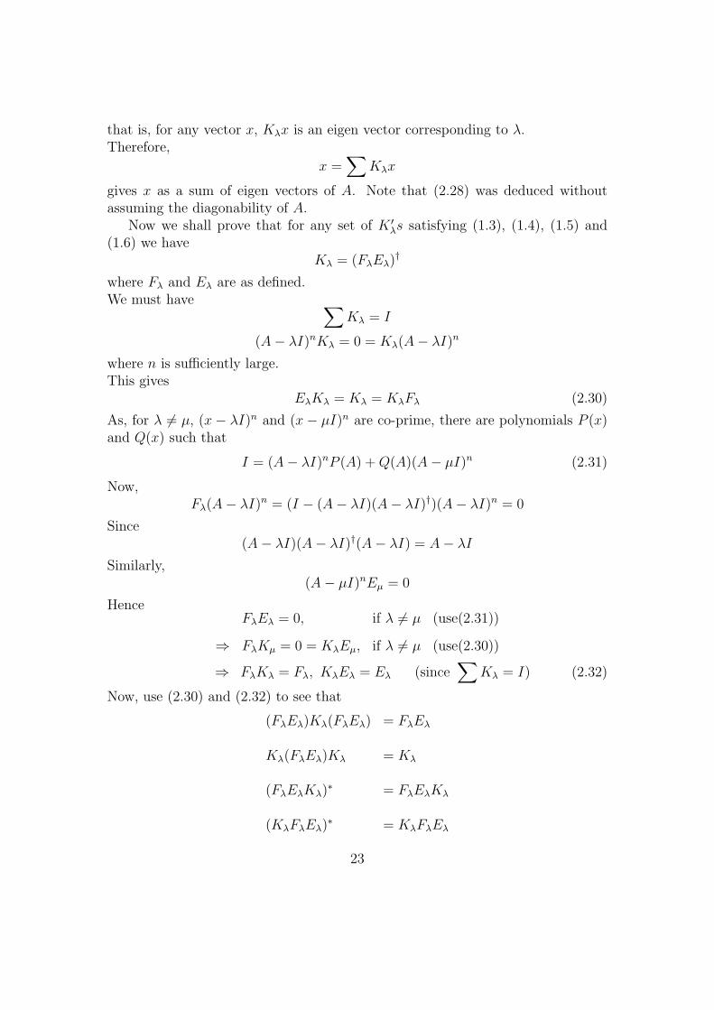
that is, for any vector x, Kλx is an eigen vector corresponding to λ.Therefore,

x =∑

Kλx

gives x as a sum of eigen vectors of A. Note that (2.28) was deduced withoutassuming the diagonability of A.

Now we shall prove that for any set of K ′λs satisfying (1.3), (1.4), (1.5) and

(1.6) we haveKλ = (FλEλ)

†

where Fλ and Eλ are as defined.We must have ∑

Kλ = I

(A− λI)nKλ = 0 = Kλ(A− λI)n

where n is sufficiently large.This gives

EλKλ = Kλ = KλFλ (2.30)

As, for λ ̸= µ, (x− λI)n and (x− µI)n are co-prime, there are polynomials P (x)and Q(x) such that

I = (A− λI)nP (A) +Q(A)(A− µI)n (2.31)

Now,Fλ(A− λI)n = (I − (A− λI)(A− λI)†)(A− λI)n = 0

Since(A− λI)(A− λI)†(A− λI) = A− λI

Similarly,(A− µI)nEµ = 0

HenceFλEλ = 0, if λ ̸= µ (use(2.31))

⇒ FλKµ = 0 = KλEµ, if λ ̸= µ (use(2.30))

⇒ FλKλ = Fλ, KλEλ = Eλ (since∑

Kλ = I) (2.32)

Now, use (2.30) and (2.32) to see that

(FλEλ)Kλ(FλEλ) = FλEλ

Kλ(FλEλ)Kλ = Kλ

(FλEλKλ)∗ = FλEλKλ

(KλFλEλ)∗ = KλFλEλ

23

These equations can be verified as below:

(FλEλ)Kλ(FλEλ) = FλEλKλFλEλ

= FλKλFλEλ (by(2.30))= FλKλEλ (by(2.30))= FλEλ (by(2.32))

Kλ(FλEλ)Kλ = KλFλEλKλ

= KλFλKλ (by(2.30))= KλFλ (by(2.32))= Kλ (by(2.30))

(FλEλKλ)∗ = (FλKλ)

∗ (by(2.30))= Fλ

∗ (by(2.32))= Fλ (since Fλ is Hermitian idempotent)= FλKλ (by(2.32))= FλEλKλ (by(2.30))

(KλFλEλ)∗ = (KλEλ)

∗ (by(2.30))= Eλ

∗ (by(2.32))= Eλ (since Eλ is Hermitian idempotent)= KλEλ (by(2.32))= KλFλEλ (by(2.30))

Hence,(FλEλ)

† = Kλ

and Kλ is unique.

Corollary 2.13. If A is normal, it is diagonalizable and its principal idempotentelements are Hermitian.

Proof. If A is normal then (A− λI) is also normal. Then by (2.4.8)

(A− λI)(A− λI)† = (A− λI)†(A− λI)

Then

Eλ = I − (A− λI)†(A− λI) = Fλ

and Kλ = (FλEλ)† is Hermitian since Eλ and Fλ both are Hermitian.

24

Note 2.14. If A is normal then

A† = (∑λEλ)

† (since A =∑λEλ)

=∑

(λEλ)† (by (2.4.7))

=∑λ†Eλ

† (by (2.4.4))

=∑λ†Eλ

(since Eλ is Hermitian so E† = E

)A new type of Spectral Decomposition: In view of above note it is

clear that if A is normal then we get a simple expression for A† in terms of itsprincipal idempotent elements. However, below, we prove a new type of spectraldecomposition so that we get relatively simple expression for A†.

Theorem 2.15. Any matrix A is uniquely expressible in the form

A =∑α>0

αUα

this being a finite sum over real values of α, where

U †α = U∗

α (2.33)

U∗αUβ = 0 (2.34)

UαU∗β = 0 (2.35)

if α ̸= β.Thus using above note we can write

A† =∑

α†U∗α [since U †

α = U∗α]

Proof. Equations (2.33), (2.34) and (2.35) can be comprehensively written as

UαU∗βUγ = δαβδβγUα (2.36)

For α = β = γ

UαU∗αUα = Uα

⇒ U∗αUαU

∗α = U∗

α

Also, note that UαU∗α and U∗

αUα are both Hermitian. Therefore, by uniqueness ofgeneralized inverse

U †α = U∗

α (2.37)

25

Also,UαU

∗αUβ = 0 and UαU

∗βUβ = 0

respectively imply

U∗αUβ = 0 and UαU

∗β = 0 (by (1.2))

DefineEλ = I − (A∗A− λI)†(A∗A− λI)

The matrix A∗A is normal, being Hermitian and is non-negative definite. Hencethe non-zero Eλ’s are it’s principal idempotent elements. (by corollary 2.13) andEλ = 0 unless λ ≥ 0. Thus

A∗A =∑

λEλ

and(A∗A)† =

∑λ†Eλ

HenceA†A = A†A†∗A∗A = (A∗A)†A∗A =

∑λ†λEλ =

∑λ>0

Eλ

Put

Uα =

{α−1AEα2 if α > 00 otherwise

Then ∑αUα =

∑α>0

αα−1AEα2 = A∑λ>0

Eλ = AA†A = A

Also, if α, β, γ > 0 then

UαU∗βUγ = (α−1AEα2)(β−1AEβ2)∗(γ−1AEγ2)

= α−1β−1γ−1AEα2E∗β2A∗AEγ2

= α−1β−1γ−1AEα2Eβ2(∑λ†Eλ)Eγ2 (E∗

α = Eα)

= α−1β−1γ−1AEα2Eβ2(γ2Eγ2) (EλEµ = δλµEλ)

= δαβδβγα−1AEα2

= δαβδβγUα

For uniqueness suppose

A =∑α>0

αVα where VαV∗β Vγ = δαβδβγVα

26

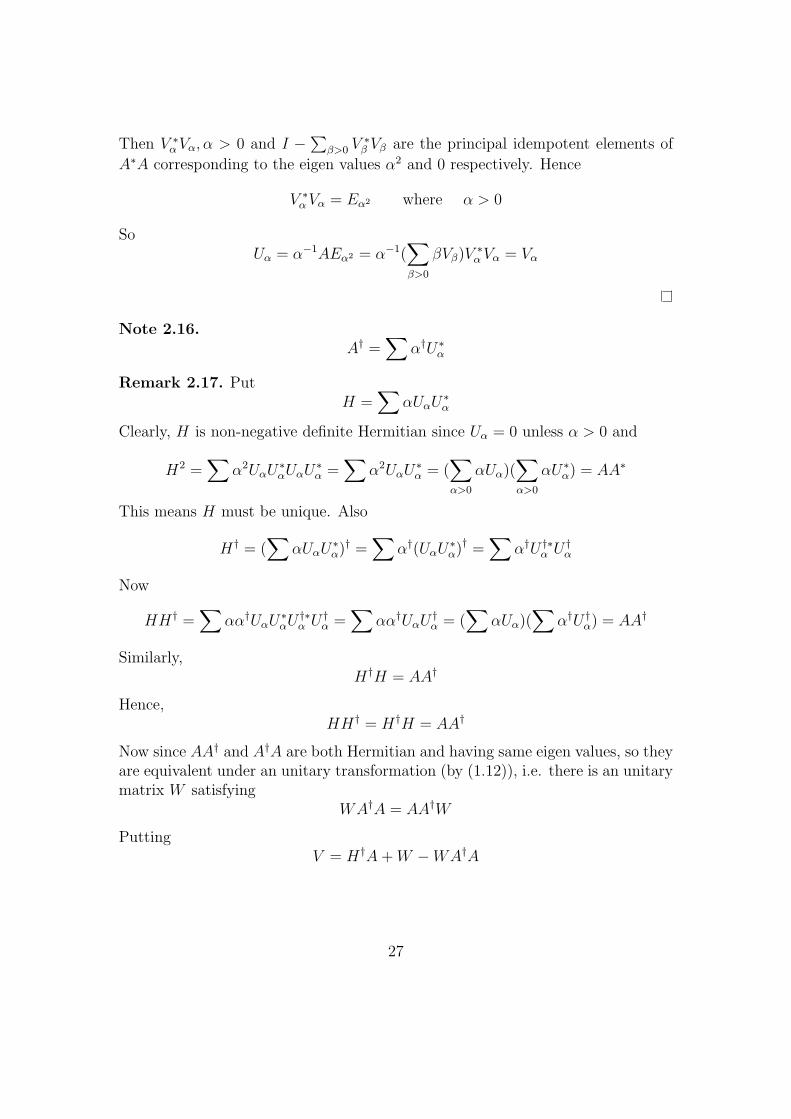
Then V ∗αVα, α > 0 and I −

∑β>0 V

∗β Vβ are the principal idempotent elements of

A∗A corresponding to the eigen values α2 and 0 respectively. Hence

V ∗αVα = Eα2 where α > 0

SoUα = α−1AEα2 = α−1(

∑β>0

βVβ)V∗αVα = Vα

Note 2.16.A† =

∑α†U∗

α

Remark 2.17. PutH =

∑αUαU

∗α

Clearly, H is non-negative definite Hermitian since Uα = 0 unless α > 0 and

H2 =∑

α2UαU∗αUαU

∗α =

∑α2UαU

∗α = (

∑α>0

αUα)(∑α>0

αU∗α) = AA∗

This means H must be unique. Also

H† = (∑

αUαU∗α)

† =∑

α†(UαU∗α)

† =∑

α†U †∗α U

†α

Now

HH† =∑

αα†UαU∗αU

†∗α U

†α =

∑αα†UαU

†α = (

∑αUα)(

∑α†U †

α) = AA†

Similarly,H†H = AA†

Hence,HH† = H†H = AA†

Now since AA† and A†A are both Hermitian and having same eigen values, so theyare equivalent under an unitary transformation (by (1.12)), i.e. there is an unitarymatrix W satisfying

WA†A = AA†W

PuttingV = H†A+W −WA†A

27

we get

V V ∗ = (H†A+W −WA†A)(A∗H∗† +W ∗ − A∗A∗†W ∗)

= H†AA∗H∗† +WA∗H∗† −WA†AA∗H∗†

+H†AW ∗ +WW ∗ −WA†AW ∗

−H†AA∗A∗†W ∗ −WA∗A∗A∗†W ∗ +WA†AA∗A∗†W ∗

= H†AA∗H∗† +WA∗H∗† −WA∗H∗†

+H†AW ∗ + I − AA†WW ∗ (since WA†A = AA†W )

−H†AW ∗ −WA∗A∗†W ∗ +WA∗A∗†W ∗ (since A∗ = A†AA∗ and WW ∗ = I)

= H†AA∗H∗† + I − AA†

= H†H2H∗† + I − AA† (since H2 = AA∗)

= AA†HH∗† + I − AA†

= AA†HH† + I − AA† (since H is nnd Hermitian H = H∗)

= (AA†)2 + I − AA† (since HH† = H†H = AA†)

= I (since (AA†)2 = AA†)

andHV = HH†A+HW −HWA†A

= AA†A+HW −HAA†W (since WA†A = AA†W )

= A+HW −HH†HW (since HH† = AA†)

= A+HW −HW

= A

which is polar representation of A.

Remark 2.18. The polar representation is unique if A is non-singular (by (1.15)).If we require A = HU , where U † = U∗ and UU∗ = H†H, the presentation is always

28

unique, and also exists for rectangular matrices. The uniqueness of H follows from

AA∗ = HU(HU)∗ = HUU∗H∗ = HH†HH∗ = HH∗ = HH = H2

since H is Hermitian and

H†A = H†HU = UU †U = U

If we put G =∑αU∗

αUα we get alternative representation A = UG. In this case

U = AG† +W −WA†A

29

Chapter 3

Method of elementarytransformation to computeMoore-Penrose inverse

We consider following lemma (3.1) in [5].

Lemma 3.1. Suppose that A ∈ lCm×n, B ∈ lCm×p, C ∈ lCq×n and D ∈ lCq×p then

r(D − CA†B) = r

(AHAAH AHBCAH D

)− r(A)

Theorem 3.2. Suppose that A ∈ lCm×n, X ∈ lCk×l, 1 ≤ k ≤ n, 1 ≤ l ≤ m. If

r

AHAAH AH

(Il0

)(Ik, 0)A

H X

= r(A) (3.1)

then

X = (Ik, 0)A†(Il0

)Proof. Using lemma (3.1), we can write

r

AHAAH AH

(Il0

)(Ik, 0)A

H X

= r

(X − (Ik, 0)A

†(Il0

))+ r(A) (3.2)

So if

r

AHAAH AH

(Il0

)(Ik, 0)A

H X

= r(A)

30

then

X = (Ik, 0)A†(Il0

)

Method of elementary transformation to compute Moore-Penrose in-verse:When k = n, l = m then

(Ik, 0) = In

and (Il0

)= Im

and hence matrix in above theorem becomes(AHAAH AH

AH 0

)Then to compute generalized inverse of a matrix, we follow the following steps:1. Compute partitioned matrix

B =

(AHAAH AH

AH 0

)so that X = 0.

2. Make the block matrix AHAAH becoming(Ir(A) 00 0

)by applying elementary transformations. In this process the block matrices AH ofB(1, 2) and B(2, 1) will be transformed accordingly.

3. Make the block matrices of new partitioned matrix B̃(1, 2) and B̃(2, 1) bezero matrices by applying matrix Ir(A) which will give (

I 00 0

)0

0 −A†

In this process, X becomes X̃.

31

Numerical example:

Let

A =

1 0 10 1 −11 1 0

Then

AH =

1 0 10 1 11 −1 0

and

AHAAH =

3 0 30 3 33 −3 0

1. Compute

B =

(AHAAH AH

AH 0

)

=

3 0 3 1 0 10 3 3 0 1 13 −3 0 1 −1 01 0 1 0 0 00 1 1 0 0 01 −1 0 0 0 0

2. To make block matrix AHAAH of B(1, 1)

(Ir(A) 00 0

)

3 0 3 1 0 10 3 3 0 1 13 −3 0 1 −1 01 0 1 0 0 00 1 1 0 0 01 −1 0 0 0 0

r1×(−1)+r3−→

3 0 3 1 0 10 3 3 0 1 10 −3 −3 0 −1 −11 0 1 0 0 00 1 1 0 0 01 −1 0 0 0 0

r2×(1)+r3−→

3 0 3 1 0 10 3 3 0 1 10 0 0 0 0 01 0 1 0 0 00 1 1 0 0 01 −1 0 0 0 0

c1×(−1)+c3−→

3 0 0 1 0 10 3 3 0 1 10 0 0 0 0 01 0 0 0 0 00 1 1 0 0 01 −1 −1 0 0 0

c2×(−1)+c3−→

32

3 0 0 1 0 10 3 0 0 1 10 0 0 0 0 01 0 0 0 0 00 1 0 0 0 01 −1 0 0 0 0

c1×− 1

3+c4−→

3 0 0 0 0 10 3 0 0 1 10 0 0 0 0 00 0 0 −1

30 0

0 1 0 0 0 01 −1 0 −1

30 0

c1×− 1

3+c6−→

3 0 0 0 0 00 3 0 0 1 10 0 0 0 0 00 0 0 −1

30 −1

3

0 1 0 0 0 01 −1 0 −1

30 −1

3

c2×− 1

3+c5−→

3 0 0 0 0 00 3 0 0 0 10 0 0 0 0 00 0 0 −1

30 −1

3

0 1 0 0 13

01 −1 0 −1

313

−13

c2×− 1

3+c6−→

3 0 0 0 0 00 3 0 0 0 00 0 0 0 0 00 0 0 −1

30 −1

3

0 1 0 0 −13

−13

1 −1 0 −13

13

0

Using theorem stated above, we have 1

30 1

3

0 13

13

13

−13

0

33

References

[1] R. PENROSE, A Generalized Inverse of Matrices, Proceedings of the Cam-bridge Philosophical Society, 51, 1955, 406 - 413.

[2] W. GUO AND T. HUANG, Method of Elementary Transformation to Com-pute Moore - Penrose Inverse, Applied Mathematics and Computation, 216,2010, 1614 -1617.

[3] A. RAMACHANDRA RAO AND P. BHIMASANKARAM, Linear Algebra,Hindustan Book Agency, c⃝2000.

[4] K. HOFFMAN AND R. KUNZE, Linear Algebra, Pretice-Hall of India,c⃝1971.

[5] G. W. STEWART, On the Continuity of the Generalized Inverse, Society ofIndustrial and Applied Mathematics, vol 17, no. 1, 1969, 33-45.

34