the multidimensional rational covariance ... - team.inria.fr · prentice hall, 2005. 5/29....
TRANSCRIPT

The multidimensional rational covariance extension problem
Axel Ringh1
1Department of Mathematics, KTH Royal Institute of Technology, Stockholm, Sweden.
3rd of July 2018INRIA, Sophia-Antipolis, France

Acknowledgements
This is based on joint work with Johan Karlsson1 and Anders Lindquist1,2.
[1] A. Ringh, J. Karlsson, and A. Lindquist. The multidimensional circulant rational covariance extension problem: Solutionsand applications in image compression. In IEEE 54th Annual Conference on Decision and Control (CDC), 5320-5327, 2015.
[2] A. Ringh, J. Karlsson, and A. Lindquist. Multidimensional rational covariance extension with applications to spectralestimation and image compression. SIAM Journal on Control and Optimization 54(4), 1950-1982, 2016.
[3] A. Ringh, J. Karlsson, and A. Lindquist. Further results on multidimensional rational covariance extension with applicationto texture generation. In IEEE 56th Annual Conference on Decision and Control (CDC), 4038-4045, 2017.
[4] A. Ringh, J. Karlsson, and A. Lindquist. Multidimensional rational covariance extension with approximate covariancematching. SIAM Journal on Control and Optimization 56(2), 913-944, 2018.
I acknowledge financial support from
Swedish Research Council (VR)
Swedish Foundation for Strategic Research (SSF)
the ACCESS Linnaeus Center at KTH Royal Institute of Technology
the Center for Industrial and Applied Mathematics (CIAM) at KTH Royal Institute of Technology
1Department of Mathematics, KTH Royal Institute of Technology, Stockholm, Sweden
2Department of Automation and School of Mathematics, Shanghai Jiao Tong University, Shanghai, China
2 / 29

Outline
Background
Spectral estimationIdentification of stochastic linear systemsRational covariance extension
Multidimensional rational covariance extension
A multidimensional trigonometric moment problemResults for exact covariance matchingResults for approximate covariance matching
Example
Texture generation by Wiener system identification
3 / 29
Background
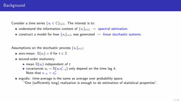
Consider a time series {xt ∈ C}t∈Z. The interest is to:
understand the information content of {xt}t∈Z spectral estimation.
construct a model for how {xt}t∈Z was generated linear stochastic systems.
Assumptions on the stochastic process {xt}t∈Z:
zero-mean: E(xt) = 0 for t ∈ Zsecond-order stationery:
mean E(xt) independent of tcovariances ck = E(xtx
∗t−k) only depend on the time lag k.
Note that c−k = c∗k .
ergodic: time-average is the same as average over probability space.“One (sufficiently long) realization is enough to do estimation of statistical properties”.
4 / 29
Background
Consider a time series {xt ∈ C}t∈Z. The interest is to:
understand the information content of {xt}t∈Z spectral estimation.
construct a model for how {xt}t∈Z was generated linear stochastic systems.
Assumptions on the stochastic process {xt}t∈Z:
zero-mean: E(xt) = 0 for t ∈ Zsecond-order stationery:
mean E(xt) independent of tcovariances ck = E(xtx
∗t−k) only depend on the time lag k.
Note that c−k = c∗k .
ergodic: time-average is the same as average over probability space.“One (sufficiently long) realization is enough to do estimation of statistical properties”.
4 / 29

BackgroundSpectral Estimation
The power spectrum of a stochastic process is the energy distribution across frequencies of the process.
⇒
! !"# $ $"# % %"# &$!
!'
$!!#
$!!(
$!!&
$!!%
$!!$
For our process {xt}t∈Z it is defined as the positive function Φ(e iθ) on (−π, π] ∼ T,
ck :=1
2π
∫Te ikθΦ(e iθ)dθ, k ∈ Z ⇐⇒ Φ(e iθ) ∼
∞∑k=−∞
cke−ikθ
i.e., with the covariances as Fourier coefficients [1].
Estimation Methods:
Periodogram
Burg’s method/maximum entropy
Sparse methods
Applications:
Radar/Sonar
Speech analysis
Communications
[1] P. Stoica, and R.L. Moses. Spectral analysis of signals. Prentice Hall, 2005. 5 / 29

BackgroundLinear stochastic systems
Want a model for how {xt} is generated. One of the simplest, a linear dynamical system.
Linear system W (z)ut xt
{ut} is a Gaussian white noise process
Gaussian: ut is Gaussian for all t.White: flat power spectrum Φu(e iθ) ≡ 1.
W (z) is an autoregressive-moving-average (ARMA) filter
xt +n∑
k=1
ak xt−k =m∑
k=0
bk ut−k ⇔ W (z) =∑k∈Z
wkz−k =
∑mk=0 bk z
−k∑nk=0 ak z
−k=
b(z)
a(z)
We want to identify W (z) from the data {xt}.
6 / 29

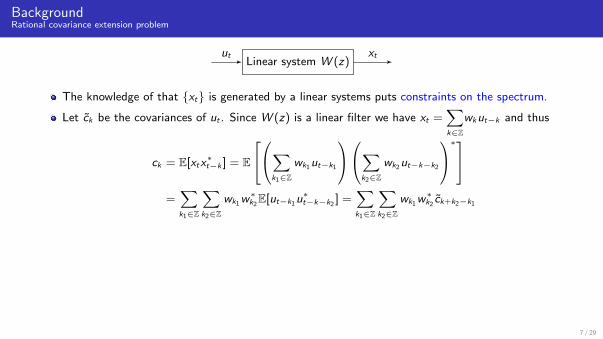
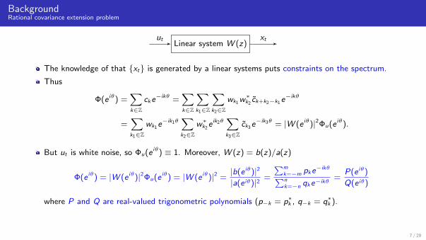
BackgroundRational covariance extension problem
Linear system W (z)ut xt
The knowledge of that {xt} is generated by a linear systems puts constraints on the spectrum.
7 / 29
BackgroundRational covariance extension problem
Linear system W (z)ut xt
The knowledge of that {xt} is generated by a linear systems puts constraints on the spectrum.
Let ck be the covariances of ut . Since W (z) is a linear filter we have xt =∑k∈Z
wkut−k and thus
ck = E[xtx∗t−k ] = E
∑k1∈Z
wk1ut−k1
∑k2∈Z
wk2ut−k−k2
∗=∑k1∈Z
∑k2∈Z
wk1w∗k2E[ut−k1u
∗t−k−k2
] =∑k1∈Z
∑k2∈Z
wk1w∗k2ck+k2−k1
7 / 29

BackgroundRational covariance extension problem
Linear system W (z)ut xt
The knowledge of that {xt} is generated by a linear systems puts constraints on the spectrum.
Let ck be the covariances of ut . Since W (z) is a linear filter we have xt =∑k∈Z
wkut−k and thus
ck = E[xtx∗t−k ] = E
∑k1∈Z
wk1ut−k1
∑k2∈Z
wk2ut−k−k2
∗=∑k1∈Z
∑k2∈Z
wk1w∗k2E[ut−k1u
∗t−k−k2
] =∑k1∈Z
∑k2∈Z
wk1w∗k2ck+k2−k1
Thus
Φ(e iθ) =∑k∈Z
cke−ikθ =
∑k∈Z
∑k1∈Z
∑k2∈Z
wk1w∗k2ck+k2−k1e
−ikθ
=∑k1∈Z
wk1e−ik1θ
∑k2∈Z
w∗k2e ik2θ
∑k3∈Z
ck3e−ik3θ = |W (e iθ)|2Φu(e iθ).
7 / 29

BackgroundRational covariance extension problem
Linear system W (z)ut xt
The knowledge of that {xt} is generated by a linear systems puts constraints on the spectrum.
Thus
Φ(e iθ) =∑k∈Z
cke−ikθ =
∑k∈Z
∑k1∈Z
∑k2∈Z
wk1w∗k2ck+k2−k1e
−ikθ
=∑k1∈Z
wk1e−ik1θ
∑k2∈Z
w∗k2e ik2θ
∑k3∈Z
ck3e−ik3θ = |W (e iθ)|2Φu(e iθ).
7 / 29
BackgroundRational covariance extension problem
Linear system W (z)ut xt
The knowledge of that {xt} is generated by a linear systems puts constraints on the spectrum.
Thus
Φ(e iθ) =∑k∈Z
cke−ikθ =
∑k∈Z
∑k1∈Z
∑k2∈Z
wk1w∗k2ck+k2−k1e
−ikθ
=∑k1∈Z
wk1e−ik1θ
∑k2∈Z
w∗k2e ik2θ
∑k3∈Z
ck3e−ik3θ = |W (e iθ)|2Φu(e iθ).
But ut is white noise, so Φu(e iθ) ≡ 1. Moreover, W (z) = b(z)/a(z)
Φ(e iθ) = |W (e iθ)|2Φu(e iθ) = |W (e iθ)|2 =|b(e iθ)|2
|a(e iθ)|2 =
∑mk=−m pke
−ikθ∑nk=−n qke
−ikθ=
P(e iθ)
Q(e iθ)
where P and Q are real-valued trigonometric polynomials (p−k = p∗k , q−k = q∗k ).
7 / 29

BackgroundRational covariance extension problem
Linear system W (z)ut xt
Summarizing, this gives us the following problem posed by Kalman [1]:
Problem formulation – Rational covariance extension problem
Given a sequence of covariances c = {ck}nk=−n find a positive function Φ(e iθ) so thatck =
1
2π
∫Te ikθΦ(e iθ)dθ, k = −n, . . . , 0, 1, . . . , n
Φ(e iθ) =P(e iθ)
Q(e iθ), P and Q ∈ P1
+.
Notation for nonnegative trigonometric polynomials:
P1+ = {p := {pk}nk=−n ∈ C2n+1 | p−k = p∗k , P(e iθ) :=
n∑k=−n
pke−ikθ, P(e iθ) ≥ 0 for all θ ∈ T}
[1] R.E. Kalman. Realization of covariance sequences. In the Proceedings of the Toeplitz Memorial Conference, 1981.
7 / 29

BackgroundRational covariance extension - spectral factorization and positive real functions
Key property in the identification: spectral factorization
P(e iθ)
Q(e iθ)
Spectral factorization→=←
Trivial
|b(e iθ)|2
|a(e iθ)|2
Intermission - Connection to analytic interpolation: equivalently characterized as finding a functionf (z) that is positive real and of specified degree, i.e.,
analytic in DC , i.e., f (z) =∞∑k=0
fkz−k for |z | > 1,
f (z) + f ∗(1/z∗) > 0 on T (f (z) + f ∗(1/z∗) = Φ(z) on T) ,
f (z) takes the form
f (z) =b(z)
a(z),
for a, b monic and of degree n and m, with roots inside the unit disc (Schur polynomials),
fulfilling f0 = 12c0 and fk = ck for k = 1, . . . , n. This gives interpolation conditions in infinity.
8 / 29

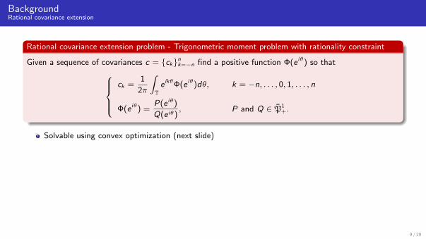
BackgroundRational covariance extension
Rational covariance extension problem - Trigonometric moment problem with rationality constraint
Given a sequence of covariances c = {ck}nk=−n find a positive function Φ(e iθ) so thatck =
1
2π
∫Te ikθΦ(e iθ)dθ, k = −n, . . . , 0, 1, . . . , n
Φ(e iθ) =P(e iθ)
Q(e iθ), P and Q ∈ P1
+.
Solvable using convex optimization (next slide)
Solution exists if and only if
T (c) =
c0 c−1 . . . c−n
c1 c0 . . . c−n+1
.... . .
...cn cn−1 . . . c0
� 0.
9 / 29

BackgroundRational covariance extension
Theorem ([1])
The rational covariance extension problem has a solution if only if T (c) � 0. For such c and anyP ∈ P1
+, there is a unique Q such that Φ = P/Q is a solution to the rational covariance extensionproblem.
Moreover, Φ = P/Q is the optimal solution to the convex problem
(P) minΦ≥0
∫TP log
P
Φ
dθ
2π
subject to ck =
∫Te ikθΦ(e iθ)
dθ
2πk = −n, . . . , 0, 1, . . . , n.
Finally, this Q is the unique solution to the dual problem
(D) minq∈P+
〈c, q〉 −∫TP log(Q)
dθ
2π.
[1] C.I. Byrnes, S.V. Gusev, and A. Lindquist. A convex optimization approach to the rational covariance extension problem. SIAM Journal on Control and Optimization 37(1),211-229, 1998.
10 / 29

BackgroundRational covariance extension
Theorem ([1])
The rational covariance extension problem has a solution if only if T (c) � 0. For such c and anyP ∈ P1
+, there is a unique Q such that Φ = P/Q is a solution to the rational covariance extensionproblem. Moreover, Φ = P/Q is the optimal solution to the convex problem
(P) minΦ≥0
∫TP log
P
Φ
dθ
2π
subject to ck =
∫Te ikθΦ(e iθ)
dθ
2πk = −n, . . . , 0, 1, . . . , n.
Finally, this Q is the unique solution to the dual problem
(D) minq∈P+
〈c, q〉 −∫TP log(Q)
dθ
2π.
[1] C.I. Byrnes, S.V. Gusev, and A. Lindquist. A convex optimization approach to the rational covariance extension problem. SIAM Journal on Control and Optimization 37(1),211-229, 1998.
10 / 29
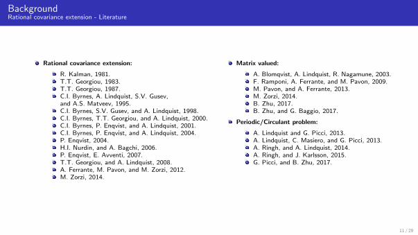
BackgroundRational covariance extension - Literature
Rational covariance extension:
R. Kalman, 1981.T.T. Georgiou, 1983.T.T. Georgiou, 1987.C.I. Byrnes, A. Lindquist, S.V. Gusev,and A.S. Matveev, 1995.C.I. Byrnes, S.V. Gusev, and A. Lindquist, 1998.C.I. Byrnes, T.T. Georgiou, and A. Lindquist, 2000.C.I. Byrnes, P. Enqvist, and A. Lindquist, 2001.C.I. Byrnes, P. Enqvist, and A. Lindquist, 2004.P. Enqvist, 2004.H.I. Nurdin, and A. Bagchi, 2006.P. Enqvist, E. Avventi, 2007.T.T. Georgiou, and A. Lindquist, 2008.A. Ferrante, M. Pavon, and M. Zorzi, 2012.M. Zorzi, 2014.
Matrix valued:
A. Blomqvist, A. Lindquist, R. Nagamune, 2003.F. Ramponi, A. Ferrante, and M. Pavon, 2009.M. Pavon, and A. Ferrante, 2013.M. Zorzi, 2014.B. Zhu, 2017.B. Zhu, and G. Baggio, 2017.
Periodic/Circulant problem:
A. Lindquist and G. Picci, 2013.A. Lindquist, C. Masiero, and G. Picci, 2013.A. Ringh, and A. Lindquist, 2014.A. Ringh, and J. Karlsson, 2015.G. Picci, and B. Zhu, 2017.
11 / 29

Multidimensional rational covariance extensionA multidimensional trigonometric moment problem
Trigonometric moment problem with rationality constraint
Given a sequence of covariances c = {ck}nk=−n find a positive function Φ(e iθ) so thatck =
1
2π
∫Te ikθΦ(e iθ)dθ, k = −n, . . . , 0, 1, . . . , n
Φ(e iθ) =P(e iθ)
Q(e iθ), P and Q ∈ P1
+.
12 / 29
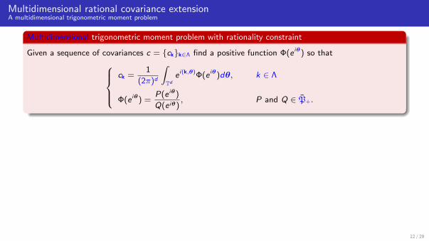
Multidimensional rational covariance extensionA multidimensional trigonometric moment problem
Multidimensional trigonometric moment problem with rationality constraint
Given a sequence of covariances c = {ck}k∈Λ find a positive function Φ(e iθ) so thatck =
1
(2π)d
∫Td
e i(k,θ)Φ(e iθ)dθ, k ∈ Λ
Φ(e iθ) =P(e iθ)
Q(e iθ), P and Q ∈ P+.
12 / 29

Multidimensional rational covariance extensionA multidimensional trigonometric moment problem
Multidimensional trigonometric moment problem with rationality constraint
Given a sequence of covariances c = {ck}k∈Λ find a positive function Φ(e iθ) so thatck =
∫Td
e i(k,θ)Φ(e iθ)dm, k ∈ Λ
Φ(e iθ) =P(e iθ)
Q(e iθ), P and Q ∈ P+.
dm = dθ/(2π)d
Λ ⊂ Zd is a index set with
0 ∈ Λ−Λ = Λ
E.g., the rectangular set Λ = {(k1, . . . , kd) ∈ Zd : |kj | ≤ nj , j = 1, . . . , d}
12 / 29

Multidimensional rational covariance extensionA multidimensional trigonometric moment problem
Multidimensional trigonometric moment problem with rationality constraint
Given a sequence of covariances c = {ck}k∈Λ find a positive function Φ(e iθ) so thatck =
∫Td
e i(k,θ)Φ(e iθ)dm, k ∈ Λ
Φ(e iθ) =P(e iθ)
Q(e iθ), P and Q ∈ P+.
dm = dθ/(2π)d
Λ ⊂ Zd is a index set with
0 ∈ Λ−Λ = Λ
E.g., the rectangular set Λ = {(k1, . . . , kd) ∈ Zd : |kj | ≤ nj , j = 1, . . . , d}Trigonometric polynomials P+:
P+ = {p := {pk}k∈Λ ∈ C|Λ| | p−k = p∗k , P(e iθ) :=∑k∈Λ
pke−i(k,θ), P(e iθ) ≥ 0 for all θ ∈ Td}
Compare to
P1+ = {p := {pk}nk=−n ∈ C2n+1 | p−k = p∗k , P(e iθ) :=
n∑k=−n
pke−ikθ, P(e iθ) ≥ 0 for all θ ∈ T}
12 / 29

Multidimensional rational covariance extensionA multidimensional trigonometric moment problem
Important notions for later:
∂P+ denotes the boundary of the set of nonnegative trigonometric polynomials, i.e., p ∈ P+ suchthat P(e iθ) = 0 in at least one point θ ∈ Td .
P+ is a cone: for all p1, p2 ∈ P+ we have that αp1 + βp2 ∈ P+ for any α, β ≥ 0. To see this
αp1 + βp2 ∑k∈Λ
(αp1k + βp2
k)e−i(k,θ) = αP1(e iθ) + βP2(e iθ) ≥ 0 ∀θ ∈ Td .
13 / 29

Multidimensional rational covariance extensionA multidimensional trigonometric moment problem
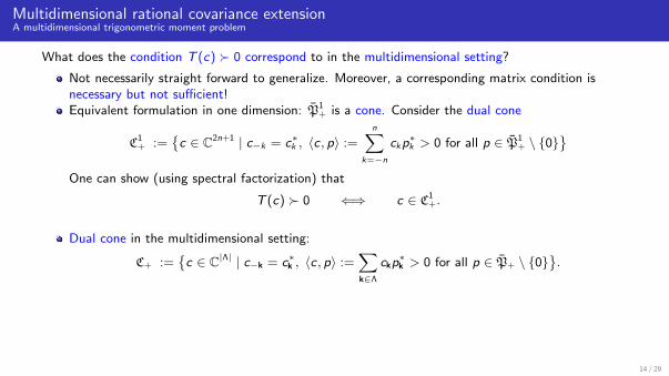
What does the condition T (c) � 0 correspond to in the multidimensional setting?
Not necessarily straight forward to generalize. Moreover, a corresponding matrix condition isnecessary but not sufficient!Equivalent formulation in one dimension: P1
+ is a cone. Consider the dual cone
C1+ :=
{c ∈ C2n+1 | c−k = c∗k , 〈c, p〉 :=
n∑k=−n
ckp∗k > 0 for all p ∈ P1
+ \ {0}}
One can show (using spectral factorization) that
T (c) � 0 ⇐⇒ c ∈ C1+.
Dual cone in the multidimensional setting:
C+ :={c ∈ C|Λ| | c−k = c∗k , 〈c, p〉 :=
∑k∈Λ
ckp∗k > 0 for all p ∈ P+ \ {0}
}.
Finally, the theory turns out to not be directly generalizable. Need to allow for solutions that aremeasures of bounded variation of the form
dµ(θ) = Φ(e iθ)dm + dν(θ),
where Φ = P/Q and dν is singular with respect to dm (Lebesgue decomposition).
14 / 29

Multidimensional rational covariance extensionA multidimensional trigonometric moment problem
What does the condition T (c) � 0 correspond to in the multidimensional setting?
Not necessarily straight forward to generalize. Moreover, a corresponding matrix condition isnecessary but not sufficient!
Equivalent formulation in one dimension: P1+ is a cone. Consider the dual cone
C1+ :=
{c ∈ C2n+1 | c−k = c∗k , 〈c, p〉 :=
n∑k=−n
ckp∗k > 0 for all p ∈ P1
+ \ {0}}
One can show (using spectral factorization) that
T (c) � 0 ⇐⇒ c ∈ C1+.
Dual cone in the multidimensional setting:
C+ :={c ∈ C|Λ| | c−k = c∗k , 〈c, p〉 :=
∑k∈Λ
ckp∗k > 0 for all p ∈ P+ \ {0}
}.
Finally, the theory turns out to not be directly generalizable. Need to allow for solutions that aremeasures of bounded variation of the form
dµ(θ) = Φ(e iθ)dm + dν(θ),
where Φ = P/Q and dν is singular with respect to dm (Lebesgue decomposition).
14 / 29

Multidimensional rational covariance extensionA multidimensional trigonometric moment problem
What does the condition T (c) � 0 correspond to in the multidimensional setting?
Not necessarily straight forward to generalize. Moreover, a corresponding matrix condition isnecessary but not sufficient!Equivalent formulation in one dimension: P1
+ is a cone. Consider the dual cone
C1+ :=
{c ∈ C2n+1 | c−k = c∗k , 〈c, p〉 :=
n∑k=−n
ckp∗k > 0 for all p ∈ P1
+ \ {0}}
One can show (using spectral factorization) that
T (c) � 0 ⇐⇒ c ∈ C1+.
Dual cone in the multidimensional setting:
C+ :={c ∈ C|Λ| | c−k = c∗k , 〈c, p〉 :=
∑k∈Λ
ckp∗k > 0 for all p ∈ P+ \ {0}
}.
Finally, the theory turns out to not be directly generalizable. Need to allow for solutions that aremeasures of bounded variation of the form
dµ(θ) = Φ(e iθ)dm + dν(θ),
where Φ = P/Q and dν is singular with respect to dm (Lebesgue decomposition).
14 / 29

Multidimensional rational covariance extensionA multidimensional trigonometric moment problem
What does the condition T (c) � 0 correspond to in the multidimensional setting?
Not necessarily straight forward to generalize. Moreover, a corresponding matrix condition isnecessary but not sufficient!Equivalent formulation in one dimension: P1
+ is a cone. Consider the dual cone
C1+ :=
{c ∈ C2n+1 | c−k = c∗k , 〈c, p〉 :=
n∑k=−n
ckp∗k > 0 for all p ∈ P1
+ \ {0}}
One can show (using spectral factorization) that
T (c) � 0 ⇐⇒ c ∈ C1+.
Dual cone in the multidimensional setting:
C+ :={c ∈ C|Λ| | c−k = c∗k , 〈c, p〉 :=
∑k∈Λ
ckp∗k > 0 for all p ∈ P+ \ {0}
}.
Finally, the theory turns out to not be directly generalizable. Need to allow for solutions that aremeasures of bounded variation of the form
dµ(θ) = Φ(e iθ)dm + dν(θ),
where Φ = P/Q and dν is singular with respect to dm (Lebesgue decomposition). 14 / 29

Multidimensional rational covariance extensionResults for exact covariance matching
Theorem
The multidimensional rational covariance extension problem has a solution only if c ∈ C+.
Moreover,for any c ∈ C+ and any P ∈ P+, any rational solution Φ = P/Q can be obtained by solving the convexprimal problem
(P) mindµ≥0
∫Td
(P log
P
Φdm + dµ− Pdm
)subject to ck =
∫Td
e i(k,θ)(
Φ(e iθ)dm + dν), k ∈ Λ.
Finally, for any c ∈ C+ problem (P) has a solution and it is given by
d µ =P(e iθ)
Q(e iθ)dm + d ν
where Q is the unique solution to the dual problem
(D) minq∈P+
〈c, q〉 −∫Td
P log(Q)dm.
and d ν is such that supp(d ν) ⊂ {θ ∈ Td | Q(e iθ) = 0}.
15 / 29

Multidimensional rational covariance extensionResults for exact covariance matching
Theorem
The multidimensional rational covariance extension problem has a solution only if c ∈ C+. Moreover,for any c ∈ C+ and any P ∈ P+, any rational solution Φ = P/Q can be obtained by solving the convexprimal problem
(P) mindµ≥0
∫Td
(P log
P
Φdm + dµ− Pdm
)subject to ck =
∫Td
e i(k,θ)(
Φ(e iθ)dm + dν), k ∈ Λ.
Finally, for any c ∈ C+ problem (P) has a solution and it is given by
d µ =P(e iθ)
Q(e iθ)dm + d ν
where Q is the unique solution to the dual problem
(D) minq∈P+
〈c, q〉 −∫Td
P log(Q)dm.
and d ν is such that supp(d ν) ⊂ {θ ∈ Td | Q(e iθ) = 0}.15 / 29

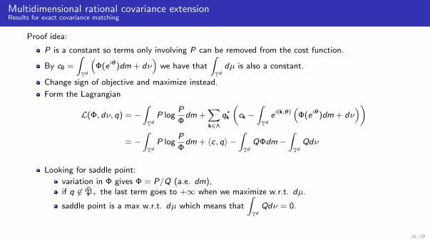
Multidimensional rational covariance extensionResults for exact covariance matching
Proof idea:
P is a constant so terms only involving P can be removed from the cost function.
By c0 =
∫Td
(Φ(e iθ)dm + dν
)we have that
∫Td
dµ is also a constant.
Change sign of objective and maximize instead.
Form the Lagrangian
L(Φ, dν, q) = −∫Td
P logP
Φdm +
∑k∈Λ
q∗k
(ck −
∫Td
e i(k,θ)(
Φ(e iθ)dm + dν))
= −∫Td
P logP
Φdm + 〈c, q〉 −
∫Td
QΦdm −∫Td
Qdν
Looking for saddle point:
variation in Φ gives Φ = P/Q (a.e. dm),if q 6∈ P+ the last term goes to +∞ when we maximize w.r.t. dµ.
saddle point is a max w.r.t. dµ which means that
∫Td
Qdν = 0.
Plugging this into the Lagrangian gives the dual problem (D).
16 / 29

Multidimensional rational covariance extensionResults for exact covariance matching
Proof idea (cont.):
Show existence and uniqueness of solution to (D):lower semi-continuity of the dual objective,compact sublevel sets,positive definite second variation.
Existence of a singular measure with supp(d ν) ⊂ {θ ∈ Td | Q(e iθ) = 0} so that
ck =
∫Td
e i(k,θ) P
Qdm + d ν.
Finally: sufficiency of the saddle point property for strong duality gives the result.
Why did we need the extension to dµ = Φdm + dν?
Derivative of the dual objective function J(q) = 〈c, q〉 −∫Td
P log(Q)dm:
∂J∂qk
= ck −∫Td
e i(k,θ) P
Qdm.
For d = 1, and also d = 2, this is infinite for Q ∈ ∂P+. So the solution is strictly in the interior, i.e.,Q(e iθ) > 0 for all θ ∈ Td
17 / 29

Multidimensional rational covariance extensionResults for approximate covariance matching
If c 6∈ C+, what can we do?
Inverse problems view: the primal problem
(P) mindµ≥0
∫Td
(P log
P
Φdm + dµ− Pdm
)subject to ck =
∫Td
e i(k,θ)(
Φ(e iθ)dm + dν), k ∈ Λ.
is on the form
mindµ≥0
I(dµ)
subject to dµ matches c exactly,
where the regularizer I promotes rational solutions. Change data-matching term.
18 / 29

Multidimensional rational covariance extensionResults for approximate covariance matching
Theorem
Given a sequence c = {ck}k∈Λ, for ε large enough the primal problem
(P ′) minΦ>0, r
∫Td
(P log
P
Φdm + dµ− Pdm
)subject to rk =
∫Td
e i(k,θ)(
Φ(e iθ)dm + dν), k ∈ Λ,
‖r − c‖2 ≤ ε2,
has an optimal solution given by
d µ =P(e iθ)
Q(e iθ)dm + d ν
where Q is the unique solution to the dual problem
(D ′) minq∈P+
〈c, q〉 −∫Td
P log(Q)dm + ε‖q − e‖,
and d ν is such that supp(d ν) ⊂ {θ ∈ Td | Q(e iθ) = 0}. Here, e ∈ C|Λ|, e0 = 1 and ek = 0 fork ∈ Λ \ {0}.
19 / 29

Outline
Background
Spectral estimationIdentification of stochastic linear systemsRational covariance extension
Multidimensional rational covariance extension
A multidimensional trigonometric moment problemResults for exact covariance matchingResults for approximate covariance matching
Example
Texture generation by Wiener system identification
20 / 29

ExampleTexture generation by Wiener system identification
Motivated by the use of thresholded Gaussian random fields to model porous materials [1], we areinterested in generating binary textures.
We want to estimate a system that can generate similar textures multidimensional Wiener systems identification.
Figure: Example of a texture
[1] S. Eriksson Barman. Gaussian random field based models for the porous structure of pharmaceutical film coatings. In Acta Stereologica [En ligne], Proceedings ICSIA, 14thICSIA abstracts, 2015. 21 / 29

ExampleTexture generation by Wiener system identification
Motivated by the use of thresholded Gaussian random fields to model porous materials [1], we areinterested in generating binary textures.We want to estimate a system that can generate similar textures multidimensional Wiener systems identification.
Figure: Example of a texture
[1] S. Eriksson Barman. Gaussian random field based models for the porous structure of pharmaceutical film coatings. In Acta Stereologica [En ligne], Proceedings ICSIA, 14thICSIA abstracts, 2015. 21 / 29

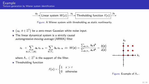
ExampleTexture generation by Wiener system identification
Linear system W (z) Threholding function f (x)ut xt yt
Figure: A Wiener system with thresholding as static nonlinearity.
{ut ; t ∈ Z2} be a zero-mean Gaussian white noise input.
The linear dynamical system is a strictly causalautoregressive-moving-average (ARMA) filter
xt +∑
k∈Λ+\{0}
ak xt−k =∑k∈Λ+
bk ut−k ⇔ W (z) =
∑k∈Λ+
bk zk∑
k∈Λ+ak zk
=b(z)
a(z)
where Λ+ ⊂ Z2 is the support of the filter.
Thresholding function
f (x) =
{1 x > τ
0 otherwise
k1
k2
Figure: Example of Λ+.
Goal: From samples (yt) we want to identify τ and W .
22 / 29

ExampleTexture generation by Wiener system identification
Linear system W (z) Threholding function f (x)ut xt yt
Figure: A Wiener system with thresholding as static nonlinearity.
{ut ; t ∈ Z2} be a zero-mean Gaussian white noise input.
The linear dynamical system is a strictly causalautoregressive-moving-average (ARMA) filter
xt +∑
k∈Λ+\{0}
ak xt−k =∑k∈Λ+
bk ut−k ⇔ W (z) =
∑k∈Λ+
bk zk∑
k∈Λ+ak zk
=b(z)
a(z)
where Λ+ ⊂ Z2 is the support of the filter.
Thresholding function
f (x) =
{1 x > τ
0 otherwise
k1
k2
Figure: Example of Λ+.
Goal: From samples (yt) we want to identify τ and W .22 / 29

ExampleTexture generation by Wiener system identification
Linear system W (z) Threholding function f (x)ut xt yt
Figure: A Wiener system with thresholding as static nonlinearity.
Identifying the threshold parameter:Since ut is zero-mean and Gaussian and W (z) is linear, xt is zero-mean and Gaussian.In steady-state xt is second order stationary process, i.e., the covariances are independent ofthe absolute time t: ck := E[xtxt−k]. Assume that E[xtxt ] = c0 = 1 (normalization).E[yt ] = P(yt = 1) = P(xt > τ) = 1− P(xt ≤ τ) = 1− φ(τ), where φ is the Gaussian CDF we can estimate τ as τest = φ−1(1− E[yt ]).
Estimate covariances ck:Let rk := E[yt−kyt ]− E[yt−k]E[yt ] be the covariances of the process yt .Since xt is Gaussian a theorem by Price [1] gives the following relationship between thecovariances
rk =
∫ ck
0
1
2π√
1− s2exp
(− τ 2
1 + s
)ds.
Since the integrand is positive, the mapping can be inverted (numerically).From the covariances ck, estimate the linear system W (z).
[1] R. Price. A useful theorem for nonlinear devices having Gaussian inputs. IRE Transactions on Information Theory, 4(2), 69-72, 1958.
23 / 29

ExampleTexture generation by Wiener system identification
Linear system W (z) Threholding function f (x)ut xt yt
Figure: A Wiener system with thresholding as static nonlinearity.
Identifying the threshold parameter:Since ut is zero-mean and Gaussian and W (z) is linear, xt is zero-mean and Gaussian.
In steady-state xt is second order stationary process, i.e., the covariances are independent ofthe absolute time t: ck := E[xtxt−k]. Assume that E[xtxt ] = c0 = 1 (normalization).E[yt ] = P(yt = 1) = P(xt > τ) = 1− P(xt ≤ τ) = 1− φ(τ), where φ is the Gaussian CDF we can estimate τ as τest = φ−1(1− E[yt ]).
Estimate covariances ck:Let rk := E[yt−kyt ]− E[yt−k]E[yt ] be the covariances of the process yt .Since xt is Gaussian a theorem by Price [1] gives the following relationship between thecovariances
rk =
∫ ck
0
1
2π√
1− s2exp
(− τ 2
1 + s
)ds.
Since the integrand is positive, the mapping can be inverted (numerically).From the covariances ck, estimate the linear system W (z).
[1] R. Price. A useful theorem for nonlinear devices having Gaussian inputs. IRE Transactions on Information Theory, 4(2), 69-72, 1958.
23 / 29
ExampleTexture generation by Wiener system identification
Linear system W (z) Threholding function f (x)ut xt yt
Figure: A Wiener system with thresholding as static nonlinearity.
Identifying the threshold parameter:Since ut is zero-mean and Gaussian and W (z) is linear, xt is zero-mean and Gaussian.In steady-state xt is second order stationary process, i.e., the covariances are independent ofthe absolute time t: ck := E[xtxt−k]. Assume that E[xtxt ] = c0 = 1 (normalization).
E[yt ] = P(yt = 1) = P(xt > τ) = 1− P(xt ≤ τ) = 1− φ(τ), where φ is the Gaussian CDF we can estimate τ as τest = φ−1(1− E[yt ]).
Estimate covariances ck:Let rk := E[yt−kyt ]− E[yt−k]E[yt ] be the covariances of the process yt .Since xt is Gaussian a theorem by Price [1] gives the following relationship between thecovariances
rk =
∫ ck
0
1
2π√
1− s2exp
(− τ 2
1 + s
)ds.
Since the integrand is positive, the mapping can be inverted (numerically).From the covariances ck, estimate the linear system W (z).
[1] R. Price. A useful theorem for nonlinear devices having Gaussian inputs. IRE Transactions on Information Theory, 4(2), 69-72, 1958.
23 / 29

ExampleTexture generation by Wiener system identification
Linear system W (z) Threholding function f (x)ut xt yt
Figure: A Wiener system with thresholding as static nonlinearity.
Identifying the threshold parameter:Since ut is zero-mean and Gaussian and W (z) is linear, xt is zero-mean and Gaussian.In steady-state xt is second order stationary process, i.e., the covariances are independent ofthe absolute time t: ck := E[xtxt−k]. Assume that E[xtxt ] = c0 = 1 (normalization).E[yt ] = P(yt = 1) = P(xt > τ) = 1− P(xt ≤ τ) = 1− φ(τ), where φ is the Gaussian CDF we can estimate τ as τest = φ−1(1− E[yt ]).
Estimate covariances ck:Let rk := E[yt−kyt ]− E[yt−k]E[yt ] be the covariances of the process yt .Since xt is Gaussian a theorem by Price [1] gives the following relationship between thecovariances
rk =
∫ ck
0
1
2π√
1− s2exp
(− τ 2
1 + s
)ds.
Since the integrand is positive, the mapping can be inverted (numerically).From the covariances ck, estimate the linear system W (z).
[1] R. Price. A useful theorem for nonlinear devices having Gaussian inputs. IRE Transactions on Information Theory, 4(2), 69-72, 1958.
23 / 29

ExampleTexture generation by Wiener system identification
Linear system W (z) Threholding function f (x)ut xt yt
Figure: A Wiener system with thresholding as static nonlinearity.
Identifying the threshold parameter:Since ut is zero-mean and Gaussian and W (z) is linear, xt is zero-mean and Gaussian.In steady-state xt is second order stationary process, i.e., the covariances are independent ofthe absolute time t: ck := E[xtxt−k]. Assume that E[xtxt ] = c0 = 1 (normalization).E[yt ] = P(yt = 1) = P(xt > τ) = 1− P(xt ≤ τ) = 1− φ(τ), where φ is the Gaussian CDF we can estimate τ as τest = φ−1(1− E[yt ]).
Estimate covariances ck:Let rk := E[yt−kyt ]− E[yt−k]E[yt ] be the covariances of the process yt .Since xt is Gaussian a theorem by Price [1] gives the following relationship between thecovariances
rk =
∫ ck
0
1
2π√
1− s2exp
(− τ 2
1 + s
)ds.
Since the integrand is positive, the mapping can be inverted (numerically).
From the covariances ck, estimate the linear system W (z).
[1] R. Price. A useful theorem for nonlinear devices having Gaussian inputs. IRE Transactions on Information Theory, 4(2), 69-72, 1958.23 / 29

ExampleTexture generation by Wiener system identification
Linear system W (z) Threholding function f (x)ut xt yt
Figure: A Wiener system with thresholding as static nonlinearity.
Identifying the threshold parameter:Since ut is zero-mean and Gaussian and W (z) is linear, xt is zero-mean and Gaussian.In steady-state xt is second order stationary process, i.e., the covariances are independent ofthe absolute time t: ck := E[xtxt−k]. Assume that E[xtxt ] = c0 = 1 (normalization).E[yt ] = P(yt = 1) = P(xt > τ) = 1− P(xt ≤ τ) = 1− φ(τ), where φ is the Gaussian CDF we can estimate τ as τest = φ−1(1− E[yt ]).
Estimate covariances ck:Let rk := E[yt−kyt ]− E[yt−k]E[yt ] be the covariances of the process yt .Since xt is Gaussian a theorem by Price [1] gives the following relationship between thecovariances
rk =
∫ ck
0
1
2π√
1− s2exp
(− τ 2
1 + s
)ds.
Since the integrand is positive, the mapping can be inverted (numerically).From the covariances ck, estimate the linear system W (z).
[1] R. Price. A useful theorem for nonlinear devices having Gaussian inputs. IRE Transactions on Information Theory, 4(2), 69-72, 1958.23 / 29

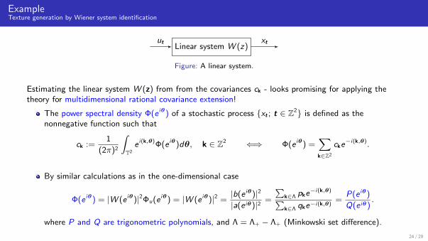
ExampleTexture generation by Wiener system identification
Linear system W (z)ut xt
Figure: A linear system.
Estimating the linear system W (z) from from the covariances ck - looks promising for applying thetheory for multidimensional rational covariance extension!
The power spectral density Φ(e iθ) of a stochastic process {xt ; t ∈ Z2} is defined as thenonnegative function such that
ck :=1
(2π)2
∫T2
e i(k,θ)Φ(e iθ)dθ, k ∈ Z2 ⇐⇒ Φ(e iθ) =∑k∈Z2
cke−i(k,θ).
By similar calculations as in the one-dimensional case
Φ(e iθ) = |W (e iθ)|2Φu(e iθ) = |W (e iθ)|2 =|b(e iθ)|2
|a(e iθ)|2 =
∑k∈Λ pke
−i(k,θ)∑k∈Λ qke
−i(k,θ)=
P(e iθ)
Q(e iθ).
where P and Q are trigonometric polynomials, and Λ = Λ+ − Λ+ (Minkowski set difference).
24 / 29

ExampleTexture generation by Wiener system identification
Pointed out earlier: in one dimension, spectral factorization as a sum-of-one-square:
P(e iθ)
Q(e iθ)
Spectral factorization→=←
Trivial
|b(e iθ)|2
|a(e iθ)|2
Not true in the higher dimensions - only factorization as sum-of-several-squares can be guaranteed[1, 2]:
P(e iθ)
Q(e iθ)=
∑`k=1 |bk(e iθ)|2∑mk=1 |ak(e iθ)|2 .
Open question: how to construct a realization from such a spectrum?
We resort to a heuristic, obtained by “abusing” results in [3].
[1] M.A. Dritschel. On factorization of trigonometric polynomials. Integral Equations and Operator Theory, 49(1), 11-42, 2004.
[2] J.S. Geronimo, and M.J. Lai. Factorization of multivariate positive Laurent polynomials. Journal of Approximation Theory, 139(1-2), 327-345, 2006.
[3] J.S. Geronimo, and H.J. Woerdeman. Positive extensions, Fejer-Riesz factorization and autoregressive filters in two variables. Annals of Mathematics, 839-906, 2004.
25 / 29

ExampleTexture generation by Wiener system identification
Linear system W (z) Threholding function f (x)ut xt yt
Figure: A Wiener system with thresholding as static nonlinearity.
Algorithm for Wiener system identification with thresholding
Input: (yt)1: Estimate threshold parameter: τest = φ−1(1− E [yt ]) from the data.2: Estimate covariances: rk := E [yt−kyt ]− E [yt−k]E [yt ] from the data.
3: Compute covariances ck := E [xt−kxt ] by using the relation rk =
∫ ck
0
1
2π√
1− s2exp
(− τ 2
1 + s
)ds
4: Estimate a rational spectrum using the theory developed here.5: Apply a heuristic, approximate factorization procedure.
Output: τest, coefficients for the linear dynamical system
26 / 29

ExampleTexture generation by Wiener system identification
(a) Texture. (b) Reconstruction.
(c) Close-up of the texture. (d) Close-up of the reconstruction. 27 / 29

ExampleTexture generation by Wiener system identification
(e) Texture. (f) Reconstruction.
(g) Close-up of the texture. (h) Close-up of the reconstruction. 27 / 29
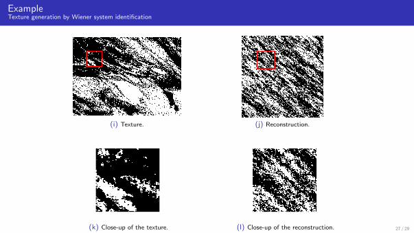
ExampleTexture generation by Wiener system identification
(i) Texture. (j) Reconstruction.
(k) Close-up of the texture. (l) Close-up of the reconstruction. 27 / 29
Conclusion and future work
Conclusions:
Rational covariance extension - motivated from identification of a linear stochastic system
Trigonometric moment problem view and convex optimization problem generalized tomultidimensional problems
We can do estimation of rational multidimensional spectra + impulses using convexoptimizationRelaxation of exact covariance matching criteria
Example in Wiener system identification for binary texture generation
Future work/open issues:
Why do we need a singular measure in dimensions d ≥ 3?
What does a spectrum
P(e iθ)
Q(e iθ)=
∑`k=1 |bk(e iθ)|2∑mk=1 |ak(e iθ)|2
represent in terms of dynamical systems in dimensions d ≥ 2?
Good method for approximation as a sum-of-one square?
28 / 29

Thank you for your attention!
Questions?
29 / 29