The Nonparametric Approach to Demand Analysis

Hal R. Varian

Econometrica, Vol. 50, No. 4. (Jul., 1982), pp. 945-973.

Stable URL:

http://links.jstor.org/sici?sici=0012-9682%28198207%2950%3A4%3C945%3ATNATDA%3E2.0.CO%3B2-O

Econometrica is currently published by The Econometric Society.

Your use of the JSTOR archive indicates your acceptance of JSTOR's Terms and Conditions of Use, available athttp://www.jstor.org/about/terms.html. JSTOR's Terms and Conditions of Use provides, in part, that unless you have obtainedprior permission, you may not download an entire issue of a journal or multiple copies of articles, and you may use content inthe JSTOR archive only for your personal, non-commercial use.

Please contact the publisher regarding any further use of this work. Publisher contact information may be obtained athttp://www.jstor.org/journals/econosoc.html.

Each copy of any part of a JSTOR transmission must contain the same copyright notice that appears on the screen or printedpage of such transmission.

The JSTOR Archive is a trusted digital repository providing for long-term preservation and access to leading academicjournals and scholarly literature from around the world. The Archive is supported by libraries, scholarly societies, publishers,and foundations. It is an initiative of JSTOR, a not-for-profit organization with a mission to help the scholarly community takeadvantage of advances in technology. For more information regarding JSTOR, please contact support@jstor.org.

http://www.jstor.orgWed Feb 27 17:24:30 2008

Econorneirica, Vol. 50, No. 4 (July. 1982)

THE NONPARAMETRIC APPROACH TO DEMAND ANALYSIS

This paper shows how to test data for consistency with utility maximization, recover the underlying preferences, and forecast demand behavior without making any assumptions concerning the parametric form of the underlying utility or demand functions.

THE ECONOMIC THEORY of consumer demand is extremely simple. The basic behavioral hypothesis is that the consumer chooses a bundle of goods that is preferred to all other bundles that he can afford. Applied demand analysis typically addresses three sorts of issues concerning this behavioral hypothesis.

(i) Consistency. When is observed behavior consistent with the preference maximization model?

(ii) Recoverability. How can we recover preferences given observations on consumer behavior?

(iii) Extrapolation. Given consumer behavior for some price configurations how can we forecast behavior for other price configurations?

The standard approach to these questions proceeds by postulating parametric forms for the demand functions and fitting them to observed data. The estimated demand functions can then be tested for consistency with the maximization hypothesis, used to make welfare judgements, or used to forecast demand for other price configurations. This procedure will be satisfactory only when the postulated parametric forms are good approximations to the "true" demand functions. Since this hypothesis is not directly testable, it must be taken on faith.

In this paper I describe an alternative approach to the above problems in consumer demand analysis. The proposed approach is nonparametric in that it requires no ad hoc specifications of functional forms for demand equations. Rather, the nonparametric approach deals with the raw demand data itself using techniques of finite mathematics. In particular I will show how one can directly and simply test a finite body of data for consistency with preference maximiza- tion, recover the underlying preferences in a variety of formats, and use them to extrapolate demand behavior to new price configurations. Thus each of the issues of concern to demand analysis mentioned above is amenable to the nonparamet- ric approach.2

1. TESTING FOR CONSISTENCY WITH THE MAXIMIZATION HYPOTHESIS

Letp ' = ( p ; , . . . ,pL) denote the ith observation of the prices of some k goods and let x ' = (x ; , . . . ,xk) be the associated quantities. Suppose that we have n

'This work was financed by grants from the National Science Foundation and the Guggenheim Memorial Foundation. I wish to thank Erwin Diewert, Avinash Dixit, Joseph Farrell, Angus Deaton, and Sydney Afriat for comments on an earlier draft.

2Another concern of applied demand analysis is the issue of testing for restrictions on the form of the utility function or budget constraint such as homotheticity, separability, etc. I address these questions in Varian [29, 301.

946 HAL R.VARIAN

observations on these prices and quantities, (pi ,xi) , i = 1, . . . ,n. How can we tell if these observations could have been generated by a neoclassical, utility maximizing consumer?

DEFINITION:A utility function u(x) rationalizes a set of observations (p ', x '), i = 1 , . . . , n , if u ( x i ) 2 u ( x ) f o r a l l x such t ha tp ix i2p ix .

At the most general level there is a very simple answer to the above question: any finite number of observations can be rationalized by the trivial constant utility function u(x) = 1 for all x. The real question is when can the observations be rationalized by a sufficiently well behaved nondegenerate utility function? The best results in this direction are due to Sydney Afriat [I,2,3,4,5].

AFRIAT'STHEOREM:The following conditions are equivalent: (1) There exists a nonsatiated utility function that rationalizes the data. (2) The data satisfies "cyclical consistency"; that is,

p rx r 2 p r x 3 , psxs 2pSx ' , . . . , p4x4 2 p 9 x r

implies

prxr =prxs, pSxS=psx', . . ) p9xq =pyxr.

(3) There exist numbers Ui, X i > 0, i = 1, . . . ,n, such that

U i S ~ J + X j p j ( x i - x i ) for i , j = l , . . . , n.

(4) There exists a nonsatiated, continuous, concave, monotonic utility function that rationalizes the data.

PROOF: See Appendix 1.

There are several remarkable features of Afriat's theorem. First, the equiva- lence of (1) and (4) shows that if some data can be rationalized by any nontrivial utility function at all it can in fact be rationalized by a very nice utility function. Or put another way, violations of continuity, concavity, or monotonicity cannot be detected with only a finite number of demand observations. Secondly, the numbers Ui and X i referred to in part (3) of Afriat's theorem can be used to actually construct a utility function that rationalizes the data. The numbers U' and X i can be interpreted as measures of the utility level and marginal utility of income at the observed demands. This is described in more detail in Appendix 1.

Thirdly, parts (2) and (3) of Afriat's theorem give directly testable conditions that the data must satisfy if it is to be consistent with the maximization model. Condition (3) for example simply asks whether there exists a nonnegative solution to a set of linear inequalities. The existence of such a solution can be checked by solving a linear program with 2n variables and n2 constraints. Diewert and Parkan [lo] describe some of their computational experience with this technique using actual demand data. Unfortunately the fact that the number

DEMAND ANALYSIS 947

of constraints rises as the square of the number of observations makes this condition difficult to verify in practice for computational reason^.^

Condition (2) seems rather more promising from the computational perspec- tive. As it turns out, there is an equivalent formulation of condition (2) which is quite easy to test. In addition this equivalent formulation is much more closely related to the traditional literature on the revealed preference approach to demand theory of Samuelson [24], Houthakker [12],Richter [21], and others. In order to describe this formulation we must first consider the following defini- tions:

DEFINITIONS:Given an observation x i and a bundle x : (1) x' is directly revealedpreferred to x , written x 'ROx,if pix' L p ' x . (2) x i is strictly directly revealed preferred to x , written x ' P O X , if pix ' > pix. (3) x i is revealed preferred to x , written x ' R x , if p ' x i L pix', pJx i

- . . . ,pn7x 2 pn'x for some sequence of observations ( x i , x J , . . . ,x " I ) .2 "' In this case we say that the relation R is the transitive closure of the relation RO.

(4) x' is strictly revealedpreferred to x , written x 'Px, if there exist observations x i and x i such that x iRxJ , xJpox l , X'RX.

Note that in the above definitions we do not require x ' , X I , x l , etc. to be distinct observations. We also adopt the convention that xRx for all bundles x .

DEFINITIONS:A set of data satisfies the: (1) Strong Axiom of Revealed Preference, version 1 (SARP 1) if X ' R X ~ and

xJRxl implies x' = x J ; (2) Strong Axiom of Revealed Preference, version 2 (SARP 2) if X'RXJand

x' # xJ implies not xJRx l ; (3) Strong Axiom of Revealed Preference, version 3 (SARP 3) if x lRxJ and

x ' # xJ implies not xjROx'; (4 ) Generalized Axiom of Revealed Preference (GARP) if x'RxJ implies not

XJPOX'.

The most common statement of the Strong Axiom is probably SARP 2.4 It is clear that SARP 1 is equivalent to SARP 2. It is not quite so clear that SARP 3 is equivalent to SARP 2, but nevertheless they are equivalent. One can easily show that SARP 1 , SARP 2, and SARP 3 imply GARP, but not vice versa. Basically SARP (in any of its formulations) requires single valued demand functions while GARP is compatible with multivalued dema.nd functions. For example, the data in Figure 1 violate SARP but are quite compatible with GARP.

'one can always use the duality theorem of linear programming to construct an equivalent problem with n2 variables and 2n constraints, but this problem may also be computationally difficult.

4 ~ e eRichter [22]for several variations on revealed preference axioms. Note that Richter considers a framework where the entire demand correspondence is given, rather than only a finite number of observations. This leads to a number of differences in the analysis.

HAL R.VARIAN

This is why we refer to GARP as the Generalized Axiom of Revealed Preference. It turns out to be a necessary and sufficient condition for data to be consistent with utility maximization, and is in fact equivalent to Afriat's cyclical consistency condition.

FACT 1 : A set of data satisfies cyclical consistency if and only if it satisfies GARP.

PROOF: Suppose that we have some data containing a violation of cyclical consistency so thatprxr 2 p r x " . . . ,pJxJ >pjx i , . . . ,pqxq 2pqxr . Then xiRxJ by going around the cycle, and xjpOxi directly. Hence we have a violation of GARP.

On the other hand, suppose we have some data that has a violation of GARP. Then writing out the violation in the above form shows we have a violation of cyclical consistency also.

The equivalency of GARP and cyclical consistency is trivial from the mathe- matical point of view, but is quite important from the computational point of view, since GARP is quite simple to check in practice, as we discuss below.

First, let us note that GARP can be restated as: if xiRxJ then pJxJ 5 pJxi for i, j = 1, . . . ,n. Hence verifying that some data satisfies GARP is trivial once we know the relation R-the transitive closure of the direct revealed preference relation R O.

It is clear that the computation of the transitive closure of a finite relation is a finite problem. The only issue is how one might compute it efficiently. This question has been addressed in the economics literature by Koo [14,15,16], Dobell [7], and Uebe [28],and in the computer science literature by Warshall [31] and Munroe [20], among others.

Most of the algorithms in the economics literature compute the transitive closure of a relation in time proportional to n4. The computer scientists, utilizing the law of comparative advantage, do a bit better. Warshall's algorithm computes the transitive closure in n3 steps, and Munroe describes a process that does it in time proportional to n2.74.Warshall's algorithm is especially easy to implement

949 DEMAND ANALYSIS

and quite ingenious. It seems fast enough for the problems encountered in economics, as well. We therefore describe Warshall's algorithm in Appendix 2.

At this point it might be worthwhile to be rather explicit about how one represents the relations R 0 and R in a form suitable for computation and how one actually verifies GARP in a systematic way.

Let us construct an n by n matrix M whose i - j entry is given by:

, , = 1 if p 'x ' 2 'xi, that is, x 'ROxJ;( 0 otherwise.

M is constructed directly from the data; it summarizes the relation RO.Warsh-all's algorithm, described in Appendix 2, operates on M to create a matrix MT where

,t, = 1 if X ' R X J ,40 otherwise.

MT can be used to check GARP in the following way.

ALGORITHM1: Checking data for consistency with GARP. Inputs: ( p i , x ' ) ,i = 1 , . . . , n, and the matrix MT representing the relation R. Outputs: whether the data satisfies GARP or not. 1. Is mtiJ= 1 and pJxJ>pJxi for some i and j? If so, we have a violation of

GARP.

Algorithm 1 is easily implemented on a computer. According to Afriat's theorem and Fact 1 we can use Algorithm 1 to simply and directly test a finite amount of data with the utility maximization model. If some data satisfies GARP then there is a nice utility function that will rationalize the observed behavior. If the data contains a violation of GARP then there does not exist a nonsatiated utility function that will rationalize the data. Hence we have a straightforward and efficient way to check a finite amount of data for consis- tency with the neoclassical model of consumer behavior.

2. RECOVERABILITY-ORDINAL COMPARISONS OF CONSUMPTION BUNDLES

Let us turn now to a somewhat different issue, namely the recoverability question described in the introduction. The revealed preference relation R which we discussed in the previous section summarizes all of the preference information contained in the demand observations. Any complete preference ordering that rationalizes the data must contain R, and every completion of R that rationalizes the data is a possible preference ordering that generated the data.

However, economists typically assume certain regularity conditions on the allowable preference orderings. For example we might restrict ourselves to preference orderings representable by utility functions that are nonsatiated,

950 HAL R. VARIAN

monotonic, and concave. Afriat's theorem implies that we can always impose such restrictions with no loss of generality; and conversely, that it is impossible to detect violations of these restrictions with a finite amount of demand data.

Suppose then that we are given two new consumption bundles x0 and x' that have not been previously observed. Suppose that every continuous, nonsatiated, concave, monotonic utility function u(x) that was consistent with (p l ,x l ) , i = 1, . . . , n, implied that u(xO) > u(x'). Then we might well be justified in concluding that x0 was in fact preferred to x'.

Alternatively we could adopt the following viewpoint. Suppose that every price vector po at which x0 could be demanded-and that was consistent with the data (pi,xi), i = 1, . . . , n-also implied that x0 was revealed preferred to x'. Then certainly we could conclude x0 would be preferred to x' by any consistent consumer. Let us consider this approach in a bit more detail.

First it is clear that if x0 has already been observed-so we know the price at which x0 is demanded-there is no problem in verifying whether X'RX'. Hence we concentrate on the case where x0 has not previously been observed. In this case we do not know what price to associate with x0 for purposes of the revealed preference comparison. However, we do know what the set of possible prices could be:

DEFINITION:Given any bundle x0 not previously observed we define the set of prices that support x0 by:

s (xO)= : (p l , x i ) , i = 0, . . . , n, satisfies GARP andp0x0 = 1 )

This is simply the set of prices at which x0 could be demanded and still be consistent with the previously observed behavior. (The requirement thatp0x0 = 1 is a convenient normalization.) We note that Afriat's theorem implies s(xO) is nonempty for all xO-just let p0 be the supporting price at x0 of any concave utility function that rationalizes the data.

We can use the definition of GARP to provide a convenient description of s(xO):

FACT 2: A price vector p0 is in s (xO) if and only if it satisfies the following system of linear inequalities:

pox05poxi for all x i such that x 'RX', (2)

pox0< pox ' for all x ' such that x 'pxO.

PROOF: Follows immediately from the definition of GARP.

DEMAND ANALYSIS 95 1

According to Fact 2, S(xO) is simply the solution set to a certain system of linear inequalities constructed from the data (pi,xi), i = 1, . . . , n, and the relations R and P.

We can use S(x) to describe the set of observations "revealed worse" than x0 and "revealed preferred" to x' in the following way.

R w(xO)= { x :for allp0 in ~ ( x ~ ) , p ~ x ~ 2 p 0 x i for

some xiPx or pox0 >poxi for some xiRx ),

RP(x') = { x :for allp in S(x) ,px 2 p x i for some

x'Px' orpx >?xi for some xiRx').

More succinctly, and with only a slight abuse of our earlier definitions, we might write:

RP(x') = { x : for allp in S(x), xPx')

These definitions formalize the idea described earlier: if x' is in R w(xO), then whatever the price at which x0 is demanded-as long as it is consistent with the previous data-that price will necessarily make x0 revealed preferred to x'. Thus every concave monotonic utility function that rationalizes the data must rank x0 ahead of x'. Of course RP(x') has a similar interpretation. In fact it is clear from the definitions that x0 is "revealed preferred" to x' if and only if x' is "revealed worse" than xO. We record this fact for future reference.

FACT3: x0 is in RP(x') i f and only i f x' is in Rw(xO).

Rp(xO) and R w(xO) are extremely important to the rest of our discussion so it is worthwhile presenting a few two-dimensional examples. The simplest case- with one data point-is presented in Figure 2. Let us verify that Figure 2 is correct.

First, we consider Rp(xO). In this simple case, Rp(xO) is simply the convex monotonic hull of all points revealed preferred to xO: namely x ' and x0 itself. To verify this, let x be any point in Rp(xO), and let p be any (nonnegative) price vector at which x could be demanded. It is geometrically clear that, whatever budget line is chosen, x will be revealed preferred to xO-either directly, or indirectly through the observation x'. (The reader might check his understanding of this point by indicating the region where x will be directly revealed preferred to x0 by all supporting prices, and the region where x will only be indirectly revealed preferred to x0 for some supporting prices.) So much for RP(x').

In order to verify the construction of Rw(xO), we have to consider all of the prices at which x0 could be demanded and still be consistent with the previous

HAL R. VARIAN

data point (p1,x') . In this case GARP imposes an important restriction on the budget line through x0 can be no steeper than the indicated angle 8. If it were steeper we would create a violation of GARP: we would have x'RxO, and xOPOX'. R w(xO) is the set of points that lie below all budget lines consistent with GARP -exactly as illustrated in Figure 2.

Figure 3 presents a more complex example. As before RP(xO) turns out to be the convex monotonic hull of all the points revealed preferred to xO. R w(xO) is a bit more interesting. For all budgets that support x0 and satisfy GARP, x0 is revealed preferred to x l , and a fortiori to all the points beneath xl 's budget set . . . including x2, x3 and so on.

Now Figure 3 presents us with quite a bit of information about the indiffer- ence curve passing through xO: it cannot intersect Rp(xO) or Rw(xo)-hence it must lie in between the two. Put another way, the set of bundles preferred to x0 (using the true utility function) must always contain RP(~') , and must be

953 DEMAND ANALYSIS

contained in the complement of R w ( x O ) .This last set, the complement of R w ( x O ) , will be useful later on; we will call it NR w ( x O )for "not revealed worse" than xO.

It is clear from Figure 3 that R p ( x O )and NRW(X') are not only "inner" and "outer" estimates of the set of bundles preferred to xO,they are also the tightest inner and outer estimates. If a point x' is not contained in either of these sets then there is a nice utility function that rationalizes the data for which u(xO) 2 u ( x l ) .. . and there is a nice utility function that rationalizes the data for which u ( x l )2 u(xO).

These statements are obvious for the two dimensional example given in Figure 3, but in fact they are true in general. In order to establish this we need the following criterion for membership in R w ( x O ) .

FACT4: A bundle x' is in R w ( x O )i f and only i f there does not exist a p0 2 0 that satisfies the following system of linear inequalities:

'pox05pox for all x i such that x 'RxO, (2)

pox0 <pox' for all x i such that x ' ~ x O ,

pox05pox; for all x i such that xjRx', (3)

pox0 <p0xj for all xJ such that XJPX' .

PROOF:Suppose x' is in R w ( x O ) .Then any p0 that satisfies the first set of inequalities is a supporting price for x0 by Fact 2. By the definition of R w ( x O )it must therefore violate one of the inequalities in the second set.

Conversely suppose x' is not in R w ( x O ) .Then there is some supporting price p0 at which x0 is not revealed preferred to x1by any chain. That is, p0 satisfies (2) and (3).

Fact 4 gives us an explicit way to check whether x' is revealed worse than xO. And by Fact 3 we can see whether x' is revealed preferred to x0 just by checking whether x0 is revealed worse than x'. Hence we can recover all of the ordinal information in the data by checking whether there exists a solution to a simple set of linear inequalities. This is easily accomplished by solving a simple linear program. Note that the number of constraints in this program will at most be 2n + 1-and generally be considerably smaller than 2n + 1.

We can now verify the intuitively plausible statements made earlier concerning the relationship between Rp(xO) , R w ( x O ) , p ( xO) = { x : u ( x )> u ( x O ) ) ,and w ( x O )= { x : u(xO)> u ( x ) ) .

FACT5: Let u ( x ) be any utility function that rationalizes the data. Then for all xO,R P ( X O ) c p (xO)c N R W ( X O ) .

PROOF:Obvious from the fact that xOpx' implies u(xO)> u(x ' ) for any utility function that rationalizes the data.

954 HAL R. VARIAN

FACT6: Suppose that x' is not in R w ( x O ) ; then there exists a nonsatiated, continuous, concave monotonic utility function that rationalizes the data for which u(xO)L u(x'). An analogous statement holds if x' is not in Rp(xO) .

PROOF: Suppose x' is not in RW(xO) .Then by Fact 4 there exists a supporting x0 such that not xOpx'.Hence by using Fact 16 in Appendix 1 , there is a utility function with the stated properties.

FACT7: Let xORx'. Then Rp(xO) c RP(x'). Assume further that x' is observed as a chosen bundle at some price p'. Then R W ( x O ) > R W ( x t ) and NRW(X') C NR W ( x l ) .

PROOF: Let 2 be in RP(xl) .Then for allp* that support 2 we have 2 ~ x O .Since by hypothesis xORx',transitivity implies .2Rx1.Hence 2 is in RP(x').

Let 2 be in R W ( x l ) . Since x' is actually chosen at price p' this implies x 'R2 , Since by hypothesis xORx',transitivity implies xORR. Hence 2 is in R w ( x O ) .

3. RECOVERABILITY-ORDINAL COMPARISONS OF BUDGETS

In many applications of demand analysis the natural objects of interest are not bundles of goods but are budgets-i.e. prices and expenditures. For example, if one wants to compare proposed changes in the tax structure, it is natural to compare alternative price configurations: given two proposed lists of prices and expenditures ipO, and (p ' , y') we want to know which one is preferred by some individual consumer.

If we had a measure of the consumer's indirect utility function u ( p , y ) we could simply compute O ( ~ O , and u ( p f , y') and compare the two numbers. If we have only a finite number of observations on a consumer's behavior ( p 1 , x ' ) , i = I , . . . , n, we could postulate a specification of an indirect utility function, derive the associated demand functions, and estimate the parameters of the resulting demand system. These estimated parameters of the demand system translate directly back to parameters of the indirect utility function which can then be used to make the welfare comparison between the two budgets.

However, the parametric specification necessarily involves an unwarranted maintained hypothesis of functional form. How can we proceed to make a nonparametric comparison of versus (p ' , y')?

Let us recall the notion of indirect revealedpreference of Sakai [23], Little [18], and Richter [22].

DEFINITION:Given an observed budget ( p i , y ' ) and a budget ( p , y ) , we say: ( I ) ( p , y ) is directly revealed preferred to ( p ' , y '), written ( p ,y )R y '), if

px' s y . (2) ( p , y ) is strictly directly revealed preferred to ( p i ,y ' ) , written ( p ,y ) ~ O

( p ' , y ' ) , if px' <y .

955 DEMAND ANALYSIS

(3) (p, y) is revealed preferred to (pi , yi) , written (p, y)R(pl , y'), if R is the transitive closure of R O.

(4) (p, y) is strictly revealed preferred to (pi, y'), written (p, y )P(p i , y') if there exist observed budgets (pJ, y j ) and (pl, y l ) such that (p, y)R(pJ, yj), ($2 y j ) ~ ( p ' , yl), (p i , y ')R(p, y).

Note that the indirect revealed preference relation works exactly opposite to the way the revealed preference relation works. To tell whether x0 is revealed preferred to something we need to know the pricep0 at which x0 is demanded- and then x0 is revealed preferred to the infinite number of bundles beneath its budget line. To tell whether (pO, is revealed worse than some budget we need to know the bundle x0 that is demanded at (po, yo)-and then (pO, yo) is revealed worse than the infinite number of budgets (p , y) for which pxO 5 y.

Nevertheless we can apply the same approach to ordinal comparisons to construct dual versions of the results in Section 3. This duality is most clearly exhibited if we normalize prices by dividing through by expenditure so that budgets are uniquely described by p0= (PO, 1) and p' = (p', I).

DEFINITION:Given any price p0 not previously observed we define the set of bundles that support p0 by:

s ( p O )= { x O: (p l , x i ) ,i = 0, . . . , n, satisfies GARP andp0x0 = 1) .

As before the requirement that pox0 = 1 is only a normalization. We can now describe the set of budgets "revealed preferred" or "revealed

worse" than a given budget by:

R w(pO)= { p : for all x in S(p) , 1 L pox' for somepiPp,

or 1 > pox' for somep'Rp),

RP(pf )= { p :for all x' in S(pl) , 1 Z p x ' for sornep'~p'

Of course these definitions could also be stated as:

R w(pO)= { p :for all x in S(p) , 1 2 poxi for some xipx,

or 1 >pox ' for some xiRx),

RP(p1)= { p : for all x' in S(p1), 1 2 px i for some xlPx'

or 1 > px' for some x'Rx'}.

956 HAL R. VARIAN

Or even more succinctly:

R w ( p O )= { p :for some x in ~ ( p ) ,pORp),

R P ( p ' ) = { p : for some x' in S ( p ' ) , p P p f ) .

We can now state the dual versions of Facts 2 and 4. The proofs are completely analogous and are left to the reader.

FACT8: A bundle x0 is in s ( p O ) if and only if it satisfies the following system of linear inequalities:

0 0 - 1( 1 ) p x - >

pixi 5 p'xO for al lpi such that pORp', (2)

pixi <pix0 for all p i such that pOPpi.

FACT 9: A budget p' is in R p ( p O ) if and only if there does not exist an x0 2 0 that satisfies the following system of linear inequalities:

0 0 - 1(1) p x - ,

pix' 5 pix0 for al lpi such that pORp', (2)

pix' <pix0 for allp' such that p 0 ~ p ' ,

pJxJ5pJxO for allp' such that p' RpJ, (3)

pJxj <pjxO for allpJ such that prPpJ.

Of course the dual versions of Facts 3, 5, and 6 are also true. The statement and proofs of these are left to the reader as well.

Another type of comparison that is often useful is to be able to compare bundles with budgets and vice versa. For example if we are given a direct and an associated normalized indirect utility function, u ( x )and v ( p ) ,we could consider:

(1) All budgetsp preferred to a bundle xO:

(2) All budgets p worse than a bundle xO:

(3) All bundles x preferred to a budget

DEMAND ANALYSIS

(4) All bundles x worse than a budget pO:

Each of these constructs has its "revealed preferred" and "revealed worse" analogy:

(I) All budgetsp revealed preferred to a bundle xO:

PRP(xO)= { p : for all x in S(p), xPxO).

(2) All budgets p revealed worse than a bundle xO:

PR w(xO)= { p :for allp0 in s (xO) , and all x in S(p) , xOpx).

(3) All bundles x revealed preferred to a budget pO:

XRP(~ ' )= { x :for allp in S(x), and all x0 in S(~O) , xpxO).

(4) All bundles x revealed worse than a budget pO:

X R W ( ~ ' )= { x : for all x0 in s (pO) , xOPx).

If we want to verify whether p' is in pRp(xO), etc. we simply have to write down the associated system of linear inequalities following the general model of Facts 2 and 4. In cases (2) and (4) above, these systems involve unknown p's and unknown x's and are therefore somewhat involved. Cases (I) and (4) on the other hand are rather simple. We record this fact for future reference.

PRP(xO)= { p : 1 > p x i for some x'RxO or 1 2 p x i for s o r n e x ' ~ ~ ~ ) ,

XRW(~ ' )= {x : 1 >pox' for some x ' ~ x or 1 2 p x ' for some x'px).

4. EXTRAPOLATION-FORECASTING DEMANDED BUNDLES

Suppose that we have observed choices ( p i ,xi), i = 1, . . . , n, and that we are given some new budget (pO, 1) which has not been previously observed. What choice will the consumer make if his choice is to be consistent with the preferences revealed by his previous behavior? What is the best "overestimate" of the demanded bundle at pO?

It turns out that we have already answered this question: it is simply the set of bundles that support the budget pO, namely s(pO). For s (pO) is by definition all of the bundles of goods x0 which make the data (pi, xi), i = 0, . . . , n, consistent with GARP. It is therefore the tightest overestimate of the demand correspon- dence at pO: every bundle in s (pO) could be a chosen bundle at p0 and any

HAL R. VARIAN

bundle outside of s ( p O )could never be chosen. Figure 4 gives a simple example of ~ ( ~ 0 ) .

In an analogous manner s ( x O )gives us the tightest overestimate of the inverse demand correspondence.

5. RECOVERABILITY-BOUNDING A SPECIFIC UTILITY FUNCTION

It is often desirable to know not only whether some bundle is preferred to some other bundle, but by how much one bundle is preferred to another. Now of course, there is no unique answer to this question: demand theory is completely ordinal in nature and there is no unique cardinal representation of utility. On the other hand it is a common practice to use certain specific cardinalizations of utility in measuring economic welfare.

One particularly useful cardinalization is Samuelson's "money metric" utility function (Samuelson [25]).For reasons that will become apparent, I prefer to call this function the direct income compensation function. We can define it in two equivalent ways:

m ( p , xO) = inf px

such that x is in p ( x O )

where p(xO)= { x : u ( x )> u ( x O ) )or,

In the latter definition e ( p , u ) is the expenditure function and u ( x ) is the associated utility function. It is obvious from this latter definition that m ( p , x O ) behaves like an expenditure function with respect to P. It is also straightforward to show that for fixed p, m ( p , x O ) behaves like a utility function with respect to xO:since the expenditure function is always increasing in utility, m ( p , x O )is a monotonic transformation of a utility function and is therefore itself a utility function.

959 DEMAND ANALYSIS

The direct income compensation function can be used to describe at least two measures of "how much" one configuration (pO ,xO)is preferred to another configuration (p ' , x'), namely Hicks' compensating and equivalent variations:

C = m(p ' , x ' ) - m (p ' , xO),

Since m ( p O , x )and m ( p l , x )are each utility functions that represent the same preferences, C and E must always have the same sign, but they generally will have different magnitudes.

Let us accept for the moment that m ( p , x ) is a reasonable cardinalization of utility. The question that then arises is how we might measure it. If we are given a parametric form for the utility function or expenditure function it is always possible to compute m ( p , x ) directly. However, in the spirit of the nonparametric approach to demand analysis we ask how we might compare functions that provide bounds on m ( p , x ) that are consistent with a finite set of observed demands (p',x i ) , i = 1, . . . , n.

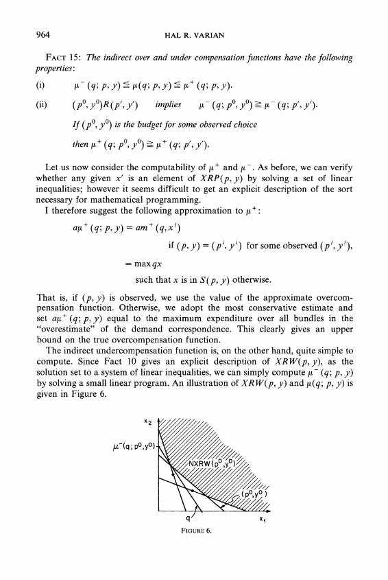
In Section 2 we described the best inner and outer approximations to p(xO).It is natural to define the upper and lower bounds on the compensation function by:

m + ( p , xO) = inf px

such that x is in R p ( x O ) ,

nr - ( p , xO) = inf px

such that x is in NR w ( x O ) .

I refer to these as the overcompensation and the undercompensation functions respectively.

FACT1 1 : Let m and m - be defined as above. Then +

+(ii) x 'Rx implies m + ( p O ,x ') 2 m x ) . ~fx ' R X ~and xJ

is chosen at some price pJ, then m - x ') 2 m - (pO ,x i ) .

PROOF:(i) Follows from Fact 5. (ii) Follows from Fact 7.

Fact 11 shows that: (i) mt ( p , x ) and m - ( p , x ) do bound the compensation function, and (ii) they are themselves utility functions that respect the revealed preference ordering.

960 HAL R. VARIAN

Thus the overcompensation and undercompensation functions provide theoret- ically ideal bounds to the compensation function. The problem with these two functions is that they are rather difficult to compute in practice. Recall that Fact 4 gave us a way to verify whether any given bundle x was an element of RP(X') or R w ( x O ) .However, I do not currently have any explicit description of these two sets of the sort suitable for mathematical programming techniques. So instead I have proceeded by defining two approximations to the overcompensa- tion and undercompensation functions. These two approximations do provide bounds, but they are just not the theoretically tightest bounds. We turn now to a description of these approximations.

Let us define the convex, monotonic hull of { x i: x i R x O ) :

c M ( x O )= interior of convex hull of { x : x 2 x i , x i R x O } .

FACT 12: RP(X') > c M ( x O )for all xO.

PROOF: Let x be a point in c M ( x O )and let p be any price vector that supports x . Then I claim px > px i for some x'RxO.For if not, p would separate x from CM(X'), a contradiction. Since xRxi , xiRxO we have that x is in R p ( x O ) .

Then we can define the approximate overcompensation function by:

am + ( p , xO) = inf px

such that x is in CM(X' ) .

Since c M ( x O )is a convex polytope whose vertices are precisely those xiRxO,we can also describe this minimization problem by:

amt ( p ,xO)= min px i , such that x i ~ x O

Note that this function is quite simple to compute. Nevertheless, this approxi- mate overcompensation function does share some desirable properties with the true overcompensation function.

FACT13:

(1) am + ( p , x ) 2 m + ( p , x ) 2 m ( p , x ) .

(2) xORx implies am + ( p ,xO)2 am+ ( p , x ) .

(3) There exists a convex monotonic preference order >, such that

am + ( p , xO) = m ( p , xO) for all xO.

PROOF: The first two parts are obvious. The third is rather detailed. First we define the order and verify that it works; then we establish its properties.

DEMAND ANALYSIS 96 1

Let x 2 x' if and only if am+ ( p , x ) 2 am+(p , x ' ) . Let us show that the compensation function that goes along with this order is in fact equal to am + ( p , x) .

Let px* solve:

px* = m ( p ,Z ) = min px

such that am+ ( p , x ) 2 am+ ( p , 5)

and let px" solve

px" = am + ( p ,5) = min px ' , such that x 'RZ.

Now x"RF so property (2 )shows that am+ ( p , 2)2 am+ ( p , 5). Hence x" is feasible for the first problem and therefore px* S px".

On the other hand

Next we examine the properties of the preference ordering 2. (a) { x :am+ ( p , x ) 2 k ) is convex. To prove this, we suppose am+ ( p , x ' ) 2 k

and am+ ( p , x" ) 2 k. Let

A = { x ' : x iRx ' } ,

I claim that if x i is in C , then x i is in A U B. For to say x i is in C is to say that there exists a finite sequence such that:

pix' ?pix ' ,

prxr 2 p r x s ,

p'x' 2 p ' ( t x f + ( I - t )x l ' ) .

From the last inequality it is easy to show that either p 'x' 2 p 'x' or p 'x' 2pix", which establishes the claim.

Now, since C cA U B, we have:

k 5 rnin p x 5 rnin px= am+ ( p , tx' + (I - t )x f ' ) .x 1 n A U B x in C

(b) If x' 2 xO,then am ( p , x ' ) L am+ ( p , xO). This follows since { x ' : x 'RX ' )+

c { X I : x i ~ x O j .

Thus am+ x ) is a utility function that bounds the compensation function and the bound is uniformly tight in the sense that there exists a "nice" prefer-ence ordering that actually generates am+ x ) as its compensation function.

HAL R. VARIAN

However it must be pointed out that this ordering typically exhibits regions of satiation, and is in general discontinuous. An example is given in Figure 5. Here all the points in the shaded region are assigned am+ ( p O , x ) = pox'. The approxi- mate overcompensation function increases linearly as one moves out the ray tx , then is constant, and then jumps discontinuously.

We turn now to the problem of computing an approximation to the under- compensation function. The basic trick here is to get an "inner bound" to R w ( x O )by eliminating the nonconvexities shown in Figure 3. We define this inner bound by:

The crucial difference between R w ( x O )and IRW(X') is the requirement that x i # xO. This is made clear in Figure 3. The complement of l R w ( x O ) , NIRW(X') , is then given by:

NIR w ( x O )= { x :p'x > pix' for some x ' # x0 such that xORx'

for all p0 in s ( x O )

This is simply a set of a points defined by a finite number of linear inequalities. Hence there is no problem in computing the "approximate undercompensation function":

am - ( p O ,Z)= inf pox

such that x is in NIRW(X) .

This also shares some desirable features with the true undercompensation func- tion:

DEMAND ANALYSIS

FACT14:

(1) m ( p , x )2 m - ( p , x ) 2 am- ( p , x ) ,

(2) x O ~ x j implies am - ( p ,x O )2 am - ( p ,x j ) .

PROOF: Left to the reader.

Thus am- ( p , x ) bounds the true undercompensation function and it respects the revealed preference ordering, although it does not provide the theoretically ideal bound.

6 . RECOVERABILITY-BOUNDING A SPECIFIC INDIRECT UTILITY FUNCTION

It is natural to extend the results of the last section to indirect utility comparisons. The function one wishes to bound is the indirect income compensa- tion function

where e ( q , u ) is the expenditure function and v ( p , y ) is the indirect utility f ~ n c t i o n . ~An equivalent way to define y ( q ; p, y ) is:

( " (9 ; p, y ) = inf qx

such that x is in X P ( p , y ) = {x :u ( x ) > v ( p ,y ) ) .

Applying the approach of the last section, it appears natural to define the indirect overcompensation function and the indirect undercompensation function by:

~ l + ( q ; p , y ) = i n f q x

such that x is in X R P ( p , y ) ,

p- ( q ; p, y ) = inf qx

such that x is in N X R W ( p , y ) .

Recall that X R P ( p , y ) consists of all bundles revealed preferred to the budget ( p , y ) , and N X R W ( p , y ) consists of all bundles not revealed worse than the budget ( p , y ) ; formal definitions were given in Section 3.

It is by now straightforward to verify the following fact:

5 T l ~ eindirect compensation function was first discussed by McKenzie [19]. It has been extensively treated by Hurwicz and Uzawa [13].

964 HAL R. VARIAN

FACT 15: The indirect over and under compensation functions have the following properties:

(ii) ( p O , y O ) R ( p ' , y ' ) implies p - ( q ; pO, y o ) >= p - ( q ; p', y ') .

If is the budget for some observed choice

then p+ ( 9 ; pO, yo) >= p+ ( q ; p', y ') .

Let us now consider the computability of p+ and p- . As before, we can verify whether any given x' is an element of X R P ( p , y ) by solving a set of linear inequalities; however it seems difficult to get an explicit description of the sort necessary for mathematical programming.

I therefore suggest the following approximation to p+:

ap ' (q ; p, y ) = a m ' ( q , x f ) . .

if ( p , y ) = ( p ' , y ' ) for some observed ( p ' , y ' ) ,

= max qx

such that x is in S ( p , y ) otherwise.

That is, if ( p , y ) is observed, we use the value of the approximate overcom- pensation function. Otherwise, we adopt the most conservative estimate and set up+ ( q ; p, y ) equal to the maximum expenditure over all bundles in the "overestimate" of the demand correspondence. This clearly gives an upper bound on the true overcompensation function.

The indirect undercompensation function is, on the other hand, quite simple to compute. Since Fact 10 gives an explicit description of X R W ( p , y ) , as the solution set to a system of linear inequalities, we can simply compute p- ( q ; p, y ) by solving a small linear program. An illustration of X R W ( p , y ) and p(q; p, y ) is given in Figure 6.

965 DEMAND ANALYSIS

7. SOME APPLICATIONS

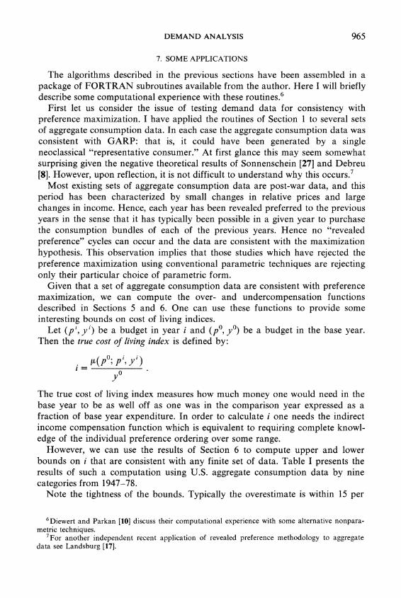
The algorithms described in the previous sections have been assembled in a package of FORTRAN subroutines available from the author. Here I will briefly describe some computational experience with these routine^.^

First let us consider the issue of testing demand data for consistency with preference maximization. I have applied the routines of Section 1 to several sets of aggregate consumption data. In each case the aggregate consumption data was consistent with GARP: that is, it could have been generated by a single neoclassical "representative consumer." At first glance this may seem somewhat surprising given the negative theoretical results of Sonnenschein [27] and Debreu [S]. However, upon reflection, it is not difficult to understand why this occurs.'

Most existing sets of aggregate consumption data are post-war data, and this period has been characterized by small changes in relative prices and large changes in income. Hence, each year has been revealed preferred to the previous years in the sense that it has typically been possible in a given year to purchase the consumption bundles of each of the previous years. Hence no "revealed preference" cycles can occur and the data are consistent with the maximization hypothesis. This observation implies that those studies which have rejected the preference maximization using conventional parametric techniques are rejecting only their particular choice of parametric form.

Given that a set of aggregate consumption data are consistent with preference maximization, we can compute the over- and undercompensation functions described in Sections 5 and 6. One can use these functions to provide some interesting bounds on cost of living indices.

Let ( p ' ,y ' ) be a budget in year i and yo) be a budget in the base year. Then the true cost of living index is defined by:

The true cost of living index measures how much money one would need in the base year to be as well off as one was in the comparison year expressed as a fraction of base year expenditure. In order to calculate i one needs the indirect income compensation function which is equivalent to requiring complete knowl- edge of the individual preference ordering over some range.

However, we can use the results of Section 6 to compute upper and lower bounds on i that are consistent with any finite set of data. Table I presents the results of such a computation using U.S. aggregate consumption data by nine categories from 1947-78.

Note the tightness of the bounds. Typically the overestimate is within 15 per

'Diewert and Parkan [lo] discuss their computational experience with some alternative nonpara- metric techniques.

'For another independent recent application of revealed preference methodology to aggregate data see Landsburg [17].

HAL R. VARIAN

TABLE I UPPERAND LOWERBOUNDON TRUECOSTOF LIVINGINDEX^

(CLASSICAL IN PARENTHESES)BOUNDS

Year Upper Bound Lower Bound

dData are U.S. consumption data by 9 categories from the NBER Time Series Database (Tables 2.3 and 2.4). The goods are motor vehicles, furniture, other durables, food, clothing, gasol~ne and oil, housing, transportation, and other services.

cent of the underestimate which allows for a fairly tight estimate of the true cost of living. However, the accuracy of the table is slightly misleading in the following sense.

Given only the information contained in the two observations yo) and ( p ' ,y ' ) it is possible to construct the classical bounds depicted in Figure 7. Improvements in these bounds are possible only when some budget set from another sample observation intersects the budget set given by ( p ' ,y ' ) as in Figure 8.

Given the nature of the data, these intersections are quite rare, and in fact only occur for two years 1974 and 1975. Again, the lack of variation in the price data

DEMAND ANALYSIS

Improved

limits the power of these methods in this case. However, the techniques proposed here do provide an improvement on the classical bounds when sufficient varia- tion in price data is present.

8. SUMMARY

We have shown how the nonparametric techniques of revealed preference analysis can be used to: (1) test a finite amount of data for consistency with preference maximization model; (2) construct a nicely behaved utility function capable sf rationalizing a finite amount of demand data; (3) compare previously unobserved consumption bundles and budgets with respect to their ordinal rankings; (4) compute cardinal bounds on the direct and indirect compensation functions; and (5) compute estimates of the direct and indirect demand corre- spondence consistent with previously observed demand data.

University of Michigan

Manuscript received August, 1980; final revision received August I, 1981.

HAL R. VARIAN

APPENDIX I: A PROOF OF AFRIAT'S THEOREM

In this appendix we give a proof of Afriat's theorem. The proof we give is based on earlier proofs by Afriat [4] and Diewert [9], but is somewhat more constructive. In fact we will exhibit an algorithm which will actually compute a utility function which rationalizes any given finite amount of data. It turns out that it is convenient to first describe the algorithm to do this computation and then verify that it works in the course of the proof of Afriat's theorem.

The algorithm that we describe below makes use of a subroutine which calculates a maximal element of a finite set with respect to some binary relation.

Let us recall the following definition.

DEFINITION:An element x m of a set S is maximal with respect to a binary relation B if xiBx'" implies x "Bx'.

If x'" is a maximal element then either there is nothing that is ranked ahead of it or the only things that are "ahead" of it are things that are indifferent to it.

If we have a finite set with a reflexive and transitive binary relation then there is always at least one maximal element; the following algorithm shows us how to find it. (See Sen [26, p. 111.)

ALGORITHM2: Finding a maximal element. Input: a reflexive and transitive binary relation B defined on a finite set S = (x ' , . . . ,x n )

indexed by I = (1 , . . . , n). Output: an index m where x'Bxm implies x'"Bxl. 1. Set m = 1, bO= x ' . 2. For each i = 1 , . . . , n, if x ' B ~ " ' set b' = x i , and m = i. Otherwise set b ' = b l - ' .

We will let max(1) be a routine that performs Algorithm 2; that is, given a set S indexed by I , max(1) returns the index of a maximal element in S .

It is perhaps not immediately obvious that Algorithm 2 works. Hence we provide the following proof.

FACT 15: The output of Algorithm 2 is the index of a maximal element of S .

PROOF: First we note that by the transitivity and reflexivity of B, bnBbJ for all j = 0, . . . , n. Also note that x m = b ".

Now suppose we are given some x'Bxm; i.e. x'Bbn. We must show that b"Bxl. First we observe that since x'Bbn, and bnBb'- l , then x ' B b ' I . Line 2 of the algorithm then implies b ' = x i . But then b"Bbl, b' = x ' gives h"Bxl as required.

We note that the revealed preference relation R is transitive and reflexive, so Algorithm 2 will therefore correctly compute a maximal element. We can now present an algorithm which calculates numbers that satisfy the Afriat inequalities:

ALGORITHM Constructing the Afriat numbers. 3: Input: A set of demand observations (pi,x') , i = 1, . . . , n, and the revealed preference relation R

that satisfy CARP. Output: A set of numbers Ui, A ' > 0, i = 1, . . . , n, that satisfy the Afriat inequalities. 1. I = ( l , . . . , n ] , B = 0 . 2. Let m = max(1). 3. Set E = ( i in I : xiRxm). If B = 0 , set Urn = A m = 1 and go to 6. Otherwise go to 4. 4. Set Urn = min,E,minJ,Bmin( UJ + A$j(xi - xJ), UJ). 5. Set A m = max,,,max,EBmax((UJ - Um)/pi(xJ - x'), 1). 6. Set U' = Urn,A ' = A m for all i E E. 7. Set I = I \ E , B = B U E. If I = 0 , stop. Otherwise, go to 2.

It is not at all obvious that Algorithm 3 does in fact compute numbers that satisfy the Afriat inequalities; however that fact will be verified in the proof of Afriat's theorem.

DEMAND ANALYSIS

AFRIAT'S THEOREM: The following conditions are equivalent: ( 1 ) There exists a nonsatiated utility function that rationalizes the data. (2) The data satisjes GARP: if xlRxJ , then pJxJ 5 pJxl. (3) There exist numbers U', X' > 0 such that U' 5 UJ+ XJpJ(x' - x J ) for i, j = 1, . . . ,n. (4) There exists a nonsatiated, continuous, concave, monotonic utility function that rationalizes the

data.

PROOF:(1)*(2). Let u ( x ) rationalize the data. If pix' 2 p ' x J then u ( x i )2 u ( x J )by definition so that X'ROXJimplies u ( x i )2 u (xJ ) .If pix' >p'xJ so that xipOxJ,then I claim that u ( x i )> u(x j ) . If not, then u ( x l )= u(xJ ) .But by local nonsatiation there is then an i such that p'x' >p'2 and u(;) > u ( x i ) . But then u ( x ) could not rationalize the data point ( p ' , x i ) . Hence ~ ' P ' X J implies u ( x l )> u ( x J ) ,and GARP follows.

(2)*(3). In order to prove this we need to verify that Algorithm 3 works; i.e., that the numbers it calculates do indeed satisfy the Afriat inequalities.

At each pass through the algorithm a set of indices of "equivalent" elements, E , is removed from I and added to B, a set of indices of "better" elements. We will show that after step 6 is executed, the U's and the A's at that stage satisfy the Afriat inequalities for all the U's and X's calculated up to that point. That is, we will verify the following three statements:

(a) U' 5 UJ+ X-'pJ(xi- x J ) for all j in B and all i in E,

(b) UJ5 U' + h 'p ' (xJ- x ' ) for all j in B and all i in E,

(c) U' 5 UJ+ XJpJ(xl- x J ) for all i and j in E.

Proof of ( a ) : By step 4 of the algorithm:

U' = Urn5 UJ+ XJpJ(xi- x J ) for all j in B and all i in E.

Proof of (b): First note that when the algorithm correctly executes statement 5, pi(xJ - x i )> 0, for all j in B. If not, xlRxJ for some j in B. But then i would have been moved into B before j was moved into B.

Hence, the division is well defined and

A' = A" 2 UJ- U' for all j in B and all i in E . p Z ( x J- x i )

Cross multiplying:

X$'(xi - x i ) 2 UJ- U' for a l l j in B and all i in E

which proves (b). Proof of (c ) : First note that i, j in E implies p J ( x i- x i ) 2 0. If not X J P ' ~ ' ,giving a violation of

GARP. Now for all i and j in E :

U ' = U J and X J = X m > O

(3)*(4). We define the function U ( x )by

U ( x )= min { U' + X'pl(x - x ' ) ) . I

It is clear from the definition that this piecewise linear function has the stated properties. Hence we only need to verify that it rationalizes the data.

970 HAL R.VARIAN

First we note that U(x') = U' for all i = 1, . . . , n. For suppose the minimum is attained at x m ; then

since h'"p(xx' - x ' ) = 0. But if this inequality were ever strict we would violate one of the Afriat inequalities.

Now suppose we are given some x such that pJxJ 2 p J x . We must show that U(xJ) 2 U(x). This follows directly from the following set of inequalities:

U(x) = min { U' + X'pi(x - x i ) ) I

since XJpJ(x - xJ) 5 0. (4)* (I). This is obvious.

It is worthwhile giving a somewhat more heuristic argument for Afriat's Theorem, which more directly exhibits the meaning of the Afriat inequalities. Suppose that we have a differentiable concave utility function that rationalizes some data ( p l , x ' ) , i = 1, . . . ,n. Then concavity implies

and utility maximization implies

Putting these together we see that the Afriat conditions are a necessary condition for utility maximization in this differentiable framework. To motivate the sufficiency result we simply note that by concavity we have n overestimates of the utility at some point x since

U(X)5 ~ ( x ' )+ X'pl(x - x ' ) for i = 1, . . . ,n.

Hence the minimum of the right hand side over all observation i-the lower envelope-should give us a reasonable measure of the utility of x.

This interpretation of the U"s as utility levels and the hi's as the marginal utilities of income was first suggested by Afriat [I] and further elucidated by Diewert and Parkan [lo]. Varian [29, 301, has used this sort of argument to derive finite necessary and sufficient conditions for a number of specializations of the utility maximization model.

Finally we give a proof of one last fact concerning Afriat's construction that was stated without proof at one point in the text. If x ' is not revealed preferred to xJ, then it is intuitively plausible that there is a nice utility function that rationalizes the data for which u(xJ) 2 u(xi). This is verified in the next statement.

FACT 16: If not x'RxJ, then there is a nonsatiated, continuous, concave, monotonic utility function that rationalizes the data for which u(xJ) 2 u(xl).

PROOF: Simply ensure that, max(I) returns the index j before the index i. Line 4 of Algorithm 3 then implies that u(xJ) 2 u(xl) .

APPENDIX 11: COMPUTING CLOSURETHE TRANSITIVE

The following discussion concerning the computation of the transitive closure of a relation is taken from Aho and Ullman [6], which in turn is based on Warshall [31]. Their results are very slightly generalized in a way that is useful in some other applications (Varian [29]).

DEMAND ANALYSIS

Let M be an n by n matrix representing a binary relation; i.e. my = 1 if X'R'XJ and m,, = 0 otherwise. We can also think of M as representing a directed graph as in Figure 9: there is an arrow from vertex i to vertex j if and only if my = 1. It is this interpretation that gives rise-somewhat indirectly-to Warshall's algorithm.

Suppose now that we have an arbitrary directed graph and some associated cost function c,, where c,, P 0 measures the cost of transporting one unit of a good directly from vertex i to vertex j. If vertex i and vertex j are not directly connected c,, is by definition infinite. Now although the cost of moving i toj directly is given by c,,, the cheapest cost of moving i to j may be much less. Warshall's algorithm is concerned with calculating the least cost of moving from any vertex to any other vertex. We denote the magnitude of this least cost by T,,.

I claim that if we can solve this "least cost problem" we can easily solve the "transitive closure" problem. We just create a cost matrix C where

1 i f m , , = I , c,, = { cc if m,, = 0.

Now we run C through Warshall's algorithm to compute the least cost matrix (Z,,): Then if FU = I < m we know that there is some path of length 1 that connects vertex i with vertex J. Hence a method to solve the least cost problem gives us a method to solve the transitive closure problem.

ALGORITHM4: Minimum cost of paths in a graph. Input: c,, = cost of moving from node i to node j ; c, 2 0. Output: zY = minimum cost of moving from node i to node j . (1)Set k = 1. (2)For all i and j,if c,, 2 c,, + ckJ set c,, = c,, + ckJ. (3) If k < n, let k = k + 1 and go to 2. If k = n, set z, = c,, for all i and j.

It is not at all obvious that Algorithm 4 does indeed compute the minimum cost of moving from i toj for all i and j.But the following argument shows that it works.

FACT 17: Let (i,I , . . . , m , j) be a path from i to j. Then T , 5 c,, + . . . + cmJ.

PROOF:Consider the algorithm when it has completed step (2).We will show that c,, is the cost of the cheapest path from i to j that passes through no intermediate vertex with index greater than k. This is certainly true for k = 1, and we suppose it to be true for k - 1.

Let (I,I , . . . , m , j) be a path from i to j that passes through no intermediate vertex with index greater than k. If it does not pass through vertex k we are done. If it does pass through k, we can suppose it only passes through once, since removing a cycle cannot increase the cost. By the induction hypothesis c,, is the cheapest path from i to k with no intermediate vertex greater than k - 1 and similarly for ckJ.Since step (2)of the algorithm ensures c,, 5 c,, + cg , we are done.

Note that step (2)of the algorithm will be executed n3 times; thus we can compute the transitive closure of a relation in n3 computer additions and comparisons. Of course, if we are using Warshall's algorithm only to compute the transitive closure of a relation we can improve a bit on that bound. Consider for example the following FORTRAN subroutine which computes the transitive closure of a relation represented by the matrix M .

972 H A L R. V A R I A N

ALGORITHM5: Computing the transitive closure. Input: M ( I , J ) = 1 if p'x' 2 p 1 x J , 0 otherwise. N = number o f observations; nobs = maximum

number o f observations. Output: M ( I , J ) = 1 i f x 'RxJ , 0 otherwise.

SUBROUTINE T C L S R ( M , N ) DIMENSION M(nobs, nobs) D O 3 0 K = l , N D O 2 0 I = l , N DO l O J = l , N IF ( M ( I , K ) .EQ. 0 .OR. M ( K , J ) .EQ. 0 ) G O T O 10 M ( I , J ) = 1

10 CONTINUE 20 CONTINUE 30 CONTINUE

RETURN E N D

This clearly computes the transitive closure by a straightforward modification o f the argument given in Fact 17.

REFERENCES

[I] AFRIAT, S.: "The Construction o f a Utility Function from Expenditure Data," International Economic Review, 8(1967), 67-77.

[2] --: "The Theory o f International Comparison o f Real Income and Prices," International Comparisons of Prices and Output, ed, by D. J . Daly. New Y o r k : National Bureau o f Economic Research, 1972.

[31 -: "On a System o f Inequalities on Demand Analysis: A n Extension o f the Classical Method," International Economic Review, 14(1973), 460-472.

[4] --: The Combinatorial Theory of Demand. London: Input-Output Publishing Company, 1976.

[51 --: The Price Index. London: Cambridge University Press, 1977. [6] AHO, A , , AND J . ULLMAN:The Theory of Parsing, Translation, and Compiling, Volume I : Parsing.

Englewood Cli f fs , New Jersey: Prentice-Hall, Inc., 1972. [7] DOBELL, A , : " A Comment on A . Y . C. Koo's ' A n Empirical Test o f Revealed Preference

Theory'," Econometrica, 33(1965), 451-455. [8] DEBREU,G.: "Excess Demand Functions," Journal of Mathematical Economics, 1(1974), 15-22. [9] DIEWERT,E.: "Afriat and Revealed Preference Theory," Review of Economic Studies, 40(1973),

419-426. [lo] DIEWERT,E., AND C . PARKAN: "Test for Consistency o f Consumer Data and Nonparametric

Index Numbers," University o f British Columbia, W.P. 78-27, 1978. [ l l ] HANOCH, G., AND M. ROTHSCHILD: the Assumptions o f Production "Testing Theory: A

Nonparametric Approach," Journal of Political Economy, 80(1972), 256-275. [12] HOUTHAKKER, "Revealed Preference and the Utility Function," Economica, 17(1950),H.:

159-174. [13] HURWICZ, L., AND H. UZAWA: "On the Integrability o f Demand Functions," in Preference

Utility and Demand, ed. by J . S. Chipman, et al. New York: Harcourt, Brace, Jovanovich, 1971.

[14] Koo, A.: " A n Empirical Test o f Revealed Preference Theory," Econometrica, 31(1963), 646-664. [Is] -: "Reply," Econometrica, 32(1965), 456-458. [I61 -: "Revealed Preference-A Structural Analysis," Econometrica, 39(1971), 89-98. [17] LANDSBURG,S.: "Taste Change in the United Kingdom 1900-1955," Journal of Political

Economy, 89(1981), 92-104. [18] LITTLE,J . : "Indirect Preferences," Journal of Economic Theory, 20(1979), 182-193. [19] MCKENZIE,L.: "Demand Theory Without a Utility Index," Review of Economic Studies,

24(1956), 185-189. [20] MUNROE,I.: "Efficient Determination o f the Transitive Closure o f a Directed Graph," Informa-

tion Processing Letters, 1(1971), 56-58.

DEMAND ANALYSIS

[21] RICHTER, M.: "Revealed Preference Theory," Econometrica, 34(1966), 635-645. [22] -: "Duality and Rationality," Journal of Economic Theory, 20(1979), 13 1-18 1. [23] SAKAI, Y.: "Revealed Favorability, Indirect Utility, and Direct Utility," Journal of Economic

Theory, 113-129. [24] SAMUELSON,P.: "Consumption Theory in Terms of Revealed Preference," Economica, 15(1948),

243-253. PSI -: "Complementarity," Journal of Economic Literature, 7(1979), 1255-1289. [26] SEN, A.: Collective Choice and Social Welfare. San Francisco: Holden-Day, 1970. [27] SONNENSCHEIN,H.: "Do Walras' Identity and Continuity Characterize the Class of Community

Excess Demand Functions?" Journal of Economic Theory, 6(1973), 345-354. [28] UEBE,G.: "A Note on Anthony Y. C. Koo, 'Revealed Preference-A Structural Analysis',"

Econometrica, 40(1972), 771-772. [29] VARIAN,H.: "Nonparametric Tests of Consumer Behavior," University of Michigan, CREST

Working Paper, 1980; forthcoming in Review of Economic Studies. P O I --: "Nonparametric Tests of Models of Investment Behavior," University of Michigan,

CREST Working Paper, 198 1. [31] WARSHALL,S.: "A Theorem on Boolean Matrices," Journal of the American Association of

Computing Machinery, 9(1962), 11-12.

You have printed the following article:

The Nonparametric Approach to Demand AnalysisHal R. VarianEconometrica, Vol. 50, No. 4. (Jul., 1982), pp. 945-973.Stable URL:

http://links.jstor.org/sici?sici=0012-9682%28198207%2950%3A4%3C945%3ATNATDA%3E2.0.CO%3B2-O

This article references the following linked citations. If you are trying to access articles from anoff-campus location, you may be required to first logon via your library web site to access JSTOR. Pleasevisit your library's website or contact a librarian to learn about options for remote access to JSTOR.

[Footnotes]

5 Demand Theory Without a Utility IndexLionel McKenzieThe Review of Economic Studies, Vol. 24, No. 3. (Jun., 1957), pp. 185-189.Stable URL:

http://links.jstor.org/sici?sici=0034-6527%28195706%2924%3A3%3C185%3ADTWAUI%3E2.0.CO%3B2-O

7 Taste Change in the United Kingdom, 1900-1955Steven E. LandsburgThe Journal of Political Economy, Vol. 89, No. 1. (Feb., 1981), pp. 92-104.Stable URL:

http://links.jstor.org/sici?sici=0022-3808%28198102%2989%3A1%3C92%3ATCITUK%3E2.0.CO%3B2-9

References

1 The Construction of Utility Functions from Expenditure DataS. N. AfriatInternational Economic Review, Vol. 8, No. 1. (Feb., 1967), pp. 67-77.Stable URL:

http://links.jstor.org/sici?sici=0020-6598%28196702%298%3A1%3C67%3ATCOUFF%3E2.0.CO%3B2-K

http://www.jstor.org

LINKED CITATIONS- Page 1 of 4 -

NOTE: The reference numbering from the original has been maintained in this citation list.

3 On a System of Inequalities in Demand Analysis: An Extension of the Classical MethodS. N. AfriatInternational Economic Review, Vol. 14, No. 2. (Jun., 1973), pp. 460-472.Stable URL:

http://links.jstor.org/sici?sici=0020-6598%28197306%2914%3A2%3C460%3AOASOII%3E2.0.CO%3B2-K

7 A Comment on A. Y. C. Koo's "An Empirical Test of Revealed Preference Theory"A. R. DobellEconometrica, Vol. 33, No. 2. (Apr., 1965), pp. 451-455.Stable URL:

http://links.jstor.org/sici?sici=0012-9682%28196504%2933%3A2%3C451%3AACOAYC%3E2.0.CO%3B2-V

9 Afriat and Revealed Preference TheoryW. E. DiewertThe Review of Economic Studies, Vol. 40, No. 3. (Jul., 1973), pp. 419-425.Stable URL:

http://links.jstor.org/sici?sici=0034-6527%28197307%2940%3A3%3C419%3AAARPT%3E2.0.CO%3B2-9

11 Testing the Assumptions of Production Theory: A Nonparametric ApproachGiora Hanoch; Michael RothschildThe Journal of Political Economy, Vol. 80, No. 2. (Mar. - Apr., 1972), pp. 256-275.Stable URL:

http://links.jstor.org/sici?sici=0022-3808%28197203%2F04%2980%3A2%3C256%3ATTAOPT%3E2.0.CO%3B2-8

12 Revealed Preference and the Utility FunctionH. S. HouthakkerEconomica, New Series, Vol. 17, No. 66. (May, 1950), pp. 159-174.Stable URL:

http://links.jstor.org/sici?sici=0013-0427%28195005%292%3A17%3A66%3C159%3ARPATUF%3E2.0.CO%3B2-J

14 An Empirical Test of Revealed Preference TheoryAnthony Y. C. KooEconometrica, Vol. 31, No. 4. (Oct., 1963), pp. 646-664.Stable URL:

http://links.jstor.org/sici?sici=0012-9682%28196310%2931%3A4%3C646%3AAETORP%3E2.0.CO%3B2-X

http://www.jstor.org

LINKED CITATIONS- Page 2 of 4 -

NOTE: The reference numbering from the original has been maintained in this citation list.

15 A Comment on A. Y. C. Koo's "An Empirical Test of Revealed Preference Theory": ReplyAnthony Y. C. KooEconometrica, Vol. 33, No. 2. (Apr., 1965), pp. 456-458.Stable URL:

http://links.jstor.org/sici?sici=0012-9682%28196504%2933%3A2%3C456%3AACOAYC%3E2.0.CO%3B2-Q

16 Revealed Preference--A Structural AnalysisAnthony Y. C. KooEconometrica, Vol. 39, No. 1. (Jan., 1971), pp. 89-97.Stable URL:

http://links.jstor.org/sici?sici=0012-9682%28197101%2939%3A1%3C89%3ARPSA%3E2.0.CO%3B2-G

17 Taste Change in the United Kingdom, 1900-1955Steven E. LandsburgThe Journal of Political Economy, Vol. 89, No. 1. (Feb., 1981), pp. 92-104.Stable URL:

http://links.jstor.org/sici?sici=0022-3808%28198102%2989%3A1%3C92%3ATCITUK%3E2.0.CO%3B2-9

19 Demand Theory Without a Utility IndexLionel McKenzieThe Review of Economic Studies, Vol. 24, No. 3. (Jun., 1957), pp. 185-189.Stable URL:

http://links.jstor.org/sici?sici=0034-6527%28195706%2924%3A3%3C185%3ADTWAUI%3E2.0.CO%3B2-O

21 Revealed Preference TheoryMarcel K. RichterEconometrica, Vol. 34, No. 3. (Jul., 1966), pp. 635-645.Stable URL:

http://links.jstor.org/sici?sici=0012-9682%28196607%2934%3A3%3C635%3ARPT%3E2.0.CO%3B2-G

24 Consumption Theory in Terms of Revealed PreferencePaul A. SamuelsonEconomica, New Series, Vol. 15, No. 60. (Nov., 1948), pp. 243-253.Stable URL:

http://links.jstor.org/sici?sici=0013-0427%28194811%292%3A15%3A60%3C243%3ACTITOR%3E2.0.CO%3B2-0

http://www.jstor.org

LINKED CITATIONS- Page 3 of 4 -

NOTE: The reference numbering from the original has been maintained in this citation list.

28 A Note on Anthony Y. C. Koo, "Revealed Preference--A Structural Analysis"Goetz UebeEconometrica, Vol. 40, No. 4. (Jul., 1972), p. 771.Stable URL:

http://links.jstor.org/sici?sici=0012-9682%28197207%2940%3A4%3C771%3AANOAYC%3E2.0.CO%3B2-N

http://www.jstor.org

LINKED CITATIONS- Page 4 of 4 -

NOTE: The reference numbering from the original has been maintained in this citation list.