Discussion PaperCentral Bureau of Statistics, P.B. 8131 Dep, 0033 Oslo 1, Norway

No. 32 _ 28. March 1988

THE OIL MARKET AS AN

OLIGOPOLY

BY

Kjell Berger, Michael Hoel,

Steinar Holden and Øystein Olsen

1Abstract

This paper treats the oil market as an oligopoly with a competitive fringe.The oligopoly is assumed to consist of Egypt, Oman, Mexico, Malaysia andNorway plus all OPEC members. The remaining oil producing countries areincluded in a fringe which by assumption takes the oil price development asexogenously given. Outcomes with varying degrees of collusion within theoligopoly are specified. Intermediate cases are also studied, such as completeor partial cooperation within OPEC, but no cooperation between OPEC andany other countries in the oligopoly. The model is implemented in the PC-based MODLER software, and empirical results from the simulations on thedifferent model versions are presented.

Not to be quoted without permission from author(s). Comments welcome.

THE OIL MARKET AS AN OLIGOPOLY

Kjell Berger, Michael Hoel, Steinar Holden and . Øystein Olsen *

Contents

1 Introduction

3

2 Restricting the theoretical framework

4

3 The demand for oil

5

4 Oil supply from countries outside the oligopoly

5 Demand and cost functions of the oligopoly

6 Different behavioural models for the oligopoly 96.1 The oil market as a Cournot oligopobr . . . . . . • • • • • • • . • . 96.2 Collusion in the oil oligopoly . . . . . . • • • .• • • • • • • • • • . 9

6.3 Proportionate adjustment of production levels . • . • • •

. . . . . . 10

. 7 Empirical results 117.1 Oligopoly . . . . • . • . • • • • • • • • • • • • • . . . : . . . . . . . 127.2 OPEC cartel with side payments • . . . . . . • • • 0 • • • • • • • • 147.3 OPEC cartel with proportionate reduction of supplies . . . . • . . 15

7.4 A cartel model includin g all 18 oil producers . . . . . • • • . . . • 16

8 Concluding remarks 16

9 References 17

•Michael Hod and Steinar Holden ari at the Department of Economics, University of Oslo.Kjell Berger and Øystein Olsen are with the Group of Petroleumeconomic Research, CentralBureau of Statistics

1 Introduction

The future price development for oil will depend on to what extent the OPECmembers are able to coordinate their production decisions, and to what extentOPEC succeeds in cooperating with other major oil producers. Many countriesboth inside and outside OPEC will suffer through large reductions in incomes bya fail in the oil price as a result of breakdown of OPEC. This obviously formsthe background for the fact that some countries outside the organization havefound it beneficial to negotiate with OPEC it order to support OPEC's controlover the market. For each agent in the market this kind of agreement must beweighted against the benefits of being a "free rider" in the market. The questionof benefits from cooperation with OPEC from the point of view of Mexico andNorway is- discussed in Berger, Bjerkholt and Olsen (1987). This analysis used asimple partial equilibrium model (WOM) for the international oil market as itspoint of departure, and the issue of cooperation was then approached by differentassumptions of exogenous oil supplies from different regions. Thus, no formalbehavioural relations on the supply side of the oil market were underlying thesesimulations. Even though it may be questioned whether a formal cartel modelis suited for fitting the obviously complex relations in the international crude oilmarket, we still believe that a more formal analysis is useful as a supplement ofunderstanding present and future development in the market.

This paper treats the oil market as an oligopoly with a competitive fringe.Consistent with the reasoning in Berger et al. (op. cit) we assume that Egypt,Oman, Mexico, Malaysia and Norway are the oil producers outside OPEC whichare most likely to cooperate with OPEC. The oligopoly is thus rammed to consistof these countries plus all OPEC members. The remaining oil producing countriesare included in a fringe which by assumption takes the oil price developmentas exogenously given. We consider outcomes with varying degrees of collusionwithin the oligopoly. One extreme case is characterized by a complete breakdownof cooperation within the oligopoly. In this case we assume that the Cournotsolution is the market outcome. The opposite extreme is the situation where allcountries in the oligopoly cbordinate their production decisions so that the totalprofit of the oligopoly is maximized. We also consider intermediate ca lms, suchas complete or partial cooperation within OPEC, but no cooperation betweenOPEC and any other countries in the oligopoly.

The net demand for crude oil which the oligopoly is facing is roughly consis-tent with demand and supply relations in the WOM model. The procedure forcalibrating net oil demand in the present framework will be outlined below.

The rest of the paper is organized as follows. In the following section limi-tations of the theoretical framework will be briefly discussed. Section 3 and 4

2

describe our assumptions about totil demand for oil and the supply of oil from thecompetitive fringe. Section 5 briefly surveys the cost functions of the oligopolymembers. In section 6 we present the specific theoretical models that are im-plemented. and tested empirically, comprising both the pure Cournot solutionand cases with varying degrees og collusion between oligopoly members. Epiricalresults from simulations on the different model versions are given in section 7.Finally, some concluding comments are given in section 8.

2 Restricting the theoretical framework

Throughout this paper we have ignored the fact that oil is a depletable resource.There are two reaions for doing this. The fast reason is that we want the modelto be as simple and easy to use as possible. It is well known from the literature(see e.g. Newbery (1981)) on exhaustible resources that it is quite difficult toderive numerical solutions to several of the possible solution concepts in oligopolymodels of exhaustible resources. Our model framework is intended to be a tool forplanners in Norwegian government agencies, oil companies etc. For this purposethe structure of the model must be reasonably simple, and its mechanisms mustbe well understood by the users.

A second reason for ignoring the fact that oil is depletable is that all Hotellingtypes of models force us to specify the appropriate interest rate for each country.It is not obvious that the countries use interest rates-from international financialmarkets in their considerations about how much oil they should extract at differ-ent points of time. Moreover, international interest rates may depend on OPECbehaviour. This makes the intertemporal decision problems of OPEC-countrieseven more complex than they are with exogenous interest rate (see e.g. Hoel(1981)). By simply ignoring the depletion issue, from a strictly formal point ofview we obtain results corresponding to producers having an infinite interest rate.Since high interest rates tend to increase extraction and reduce prices under allmarket structures, the fact that we ignore the exhaustibility of oil implies thatwe tend to overestimate production and underestimate price in our model.

We shall also disregard intertemporal aspects of demand and supply func-tions. In reality, price changes only gradually affect demand and fringe supply.This meant; that price changes will only gradually affect the residual demandfacing the oligopoly. Our model uses long run demand and supply functions,i.e. we restrict ourselves to long run equilibria. This also means that we as-sume that participants in the oligopoly only consider long run consequences ofalternative production levels. If oligopoly members have a positive interest rate,rational behaviour implies that both short and long run effects will be considered

3

when agents choose their optimal production strategy (see e.g. Hnyilkza andPindyc.k (1976)). By completely ignoring short run considerations, we thus tendto overestimate production and underestimate price in our model, since shortrun elasticities are smaller than long run elasticities (in absolute value). Ourpredicted prices may thus be biased downwards due both to our ignoring of thefact that oil is depletable and because we only consider long run elasticities inour description of the behaviour of the oligopoly members.

However, a couple of other features of the model specification tend to over-estimate prices, especially in the long run. Firstly, in the model simulationscapacities of oligopoly members are kept constant, pushing up marginal costs asdemand and production pow. Secondly, in the calculations we have disregardedfrom the influences of increased substitutability in the oil market, represented inits purest form of the presence of a back-stop technology. Altogether, one maysay that our model introduces a negative bias on prices in the short to mediumrun, but tend to overestimate prices in the long run.

In the present version of our model, capacity limits of all oligopoly membersare exogenous. For a long run analysis this is clearly unsatisfactory. In a laterversion of our model we plan to endogenize production capacities. The simplestway of doing this is to use long run cost functions, which include the cost ofcapacity expansion.. An alternative procedure is to model the oligopoly marketas a two stage game. In the first stage, the capacity of each country is determinedas a Nash equilibrium of a non-cooperative game. The second stage of the gamemay be modeled in a similar way as will be described in the following, i.e. withexogenous capacity. The capacity chosen in the first stage will affect the outcomein the second stage and consequently the payoff to each player. The relationshsigbetween capacities and payoffs will depend on the degree of collusion in the secondstage of the game. One way of modeling the capacity decisions in the first stageis to assume that the players have subjective probability distributions over thedifferent market structures which may arise in the second stage of the game.

However, as mentioned above, so far we treat production capacities as exoge-nous in the model, and we now proceed to explain this framework.

3 The demand for oil

Total world oil demand (outside the East Bloc and China) in the oligopoly modelis specified as

D = D(P, Zd) (1)

P is the oil price in (real) dollars. Zd is a vector of exogenous factors, in-

4

chiding income levels in different countries, real exchange rates, and prices ofother energy sources. As mentioned in the introduction, (1) is derived from theWOM model. More specifically, D is the sum of the oil demand of three regionsin WOM, namely USA, the rest of OECD, and the LDC's. In each region i(i = USA, OECD, LDC) oil demand is given by

= AiXtP:iQr (2)

where Xi is GNP, Pi is the real price of oil products (in local currency), Qi isan index representing the real price of alternative energy, and Ai is an exogenousvariable expressing the effects of all other exogenous factors, including a possibletime trend. The oil price in local currency is

Pi = (IMP + (1 — 'MCA (3)

where ri is the real exchange rate (rusA = 1), Ci is the cost (in local cus-rency) of transportation, refining, distribution and storage of oil products, andTi represents the tax wedge due to indirect taxes on oil products.

Notice that there are no time lags in our demand function (2), as opposed tothe WOM model wher there is a Koyck lag structure on price responses. Thismeans that the demand elasticities A, ei and ;hi in (2) must be interpreted aslong run elasticities. We have used the following elasticities in our analysis:

USA OECD LDC 'GNP elasticity (/3i) 0.70 0.80 4 1.00 4

Oil price elasticity (4) -0.93 -0.91 -0.37Price elasticity ofalternative energy (p,i ) 0.20 0.37 0.40

Since the variables Ai, Xi, Qi, r, C, Ti, are exogenous in our analysis, wemay summarize (2) and (3) and derive D = Di , yielding (1).

4' Oil supply from countries outside the oligopoly

Total world supply from the countries outside the oligopoly (including nt exportsfrom the East Bloc) is specified as

S = S(P, Z.) (4)

5

In our specification, the only exogenous factor in the supply function (Le. inZ. in (4)) is a time trend. The time trend is included to represent a graduallydeclining supply, for a constant oil price, due to depletion.

More specifically, (4) can be thought of as derived from a supply function

(t) = S (P (t) , R(t)) (5)where R(t) is cumulative extraction. (In order to avoid any misunderstanding,

we include the time dependency of the variables in this part of our analysis.) Weassume that asiap› 0 and asiaR< O.

The development of R(r) is given by

it(r) = S (P (r) , R(r)) (6)

If the time path of P(r) for r E [0, ti was known, R(t) would follow from thedifferential equation (6) and the initial value .R4 (= R(0), with t = 0 being thebase year) of cumulative extraction.

Our model is designed to give a description of the oil market at some futuredate, e.g. year 2000 or 2010. The model - is not intended to give a full intertem-poral description of possible oil price developments. In order to motivate (4) wemay thus just as well assume a certain structure of the oil price developmentfrom the base year 0 to our prediction year, in which case P(r) follows from Po,P(t) and t. An example of this is an oil price path with a constant growth rate,yielding P (r) = Po(P (t) I For . But if P(r) is completely determined by Po P (t)and r, so is R(t) — Re (cf. the discussion above). We may therefore write

R(t) = 0(P(t),Po,t,R0)

(7)

Inserting (7) into (5) gives

= (P, t(P , Po, t Ron

or

S = S (P,t) (8)

where we have omitted Po and Ro, since they are fixed throughout our anal-

The resulting supply function (8) is identical to (5), except that the generalvector of exogenous factors in (5) is substituted by the specific time trend in (8).

Our numerical model is towed on the following specification of (8)

S=B•re't

(9)

where B is a constant term. This supply equation is calibrated in the followingway: In the WOM model a submodel is specified for the group of producersoutside OPEC. In this submodel oil production from these countries are related tovarious concepts of oil reserves, and exploration and extraction of these reservesare depending on the (expected) oil price. For given assumptions of the oilprice and other independent variables this submodel is simulated a number ofyears ahead (until 2000), yielding non- OPEC supply for varying combinationsof explanatory variables. The resulting set of "synthetic" data are then used forestimating the simpler supply behaviour in the oligopoly model represented by(9). Given that we "believe" in the supply structure in the WOM model, thismay seem as a reasonable procedure.

The supply elasticity o is by this procedure estimated to 0.117 , and the timetrend parameter obtained is -0.008.

5 Demand and cost functions of the oligopoly

The participants of the oligopoly are all of the OPEC countries plus Egypt,Oman, Mexico, Malaysia and Norway. The remainin' g oil producing countriesare included in a competitive fringe.

The residual demand facing the oligopoly is

E = = D(P, Zd) Z.) (10)

Z represents all exogenous factors influencing net demand. At some stages ofour analysis it is convenient to invert the demand function E(P, Z), giving

= P(E, Z) (11)

Each member of the oligopoly has a cost function

c i = (Xi) (12)

where Ci are total costs and Xi is production.In our main analysis we assume that the capacity (Ki) of each member of the

oligopoly is exogenous. The cost functions are then specified as

ci = giPri + (Ki — Xi) In Ki Xi 1

(13)

where ci >0 and gi > 0.Marginal costs are

7

—Ca. = — ln (14)

Marginal costs thus lie above e.i for all xi 0, and go to infinity as production(Xi) approaches the capacity limit (Ki). The smaller the positive parameter giis, the closer to an "inverse L" is the marginal cost function.

6 Different behavioural models for the oligopoly

6.1 The oil market as a Cournot oligopolyWith no collusion between the oligopoly members, we assume that the outcomeis given by the Cournot solution, i.e.

PaP — (15)

and

EXi = E (16)

Equations (11), (15) and (16) are n -I- 2 equations detenninin' g production(Xi) of each of the n oligopoly members and the oil price (P), as well as totaloligopoly production (E = xi).

6.2 Collusion in the oil oligopoly

Assume that a group I of the oligopoly members collude, while the remainingmembers (group .7) act as Cournot oligopolists. If the colluding group acts as aprofit maximizing cartel with side payments, it chooses production levels so that

apP (EXi)—E

5. Cis, i E (17)a

where (17) and X > 0 hold with complementary slackness. (17) consists ofni equations. For the nj = n — ni non-colluding oligopoly members our previousequations (15) remain valid. Equations (11) and (16) are valid also for the presentcase, so that we again have n + 2 equations determining Xi, E and P.

A crucial question is how many and which members who choose to collude.This problem is not approached in a formal manner in the present paper. Apossible procedure would be to set up a two stage game. The first stage is aboutwhether or not to collude, the second stage describes the actual market solution.

8

d'Aspremont et al. (1983) point out that a stable cartel will exist, le. there existsa Nash equilibrium in the first stage of the game where some members choose tocollude. As long as all members are equal, it is arbitrary which members collude,but in the case of OPEC this should be determined by invoking economic andcultural conditions.

If the parameter ci in the cost functions differs between countries, we may getzero production from some of the oligopoly countries. The side payments whichwould be necessary for the zero production countries to accept such an outcomewould be substantial. This may not seem particularly realistic. We shall thereforealso study a collusive behaviour where no side payments are allowed.

6.3 Proportionate adjustment of production levels

Without side payments, the most satisfactory solution would be to start by char-acterizing the efficient outcomes for the oligopoly, i.e. outcomes on the profitpossibility frontier. In addition, we would have to make some additional assump-tions in order to pick out one particular efficient outcome. One appealing way ofdoing this is suggested by Osborne (1976). Under relatively weak conditions heshows that maximization of joint profits can be supported as a Nash equilibriumby a quota rale. The cartel must assign a quota to each member, and if one ormore members deviate from this quota, the other members must retaliate to pre-serve their market share. Hence, this solution combines two attractive features,joint profit maximization and simple strategies in a Nash equilibrium.

There are, however, two problems with this approach. First, all countriesmust have non-zero production in the maximum point. As mentioned above,with realistic cost functions this will not be the case. Secondly, the strategieswill in general not be creditable, i.e. the solution will not be a perfect equilibrium.

We shall instead use a simpler approach. Our starting point is the Cournotsolution derived in section 6.1. Denote the production levels under this solutionby X; for the colluding members (i.e: i E I). We now assume that the collu-sion solution is characterized by all colluding members reducing their productionproportionately from the non- cooperative production levels X:. The productionof each colluding member is thus kIC: (i E I), where 0 < k < .1. The non-cooperating oligopoly members act as Cournot oligopolists like before, so that(15) remains valid for these n — ni oligopoly members. Together with (11), (16)and Xi kX; for i E I we therefore have n + 2 equations determining Xi , E andP for any given value of k.

One way of determining k is to assume that this parameter is chosen so thatthe profit of the colluding members is maximized. In other words, k is chosen sothat

9

ni = P(k(E X7) E xi)(k E xn - E Ci(kX;) (18)ier ie.r iEI iEl

il maximized for the equilibrium production levels of the non- cooperatingmembers (i.e. for Xi, i E J). This gives the equation

aP P +(kExnrs. = (19)ier Ei

An alternative procedure for determinating k would be to start by derivingthe value ki of k which maximizes each of the colluding members' profits. ki isin other words determined so that

Pvci(E xn + EXi)kiXe — Ci (kX?)iEl iEJ

is maximized for the equilibrium production levels of the non- cooperatingmembers (i.e. for Xi, i E J). This gives the equations

cifs E I (20)

Once all ki 's are calculated from these relations and (11), (15) (for i E el),and (16), k can be chosen as e.g. the median value of k. We shall, however, inthe following stick to the first way of deriving k, i.e. by maximizing the colludingoligopoly members' total profits.

The principle difference between our two collusive models is thus that in thecase with side payments ((17) prevails), total profits of the colluding members aremaximized without any kind of restrktion on distribution of production betweencountries, while in the latter regime ((18), (19) prevail) total output is distributedamong members according to quotas (kX;) consistent with the solution in thepure Cournot. case.

7 Empirical results

We have implemented the model in the PC-based MODLER software. Exoge-nous variables on the demand side are taken from a reference simulation on theWOM model. On the supply' side we distinguish between 13 OPEC-raembersand Norway, Mexico, Egypt, Oman and Malaysia. The 5 non-OPEC countrieswill be refered to as NOPEC. Together the 18 oligopolists have a productioncapacity of more than 31 mbd which is 67 percent of oil consumed (actual) inthe non-communist world in 1986.

10

The theoretical framework described in sections 3-6 give rise to a large numberof different models, distinguished particularly by which countries are groupedtogether in the two collusive cases. In the calculations to be presented in thispaper, we have constructed and simulated 4 different MODLER versions:

1. All 18 countries act as oligopolists

2. OPEC act as a cartel with side payments, NOPEC-countries as oligopolists

3. OPEC acts as a cartel with proportionate reduction of production, NOPEC-countries act as oligopolies.

4. All 18 countries act together in a cartel with proportionate reductions inproduction. •

For each of the 18 oil producing countries in the oligopoly we have assessedthe central parameters, i.e gi, ci and the capacity measure Ki, in the marginalcost function. In the present model version we have assumed values for the con-stant terms in the marginal cost function (i.e. the c.,— parameters) ranging from0.5 US$/barrel (Saudi Arabia) to 5 US$/barrel (Ecuador). Our estimates for thegrparameters have magnitudes that imply moderately inverse-L-shaped marginalcost functions. The countries may be grouped accoording to three different esti-mates for the grparameters. The values chosen imply that marginal costs increaseby 1, 1.5 and 2.5 US$/barrel respectively above the constant term at 50 percentcapacity utilization. At 90 percent capacity utilization the increase is 2.5, 5 and8 US$/barrel. This means that the marginal cost functions is more long runthan short run. The capacity variables are fixed close to our estimates of today'sproduction capacities for the various countries and kept constant throughout thesimulation period. This means that the assessed capacities are not our best guessestimates of future capacities, rather they constitute a convenieitt way to demon-strate differences between various forms of market behaviour according to ourmodel.

The models are simulated for the years 1986, 2000 and 2010.

7.1 Oligopoly

In this model version, mainly because there are quite many oligopoly agentsoperating in the market, the outcome is probably not very far from a competitiveequilibrium. Most countries have marginal costs above 95 percent of the oil price,and only Saudi Arabia has less than 90 percent. The difference between priceand marginal cost differs from Saudi Arabia where marginal cost is 68 percentof the oil price to Ecuador with more than 99. Even in the base year every

11

Oligopoly

Sido—paymont

Roduotion

E§ Total carts'

130

120+

110..

100..

DO+

00+

70+

00+

00+

40+

30+

30+

10+

Figure 7.1OIL PRICES

1016

2000

2010

country's production is quite high; the average capacity utilization is close to90 percent. But there we large differences between the countries; low costs andlow maximum capacity tend to increase capacity utilization. An example of sucha country is Qatar, where low costs and a capacity of only 0.4 mbd leads to acapacity utilization of 99 percent. High cost countries like Ecuador, Norway andGabon have capacity utilization rates less than 70 percent, and "large" countrieswith "high" costs like Venezuela, Nigeria and Indonesia produce just below 80percent of maximum capacity. The oil price determined by the model for thebase year is 12.60 US$/barrel. As a result of the large total production, the oilprice calculated by this model is lower than what really materialized in 1986.

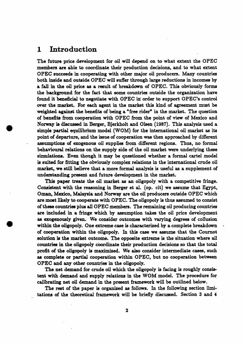
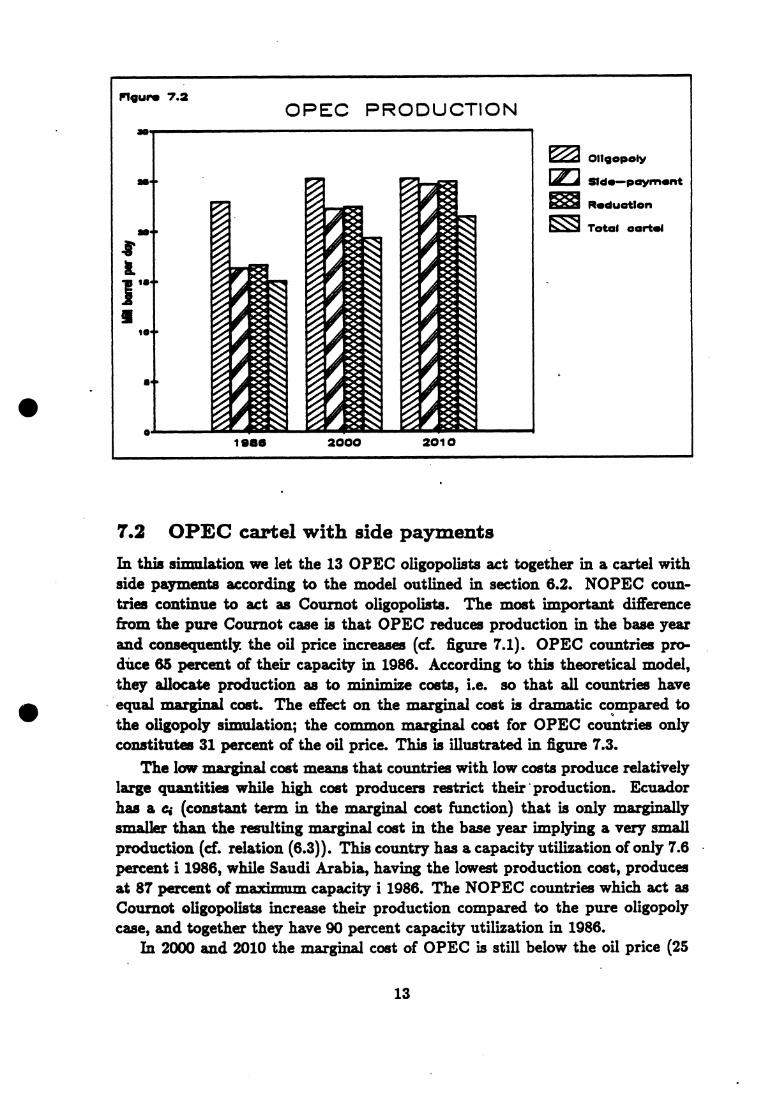
Towards 2000 and 2010 the mourned increase in incomes (GDP) underlyingthe projections imply strong increases in demand. This pushes the capacityutilization rates close to 100 percent in all countries, even high cost countriesproduce more than 97 percent. This puts strong pressure on oil prices, whichrise from 32.70 US$/barrel in 2000 to 86.90 US$/barrel in 2010. Here it should beemphasized that in the presented calculations we have neither taken into accounteffects from competition from other energy sources nor changes in price- andincome responses that probably will occur (especially in developing countries) ifincome and prices rise. The_price paths for the various model simulations areshown in figure 7.1, while the accompanying developments in production fromtoday's OPEC countries are given in figure 7.2.

12

•

7.2 OPEC cartel with side payments

In this simulation we let the 13 OPEC oligopolists act together in a cartel with.side payments according to the model outlined in section 6.2. NOPEC coun-tries continue to act as Cournot oligopolists. The most important differencefrom the pure Cournot case is that OPEC reduces production in the base yearand consequently the oil price increases (cf. figure 7.1). OPEC countries pro-diice 65 percent of their capacity in 1986. According to this theoretical model,they allocate production as to minimize costs, i.e. so that all countries haveequal marginal cost. The effect on the marginal cost is dramatic compared tothe oligopoly simulation; the common marginal cost for OPEC countries onlyconstitutes 31 percent of the oil price. This is illustrated in figure 7.3.

The low marginal cost means that countries with low costs produce relativelylarge quantities while high cost producers restrict their *production. Ecuadorhas a ci (constant term in the marginal cost function) that is only marginallysmaller than the resulting marginal cost in the base year implying a very smallproduction (cf. relation (6.3)). This country has a capacity utilization of only 7.6percent i 1986, while Saudi Arabia, having the lowest production cost, producesat 87 percent of maximum capacity i 1986. The NOPEC countries which act asCournot oligopolists increase their production compared to the pure oligopolycase, and together they have 90 percent capacity utilization in 1986.

In 2000 and 2010 the marginal cost of OPEC is still below the oil price (25

13

•1966 2000 2010

Ths fillod part of oviory bar is marginal costs.zrrErt to that loft, NOPEC to tho right

Figure 7.3OIL PRICES AND MARGINAL COSTS

pricos:

Eal Oligopoly

rzJ Stdo—paymont

EM Total carts.

and 20 percent of price respectively). However, both price and marginal costsincrease, implying that production increases correspondingly. Because of theinverse-L shape of the marginal cost functions for these countries, capacities willbe high even at moderate levels of marginal costs. The capacity utilization in2000 is 87 percent while it is 98 percent in 2010.

All the NOPEC countries. produce close to their capacities in 2000 and 2010.Oman, with low cost oil fields, produce at fall capacity already in the base year.All countries within NOPEC are close to 100 percent of capacity in 2000 andreach 100 percent in 2010. For these countries the marginal costs are close tothe oil price, with the exception of Mexico where marginal costs constitute 90percent of the price.

The oil price is more than 40 percent higher in the base year in this simulationthan in the pure oligopoly case. In 2000 the difference has decreased to 18.5percent and in 2010 the total supply is more or less identical to the oligopolycase which also means that the oil price is about the same.

7.3 OPEC cartel with proportionate reduction of supplies

As described in section 6.3, the other collusive model which we analyze is a hy-pothetical case where all the OPEC oligopolists reduce their production by thesame percent relatively to the market equilibrium in the pure Cournot solution.An important implication of this regime is that marginal costs for OPEC mem-

14

bers no longer are equalized, so that the allocation of total production within thecartel is not carried out in the most efficient way. The z.eduction in productioncompared to the pure oligopoly case is 27 percent in the base year, which is veryclose to the reduced output in the cartel model with side payments. This further-more implies that both the oil price and the total supply from OPEC are almostidentical in the two collusive models. The important difference is the distributionof production within OPEC.

For non-OPEC producers the intuitively reasonable lesson of this outcomeis that what really matters from their point of view is that OPEC act togetherin their struggle for stabilizing and possibly raising the oil price. How suchcoordinate efforts are obtained within OPEC is not that important.

7.4 A cartel model including all 18 oil producers

As mentioned above, during the last years coordinate efforts have been under-taken and some tacit agreements have been obtained even between OPEC andsome non-OPEC oil producers. Even though these contacts obviously are diffi-cult to describe in any formal manner, the existence of such agreements shouldcreate some interest for the present model version.

When the 5 NOPEC countries are included in the cartel, its market powerincreases considerably. This is exploited by the cartel; total output from the 18countries is reduced by 1/3 compared to the oligopoly case in the base year, andby 18 percent from the OPEC-cartel solution. The price is 22.40 US$/barrel inthe base year, an increase of 78 percent compared to the oligopoly case (figure7.1).

In the two OPEC-cartel simulations we saw above that the monopoly powerof the cartel almost vanishes towards 2010, reflected in the observation that theoil price is insignificantly above the value in the pure Cournot case. In the presentsimulation, however, output is reduced in 2010 by 15 percent, while the oil pricein the same year is increased from the Cournot solution by 40 percent (figure7.1).

8 Concluding remarks

The purpose of this paper is to present a framework for analyzing various kinds ofstrategic behaviour and collusive behaviour in the crude oil market. The analysisis preliminary, and in particular the empirical simulations should be regardedmainly as demonstrations of the framework and differences between the variousstrategic models. In these calculations we have e.g. not taken proper accountto the presence of "back-stop" prices and the possibility that income- and price

15

elasticities in LDC countries will change as a results of income growth. Boththese factors will, when implemented, tend to create more realistic levels for theoil price than in the numerical examples presented in this paper. As mentionedabove, we intend to extend the model by relations describing producers decisionswith respect to capacity levels.

As supplements to existing simulation models which are being used for pro-ji.cting the evolution in the crude oil market (among which we may mention theWOM model), we believe that such a framework may show to be very useful as atool for analyzing market developments. This because the models explicitly buildon the fact that strategic behaviour is highly present in the oil market. Used withcare and supplemented with more detailed knowledge to the oil market, we thusregard it as a step towards a better understanding of events in this market.

9 References

Berger, K., O. Bjerkholt and O. Olsen (1987): What are the options fornon-OPEC producing countries. Discussion Paper No. 26, Central Bureauof Statistics, Oslo.

Newbery, D. (1981): Oil prices, cartels and the problem of dynamic incon-sistency. Economic Journal, 91, pp. 617- 646.

Hoel. M. (1981): Resource extraction by a monopolist with influence overthe rate of return on non-resource assets. International Economic Review,22, pp. 147-157.

Hnyilicza, E. and R. Pindyck (1976): Pricing policies for a two-part ex-haustible resource cartel: The case of OPEC. European Economic Review,8, pp. 139454.

d'Aspremont, C., A. Jacquemin, U. Gabszewicz and J. Weym,ark (1.983):On the stability of collusive price leadership. Canadian Journal of Eco-

nomics, 1, pp. 17-25.

Osborne, D.K. (1976): Cartel problems. American Economic Review, 66,pp. 835-844.

16

ISSUED IN THE SERIES DISCUSSION PAPER

No. 1 I. Aslaksen and O. Bjerkholt: Certainty Equivalence Proceduresin the Macroeconomic Planning of an Oil Economy.

No. 3 E. Bjorn: On the Prediction of Population Totals from Samplesurveys Based on Rotating Panels.

No. 4 P. Frenger: A Short Run Dynamic - Equilibrium Model of theNorwegian Prduction Sectors.

No. 5 I. Aslaksen and O. Bjerkholt: Certainty EquivalenceProcedures in Decision-Making under Uncertainty: an EmpiricalApplication.

No. 6 E. Biorn: Depreciation Profiles and the User Cost of Capital.

No. 7 P. Frenger: A Directional Shadow Elasticity of Substitution.

No. 8 S. Longva, L. Lorentsen, and if. Olsen: The Multi-SectoralModel MSG-4, Formal Structure and Empirical Characteristics.

No. 9 J. Fagerberg and G. Sollie: The Method of Constant MarketShares Revisited.

No.10 E. Bjorn: Specification of Consumer Demand Models withStocahstic Elements in the Utility Function and the firstOrder Conditions.

No.11 E. Biorn, E. Holmoy, and O. Olsen: Gross and Net Capital,Productivity and the form of the Survival Function . SomeNorwegian Evidence.

No.12 J. K. Dagsvik: Mlarkov Chains Generated by MaximizingComponents of Multidimensional Extremal Processes.

No.13 E. Morn, M. Jensen, and M. Reymert: KVARTS - A QuarterlyModel of the Norwegian Economy.

No. 14 R. Aaberge: On the Problem of Measuring Inequality.

No.I5 A-M. Jensen and T. Schweder: The Engine of FertilityInfluenced by Interbirth Employment.

No.16 E. Bjorn: Energy Price Changes, and Induced Scrapping andRevaluation of Capital - A Putty-Clay Approach.

No.17 E. Bi sm and P. Frenger: Expectations, Substitution, andScrapping in a Putty-Clay Model.

No.18 R. Bergan, R. Cappelen, S. Longva, and N. M. Stolen: MODAG A-A Medium Term Annual Macroeconomic Model of the NorwegianEconomy.

No.19 E. Morn and H. Olsen: A Generalized Single Equation ErrorCorrection Model and its Application to Quarterly Data.

17

No.20 K. H. Alfsen, O. A. Hanson, and S. Glomsrod: Direct andIndirect Effects of reducing SO Emissions: ExperimentalCalculations of the MSG-4E Model. 2

No.21 J. K. Dagsvik: Econometric Analysis of Labor Supply in a LifeCycle Context with Uncertainty.

No.22 K. A. Brekke, E. Gjelsvik, B. H. Vatne: A Dynamic Supply SideGame Applied to the European Gas Market.

No.23 S. Bartlett, J. K. Dagsvik, O. Olsen and S. Strom: Fuel Choiceand the Demand for Natural Gas in Western European Households.

No.24 J. K. Dagsvik and R. Aaberge: Stochastic Properties andFunctional Forms in Life Cycle Models for Transitions into andout of Employment.

No.25 T. J. Klette: Taxing or Subsidising an Exporting Industry.

No.26 K. J. Berger, O. Bjerkholt and O. Olsen: What are the Optionsfor non-OPEC Producing Countries.

No.27 A. Aaheim: Depletion of Large Gas Fields with Thin Oil Layersand Uncertain Stocks.

No.28 J. K. Dagsvik: A Modification of Heckman's Two StageEstimation Procedure that is Applicable when the Budget Set isConvex.

No.29 K. Berger, K. Cappelen and I. Svendsen: Investment Booms in anOil Economy - The Norwegian Case.

No.30 A. Rygh Swensen: Estimating Change in a Proportion byCombining Measurements fram a True and a Fallible Classifier.

No.31 J.K. Dagsvik: The Continuous Generalized Extreme Value Modelwith Special Reference to Static Models of Labor Supply.

No.32 K. Berger, M. Hoel, S. Holden and O. Olsen: The Oil Market asan Oligopoly.

18