The Optimal Monetary Policy Rule for the European Central Bank

Paolo Gelain†

Department of Economics – University of Pisa

January 2007 Abstract. In this paper we derive the optimal monetary policy rule for the European Central Bank (ECB), solving a minimization problem in which the Central Bank minimizes a (quadratic) loss function (whose arguments are inflation, output gap and the interest rate lag), subject to the constraint given by a model representing the economy which the Bank refers to. We used the algorithm to solve stochastic discounted optimal linear regulator problems. The interest rate is the policy instrument and the policy rule we derive shows the following main features: 1) the coefficient suggested as response of the interest rate to the current inflation is less than one, hence smaller then what indicated by the well known Taylor rule; 2) it is optimal for the ECB to allow for a high degree of policy gradualism or interest rate smoothing. Moreover, the use of our derived optimal rule guarantees much less variability of inflation and output gap responses to an interest rate shock. † e-mail: paologelain@yahoo.it p.gelain@ec.unipi.it

2

CONTENTS

INTRODUCTION……………………………………………………………………………..4

1. THE ECB: OBJECTIVES, RULES AND MONETARY POLICY………………………...6

2. THE MODEL OF THE EUROPEAN ECONOMY

2.1. Motivations……………………………………………………………………......8

2.2. Theoretical issues……………………………………………………………….....9

2.3. Empirical results………………………………………………………………....12

2.4. Comparison with other models…………………………………………………..13

2.5. Stability tests……………………………………………………………………..16

3. COMPUTATION OF THE OPTIMAL RULE

3.1. The model………………………………………………………………………..19

3.2. State-space representation………………………………………………………..22

3.3. Solving the model………………………………………………………………..24

4. ANALYSIS OF THE OPTIMAL RULE

4.1. Efficiency frontier………………………………………………………………..30

4.2. Dynamic response………………………………………………………………..32

CONCLUSIONS……………………………………………………………………………..35

3

APPENDICES

Appendix A. Dynamic Programming………………………………………………37

Appendix B. Derivation of the loss values…………………………………………39

REFERENCES……………………………………………………………………………..40

FIGURES AND TABLES………………………………………………………………….44

4

INTRODUCTION

In this paper we want to derive the optimal monetary policy rule for the European Central

Bank (ECB). Loosely speaking we want to derive a rule which can be used by the ECB to

optimally set the interest rate, which we are going to assume the instrument used to

implement monetary policy, in response to the variations of the main variables we consider

relevant for the ECB, i.e. inflation and output gap (as a measure of the economic activity), in

terms of minimization of a loss function which characterizes the preferences of the central

bank about the variability of those variables. The economic environment will be the constraint

of the ECB.

The main reason why we think that it is worth developing this paper is that we found just

one paper which derives an optimal rule for the ECB (Peersman and Smets (1998)) like us.

However, the sample period that has been used goes from 1975 to 1997, like in all the others

works regarding the monetary policy rules for the euro area, in which however rules are

estimated rather that optimally derived. This approach may suffer of the drawback that the

answer to the question “does it make sense to do monetary policy analysis with respect to a

Central Bank taking into account a period in which that Central Bank does not exist?” is

“probably it does not”. In fact, we will show that our results imply quite different policy

suggestions for the ECB with respect to those of Peersman and Smets (1998). In particular,

those differences crucially depends on the changed features of the euro area in the recenr

years, especially in terms of persistence of inflation. Actually our sample is from 1995 to

2003, and apparently it is interested by the same kind of critique, but in what follows we will

extensively explain why we think that it is not true.

Moreover, there is another good reason to develop our work. There are some papers (see

for instance Breuss (2002), Galí et al. (2004), and Ullrich (2003)) which estimate rules trying

to overcome the problem of the sample period, focusing on years when ECB “is at work”, i.e.

after 1999. However, they may suffer of the fact that data are not enough to estimate properly

the model of the economy. Besides, we did not find anyone deriving the optimal rule.

Hence, taking into account these two first motivations, we see our sample as a good

compromise between the need to have enough observations and a reasonable historical period

considered.

Further, my work is different from the others in two respects. In fact, since before 1998

euro area did not exist, there are no proper data for it. The most part of datasets are

constructed aggregating the variables of interest of the single European countries, often

5

considering 3 or 5 representative countries. These are forms of approximation which may lead

to lack of reliability. Hence we have decided to adopt the dataset created by Fagan et al.

(2001) who propose the Area Wide Model in which 11 European countries are taken into

account and aggregated following the “Index method” (see the paper for further details). What

it is important to note is that our geographic euro aggregate better reflects the euro area

composition.

In the end, since data before 1995 are not reliable, whatever aggregation one uses, my data

set has the advantage of being more reliable than the ones used in other works.

The approach we are going to use to derive the optimal rule is not new in the literature. It

is a simple application of the algorithm to solve stochastic discounted optimal linear regulator

problems (see Ljungqvist and Sargent (2004)). Basically the problem consists in a

minimization of a (quadratic) loss function, which is the objective function of the monetary

authority (ECB in our case) subject to the constraint represented by the economy which the

authority refers to.

Solving that problem, it is possible to derive the optimal policy rule, i.e. a rule which can

be used by the ECB to optimally set the interest rate given the state of the economy and the

relationships between the economic variables representing it.

We develop five sections. In the first one we briefly describe the role and the objectives of

the ECB. The second section is devoted to present and estimate the model of the European

economy, which will be the constraint of the maximization problem. In the third section, after

giving the motivation to consider the loss function we considered, we set it and the state space

representation in order to derive the optimal rule; then we derive it. The fourth section

concerns the analysis of the optimal rule, its dynamic properties, its macroeconomic

performance and its comparison with the Taylor rule. In the fifth, we briefly compare the

optimal behaviour of ECB with what it has really done. Some concluding remarks close this

work.

6

1. THE ECB: OBJECTIVES, RULES AND MONETARY POLICY

Article 105 of the Maastricht Treaty of 1992 clearly establishes which is the aim of the

European Central Bank. It states that “the primary objective of the ESCB1 is to maintain price

stability. Without prejudice to this objective, it shall support the general economic policies in

the Community with a view to contributing to the achievement of the objectives of the

Community [which include a high level of employment and sustainable and non-inflationary

growth]. Furthermore, the ESCB shall act in line with the principle of an open market

economy with free competition”.

Although clear enough, the article is quite vague for what concerns the definition of price

stability. In fact, in October 1998 the Governing Council of the ECB defined price stability as

“a year-on-year increase in the Harmonised Index of Consumer Prices (HICP) for the euro

area of below 2%” and added that price stability “was to be maintained over the medium

term” . The Governing Council confirmed this definition in May 2003 following a thorough

evaluation of the ECB’s monetary policy strategy. On that occasion, the Governing Council

clarified that “in the pursuit of price stability, it aims to maintain inflation rates below but

close to 2% over the medium term”.

What it is important to underline at this point for the purposes of our analysis is that the

ECB has been charged with the responsibility of the maintenance of price stability, but at the

same time it has to care about other objectives, like economic growth.

Having defined a target for inflation, may imply that ECB works in a regime of inflation

targeting. As a matter of fact definition of inflation targeting is not unique since many give

different and sometimes conflicting definitions, but there are some criteria which one has to

look for to define inflation targeting. In particular, quoting Mishkin (2001) “[i]nflation

targeting is a recent monetary policy strategy that encompasses five main elements: 1) the

public announcement of medium-term numerical targets for inflation; 2) an institutional

commitment to price stability as the primary goal of monetary policy, to which other goals

are subordinated; 3) an information inclusive strategy in which many variables [among

which inflation forecast may have an important role] 4) increased transparency of the

monetary policy strategy through communication with the public and the markets about the

plans, objectives, and decisions of the monetary authorities; and 5) increased accountability

of the central bank for attaining its inflation objectives”.

1 European System of Central Banks.

7

In this work we don’t want to investigate whether or not the ECB is an inflation targeter.

In particular because “while there are many similarities between the ECB’s strategy and

strategies of other central banks using inflation targeting, the ECB decided not to pursue a

direct inflation targeting strategy in the sense discussed above for a number of reasons”2,

basically related to the problems associated with inflation forecast.

For what concerns the policy rules, we want to highlight, although not properly correct,

that to an inflation target regime is associated a policy rule which the central bank follows to

achieve its targets. As it is known, the policy process is too complex to be represented by a

simple monetary rule, but apart the general consensus of central bankers on the fact that

policy rules can be a good guidance for monetary policy, also the EBC does not seem to

totally reject the usefulness of monetary policy rules. In fact, in its Monthly Bulletin of

October 2001 (ECB 2001, p. 38), the ECB states: “The emphasis … on rule-guided monetary

policy … is generally welcome [because] it provides a salutary antidote to the perennial risks

of a discretionary, ad hoc approach to monetary policy”. This statement by itself provides

enough motivation for the search of the monetary policy rule of the ECB.

2 European Central Bank (2004).

8

2. THE MODEL OF THE EUROPEAN ECONOMY

2.1. Motivations

There is a number of motivations to estimate a simple model like the one we propose later

on. Most of them are underlined in Rudebucsh and Svensson (1998), hence in reporting them

we will draw heavily from that paper. Moreover, we will add a couple of reasons to

strengthen our argument.

First of all, our model is composed of just two equations, an IS curve and a Phillips curve

which represent the demand and the supply side of the economy respectively. This allows for

more transparent results, but it may create problems for what concerns the richness of the

dynamic incorporated in it. However we will see that from a comparison with richer models

(i.e. VAR) our model performs in a satisfactory way. This kind of comparison may also be

good in terms of fit to data, since VAR is a tool that allows data to speak as much as possible.

Second, simple models capture the spirit of many policy oriented macroeconometric

models. If this is true for many central bankers, as it can be seen in the 11 models described in

the central bank comparison project for the Bank for International Settlements3, it is also quite

true for the ECB which has not a formal model4 used for the euro area analysis, although

some economists of the Institute provided some of them, and as we will see later on half of

them are based on simple structural equations.

In the end we can add the following reasons. First we argue that simple models are in line

with the recent macroeconomic theory regarding the New Keynesian general equilibrium

models5. In fact, despite their derivation, which is something mathematically very articulated

and refined, they end up with two equations, i.e. the forward looking version of both the IS

and Phillips Curve.

Second, a very simple argument may be that the main aim of this work is not to estimate a

model of the euro area, but rather to derive the optimal policy rule for the ECB.

3 See Bank for International Settlements (1995). 4 This means that it has not a model that everyone knows it is the ECB model, like for instance the FRB/US model (substituted by the MPS model in 1996) which is the Federal Reserve Board’s main quarterly macroeconometric model. 5 The two masterpieces on the subject are Clarida, Gali and Gerlter (1999) and Goodfriend and King (1997).

9

2.2. Theoretical issues

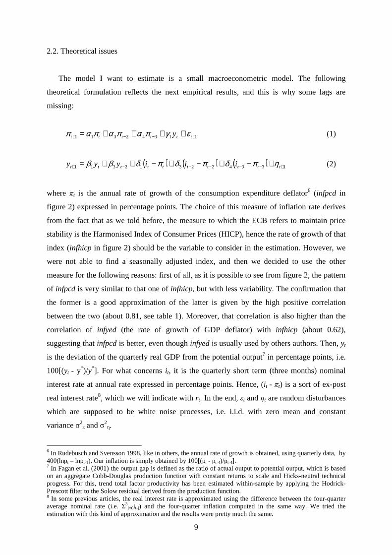
The model I want to estimate is a small macroeconometric model. The following

theoretical formulation reflects the next empirical results, and this is why some lags are

missing:

11342311 +−−+ ++++= tttttt y εγπαπαπαπ (1)

( ) ( ) ( ) 133422312311 +−−−−−+ +−+−+−++= tttttttttt iiiyyy ηπδπδπδββ (2)

where πt is the annual rate of growth of the consumption expenditure deflator6 (infpcd in

figure 2) expressed in percentage points. The choice of this measure of inflation rate derives

from the fact that as we told before, the measure to which the ECB refers to maintain price

stability is the Harmonised Index of Consumer Prices (HICP), hence the rate of growth of that

index (infhicp in figure 2) should be the variable to consider in the estimation. However, we

were not able to find a seasonally adjusted index, and then we decided to use the other

measure for the following reasons: first of all, as it is possible to see from figure 2, the pattern

of infpcd is very similar to that one of infhicp, but with less variability. The confirmation that

the former is a good approximation of the latter is given by the high positive correlation

between the two (about 0.81, see table 1). Moreover, that correlation is also higher than the

correlation of infyed (the rate of growth of GDP deflator) with infhicp (about 0.62),

suggesting that infpcd is better, even though infyed is usually used by others authors. Then, yt

is the deviation of the quarterly real GDP from the potential output7 in percentage points, i.e.

100[(yt - y*)/y*]. For what concerns i t, it is the quarterly short term (three months) nominal

interest rate at annual rate expressed in percentage points. Hence, (i t - πt) is a sort of ex-post

real interest rate8, which we will indicate with r t. In the end, εt and ηt are random disturbances

which are supposed to be white noise processes, i.e. i.i.d. with zero mean and constant

variance σ2ε and σ2

η.

6 In Rudebusch and Svensson 1998, like in others, the annual rate of growth is obtained, using quarterly data, by 400(lnpt – lnpt-1). Our inflation is simply obtained by 100[(pt - pt-4)/pt-4]. 7 In Fagan et al. (2001) the output gap is defined as the ratio of actual output to potential output, which is based on an aggregate Cobb-Douglas production function with constant returns to scale and Hicks-neutral technical progress. For this, trend total factor productivity has been estimated within-sample by applying the Hodrick-Prescott filter to the Solow residual derived from the production function. 8 In some previous articles, the real interest rate is approximated using the difference between the four-quarter average nominal rate (i.e. Σ3

j=0i t-j) and the four-quarter inflation computed in the same way. We tried the estimation with this kind of approximation and the results were pretty much the same.

10

All variables are demeaned before estimation, hence no constants appear in the equations.

The first equation is a Phillips Curve. It can be viewed as a supply curve since it relates

the inflation rate with its own lags and the lags of the output gap. What it is important to note

is that the expectations are assumed to be adaptive. This formulation is compatible with the

idea of a constant equilibrium value of the real output, which we assume here on computing

the potential output, if the Phillips Curve is vertical in the long run. This is assured if the sum

of the parameters of the lagged values of the inflation in equation 1 is equal to one. Later on

we will see that this hypothesis is not rejected by our data.

Moreover, there are some arguments that it is useful to report to justify the use of adaptive

expectations, rather than other forms (e.g. rational ones). In the first instance, some central

bankers (like for instance Alan Blinder, Federal Reserve Governor) appear more comfortable

with backward looking version, as demonstrated by many models used by them. Second,

Taylor (1993) and Bofim and Rudebusch (1997) sustain that in a period of transition to a new

monetary policy, the adaptive expectations may be more realistic than the rational ones, since

people are try to learn the new central bank behaviour. The same kind of argument can be

extended to the ECB, since it is a relative young institution and the agents may be still trying

to learn about its policy. As a matter of fact, the objective of the ECB is clear enough to allow

agents to form expectations about its policy. However, sometimes it is not clear if the ECB

monetary policy is either discretionary or linked to some form of commitment9. In the end, for

the US economy it has been found that backward looking models require relatively more

aggressive policies with at most moderate inertia; rules that are optimised for such models

tend to perform reasonably well in forward looking models, while the reverse is not necessary

true10; Adalid et al. (2005) found same results for the euro area.

What we also report is the fact that although a large literature is in favour of the New

Keynesian Phillips curve11, which is the version which explicitly takes into account for

rational expectations, there are many papers in which autoregressive Phillips curves are tested

against forward looking versions and they cannot reject the hypothesis that the former holds12.

Equation (2) is a IS Curve, which represents the demand side of the economy. It relates

the output gap with its own lags and with the lags of the real interest rate. The latter

synthesizes the transmission mechanism of the monetary policy to the real economic activity

9 See for instance Monacelli (2005). 10 See Bryant et al. (1993), Taylor (1999), Levin et al. (1999). 11 See for instance Gali and Gerltler (1999) and Gali (2001) for what concerns the estimation of the New Keynesian Phillips Curve. 12 Among others, Fanelli (2005) and the references therein. They are similar but the latter is an extension of the former since it uses the same database but with more years, part of which is exactly the years of our sample.

11

and to the price level. As a matter of fact the transmission mechanism is more complicated in

the euro area, as can bee seen in figure 3, involving also possible effects of changes in money

markets rates on financial asset prices, such as share prices or exchange rate which in turn act

on the saving and investment decisions of households and firms. Moreover wealth and income

effects can arise from changes in asset prices. Expectations on future inflation rate are also an

important channel. However the same figure shows that there is a clear and direct link

between the official interest rate and the markets rates. This allows us to consider the interest

rate as the instrument used by the ECB to conduct monetary policy. To further confirm that

short term interest rate is a good proxy for the ECB policy instruments, we can look at figure

4 to verify that the ECB can really control the market interest rate. As a matter of fact, the

evolution of the latter is closely related to the main refinancing operation rate, which is the

official rate used for the implementation of the monetary policy, i.e. it is the rate which the

ECB control directly.

Our estimation refers to the period 1995Q1 to 2003Q4. The choice of the period is

motivated by different reasons. On the first place, data from Fagan et al. were available only

up to 2003. Moreover, the reliability of the data is assured just from 1995.

On the other hand, all the works done on the derivation of an optimal rule for the ECB up

to now are based on a sample period starting in the 1970s and ending in the 1990s. Basing on

such a long period, estimates can be more accurate, but one may wonder whether it makes

sense to do monetary policy analysis for a period during which the Central Bank did not exist.

My sample period is interested by the same kind of critique since ECB was born in 1999.

However, some characteristics of the economic variables during the period 1995 1998 suggest

that European countries were already following a sort of unique monetary policy which

features were very close to the current ones, at least as long as the objectives are concerned.

The Maastricht Treaty of 1992 accelerated the process of monetary convergence imposing

criteria on the level of interest an inflation rate. This is confirmed by figure 5 where are

depicted the monetary market interest rates of Germany, France and Italy. The high positive

correlation (see table 2) between those rates can also suggest that monetary policies were

similar in those countries. In the end, the high variances of the output gaps and the low

variances of the inflation rates (see table 3) may imply equal monetary policy objectives, i.e.

that policies were more inflation stabilization oriented.

In the end, no important structural changes has occurred in the euro area during our

sample period, except for the creation of the euro area, but this doesn’t seem to have created

12

change in the European economy13, since the process of monetary integration had starting to

taking place several years before.

2.3. Empirical results

To obtain our results we mainly use a general to simple approach based on the information

criteria comparison. Moreover, we put attention on the individual statistical and economical

significance of the coefficients, on the goodness of fit (R2 and adjusted R2), on the correlation

between actual and fitted values and on the appropriateness of the tests statistics regarding

autocorrelation (LM test) and normality of OLS residuals and presence of heteroskedsticty. A

Reset test has also been implemented to test eventual misspecifications (even though it can

have low power).

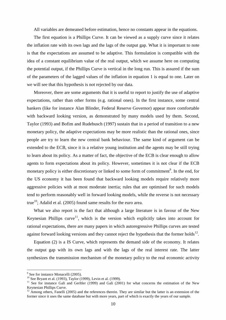
Our estimation results are (standard errors in parenthesis):

1321 091.0391.0595.0034.1 +−−+ +++−= tttttt y εππππ (3)

(0.1462) (0.2239) (0.1969) (0.05868)

# obs.=36, R2=0.791288, Adjusted R2=0.768926, σε=0.185, AR (1-3) test: F(3,25)=0.44800 [0.7209], Normality test: χ2(2)=1.0371 [0.5954], heteroskedasticity test: F(8,19)=1.1938 [0.3533],

RESET test: F(1,27)=0.79620 [0.3801], correlation between actual and fitted values: 0.88957.

( ) ( ) ( ) 1332221 315.0503.0274.038.0234.1 +−−−−−+ +−−−+−−−= tttttttttt iiiyyy ηπππ (4)

(0.1109) (0.1085) (0.1129) (0.2120) (0.1596)

# obs.=36, R2=0.909528, Adjusted R2=0.896125, ση=0.2674, AR (1-3) test: F(3,24)=1.0820 [0.3755], Normality test: χ2(2)=1.9964 [0.3685], heteroskedasticity test: F(10,16)=0.48865 [0.8737],

RESET test: F(1,26)=0.81920 [0.3737], correlation between actual and fitted values: 0.95358.

Rejection of null hypothesis is marked with * and ** for 5 and 1 per cent significance

level respectively.

Estimation has been done separately using OLS, but similar results could be obtained

estimating a system of equations, since the cross-correlations of the residuals are essentially

zero.

Both the estimations display a good fit to data since R2s are very high and close to 1. Also

the correlation with fitted data is good. All tests suggest absence of autocorrelation, of non

13 See for instance Clausen and Hayo (2002).

13

normality in the residuals and of heteroskedasticity. This allows us to rely upon inference

drawn from the standard errors. In particular, all coefficients are highly statistically

significant, except for the first lag of output gap in equation (3) which however is significant

at 10 per cent significance level. For a comparison of our results with those of others authors

in terms of significance of the coefficients see table 4.

As for the restriction on the lagged values of inflation in equation (3), the χ2 statistics is

χ2(1) = 3.17189 [0.0749], hence we cannot reject the null hypothesis of a vertical Phillips

Curve.

Two main features emerge from these results. First, inflation displays a quite high

persistence. In fact, the sum of all the coefficients of the lags is equal to 0.83. This is in line

with the recent findings of the Inflation Persistence Network, whose analysis focus on

measuring and comparing patterns of price setting and inflation persistence in the euro area14,

and in this respect inflation is more persistent that what found by Peersman and Smets (1998).

In fact, they obtain a sum of the autoregressive coefficients equal to 0.74 (see table 4).

Nevertheless, we have to underline at this stage that here the meaning of persistence has to be

interpreted as the time needed to a variable to come back to its equilibrium value after a

shock, and in this other respect, inflation is less persistent, because in my case it comes back

much earlier than in Peersamn and Smets (see fig.6b and the next paragraph for further

details).

On the other hand, there is a low role of the output gap in explaining inflation. In fact the

coefficient is low and not highly significant.

These two characteristics will be fundamental in order to obtain my results in terms of

optimal rule.

2.4. Comparison with other models

The estimation of simple models characterized by the presence of only few variables may

have some drawbacks. In particular it may be subject of the following critiques:

a) it can be a poor representation of the economic system which it refers to, failing to

capture its salient characteristics;

b) it may lack to account for the right dynamic relationship between variables.

14 See Angeloni et al. (2005).

14

In order to avoid the first drawback it may be useful to compare our model with other

estimated structural models regarding the same economic environment, while the second

objection may be faced by considering an unrestricted VAR.

As already said, the ECB has not a formal model used for economic analysis. As

summarized in Adalid et al. (2005), structural models for the euro area are essentially four:

1) the Coenen-Wieland model (see Coenen and Wieland, 2000) is a small-scale model

of aggregate supply and aggregate demand which is designed to capture the broad

characteristics of inflation and output dynamics in the euro area.

2) The Smets-Wouters model (see Smets andWouters, 2003) is an extended version of

the standard New-Keynesian DSGE closed-economy model with sticky prices and wages. The

model is estimated by Bayesian techniques using seven euro area macroeconomic time series:

real GDP, consumption, investment, employment, real wages, inflation and the nominal short-

term interest rate.

3) The Area-Wide Model (see Fagan et al., 2001) is a medium-size structural

macroeconomic model that treats the euro area as a single economy. It has a long-run neo-

classical equilibrium with a vertical Phillips curve but with some short-run frictions in price

and wage setting and factor demands.

4) The Dis-aggregate Model of the euro area used in Angelini et al. (2002) and

Monteforte and Siviero (2002) is a multi-country version of the simple backward-looking two

equations model in Rudebusch and Svensson (1999). It consists of an aggregate supply

equation and an aggregate demand equation for each of the three largest economies in the

euro area; i.e., Germany, France and Italy.

There are two types of comparisons we can implement. With backward-looking models

(i.e. the first one and the fourth one) we can compare both the coefficients and the impulse

response functions (especially for what concerns the response to monetary policy shocks),

while with forward-looking model just in terms of impulse response functions.

The coefficients of the comparable model are reported in table 4. Other model estimates of

the euro area are reported together with one of the United States. The sample period of those

estimations is larger and it precedes ours. This last fact may justify the differences in the IS

curve estimation, even though Coenen and Weiland (2000) obtain similar results and the

model for United States as well. The dynamics of the interest rate is also quite different

(richer) from all others.

As for the Phillips Curve, differences are clear. Our equation shows that inflation displays

much less inertia then the previous ones, i.e. shocks that hit inflation are less persistent.

15

Again, this is in line with the recent findings of the Inflation Persistence Network. They found

that “…an unexpected monetary policy change has a short-lived effect on euro area real

output, which peaks around 4-6 quarters after the shock and then dissipates relatively quickly.

By contrast, the aggregate price level in the economy is affected more gradually but

permanently… An interpretation of this evidence is that the inflation process in the euro area

is subject to higher degree of rigidity, possibly due to a less competitive environment, more

extensive price regulation or other formal or informal constraints on price setters”. In fact

looking at the impulse response functions15 in figure 6b, we can easily see that all the

responses have the expected sign (in particular those of output and inflation to interest rate).

The response of output gap reaches a pick after three quarters and it comes back to the

equilibrium after eleven quarters; whereas inflation reverts its negative path after 6-7 quarters,

to reach the equilibrium after only about 20 quarters. Similar responses are obtained by richer

structural models, e.g. either Smets and Wouters (2003) or Fagan et al. (2001), at least from

the point of view of the signs of the responses.

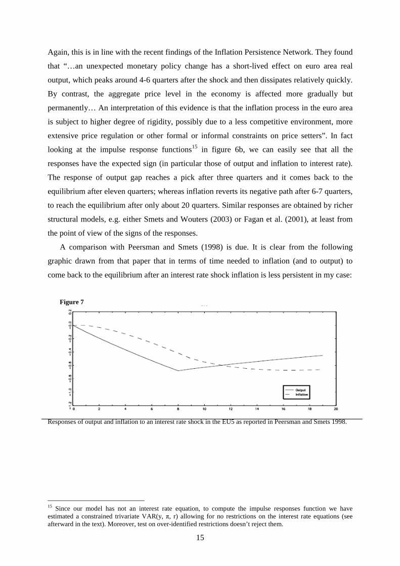
A comparison with Peersman and Smets (1998) is due. It is clear from the following

graphic drawn from that paper that in terms of time needed to inflation (and to output) to

come back to the equilibrium after an interest rate shock inflation is less persistent in my case:

Figure 7

Responses of output and inflation to an interest rate shock in the EU5 as reported in Peersman and Smets 1998.

15 Since our model has not an interest rate equation, to compute the impulse responses function we have estimated a constrained trivariate VAR(y, π, r) allowing for no restrictions on the interest rate equations (see afterward in the text). Moreover, test on over-identified restrictions doesn’t reject them.

16

Impulse response functions in figure 6b can be compared with the impulses from a VAR16

with output gap, inflation and real interest rate17 as endogenous variables with four lags18. In

fact our structural model can be viewed as a two restricted equations from the trivariate VAR.

Figures 6a and 6b shows that the estimation of a parsimonious model doesn’t lead to loss in

the dynamic features of the system, given that most of the responses are pretty much the

same. Moreover, the response of the inflation to interest rate is even more satisfactory, since it

has the right sign, contrary to the one of the VAR.

As a final comparison between our structural model and the VAR, table 5 below reports

the information criteria of our equations and those of the single equations of the VAR. The

main criteria on which we base the comparison are the Schawrz (SC) and Akaike Information

Criteria (AIC). As a matter of completeness we report also the Hannan-Quinn (HQ) and Final

Prediction Error (FPE) criteria. The formers are functions of the residual sum of squares and

they are differentiated by their degrees of freedom penalty for the number of parameters

estimated. The SC more heavily penalizes extra parameters. As shown in table 5, the

structural model’s inflation equation is favoured over the VAR’s inflation equation by both

the SC and AIC (even by the other criteria). The SC favours the structural output equation,

while the AIC favours the VAR. Overall, the information criteria do not appear to view our

structural model restrictions unfavourably.

Table 5. INFORMATION CRITERIA

AIC SC HQ FPE

Structural inflation

equation -12.3805 -12.1973 -12.3198 4.20508e-006

VAR’s inflation

equation -12.0170 -11.3757 -11.8044 6.43514e-006

Structural output

equation -11.6954 -11.4663 -11.6195 8.35389e-006

VAR’s output

equation -11.8709 -11.2296 -11.6583 7.44756e-006

Both the highest absolute value for negative numbers and the smallest value for positive numbers suggest that the associated equation is preferable.

16 The impulse response functions are obtained considering a Cholesky decomposition, i.e. according with the order of the variables chosen in the estimation this implies that shocks to interest rate have not a contemporaneous effect on output and inflation, but just lagged. The same kind of decomposition is used in Peersman and Smets (2001). 17 Usually the impulse response function to analyse an interest rate shock when this is used as a monetary policy instrument is computed from a VAR in which the nominal interest rate appears as endogenous variable. Therefore, using here the real one doesn’t give us different results. 18 The number of lags has been chosen in accordance with the maximum lag of the structural equations, which is exactly four.

17

2.5. Stability tests

The analysis of the stability of the parameter is essential to avoid being “victims” of the so

called Lucas Critique (1976). In fact in his article, Lucas stated that “given that the structure

of an econometric model consist of optimal decision rules of economic agents, and that

optimal decision rule vary systematically with change in the structure of series relevant of the

decision maker, it follows that any change in policy will systematically alter the structure of

econometric models”. In other words, quantitative evaluations of alternative economic

policies based on reduced form (like the one we are proposing) do not provide any useful

piece of information and may even be misleading.

In particular, the Lucas Critique is particularly strong when considering backward looking

models. In fact, one of the remedy is to build models with rational expectations (or forward

looking models), since those models seem safe from the critique, although Estrella and Fuhrer

(1999) provide empirical evidence for greater stability of estimations based on backward-

looking rather than on forward looking models.

Some test the Lucas critique using the exogeneity and the super-exogeneity tests proposed

by Engle, Hendy and Richard (1983), but recent works (see e.g. Lindé (1999) among others)

underline the lack of power of super-exogeneity tests.

In the end, to justify the tests we are going to propose, we quote Lubik and Surico (2006)

who argue that “tests for parameter stability in backward-looking specifications or reduced

forms of macroeconomic relationships typically fail to reject the null of structural stability in

the presence of well-documented policy shifts. This evidence would support the conclusion

that policy changes are … ‘modest’ enough not to alter the behaviour of private agents in a

manner that is detectable by the econometrician. A further implication is that backward

looking monetary models of the type advocated by Rudebusch and Svensson (1998), which

perform well empirically, are safe to use in policy experiments”.

Since it seems that there is no consensus on whether Lucas critique is important or not and

on which tests to use to test it, we proceed with some common tests to check the stability of

our model. Tests we will implement are particularly useful because they are based on the idea

that a regime change might take place slowly, and at un unknown point in time, or that the

regime underlying the observed data might simply not be stable at all, contrary to the more

common tests on structural breaks such as the Chow test.

The main test which we rely upon is the test proposed by Hansen (1992). This test is

based on the algebraic properties of the cumulative sum of the least square estimation. For

18

particularly high19 values of the test the null hypothesis of model stability is rejected. Table 6

below reports the Hansen statistics and they indicate stability for both the equations.

Table 6. HANSEN TESTS

Variance joint Individual parameters tests

Inflation’s equation 0.21700 0.54632

α1 0.056182

α3 0.039964

α4 0.081917

γ1 0.061552

Output gap’s equation 0.025497 0.58377

β1 0.048403

β3 0.043172

δ1 0.18656

δ3 0.10825

δ4 0.13735

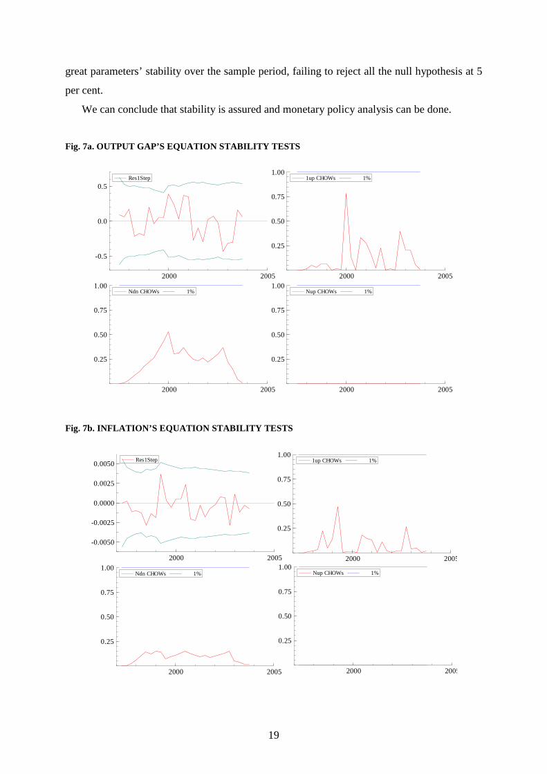
To further confirm this first results, we proceed in computing some recursive tests. In

particular, figures 7a and 7b show the 1-step residual bordered by 0±2s^t over M,...,T, where

s^t is the standard error and M and T are two points inside the sample. In our case they are

1997Q3 and 2003Q4 respectively. Points outside the 2 standard-error region are either

outliers or are associated with coefficient changes, and as it is possible to see there are not

outside points for both equations. Then, we propose three variants of the Chow test: 1-Step

Chow tests, Break-point Chow tests and Forecast Chow tests. All of them are computed for

all t = M,…,T. The last two are distinguished from the fact that they are computed from the

end to 1 and from the beginning to the end. They are distributed as F(1,t-k-1), F(T-t+1,t-k-1),

F(t-M+1,M-k-1), where k is the number of regressors. As it is in general for the recursive

analysis, results are better reported using graphics; in fact figures 7a and 7b report also those

associated with the tests just described. For what concerns the output gap equation, all tests

indicate that the null hypothesis of stability during the period cannot be rejected20 at 1 per cent

significance level. Test at 5 per cent show similar results, except for just a rejection regarding

the 1-step Chow tests at t = 2000Q1, but this cannot compromise our conclusion of substantial

stability of the parameters. Turning on the inflation equation, all the recursive tests assure 19 Hansen provides asymptotic critical values for the test of model consistency. In PcGive the rejection of the null hypothesis is marked with an asterisk and here as well. 20 Tests are scaled by 1-off critical values from the F-distribution at any selected probability level as an adjustment for changing degrees of freedom, so that the significant critical values become a straight line at unity. In other words, if the test line crosses that strait line it means rejection of the null at the significance level indicated in the up-left corner label.

19

great parameters’ stability over the sample period, failing to reject all the null hypothesis at 5

per cent.

We can conclude that stability is assured and monetary policy analysis can be done.

Fig. 7a. OUTPUT GAP’S EQUATION STABILITY TESTS

2000 2005

-0.5

0.0

0.5Res1Step

2000 2005

0.25

0.50

0.75

1.001up CHOWs 1%

2000 2005

0.25

0.50

0.75

1.00Ndn CHOWs 1%

2000 2005

0.25

0.50

0.75

1.00Nup CHOWs 1%

Fig. 7b. INFLATION’S EQUATION STABILITY TESTS

2000 2005

-0.0050

-0.0025

0.0000

0.0025

0.0050Res1Step

2000 2005

0.25

0.50

0.75

1.001up CHOWs 1%

2000 2005

0.25

0.50

0.75

1.00Ndn CHOWs 1%

2000 2005

0.25

0.50

0.75

1.00Nup CHOWs 1%

20

3. COMPUTATION OF THE OPTIMAL RULE

3.1. The model

The computation of an optimal policy rule passes through the maximization (or

minimization) of an objective (loss) function by the Central Bank in which some variables are

taken as objectives subject to a constraint. The choice of the objectives which a Central Bank

has to care about in its loss function is not straightforward. The most common variables

considered in the literature are inflation rate, some measures of the economic activity (e.g.

output gap), and first differences of interest rate to include the interest rate smoothing21

preferences. In fact this is what we propose below.

However, some other variables may be justified case by case. In particular, if the central

bank has different targets beyond those of inflation and output stabilization, the deviations

from those other targets may enter in the loss function. For instance, exchange rate is usually

a good candidate for relatively open economies. Nevertheless, as suggested by Taylor (?), for

the United States including the exchange rate in the loss function (or in the policy rule, which

is the same) worse the macroeconomic performances of the policy rule, measured in terms of

fluctuations of inflation and output gap around their targets. Moreover Ball (1999), Svensson

(2000) and Taylor (1999) find that including the exchange rate was quite useless in terms of

improvement of economic performances. This is because assuming rational expectations the

effects of a variation of the exchange rate today is reflected in a change in the expectations on

future output and inflation, which in turn leads to a change in the expectation of the future

interest rate, which lastly implies a change in the actual interest rate. Our model has not

rational expectations, but there is another explanation which can be used: the short run

fluctuations of exchange rate cannot have a large effect the inflation so that no Central Bank

reaction is necessary.

Another important variable which may be targeted is some monetary aggregate. This is

particularly important for the ECB since, as already, said its policy has a target on the rate of

growth of M3. However, as showed in Rudebusch and Svensson (2000), when there is some

positive weight on money-growth stabilization, the resulting combination of inflation and

output-gap variability will be inefficient. As a matter of fact, in deriving the optimal rule by

taking explicitly into account the monetary aggregate target and by evaluating the efficiency

frontier, they obtain the results showed in figure 8 below. “A” is the efficiency frontier in the

21 Synonyms: policy gradualism, policy inertia.

21

case of mix inflation-output gap target, “B” and “C” are the efficiency frontiers in the case of

mix inflation-money growth target (no weight on output gap) and of mix output gap-money

growth target (no weight on inflation) respectively. It follows that for intermediate weights on

inflation stabilization, output-gap stabilization, and money-growth stabilization, the

corresponding combination of inflation and output gap variance will be in the interior of the

area enclosed by the three curves in figure 8, implying the inefficiency above described.

Fig. 8. EFFICIENCY FRONTIERS

Moreover, looking at the behaviour of the M3 annual growth rate (figure 9) we can see

that most of the time it does not meet the target level of 4.5%. This can be interpreted as a

complete failure of the money growth objective. Since this would be a too strong statement, it

is most likely that ECB doesn’t care too much about that objective. As a matter of fact, the

ECB lowered interest rates several times during this period and it explained the increase in

M3 was due to several special circumstances, that is, portfolio shifts and an increase in

precautionary money demand. However, it is difficult to implement a strategy based on

monetary aggregates if these special effects occur over longer periods.

In the end, Gerlach (2004) states that “…[he is] not aware of any studies that find that

money growth impacts on the ECB’s interest rate setting. Indeed, it is commonly argued that

the ECB does not react to money growth”.

Now we can proceed with the presentation of the objective function. This part is largely

taken from Rudebusch and Svensson (1998). In our analysis, we will interpret “inflation

targeting” as having a loss function for monetary policy where deviations of inflation from an

explicit inflation target are always given some weight, but some weight will bi given to other

targets too. In particular, for a discount factor δ (which has not to be confused with the

Inflation variance

A

Ou

tpu

t ga

p va

rian

ce

B

C

22

parameters of the output gap equation), 0 < δ <1, we consider the intertemporal loss function

in quarter t,

∑∞

=+

0rtL

r

rtE δ , (5)

where the period loss function is

( )21

22−−++= ttttt iiyL νλπ (6)

Here variables have the same previous meaning. In fact, variables in the loss function are

generally interpreted as deviations from a given constant target, except for the interest rate

which is explicitly considered a deviation of its own lagged value. In the estimation of our

model above, we used demeaned variables in the regression to avoid including constants in

the equations. The average inflation rate in our sample period is about 1.9 per cent. Given the

target level for inflation of the ECB of 2 per cent, we can conclude that the πt has the same

meaning22. This explanation will be clearer when we will derive the optimal policy rule.

Moreover, λ, ν ≥ 0 are the weights on output stabilization and interest rate smoothing,

respectively. We will refer to all variables as the goals variables. As defined in Svensson

(1997), “strict” inflation targeting refers to the situation where only inflation enters the loss

function (λ = ν = 0), while “flexible” inflation targeting allows other goal variables (non zero

λ or ν). Conversely we can define a strict output targeting the situation in which only output

enters the loss function, i.e. zero weight on inflation and ν = 0, although this kind of regime is

not of a particular interest, since a strict output targeting Central Bank should not be

sustainable from an inflation objective point of view, objective that every central bank usually

has23.

In order to set and solve the minimization problem we have to re-write the model of the

economy and the objective function in a tractable form, i.e. the state space form.

22 In Rudebusch and Svensson (1998) they were obliged to make distinction between the meaning of πt in the two equations. 23 South American countries (e.g. Argentina) can be good examples of that kind of situation.

23

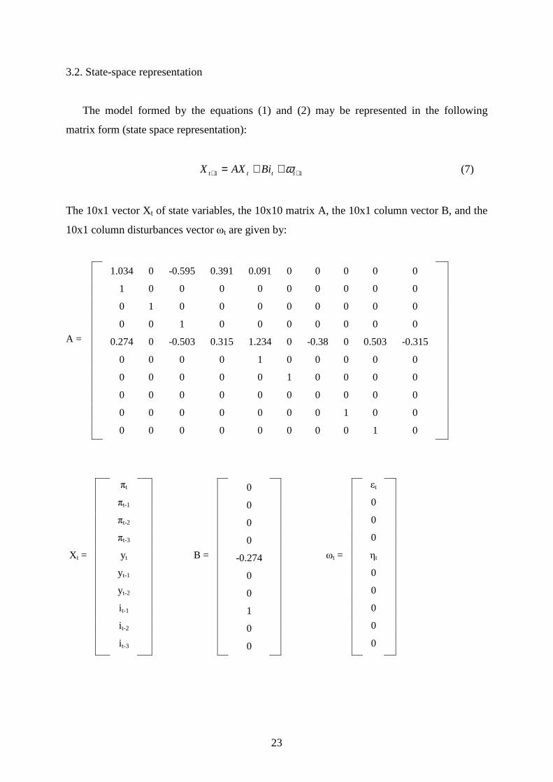
3.2. State-space representation

The model formed by the equations (1) and (2) may be represented in the following

matrix form (state space representation):

11 ++ ++= tttt BiAXX ω (7)

The 10x1 vector Xt of state variables, the 10x10 matrix A, the 10x1 column vector B, and the

10x1 column disturbances vector ωt are given by:

1.034 0 -0.595 0.391 0.091 0 0 0 0 0

1 0 0 0 0 0 0 0 0 0

0 1 0 0 0 0 0 0 0 0

0 0 1 0 0 0 0 0 0 0

A = 0.274 0 -0.503 0.315 1.234 0 -0.38 0 0.503 -0.315

0 0 0 0 1 0 0 0 0 0

0 0 0 0 0 1 0 0 0 0

0 0 0 0 0 0 0 0 0 0

0 0 0 0 0 0 0 1 0 0

0 0 0 0 0 0 0 0 1 0

πt 0 εt

πt-1 0 0

πt-2 0 0

πt-3 0 0

X t = yt B = -0.274 ωt = ηt

yt-1 0 0

yt-2 0 0

it-1 1 0

it-2 0 0

it-3 0 0

24

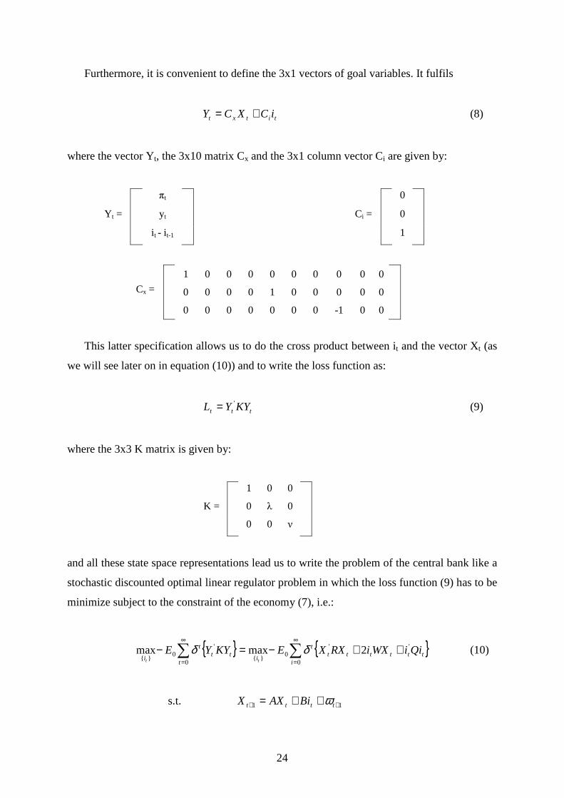
Furthermore, it is convenient to define the 3x1 vectors of goal variables. It fulfils

titxt iCXCY += (8)

where the vector Yt, the 3x10 matrix Cx and the 3x1 column vector Ci are given by:

πt 0

Yt = yt Ci = 0

it - it-1 1

1 0 0 0 0 0 0 0 0 0

Cx = 0 0 0 0 1 0 0 0 0 0

0 0 0 0 0 0 0 -1 0 0

This latter specification allows us to do the cross product between it and the vector Xt (as

we will see later on in equation (10)) and to write the loss function as:

ttt KYYL '= (9)

where the 3x3 K matrix is given by:

1 0 0

K = 0 λ 0

0 0 ν

and all these state space representations lead us to write the problem of the central bank like a

stochastic discounted optimal linear regulator problem in which the loss function (9) has to be

minimize subject to the constraint of the economy (7), i.e.:

{ } { }tttttti

t

itt

t

t

iQiiWXiRXXEKYYE

tt

''

00

}{

'

00

}{2maxmax ++−=− ∑∑

∞

=

∞

=δδ (10)

s.t. 11 ++ ++= tttt BiAXX ω

25

where

R = C'xKCx W = C'

iKCx Q = C'iKCi

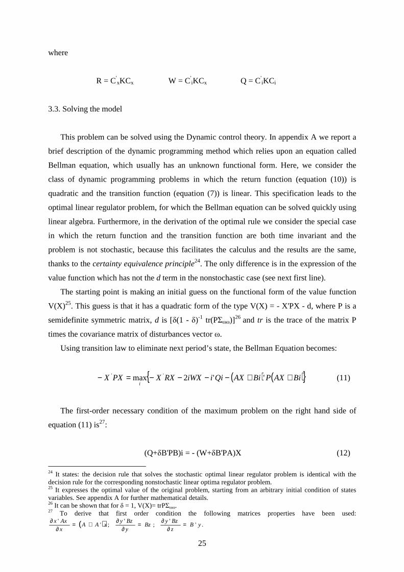
3.3. Solving the model

This problem can be solved using the Dynamic control theory. In appendix A we report a

brief description of the dynamic programming method which relies upon an equation called

Bellman equation, which usually has an unknown functional form. Here, we consider the

class of dynamic programming problems in which the return function (equation (10)) is

quadratic and the transition function (equation (7)) is linear. This specification leads to the

optimal linear regulator problem, for which the Bellman equation can be solved quickly using

linear algebra. Furthermore, in the derivation of the optimal rule we consider the special case

in which the return function and the transition function are both time invariant and the

problem is not stochastic, because this facilitates the calculus and the results are the same,

thanks to the certainty equivalence principle24. The only difference is in the expression of the

value function which has not the d term in the nonstochastic case (see next first line).

The starting point is making an initial guess on the functional form of the value function

V(X) 25. This guess is that it has a quadratic form of the type V(X) = - X'PX - d, where P is a

semidefinite symmetric matrix, d is [δ(1 - δ)-1 tr(PΣωω)]26 and tr is the trace of the matrix P

times the covariance matrix of disturbances vector ω.

Using transition law to eliminate next period’s state, the Bellman Equation becomes:

( ) ( ){ }BiAXPBiAXQiiiWXRXXPXXi

++−−−−=− ''2max '' (11)

The first-order necessary condition of the maximum problem on the right hand side of

equation (11) is27:

(Q+δB'PB)i = - (W+δB'PA)X (12)

24 It states: the decision rule that solves the stochastic optimal linear regulator problem is identical with the decision rule for the corresponding nonstochastic linear optima regulator problem. 25 It expresses the optimal value of the original problem, starting from an arbitrary initial condition of states variables. See appendix A for further mathematical details. 26 It can be shown that for δ = 1, V(X)= trPΣωω. 27 To derive that first order condition the following matrices properties have been used:

( ) .''

;'

;''

yBz

BzyBz

y

BzyxAA

x

Axx =∂

∂=∂

∂+=∂

∂

26

which implies a rule of the type:

i = FX (13)

where F = -inv(Q+δB'PB)(W+δB'PA) and it is a 1x10 vector which contains the optimal

response coefficient of the interest rate to each element of the vector X.

Substituting the optimizer (13) into the right hand side of (11) and rearranging gives:

P=R+δA'PA-(W'+δA'PB)(inv(Q+δB'PB))(W+δB'PA) (14)

This equation is called the algebraic matrix Riccati equation. Under particular condition, it

has a unique positive semidefinite solution28, which is approached in the limit as j → ∞ by

iteration on the following matrix Riccati difference equation:

Pt+j=R+δA'PjA-(W'+δA'PjB)(inv(Q+δB'PjB))(W+δB'PjA) (15)

starting from P0 = 0.

The results of optimal rule under different weights (K matrices) are reported in the

following table:

Table 7. DIFFERENT VECTORS F

Λ 0.1 0.1 0.5 0.5 1 1 5 5 100 100

Ν 0.01 0.1 0.01 0.1 0.01 0.1 0.01 0.1 0.01 0.1

πt 2.3377 1.0332 1.5148 0.9875 1.2925 0.9786 1.0659 0.9826 1.0034 0.9984

πt-1 -1.1794 -0.5542 -0.7893 -0.5774 -0.6938 -0.5750 -0.6015 -0.5673 -0.5770 -0.5746

πt-2 -1.0859 -0.5210 -0.9932 -0.6970 -0.9619 -0.7734 -0.9266 -0.8791 -0.9162 -0.9138

πt-3 1.6757 0.8511 1.0917 0.8207 0.9377 0.7995 0.7811 0.7577 0.7380 0.7370

yt 2.6713 1.4622 2.9124 2.0163 2.9814 2.2971 3.0550 2.8027 3.0760 3.0595

yt-1 -0.3496 -0.3312 -0.3296 -0.3568 -0.3228 -0.3556 -0.3150 -0.3338 -0.3126 -0.3140

yt-2 -0.7434 -0.4703 -0.8290 -0.6200 -0.8534 -0.6918 -0.8795 -0.8183 -0.8870 -0.8829

i t-1 0.6802 0.8026 0.6209 0.7510 0.6024 0.7143 0.5820 0.6308 0.5760 0.5794

i t-2 0.6942 0.3480 0.8240 0.5249 0.8620 0.6210 0.9031 0.8065 0.9150 0.9084

i t-2 -0.6162 -0.3899 -0.6872 -0.5139 -0.7074 -0.5735 -0.7291 -0.6783 -0.7353 -0.7319

28 Having eigenvalues in A of modulus less than unity is a sufficient condition.

27

The numerical values associated with the weights have not a particular meaning by their

own. What it is important is the relative weight between objectives. For instance, since the

weight on inflation is always 1, a weight of 0.1 on the output gap objective means that the

Central Bank puts one tenth of weight on it with respect to inflation stabilization. A weight of

5 implies that output stabilization is five times more important that inflation stabilization, and

so on. Moreover, a weight of 0.01 is like to say zero importance of that target, and 0.1 for

output can be considered a quasi-strict inflation targeting regime, which we here consider as

strict.

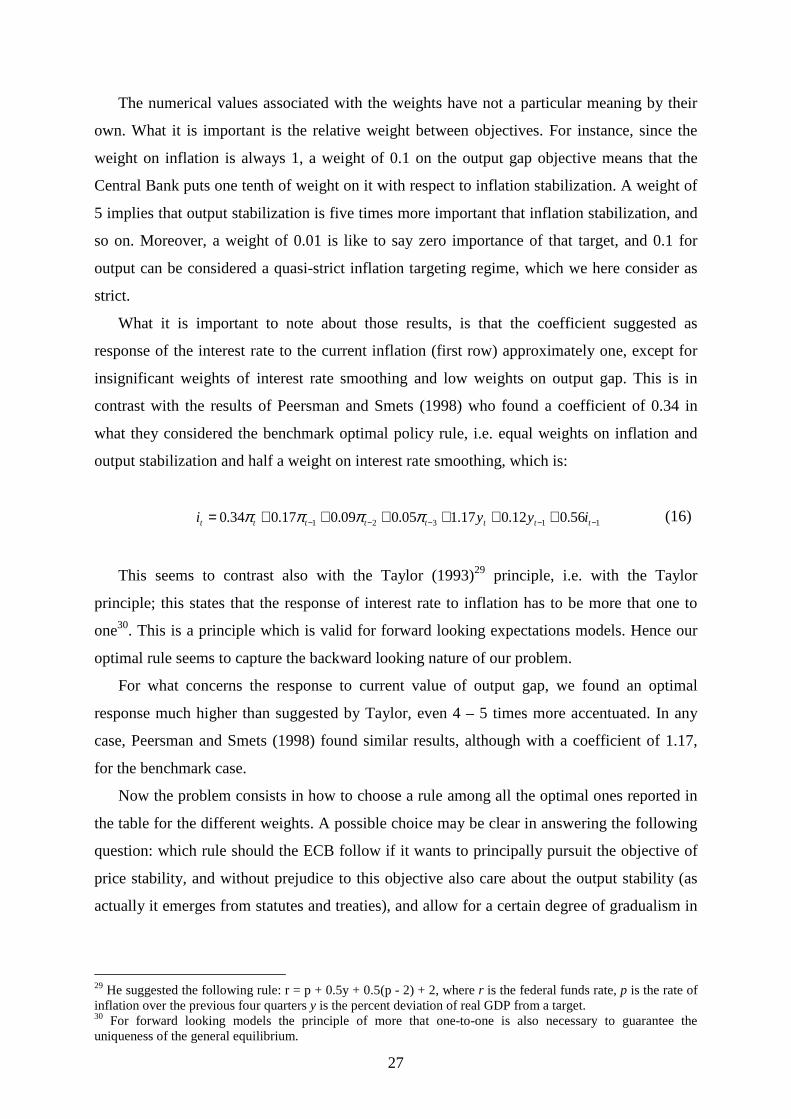
What it is important to note about those results, is that the coefficient suggested as

response of the interest rate to the current inflation (first row) approximately one, except for

insignificant weights of interest rate smoothing and low weights on output gap. This is in

contrast with the results of Peersman and Smets (1998) who found a coefficient of 0.34 in

what they considered the benchmark optimal policy rule, i.e. equal weights on inflation and

output stabilization and half a weight on interest rate smoothing, which is:

11321 56.012.017.105.009.017.034.0 −−−−− ++++++= tttttttt iyyi ππππ (16)

This seems to contrast also with the Taylor (1993)29 principle, i.e. with the Taylor

principle; this states that the response of interest rate to inflation has to be more that one to

one30. This is a principle which is valid for forward looking expectations models. Hence our

optimal rule seems to capture the backward looking nature of our problem.

For what concerns the response to current value of output gap, we found an optimal

response much higher than suggested by Taylor, even 4 – 5 times more accentuated. In any

case, Peersman and Smets (1998) found similar results, although with a coefficient of 1.17,

for the benchmark case.

Now the problem consists in how to choose a rule among all the optimal ones reported in

the table for the different weights. A possible choice may be clear in answering the following

question: which rule should the ECB follow if it wants to principally pursuit the objective of

price stability, and without prejudice to this objective also care about the output stability (as

actually it emerges from statutes and treaties), and allow for a certain degree of gradualism in

29 He suggested the following rule: r = p + 0.5y + 0.5(p - 2) + 2, where r is the federal funds rate, p is the rate of inflation over the previous four quarters y is the percent deviation of real GDP from a target. 30 For forward looking models the principle of more that one-to-one is also necessary to guarantee the uniqueness of the general equilibrium.

28

the monetary policy (as it merges from its experience31)? In order to reach all those objective

the weights that have to be chose are λ = 1 and ν = 0.1, or in other words the ECB has to set

the interest rate according with the following rule (forth column of table 7):

32121321 51.052.075.062.036.002.282.07.058.098.0 −−−−−−−− −++−−++−−= ttttttttttt iiiyyyi ππππ (17)

A first observation is worth making. As we already said, our optimal rule implies a

response of approximately one-to-one current inflation. This is the main result of my analysis.

Since the economic features of the euro area have changed a lot in the last years, also the

policy suggestions have changed accordingly. In fact, using the same argument of Peersman

and Smets (1998), if the inflation is less persistent as in our case, this may be interpreted as

higher credibility of the inflation target and this implies in turn that the central bank will need

to lean relatively less against inflation.

Secondly, we found that the coefficient on current value of output gap is higher than both

the coefficient on inflation and of the Taylor rule suggestion. From the literature it is not clear

as for the inflation which has to be the right magnitude of the coefficient on output gap, but

our result is for instance in line Peersman and Smets (1998). This may be explained by the

relative low importance of it in the role to stabilize inflation implied by our model.

Moreover, we can note that the coefficient on the first lag of interest rate in equation (17)

is equal to 0.75, suggesting a high persistence, i.e. a high propensity for ECB to smooth the

interest rate. In some cases (e.g. in Peersman and Smeets (1998)), this may reflect the fact that

the weight put in the loss function on interest rate smoothing is high, but in our case we obtain

similar results in terms of persistence even if we put very low weight on it, as it is possible to

note looking at the eighth row of table 7, in which responses of i t to i t-1 are in the range of

0.5760 – 0.6802 when ν = 0.01.

Finally, another important analysis regarding the short run concerns the relationship

between the coefficients on inflation and output gap when one of them changes, given a

certain weight on interest rate smoothing. This relation is easily viewable in figure 10; for the

short run rule, it shows the relationship between the change in the optimal response

coefficient of interest rate to the current value of inflation and output gap, given a certain

weight on interest rate smoothing, i.e. the first and fifth row of table 7 above.

31 For the interest rate smoothing preferences of ECB see Miguel C. (2006).

29

Fig. 10. EFFICIENT OPTIMAL FEEDBACK RULE COEFFICIEN TS RELATIONSHIP

For ν = 0.01, an increase in the output gap weight even very small requires a very big

variation in the coefficient of inflation to allow for the policy rule to be still optimal.

Contrary, with a bigger weight on interest rate smoothing (ν = 0.1), which is the case for the

ECB, the relation reverts, i.e. whatever the weight on the output gap, it is always optimal to

respond one-to-one to current inflation.

30

4. ANALISYS OF THE OPTIMAL RULE

4.1 Efficiency Frontier

In the previous paragraph we have derived the formula to compute the vector F of the

optimal responses of interest rate to the state and goals variables and their lags. Now, for any

given optimal vector we can compute the numerical value of the loss experimented by the

Central bank associated with that particular rule.

The following computation is necessary for the derivation of the loss. Hence, for any

vector F, the dynamic of the model follows32:

Xt+1 = MXt + ωt+1 (18)

Yt = CXt (19)

where the matrices M and C are given by

M = A + BF (20)

C = Cx + CiF (21)

Moreover, looking at the equation (5), we can see that when δ → 1 the sum in that

equation becomes unbounded. It consists in two components, however, one corresponding to

the deterministic optimization problem when all shocks are zero, and one proportional to the

variance of the shocks33. The former component converges for δ = 1 (because the terms

approach zero quickly enough), and the decision problem is actually well defined also for that

case. For δ → 1, the value of the intertemporal loss function approaches the infinite sum of

unconditional means of the period loss function, E[Lt]. Then, the scaled loss function

( ) ∑∞

= +−0

1r rt

rt LE δδ approaches the unconditional mean E[Lt]. It follows that we can also

define the optimization problem for δ = 1 (which we assume in the following analysis, on the

basis of the fact that in the literature a value of δ equal to 0.99 is usually assumed) and then

interpret the intertemporal loss function as the unconditional mean of the period loss function,

which equals the weighted sum of the unconditional variances of the goal variables:

32 It is obtained with simple substitution of equation 14 into equations 8 and 9 respectively. 33 It is possible to demonstrate that E[Lt] = trace (KΣωω).

31

E[Lt] = Var[πt] + λVar[yt] + νVar[i t – it-1] (22)

In the end, for any given rule F that results in finite unconditional variances of the goal

variables, the unconditional loss fulfils:

E[Lt] = E[Yt'KY t] = trace(KΣYY) (23)

where ΣYY is the unconditional covariance matrix of the goal variables (see appendix B).

The following table presents the values of the loss function and the standard deviation of

inflation and output stabilization computed as explained above:

Table 8. VARIANCES AND LOSS VALUES

ν=0.01 ν=0.1 λ σπ σy σr L σπ σy σr L

0.1 0.12033 0.13313 0.87346 0.14238 0.13523 0.17921 0.32302 0.18645 0.3 0.12598 0.10306 0.83486 0.16525 0.13537 0.12865 0.41809 0.21577 0.5 0.12869 0.09616 0.83461 0.18512 0.13545 0.11314 0.47591 0.23962 0.7 0.13027 0.09350 0.83821 0.20411 0.13558 0.10589 0.51666 0.26137 1 0.13169 0.09177 0.84353 0.23190 0.13573 0.10033 0.56078 0.29214 2 0.13368 0.09027 0.85418 0.32277 0.13598 0.09400 0.64466 0.38846 3 0.13445 0.08995 0.85924 0.41289 0.13607 0.09209 0.68982 0.48134 5 0.13510 0.08977 0.86400 0.59261 0.13613 0.09076 0.73988 0.66396 10 0.13562 0.08969 0.86806 1.04126 0.13616 0.09000 0.79261 1.11545 100 0.13612 0.08967 0.87211 9.11197 0.13617 0.08967 0.86255 9.18952

Taylor• 0.18197 0.53847 0.15122 0.46633 P&S1•• 0.15227 0.26270 0.36890 0.32051 P&S2••• 0.15020 0.22089 0.25097 0.28574 The loss values of all the special cases (except the pure inflation target case) reported in the table are computed imposing λ=0.5 and ν=0.1. In this way, I can measure the loss experimented by the ECB in following a rule different from what its preferences are (or should be). P&S = Peesrman and Smets (1998). The column with the loss value function (L) is obtained by σπ+λσy+νσr. • Taylor values are obtained by imposing restrictions on the elements of the vector F, i.e. imposing that all the elements are zero except the first (f1) equal to 1.5 and the fifth (f5) equal to 0.5. •• Obtained imposing f1=1.53 and f5=1.58. ••• Obtained imposing equation (16).

In the first place, we can note that the total loss corresponding to the case ν = 0.01 is

always less than the case of ν = 0.1. However, this does not seem a good reason to choose the

first alternative. In fact, bearing in mind the sense of my exercise, I am searching what it is

optimal for the ECB if it wants to principally care about inflation, but also about output

stability and interest rate smoothing.

However, what we suggested as the optimal rule for ECB (equation (17)) shows a total

loss equal to 0.23962, which is better of the most part of the remaining cases. In particular, it

32

is even better than the Taylor rule which implies an increase in the loss of about 95 per cent

with respect to the optimal rule.

In order to compare my rule with the rules derived by Peersman and Smets I should

compute as they do the restricted rules. Nevertheless, it is more convenient to calculate the

loss implied by their rules (last two rows of table 8) and compare it with the loss implied by

my rule. As it is clear, both of them are worst than mine.

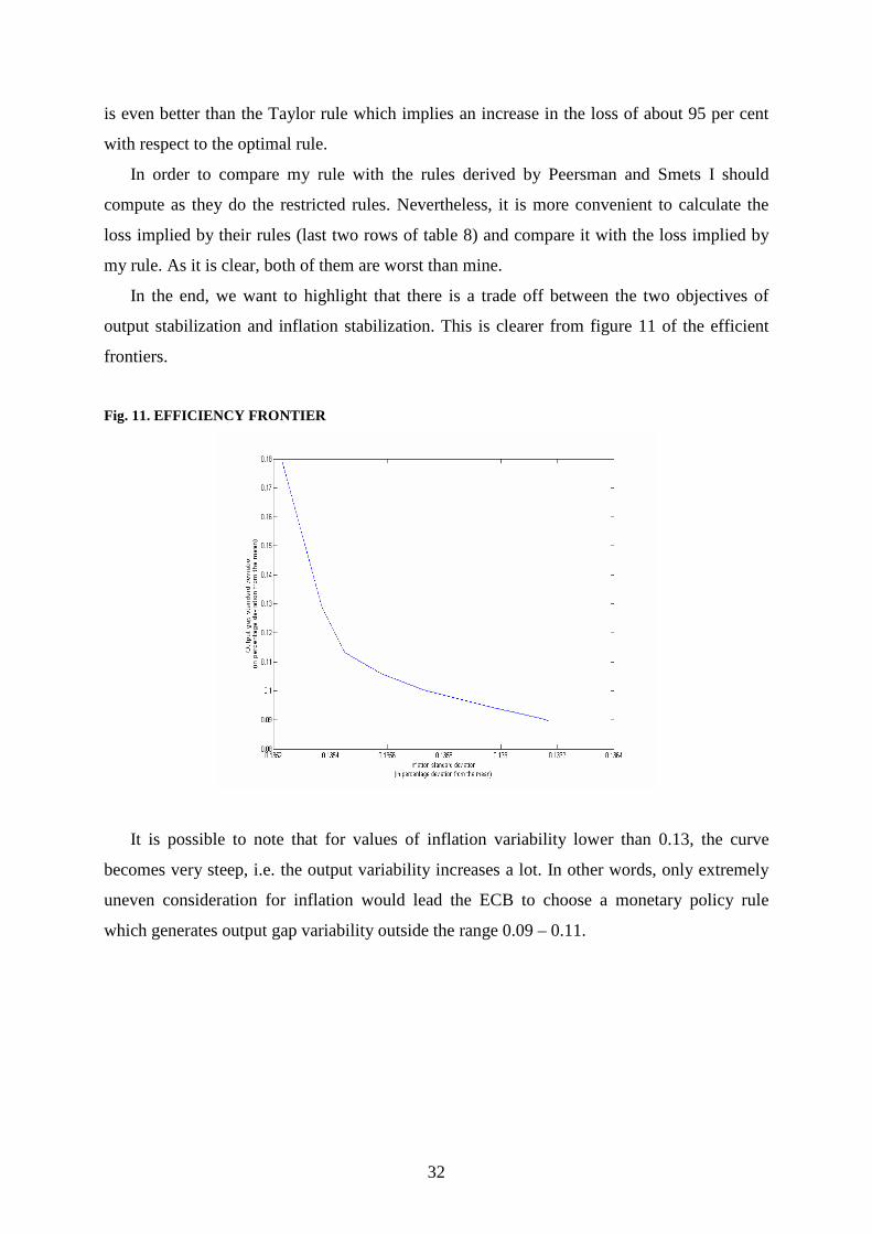
In the end, we want to highlight that there is a trade off between the two objectives of

output stabilization and inflation stabilization. This is clearer from figure 11 of the efficient

frontiers.

Fig. 11. EFFICIENCY FRONTIER

It is possible to note that for values of inflation variability lower than 0.13, the curve

becomes very steep, i.e. the output variability increases a lot. In other words, only extremely

uneven consideration for inflation would lead the ECB to choose a monetary policy rule

which generates output gap variability outside the range 0.09 – 0.11.

33

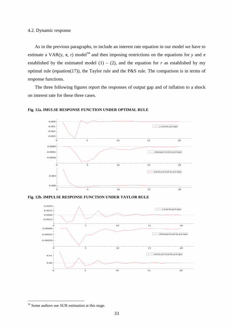
4.2. Dynamic response

As in the previous paragraphs, to include an interest rate equation in our model we have to

estimate a VAR(y, π, r) model34 and then imposing restrictions on the equations for y and π

established by the estimated model (1) – (2), and the equation for r as established by my

optimal rule (equation(17)), the Taylor rule and the P&S rule. The comparison is in terms of

response functions.

The three following figures report the responses of output gap and of inflation to a shock

on interest rate for these three cases.

Fig. 12a. IMULSE RESPONSE FUNCTION UNDER OPTIMAL RULE

0 5 10 15 20

-0.003

-0.002

-0.001

0.000

y (real int pcd eqn)

0 5 10 15 20

-0.0004

-0.0002

0.0000

infanrapcd (real int pcd eqn)

0 5 10 15 20

0.000

0.005

real int pcd (real int pcd eqn)

Fig. 12b. IMPULSE RESPONSE FUNCTION UNDER TAYLOR RULE

0 5 10 15 20

-0.0025

0.0000

0.0025

0.0050

y (real int pcd eqn)

0 5 10 15 20

-0.00050

-0.00025

0.00000

infanrapcd (real int pcd eqn)

0 5 10 15 20

0.00

0.01real int pcd (real int pcd eqn)

34 Some authors use SUR estimation at this stage.

34

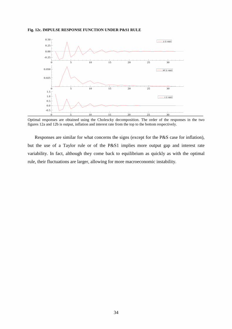
Fig. 12c. IMPULSE RESPONSE FUNCTION UNDER P&S1 RULE

0 5 10 15 20 25 30

-0.25

0.00

0.25

0.50y (r eqn)

0 5 10 15 20 25 30

0.025

0.050 inf (r eqn)

0 5 10 15 20 25 30

-0.5

0.0

0.5

1.0

1.5

r (r eqn)

Optimal responses are obtained using the Cholescky decomposition. The order of the responses in the two figures 12a and 12b is output, inflation and interest rate from the top to the bottom respectively.

Responses are similar for what concerns the signs (except for the P&S case for inflation),

but the use of a Taylor rule or of the P&S1 implies more output gap and interest rate

variability. In fact, although they come back to equilibrium as quickly as with the optimal

rule, their fluctuations are larger, allowing for more macroeconomic instability.

35

CONCLUSIONS

I started my work with the question: "does it make sense to do monetary policy analysis

with respect to a Central Bank taking into account a period in which that Central Bank does

not exist?”, and the answer I anticipated was “it probably does not”.

After my analysis, I can affirm that the answer is “it does not”, especially for the

European central bank and the Euro Area. The main reason is because the features of the euro

area have changed in the last years (in terms principally of less persistence in the inflation

process) and the policy implications of those changes are quite important.

In particular, we found that the coefficient suggested as response of the interest rate to the

current inflation is smaller then what indicated by Taylor (1993). This contrasts with results

of Peersman and Smets (1998) who found an even smaller coefficient.

Our results seem to contrast also with the Taylor principle, i.e. that the response of interest

rate to inflation has to be more that one to one. This is a principle which is valid for forward

looking expectations models. Hence our optimal rule seems to capture the backward looking

nature of our problem.

As a general conclusion then, contrary to what suggested by Taylor (1999b), who

suggested that “[a] clear guideline, or policy rule [referring to his rule], for ECB decisions

would go a long way toward reducing uncertainty and increasing economic stability

throughout the globe”, and by Peersman and Smets (1998) who argued that “… it may be

worth considering a simple guideline like the one suggested by Taylor (1993) as a benchmark

for analysing monetary policy in the euro area”, ECB should not follow any Taylor rule, but

rather the optimal rule we derived here, if the model we estimated is a reasonably good

approximation of the way the euro area works. In fact, the adoption of theTaylor rule would

imply an increase in the loss of the ECB of about 95 per cent. Other form of suggested rule,

for instance those suggested by Peersman and Smets (1998), again imply a higher loss.

As for the interest rate smoothing, we found that it is optimal for the ECB to allow for a

high degree of policy gradualism or interest rate smoothing, since the coefficient of the first

lag of interests rate in the rule is 0.75. This result is not affected by the weight put on policy

inertia in the loss function.

In the end, as concerns the response to the current value of output gap, we found that such

a coefficient is higher than both the coefficient on inflation and the Taylor rule suggestion.

From the literature, it is not clear, as for the inflation, which has to be the right magnitude of

the coefficient on output gap, but our result is for instance in line Peersman and Smets (1998).

36

This may be explained by the relative low importance of it in the role to stabilize inflation

implied by our model.

In any case, however, we found what other found in the recent literature on the estimation

of policy rules for ECB regarding the period after 1999, i.e. that the ECB appears to react

strongly to movements in real economic activity, or, as (Neumann, 2001, p. 14) puts it, “…

ECB’s monetary policy is not just guided by the price stability objective but to a considerable

degree also tries to stabilise the business cycle.”

Another interesting result is that a trade off between the two objectives of output

stabilization and inflation stabilization emerges. We can remember that for values of inflation

variability lower than 0.13, the curve becomes very steep, i.e. the output variability increases

a lot. In other words, only extremely uneven consideration for inflation would lead the ECB

to choose a monetary policy rule which generates output gap variability outside the range 0.09

– 0.11.

In the end, we want to conclude with some suggestions for further research, that we could

not pursue here since the addition of other regressors in equation(1) – (2) would have implied

too few degrees of freedom. In particular we could specify a bigger and more complex model

of the European economy, including for example the open economy aspects, and hence

allowing for the effects of exchange rate; or more include the financial sector, considering

financial variables such as stock prices. Those last variables may be also considered as good

variables to be inserted in the objective function, because the necessity for a central bank to

target the financial variables is still an open issue.

Nevertheless, the most important modification is to allow for asymmetries in the objective

function. In fact, it is not clear why the central bank should experiment the same loss for the

negative and the positive deviation of the variables from their targets.

37

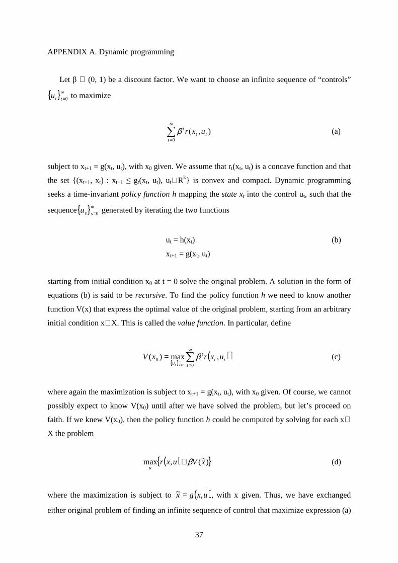
APPENDIX A. Dynamic programming

Let β ∈ (0, 1) be a discount factor. We want to choose an infinite sequence of “controls”

{ }∞=0ttu to maximize

),(0

ttt

t uxr∑∞

=β (a)

subject to xt+1 = g(xt, ut), with x0 given. We assume that rt(xt, ut) is a concave function and that

the set {(xt+1, xt) : xt+1 ≤ gt(xt, ut), ut∈Rk} is convex and compact. Dynamic programming

seeks a time-invariant policy function h mapping the state xt into the control ut, such that the

sequence{ }∞=0ssu generated by iterating the two functions

ut = h(xt) (b)

xt+1 = g(xt, ut)

starting from initial condition x0 at t = 0 solve the original problem. A solution in the form of

equations (b) is said to be recursive. To find the policy function h we need to know another

function V(x) that express the optimal value of the original problem, starting from an arbitrary

initial condition x∈X. This is called the value function. In particular, define

{ }( )∑

∞

=∞

=

=0

0 ,max)(0 t

ttt

uuxrxV

ss

β (c)

where again the maximization is subject to xt+1 = g(xt, ut), with x0 given. Of course, we cannot

possibly expect to know V(x0) until after we have solved the problem, but let’s proceed on

faith. If we knew V(x0), then the policy function h could be computed by solving for each x∈

X the problem

( ){ })~(,max xVuxru

β+ (d)

where the maximization is subject to ( )uxgx ,~ = , with x given. Thus, we have exchanged

either original problem of finding an infinite sequence of control that maximize expression (a)

38

for the problem of finding the optimal value function V(x) and a function h that solves the

continuum of maximization problems (d) – one maximum problem for each value of x. This

exchange doesn’t look like a progress, but we shall see that it often is.

Out task has become jointly to solve for V(x), h(x), which are linked by the Bellman

equation

( ) ( ) ( )[ ]{ }uxgVuxrxVu

,,max β+= (e)

The maximize of the right hand side of equation (e) is a policy function h(x) that satisfies

V(x) = r[x, h(x)] + βV{g[x, h(x)]} (f)

Equation (e) or (f) is a functional equation to be solved for the pair of unknown function

V(x), h(x).

Methods for solving the Bellman equation are based on mathematical structures that vary

in their details depending on the precise nature of the functions r and g, but the description of

those methods goes beyond the scope of this appendix, hence we will refer to Ljungqvist and

Sargent (2004).

39

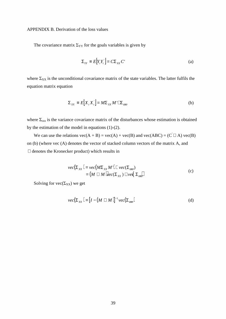
APPENDIX B. Derivation of the loss values

The covariance matrix ΣYY for the goals variables is given by

[ ] '' CCYYE XXttYY Σ=≡Σ (a)

where ΣXX is the unconditional covariance matrix of the state variables. The latter fulfils the

equation matrix equation

[ ] ωωΣ+Σ=≡Σ '' MMXXE XXttXX (b)

where Σωω is the variance covariance matrix of the disturbances whose estimation is obtained

by the estimation of the model in equations (1)-(2).

We can use the relations vec(A + B) = vec(A) + vec(B) and vec(ABC) = (C' ⊗ A) vec(B)

on (b) (where vec (A) denotes the vector of stacked column vectors of the matrix A, and

⊗ denotes the Kronecker product) which results in

( ) ( )( ) ( )ωω

ωω

Σ+Σ⊗=Σ+Σ=ΣvecvecMM

vecMMvecvec

XX

XXXX

)(

)(' (c)

Solving for vec(ΣXX) we get

( ) ( )[ ] ( )ωωΣ⊗−=Σ − vecMMIvec XX1 (d)

40

REFERENCES Adalid, A., Günter, C., McAdam, P., Siviero, S. (2005), The Performance and Robustness of

Interest-Rate Rules in Model of Euro Area, ECB’s Working Paper No. 479. Angelini, P., Del Giovane, P., Siviero, S. and Terlizzese, D. (2002), Monetary Policy Rules

for the Euro Area: What Role for National Information?, Temi di discussione, Banca d’Italia.

Angeloni, I., Aucremanne, L., Ehrmann, M., Gali, J., Levin, A., Smets, F. (2005), Inflation

Persistence in the Euro Area: Preliminary Summary of Findings, drafted for the Inflation Persistence Network.

Ball, L. (1999), Policy Rules for Open Economies, in John B. Taylor, ed., Monetary Policy

Rules. Chicago, Illinois: University of Chicago Press, 127-144. Bank for International Settlements (1995), Financial Structure and the Monetary Policy

Transmission Mechanism, Basle, Switzerland. Bofim, A. N. and Rudebusch, G. D. (1997), Opportunistic and Deliberate Disinflation Under

Imperfect Credibility, Federal Reserve Bank of San Francesco. Breuss, F. (2002), Was ECB’s monetary policy optimal?, Atlantic EconomicJournal, 30, 298-

320. Bryant, R. C., Hooper P. and Mann C., eds., (1993), Evaluating Policy Regimes: New

Research in Empirical Macroeconomics, Brooking Institute, Washington, DC. Casares, M. (2006), ECB Interest-Rate Smoothing, International Economic Trends, Federal

Reserve Bank of ST. Louis. Castelnuovo, E. and Surico, P. (2004), Model Uncertainty, Optimal Monetary Policy and the

Preferences of the Fed, Scottish Journal of Political Economy, 51(1), 105-126. Chow, G. C. (1975), Analysis and Control of Dynamic Economic Systems, John Wiley &

Sons, New York. Clarida, R., Gali, J., Gerlter, M. (1999), The Science of Monetary Policy: A New Keynesian

Perspective, NBER Working Paper. Clarida, R., Gali, J., Gerlter, M. (2000), Monetary Policy Rules and Macroeconomic Stability:

Evidence and Some Theory, The Quarterly Journal of Economic. Clausen, V. and Hayo, B. (2002), Monetary Policy in the Euro Area – Lesson from the First

Five Years, Center for European Integration Studies Working Paper. Coenen, G. and Wieland, V. (2000), A Small Estimated Euro Area Model with Rational

Expectations and Nominal Rigidities, ECB Working Paper No. 30.

41

Collard, F., Fève, P. and Langot, F. (2002), Structural Inference and the Lucas Critique”. Annales d’Economie et de Statistiques, 67/68, 183-2002.

Dieppe, A., Küster, K. and McAdam, P. (2004), Optimal Monetary Policy Rules for the Euro

Area: An Analysis Using the Area Wide Model, ECB Working Paper No. 360. Divino, J. A. C. A. and Pinto de Andrade, J. (2001), Optimal Rules For Monetary Policy In

Brazil, Paper prepared for the REDIPEA Research Network coordinated by IPEA. Engle, R. F., Hendry, D. F. and Richard, J. F. (1983), Exogeneity, Econometrica, Vol. 51, No.

2, 277-304. Estrella, A. and Fuhrer, J. C. (1999), Are ‘Deep’ Parameters Stable? The Lucas Critique as

an Empirical Testable Hypothesis, Federal Reserve Bank of Boston Working Papers, No. 99-4.

European Central Bank (2004), The Monetary Policy of the ECB. European Central Bank (October 2001), Monthly Bulletin. Fagan, G., Henry, G. and Mestre, R. (2001), An area-wide model (awm) for the Euro area,

ECB’s Working Paper No. 42. Fanelli, L. (2005), Testing the New Keynesian Phillips Curve through Vector Autoregressive

Models: Results from the Euro Area. Paper prepared for the Conference: “The Keynesian Legacy in Macroeconomic Modelling”, Cassino - Italy - 16/17 September 2005.

Fendel, R. M. and Frenkel, M. R. (2006), Five Years of Single European Monetary Policy in

Practice: Is the Ecb Rule-Based?, Contemporary Economic Policy, 24(1), 106-115. Fourçans, A. and Vranceanu, R. (2002), ECB Monetary Policy Rule: Some Theory and

Empirical Evidence, ESSEC Research Centre Working Paper No. 02008. Gali, J. (2001), European Inflation Dynamics, European Economic Review, 45, 1237-1270. Galí, J., Gerlach, S., Rotemberg, J., Uhlig, H. and Woodford, M. (2004), The monetary policy

strategy of the ECB reconsidered: Monitoring the European Central Bank 5. CEPR. Gali, J., Gerlter, M. (1999), Inflation Dynamics: a Structural Econometrics Analysis, Journal

of Monetary Economics, 44(2), 195-222. Gerdesmeier, D and Roffia, B. (2003), Empirical Estimates of Reaction Functions for the

Euro Area, ECB Working Paper No. 206. Gerlach, S. (2004), Interest Rate Retting by the EBC: Words and Deeds, CEPR Discussion

Paper 4775. Gerlach, S. and Schnabel, G. (1999), The Taylor Rule And Interest Rates in the EMU Area: A

Note, Bank for International Settlements Working Paper No. 73.

42

Goodfriend, M. and King, R. (1997), The New Neoclassical Synthesis and the role of Monetary Policy, NBER Working Paper.

Green, W. H. (2003), Econometric Analysis, 5th edition, Prentice Hall. Hansen, B. (1992), Testing for Parameter Instability in Linear Models, Journal of Policy

Modeling, 14, 517-533. Issing, O. (2003), Panel discussion at the conference “Inflation Targeting: Prospects and

Problem”, http://www.ecb.int/press/key/date/2003/html/sp031017_1.en.html. Levin, A. T. and Williams J. C. (2003), Robust Monetary Policy with Competing Reference

Models, Journal of Monetary Economics, 50, 945-975. Lindé, J. (2000), Monetary Policy Analysis in Backward-Looking Models, Central Bank of

Sweden Working Paper No. 114. Lindé, J. (2001), Testing for the Lucas Critique: a Quantitative Investigation. American

Economic Review, 91(4), 986-1005. Ljungqvist, L. and Sargent, T. J. (2004), Recursive Macroeconomic Theory, 2nd edition, MIT

Press. Lubik, T. A. and Surico, P.(2006), The Lucas Critique and the Stability of Empirical Models,

Richmond Federal Reserve Bank Working Paper. Miguel, C. (2006), ECB Interest-Rate Smoothing, International Economic Trends, Federal

Reserve Bank of St. Louis. Mishkin, F. S. (2001), Inflation Targeting, Prepared for Brian Vane and Howard Vine, An

Encyclopedia of Macroeconomics. Monacelli, T. (2006), Incomprensibile BCE, on www.lavoce.info. Monteforte, L. and Siviero, S. (2002), The Economic Consequences of Euro Area Modelling

Shortcuts, Temi di discussione, Banca d’Italia. Neumann, M. J.M. (2001), Background paper for EMU Monitor. Peersman, G. and Smets, F. (1999), Uncertainty and the Taylor rule in a simple model of the

Euro-area economy, Federal Reserve Bank of San Francesco. Peersman, G. and Smets, F. (2001), The monetary transmission mechanism in the Euro area:

more evidence from VAR analysis, ECB Working Paper No. 91. Rudebusch, G. D. and Svensson, L. E. O. (1998), Policy Rules for Inflation Targeting, NBER

Conference on Monetary Policy Rules. Rudebusch, G. D. and Svensson, L. E. O. (2000), Eurosystem Monetary Targeting: Lesson

from U.S. Data, NBER Working Paper.

43

Sack, B. (1998), Does the Fed Act Gradually? A VAR Analysis, Board of Governors of the Federal Reserve System.

Scheller, H. K. (2004), The European Central Bank, History, Role and Functions. Sims, C. (2001), A Review of Monetary Policy Rules, Journal of Economic Literature,

XXXIX, 562-566. Smets, F. and Wouters, (2002), Monetary Policy In An Estimated Stochastic Dynamic

General Equilibrium Model Of The Euro Area, Federal Reserve Bank of San Francisco. Smets, F. and Wouters, R (2003), An Estimated Stochastic Dynamic General Equilibrium

Model Of The Euro Area, ECB Working Paper No. 171. Stock, J. H. and Watson, M. W. (2001), Vector Autoregression, Journal of Economic

perspectives, 15(4), 101-115. Svensson, L. E. O. (1997), Inflation targeting: Some Extensions, NBER Woking Paper. Svensson, L. E. O. (2000), Open-Economy Inflation Targeting, Journal of International

Economics, 50 (1), 155-183. Taylor, J. B. (), The Role of the Exchange Rate in Monetary Policy Rules, Carnegie-Rochester

Conference Series on Public Policy, 39, 195-214. Taylor, J. B. (1993), Discretion versus Policy Rules in Practice, Carnegie-Rochester

Conference Series on Public Policy, 39, 195-214. Taylor, J. B., ed., (1998), The Robustness and Efficiency of Monetary Policy Rules as

Guidelines for Interest Rate Setting by the European Central Bank, Institute for International Economic Studies, Stockholm University, Seminar Paper No. 649.

Taylor, J. B., ed., (1999a), Monetary Policy Rules, NBER and University of Chicago Press,

Chicago. Taylor, J. B., ed., (1999b), What the European Central Bank Needs to do, Hoover Digest,

No.1. Ullrich, K. (2003), A Comparison Between the Fed and the ECB: Taylor rules, Discussion

Paper No. 03-19, ZEW. Zampolli, F. (2006), Optimal Monetary Policy In A Regime-Switching Economy: The

Response To Abrupt Shifts In Exchange Rate Dynamics, Bank of England Working Paper No. 297.

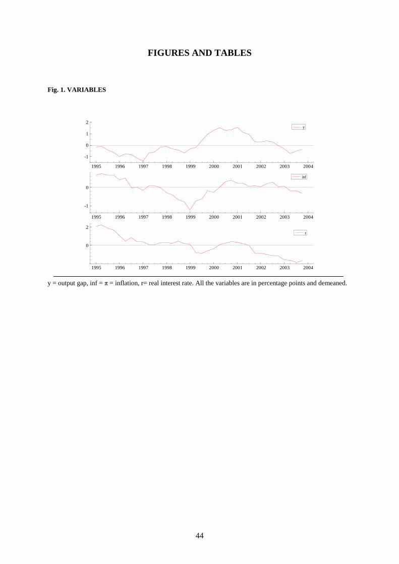
44

FIGURES AND TABLES Fig. 1. VARIABLES

1995 1996 1997 1998 1999 2000 2001 2002 2003 2004

-1

0

1

2y

1995 1996 1997 1998 1999 2000 2001 2002 2003 2004

-1

0

inf

1995 1996 1997 1998 1999 2000 2001 2002 2003 2004

0

2r

y = output gap, inf = π = inflation, r= real interest rate. All the variables are in percentage points and demeaned.

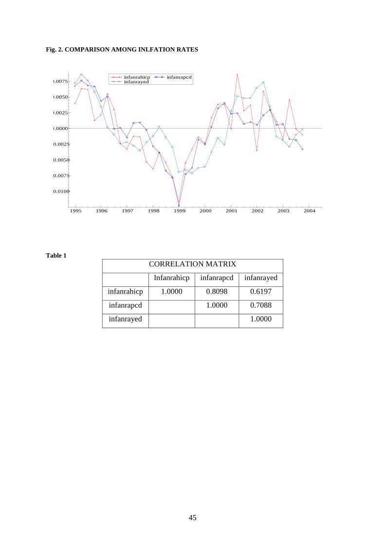
45

Fig. 2. COMPARISON AMONG INLFATION RATES

1995 1996 1997 1998 1999 2000 2001 2002 2003 2004

-0.0100

-0.0075

-0.0050

-0.0025

0.0000

0.0025

0.0050

0.0075infanrahicp infanrayed

infanrapcd

Table 1

CORRELATION MATRIX

Infanrahicp infanrapcd infanrayed

infanrahicp 1.0000 0.8098 0.6197

infanrapcd 1.0000 0.7088

infanrayed 1.0000

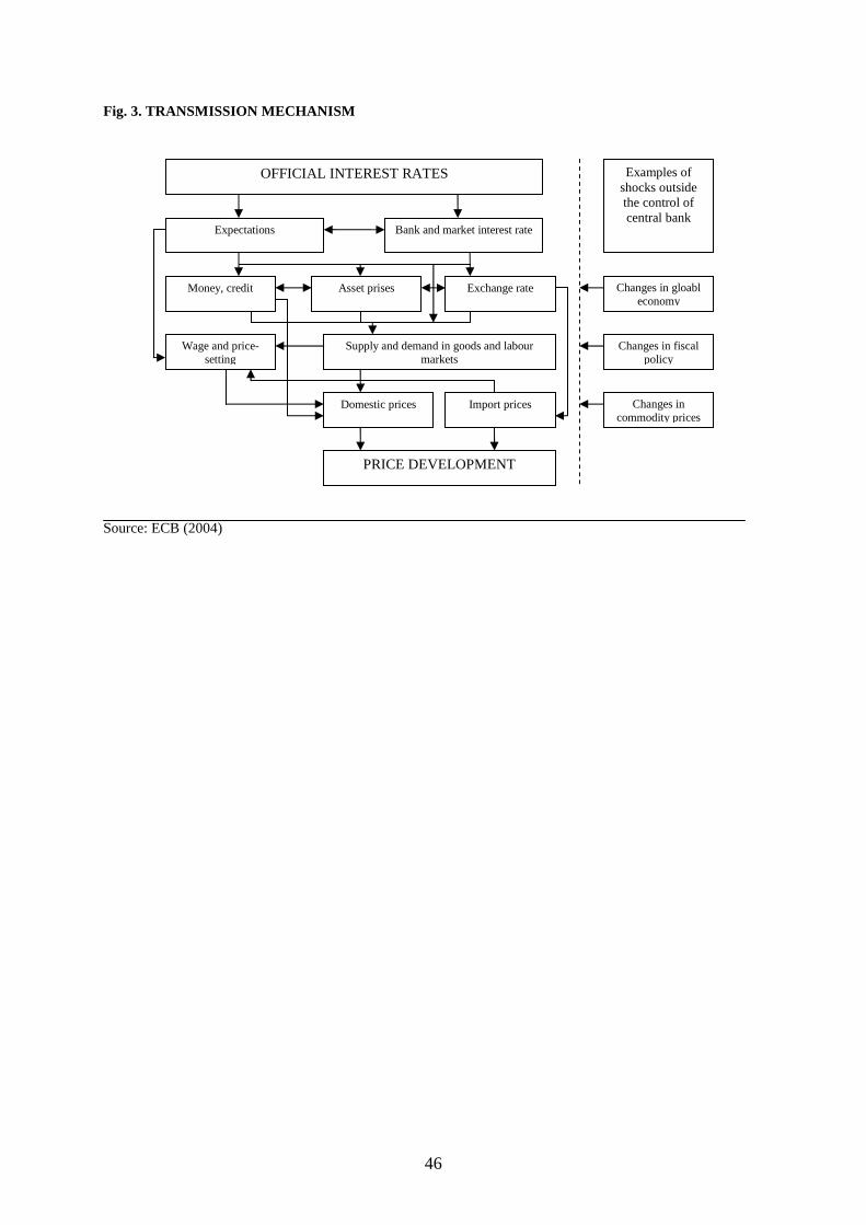
46

Fig. 3. TRANSMISSION MECHANISM

Source: ECB (2004)

OFFICIAL INTEREST RATES

Expectations Bank and market interest rate

Money, credit Asset prises Exchange rate

Wage and price-setting

Supply and demand in goods and labour markets

Domestic prices Import prices

PRICE DEVELOPMENT

Examples of shocks outside the control of central bank

Changes in gloabl economy

Changes in fiscal policy

Changes in commodity prices

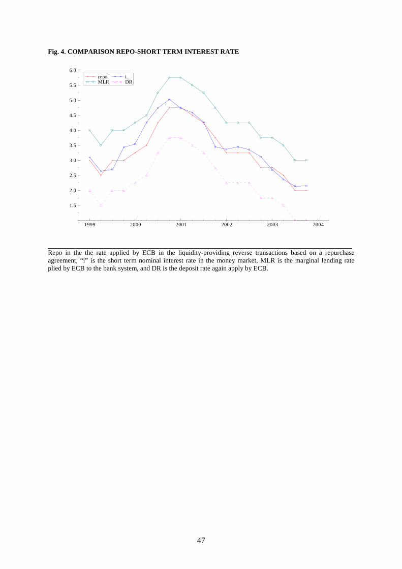
47

Fig. 4. COMPARISON REPO-SHORT TERM INTEREST RATE

1999 2000 2001 2002 2003 2004

1.5

2.0

2.5

3.0

3.5

4.0

4.5

5.0

5.5

6.0repo MLR

i_ DR

Repo in the the rate applied by ECB in the liquidity-providing reverse transactions based on a repurchase agreement, “i” is the short term nominal interest rate in the money market, MLR is the marginal lending rate plied by ECB to the bank system, and DR is the deposit rate again apply by ECB.

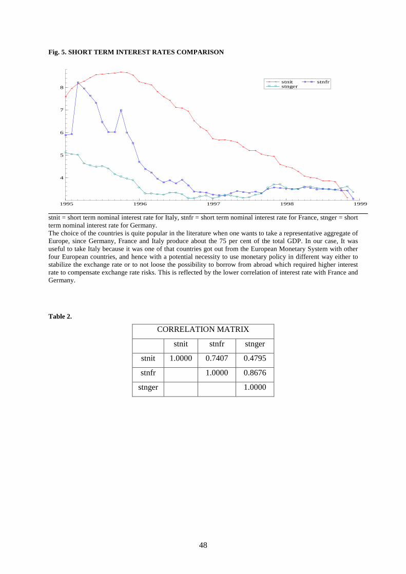
48

Fig. 5. SHORT TERM INTEREST RATES COMPARISON

1995 1996 1997 1998 1999

4

5

6

7

8stnit stnger

stnfr

stnit = short term nominal interest rate for Italy, stnfr = short term nominal interest rate for France, stnger = short term nominal interest rate for Germany. The choice of the countries is quite popular in the literature when one wants to take a representative aggregate of Europe, since Germany, France and Italy produce about the 75 per cent of the total GDP. In our case, It was useful to take Italy because it was one of that countries got out from the European Monetary System with other four European countries, and hence with a potential necessity to use monetary policy in different way either to stabilize the exchange rate or to not loose the possibility to borrow from abroad which required higher interest rate to compensate exchange rate risks. This is reflected by the lower correlation of interest rate with France and Germany.

Table 2.

CORRELATION MATRIX

stnit stnfr stnger

stnit 1.0000 0.7407 0.4795

stnfr 1.0000 0.8676

stnger 1.0000

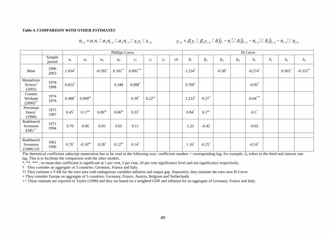
49

Table 4. COMPARISON WITH OTHER ESTIMATES

11342311 +−−+ ++++= tttttt y εγπαπαπαπ ( ) ( ) ( ) 133422312311 +−−−−−+ +−+−+−++= tttttttttt iiiyyy ηπδπδπδββ

Phillips Curve IS Curve

Sample period

α1 α2 α3 α4 γ1 γ2 γ3 γ4 β1 β2 β3 β4 δ1 δ2 δ3 δ4

Mine

1996 2003

1.034* -0.595* 0.391** 0.091*** 1.234* -0.38* -0.274* 0.503* -0.315**

Monteforte Siviero† (2002)

1978 1998

0.652* 0.348 0.088* 0.769* -0.05*

Coenen Weiland (2000)††

1974 1978

0.488* 0.099ns 0.39* 0.22ns 1.233* -0.27* -0.04***

Peersman Smets+ (1998)

1975 1997

0.45* 0.17ns 0.06ns 0.06ns 0.33* 0.84* 0.1ns -0.1*

Rudebusch Svensson EMU++

1971 1994

0.70 0.06 0.05 0.05 0.11 1.25 -0.42 -0.02

Rudebusch Svensson (1998) US

1961 1996

0.70* -0.10ns 0.28* 0.12ns 0.14* 1.16* -0.25* -0.10*

The theoretical coefficient subscript numeration has to be read in the following way: coefficient number = corresponding lag; for example, δ3 refers to the third real interest rate lag. This is to facilitate the comparison with the other models. *, **, *** , ns mean that coefficient is significant at 1 per cent, 5 per cent, 10 per cent significance level and not significance respectively. † They consider an aggregate of 3 countries: Germany, France and Italy. †† They estimate a VAR for the euro area with endogenous variables inflation and output gap. Separately, they estimate the euro area IS Curve. + They consider Europe an aggregate of 5 countries: Germany, France, Austria, Belgium and Netherlands. ++ These estimate are reported in Taylor (1998) and they are based on a weighted GDP and inflation for an aggregate of Germany, France and Italy.

50

Table 3. VARIANCES OF INFLATION AND OUTPU GAP PERIO D 1995-1998

MEAN OUTPUT GAP STANDARD DEVIATION

Germany 0 2.1851e+009

France 0 2.2681e+009

Italy 0 1.7466e+009

MEAN OUTPUT GAP STANDARD DEVIATION

Germany 0.014970 0.0045152

France 0.014041 0.0060610

Italy 0.033139 0.014912

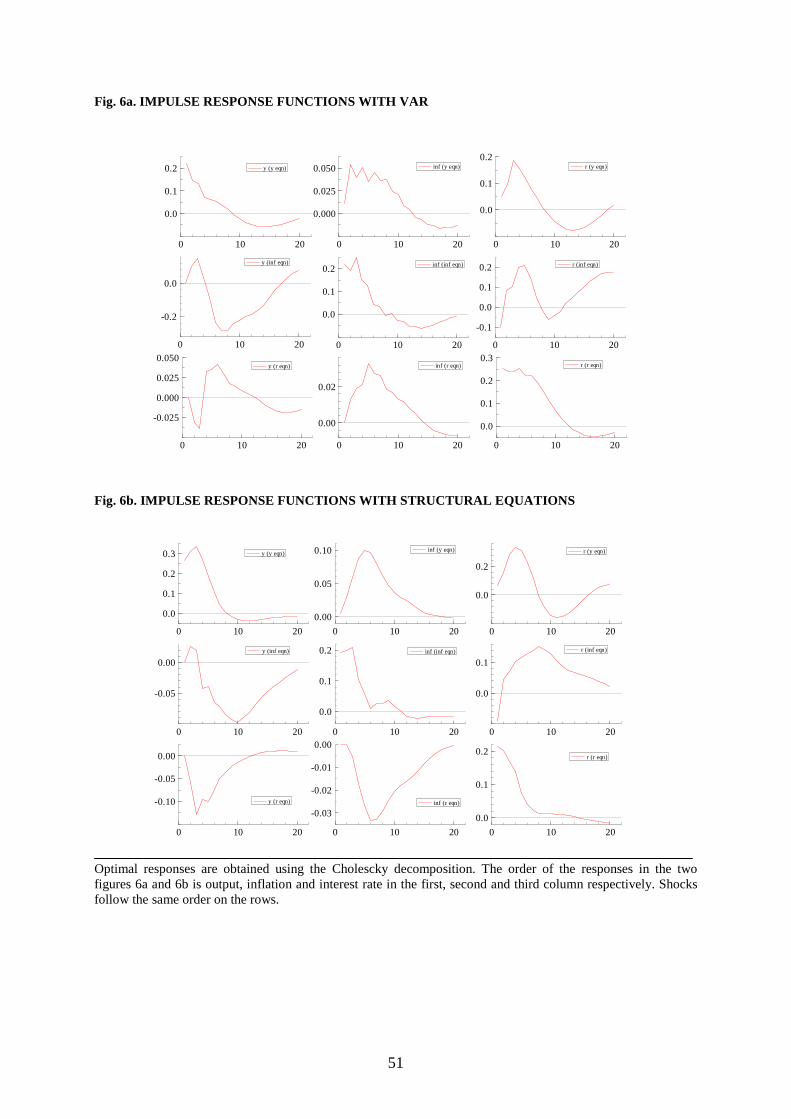
51

Fig. 6a. IMPULSE RESPONSE FUNCTIONS WITH VAR

0 10 20

0.0

0.1

0.2 y (y eqn)

0 10 20

0.000

0.025

0.050 inf (y eqn)

0 10 20

0.0

0.1

0.2r (y eqn)

0 10 20

-0.2

0.0

y (inf eqn)

0 10 20

0.0

0.1

0.2inf (inf eqn)

0 10 20

-0.1

0.0

0.1

0.2 r (inf eqn)

0 10 20

-0.025

0.000

0.025

0.050y (r eqn)

0 10 20

0.00

0.02

inf (r eqn)

0 10 20

0.0

0.1

0.2

0.3r (r eqn)

Fig. 6b. IMPULSE RESPONSE FUNCTIONS WITH STRUCTURAL EQUATIONS

0 10 20

0.0

0.1

0.2

0.3 y (y eqn)

0 10 20

0.00

0.05

0.10 inf (y eqn)

0 10 20

0.0

0.2

r (y eqn)

0 10 20

-0.05

0.00y (inf eqn)

0 10 20

0.0

0.1

0.2 inf (inf eqn)

0 10 20

0.0

0.1

r (inf eqn)

0 10 20

-0.10

-0.05

0.00

y (r eqn)

0 10 20

-0.03

-0.02

-0.01

0.00

inf (r eqn)

0 10 20

0.0

0.1

0.2r (r eqn)

Optimal responses are obtained using the Cholescky decomposition. The order of the responses in the two figures 6a and 6b is output, inflation and interest rate in the first, second and third column respectively. Shocks follow the same order on the rows.

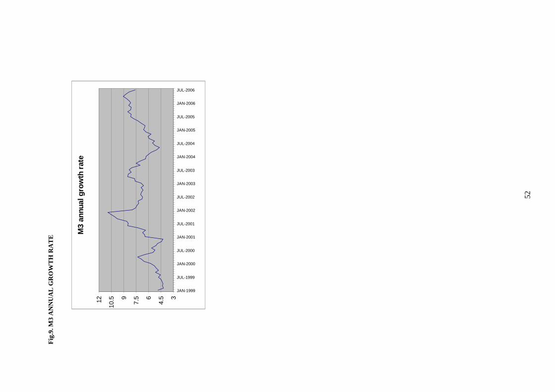
52

Fig

.9. M

3 A

NN

UA

L G

RO

WT

H R

AT

E

M3

annu

al g

row

th r

ate

3

4.56

7.59

10.512

JAN-1999

JUL-1999

JAN-2000

JUL-2000

JAN-2001

JUL-2001

JAN-2002

JUL-2002

JAN-2003

JUL-2003

JAN-2004

JUL-2004

JAN-2005

JUL-2005

JAN-2006

JUL-2006