the optimal timing of investment decisionstimj/th1.pdfabstract this thesis addresses the problem of...
TRANSCRIPT

THE OPTIMAL TIMING OFINVESTMENT DECISIONS
by
Timothy Charles Johnson.
Submitted to the University of London
for the degree of
Doctor of Philosophy.
Department of Mathematics,
King’s College London,
The Strand,
London,
WC2R 2LS.
NOVEMBER 2006

The Optimal Timing of Investment Decisions ii
I affirm that the work contained in this thesis is my own.
Timothy Charles Johnson,
November, 2006.

Abstract
This thesis addresses the problem of the optimal timing of investment decisions. A
number of models are formulated and studied. In these, an investor can enter an
investment that pays a dividend, and has the possibility to leave the investment,
either receiving or paying a fee. The objective is to maximise the expected dis-
counted cashflow resulting from the investor’s decision making over an infinite time
horizon. The initialisation and abandonment costs, the discounting factor, and the
running payoffs are all functions of a state process that is modelled by a general one-
dimensional positive Ito diffusion. Sets of sufficient conditions that lead to results of
an explicit analytic nature are identified. These models have numerous applications
in finance and economics.
To address the family of models that we study, we first solve the discretionary
stopping problem that aims at maximising the performance criterion
Ex
[e−
R τ0 r(Xs)dsg(Xτ )1τ<∞
]over all stopping times τ , where X is a general one-dimensional positive Ito diffusion,
r is a strictly positive function and g is a given payoff function. Our analysis, which
leads to results of an explicit analytic nature, is illustrated by a number of special
cases that are of interest in applications, and aspects of which have been considered
in the literature and we establish a range of results that can provide useful tools for
developing the solution to other stochastic control problems.
iii

Acknowledgements
A thesis is not the result of single persons efforts. I would not have returned to
academic study had I not had the support of Mike Smith and Brent Cheshire at
Amerada Hess. I would not have undertaken the MSc at King’s had it not been
for Mike Monoyios, who has given me enormous encouragement throughout my
studies. Lane Hughston, as chair in Financial Mathematics at King’s, has provided
an extremely supportive group. My fellow students, James, Andrea, Anne Laure,
Amal, Ovidiu and Zhengjun have all contributed, in different ways, to the thesis.
Andrew Jack has answered all my trivial questions with patience; Martijn Pistorius
has given me gentle encouragement along the way and Ian Buckley, who was in at
the inception of my studies has been a familiar face at the end. Particular mention
goes to Arne Løkka, whom I like to think has become a good friend. Beyond King’s,
I would like to acknowledge the various contributions made by, as well as Mike
Monoyios, Damien Lamberton, David Hobson, Vicky Henderson and Goran Peskir
to my understanding of the material in this thesis, and to the EPSRC, for providing
funding.
On a personal note, I would like to acknowledge the support of my family, who
have never doubted me, and friends, particularly Tony and Catherine, Hele and
Morgan, Rich and Helen, Sharon, Simon, Robert and Rachel, Doug and Shizuko,
Gwyn, Carl, Matt, Pete and Paula, Rosalind, Paul and Michelle, Tony and Lesley
and Bev and Kat.
My supervisor, Mihail Zervos, has been an exceptional support and has made
the significant contribution to my understanding of mathematics. I hope that we
will collaborate more in the future. I feel I have a great friend in Mihailis.
iv

The Optimal Timing of Investment Decisions v
Finally, I’d like to thank my lovely wife, Jo, for support, patience and belief.
Tim Johnson,
November, 2006.

Table of contents
Abstract iii
Acknowledgements iv
1 Introduction 1
2 Study of an Ordinary Differential Equation 72.1 Introduction . . . . . . . . . . . . . . . . . . . . . . . . . . . . . . . . 72.2 The properties of the underlying diffusion . . . . . . . . . . . . . . . 82.3 The solution to the homogeneous ODE . . . . . . . . . . . . . . . . . 92.4 Study of a non-homogeneous ordinary differential equation . . . . . . 17
3 A Discretionary Stopping Problem 313.1 Introduction . . . . . . . . . . . . . . . . . . . . . . . . . . . . . . . . 313.2 Problem formulation and assumptions . . . . . . . . . . . . . . . . . . 323.3 The solution to the discretionary stopping problem . . . . . . . . . . 363.4 Special cases . . . . . . . . . . . . . . . . . . . . . . . . . . . . . . . . 50
3.4.1 Geometric Brownian motion . . . . . . . . . . . . . . . . . . . 543.4.2 Square-root mean-reverting process . . . . . . . . . . . . . . . 553.4.3 Geometric Ornstein-Uhlenbeck process . . . . . . . . . . . . . 56
4 The Investment Problems 594.1 Introduction . . . . . . . . . . . . . . . . . . . . . . . . . . . . . . . . 594.2 Problem formulation and assumptions . . . . . . . . . . . . . . . . . . 604.3 The single entry or exit investment problem . . . . . . . . . . . . . . 64
4.3.1 The initialisation of a payoff flow problem . . . . . . . . . . . 644.3.2 The abandonment of a payoff flow problem . . . . . . . . . . . 664.3.3 The initialisation of a payoff flow with the option to abandon
problem . . . . . . . . . . . . . . . . . . . . . . . . . . . . . . 674.4 The sequential entry and exit investment problem . . . . . . . . . . . 72
4.4.1 The case when switching is optimal . . . . . . . . . . . . . . . 74
vi

The Optimal Timing of Investment Decisions vii
4.4.2 The case when one mode is optimal for certain values of thestate process . . . . . . . . . . . . . . . . . . . . . . . . . . . . 86
4.4.3 The case when one mode is optimal for all values of the stateprocess . . . . . . . . . . . . . . . . . . . . . . . . . . . . . . . 92

1. INTRODUCTION
We formulate and solve a number of stochastic optimisation problems that are con-
cerned with the optimal timing of investment decisions. In the course of our analysis
we investigate the solvability of an ordinary differential equation, which plays a fun-
damental role in solving the associated Hamilton-Jacobi-Bellman (HJB) equations,
and we solve a discretionary stopping problem, which is closely related to our in-
vestment models.
An investment is characterised by making a known payment in order to receive
an unknown cashflow in the future. The holder of an investment may relinquish
the cashflow once it has been initiated, for example, if the payoff of stopping is
greater than the expected value of future cashflows. A simple example could be the
decision to buy an equity, which has a transaction cost. Holding the equity gives
the investor a dividends stream. If the investor feels that the equity is undervalued,
and the current market price is less than the net present value of future dividends,
they would buy the equity. Alternatively, if the investor held the equity and it was
overvalued, they would sell it. The investor could repeat the process any number of
times. Another example could be the decision to build a production facility, which
will have a cost but will provide an income based on the demand for its product. At
some point in the future the demand for the product may fall or, equivalently, more
producers may enter the economy, and so the cashflow generated by the facility
becomes negative. At this point, the investor may be tempted to abandon the
production facility, which could incur a cost. This type of decision may be only
possible once. As the investor is under no obligation to either initiate an investment
project or to abandon an existing project, we describe the problem as discretionary.
1

The Optimal Timing of Investment Decisions 2
The motivation for the thesis came about whilst the author was working in
industry and so called “real options” models were being promoted, with the classical
real options model being that introduced by McDonald and Siegel [MS86]. The
problem considered aims to choose the stopping time τ that maximises
Ex
[(e−rτXτ −K)
].
The model addresses the question of when is it optimal to initiate an investment
project, the value of which is modelled by the state process X and initiating the
project incurs a cost K, while r is a discounting rate. This model is closely related
to the widely studied perpetual American call option, first considered by Samuel-
son [Sam65] and McKean [McK65]. When X is modelled by a geometric Brownian
motion a result of this model is that an investor in a project would either act im-
mediately, or, wait forever. This strategy is counter-intuitive to managers, whose
gut feeling tells them there are some projects that should be initialised at some
trigger level. The author was interested in whether generalising the payoff, state
process dynamics and discounting would result in more intuitive results, and how
cases where a stopping boundary, the boundary between stopping and continuation
regions, could be identified from the problem data. Another limitation of the ap-
proach taken by McDonald and Siegel was that X represents the net present value
(the discounted sum of all future cashflows) of the project. It would be preferable
to develop models that represented the whole life of the investment, of initiation,
running and abandonment. Once the partially reversible problem of initiating and
then abandoning a project is solved in a general setting, it becomes a relatively
straightforward exercise to address the reversible investment problem in a general
setting.
Models relating to single entry and exit problems have been studied in the con-
text of real options by various authors. For example, Paddock, Siegel and Smith
[PSS88] and Dixit and Pindyck [DP94, Sections 6.3, 7.1] adopt an economics per-
spective. More recent works include Knudsen, Meister and Zervos [KMZ98], who
generalise Dixit and Pindyck’s model, but consider the abandonment problem alone,

The Optimal Timing of Investment Decisions 3
and Duckworth and Zervos [DZ00], who extend Knudsen, Meister and Zervos to in-
clude the initialisation problem. In fact, the model studied by Duckworth and Zervos
[DZ00] can be seen as an extension of a fundamental real options problem introduced
by McDonald and Siegel [MS86], which is concerned with determining the value of a
firm when there is an option to shut down. McDonald and Siegel [MS86] implicitly
considered the payoff being the discounted future cashflows of the project, Knudsen,
Meister and Zervos [KMZ98] explicitly model these payoffs in solving the abandon-
ment problem, and Duckworth and Zervos [DZ00] combine the two approaches. All
these papers assume that the underlying state process is represented by a geometric
Brownian motion, and that the entry and exit costs as well as the discounting rate
are all constants.
With regard problems involving sequential entries and exits, Brekke and Øksendal
[BØ94] analyse a general model, without providing explicit results. Duckworth and
Zervos [DZ01] consider the special case where the state process is represented by a
geometric Brownian motion, the entry and exit costs as well as the discounting rate
are constants, and they provide explicit results. Other authors, such as Lumley and
Zervos [LZ01], Hodges [Hod04], Pham [Pha] and Wang [Wan05], consider related
problems.
The objective of this thesis is to study general investment models with a view to
obtaining results of an explicit nature. We consider models where the state process
driving the economy is modelled by general one-dimensional Ito diffusions, rather
than specific diffusions such as a geometric Brownian motion. We assume that
the costs associated with taking or leaving the investment and the cashflow of the
investment are deterministic functions of the state process. In addition, there is
discounting, which again may be state dependent, and the investor has an infinite
time horizon. Within this general context, we consider two investment models. In
the first one, only one entry and/or exit into the investment may be made, this is
closely related to “real options” problems were the decision is not reversible. In the
second one, any number of entries and exits can be made and is more closely related
to general investment problems. In addressing our objective, results are obtained
that are useful not only in addressing optimal stopping problems but also in solving

The Optimal Timing of Investment Decisions 4
more general stochastic control problems.
In the models we study there is some stochastic process that represents the state
of the economy, such as the price of an equity or the demand for a product. We
model this state process, X, by the one-dimensional Ito diffusion
dXt = b(Xt) dt + σ(Xt) dWt, X0 = x > 0,
where W is a standard, one-dimensional Brownian motion, and b, σ are given deter-
ministic functions such that Xt > 0, for all t > 0, with probability 1. Generalising
the existing theory so that it can account for stochastic processes modelled by gen-
eral Ito diffusions is motivated by a wide range of practical applications. These
include financial and economic applications where the assets exist in equilibrium
market conditions and tend to fluctuate about some long-term mean level, rather
than, on average, grow or fall exponentially, as modelled by a geometric Brownian
motion. Such assets include interest rates, exchange rates and commodities, where
there is empirical evidence of mean-reversion (e.g., see Metcalf and Hassett [MH95]
and Sarkar [Sar03]). Considering general Ito diffusions also facilitates modelling of
non-financial applications, such as those found in biological systems.
Introducing state dependent discounting enables a more realistic modelling frame-
work of decisions. In the context of financial decision-making, the discounting rate
accounts for the time-value of money, for the associated investment’s depreciation
rate and for the likelihood of the investment’s default. In view of this observation,
discounting should reflect the effect of the economic environment on the likelihood of
default of an investment project, which may well be related to the underlying asset’s
value or demand. Specifically, if a firm’s income relies on the price of one product,
they will find their borrowing costs higher if the price of that product falls. In a
biological setting, state dependent discounting reflects the dependence of extinction
likelihood on the environment.
State dependent payoffs are motivated by a number of applications. First, they
allow for utility based decision making, which, apart from the work of Henderson and
Hobson [HH02], and despite its fundamental importance, has hardly found its way

The Optimal Timing of Investment Decisions 5
into real options theory. Second, they allow for financial modelling based on non-
monetary state processes, for example, when the underlying process is the demand
for a product, which may be appropriate if the demand for a product can be modelled
more easily than the product’s price. Third, state-dependent payoff functions are
useful when dealing with cases where inputs are a finite resource. For example,
consider the case where a financier has decided to invest in a widget production
facility, because the price of widgets is high. In this situation, one would expect
there other financiers to be investing in other widget production facilities, and, if
widget producers are a scarce resource, their cost may go up. Within this general
framework, we identify the investment strategies that are optimal, depending on the
dynamics of the state process as well as the structure of the payoff functions and
the discounting factor.
To address the investment problems that we study, we first solve the discretionary
stopping problem that aims to maximise
Ex
[e−Λτ g(Xτ )1τ<∞
], where Λt =
∫ t
0
r(Xs)ds,
over all stopping times τ , where r is strictly positive and g is a given payoff function.
This stopping problem is related to perpetual American options whose payoff is
given by g. One of the attractive features of perpetual options is that one can
obtain explicit analytic expressions for their values and they are important in the
theory of finance because their prices provide upper bounds for the corresponding
finite maturity options. In addition, our analysis provides the prices of perpetual
American “power” options, which have been studied in discrete time by Novikov
and Shiryaev [NS04], for a range of underlying asset price dynamics.
The theory of optimal stopping has numerous applications and has attracted
the interest of numerous researchers. Important, older accounts of this theory in-
clude Shiryaev [Shi78], El-Karoui [EK79] and Krylov [Kry80] , while more recent
contributions include Salminen [Sal85], Davis and Karatzas [DK94], Øksendal and
Reikvam [ØR98], Beibel and Lerche [BL00], Guo and Shepp [GS01], Dayanik and
Karatzas [DK03] and Alvarez [Alv04]. We solve the problem that we consider by

The Optimal Timing of Investment Decisions 6
means of dynamic programming techniques, specifically we employ Bellman’s prin-
ciple to identify a variational inequality, we verify that the solution to this equation
identifies with the value function of our stopping problem and we provide a solution
to the variational inequality by appealing to the so-called smooth pasting princi-
ple. This is an approach that differs from the one taken by, for example Beibel
and Lerche [BL00], who use a martingale technique to identify the free-boundary
between the continuation and stopping region, or Dayanik and Karatzas [DK03] and
Alvarez [Alv04], who employ r-excessive functions.
In order to address our investment models in a general setting the solution of
the ODE
1
2σ2(x)w′′(x) + b(x)w′(x)− r(x)w(x) + h(x) = 0, x ∈ ]0,∞[.
needs to be understood. This understanding is developed in Chapter 2. Many of
the key results, in Section 2.4, were developed in the course of studying the discre-
tionary stopping problem presented in Chapter 3, and can be best appreciated in
hindsight. In particular, the importance of the transversality condition, introduced
in Section 3.2, in enabling explicit results to be obtained cannot be understated.
Once we have the results from Chapter 2, we solve the discretionary stopping
problem in Chapter 3. We solve this stopping problem under general assumptions
on the underlying state process X, the payoff function g and the discounting rate r.
We consider a number of special cases in Section 3.4.
The results of Chapter 3, in turn, can be applied in answering the investment
problems in Chapter 4. We presented two types of investment problems, in Sec-
tion 4.3 we addressed cases where there the structure of the problem prevents de-
cisions from being reversed, and they could all be re-cast as versions of the dis-
cretionary stopping problem studied in the preceding chapter. In Section 4.4 we
considered the case where decisions could be reversed. However, even if a decision
can be reversed, it may not be optimal to reverse a decision, and in these circum-
stances the problems reduce to the problems studied in Section 4.3.

2. STUDY OF AN ORDINARY
DIFFERENTIAL EQUATION
2.1 Introduction
In this chapter we study an ODE that plays a fundamental role in our analysis in
the following chapters. The results of this chapter have applications not only in the
field of optimal stopping but also in more general control problems.
In Section 2.4 we study the solution to the non-homogeneous ODE
1
2σ2(x)w′′(x) + b(x)w′(x)− r(x)w(x) + h(x) = 0, x ∈ ]0,∞[, (2.1)
which is related to the variational inequalities we solve in addressing our investment
models. Prior to addressing the non-homogeneous ODE we investigate the solution
to the associated homogeneous ODE in Section 2.3. In Section 2.2 we consider a
positive one-dimensional Ito diffusion that is closely related with the ODE that we
use in solving our problems in Chapters 3 and 4.
Most of the results presented here have been established by Feller [Fel52] and
can be found in various forms in several references that include Breiman [Bre68],
Mandl [Man68], Ito and McKean [IM74], Karlin and Taylor [KT81], Rogers and
Williams [RW94] and Borodin and Salminen [BS02]. Our presentation, which is
based on modern probabilistic techniques, has largely been inspired by Rogers and
Williams [RW94, Sections V.3, V.5, V.7 ] and includes ramifications not found in
the literature.
7

The Optimal Timing of Investment Decisions 8
2.2 The properties of the underlying diffusion
We consider a stochastic system, the state process X of which satisfies is modelled
by the positive, one-dimensional Ito diffusion
dXt = b(Xt) dt+ σ(Xt) dWt, X0 = x > 0, (2.2)
where W is a one-dimensional standard Brownian motion and b, σ : ]0,∞[→ R are
given deterministic functions satisfying the conditions (ND)′ and (LI)′ in Karatzas
and Shreve [KS91, Section 5.5C], and given in the following assumption.
Assumption 2.2.1 The functions b, σ : ]0,∞[→ R satisfy the following conditions:
σ2(x) > 0, for all x ∈ ]0,∞[,
for all x ∈ ]0,∞[, there exists ε > 0 such that
∫ x+ε
x−ε
1 + |b(s)|σ2(s)
ds <∞.
This assumption guarantees the existence of a unique, in the sense of probability
law, solution to (2.2) up to an explosion time. In particular, given c > 0, the scale
function pc and the speed measure mc(dx), given by
pc(x) =
∫ x
c
exp
(−2
∫ s
c
b(u)
σ2(u)du
)ds, for x > 0, (2.3)
mc(dx) =2
σ2(x)p′c(x)dx, (2.4)
are well-defined. In what follows, we assume that the constant c > 0 is fixed.
We also assume that the diffusion X is non-explosive and the boundaries of the
diffusion at zero and infinity are inaccessible. In particular, we impose the following
assumption (see Karatzas and Shreve [KS91, Theorem 5.5.29]).
Assumption 2.2.2 If we define
uc(x) =
∫ x
c
[pc(x)− pc(y)
]mc(dy), (2.5)
then limx↓0 uc(x) = limx→∞ uc(x) = ∞.
The Optimal Timing of Investment Decisions 9
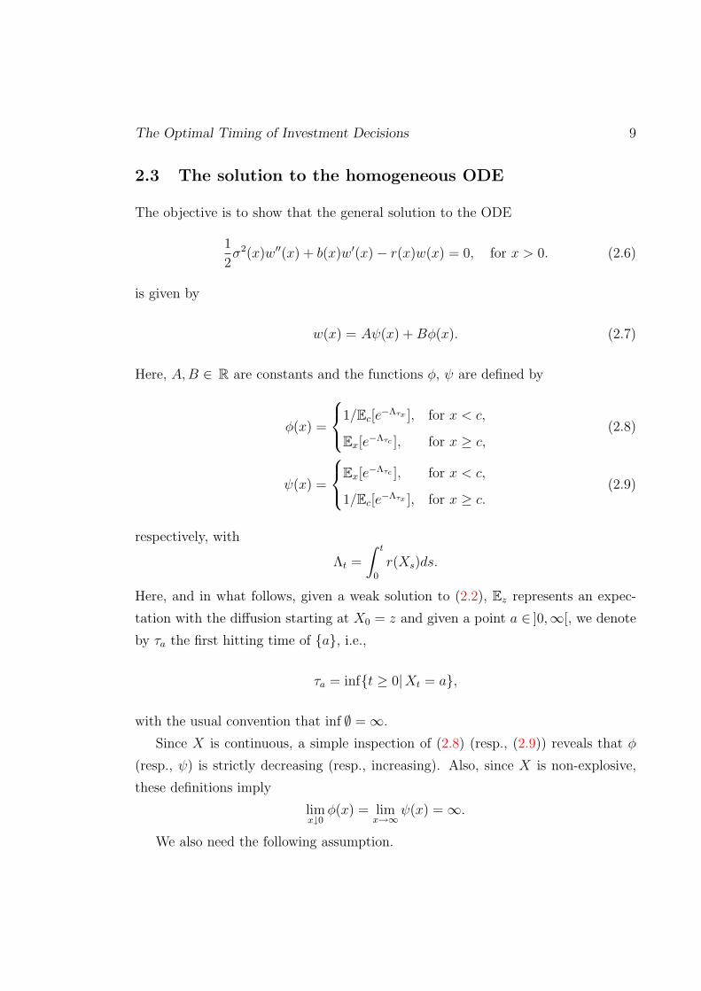
2.3 The solution to the homogeneous ODE
The objective is to show that the general solution to the ODE
1
2σ2(x)w′′(x) + b(x)w′(x)− r(x)w(x) = 0, for x > 0. (2.6)
is given by
w(x) = Aψ(x) +Bφ(x). (2.7)
Here, A,B ∈ R are constants and the functions φ, ψ are defined by
φ(x) =
1/Ec[e−Λτx ], for x < c,
Ex[e−Λτc ], for x ≥ c,
(2.8)
ψ(x) =
Ex[e−Λτc ], for x < c,
1/Ec[e−Λτx ], for x ≥ c.
(2.9)
respectively, with
Λt =
∫ t
0
r(Xs)ds.
Here, and in what follows, given a weak solution to (2.2), Ez represents an expec-
tation with the diffusion starting at X0 = z and given a point a ∈ ]0,∞[, we denote
by τa the first hitting time of a, i.e.,
τa = inft ≥ 0|Xt = a,
with the usual convention that inf ∅ = ∞.
Since X is continuous, a simple inspection of (2.8) (resp., (2.9)) reveals that φ
(resp., ψ) is strictly decreasing (resp., increasing). Also, since X is non-explosive,
these definitions imply
limx↓0
φ(x) = limx→∞
ψ(x) = ∞.
We also need the following assumption.

The Optimal Timing of Investment Decisions 10
Assumption 2.3.1 The function r :]0,∞[→ ]0,∞[ is locally bounded.
One purpose of the following result is to show that the definitions of φ, ψ in (2.8),
(2.9), respectively, do not depend, in a non-trivial way, on the choice of c ∈ ]0,∞[.
Lemma 2.3.1 Suppose that Assumptions 2.2.1–2.3.1 hold. Given any x, y ∈ ]0,∞[
the functions φ, ψ defined by (2.8), (2.9), respectively, satisfy
φ(y) = φ(x)Ey[e−Λτx ] and ψ(x) = ψ(y)Ex[e
−Λτy ], for all x < y. (2.10)
Moreover, the processes (e−Λtφ(Xt), t ≥ 0) and (e−Λtψ(Xt), t ≥ 0) are both local
martingales.
Proof. Given any points a, b, c ∈ ]0,∞[ such that a < b < c, we calculate
Ea[e−Λτc ] = Ea
[eΛτb Ea[e
−(Λτc−Λτb)|Fτb ]
]= Ea[e
−Λτb ]Eb[e−Λτc ],
where the second equality follows thanks to the strong Markov property of X. In
view of this result, given any x < z < y, the choice a = x, b = z and c = y yields
Ex[e−Λτy ] = Ex[e
−Λτz ]Ez[e−Λτy ],
which, combined with the definition of ψ, implies the second identity in (2.10). We
can verify the second identity in (2.10) when x < y < z or z < x < y as well as the
second identity in (2.10) by appealing to similar arguments.
Now, given any initial condition x and any sequence (xn) such that x < x1 and
limn→∞ xn = sup ]0,∞[, we observe that the second identity in (2.10) implies
ψ(Xt)1t≤τxn = ψ(xn)EXt [e−Λτxn ]1t≤τxn, for all t ≥ 0.
In view of this identity, we appeal to the strong Markov property of X, once again

The Optimal Timing of Investment Decisions 11
to calculate
Ex
[e−Λτxnψ(Xτxn
)∣∣Ft] = e−Λtψ(xn)Ex
[e−(Λτxn−Λt)
∣∣Ft]1t<τxn + e−Λτxnψ(xn)1τxn≤t
= e−Λtψ(Xt)1t<τxn + e−Λτxnψ(xn)1τxn≤t
= e−Λ(t∧τxn )ψ(Xt∧τxn).
However, this calculation and the tower property of conditional expectation implies
that, given any times s < t,
Ex
[e−Λt∧τxnψ(Xt∧τxn
)|Fs]
= Ex
[Ex
[e−Λt∧τxnψ(Xt∧τxn
)∣∣Ft] ∣∣Fs]
= e−Λs∧τxnψ(Xs∧τxn),
which proves that(e−Λtψ(Xt), t ≥ 0
)is a local-martingale. Proving that(
e−Λtφ(Xt), t ≥ 0)
is a local-martingale follows similar arguments. 2
We can now prove the following result.
Theorem 2.3.1 Suppose that Assumptions 2.2.1–2.3.1 hold. The general solution
to the ordinary differential equation (2.6) exists in the classical sense, namely there
exists a two dimensional space of functions that are C1 with absolutely continuous
first derivatives, and that satisfy (2.6) Lebesgue-a.e.. This solution is given by (2.7),
where A,B ∈ R are constants and the functions φ, ψ are given by (2.8), (2.9),
respectively. Moreover, φ is strictly decreasing, ψ is strictly increasing, and, if the
drift b ≡ 0, then both φ and ψ are strictly convex.
Proof. First, we recall that, given l < x < m,
Px(τl < τm) =pc(x)− pc(m)
pc(l)− pc(m)(2.11)
(e.g., see Karatzas and Shreve [KS91, Proposition 5.5.22] or Rogers and Williams
[RW94, Definition V.46.10]). Also in view of the second identity in (2.10), we can

The Optimal Timing of Investment Decisions 12
see that
ψ(x) < ψ(m)Ex
[1τm<τl
]+ ψ(m)Ex
[e−Λτm 1τl<τm
]= ψ(m)Px(τm < τl) + ψ(m)Ex
[Ex
[e−Λτm
∣∣Fτl] 1τl<τm].
Now, since X has the strong Markov property we can see that
Ex
[e−Λτm
∣∣Fτl]1τl<τm = e−Λτl Ex
[e−Λ(τm−τl) |Fτl
]1τl<τm
= e−Λτlψ(l)
ψ(m)1τl<τm,
with the last equality following thanks to (2.10). Combining these calculations we
can see that
ψ(x) < ψ(m)Px(τm < τl) + ψ(l)Ex
[e−Λτl 1τl<τm
]< ψ(m)Px(τm < τl) + ψ(l)Px(τl < τm). (2.12)
Now, let us assume that b ≡ 0, so that the diffusion X defined by (2.2) is in
natural scale, in which case pc(x) = x − c. Combining this fact with (2.11), it is
straightforward to verify that
x = lPx(τl < τm) +mPx(τm < τl).
However, this calculation and (2.12) imply that ψ is strictly convex. In this case,
we have also that
Px(τl < τm) =x−m
l −m. (2.13)
Under the assumption that b ≡ 0, which implies that ψ is strictly convex, we

The Optimal Timing of Investment Decisions 13
can use the Ito-Tanaka and the occupation times formulae to calculate
ψ(Xt)−∫ t
0
r(Xs)ψ(Xs) ds = ψ(x) +
∫]0,∞[
Lat1
σ2(a)
[1
2σ2(a)µ′′(da)− r(a)ψ(a) da
]+
∫ t
0
ψ′−(Xs)σ(Xs) dWs,
where ψ′− is the left-hand-side first derivative of ψ, µ′′(da) is the distributional second
derivative of ψ, and La is the local time process of X at level a. With regard to the
integration by parts formula, this implies
e−Λtψ(Xt) = ψ(x) +
∫ t
0
e−Λs d
∫]0,∞[
Las1
σ2(a)
[1
2σ2(a)µ′′(da)− r(a)ψ(a) da
]+
∫ t
0
e−Λsψ′−(Xs)σ(Xs) dWs.
Since (e−Λtψ(Xt), t ≥ 0) is a local-martingale (see Lemma 2.3.1), this identity
implies that the finite variation process Q defined by
Qt =
∫ t
0
e−Λsd
∫]0,∞[
Las1
σ2(a)
[1
2σ2(a)µ′′(da)− r(a)ψ(a) da
], for t ≥ 0,
is a local martingale. Since finite-variation local martingales are constant, it follows
that Q ≡ 0, which implies∫]0,∞[
Lat ν(da) = 0, for all t ≥ 0, (2.14)
where the measure ν is defined by
ν(da) =1
2µ′′(da)− r(a)ψ(a)
σ2(a)ψ′′(a). (2.15)
To proceed further, fix any points l < a < m, define
τl,m = inf t ≥ 0 |Xt /∈ ]l,m[ ,
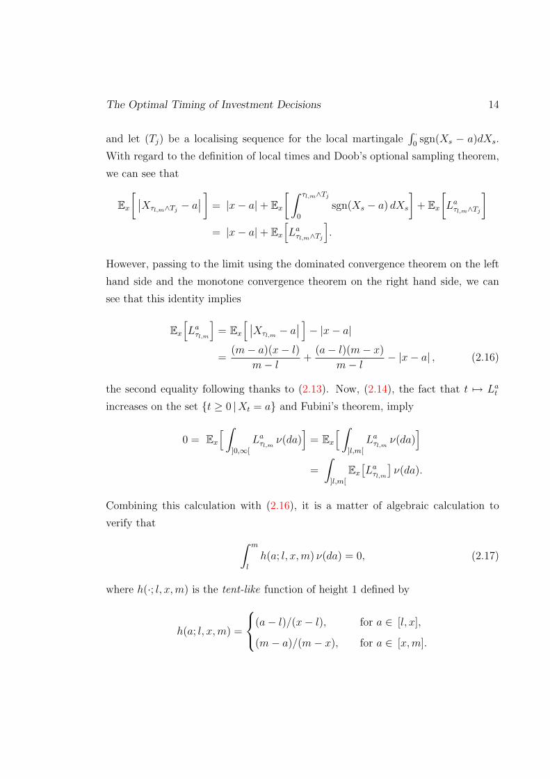
The Optimal Timing of Investment Decisions 14
and let (Tj) be a localising sequence for the local martingale∫ ·
0sgn(Xs − a)dXs.
With regard to the definition of local times and Doob’s optional sampling theorem,
we can see that
Ex
[ ∣∣Xτl,m∧Tj− a∣∣ ] = |x− a|+ Ex
[ ∫ τl,m∧Tj
0
sgn(Xs − a) dXs
]+ Ex
[Laτl,m∧Tj
]= |x− a|+ Ex
[Laτl,m∧Tj
].
However, passing to the limit using the dominated convergence theorem on the left
hand side and the monotone convergence theorem on the right hand side, we can
see that this identity implies
Ex
[Laτl,m
]= Ex
[ ∣∣Xτl,m − a∣∣ ]− |x− a|
=(m− a)(x− l)
m− l+
(a− l)(m− x)
m− l− |x− a| , (2.16)
the second equality following thanks to (2.13). Now, (2.14), the fact that t 7→ Lat
increases on the set t ≥ 0 |Xt = a and Fubini’s theorem, imply
0 = Ex
[ ∫]0,∞[
Laτl,m ν(da)]
= Ex
[ ∫]l,m[
Laτl,m ν(da)]
=
∫]l,m[
Ex
[Laτl,m
]ν(da).
Combining this calculation with (2.16), it is a matter of algebraic calculation to
verify that ∫ m
l
h(a; l, x,m) ν(da) = 0, (2.17)
where h(·; l, x,m) is the tent-like function of height 1 defined by
h(a; l, x,m) =
(a− l)/(x− l), for a ∈ [l, x],
(m− a)/(m− x), for a ∈ [x,m].

The Optimal Timing of Investment Decisions 15
Now, fix any points xl < xm in ]0,∞[ and let (lj) and (mj) be strictly decreasing
and strictly increasing, respectively, sequences such that
l1 <xl + xm
2< m1, lim
j→∞lj = xl and lim
j→∞mj = xm.
We can see that
1]xl,xm[(a) = limj→∞
Hj(a), for all a ∈ ]0,∞[,
where the increasing sequence of functions (Hj) is defined by
Hj(a) = h
(a;xl,
xl + xm2
, xm
)+xl + xm − 2ljxm − xl
h
(a;xl, lj,
xl + xm2
)+
2mj − (xl + xm)
xm − xlh
(a;xl + xm
2,mj, xm
), for a ∈ ]0,∞[ and j ≥ 1.
Using the monotone convergence theorem and (2.17), it follows that
ν(]xl, xm[) = limj→∞
∫ xm
xl
Hj(a) ν(da) = 0,
which proves that the signed measure ν assigns measure 0 to every open subset
of ]0,∞[. However, this observation and the definition of ν in (2.15) imply that
the total variation of ν is zero, and, therefore, µ′′(da) is an absolutely continuous
measure. It follows that there exists a function ψ′′ such that
µ′′(da) = ψ′′(a) da and1
2σ2(a)ψ′′(a) = r(a)ψ(a), Lebesgue-a.e..
However, the second identity here shows that ψ is a classical solution to (2.6).
Now, let us consider the general case where the drift b does not vanish. In this

The Optimal Timing of Investment Decisions 16
case, we use Ito’s formula to verify that, if X = pc(X), then
dXt = σ(Xt)dWt, X0 = pc(x),
where
σ(x) = p′c(p−1c (x)
)σ(p−1c (x)
), for x ∈ ]0,∞[.
Since X is a diffusion in natural scale, the associated function ψ defined as in (2.9)
is a classical solution of
1
2σ2(a)ψ′′(a)− r(a)ψ(a) = 0. (2.18)
Now, recalling that pc is twice differentiable in the classical sense, we can see that
if we define ψ(x) = ψ(pc(x)) then
ψ′(x) = ψ′(pc(x)
)p′c(x),
ψ′′(x) = ψ′′(pc(x)
)[p′c(x)
]2+ ψ′
(pc(x)
)p′′c (x).
However, combining these calculations with (2.18), we can see that ψ satisfies the
ODE (2.6).
To prove that ψ, namely the classical solution to (2.6), as constructed above,
identifies with ψ defined by (2.9), we apply Ito’s formula to e−Λ(τy∧T )ψ(Xτy∧T ), where
T > 0 is a constant, and we use arguments similar to the ones employed in the proof
of Theorem 3.3.1, to show that
Ex
[e−Λτy∧T ψ(Xτy∧T )
]= ψ(x), for all x < y.
Since ψ > 0 is increasing, the monotone and the dominated convergence theorems
imply
limT→∞
Ex
[e−Λτy∧T ψ(Xτy∧T )
]= ψ(y)Ex
[e−Λτy
], for all x < y.
However, these calculations, show that ψ satisfies the second identity in (2.10) and

The Optimal Timing of Investment Decisions 17
therefore identifies with ψ defined by (2.9). Proving all of the associated claims for
φ follows similar reasoning. 2
Remark 2.3.1 Although we have chosen to undertake this analysis for a positive
diffusion, similar results can be obtained for a regular Ito diffusion with values in
any interval I where I ⊆ R.
Using the fact that φ and ψ satisfy the ODE (2.6), it is a straightforward exercise
to verify that the scale function, pc, defined by (2.3) satisfies
p′c(x) =φ(x)ψ′(x)− φ′(x)ψ(x)
W(c), for all x > 0, (2.19)
where W is the Wronskian of φ and ψ, defined by
W(x) = φ(x)ψ′(x)− φ′(x)ψ(x)
and W(x) > 0 for all x > 0.
2.4 Study of a non-homogeneous ordinary differential equa-
tion
We now study the non-homogeneous ODE (2.1),
1
2σ2(x)w′′(x) + b(x)w′(x)− r(x)w(x) + h(x) = 0, x ∈ ]0,∞[.
We need to impose the following assumptions, which are stronger than Assump-
tion 2.2.1 and Assumption 2.3.1, respectively.
Assumption 2.2.1′ The conditions of Assumption 2.2.1 hold true, and
the function σ is locally bounded.

The Optimal Timing of Investment Decisions 18
Assumption 2.3.1′ The conditions of Assumption 2.3.1 hold true, and there exists
a constant r0 such that
0 < r0 ≤ r(x) <∞, for all x > 0. (2.20)
We can now prove the following propositions.
Proposition 2.4.1 Suppose that Assumption 2.2.1′, Assumption 2.2.2 and Assump-
tion 2.3.1′ hold. The following statements are equivalent:
(I) Given any initial condition x > 0 and any weak solution Sx to (2.2),
Ex
[∫ ∞
0
e−Λt|h(Xt)| dt]<∞.
(II) There exists an initial condition y > 0 and a weak solution Sy to (2.2) such
that
Ey
[∫ ∞
0
e−Λt|h(Xt)| dt]<∞.
(III) Given any x > 0,∫ x
0
|h(s)|ψ(x)m(ds) <∞ and
∫ ∞
x
|h(s)|φ(x)m(ds) <∞.
(IV) There exists y > 0 such that∫ y
0
|h(s)|ψ(x)m(ds) <∞ and
∫ ∞
y
|h(s)|φ(x)m(ds) <∞.
If these conditions hold, then the function
Rh(x) =φ(x)
W(c)
∫ x
0
h(s)ψ(s)m(ds) +ψ(x)
W(c)
∫ ∞
x
h(s)φ(s)m(ds), x ∈ ]0,∞[,
(2.21)

The Optimal Timing of Investment Decisions 19
is well-defined, is twice differentiable in the classical sense and satisfies the ODE
(2.1), Lebesgue-a.e.. In addition, Rh admits the expression
Rh(x) = Ex
[∫ ∞
0
e−Λsh(Xs) ds
], for all x > 0. (2.22)
Proof. Suppose that (IV) is true and let y be such that
C1 :=
∫ y
0
|h(s)|ψ(s)m(ds) <∞ and C2 :=
∫ ∞
y
|h(s)|φ(s)m(ds) <∞.
and so∫ x
0
|h(s)|ψ(s)m(ds),
∫ y
x
|h(s)|ψ(s)m(ds) ≤ C1, for all x ∈ ]0, y[, (2.23)∫ x
y
|h(s)|φ(s)m(ds),
∫ ∞
x
|h(s)|φ(s)m(ds) ≤ C2, for all x ∈ ]y,∞[. (2.24)
Combining these inequalities with the fact that ψ is increasing and φ is decreasing,
we can see that∫ ∞
x
|h(s)|φ(s)m(ds) =
∫ y
x
|h(s)|φ(s)m(ds) +
∫ ∞
y
|h(s)|φ(s)m(ds)
≤ φ(x)
ψ(x)
∫ y
x
|h(s)|ψ(s)m(ds) + C2
≤ φ(x)
ψ(x)C1 + C2
< ∞ (2.25)

The Optimal Timing of Investment Decisions 20
and ∫ x
0
|h(s)|ψ(s)m(ds) =
∫ y
0
|h(s)|ψ(s)m(ds) +
∫ x
y
|h(s)|ψ(s)m(ds)
≤ C1 +ψ(x)
φ(x)
∫ x
y
|h(s)|φ(s)m(ds)
≤ C1 +ψ(x)
φ(x)C2
< ∞. (2.26)
However, (2.23)–(2.26) imply that (III) holds. The reverse implication is obvious.
To proceed further, assume that h = h+B where h+
B is a positive and bounded mea-
surable function. In this case, it is straightforward to verify that (I) and (II) are both
satisfied. Since φ and ψ are continuous functions satisfying limx→∞ φ(x), limx↓0 ψ(x) <
∞ and m is a locally finite measure, the function Rh+B1[1/k,k]
: ]0,∞[→ R+ given by
(2.21), or, equivalently, by
Rh+B1[1/k,k]
(x) =φ(x)
W(c)1[1/k,k](x)
∫ x
1/k
h+B(s)ψ(s)m(ds)
+ψ(x)
W(c)1[1/k,k](x)
∫ k
x
h+B(s)φ(s)m(ds), (2.27)
is well-defined and bounded for all k > 1. In light of the calculations
R′h+B1[1/k,k]
(x) =φ′(x)
W(c)
∫ x
0
h+B(s)1[1/k,k](s)ψ(s)m(ds)
+ψ′(x)
W(c)
∫ ∞
x
h+B(s)1[1/k,k](s)φ(s)m(ds),
R′′h+B1[1/k,k]
(x) =φ′′(x)
W(c)
∫ x
0
h+B(s)1[1/k,k](s)ψ(s)m(ds)
+ψ′′(x)
W(c)
∫ ∞
x
h+B(s)1[1/k,k](s)φ(s)m(ds)
− 2h+B(x)
σ2(x)1[1/k,k](x)
we can see that Rh+B1[1/k,k]
is twice differentiable in the classical sense, because this

The Optimal Timing of Investment Decisions 21
is true for the functions ψ and φ, and satisfies the ODE
1
2σ2(x)w′′(x) + b(x)w′(x)− r(x)w(x) + h+
B(x)1[1/k,k](x) = 0, (2.28)
Lebesgue-a.e. in ]0,∞[.
Now, fix any k > 1, any initial condition x > 0, any weak solution Sx to (2.2)
and define the sequence of (Ft)-stopping times (τl) by
τl = inf t ≥ 0 | Xt /∈ [1/l, l] ,
Using Ito’s formula and the fact that Rh+B1[1/k,k]
satisfies (2.28), we calculate
e−Λτl∧TRh+B1[1/k,k]
(Xτl∧T ) +
∫ τl∧T
0
e−Λsh+B(Xs)1[1/k,k](Xs) ds
= Rh+B1[1/k,k]
(x) +M(l)t , (2.29)
where M (l) is defined by
M(l)t =
∫ τl∧t
0
e−Λsσ(Xs)R′h+B1[1/k,k]
(Xs) dWs.
Combining the fact that R′h+B1[1/k,k]
is locally bounded, because Rh+B1[1/k,k]
is continu-
ous, with the the fact that σ is locally bounded from Assumption 2.2.1′, we can see
that the quadratic variation of the local martingale M(l)t satisfies
Ex
[〈M (l)〉∞
]=
∫ ∞
0
Ex
[1s≤τl
(e−Λsσ(Xs)R
′h+B1[1/k,k]
(Xs))2]ds
≤ supy∈[1/l,l]
[σ(y)R′
h+B1[1/k,k]
(y)]2 ∫ ∞
0
Ex
[e−2Λs
]ds
≤ 1
2r0sup
y∈[1/l,l]
[σ(y)R′
h+B1[1/k,k]
(y)]2
<∞,
the second inequality following as a consequence of (2.20) in Assumption 2.3.1′. This

The Optimal Timing of Investment Decisions 22
proves that M (l) is a martingale bounded in L2, so, Ex
[M
(l)t
]= 0, for all t ≥ 0.
This observation and (2.29) imply
Ex
[e−Λτl∧TRh+
B1[1/k,k](Xτl∧T ) +
∫ τl∧T
0
e−Λsh+B(Xs)1[1/k,k] ds
]= Rh+
B1[1/k,k](x).
(2.30)
Since Rh+B1[1/k,k]
is bounded, the dominated convergence theorem implies
limT→∞
liml→∞
Ex
[e−Λτl∧TRh+
B1[1/k,k](Xτl∧T )
]= 0,
while the monotone convergence theorem yields
limT→∞
liml→∞
Ex
[∫ τl∧T
0
e−Λsh+B(Xs)1[1/k,k](Xs) ds
]= Ex
[∫ ∞
0
e−Λsh+B(Xs)1[1/k,k](Xs) ds
].
These limits and (2.30) imply
Ex
[∫ ∞
0
e−Λsh+B(Xs)1[1/k,k](Xs) ds
]= Rh+
B1[1/k,k](x).
Recalling the definition of Rh+B1[1/k,k]
as in (2.27), we can pass to the limit k → ∞in this identity to obtain
Rh+B(x) = Ex
[∫ ∞
0
e−Λsh+B(Xs) ds
]. (2.31)
Note that, since, h+B plainly satisfies conditions (I) and (II), this identity also implies
that h+B satisfies conditions (III) and (IV).
Now assume that h = h+, where h+ is a positive measurable function. Using
(2.31) with h+B = h+∧n, for n ≥ 1, and applying the monotone convergence theorem,
we can see that, given any initial condition x > 0 and any weak solution Sx to (2.2),
Ex
[∫ ∞
0
e−Λsh+(Xs) ds
]= Rh+(x), (2.32)
The Optimal Timing of Investment Decisions 23
where both sides may be equal to infinity. However, with reference to the definition
of Rh+ , this proves that (I) and (III) are equivalent and that (II) and (IV) imply each
other. Recalling the equivalence of (III) and (IV) that we proved above, it follows
that statements (I)–(IV) are all equivalent. Furthermore, given any h satisfying
(I)–(IV), we can immediately see that (2.32) implies (2.22) once we consider the
decomposition h = h+ − h− of h to its positive and its negative parts h+ and h−,
respectively. 2
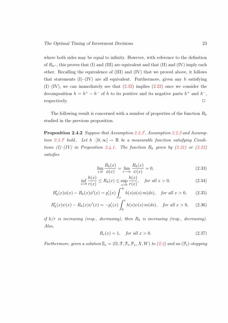
The following result is concerned with a number of properties of the function Rh
studied in the previous proposition.
Proposition 2.4.2 Suppose that Assumption 2.2.1′, Assumption 2.2.2 and Assump-
tion 2.3.1′ hold.. Let h : ]0,∞[→ R be a measurable function satisfying Condi-
tions (I)–(IV) in Proposition 2.4.1. The function Rh given by (2.21) or (2.22)
satisfies
limx↓0
Rh(x)
φ(x)= lim
x→∞
Rh(x)
ψ(x)= 0, (2.33)
infx>0
h(x)
r(x)≤ Rh(x) ≤ sup
x>0
h(x)
r(x), for all x > 0, (2.34)
R′h(x)φ(x)−Rh(x)φ
′(x) = p′c(x)
∫ ∞
x
h(s)φ(s)m(ds), for all x > 0, (2.35)
R′h(x)ψ(x)−Rh(x)ψ
′(x) = −p′c(x)∫ x
0
h(s)ψ(s)m(ds), for all x > 0, (2.36)
if h/r is increasing (resp., decreasing), then Rh is increasing (resp., decreasing).
Also,
Rr(x) = 1, for all x > 0. (2.37)
Furthermore, given a solution Sx = (Ω,F,Ft,Px, X,W ) to (2.2) and an (Ft)-stopping

The Optimal Timing of Investment Decisions 24
time τ ,
Ex
[e−ΛτRh(Xτ )1τ<∞
]= Rh(x)− Ex
[∫ τ
0
e−Λth(Xt) dt
], (2.38)
Ex
[e−ΛτRh(Xτ )1τ<∞
]= Ex
[∫ ∞
τ
e−Λth(Xt) dt
], (2.39)
while, if (τn) is a sequence of stopping times such that limn→∞ τn = ∞, Px-a.s., then
limn→∞
Ex
[e−Λτn |Rh(Xτn)|1τn<∞
]= 0. (2.40)
Proof. Fix a solution Sx = (Ω,F,Ft,Px, X,W ) to (2.2) and let τ be an (Ft)-stopping
time. Using the definition of Λ and the strong Markov property of X, we can see
that (2.22) implies
Rh(x) = Ex
[∫ τ
0
e−Λth(Xt) dt+ e−Λτ Ex
[∫ ∞
τ
e−(Λs−Λτ )h(Xs) ds | Fτ]1τ<∞
]= Ex
[∫ τ
0
e−Λth(Xt) dt+ e−Λτ EXτ
[∫ ∞
0
e−Λsh(Xs) ds
]1τ<∞
]= Ex
[∫ τ
0
e−Λth(Xt) dt+ e−ΛτRh(Xτ )1τ<∞
],
which establishes (2.38). Also, this expression and (2.22) imply immediately (2.39),
while (2.40) follows from the observation that |Rh| ≤ R|h| (note that h satisfies
conditions (I)–(IV) of Proposition 2.4.1 if and only in |h| does), (2.39) and the
dominated convergence theorem.
Now, let c > 0 be the point that we used in (2.3) and (2.4) to define the
scale function and the speed measure of the diffusion X. Given a solution Sc =
(Ω,F,Ft,Pc, X,W ) to (2.2) and any x > 0, we denote by τx the first hitting time of
x, and we note that limx↓0 τx = limx→∞ τx = ∞, Pc-a.s., because the diffusion X
is non-explosive by Assumption 2.2.2. In view of this observation and the fact that
r(x) ≥ r0 > 0, for all x > 0, by Assumption 2.3.1′, we have that (2.40) implies
limx↓0
Ec
[e−Λτx
]Rh(x) = lim
x→∞Ec
[e−Λτx
]Rh(x) = 0.

The Optimal Timing of Investment Decisions 25
However, these limits and the definitions (2.8) and (2.9) of the functions φ and ψ
imply (2.33). Also, a simple inspection of the ODE (2.1) reveals that if we set
h = r then Rr satisfies (2.37), noting that Rr is well-defined thanks to (2.20) in
Assumption 2.3.1′. We can verify (2.35) and (2.36) by a straightforward calculation
using the definition (2.21) of Rh and (2.19).
To proceed further, let us assume that h/r is increasing, let us fix any x > 0,
and let us define Cx = h(x)/r(x). In view of (2.38), the monotonicity of h/r, and
the definition (2.9) of ψ we calculate
Rh(·)−Cxr(·)(x− ε) = Ex−ε
[∫ τx
0
e−Λt [h(Xt)− Cxr(Xt)] dt
]+Rh(·)−Cxr(·)(x)Ex−ε
[e−Λτx
]≤ Rh(·)−Cxr(·)(x)
ψ(x− ε)
ψ(x), for all ε > 0, (2.41)
which shows that
Rh(·)−Cxr(·)(x)−Rh(·)−Cxr(·)(x− ε)
ε≥Rh(·)−Cxr(·)(x)
ψ(x)
ψ(x)− ψ(x− ε)
ε, for all ε > 0.
Recalling that Rh(·)−Cxr(·) is C1, we can pass to the limit ε ↓ 0 in this inequality to
obtain
R′h(·)−Cxr(·)(x) ≥ Rh(·)−Cxr(·)(x)
ψ′(x)
ψ(x). (2.42)
Making a calculation similar to the one in (2.41) using the definition (2.8) of φ this
time, we can see that
Rh(·)−Cxr(·)(x+ ε) ≥ Rh(·)−Cxr(·)(x)φ(x+ ε)
φ(x), for all ε > 0.
Rearranging terms and passing to the limit ε ↓ 0, we can see that this inequality
implies
R′h(·)−Cxr(·)(x) ≥ Rh(·)−Cxr(·)(x)
φ′(x)
φ(x). (2.43)

The Optimal Timing of Investment Decisions 26
Recalling that the strictly positive function ψ is strictly increasing and that the
strictly positive function φ is strictly decreasing, we can see that (2.42) implies
R′h(·)−Cxr(·)(x) ≥ 0 if Rh(·)−Cxr(·)(x) ≥ 0, while, (2.43) implies R′
h(·)−Cxr(·)(x) ≥ 0
if Rh(·)−Cxr(·)(x) ≤ 0. Now, combining the inequality Rh(·)−Cxr(·)(x) ≥ 0 with the
identities
R′h(·)−Cxr(·)(x) =
φ′(x)
W(c)
∫ x
0
[h(s)− Cxr(s)]ψ(s)m(ds)
+ψ′(x)
W(c)
∫ ∞
x
[h(s)− Cxr(s)]φ(s)m(ds)
= R′h(x)− CxR
′r(x)
= R′h(x)
that follow from the definition (2.21) of Rh and (2.37), we can see that R′h(x) ≥ 0.
However, since the point x > 0 has been arbitrary, this analysis establishes the claim
that, if h/r is increasing, then Rh is increasing. Proving the claim corresponding to
the case when h/r is decreasing follows similar symmetric arguments.
Finally, to show (2.34), let us assume that h := infx>0 h(x)/r(x) > −∞. In this
case, we can use (2.37) and the representation (2.22) to calculate
Rh(x)− infx>0
h(x)
r(x)= Rh(x)−Rhr(·)(x)
= Ex
[∫ ∞
0
e−Λt
[h(Xt)− inf
x>0
h(x)
r(x)r(Xt)
]dt
]≥ 0,
which establishes the lower bound in (2.34). The upper bound in (2.34) can be
established in exactly the same way, and the proof is complete. 2

The Optimal Timing of Investment Decisions 27
The following lemma gives result useful for practical applications.
Lemma 2.4.1 Suppose that Assumption 2.2.1′, Assumption 2.2.2 and Assump-
tion 2.3.1′ hold. Let h : ]0,∞[→ R be a measurable function satisfying Condi-
tions (I)–(IV) in Proposition 2.4.1. If, in addition, h/r is increasing, then if 0 is a
natural boundary (not an entrance boundary) then
limx↓0
Rh(x) = limx↓0
h(x)
r(x), (2.44)
and if ∞ is a natural boundary then
limx→∞
Rh(x) = limx→∞
h(x)
r(x). (2.45)
Proof We have
Rh(x) ≤ supx>0
h(x)
r(x)Ex
[∫ ∞
0
d(e−Λt)
)]= sup
x>0
h(x)
r(x)
and
Rh(x) ≥ infx>0
h(x)
r(x)Ex
[∫ ∞
0
d(e−Λt)
)]= inf
x>0
h(x)
r(x).
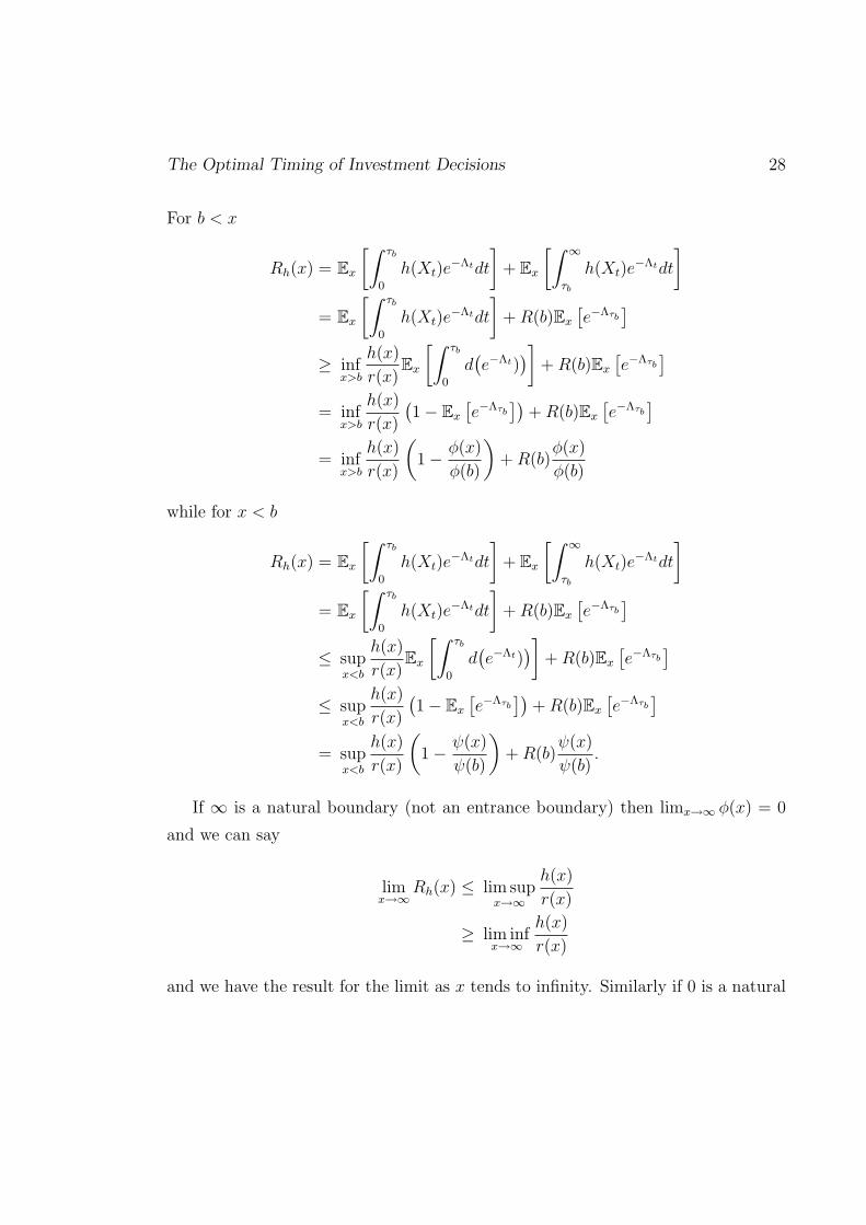
The Optimal Timing of Investment Decisions 28
For b < x
Rh(x) = Ex
[∫ τb
0
h(Xt)e−Λtdt
]+ Ex
[∫ ∞
τb
h(Xt)e−Λtdt
]= Ex
[∫ τb
0
h(Xt)e−Λtdt
]+R(b)Ex
[e−Λτb
]≥ inf
x>b
h(x)
r(x)Ex
[∫ τb
0
d(e−Λt)
)]+R(b)Ex
[e−Λτb
]= inf
x>b
h(x)
r(x)
(1− Ex
[e−Λτb
])+R(b)Ex
[e−Λτb
]= inf
x>b
h(x)
r(x)
(1− φ(x)
φ(b)
)+R(b)
φ(x)
φ(b)
while for x < b
Rh(x) = Ex
[∫ τb
0
h(Xt)e−Λtdt
]+ Ex
[∫ ∞
τb
h(Xt)e−Λtdt
]= Ex
[∫ τb
0
h(Xt)e−Λtdt
]+R(b)Ex
[e−Λτb
]≤ sup
x<b
h(x)
r(x)Ex
[∫ τb
0
d(e−Λt)
)]+R(b)Ex
[e−Λτb
]≤ sup
x<b
h(x)
r(x)
(1− Ex
[e−Λτb
])+R(b)Ex
[e−Λτb
]= sup
x<b
h(x)
r(x)
(1− ψ(x)
ψ(b)
)+R(b)
ψ(x)
ψ(b).
If ∞ is a natural boundary (not an entrance boundary) then limx→∞ φ(x) = 0
and we can say
limx→∞
Rh(x) ≤ lim supx→∞
h(x)
r(x)
≥ lim infx→∞
h(x)
r(x)
and we have the result for the limit as x tends to infinity. Similarly if 0 is a natural

The Optimal Timing of Investment Decisions 29
boundary then limx→∞ ψ(x) = 0 and we can say
limx↓0
Rh(x) ≤ lim supx↓0
h(x)
r(x)
≥ lim infx↓0
h(x)
r(x)
and we have the result for the limit as x tends to zero. 2
Remark 2.4.1 In the cases where we do not have a natural boundary point, Rh
does not converge to a value determined in a straightforward way by h and r in
the limit. To see this, consider the case of the so-called square root mean reverting
process, defined by
dXt = κ(θ −Xt) dt+ σ√Xt dWt, X0 = x > 0,
where κ, θ and σ are positive constants satisfying κθ− 12σ2 > 0. Note that this dif-
fusion has an entrance boundary point at zero. It is a standard exercise to calculate
that
Ex[Xt] = θ + (x− θ)e−κt,
Ex
[X2t
]=
(σ2θ
2κ+ θ2
)+ e−κt
(2θ(x− θ)− 2
σ2θ
2κ+σ2x
κ
)+ e−2κt
(σ2θ
2κ− σ2x
κ+ (x− θ)2
).
Now, let us consider the following three cases for the payoff function, h:
h1(x) = 0, h2(x) = x and h3(x) = x2.
and assume that r is a constant. In all these cases limx↓0 h(x)/r(x) = 0. However,

The Optimal Timing of Investment Decisions 30
we can see that
limx↓0
Rh1(x) = 0,
limx↓0
Rh2(x) =θκ
r(r + κ)> 0,
limx↓0
Rh3(x) =
(σ2θ
2κ+ θ2
)[2κ2
r(r + κ)(r + 2κ)
]> 0.

3. A DISCRETIONARY STOPPING
PROBLEM
3.1 Introduction
In this chapter we address a discretionary stopping problem as a prelude to address-
ing our investment problems. We solve this stopping problem general conditions on
the underlying diffusion, the payoff and the discounting. Also, we consider several
special cases. Although all of the special cases of interest that we are aware of are
associated with stochastic differential equations that have unique strong solutions,
we adopt a weak formulation. Working within this more general framework, which
involves no additional technicalities, has been motivated by the extra degrees of free-
dom that it offers relative to modelling and has a view to applications in stochastic
control beyond optimal stopping.
Section 3.2 is concerned with a rigorous formulation of the stopping problem that
we solve. In this section, we consider the case of the perpetual American call option
which highlights an issue related to waiting forever, which is mentioned in the intro-
duction in relation to McDonald and Siegel [MS86], namely that the problem data
may not conform to standard economic theory. Combining the observations from
this special case with the results of Section 2.4 we develop Assumption 3.2.1 that is
sufficient for our problem to conform with applications in finance and economics.
In Section 3.3 we solve the discretionary stopping problem. With reference to
the motivation of the thesis, we are particularly interested in identifying the nature
of the stopping boundary given the problem data and in solving the discretionary
stopping problem we distinguish cases based on the nature of the stopping boundary.
31

The Optimal Timing of Investment Decisions 32
In Section 3.4, we address a number of special cases of interest. These cases
involve a number of choices for the underlying state process X that have been
considered in the literature, while the payoff functions identify with standard utility
functions with the discount rate being assumed to be constant. In particular we
consider the cases that arise when X is a geometric Brownian motion; a square-
root mean-reverting process as in the Cox-Ingersoll-Ross interest rate model; and a
geometric Ornstein-Uhlenbeck process, which has been proposed by Cortazar and
Schwartz as a model for a commodity’s price and has been used in population
modelling.
3.2 Problem formulation and assumptions
We start by defining a stopping strategy.
Definition 3.2.1 Given an initial condition x > 0, a stopping strategy is any pair
(Sx, τ) such that Sx = (Ω,F,Ft,Px, X,W ) is a weak solution to (2.2) and τ is an
(Ft)-stopping-time. We denote by Sx the set of all such stopping strategies.
The objective is to maximise the performance criterion
J(Sx, τ) = Ex
[e−Λτ g(Xτ )1τ<∞
],
where Λt =∫ t
0r(Xs) ds and g : ] 0,∞[→ R and r : ]0,∞[→ ]0,∞[ are given deter-
ministic functions, over all stopping strategies (Sx, τ) ∈ Sx. Accordingly we define
the value function v by
v(x) = sup(Sx,τ)∈Sx
J(Sx, τ), for x > 0.
Now, with a view to developing an understanding of the problem under con-
sideration, we consider the case of a perpetual American call option written on an
underlying asset, the stochastic dynamics of which are modelled by a geometric
Brownian motion.

The Optimal Timing of Investment Decisions 33
Lemma 3.2.1 Suppose that X is a geometric Brownian motion, so that b(x) = bx
and σ(x) = σx, for some constants b and σ, and r(x) ≡ r > 0, for some constant
r. Suppose also that the payoff function is given by g(x) = x−K, where K ≥ 0 is a
constant. If b > r (resp., b < r), then the process (e−rtXt, t ≥ 0) is a submartingale
(resp., supermartingale) and v(x) = ∞ (resp., if K = 0, then v(x) = x).
Proof. Given any initial condition x > 0,
e−rtXt = xe(b−r)te−12σ2t+σWt , for t ≥ 0.
Combining this observation with the fact that the process (e−12σ2t+σWt , t ≥ 0) is a
martingale, we can see that all of the claims made are true. 2
In the context of this lemma, we can see that (Sx, 0) is an optimal strategy if
K = 0 and b < r. Given any K ≥ 0, if b − r > 12σ2, then the stopping strategy
(S∗x, τ ∗), where S∗x is a weak solution to (2.2) and
τ ∗ = inft ≥ 0| Wt = −a,
where a > 0 is any constant, provides an optimal strategy. Indeed, since τ ∗ < ∞,
Px-a.s., and Ex [τ ∗] = ∞, this claim follows from the calculation
Ex[e−rτ∗(Xτ∗ −K)] ≥ xe−aσEx
[e(b−r−
12σ2)τ∗
]−K
> xe−aσ[1 +
(b− r − 1
2σ2
)Ex[τ
∗]
]−K
= ∞.
When b > r and b − r < 12σ2, we have not been able to find an optimal stopping
strategy. As a matter of fact, we have been tempted to conjecture that there is no
optimal stopping strategy in this case.

The Optimal Timing of Investment Decisions 34
We note that, when b > r, which is associated with v ≡ ∞, and when b = r,
which is a case that we have not associated with a conclusion,
limt→∞
Ex
[e−Λtg(Xt)
]≡ lim
t→∞Ex
[e−rtXt
]> 0,
for all initial conditions x > 0. In this case, the problem data does not satisfy the
so-called transversality condition
limt→∞
Ex
[e−Λtg(Xt)
]≡ lim
t→∞Ex
[e−rtXt
]= 0.
Such a condition has a natural economic interpretation because it reflects the idea
that one should expect that the present value of any asset should be equal to zero
at the end of time, given that nobody can benefit by holding the asset after the
end of time. We expect that problems in finance and economics should satisfy this
condition.
Based on this observation and the results in Section 2.4, we impose the following
assumption in order to be able to carry out our analysis of the problem.
Assumption 3.2.1 The function g : ]0,∞[→ R is C1 with an absolutely continuous
first derivative. In addition, given any weak solution, Sx to (2.2) the function g
satisfies
Ex
[∫ ∞
0
e−Λt∣∣Lg(Xt)
∣∣dt] <∞, for all x > 0, (3.1)
where
Lg(x) :=1
2σ2(x)g′′(x) + b(x)g′(x)− r(x)g(x).
Remark 3.2.1 If we define the measurable function h as
h(x) = −Lg(x), for x > 0, (3.2)

The Optimal Timing of Investment Decisions 35
then, the function g satisfies the non-homogeneous ODE
1
2σ2(x)g′′(x) + b(x)g′(x)− r(x)g(x) + h(x) = 0, x ∈ ]0,∞[.
Therefore, by identifying Rh with g and by Propositions 2.4.1 and 2.4.2 in Sec-
tion 2.4, the following statements are true.
a. Given any weak solution, Sx to (2.2) and any (Ft)-stopping time, τ , the function
g satisfies
Ex
[e−Λτ g(Xτ )1τ<∞
]<∞, for all x > 0. (3.3)
In addition, Dynkin’s formula holds,
Ex
[e−Λτ g(Xτ )1τ<∞
]= g(x) + Ex
[(∫ τ
0
e−ΛtLg(Xt)dt
)1τ<∞
], for all x > 0.
(3.4)
b. The function g satisfies the following transversality condition. Given any weak
solution, Sx, to (2.2), if (τn) is a sequence of stopping times such that limn→∞ τn =
∞, Px-a.s., then
limn→∞
Ex
[e−Λτn |g(Xτn)|1τn<∞
]= 0. (3.5)
c. With reference to the functions φ and ψ, defined by (2.8) and (2.9), respectively,
and the scale function pc defined by (2.3), the function g satisfies the following
identities
limx↓0
g(x)
φ(x)= lim
x→∞
g(x)
ψ(x)= 0, (3.6)
g′(x)φ(x)− g(x)φ′(x) = −p′c(x)∫ ∞
x
Lg(s)φ(s)m(ds), for all x > 0, (3.7)
g′(x)ψ(x)− g(x)ψ′(x) = p′c(x)
∫ x
0
Lg(s)ψ(s)m(ds), for all x > 0. (3.8)

The Optimal Timing of Investment Decisions 36
Remark 3.2.2 In relation to the case of a perpetual American option, studied
above, we observe that
Ex
[∫ ∞
0
e−Λs |Lg(Xs)| ds]
= |(b− r)|∫ ∞
0
e(b−r)sds+K
and so the conditions laid out in Assumption 3.2.1 are not satisfied if b ≥ r, which
reflects some of the comments made earlier.
3.3 The solution to the discretionary stopping problem
In solving our stopping problem we shall employ the tools of dynamic programming
and break our overall problem into a series of sub-problems. We do this by consid-
ering, without loss of generality, our options at time zero, which are either to wait
or stop. Consider the case when we wait for a time ∆t and then continue optimally,
we expect that the value function v should satisfy the following inequality
v(x) ≥ Ex
[e−Λ∆T v(X∆T )
].
Using Ito’s formula, dividing by ∆t and taking the limit ∆t ↓ 0 yields
1
2σ2(x)v′′(x) + b(x)v′(x)− r(x)v(x) ≤ 0.
Alternatively, we can stop, and so we expect that
v(x) ≥ g(x).
We therefore expect that the value function v identifies with a solution w to the
Hamilton-Jacobi-Bellman (HJB) equation
max
1
2σ2(x)w′′(x) + b(x)w′(x)− r(x)w(x), g(x)− w(x)
= 0, x > 0. (3.9)
The Optimal Timing of Investment Decisions 37
To develop our intuition of the problem in hand further, consider the case where the
payoff is increasing. In this case we expect that there is a single boundary point,
x∗, separating the continuation and stopping regions and we postulate that it is
optimal to wait for as long as the state process X assumes values less than x∗ and
stop as soon as X hits the set [x∗,∞[. With reference to the heuristic arguments
given above, we therefore look for a solution w to (3.9) that satisfies
1
2σ2(x)w′′(x) + b(x)w′(x)− r(x)w(x) = 0, for x < x∗, (3.10)
g(x)− w(x) = 0, for x ≥ x∗. (3.11)
Such a solution is given by
w(x) =
Aφ(x) +Bψ(x), if x < x∗,
g(x), if x ≥ x∗,
where φ (resp., ψ) is the strictly decreasing (resp., increasing) function given by
(2.8) (resp., (2.9)). In addition, we expect that the value function is positive and
bounded near zero and so we must have A = 0. To specify the parameter B and
x∗, we appeal to the so-called “smooth-pasting” condition of optimal stopping that
requires the value function to be C1, in particular, at the free boundary point x∗.
This requirement yields the system of equations
Bψ(x∗) = g(x∗) and Bψ′(x∗) = g′(x∗),
which is equivalent to
B =g(x∗)
ψ(x∗)=g′(x∗)
ψ′(x∗)and q(x∗) = 0,
where q is defined by
q(x) = g(x)ψ′(x)− g′(x)ψ(x), x > 0,

The Optimal Timing of Investment Decisions 38
and we note that q(x∗) = 0 corresponds to a turning point of g/ψ, since ψ(x) > 0
for all x > 0.
To develop an intuition as to how g/ψ affects the stopping problem, consider a
different approach to solving the problem. Instead of looking for the stopping time
look for the stopping boundary, for example define the value function as
v(x) = supb
Ex
[e−Λτbg(b)
]= sup
bEx
[e−Λτb
]g(b)
Now, starting in the “continuation” region, so x < x∗ since g is increasing, we have
Ex[e−Λτb ] = ψ(x)/ψ(b)
and
v(x) = supb
(g(b)
ψ(b)
)ψ(x).
This approach is adopted in Beibel and Lerche [BL00], and provides a clear expla-
nation of why maxima of g/ψ or g/φ are of interest. Unfortunately, this approach
is of limited value when x > x∗.
With these comments in mind, we now provide the following verification theorem,
as a prelude to our main results. Note that the theorems in this section all rely on
Assumptions 2.2.1′, 2.2.2, 2.3.1′, 3.2.1, which are, respectively, that the SDE has
a weak solution, it is non-explosive, discounting is strictly positive and the payoffs
satisfy the transversality conditions.
Theorem 3.3.1 Suppose that Assumptions 2.2.1′, 2.2.2, 2.3.1′ and 3.2.1 hold. In
addition, suppose that the HJB equation (3.9) has a solution w and w ∈ C1(]0,∞[)∩C2(]0,∞[ \S), where S is a set of a finite number of points, then the value function
v defined in Section 3.2 identifies with w.
The Optimal Timing of Investment Decisions 39
Proof: Fix any initial condition x > 0 and any weak solution Sx to (2.2) and define
Mt =
∫ t
0
e−Λsσ(Xs)w′(Xs)dWs (3.12)
Lt =
∫ t
0
e−Λsσ(Xs)g′(Xs)dWs. (3.13)
In addition, we note that our Assumptions mean that Dynkin’s and Ito’s formulae
imply
Ex
[Lτ1τ<∞
]= 0 (3.14)
for any stopping time τ . Now, fix any initial condition x > 0 and any stopping
strategy (Sx, τ) ∈ Sx, define
τn = inft ≥ 0
∣∣ Xt ≤ 1/n, for n ≥ 1/x∗.
and we have
M τnt − Lτnt =
∫ t
0
1s≤τne−Λsσ(Xs)
(w′(Xs)− g′(Xs)
)dWs. (3.15)
Given (3.9) and the nature of our problem imply that w(x) = g(x) for all x ≥ x∗
and that σ2, w′ and g′ are all locally bounded and that r is strictly positive,
Ex [〈M τnt − Lτnt 〉∞] = Ex
[∫ ∞
0
1s≤τne−2Λsσ2(Xs)
(w′ − g′
)2
(Xs) ds
]≤ sup
x∈[1/n,x∗]
σ2(x)(w′(x)− g′(x)
)2Ex
[∫ ∞
0
e−2Λs ds
]≤ sup
x∈[1/n,x∗]
σ2(x)(w′(x)− g′(x)
)22r0
< ∞.
With reference to [RY99, Chapter IV, Proposition 1.23], this implies that(Mt −
Lt), t < ∞
is an L2-bounded martingale. Therefore, by appealing to Doob’s op-

The Optimal Timing of Investment Decisions 40
tional sampling theorem, it follows that Ex
[(M τn
τ −Lτnτ)1τ∧τn<∞
]= 0, which com-
bined with (3.14) implies that Ex
[M τn
τ 1τ∧τn<∞]
= 0. Now, since w ∈ C1(]0,∞[)∩C2(]0,∞[ \ x∗) and w′ is of bounded variation, we can use Ito’s formula to calcu-
late
e−Λτ∧τnw(Xτ∧τn)1τ∧τn<∞ = w(x) +
(∫ τ∧τn
0
e−ΛsLw(Xs) ds+M τnτ
)1τ∧τn<∞,
(3.16)
adding the term e−Λτ g(Xτ )1τ<τn<∞ to both sides of this equation, taking expec-
tations and given that w satisfies (3.9), we have
Ex
[e−Λτ g(Xτ )1τ<τn<∞
]≤ w(x)− w(1/n)Ex
[e−Λτn1τn≤τ<∞
]. (3.17)
Applying the dominated convergence theorem, given (3.3), implies
limn→∞
Ex
[e−Λτ g(Xτ )1τ<τn<∞
]= Ex
[e−Λτ g(Xτ )1τ<∞
]. (3.18)
The fact that w remains bounded as x tends to 0 together with the fact that 0 is
inaccessible imply
limn→∞
w(1/n)Ex
[e−Λτn1τn≤τ<∞
]= 0. (3.19)
In view of (3.18)–(3.19), (3.17) implies
Ex
[e−Λτ g(Xτ )1τ≤∞
]≤ w(x),
which proves v(x) ≤ w(x).
To prove the reverse inequality, given any T > 0, let (S∗x, τ ∗) be the strategy
considered in the statement of the theorem. By following the arguments that lead

The Optimal Timing of Investment Decisions 41
to (3.17) we can see that
Ex
[e−Λ∗
τ∗g(X∗τ∗)1τ∗≤τ∗n∧T
]= w(x)− Ex
[e−Λ∗
τ∗nw(1/n)1τ∗n≤T<τ∗
]− Ex
[e−Λ∗Tw(X∗
T )1T<τ∗n<τ∗].
This calculation and (3.18)–(3.19) imply
Ex
[e−Λ∗
τ∗g(X∗τ∗)1τ∗≤∞
]= w(x),
which proves v(x) ≥ w(x), and establishes the optimality of (S∗x, τ ∗), and the proof
is complete. 2
The motivation for the thesis was to develop the theory of discretionary stopping
such that we could understand under what conditions x∗ exists in the interval ]0,∞[.
The discussion around the perpetual American call, in Section 3.2, demonstrate
that some problems do not conform to standard economic theory, and we impose
Assumption 3.2.1 in order to restrict ourselves to those problems that do conform
to standard economic theory. Given this verification theorem, we can now prove our
main results, which we split into three theorems. Theorem 3.3.2 focuses on the two
cases where immediately stopping or never stopping is optimal, and the stopping
boundary, x∗, is not in the interval ]0,∞[. Theorem 3.3.3 focuses on the cases
where there is a single, continuous, continuation region, separated from a single,
continuous stopping region by a single point x∗ ∈]0,∞[. Theorem 3.3.4 considers
two cases when two stopping boundaries exist in ]0,∞[.
Theorem 3.3.2 (No stopping boundaries) Suppose that Assumptions 2.2.1′, 2.2.2,
2.3.1′ and 3.2.1 hold. We have the following solutions to the discretionary stopping
problem formulated in Section 3.2 when there are no stopping boundaries in ]0,∞[.
Case I. If Lg is positive for all x > 0 then given any initial condition x > 0,
the value function v identifies with w(x) = 0 and there is no admissible
stopping strategy.
Case II. If Lg is negative for all x > 0 given any initial condition x > 0, the

The Optimal Timing of Investment Decisions 42
value function v identifies with w(x) = g(x) and the stopping strategy
(S∗x, 0) ∈ Sx, where S∗x is a weak solution to (2.2) is optimal.
Proof of Case I. The structure of this case implies that xψ = ∞, hence the HJB
equation is equivalent to
1
2σ2(x)w′′(x) + b(x)w′(x)− r(x)w(x) = 0 for all x ∈ ]0,∞[, (3.20)
w(x) ≥ g(x) for all x ∈ ]0,∞[. (3.21)
Clearly, w(x) = 0 satisfies (3.20) and given the arguments preceding these theorems,
we have g(x) < 0 for all x, and (3.21) is satisfied. Also, w ∈ C1(]0,∞[)∩C2(]0,∞[),
and so appealing to Theorem 3.3.1, we complete the proof.
Proof of Case II. The structure of this case implies that xψ = 0, hence the HJB
equation is equivalent to
1
2σ2(x)w′′(x) + b(x)w′(x)− r(x)w(x) ≤ 0 for all x ∈ ]0,∞[, (3.22)
w(x) = g(x) for all x ∈ ]0,∞[. (3.23)
Clearly, w(x) = g(x) satisfies (3.23) and given the arguments preceding these theo-
rems, we have Lg(x) < 0 for all x, and (3.22) is satisfied. Since g satisfies Dynkin’s
formula, (3.4), and the transversality condition, (3.5), we can use a modification
Theorem 3.3.1 to complete the proof. 2
Remark 3.3.1 It is important to appreciate how the integrability condition, As-
sumption 3.2.1 impacts our problem. Firstly, it ensures our problem data satisfies
the transversality condition, and so it conforms to standard economic theory. In ad-
dition we have (3.8), which implies that if Lg is positive then g/ψ is increasing, and
we have (3.6), that limx→∞ g(x)/ψ(x) = 0. These immediately imply that g(x) < 0
for all x, and, since our stopping is discretionary, we would never stop. In the case
where Lg is negative, then g/ψ is decreasing, and the corresponding consequence of
The Optimal Timing of Investment Decisions 43
(3.6) is that g(x) > 0 for all x. We also note that (3.4) implies that
Ex
[e−Λτ g(Xτ )1τ<∞
]< g(x), for all x > 0,
and so it would be optimal to stop immediately.
For future reference, we associate an increasing g/ψ (resp., decreasing g/φ) with
the continuation region, while a decreasing g/ψ (resp., increasing g/φ) is associated
with stopping.
Theorem 3.3.3 (One stopping boundary) Suppose that Assumptions 2.2.1′, 2.2.2,
2.3.1′ and 3.2.1 hold. We have the following solutions to the discretionary stopping
problem formulated in Section 3.2 when there is one stopping boundary in ]0,∞[.
Case I. If g/ψ achieves a maximum for some xψ ∈ ]0,∞[, but g/φ does not, and
Lg(x) ≤ 0 for all x ≥ xψ then the value function v identifies with the
function w defined by
w(x) =
Bψ(x), if x < xψ,
g(x), if x ≥ xψ,(3.24)
with B = g(xψ)/ψ(xψ) > 0 being the value of the maximum. Further-
more, given any initial condition x > 0, the stopping strategy (S∗x, τ ∗) ∈Sx, where S∗x is a weak solution to (2.2) and
τ ∗ = inft ≥ 0 | Xt ≥ xψ,
is optimal.
Case II. If g/φ achieves a maximum for some xφ ∈ ]0,∞[, but g/ψ does not,and
Lg(x) ≤ 0 for all x ≤ xφ, then the value function v identifies with the

The Optimal Timing of Investment Decisions 44
function w defined by
w(x) =
Aφ(x), if x > xφ,
g(x), if x ≤ xφ,(3.25)
with A = g(xφ)/φ(xφ) > 0 being the value of the maximum. Furthermore,
given any initial condition x > 0, the stopping strategy (S∗x, τ ∗) ∈ Sx,
where S∗x is a weak solution to (2.2) and
τ ∗ = inft ≥ 0 | Xt ≤ xφ,
is optimal.
Proof of Case I. Firstly, we note that since g/ψ achieves a maximum at x = xψ
and Lg(x) ≤ 0 for all x > xψ then g/ψ is decreasing for all x > xψ. Given that (3.6)
holds if there is a maximum of g/ψ at xψ its value is positive, and so B > 0.
To prove that w given by (3.24) satisfies the HJB equation (3.9), we need to
show that
g(x)− w(x) ≤ 0, for x > xψ, (3.26)
Lw(x) ≤ 0, for x ≤ xψ. (3.27)
Using the fact that B is given by the value of the maximum, we can see that (3.26)
is equivalent to
B =g(xψ)
ψ(xψ)≥ g(x)
ψ(x), for all x ≤ xψ,
which is true, given g/ψ has a maximum. Similarly, with regard to the structure of
w, given by (3.24), (3.27) is equivalent to
Lg(x) ≤ 0, for all x ≥ xψ, (3.28)
which is true by assumption.

The Optimal Timing of Investment Decisions 45
To complete the proof, we apply Theorem 3.3.1.
Proof of Case II. This case is symmetric to Case I. We note that Lg(x) ≤ 0 for
all x ≤ xφ combined with the fact that g/φ achieves a maximum at x = xφ ensures
that g/φ is increasing for all x < xφ. Given (3.6) holds, then the maximum of g/φ
at xφ is positive, and so A > 0.
To prove that w given by (3.25) satisfies the HJB equation (3.9), we need to
show that
Lw(x) ≤ 0, for x ≤ xφ, (3.29)
g(x)− w(x) ≤ 0, for x > xφ. (3.30)
With regard to the structure of w, given by (3.24), (3.29) is equivalent to
Lg(x) ≤ 0, for all x ≤ xφ, (3.31)
which is true by assumption. Similarly, using the fact that A is given by the value
of the maximum, we can see that (3.30) is equivalent to
A =g(xφ)
φ(xφ)≥ g(x)
φ(x), for all x > xφ,
which is true, given g/φ has a maximum.
To complete the proof, we apply Theorem 3.3.1. 2
Theorem 3.3.4 (Two stopping boundaries) Suppose that Assumptions 2.2.1′,
2.2.2, 2.3.1′ and 3.2.1 hold. We have the following solutions to the discretionary
stopping problem formulated in Section 3.2 when there are two stopping boundaries
in ]0,∞[..
Case I. This statement is incorrect. If g/φ achieves a maximum for some
xφ ∈ ]0,∞[, and g/ψ achieves a maximum for some xψ ∈ ]xφ,∞[. If, in
addition, Lg(x) ≤ 0 for all x ≤ xφ and for all x ≥ xψ then the value

The Optimal Timing of Investment Decisions 46
function v identifies with the function w defined by
w(x) =
g(x), if x ≤ xφ,
Aφ(x) +Bψ(x), if xφ < x < xψ,
g(x), if x ≥ xψ,
(3.32)
with A = g(xφ)/φ(xφ) > 0, and, B = g(xψ)/ψ(xψ) > 0 being the values of
the maxima. Furthermore, given any initial condition x > 0, the stopping
strategy (S∗x, τ ∗) ∈ Sx, where S∗x is a weak solution to (2.2) and
τ ∗ = inft ≥ 0 | Xt /∈]xφ, xψ[,
is optimal.
Case II. If g/ψ achieves a maximum for some xψ ∈ ]0,∞[, and g/φ achieves a
maximum for some xφ ∈ ]xψ,∞[. If, in addition, Lg(x) ≤ 0 for all
x ∈ [xψ, xφ], then the value function v identifies with the function w
defined by
w(x) =
Bψ(x), if x < xψ,
g(x), if xψ ≤ x ≤ xφ,
Aφ(x), if x > xφ,
(3.33)
with B = g(xψ)/ψ(xψ) > 0, and A = g(xφ)/φ(xφ) > 0 being the values of
the maxima. Furthermore, given any initial condition x > 0, the stopping
strategy (S∗x, τ ∗) ∈ Sx, where S∗x is a weak solution to (2.2) and
τ ∗ = inft ≥ 0 | Xt ∈ [xψ, xφ],
is optimal.
Proof of Case I. As above, we note that given the condition on Lg and (3.6),
then the maxima of g/φ and g/ψ are positive.

The Optimal Timing of Investment Decisions 47
To prove that w given by (3.32) satisfies the HJB equation (3.9), we need to
show that
Lw(x) ≤ 0, for x ≤ xφ, (3.34)
g(x)− w(x) ≤ 0, for xφ < x < xψ, (3.35)
Lw(x) ≤ 0, for x ≥ xψ. (3.36)
We can see immediately that (3.34) and (3.36) hold, given the structure of w, given
by (3.32), and the structure of Lg, given by assumption. We can see that (3.35) is
equivalent to
g(x) ≤ Aφ(x) +Bψ(x),if xφ < x < xψ. (3.37)
This is true for all g(x) ≤ 0 given x ∈ ]0,∞[ and A,B, ψ and φ are positive. If
g(x) > 0, we can write (3.37) in two ways
g(x)
φ(x)≤ g(xφ)
φ(xφ)+g(xψ)
φ(xψ)
ψ(x)
φ(x)or
g(x)
ψ(x)≤ g(xφ)
φ(xφ)
φ(x)
ψ(x)+g(xψ)
φ(xψ)
which are true given that g(xφ)/φ(xφ) and g(xψ)/φ(xψ) are maxima and that all the
parameters are positive.
To complete the proof, we apply a modification of Theorem 3.3.1.
Proof of Case II. As above, we note that given the condition on Lg and (3.6),
then the maxima of g/φ and g/ψ are positive.
To prove that w given by (3.33) satisfies the HJB equation (3.9), we need to
show that
g(x)− w(x) ≤ 0, for x < xψ, (3.38)
Lw(x) ≤ 0, for xψ ≤ x ≤ xφ, (3.39)
g(x)− w(x) ≤ 0, for x > xφ. (3.40)
Again, (3.39) is true given the structure of w and the assumption of Lg in the

The Optimal Timing of Investment Decisions 48
interval [xψ, xφ]. Similarly we can show that (3.38) and (3.40) are true given that A
and B are maxima.
To complete the proof, we apply a modification of Theorem 3.3.1. 2
Remark 3.3.2 These results are similar to those derived, in a general sense, in
Beibel and Lerche [BL00]. The main difference is that Beibel and Lerche consider
the case where you look for a stopping boundary, with the assumption that you start
in a continuation region. They do not investigate the nature of the problem beyond
the stopping boundary. By doing this, we are able to propose Case II, which is not
considered in Beibel and Lerche.
Theorem 3.3.3 depends on the nature of φ and ψ and whether g/φ or g/ψ achieve
maxima, which are conditions not exogenous to the problem data. We have the
following sufficient conditions on the existence of turning points of g/ψ and g/φ
that satisfy the conditions in Theorem 3.3.3 and can be deduced from the problem
data.
Lemma 3.3.1 Suppose that Assumptions 2.2.1′, 2.2.2, 2.3.1′ and 3.2.1 hold and if
g(x) > 0 for some x ∈ ]0,∞[. Then we have the following two cases
(a) If
Lg(x)
> 0, for x < x1,
< 0, for x > x1,x1 > 0, (3.41)
then g/ψ achieves a unique maximum for some xψ ∈ ]x1,∞[ and xψ is the unique
solution to qψ(x) = 0, where qψ is defined by
qψ(x) = p′c(x)
∫ x
0
Lg(s)ψ(s)m(ds), for all x > 0. (3.42)

The Optimal Timing of Investment Decisions 49
(b) If
Lg(x)
< 0, for x < x2,
> 0, for x > x2,x2 > 0. (3.43)
then g/φ achieves a unique maximum for some xφ ∈ ]0, x2[ and xφ is the unique
solution to qφ(x) = 0, where qφ is defined by
qφ(x) = p′c(x)
∫ ∞
x
Lg(s)φ(s)m(ds), for all x > 0. (3.44)
Proof of Case a. We have that g/ψ is increasing for x < x1, given (3.8) and the
fact that Lg is positive for x < x1. Since g(x) > 0 for some x ∈ ]0,∞[, then for the
same interval g/ψ is positive. Given (3.6), then g/ψ achieves at least one maximum.
Given (3.41) and (3.8), this maximum is unique. Using (3.8), (3.42) is simply
qψ(x) = ψ2(x)d
dx
(g(x)
ψ(x)
)and noting ψ(x) > 0 for all x > 0, the proof is complete.
Proof of Case b. Similarly, we have that g/φ is decreasing for x > x2, given (3.7)
and the fact that Lg is positive for x > x2. Since g(x) > 0 for some x ∈ ]0,∞[,
then for the same interval g/φ is positive. Given (3.6), then g/φ achieves at least
one maximum. Given (3.43) and (3.7), this maximum is unique. Given (3.41) and
(3.8), this maximum is unique. Using (3.7), (3.44) is simply
qφ(x) = −φ2(x)d
dx
(g(x)
φ(x)
)and noting φ(x) > 0 for all x <∞, the proof is complete. 2
Remark 3.3.3 We may be interested in cases where the discount function r has a
hyperbolic term, to reflect the difficulty of borrowing if the economic environment is
poor. In these cases we might be confronted with Lg making more than one crossing
of Lg(x) = 0. In these cases we have the following heuristic.

The Optimal Timing of Investment Decisions 50
1. If Lg(x) > 0 for all x < x1 and Lg(x) < 0 for all x > x2, x1 ≤ x2, then Case I
of Theorem 3.3.3 is most likely to apply.
2. If Lg(x) < 0 for all x < x1 and Lg(x) > 0 for all x > x2, x1 ≤ x2, then Case II
of Theorem 3.3.3 is most likely to apply.
3. If Lg(x) < 0 for all x < x1 and Lg(x) < 0 for all x > x2, x1 ≤ x2, then Case I
of Theorem 3.3.4 could apply.
4. If Lg(x) > 0 for all x < x1 and Lg(x) > 0 for all x > x2, x1 ≤ x2, then Case II
of Theorem 3.3.4 could apply.
3.4 Special cases
We now consider a number of special cases of the general discretionary stopping
problem that we studied in the previous section. Our aim here is to establish under
what conditions the boundary, x∗, between the continuation and stopping region
lies in ]0,∞[. This is in line with the motivation for the thesis discussed in the
introduction.
We focus on cases where the discounting is constant, r(x) = r > 0. This is
motivated by the fact that we can find explicit solutions to the relevant ODE.
Remark 3.3.3 can provide insights into the cases where we have state dependent
discounting. We consider state process dynamics that are widely used in finance and
economics and payoffs associated with commonly used utility function. In particular,
we investigate the situation when X is a geometric Brownian motion, in which case
b(x) = bx and σ(x) = σx, for all x > 0,
a square-root mean-reverting process, which arises when
b(x) = κ(θ − x) and σ(x) = σ√x, for all x > 0,

The Optimal Timing of Investment Decisions 51
or a geometric Ornstein-Uhlenbeck process, in which case
b(x) = κ(θ − x)x and σ(x) = σx, for all x > 0.
The payoff function, g, is given as
g(x) = ξxη −K (3.45)
g(x) = ξ ln(x+ η)−K, (3.46)
g(x) = γ(1− ξe−ηx
), (3.47)
where ξ, η, γ > 0 and K ∈ R are constants. For η ∈ ]0, 1[ and K = 0, the choice of g
as in (3.45) identifies with a power utility function, while for η ≥ 1, such a choice is
associated with a perpetual American power option, discussed in the introduction.
Choices of g as in (3.46) and (3.47) are associated with logarithmic utility and
exponential utility functions, respectively.
The Ito diffusions under consideration have been well studied in the literature,
and they all satisfy Assumptions 2.2.1′ and 2.2.2. In all cases, we assume that
r(x) ≡ r, for some constant r > 0, so that Assumption 2.3.1′ is satisfied. So, our
first objective is to establish under what conditions these state process dynamics
and payoffs satisfy the transversality condition, which is true if Assumption 3.2.1
holds. Secondly, we wish to find the conditions under which x∗ ∈]0,∞[. Our final
objective in this section is to derive expressions for φ and ψ, once these are known,
with the knowledge that x∗ ∈]0,∞[, it is a straightforward exercise to identify the
value of x∗ and the value function.
Our choices of g are increasing and positive for some interval, so we would expect
them to be associated with Case I of Theorem 3.3.3. Therefore, given that all our
payoffs are positive for some x, we need to investigate under what conditions Lg
crosses the y-axis once, and we have the cases in Lemma 3.3.1. Clearly if our
Assumptions hold for g, then they will hold for −g with (3.43) replacing (3.41), and
we would expect the choice of −g to be associated with Case II of Theorem 3.3.3.
To show (3.1) of Assumption 3.2.1 is satisfied, it is sufficient to show that there

The Optimal Timing of Investment Decisions 52
exists a constant j ≥ 1 such that
∣∣Lg(x)∣∣ ≤ C(1 + xj), for all x > 0, (3.48)
E[Xjs
]<∞. (3.49)
To see this, consider any weak solution, Sx, to (2.2), and combine (2.20) from As-
sumption 2.3.1′, (3.48) with (3.49), fact that Xt > 0 and Fubini’s Theorem, and
so
Ex
[∫ ∞
0
e−Λt∣∣Lg(Xt)
∣∣dt] ≤ C
∫ ∞
0
e−Λtdt+ CEx
[∫ ∞
0
e−ΛtXjt dt
]≤ C
r0+ CEx
[∫ ∞
0
e−ΛsXjt dt
]≤ C
r0+ C
∫ ∞
0
e−r0tEx
[Xjt
]dt
< ∞.
It is a matter of calculation to verify that if g is as in (3.45) then j in (3.48)
corresponds to η for a geometric Brownian motion and square root mean reverting
diffusion and η + 1 for an exponential and geometric Ornstein-Uhlenbeck diffusion.
If g is as in (3.46), j = 1 for all the diffusions under consideration, where as for g is
as in (3.47), Lg(x) < C for all x. Hence, verification of Assumption 3.2.1 is a case
of verifying (3.49) for these values of j. However, (3.49) holds for all the diffusions
under consideration apart from geometric Brownian motion, as they all have finite
moments of all orders.
We now turn our attention to identifying the functions φ and ψ that are associ-
ated with the four diffusions under consideration. It turns out that a number of the
cases considered are related to Kummer’s ordinary differential equation
zu′′(z) + (β − z)u′(z)− αu(z) = 0, (3.50)
where α, β > 0 are constants. Independent solutions to this ordinary differential
equation can be expressed in terms of the confluent hypergeometric function 1F1,

The Optimal Timing of Investment Decisions 53
defined by
1F1(α, β; z) =∞∑m=0
1
m!
(α)m(β)m
zm,
where (α)0 = 1 and (α)m = α(α + 1) · · · (α +m− 1), and the function U , which is
defined by
U(α, β; z) =π
sin πβ
[1F1(α, β; z)
Γ(1 + α− β)Γ(β)− z1−β 1F1(α+ 1− β, 2− β; z)
Γ(α)Γ(2− β)
](see Magnus, Oberhettinger and Soni [MOS66, Chapter VI] or Abramowitz and
Stegun [AS72, Chapter 13]). We have, in addition, that
d
dz1F1(α, β; z) =
α
β1F1(α+ 1, β + 1; z) and
d
dzU(α, β; z) = −αU(α+ 1, β + 1; z).
For future reference, observe that for α, β > 0, 1F1(α, β; ·) is positive and strictly
increasing on ]0,∞[, 1F1(α, β; 0) = 1 and limz→∞ 1F1(α, β; z) = ∞. Also, recalling
the identityπ
sin πβ= Γ(β)Γ(1− β),
(see Magnus, Oberhettinger and Soni [MOS66, Chapter I] or Abramowitz and Stegun
[AS72, 6.1.7]), we can see that
U(α, β; z) =Γ(1− β)
Γ(1 + α− β)1F1(α, β; z)− Γ(β)
(1− β)Γ(α)z1−β
1F1(α+ 1− β, 2− β; z).
With regard to this expression, it is worth noting that, although the gamma function
x 7→ Γ(x) has simple poles at x = −m, m ∈ N∗, U is well defined and finite for
β = 2, 3, 4, . . .. Although we do not need this result in our analysis, it is worth noting
that limz↓0 U(α, β; z) = ∞ if β > 1. Also, for α > 0 and β > 1, U(α, β; ·) is positive,
strictly decreasing in ]0,∞[ and limz→∞ U(α, β; z) = 0 (see Magnus, Oberhettinger
and Soni [MOS66, Chapter VI] or Abramowitz and Stegun [AS72, Chapter 13]).

The Optimal Timing of Investment Decisions 54
3.4.1 Geometric Brownian motion
Geometric Brownian motion is the most commonly used model in finance for the
value of an asset. In this case, the state process dynamics are given by
dXt = bXt dt+ σXt dWt, X0 = x > 0,
where b, σ are constants and the ODE associated with (3.9) is given by
1
2σ2x2w′′(x) + bxw′(x)− rw(x) = 0, for x > 0. (3.51)
We start by establishing the conditions under which (3.49) holds. Given
E[∫ ∞
0
e−ΛtXjt dt
]=
∫ ∞
0
x exp
(jb− j
1
2σ2 +
1
2j2σ2 − r
)t
E[e(−
12j2σ2t+jσWt)
]dt
Assumption 3.2.1 is satisfied if
r > jb+1
2j(j − 1)σ2.
It is a straightforward, all be it tedious, exercise to verify that (3.41) is satisfied
when
g is given by (3.45), K > 0 and r > ηb+1
2η(η − 1)σ2,
g is given by (3.46) and K > ξ ln η,
g is given by (3.47) and ξ > 1.
The proof of the following well-known result is straightforward and omitted.
Lemma 3.4.1 The increasing function ψ and the decreasing function φ spanning
the solution set to (3.51) are given by
ψ(x) = xn and φ(x) = xm,

The Optimal Timing of Investment Decisions 55
where the constants m < 0 < n are defined by
m,n =1
2− b
σ2±
√(b
σ2− 1
2
)2
+2r
σ2.
3.4.2 Square-root mean-reverting process
The diffusion X defined by
dXt = κ(θ −Xt) dt + σ√Xt dWt, X0 = x > 0,
where κ, θ and σ are positive constants satisfying κθ − 12σ2 > 0 models the short
rate in the Cox-Ingersoll-Ross interest rate model, and has attracted considerable
interest in the theory of finance. Note that the assumption that κθ − 12σ2 > 0 is
imposed because it is necessary and sufficient forX to be non-explosive, in particular
for the hitting time of 0 to be infinite with probability 1. Also, the ODE associated
with (3.9) takes the form
1
2σ2xw′′(x) + κ(θ − x)w′(x)− rw(x) = 0, for x > 0. (3.52)
We can verify that (3.41) is satisfied when
g is given by (3.45) and K > 0,
g is given by (3.46) and K > ξ
(ln η − κθ
ηr
),
g is given by (3.47) and ξ >r
r + ηκθ.
Lemma 3.4.2 The increasing function ψ and the decreasing function φ spanning
the solution set to (3.52) are given by
ψ(x) = 1F1
(r
κ,2κθ
σ2;2κ
σ2x
)and φ(x) = U
(r
κ,2κθ
σ2;2κ
σ2x
).

The Optimal Timing of Investment Decisions 56
Proof. Setting y = 2κx/σ2 and h(y) = w(x), the ODE (3.52) becomes
yh′′(y) +
(2κθ
σ2− y
)h′(y)− r
κh(y) = 0,
which is Kummer’s equation for α = r/κ > 0 and β = 2κθ/σ2 > 1, the inequality
as a consequence of the assumption that κθ − 12σ2 > 0, and the result follows. 2
3.4.3 Geometric Ornstein-Uhlenbeck process
The diffusion X defined by
dXt = κ(θ −Xt)Xt dt+ σXt dWt, X0 = x > 0, (3.53)
where κ, θ and σ are positive constants, has been proposed by Cortazar and Schwartz
[CS97] as a model for a commodity’s price and has played a role in population
modelling. The ordinary differential equation associated with (3.9) for this diffusion
takes the form
1
2σ2x2w′′(x) + κ(θ − x)xw′(x)− rw(x) = 0, for x > 0. (3.54)
We can verify that (3.41) is satisfied when
g is given by (3.45) and K > 0,
g is given by (3.46) and K > ξ ln η,
g is given by (3.47) and ξ > 1.
Lemma 3.4.3 The increasing function ψ and the decreasing function φ spanning
the solution set to (3.54) are given by
ψ(x) = xn 1F1
(n, 2n+
2κθ
σ2;2κx
σ2
)and φ(x) = xnU
(n, 2n+
2κθ
σ2;2κx
σ2
),

The Optimal Timing of Investment Decisions 57
where
n =1
2− κθ
σ2+
√(κθ
σ2− 1
2
)2
+2r
σ2.
Proof. Motivated by Dixit and Pindyck [DP94, Chapter 5, Section 5A], we consider
a candidate for the solution to (3.54) of the form
w(x) = Axnf(x)
which results in
xnf(x)
[1
2σ2n(n− 1) + κθn− r
]+ xn+1
[1
2σ2xf ′′(x)
(σ2n+ κ[θ − x]
)f ′(x)− κnf(x)
]= 0.
This can be true for all x > 0 only if
1
2σ2n(n− 1) + κθn− r = 0, (3.55)
and
1
2σ2xf ′′(x) + (σ2n+ κθ − κx)f ′(x)− κnf(x) = 0. (3.56)
We note that the negative solution to (3.55) would result in choices for ψ and φ not
having the required monotonicity properties. Choosing n to be the positive solution
to (3.55), and setting x = σ2y/(2κ) and g(y) = f(x), we can see that (3.56) becomes
yg′′(y) +
(2n+
2κθ
σ2− y
)g′(y)− ng(y) = 0,
which is Kummer’s equation with α = n > 0 and β = 2n + 2κθ/σ2 > 0 and the
expressions for ψ and φ in the statement follow.
Since xn and 1F1 are both increasing functions, the function ψ is plainly increas-

The Optimal Timing of Investment Decisions 58
ing. To see that φ is decreasing, we recall that
zU(a, b+ 1; z) = U(a− 1, b; z) + (b− a)U(a, b; z)
(see Magnus, Oberhettinger and Soni [MOS66, Section 6.2]). Using this result, we
calculate,
d
dxφ(x) = − (β − α+ 1)nxn−1U(α+ 1, β;x)
which is negative for if and only if β > α− 1. However, we can see that β > α− 1
if and only if
3
2
κθ
σ2+
√(κθ
σ2− 1
2
)2
+2r
σ2>
1
2,
which is true for all κ, θ, σ, r > 0. 2

4. THE INVESTMENT PROBLEMS
4.1 Introduction
We now consider investment problems that involve both single entry and exit as
well sequential entry and exit. Section 4.2 provides a formulation of the various
investment problems studied.
In Section 4.3 we solve the single entry and exit problems. Specifically, we
address the issues of the initialisation of a random cashflow, the abandonment of an
existing cashflow and the initialisation and then the abandonment of a stochastic
cashflow. We show that these problems can all be reduced to appropriate versions
of the discretionary stopping problem studied in Chapter 3.
In Section 4.4, we study the sequential entry and exit decisions relying on intu-
ition developed in Section 4.3. We start by investigating the case where multiple
entry and exit decisions may define the optimal strategy. We then consider the sim-
pler case where being “in” or “out” of the investment is optimal, whatever the value
of the state process. We finish by considering the case, where although any number
of entry and exit decisions are possible, the optimal strategy is, in fact, similar to
the initialisation or abandonment strategies in Section 4.3.
The problems in Section 4.3 have been formulated to be irreversible, or in the case
of the initialisation and then the abandonment of a cashflow, partially reversible.
The problems in Section 4.4 have been formulated to be reversible, however switching
back (reversing) may not form part of the optimal strategy.
59

The Optimal Timing of Investment Decisions 60
4.2 Problem formulation and assumptions
We consider the following classes of decision strategies.
Definition 4.2.1 Given an initial condition x > 0, we define the following decision
strategies, bearing in mind the definition of a stopping strategy given in Defini-
tion 3.2.1.
An initialisation strategy is any admissible stopping strategy (Sx, τ1) ∈ Sx.
An abandonment strategy is any admissible stopping strategy (Sx, τ0) ∈ Sx.
An admissible initialisation and abandonment strategy is any triplet (Sx, τ1, τ0)where Sx = (Ω,F,Ft,Px, X,W ) is a weak solution to (2.2) and τ1, τ0 are (Ft)-
stopping times such that τ1 ≤ τ0, Px-a.s.. We denote by Cx the family of all
such admissible strategies.
An admissible switching strategy, is a pair (Sx, Z) where Sx = (Ω,F,Ft,Px, X,W )
is a weak solution to (2.2) and Z is an Ft adapted, finite variation, cadlag
process taking values in 0, 1 with Z0 = z. We denote by Zx,z the set of all
such control strategies.
We consider the following related optimisation problems. The first one, the
initialisation of a payoff flow problem, can be regarded as determining the optimal
time at which a decision maker should activate an investment project. In this
context, each initialisation strategy (Sx, τ1) ∈ Sx is associated with the performance
criterion
J I(Sx, τ1) = Ex
[(∫ ∞
τ1
e−Λth(Xt) dt− e−Λτ1g1(Xτ1)
)1τ1<∞
]. (4.1)
Here h : ]0,∞[→ R is a deterministic function modelling the payoff flow that the
project yields after its initialisation, while g1 : ]0,∞[→ R is a deterministic function
modelling the cost of initialising the project and where Λt :=∫ t
0r(Xs)ds, with
r : ]0,∞[→]0,∞[, is a given deterministic discounting function. The objective of the

The Optimal Timing of Investment Decisions 61
decision maker is to maximise J I over all initialisation strategies, (Sx, τ1) ∈ Sx. The
resulting value function is defined by
vI(x) = sup(Sx,τ1)∈Sx
J I(Sx, τ1), for x > 0. (4.2)
The abandonment of a payoff flow problem aims at determining the optimal time
at which a decision maker, who receives a payoff from an active investment project,
should terminate the project. In this case, each abandonment strategy, (Sx, τ0) ∈ Sx,
is associated with the performance index
JA(Sx, τ0) = Ex
[∫ τ0
0
e−Λth(Xt) dt− e−Λτ0g0(Xτ0)1τ0<∞
]. (4.3)
Here, the function h : ]0,∞[→ R is the same as in (4.1), while g0 : ]0,∞[→ R is a
deterministic function modelling the cost of abandoning the project. This problem’s
value function is given by
vA(x) = sup(Sx,τ0)∈Sx
JA(Sx, τ0), for x > 0. (4.4)
The initialisation of a payoff flow with the option to abandon problem is the
combination of the previous two problems. It arises when a decision maker is faced
with the requirement to optimally determine the time at which an investment project
should be activated and, subsequently, the time at which the project should be
abandoned. In this problem, the associated performance criterion is defined by
J IA(Sx, τ1, τ0) = Ex
[(−e−Λτ1g1(Xτ1) +
∫ τ0
τ1
e−Λth(Xt)dt
)1τ1<∞
−e−Λτ0g0(Xτ0)1τ0≤∞
], (4.5)
where the functions h, g1 and g0 are the same as in (4.1) and (4.3). The objective is to
maximise this performance index over all admissible initialisation and abandonment

The Optimal Timing of Investment Decisions 62
strategies in Cx, and the associated value function is defined by
vIA(x) = sup(Sx,τ1,τ0)∈Cx
J IA(Sx, τ1, τ0), for x > 0. (4.6)
The sequential entry and exit problem models the situation where the decision
maker can choose between two deterministic payoffs of the state process, and there
is no limit as to the number of times the decision maker can switch between the two
payoffs, and the decision maker can reverse their decision. In this problem, the task
of the decision maker is to select the times when the system should be switched.
These sequential decisions form a control strategy and they are modelled by the
process Z. For clarity, we shall differentiate the two payoffs by calling one “closed”
and the other “open”. If the system is open at time t then Zt = 1, where as if it
closed at time t then Zt = 0. While operating in the open mode the system provides
a running payoff given by a function h1 : ]0,∞[→ R and while in closed mode the
payoff is given by h0 : ]0,∞[→ R. The transition from one operating mode to the
other is immediate. The transitions between open and closed modes are indicated by
(∆Zs)+ = 1Zt−Zt−=1 with a cost given by the function g1 : ]0,∞[→ R. Switching
between closed and open modes is given by (∆Zs)− = 1Zt−−Zt=1 and the associated
cost is given by g0 : ]0,∞[→ R. Given this formulation, the objective of the decision
maker is to maximise the performance criterion
JS(Sx, Z) := Ex,z
[ ∫ ∞
0
e−Λt
[Zth1(Xt) + (1− Zt)h0(Xt)
]dt
−∑0≤s
e−Λs
(g1(Xs)(∆Zs)
+ + g0(Xs)(∆Zs)−)]
(4.7)
over all admissible switching strategies. Accordingly we define the value function v
by
vS(x, z) := sup(Sx,Z)∈Zx,z
JS(Sx, Z), for x > 0. (4.8)

The Optimal Timing of Investment Decisions 63
In place of Assumption 3.2.1, used in the discretionary stopping problem, we
impose the following conditions on the investment problems data.
Assumption 4.2.1 The functions g1, g0 : ]0,∞[→ R are C1 with absolutely con-
tinuous first derivatives and h and h1 − h0 are measurable. In addition:
a. Given any weak solution, Sx to (2.2) the functions g1, g0 satisfy
Ex
[∫ ∞
0
e−Λt∣∣Lg0(Xt)
∣∣dt] <∞, for all x > 0, (4.9)
Ex
[∫ ∞
0
e−Λt∣∣Lg1(Xt)
∣∣dt] <∞, for all x > 0, (4.10)
where the operator L is defined as in (2.6).
b. Given any weak solution, Sx to (2.2) the functions h, h1 − h0 satisfy
Ex
[∫ ∞
0
e−Λt∣∣h(Xt)
∣∣dt] <∞, for all x > 0, (4.11)
Ex
[∫ ∞
0
e−Λt∣∣h1(Xt)− h0(Xt)
∣∣dt] <∞, for all x > 0, (4.12)
These conditions are the integrability conditions which imply the transversality con-
dition necessary for our problem data to conform to economic theory.
In the cases where there is the possibility of both entry and exit decisions, we
impose the following assumption based on hindsight from our subsequent analysis.
Assumption 4.2.2 The functions g1, g0 : ]0,∞[→ R satisfy the following condi-
tions
L (g0 + g1) (x) < 0 for all x > 0. (4.13)
This condition ensures entry takes place before exit, it separates the entry and exit
point and ensures the exit point is below the entry point.
In the case of the sequential entry and exit problem, in order to exclude the
possibility of making a profit simply by switching, instantaneously, between open
and closed modes, we have an additional assumption.

The Optimal Timing of Investment Decisions 64
Assumption 4.2.3 The functions g1, g0 : ]0,∞[→ R satisfy the following condi-
tions
g0(x) + g1(x) > 0, for all x > 0. (4.14)
4.3 The single entry or exit investment problem
This section considers the two irreversible problems of initialising, with no subse-
quent abandonment, of a payoff flow (Subsection 4.3.1) and of abandoning, with no
subsequent re-initialisation of a payoff flow (Subsection 4.3.2). The section ends with
the semi-reversible problem of initialising a payoff with the option to subsequently
abandon the payoff.
The theorems in this section rely on Assumptions 2.2.1′, 2.2.2, 2.3.1′, 4.2.1, which
are, respectively, that the SDE has a weak solution, it is non-explosive, discounting
is strictly positive and the payoffs satisfy the transversality conditions.
4.3.1 The initialisation of a payoff flow problem
Given Assumptions 2.2.1′, 2.2.2, 2.3.1′ and 4.2.1, we have that the function Rh,
defined in Proposition 2.4.1 with the representation
Rh(x) = Ex
[∫ ∞
0
e−Λsh(Xs) ds
], for all x > 0,
is well-defined. Furthermore, we can use (2.39) of Proposition 2.4.2 to see that,
given any initialisation strategy (Sx, τ1),
J I(Sx, τ1) = Ex
[e−Λτ1 (Rh − g1) (Xτ1)1τ1<∞
].
It is easy to confirm that Assumption 4.2.1 means that all the assumptions of The-
orems 3.3.2 and 3.3.3 are satisfied, so, with reference to Lemma 3.3.1, its solution is
provided by the following result.

The Optimal Timing of Investment Decisions 65
Theorem 4.3.1 Suppose that Assumptions 2.2.1′, 2.2.2, 2.3.1′ and 4.2.1 hold, and
consider the initialisation problem formulated in Section 4.2.
Case I. If L (Rh − g1) (x) > 0 for all x > 0 then given any initial condition
x > 0, the value function is given by vI(x) = 0 and there is no admissible
initialisation strategy.
Case II. If L (Rh − g1) (x) < 0 for all x > 0 then given any initial condition x > 0,
the value function is given by vI(x) = (Rh − g1) (x) and the initialisation
strategy (SIx, 0) ∈ Sx, where SI
x is a weak solution to (2.2) is optimal.
Case III. If (Rh − g1) (x) > 0 for some x ∈]0,∞[ and
L (Rh − g1) (x)
> 0, for x < x1,
< 0, for x > x1,x1 > 0. (4.15)
The value function vI identifies with the function wI defined by
wI(x) =
Bψ(x), if x < xI1,
(Rh − g1) (x), if x ≥ xI1,
(4.16)
with xI1 > 0 being the unique solution to qI(x) = 0, where qI is defined by
qI(x) = p′c(x)
∫ x
0
L (Rh − g1) (s)ψ(s)m(ds), for all x > 0, (4.17)
and BI > 0 being given by
BI =(Rh − g1) (xI
1)
ψ(xI1)
=(Rh − g1)
′ (xI1)
ψ′(xI1)
. (4.18)
Furthermore, given any initial condition x > 0, the initialisation strategy
(SIx, τ
I1) ∈ Sx, where SI
x is a weak solution to (2.2) and
τ I1 = inft ≥ 0 | Xt ≥ xI
1,

The Optimal Timing of Investment Decisions 66
is optimal.
4.3.2 The abandonment of a payoff flow problem
Now, (2.38) implies that, given any abandonment strategy (Sx, τ0),
JA(Sx, τ0) = Rh(x)− Ex
[e−Λτ0 (Rh + g0) (Xτ0)1τ0<∞
]and so
vA(x) = Rh(x) + sup(Sx,τ0)∈Sx
Ex
[−e−Λτ0 (Rh + g0) (Xτ0)1τ0<∞
].
The structure of Rh implies that we associate this situation with Case II of Theorem
3.3.3, and so with reference to Lemma 3.3.1 its solution is provided by the following
result.
Theorem 4.3.2 Suppose that Assumptions 2.2.1′, 2.2.2, 2.3.1′ and 4.2.1 hold, and
consider the abandonment problem formulated in Section 4.2.
Case I. If L (Rh + g0) (x) < 0 or (Rh + g0) (x) ≥ 0 for all x > 0 then given any
initial condition x > 0, the value function is given by vA(x) = Rh(x) and
there is no admissible abandonment strategy.
Case II. If L (Rh + g0) (x) > 0 for all x > 0 then given any initial condition x > 0,
the value function is given by vA(x) = −g0(x) and the abandonment
strategy (SAx , 0) ∈ Sx, where SA
x is a weak solution to (2.2) is optimal.
Case III. If (Rh + g0) (x) < 0 for some x ∈]0,∞[ and
L (Rh + g0) (x)
> 0, for x < x0,
< 0, for x > x0,x0 > 0. (4.19)

The Optimal Timing of Investment Decisions 67
The value function vA identifies with the function wA defined by
wA(x) =
−g0(x), if x ≤ xA0 < x0,
Aφ(x) +Rh(x), if x > xA0 ,
(4.20)
with xA0 > 0 being the unique solution to qA(x) = 0, where qA is defined
by
qA(x) = p′c(x)
∫ ∞
x
L (Rh + g0) (s)φ(s)m(ds), for all x > 0, (4.21)
and AA > 0 being given by
−AA =(Rh + g0) (xA
0 )
φ(xA0 )
=(Rh + g0)
′ (xA0 )
φ′(xA0 )
. (4.22)
Furthermore, given any initial condition x > 0, the abandonment strategy
(SAx , τ
A0 ) ∈ Sx, where SA
x is a weak solution to (2.2) and
τA0 = inft ≥ 0 | Xt ≤ xA
0 ,
is optimal.
4.3.3 The initialisation of a payoff flow with the option to abandon
problem
With regard to the initialisation of a payoff flow with the option to abandon problem,
recall that the performance criterion is given by
J IA(Sx, τ1, τ0) = Ex
[e−Λτ1
(Rh(Xτ1)− EXτ1
[ (e−Λτ0
(Rh + g0
)(Xτ0)
)1τ0<∞
]− g1(Xτ1)
)1τ1<∞
].
To address this problem we start by observing that the optimal strategy should
The Optimal Timing of Investment Decisions 68
never involve initialisation followed immediately by abandonment. This will be the
case if the initialisation point, which we denote by xIA1 , is below the abandonment
point, which we denote by xIA0 . With reference to Theorems 4.3.1 and 4.3.2, we
have a number of possibilities. Firstly, if Case I of Theorem 4.3.1 applies we would
never initialise, which corresponds to xIA1 = ∞, and the problem does not arise.
For Case II of Theorem 4.3.2, characterised by L (Rh + g0) (x) > 0 for all x > 0,
we note that Assumption 4.2.2 means that we cannot have L (Rh − g1) (x) < 0 for
any x, and so Cases II–III of Theorem 4.3.1 are precluded. If we have Case III of
Theorem 4.3.1 and Case I of Theorem 4.3.2, then initialisation is optimal but we
would never abandon. In this case we can repose the initialisation and abandonment
problem as a pure initialisation problem,
sup(Sx,τ1,τ0)∈Cx
J IA(Sx, τ1, τ0) = sup(Sx,τ1)∈Sx
J I(Sx, τ1).
Hence, both initialisation and abandonment should only be optimal if we have
Case III of Theorem 4.3.1 and Case III of Theorem 4.3.2. These cases are charac-
terised, in part, by (4.15) and (4.19). With regard to these definitions and Assump-
tion 4.2.2, we will have that x0 < x1. Also, recall that the performance criterion
associated with abandonment is given and by
JA(Sx, τ0) = Rh(x)− Ex
[ (e−Λτ0
(Rh + g0
)(Xτ0)
)1τ0<∞
]and the optimal strategy would be to abandon if X hits the stopping region ]0, xA
0 ],
With xA0 < x0. Hence
vIA(x) = sup(Sx,τ1,τ0)∈Cx
J IA(Sx, τ1, τ0)
= sup(Sx,τ1,τ0)∈Cx
Ex
[(e−Λτ1
(JA(SXτ1
, τ0)− g1(Xτ1)))
1τ1<∞]
= sup(Sx,τ1)∈Sx
Ex
[(e−Λτ1
(vA − g1
)(Xτ1)
)1τ1<∞
],
which equates to an optimal stopping problem with a payoff of vA(x)− g1(x). With

The Optimal Timing of Investment Decisions 69
reference to Case (a) of Lemma 3.3.1, we require vA(x)−g1(x) > 0 for some x ∈ ]0,∞[
and
L(vA − g1)(x)
> 0, for x < x1,
< 0, for x > x1,x1 > 0.
with
vA(x) =
−g0(x), if x ≤ xA0 ,
AAφ(x) +Rh(x), if x > xA0 .
Given that we have xA0 < x0 < x1, we note that
vA(x)− g1(x) =
−(g0(x) + g1(x)), if x ≤ xA0 ,
AAφ(x) +Rh(x)− g1(x), if x > xA0 .
L(vA − g1)(x) =
−L(g0 + g1)(x), if x ≤ xA0 ,
L(Rh − g1)(x), if x > xA0 .

The Optimal Timing of Investment Decisions 70
Based on these observations we have the following theorem.
Theorem 4.3.3 Suppose that Assumptions 2.2.1′, 2.2.2, 2.3.1′, 4.2.1 and 4.2.2
hold, and consider the initialisation and abandonment problem formulated in Sec-
tion 4.2. Suppose, in addition that
L (Rh + g0) (x)
> 0, for x < x0,
< 0, for x > x0,x0 > 0, (4.23)
L (Rh − g1) (x)
> 0, for x < x1,
< 0, for x > x1,x1 > 0, (4.24)
Rh(x) + g0(x) < 0 and Rh(x)− g1(x) > 0 for some x > 0. (4.25)
In this case, the optimal strategy will involve initialisation of the payoff flow and
abandonment at a later time. The value function vIA identifies with wIA where
wIA(x) =
BIAψ(x), if x < xIA1 ,
AAφ(x) +Rh(x)− g1(x), if x ≥ xIA1 ,
where xIA1 > xA
0 . (4.26)
Here, AA and xA0 are as defined in Theorem 4.3.2, with xIA
1 > 0 being the unique
solution to qIA(x) = 0, where qIA is defined by
qIA(x) = p′c(x)
[W(c)AA +
∫ x
0
L (Rh − g1) (s)ψ(s)m(ds)
], for all x > 0, (4.27)
and BIA > 0 given by
BIA =
(AAφ+Rh − g1
)(xIA
1 )
ψ(xIA1 )
=
(AAφ+Rh − g1
)′(xIA
1 )
ψ′(xIA1 )
. (4.28)
Furthermore, given any initial condition x > 0, the initialisation strategy (SIAx , τ
IA1 ) ∈
Sx, where SIAx is a weak solution to (2.2) and
τ IA1 = inft ≥ 0 | Xt ≥ xIA
1 ,
The Optimal Timing of Investment Decisions 71
combined with the abandonment strategy (SIAx , τ
IA0 ) ∈ Sx, where SIA
x is a weak solution
to (2.2) and
τ IA0 = inft > τ IA
1 | Xt ≤ xIA0 ,
is optimal.
Proof: We first note that the payoff Aφ(x) + Rh(x) − g1(x) satisfies all the
assumptions associated with Theorem 4.3.1 and the payoff Rh + g0 satisfies all the
conditions of Theorem 4.3.2. In addition
W(c)AA = W(c)AAφ(xA
0 )ψ′(xA0 )− AAφ′(xA
0 )ψ(xA0 )
W(xA0 )
= −W(c)(Rh + g0) (xA
0 )ψ′(xA0 )− (Rh + g0)
′ (xA0 )ψ(xA
0 )
W(xA0 )
=
∫ xA0
0
L(Rh − g0)(s)ψ(s)m(ds)
and so
qIA(x) = p′c(x)
[W(c)AA −
∫ x
0
L (Rh − g1) (s)ψ(s)m(ds)
]= p′c(x)
[∫ xA0
0
L(Rh − g0)(s)ψ(s)m(ds)−∫ x
0
L(Rh − g1)(s)ψ(s)m(ds)
]
= p′c(x)
[∫ xA0
0
−L(g0 + g1)ψ(s)m(ds) +
∫ x
xA0
L(Rh − g1)(s)ψ(s)m(ds)
].
The structure of L(Rh − g1)(x), given by (4.24), and L(g0 + g1), from (4.13) of
Assumption 4.2.2, combined with the fact that W(c) > 0 for any choice of c, means
that qIA(x) = 0 has a unique solution and in addition xA0 < xIA
1 . Consequently,
τ IA0 > τ IA
1 . 2
Remark 4.3.1 Comparing (4.26) and (4.16) we can see that vIA > vI. This con-
forms with the intuition that a project that can be abandoned after initialisation

The Optimal Timing of Investment Decisions 72
has more value than one that cannot. What is less intuitive, but is in line with “real
options” theory, is that by comparing (4.27) and (4.17) we can see that xIA1 ≥ xI
1,
and you would wait longer to initialise a project that can be abandoned.
4.4 The sequential entry and exit investment problem
We now consider the cases where the decision maker is allowed to reverse their
decisions. We start in Subsection 4.4.1 by considering the case where switching
between the “open” and “closed” modes, depending on the state process, is the
optimal strategy. In Subsection 4.4.2 we turn our attention to the cases where it
is optimal to switch to the open or closed modes for specific values of the state
process but not to switch back, while in Subsection 4.4.3 it is optimal to operate
either in the open or closed modes for all values of the state process. The cases in
Subsections 4.4.2–4.4.3 reduce to ones studied above in Section 4.3 and Section 3.3,
however here the problem data mean that switching does not form part of the
optimal strategy, rather than the problem being formulated to prevent switching.
We can see that the performance criterion JS(Sx, Z) is equivalent to
JS(Sx, Z) = Ex
[∫ ∞
0
e−Λth0(Xt)dt
]+ JS(Sx, Z)
where
JS(Sx, Z) = Ex,z
[∫ ∞
0
e−ΛtZth(Xt)dt−∑0≤s
e−Λs
(g1(Xs)(∆Zs)
+ + g0(Xs)(∆Zs)−)]
and h(x) = h1(x)− h0(x). Hence,
vS(z, x) = Rh0(x) + vS(z, x)
vS(z, x) = supSx,Z∈Zx,z
JS(Sx, Z), for x > 0, z ∈ 0, 1
and we focus our attention on identifying vS(z, x), since Rh0(x) is a deterministic
function.

The Optimal Timing of Investment Decisions 73
In order to understand the form of our variational inequality, we consider the
case where the system starts in the closed mode, Z = 0, and our options are either
to wait or switch. If we wait for a time ∆t and then continue optimally, we expect
that the value function v should satisfy the following inequality
vS(0, x) ≥ Ex
[e−Λ∆T vS(0, X∆T )
],
using Ito’s formula, dividing by ∆t and taking the limit ∆t ↓ 0, yields
1
2σ2(x)vS
xx(0, x) + b(x)vSx(0, x)− r(x)vS(0, x) ≤ 0.
Alternatively, we can switch, and so we expect that the value function of staying
closed is at least as good as the value function of being open minus the cost of
opening, so
vS(0, x) ≥ vS(1, x)− g1(x).
If we start in the open mode and Z = 1 then similar arguments yield
1
2σ2(x)vS
xx(1, x) + b(x)vSx(1, x)− r(x)vS(1, x) + h(x) ≤ 0,
if we wait, or, we can switch, and so we expect that
vS(1, x) ≥ vS(0, x)− g0(x).
Therefore, rearranging these expressions and generalising for z, we expect that the
value function, vS, identifies with a solution, w, of the Hamilton-Jacobi-Bellman
(HJB) equation
max1
2σ2(x)wxx(z, x) + b(x)wx(z, x)− r(x)w(z, x) + zh(x),
w(1− z, x)− w(z, x)− zg0(x)− (1− z)g1(x)
= 0. (4.29)
For future reference, note that the theorems in this section all rely on Assump-
tions 2.2.1′, 2.2.2, 2.3.1′, 4.2.1, which are, respectively, that the SDE has a weak
The Optimal Timing of Investment Decisions 74
solution, it is non-explosive, discounting is strictly positive and the payoffs satisfy
the transversality conditions.
4.4.1 The case when switching is optimal
Given the intuition developed in the study of the initialisation, abandonment and
initialisation and abandonment cases, we start by considering the switching case
where the optimal strategy is to switch from the “open” mode to “closed” for all
x ≤ xS0, and optimal to switch from the “closed” mode to the “open” mode for all
x ≥ xS1. With reference to standard heuristic arguments that explain the structure
of (4.29), we look for a solution w to (4.29) that satisfies,
w(0, x)− w(1, x)− g0(x) = 0, for x ≤ xS0, (4.30)
1
2σ2(x)wxx(1, x) + b(x)wx(1, x)− r(x)w(1, x) + h(x) = 0, for x > xS
0, (4.31)
1
2σ2(x)wxx(0, x) + b(x)wx(0, x)− r(x)w(0, x) = 0, for x < xS
1, (4.32)
w(1, x)− w(0, x)− g1(x) = 0, for x ≥ xS1. (4.33)
Such a solution is given by
w(1, x) =
BSψ(x)− g0(x), if x ≤ xS0,
ASφ(x) +Rh(x), if x > xS0.
(4.34)
w(0, x) =
BSψ(x), if x < xS1,
ASφ(x) +Rh(x)− g1(x), if x ≥ xS1.
(4.35)
To specify the parameters AS, BS, xS0 and xS
1, we appeal to the so-called “smooth-
pasting” condition of optimal stopping that requires the value function to be C1,
in particular at the free boundary points xS0 and xS
1. This requirement yields the

The Optimal Timing of Investment Decisions 75
system of equations
ASφ(xS0) +Rh(x
S0) = BSψ(xS
0)− g0(xS0),
ASφ′(xS0) +R′
h(xS0) = BSψ′(xS
0)− g′0(xS0),
and
ASφ(xS1) +Rh(x
S1)− g1(x
S1) = BSψ(xS
1),
ASφ′(xS1) +R′
h(xS1)− g′1(x
S1) = BSψ′(xS
1).
From these expressions we can see that
AS =(g0 +Rh)
′(xS0)ψ(xS
0)− (g0 +Rh)(xS0)ψ
′(xS0)
W(c)p′c(xS0)
= − (g1 −Rh)′(xS
1)ψ(xS1)− (g1 −Rh)(x
S1)ψ
′(xS0)
W(c)p′c(xS1)
(4.36)
and
BS =(g0 +Rh)
′(xS0)φ(xS
0)− (g0 +Rh)(xS0)φ
′(xS0)
W(c)p′c(xS0)
= − (g1 −Rh)′(xS
1)φ(xS1)− (g1 −Rh)(x
S1)φ
′(xS0)
W(c)p′c(xS1)
. (4.37)
Combining (4.36)–(4.37) with the identities (2.35)–(2.36), noting that W(c) > 0 for
any choice of c > 0, we have the system of equations
qS0 (xS
0, xS1) = 0,
qS1 (xS
0, xS1) = 0,
where
qS0 (u, v) =
∫ ∞
u
L(g0 +Rh)(s)φ(s)m(ds) +
∫ ∞
v
L(g1 −Rh)(s)φ(s)m(ds) (4.38)

The Optimal Timing of Investment Decisions 76
and
qS1 (u, v) = −
[∫ u
0
L(g0 +Rh)(s)ψ(s)m(ds) +
∫ v
0
L(g1 −Rh)(s)ψ(s)m(ds)
].
(4.39)
With these observations in mind we have the following theorem.
Theorem 4.4.1 Suppose that Assumptions 2.2.1′, 2.2.2, 2.3.1′, 4.2.1, 4.2.2 and
4.2.3 hold, and consider the switching problem formulated in Section 4.2. Suppose,
in addition that
L (g0 +Rh) (x)
> 0, for x < x0,
< 0, for x > x0,x0 > 0, (4.40)
L (g1 −Rh) (x)
< 0, for x < x1,
> 0, for x > x1,x1 > 0, (4.41)
Rh(x) + g0(x) < 0 and Rh(y)− g1(y) > 0 for some x, y > 0. (4.42)
The value function vS identifies with w defined by (4.34)–(4.35) with AS, BS >
0, being given by (4.36)–(4.37), respectively, and 0 < xS0 < xS
1 being the unique
solutions to qS0 (y, z) = 0 and qS
1 (y, z) = 0, where qS0 , q
S1 are defined by (4.38)–(4.39),
respectively.
Furthermore, define the Ft-adapted, finite variation, cadlag control process ZS,
taking values in 0, 1, as being switched from the closed state to the open state
(ZSs− = 0 to ZS
s = 1) at stopping times given by
τS1 = inft ≥ s ≥ 0 | Xt ≥ xS
1 and ZSs = ZS
t = 0,
while ZS is switched from the open state to the closed state (ZSs− = 1 to ZS
s = 0) at
stopping times given by
τS0 = inft ≥ s ≥ 0 | Xt ≤ xS
0 and ZSs = ZS
t = 1.

The Optimal Timing of Investment Decisions 77
Given any initial condition x > 0 and z ∈ 0, 1, the switching strategy (SSx, Z
S) ∈Zx,z, where SS
x is a weak solution to (2.2) and ZS with ZS0 = z is optimal.
Proof. Step 1. We begin by proving that the opening point, xS1, and closing
point, xS0, are unique with xS
0 < xS1. We start by making the trivial observation that
(4.40) and (4.41) and Assumption 4.2.2 imply that x0 < x1. Now, we show that
(4.39) defines uniquely a mapping l : ]0,∞[ → ]0,∞[ such that
qS1 (u, l(u)) = 0 and l(u) > u.
First, fix any 0 < u <∞ such that
qS1 (u, u) = −
∫ u
0
L(g0 + g1)(s)ψ(s)m(ds)
which is positive given (4.13) of Assumption 4.2.2. Also
∂
∂vqS1 (u, v) = − 2L(g1 −Rh)(v)ψ(v)
σ2(v)W(c)p′c(v)
which is positive for x < x1 and negative for x > x1, and so if there is l(u) > u
such that qS1 (u, l(u)) = 0 then it is unique. To show that l(u) exists, combine the
fact that limx→∞(g1 − Rh)(x)/ψ(x) = 0, which is a consequence of (4.10) and the
identities in Proposition 2.4.2, with (4.41) and (4.42) to see that
limx→∞
∫ x
0
L(g1 −Rh)(s)ψ(s)m(ds) = ∞,
and so, for any u <∞,
limv→∞
qS1 (u, v) < 0.
Now, observe that
limu↓0
qS1 (u, l(u)) = −
∫ l(u)
0
L(g1 −Rh)(s)ψ(s)m(ds)
= − 1
p′c(l(u))qI(l(u))
The Optimal Timing of Investment Decisions 78
where qI is given by (4.17). Since we define l(u) by qS1 (u, l(u)) = 0, with reference to
Theorem 4.3.1, which tells us that qI(x) = 0 at x = xI1, we can see that limu↓0 l(u) =
xI1 > x1 > 0 and consequently xS
1 > x1. For future reference, observe that
dqS1 (u, l(u)) =
∂
∂uqS1 (u, l(u))du+
∂
∂vqS1 (u, l(u))dv
= 0
and so we have that
l′(u) = −∂∂uqS1 (u, l(u))
∂∂vqS1 (u, l(u))
= − L(g0 +Rh)(u)
L(g1 −Rh)(l(u))
ψ(u)
ψ(l(u))
σ2(l(u))p′c(l(u))
σ2(u)p′c(u). (4.43)
Now consider
qS0 (u, l(u)) =
∫ ∞
u
L(g0 +Rh)(s)φ(s)m(ds) +
∫ ∞
l(u)
L(g1 −Rh)(s)φ(s)m(ds)
=
∫ l(u)
u
L(g0 +Rh)(s)φ(s)m(ds) +
∫ ∞
l(u)
L(g0 + g1)(s)φ(s)m(ds)
and noting that L(g0 + g1)(x) ≤ 0 by Assumption 4.2.2, and L(g0 +Rh)(x) < 0 for
x > x0 by (4.40), we have that
limu→∞
qS0 (u, l(u)) < 0.
Using (4.43), observe that
∂
∂uqS0 (u, l(u)) = − L(g0 +Rh)(u)φ(u)m(du) + L(g1 −Rh)(l(u))φ(l(u))m(dl(u))l′(u)
= − L(g0 +Rh)(u)ψ(u)m(du)
[φ(u)
ψ(u)− φ(l(u))
ψ(l(u))
].
Givend
dx
(φ(x)
ψ(x)
)= −ψ
′(x)φ(x)− ψ(x)φ′(x)
ψ2(x)< 0
The Optimal Timing of Investment Decisions 79
we have that ∂∂uqS0 (u, l(u)) has the sign of −L(g0 +Rh)(u). Using this with the fact
that limu→∞ qS0 (u, l(u)) < 0, there will be a unique xS
0 < x0 such that qS0 (xS
0, l(xS0)) =
0 if limu↓0 q0(u) is positive. Noting that limu↓0 l(u) = xI1 > x1 we have
limu↓0
∫ ∞
l(u)
L(g1 −Rh)(s)φ(s)m(ds) =
∫ ∞
xI1
L(g1 −Rh)(s)φ(s)m(ds)
=(g1 −Rh)(x
I1)φ
′(xI1)− (g1 −Rh)
′(xI1)φ(xI
1)
p′c(xI1)
=−BIψ(xI
1)φ′(xI
1) +BIψ′(xI1)φ(xI
1)
p′c(xI1)
= BIW(c)
where W(c) > 0 for any choice of c > 0 and BI > 0 is the co-efficient defined in
(4.18) and is positive given (4.41) and (4.42). Hence
limu↓0
qS0 (u, l(u)) = lim
u↓0
∫ ∞
u
L(g0 +Rh)(s)φ(s)m(ds) +BIW(c)
> limu↓0
∫ ∞
u
L(g0 +Rh)(s)φ(s)m(ds)
= limu↓0
1
p′c(u)qA(u)
where qA(u) is defined by (4.21). Since Rh satisfies (2.33) and g0 satisfies (3.6), we
have that limu↓0(g0 + Rh)(u)/φ(u) = 0. Combined with (4.40) and (4.42), we have
that limu↓0 qA(u) is positive and so limu↓0 q0(u) is positive. As a result,
xS0 < x0 < x1 < xS
1 (4.44)
and xS0, x
S1 are unique.
Step 2. We now confirm that AS and BS are positive. Combining (4.36) with

The Optimal Timing of Investment Decisions 80
(2.36) and (3.8) we have either,
W(c)AS =
∫ xS0
0
L(Rh + g0(s))ψ(s)m(ds) (4.45)
≥ 0
with the final inequalities following from (4.40) and (4.44), or,
W(c)AS = −∫ xS
1
0
L(g1 −Rh)(s)ψ(s)m(ds). (4.46)
Similarly (4.37) with (2.35) and (3.7) yield
W(c)BS =
∫ ∞
xS1
L (g1 −Rh) (s)φ(s)m(ds)
≥ 0
with the final inequality following from (4.41) and (4.44). Hence, both AS and BS
are positive.
Step 3. We now show that (4.34) and (4.35) satisfy (4.29). To do this they also
need to satisfy the following inequalities;
1
2σ2(x)wxx(1, x) + b(x)wx(1, x)− r(x)w(1, x) + h(x) ≤ 0, for x ≤ xS
0, (4.47)
w(0, x)− w(1, x)− g0(x) ≤ 0, for x > xS0, (4.48)
w(1, x)− w(0, x)− g1(x) ≤ 0, for x < xS1, (4.49)
1
2σ2(x)wxx(0, x) + b(x)wx(0, x)− r(x)w(0, x) ≤ 0, for x ≥ xS
1. (4.50)
We note that (4.34) satisfies (4.47) given L(g0 + Rh)(x) > 0 for x < x0 by (4.40)
the fact that xS0 < x0 while (4.35) satisfies (4.50) given xS
1 > x1 and (4.41).
For x > xS0 , (4.48) becomes
ASφ(xS0) +R(xS
0) + g0(xS0)
ψ(xS0)
≤ ASφ(x) +R(x) + g0(x)
ψ(x)
The Optimal Timing of Investment Decisions 81
and so we require ASφ(x) + R(x) + g0(x)/ψ(x) to be increasing for x > xS0. With
reference to (2.36), (3.8), (4.39) and (4.46), we have that
d
dx
[ASφ(x) +R(x) + g0(x)
ψ(x)
]=
[ASφ′(x) +R′(x) + g′0(x)]ψ(x)− [ASφ(x) +R(x) + g0(x)]ψ′(x)
ψ2(x)
=p′c(x)
ψ2(x)
[∫ x
0
L(g0 +Rh)(s)ψ(s)m(ds)−W(c)AS
]=
p′c(x)
ψ2(x)
[ ∫ x
0
L(g0 +Rh)(s)ψ(s)m(ds) +
∫ xS1
0
L(g1 −Rh)(s)ψ(s)m(ds)
]= − p′c(x)
ψ2(x)qS1 (x, xS
1).
For x ∈ ]xS0, x
S1[, (4.48) is satisfied since qS
1 (y, z) < 0 for y > xS0 and z = xS
1. For
x > xS1, (4.48) is satisfied given (4.13) of Assumption 4.2.2 and (4.40).
For x < xS1 , (4.49) becomes
ASφ(x) +R(x)− g1(x)
ψ(x)≤ ASφ(xS
1) +R(xS1)− g1(x
S1)
ψ(xS1)
and so we require ASφ(x) + R(x) − g1(x)/ψ(x) to be increasing in ]xS0, x
S1]. Using
(2.36), (3.8), (4.39) and (4.45) note that
d
dx
[ASφ(x) +R(x)− g1(x)
ψ(x)
]=
[ASφ′(x) +R′(x)− g′1(x)]ψ(x)− [ASφ(x) +R(x)− g1(x)]ψ′(x)
ψ2(x)
= − p′c(x)
ψ2(x)
[W(c)AS +
∫ x
0
ψ(s)L(g1 −Rh)(s)m(ds)
]= − p′c(x)
ψ2(x)
[ ∫ xS0
0
ψ(s)L(g0 +Rh)(s)m(ds) +
∫ x
0
ψ(s)L(g1 −Rh)(s)m(ds)
]=
p′c(x)
ψ2(x)qS1 (xS
0, x).
Given qS1 (y, z) > 0 for y = xS
0 and z < xS1, (4.49) is satisfied for x ∈ ]xS
0, xS1[. For

The Optimal Timing of Investment Decisions 82
x ≤ xS0, (4.49) is satisfied given (4.13) of Assumption 4.2.2 and (4.41).
Step 4. To verify that the solution w to the HJB equation (4.29) that we have
constructed identifies with the value function v of the optimal stopping problem, we
fix any initial condition x > 0 and any weak solution Sx to (2.2). Define an arbitrary
control strategy, Z, by picking arbitrary times at which to switch between the open
and closed modes. We can now define a sequence of (Ft)-stopping times (τm) by
τ1 = inft ≥ 0∣∣Zt 6= z
τm+1 = inft > τm∣∣Zt 6= Zt−.
In addition, given any T > 0, fix any initial condition x > 0 and any stopping
strategy (Sx, τ) ∈ Sx, define
τn = inft ≥ 0
∣∣ Xt /∈ [1/n, n], for n ≥ 1.
Now, since w ∈ C1(]0,∞[)∩C2(]0,∞[ \ xS0, x
S1) and w′ is of bounded variation, we
can use the Ito-Tanaka formula, to calculate
e−Λt∧τn∧Tw(Zt∧τn∧T , Xt∧τn∧T ) = w(z, x) +MT,nt
+
∫ t∧τn∧T
0
e−Λs (Lw(Zs, Xs)) ds
+∑
0<s≤t∧τn∧T
e−Λs [w(Zs, Xs)− w(Zs−, Xs)] (4.51)
where
MT,nt :=
∫ t∧τn∧T
0
e−Λs (σ(Xs)wx(Zs, Xs)) dWs
= LT,nt + MT,nt

The Optimal Timing of Investment Decisions 83
and
LT,nt :=
∫ t∧τn∧T
0
e−Λsσ(Xs)
((BSψ′(Xs)1Xs≤xS
0 + ASφ′(Xs)1Xs>xS0)1Zs=1
+(BSψ′(Xs)1Xs<xS
1 + ASφ′(Xs)1Xs≥xS1)1Zs=0
)dWs.
Given that g0, g1 and Rh all satisfy Dynkin’s formula, we have that Ex,z[MT,nt ] =
Ex,z[MT,nt − LT,nt ] = 0. With reference to Ito’s isometry, the continuity of ψ′ and φ′
and Assumptions 2.2.1′ and 2.3.1′, we can see that
Ex,z
[(LT,nT
)2]
=
∫ T
0
e−2Λtσ2(Xt)
((BSψ′(Xt)1Xt≤xS
0 + ASφ′(Xt)1Xt>xS0
)1Zt=1
+(BSψ′(Xt)1Xt<xS
1 + ASφ′(Xt)1Xt≥xS1
)1Zt=0
)2
1s≤τn dt
=
∫ T
0
e−2Λtσ2(Xt)
(((BSψ′(Xt)
)21Xt≤xS
0 +(ASφ′(Xt)
)21Xt>xS
0
)1Zt=1
+((BSψ′(Xt)
)21Xt<xS
1 +(ASφ′(Xt)
)21Xt≥xS
1
)1Zt=0
)1s≤τn dt
≤∫ T
0
e−2Λtσ2(Xt)((
2BSψ′(Xt))2
1Xt≤xS1 +
(2ASφ′(Xt)
)21Xt>xS
0
)1s≤τn dt
≤ supx<xS
1
(2BSψ′(x)σ(x)
)2∫ T
0
e−2Λtdt+ supx>xS
0
(2ASφ′(x)σ(x)
)2∫ T
0
e−2Λtdt
< ∞.
This calculation shows that LT,n is a square-integrable martingale. Therefore by
appealing to Doob’s optional sampling theorem it follows that Ex,z
[LT,nt
]= 0, and
consequently Ex,z[MT,nt ] = 0. In view of this observation, we can add∫ τn∧T
0
e−ΛtZth(Xt)dt−∑
0≤t≤τn∧T
e−Λt
(g1(Xt)(∆Zt)
+ + g0(Xt)(∆Zt)−)

The Optimal Timing of Investment Decisions 84
to both sides of (4.51), on taking expectations and given that w satisfies (4.29), we
have
Ex,z
[∫ τn∧T
0
e−ΛtZth(Xt)dt−∑
0≤t≤τn∧T
e−Λt
(g1(Xt)(∆Zt)
+ + g0(Xt)(∆Zt)−)]
≤ w(z, x)− Ex,z
[e−Λτn∧Tw(Zτn∧T , Xτn∧T )
]. (4.52)
The dominated convergence theorem gives
limT→∞
Ex,z
[e−Λτn∧Tw(Zτn∧T , Xτn∧T )
]= Ex,z
[e−Λτnw(Zτn , Xτn)
]. (4.53)
Noting that
Ex,z
[e−Λτnw(Zτn , Xτn)
]= Ex,z
[e−Λτn
(((BSψ(Xτn)− g0(Xτn)
)1Xτn≤xS
0
+(ASφ(Xτn) +Rh(Xτn)
)1Xτn>x
S0
)1Zτn=1
+
((BSψ(Xτn)
)1Xτn<x
S1
+(ASφ(Xτn) +Rh(Xτn)− g1(Xτn)
)1Xτn≥xS
1
)1Zτn=0
)]
and given Rh, g0 and g1 all satisfy the transversality condition, (2.40) of Proposition
The Optimal Timing of Investment Decisions 85
2.4.2, and that ASφ and BSψ are positive, we have that
0 ≤ limn→∞
Ex,z
[e−Λτnw(Zτn , Xτn)
]≤ lim
n→∞Ex,z
[e−Λτn
(ASφ(Xτn)1Xτn>x
S0
+BSψ(x)1Xτn<xS1
)]
≤(ASφ(xS
0) +BSψ(xS1)
)limn→∞
Ex,z
[e−Λτn
]= 0 (4.54)
with the last equality following as a consequence of Assumption 2.3.1′. Given (4.11)
of Assumption 4.2.1b and the continuity of g0, g1 and Assumption 2.3.1′, the dom-
inated convergence theorem gives
limn→∞
Ex,z
[∫ τn∧T
0
e−ΛtZth(Xt)dt−∑
0≤t≤τn∧T
e−Λt
(g1(x
S1)(∆Zt)
+ + g0(xS0)(∆Zt)
−)]
= Ex,z
[∫ ∞
0
e−ΛtZth(Xt)dt−∑
0≤t≤∞
e−Λt
(g1(Xt)(∆Zt)
+ + g0(Xt)(∆Zt)−)]
.
(4.55)
In view of (4.53)–(4.55), (4.52) implies
Ex,z
[∫ ∞
0
e−ΛtZth(Xt)dt−∑
0≤t≤∞
e−Λt
(g1(x
S1)(∆Zt)
+ + g0(xS0)(∆Zt)
−)]
≤ w(z, x),
(4.56)
which proves JS(Sx, Z) ≤ w(z, x).
To prove that v(z, x) = w(z, x) for the optimal strategy proposed in the state-
ment of the theorem, let (SSx, Z
S) ∈ Zx,z be the switching strategy considered in the
statement of the theorem. By following the arguments that lead to (4.56) we can

The Optimal Timing of Investment Decisions 86
see that
Ex,z
[∫ ∞
0
e−ΛtZSt h(Xt)dt−
∑0≤t≤∞
e−Λt
(g1(x
S1)(∆Z
St )
+ + g0(xS0)(∆Z
St )
−)]
= w(z, x).
2
4.4.2 The case when one mode is optimal for certain values of the
state process
We now consider the case where the optimal strategy is to operate either in the
“open” mode for all x, but it is only optimal to switch from the “closed” mode to
the “open” mode for x ≥ xS1, or, to operate in the “closed” mode for all x, but it
is only optimal to switch from the “open” mode to the “closed” mode for x ≤ xS0.
Since the optimal strategy will not result in a reversing of the actions taken, these
cases are versions of those presented in Theorems 4.3.1 and 4.3.2.
For the case where, once in the open mode, it is never optimal to switch to the
closed mode, we look for a solution w to (4.29) that satisfies
1
2σ2(x)wxx(1, x) + b(x)wx(1, x)− r(x)w(1, x) + h(x) = 0, for all x, (4.57)
1
2σ2(x)wxx(0, x) + b(x)wx(0, x)− r(x)w(0, x) = 0, for x < xS
1, (4.58)
w(1, x)− w(0, x)− g1(x) = 0, for x ≥ xS1. (4.59)
Such a solution is given by
w(1, x) = Rh(x) (4.60)
w(0, x) =
BSψ(x), if x < xS1,
Rh(x)− g1(x), if x ≥ xS1.
(4.61)
Noting that w(0, x), defined by (4.61), identifies with wI(x), defined by (4.16) of
Theorem 4.3.1, we can state the following theorem.
The Optimal Timing of Investment Decisions 87
Theorem 4.4.2 Suppose that Assumptions 2.2.1′, 2.2.2, 2.3.1′, 4.2.1, 4.2.2 and
4.2.3 hold, and consider the switching problem formulated in Section 4.2. Suppose,
in addition that
(Rh − g1) (x) > 0, for some x ∈ ]0,∞[, (4.62)
L (Rh − g1) (x)
> 0, for x < x1,
< 0, for x > x1,x1 > 0, (4.63)
L (Rh + g0) (x) < 0, for all x. (4.64)
Then, xS1 > 0 is the unique solution to qS
1 (x) = 0, where qS1 is defined by
qS1 (x) = W(c)p′c(x)
∫ x
0
L (Rh − g1) (s)ψ(s)m(ds), for all x > 0,
and BS > 0 being given by
BS =(Rh − g1)(x
S1)
ψ(xS1)
=(Rh − g1)
′(xS1)
ψ′(xS1)
. (4.65)
The value function vS identifies with w defined by (4.60)–(4.61). Furthermore,
given any initial condition x > 0 and z ∈ 0, 1, the control strategy (SSx, Z
S) ∈ Zx,z,
where SSx is a weak solution to (2.2) and if z = 0 then ZS = 1 for all t ≥ τS
1 ,
τS1 = inft ≥ 0 | Xt ≥ xS
1,
where as if z = 1 then ZS = 1 for all t is optimal.
Proof: The statements regarding xS1 and BS are a consequence of Theorem 4.3.1
and (4.62)–(4.63). In addition to w, given by (4.60)–(4.61), satisfying (4.57)–(4.59),

The Optimal Timing of Investment Decisions 88
we need to show that that it satisfies the following inequalities
w(0, x)− w(1, x)− g0(x) ≤ 0, for all x > 0, (4.66)
w(1, x)− w(0, x)− g1(x) ≤ 0, for x < xS1, (4.67)
1
2σ2(x)wxx(0, x) + b(x)wx(0, x)− r(x)w(0, x) ≤ 0, for x ≥ xS
1. (4.68)
For (4.66), we have two distinct inequalities
BSψ(x)−Rh(x)− g0(x) ≤ 0, if x < xS1, (4.69)
−(g0(x) + g1(x)
)≤ 0, if x ≥ xS
1, (4.70)
and (4.70) is true given (4.14) of Assumption 4.2.3. Given that BS is defined by
(4.65), (4.69) can be written as
(Rh + g0)(x)
ψ(x)≥ (Rh − g1)(x
S1)
ψ(xS1)
, for all x < xS1,
which is true at xS1, since g0(x) > −g1(x), for all x, by (4.14) of Assumption 4.2.3.
To see that (4.69) is true for all x < xS1, observe that
d
dx
((Rh + g0)(x)
ψ(x)
)=p′c(x)
ψ2(x)
∫ x
0
L (Rh + g0) (s)ψ(s)m(ds)
and given L (Rh + g0) < 0 for all x, by (4.64), the condition is satisfied. Similarly,
we can write (4.67) as
(Rh − g1)(x)
ψ(x)≤ (Rh − g1)(x
S1)
ψ(xS1)
, for x < xS1.

The Optimal Timing of Investment Decisions 89
Consider
d
dx
((Rh − g1)(x)
ψ(x)
)=
(Rh − g1)′(x)ψ(x)− (Rh − g1)(x)ψ
′(x)
ψ2(x)
=p′c(x)
ψ2(x)
∫ x
0
L (Rh − g1) (s)ψ(s)m(ds)
=qS1 (x)
ψ2(x)
and given that qS1 (x) > 0 for x < xS
1, we have that (Rh−g1)(x)/ψ(x) is increasing for
x < xS1 and hence (4.67) is satisfied. Recalling that, as a consequence of Theorem
4.3.1, xS1 > x1, (4.61) satisfies (4.68) under (4.63).
Having confirmed that w, defined by (4.60) and (4.61), satisfies (4.29), we need
to confirm that the solution w equates with the value function vS. To do this we can
use similar arguments to those used in developing (4.56) of the proof of Theorem
4.4.1. We can show that for an arbitrary control strategy JS(Sx, Z) ≤ w(z, x), while
adopting the optimal strategy defined in the statement of the theorem gives w = vS.
2
We now consider the case where the optimal strategy is to operate in the “closed”
mode for all x, but it is only optimal to switch from the “open” mode to the “closed”
mode for x < xS0.
Again, with reference to standard heuristic arguments that explain the structure
of (4.29), we look for a solution w to (4.29) that satisfies
1
2σ2(x)wxx(0, x) + b(x)wx(0, x)− r(x)w(0, x) = 0, for all x > 0 (4.71)
w(0, x)− w(1, x)− g0(x) = 0, for x ≤ xS0, (4.72)
1
2σ2(x)wxx(1, x) + b(x)wx(1, x)− r(x)w(1, x) + h(x) = 0, for x > xS
0. (4.73)

The Optimal Timing of Investment Decisions 90
Such a solution is given by
w(0, x) = 0 (4.74)
and w(1, x) =
−g0(x), if x < xS0.
Aφ(x) +Rh(x), if x ≥ xS0.
(4.75)
Noting that w(1, x), defined by (4.75), identifies with wA(x), defined by (4.20)
of Case III in Theorem 4.3.2, and we can state the following theorem.
Theorem 4.4.3 Suppose that Assumptions 2.2.1′, 2.2.2, 2.3.1′, 4.2.1, 4.2.2 and
4.2.3 hold, and consider the switching problem formulated in Section 4.2. Suppose,
in addition that
(Rh + g0) (x) < 0, for some x ∈ ]0,∞[, (4.76)
L (Rh + g0) (x)
> 0, for x < x0,
< 0, for x > x0,x0 > 0, (4.77)
L (Rh − g1) (x) < 0, for all x. (4.78)
Then, xS0 > 0 is the unique solution to qS
0 (x) = 0, where qS0 is defined by
qS0 (x) = p′c(x)
∫ ∞
x
L (Rh + g0) (s)φ(s)m(ds), for all x > 0,
and AS > 0 being given by
−AS =(Rh + g0)(x
S0)
φ(xS0)
=(Rh + g0)
′(xS0)
φ′(xA0 )
. (4.79)
The value function vS identifies with w defined by (4.74)–(4.75). Furthermore,
given any initial condition x > 0 and z ∈ 0, 1, the control strategy (SSx, Z
S) ∈ Zx,z,
where SSx is a weak solution to (2.2) and if z = 1 then ZS = 0 for all t ≥ τS
0 ,
τS0 = inft ≥ 0 | Xt ≤ xS
0,

The Optimal Timing of Investment Decisions 91
where as if z = 0 then ZS = 0 for all t is optimal.
Proof: The statements regarding xS0 and AS are a consequence of Case III in
Theorem 4.3.2 and (4.76)–(4.77). In addition to w, given by (4.74)–(4.75), satisfying
(4.71)–(4.73), we need to show that that it satisfies the following inequalities
w(1, x)− w(0, x)− g1(x) ≤ 0, for all x > 0, (4.80)
1
2σ2(x)wxx(1, x) + b(x)wx(1, x)− r(x)w(1, x) + h1(x) ≤ 0, for x ≥ x∗0, (4.81)
w(0, x)− w(1, x)− g0(x) ≤ 0, for x > x∗0. (4.82)
For (4.80), we have two distinct inequalities
−(g0(x) + g1(x)
)≤ 0, if x < xS
0, (4.83)
ASφ(x) +Rh(x)− g1(x) ≤ 0, if x ≥ xS0, (4.84)
and (4.83) is true given (4.14) of Assumption 4.2.3. Given that AS is defined by
(4.79), (4.84) can be written as
−(Rh + g0)(xS0)
φ(xS0)
≤ −(Rh − g1)(x)
φ(x), for all x ≥ xS
0,
which is true, noting that g1(xS0) > −g0(x
S0) by (4.14) of Assumption 4.2.3. Noting
d
dx
((Rh − g1)(x)
φ(x)
)=p′c(x)
φ2(x)
∫ x
0
L (Rh − g1) (s)φ(s)m(ds)
and given L (Rh − g1) < 0 for all x, by (4.78), this ensures the condition is satisfied.
Similarly, we can write (4.82) as
(Rh + g0)(xS0)
φ(xS0)
≤(Rh + g0)(x)
φ(x), for x > xS
0.

The Optimal Timing of Investment Decisions 92
Consider
d
dx
((Rh + g0)(x)
φ(x)
)=
(Rh + g0)′(x)φ(x)− (Rh + g0)(x)φ
′(x)
φ2(x)
=p′c(x)
φ2(x)
∫ x
0
L (Rh + g0) (s)φ(s)m(ds)
= − qS0 (x)
φ2(x)
and given that qS0 (x) < 0 for x > xS
0, we have that (Rh+g0)(x)/φ(x) is increasing for
x > xS0 and hence (4.82) is satisfied. Recalling that, as a consequence of Theorem
4.3.1, xS0 < x0, (4.75) satisfies (4.81) under (4.77).
Having confirmed that w, defined by (4.74) and (4.75), satisfies (4.29), we need to
confirm that the solution w equates with the value function vS. To do this we again
use similar arguments to those used in developing (4.56) of the proof of Theorem
4.4.1. We can show that for an arbitrary control strategy JS(Sx, Z) ≤ w(z, x), while
adopting the optimal strategy defined in the statement of the theorem yields w = vS.
2
4.4.3 The case when one mode is optimal for all values of the state
process
We consider two cases, where it is always optimal for the system to be operated in
the “open” mode for all values of the state process, or, it is optimal to always have
the system operated in the “closed” mode.
In the case where it is always optimal to operate in the open mode (Zt = 1 for
all t), we look for a solution w to (4.29) that satisfies
1
2σ2(x)wxx(1, x) + b(x)wx(1, x)− r(x)w(1, x) + h(x) = 0, for all x > 0, (4.85)
w(1, x)− w(0, x)− g1(x) = 0, for all x > 0. (4.86)

The Optimal Timing of Investment Decisions 93
Such a solution is given by
w(1, x) = Rh(x) (4.87)
w(0, x) = w(1, x)− g1(x). (4.88)
Theorem 4.4.4 Suppose that Assumptions 2.2.1′, 2.2.2, 2.3.1′, 4.2.1, 4.2.2 and
4.2.3 hold, and consider the switching problem formulated in Section 4.2. Suppose,
in addition that
L (g1 −Rh) (x) > 0, for all x > 0. (4.89)
The value function vS identifies with w defined by (4.87)–(4.88). Furthermore, given
any initial condition x > 0 and z ∈ 0, 1, the control strategy (SSx, Z
S) ∈ Zx,z, where
SSx is a weak solution to (2.2) and ZS = 1 for all t > 0, is optimal.
Proof: We start by confirming that w, defined by (4.87) and (4.88), satisfies the
HJB equation (4.29). In addition to (4.85)–(4.86) they also need to satisfy the
following inequalities
1
2σ2(x)wxx(0, x) + b(x)wx(0, x)− r(x)w(0, x) ≤ 0, for all x > 0, (4.90)
w(0, x)− w(1, x)− g0(x) ≤ 0, for all x > 0. (4.91)
Noting that w(0, x) = Rh(x) − g1(x), simple substitution of (4.89) into (4.90) and
(4.14) of Assumption 4.2.3 into (4.91) show that these are satisfied.
Having confirmed that w, defined by (4.87) and (4.88), satisfy (4.29), we can use
similar arguments to those used in developing (4.56) of the proof of Theorem 4.4.1
to show that for an arbitrary control strategy JS(Sx, Z) ≤ w(z, x), while adopting
the optimal strategy defined in the statement of the theorem we have w = vS. 2
Similarly, in the case where it is always optimal to operate in the closed mode

The Optimal Timing of Investment Decisions 94
(Z = 0 for all t), we look for a solution w to (4.29) that satisfies
1
2σ2(x)wxx(0, x) + b(x)wx(0, x)− r(x)w(0, x) = 0, for all x > 0, (4.92)
w(0, x)− w(1, x)− g0(x) = 0, for all x > 0. (4.93)
Such a solution is given by
w(0, x) = 0 (4.94)
w(1, x) = w(0, x)− g0(x). (4.95)
Theorem 4.4.5 Suppose that Assumptions 2.2.1′, 2.2.2, 2.3.1′, 4.2.1, 4.2.2 and
4.2.3 hold, and consider the switching problem formulated in Section 4.2. Suppose,
in addition that
L(Rh + g0)(x) ≥ 0, for all x > 0. (4.96)
The value function vS identifies with w defined by (4.94)–(4.95). Furthermore, given
any initial condition x > 0 and z ∈ 0, 1, the control strategy (SSx, Z
S) ∈ Zx,z, where
SSx is a weak solution to (2.2) and ZS = 0 for all t > 0, is optimal.
Proof: For (4.94) and (4.95) to satisfy (4.29) they also need to satisfy the following
inequalities.
1
2σ2(x)wxx(1, x) + b(x)wx(1, x)− r(x)w(1, x) + h(x) ≤ 0, for all x > 0, (4.97)
w(1, x)− w(0, x)− g1(x) ≤ 0, for all x > 0. (4.98)
Substitution of (4.96) into (4.97) and (4.14) of Assumption 4.2.3 into (4.98) show
that these are satisfied.
Similar arguments used in developing (4.56) of the proof of Theorem 4.4.1 show
that for an arbitrary control strategy JS(Sx, Z) ≤ w(z, x), while adopting the opti-
mal strategy defined in the statement of the theorem we have w = vS. 2
References
[Alv04] L. H. R. Alvarez. A class of solvable impulse control problems. Applied
Mathematics and Optimization, 49:265–295, 2004.
[AS72] M. Abramowitz and I. Stegun. Handbook of Mathematical Functions.
Dover, 1972.
[BL00] M. Beibel and H.R. Lerche. A note on optimal stopping of regular diffu-
sions under random discounting. Theory of Probability and its Applica-
tions, 45:657–669, 2000.
[BØ94] K. A. Brekke and B. Øksendahl. Optimal switching in an economic ac-
tivity under uncertainty. SIAM Journal on Control and Optimization,
32(4):1021–1036, 1994.
[Bre68] L. Breiman. Probability. Addison-Wesley, 1968.
[BS02] A. N. Borodin and P. Salminen. Handbook of Brownian Motion - Facts
and Formulae. Birkhauser-Verlag, second edition, 2002.
[CS97] G. Cortazar and E. Schwartz. Implementing a real option model for valu-
ing an undeveloped oil field. International Transactions in Operational
Research, 4(2):125–137, 1997.
[DK94] M.H.A. Davis and I. Karatzas. A deterministic approach to optimal stop-
ping. Wiley Series in Probability and Mathematical Statistics. Wiley,
1994.
95

The Optimal Timing of Investment Decisions 96
[DK03] S. Dayanik and I. Karatzas. On the optimal stopping problem for
one-dimensional diffusions. Stochastic Processes and their Applications,
107(2):173–212, 2003.
[DP94] A.K. Dixit and R.S. Pindyck. Investment under Uncertainty. Princeton
University Press, 1994.
[DZ00] K. Duckworth and M. Zervos. An investment model with entry and exit
decisions. Journal of Applied Probability, 37(2):547–559, 2000.
[DZ01] K. Duckworth and M. Zervos. A Model for Investment Decisions with
Switching Costs. The Annals of Applied Probability, 11(1):239–260, 2001.
[EK79] N. El-Karoui. Ecole d’Ete de Probabilites de Saint-Flour IX-1979. Lecture
notes in mathematics, 876. Springer-Verlag, 1979.
[Fel52] W. Feller. The parabolic differential equations and the associated semi-
groups of transformations. Annals of Mathematics, 55(3):468–519, 1952.
[GS01] X. Guo and L.A. Shepp. Some optimal stopping problems with non-
trivial boundaries for pricing exotic options. Journal of Applied Probabil-
ity, 38:647–658, 2001.
[HH02] V. Henderson and D. Hobson. Real options with constant relative risk
aversion. Journal of Economic Dynamics and Control, 27(2):329–355,
2002.
[Hod04] S.D. Hodges. The value of a storage facility. Pre-print PP04-142, Warwick
Business School, 2004.
[IM74] K. Ito and H.P. McKean. Diffusion Processes and their Sample Paths.
Springer-Verlag, 1974.
[KMZ98] T.S Knudsen, B Meister, and M. Zervos. Valuation of investments in real
assets with implications for the stock prices. SIAM Journal on Control
and Optimization, 36(6):2082–2102, 1998.

The Optimal Timing of Investment Decisions 97
[Kry80] N.V. Krylov. Controlled diffusion processes. Springer-Verlag, 1980.
[KS91] I. Karatzas and S. Shreve. Brownian Motion and Stochastic Calculus.
Springer-Verlag, 1991.
[KT81] S. Karlin and H.M. Taylor. A Second Course in Stochastic Processes.
Academic Press, 1981.
[LZ01] R. Lumley and M. Zervos. A model for investments in the natural re-
source industry with switching costs. Mathematics of Operations Research,
26(4):637–653, 2001.
[Man68] P. Mandl. Analytical treatment of one-dimensional Markov processes.
Springer-Verlag, 1968.
[McK65] H. P. McKean. Appendix: A free boundary problem for the heat equation
arising from a problem in mathematical economics. Industrial Manage-
ment Review, 6:32–39, 1965.
[MH95] G.E. Metcalf and K.A. Hassett. Investment under alternative return as-
sumptions comparing random walks and mean reversion. Journal of Eco-
nomic Dynamics and Control, 19(8):1471–1488, 1995.
[MOS66] W. Magnus, F. Oberhettinger, and R. P. Soni. Formulas and Theorems
for the Special Functions of Mathematical Physics. Springer-Verlag, third
edition, 1966.
[MS86] R. McDonald and D. Seigel. The Value of Waiting to Invest. Quarterly
Journal of Economics, 101(4):707–728, 1986.
[NS04] A. Novikov and A. Shiryaev. On an effective solution to the optimal
stopping problem for random walks. Research Paper Series, Quantitative
Finance Research Centre, University of Technology Sydney, (131), 2004.
[ØR98] B. Øksendahl and K. Reikvam. Viscosity solutions of optimal stopping
problems. Stochastics and Stochastics Reports, 1998.

The Optimal Timing of Investment Decisions 98
[Pha] H. Pham. On the smooth-fit property for one-dimensional optimal switch-
ing problem.
[PSS88] J. Paddock, D. Siegel, and J. Smith. Options Valuation of Claims on
Real Assets: The Case of Offshore Petroleum Leases. Quarterly J. of
Economics, 103(3):479–508, 1988.
[RW94] L.C.G. Rogers and D. Williams. Diffusions, Markov Processes and Mar-
tingales - Volume 2: Ito Calculus. Wiley, 2nd edition, 1994.
[RY99] D. Revuz and M. Yor. Continuous Martingales and Brownian Motion.
Springer-Verlag, third edition, 1999.
[Sal85] P. Salminen. Optimal stopping of one-dimensional diffusions. Mathema-
tische Nachrichten, 124:85–101, 1985.
[Sam65] P. Samuelson. Rational theory of warrant pricing. Industrial Management
Review, 6:13–31, 1965.
[Sar03] S. Sarkar. The effect of mean reversion on investment under uncertainty.
Journal of Economic Dynamics and Control, 28(2):377–396, 2003.
[Shi78] A.N. Shiryaev. Optimal stopping rules. Springer-Verlag, 1978.
[Wan05] H. Wang. Asequential entry and exit problem with forced exits. Mathe-
matics of Operations Research, 30(2), 2005.