the optimal timing of risk management - … · the optimal timing of risk management ... insurance...

of 22

The Optimal Timing of Risk Management

Kailan Shang1

January 3, 2016

Abstract Many risk management decisions involve the timing of implementing risk strategies. The cost of hedging, capital raising and securitization changes with economic environment. The timing of de-risking and investment in new risk management functions affect the cost and benefit of these projects as well. Like investment timing, it is important to consider the timing in risk management decisions to maximize the gain of risk management projects.

This paper discusses the methods of determining the appropriate timing of implementing a risk management strategy or investing in risk management projects. It explains the human biases that may lead to inferior timing decisions. It also covers the costs and benefits of risk management projects and the impact of future new information in the decision-making process. Timing considerations for financial risk hedging, insurance risk hedging, and investment in new risk management projects are explained. Factors used for timing decisions include economic conditions, market volatility, credit rating, borrowing cost, capital adequacy, and financial resources.

Key words

Risk management, optimal timing, hedging

1 Kailan Shang, FSA, CFA, PRM, SCJP, of Swin Solutions Inc., can be reached at [email protected].

mailto:[email protected]

of 22

Contents

1. Introduction ................................................................................................................................................. 3

2. Timing Decision Biases ................................................................................................................................. 4

3. NPV versus Real Option ............................................................................................................................... 5

4. Risk Management Timing Decision-Making ................................................................................................ 7

5. Timing of Hedging Financial Risks ............................................................................................................... 9

6. Timing of Hedging Insurance Risks ............................................................................................................ 15

7. Timing of Risk Management Investment .................................................................................................. 16

8. Conclusion .................................................................................................................................................. 21

9. References .................................................................................................................................................. 22

of 22

1. Introduction

Risk management is gaining more and more resources nowadays and has become one of the key functions in corporate governance. Given the volatile economic environment and other uncertainties, there is no doubt about the benefits of risk management. However, to maximize the value of risk management, decision makers need to consider the timing of investment in risk management projects and implementation of risk management strategies.

In the investment field, the importance of timing is evident. An investor can maximize the gain by buying an asset when it is undervalued and selling it when it is overvalued. Many asset classes such as public equity and real estate have their cyclical patterns. A bear market is usually seen in an economic recession and a bull market is usually seen in an economic expansion. A good timing strategy could be buying these assets at the trough and selling them at the peak. In reality, it is unlikely to predict the troughs and peaks exactly. But it is possible to predict the market trend and estimate the transition between a bear market and a bull market. The concept is similar to the stock investment strategy called contrarian investing. Contrarians believe that mispricing can be caused by the herding behavior. A high market confidence among investors may indicate a market downturn in the near future while a continuing long period of distressed situation may be a sign for recovery. Market overreaction could have a material impact on the stock price movement that is not fully justified by the change in the fundamental value in many cases.

Like investment activities, the cost and benefit of risk management depend on the market condition. The financial industry has been reducing its risk exposure and applying more stringent capital rules since the 2008 financial crisis. Given a sudden increase in the need of hedging instruments and the lack of confidence in market recovery, de-risking became a costly strategy. The persistent low interest rate environment also makes hedging a more costly strategy than in a normal economic environment with higher interest rates. While de-risking is necessary for companies in financial troubles, those who are in a good financial condition may want to weigh the cost and benefit of implementing risk mitigation plans in an uncertain and largely pessimistic environment.

Unlike investment activities, the cost and benefit of risk management are not always the same as those of investment. The benefit of risk management cannot always be measured by expected return, as normally used for investment performance measurement. The reduction of volatility, or a milder negative outcome could be seen as the benefit of risk management as well. For a hedging program, the costs of risk management could include the hedging cost and the loss of upside potential because of the hedging.

In the past, many risk management projects were driven by regulatory requirements and unexpected adverse financial impacts of an economic crisis, insurance catastrophic events, and operational risks. The timing issue was less relevant in these cases because immediate actions were needed to quickly reduce risk exposure to a level below the risk tolerance. With a growing awareness of sound risk management, more and more voluntary risk management projects are seen to optimize the risk profile. These projects are normally used to prepare for extreme situations in the future and can allow for deferral of implementation. Finding the optimal timing

of 22

of them is meaningful. Examples of risk management timing issues include the time to raise capital, the time to hedge interest rate risk/equity risk, the time to transfer excessive insurance risk and the time to build more advanced risk modeling platforms.

This paper explores the methods of determining the optimal timing for risk management projects. It discusses the timing considerations for financial risk hedging, insurance risk hedging, and investment in new risk management functions.

2. Timing Decision Biases

Before discussing the approaches of formal timing decision-making, it is necessary to understand the major human biases affecting timing decisions. Being aware of these biases can help us recognize our biases and improve our understanding, opinions and future decisions accordingly.

1. Herding

Herding occurs when people follow the behaviors of the majority. When a decision is

made because of herding, it is dangerous because the general opinion may not be

suitable for a specific case. Without sufficient information and analysis, the decision

could be made too early and too rash and the appropriate timing is not fully considered.

2. Analysis paralysis

An over-analysis may unnecessarily defer a decision. The timing can be considered too complicated and requiring too much information before making a decision. Because of the requirement of unnecessary detailed analysis, a timing decision is unlikely to be made.

3. Shortsighted shortcuts

Russo and Schomaker (1990) considered shortsighted shortcuts as one of the decision traps. Decision makers may rely heavily on convenient facts, easily obtained information, and rules of thumb. Like herding, shortsighted shortcuts may lead to rash decisions without full consideration of appropriate timing.

4. Shooting from the hip

Shooting from the hip means making a quick decision without a comprehensive and systematic consideration of other alternatives. As Russo and Schomaker (1990) described, all the information are kept in the decision maker’s head and then the decision is made. Detailed analysis of optimal timing is likely to be neglected in this decision-making style.

To reduce the negative impact of human biases on timing decision, a consistent decision-making approach is important. With a comprehensive analysis of the cost, benefits and the potential value of new information can help decision-makers get a holistic view rather than judge based on limited information and experience.

of 22

3. NPV versus Real Option

When evaluating investment projects and making investment timing decisions, two approaches are normally used: Net present value (NPV) approach and real option approach. They may also be used for optimal timing decisions.

The NPV approach calculates the present value of net cash flows (NCF) deducted by the initial investment costs.

𝑁𝑃𝑉 = ∑𝑁𝐶𝐹𝑡

(1 + 𝑘)𝑡

𝑛

𝑡=1

− 𝐶0

Where

NCFt: Net cash flow at time t. It is calculated as the difference between benefits and costs.

k: hurdle rate. It is the expected return that is required from an investment project.

n: time horizon.

C0: Initial investment at time 0.

NPV is the expected value of the investment. An example of using the NPV approach for timing decision is given below.

Example: Investment Timing Decision Using the NPV Approach

Option 1: Start the project immediately with a 2-year time horizon.

The initial investment is $2,000. For the first period, the net cash flow (NCF) is $1,200. For the second period, there is a 60% probability that the NCF is $1,800 and a 40% probability that the NCF is $600.

of 22

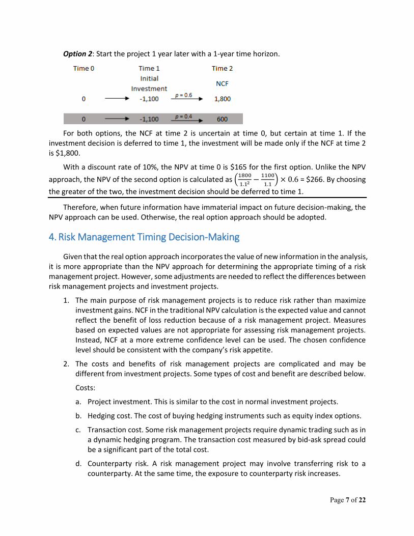
Option 2: Start the project 1 year later with a 1-year time horizon.

If the company wait for 1 year, the investment at time 1 is $1,100. The NCF of the second time period is still uncertain, as in Option 1.

With a discount rate of 10%, the NPV at time 0 is $165 for the first option and $83 for the second option. By choosing the greater of the two, the investment should start immediately.

However, the NPV approach does not reflect the impact of risk. It also assumes that there will be no additional information in the future that can affect the decision and the NPV of future investment.

On the other hand, the real option approach incorporates the value of future information in the decision-making process. Continuing with the NPV example and assuming that the NCF at time 2 will be known exactly at time 1, a better decision could be made given the new information. If the NCF of the second period is known to be $1,800 at time 1, the investment will be made. If the NCF is known to be $600, no investment will be made.

Example: Investment Timing Decision Using the Real Option Approach

Option 1: Start the project immediately with a 2-year time horizon.

of 22

Option 2: Start the project 1 year later with a 1-year time horizon.

For both options, the NCF at time 2 is uncertain at time 0, but certain at time 1. If the investment decision is deferred to time 1, the investment will be made only if the NCF at time 2 is $1,800.

With a discount rate of 10%, the NPV at time 0 is $165 for the first option. Unlike the NPV

approach, the NPV of the second option is calculated as (1800

1.12−

1100

1.1) × 0.6 = $266. By choosing

the greater of the two, the investment decision should be deferred to time 1.

Therefore, when future information have immaterial impact on future decision-making, the NPV approach can be used. Otherwise, the real option approach should be adopted.

4. Risk Management Timing Decision-Making

Given that the real option approach incorporates the value of new information in the analysis, it is more appropriate than the NPV approach for determining the appropriate timing of a risk management project. However, some adjustments are needed to reflect the differences between risk management projects and investment projects.

1. The main purpose of risk management projects is to reduce risk rather than maximize investment gains. NCF in the traditional NPV calculation is the expected value and cannot reflect the benefit of loss reduction because of a risk management project. Measures based on expected values are not appropriate for assessing risk management projects. Instead, NCF at a more extreme confidence level can be used. The chosen confidence level should be consistent with the company’s risk appetite.

2. The costs and benefits of risk management projects are complicated and may be different from investment projects. Some types of cost and benefit are described below.

Costs:

a. Project investment. This is similar to the cost in normal investment projects.

b. Hedging cost. The cost of buying hedging instruments such as equity index options.

c. Transaction cost. Some risk management projects require dynamic trading such as in a dynamic hedging program. The transaction cost measured by bid-ask spread could be a significant part of the total cost.

d. Counterparty risk. A risk management project may involve transferring risk to a counterparty. At the same time, the exposure to counterparty risk increases.

of 22

e. The loss of upside gains. A risk management project can reduce the risk but at the same time limit the upside potential. The loss of gains needs to be considered in project assessment.

Benefits:

a. At a given confidence level or in an extreme event, the loss reduction because of the risk management project such as an interest rate risk hedging program.

b. The potential benefit of a lower borrowing cost because of a higher credit rating. A risk management project may increase the rating on enterprise risk management which is a key component of credit risk assessment by rating agencies. The benefit can be quantified as the product of three factors: the probability of getting a higher credit rating, the contribution of the project, and the magnitude of borrowing cost reduction.

c. The potential benefit of lower cost of capital. If a risk management project can improve the capital adequacy and liquidity position of a company, the cost of raising additional capital in a normal economic environment will be lower. The benefit is the expected reduction in the financing cost.

d. The potential benefit of better decisions. For example, an investment in building a more advanced risk assessment platform such as the economic capital framework could help senior management make informed decisions. The benefit of the investment is the product of the decreased probability of making a wrong decision and the cost of a wrong decision.

Most of the cost and benefit items listed above require complex predicting using either historical experience or experts’ opinions.

3. The value of future information is necessary but difficult to quantify. To determine the optimal timing, the key is to evaluate how future information may help improve future decisions. For example, to hedge the equity risk in a future financial crisis, equity index put options can be bought either immediately or later. Assuming that the economy is in the expansion phase, the key value of future information is a better understanding of the time that the economy will go into a recession period. If future economic data indicate a prolonged economic expansion phase, it may be better to defer equity risk hedging.

4. Some risk management projects are divisible across time. For example, a hedging program can be implemented at several stages gradually till it is fully completed. Staged risk management decisions include not only the timing but also the amount of investment at each stage. The decision-making process is even more complicated and may require dynamic programming.

With these adjustments, different timing options can be compared based on the NPV after considering the value of future information. In sections 5 to 7, specific considerations are discussed regarding these adjustments for different decision problems.

of 22

5. Timing of Hedging Financial Risks

For companies with much free capital, adopting the contrarian approach in financial risk hedging may be a good idea. If the economy has stayed in the expansion cycle for a long period and the market has started worrying about market bubbles, it is a good time to mitigate the risk been taken before the hedging cost rises. After the economy stagnates for a continuing period of time and financial stimulus plans start to have some beneficial outcomes, it may not be a good timing to reduce the risk exposure due to the high cost. On the other hand, taking risk is more profitable as most market participants are looking for counterparties to transfer the risk.

For companies that are in a distressed situation but still have a pretty big chance of recovery, it may be better for them to only hedge short term earnings volatility to ease the panic of investors. Long term arrangement of risk transfer in difficult times may not be a wise decision. However, these companies may not have a choice at that time due to the pressure from the regulator, rating agencies, customers, and the public.

A key consideration in determining the appropriate timing of hedging financial risks is the future changes in economic conditions. In a situation where future economic situation is unclear, deferring the decision on financial risk hedging may buy decision maker some time to get a better view of future economic development and then make a more informed decision. In the following example, the company wants to hedge its exposure to equity risk but is also considering different timing options.

Example: Equity Risk Hedging

Insurance Company ABC sells VA products with a guaranteed minimum account value equal to 100% of paid premium. It has a large exposure to equity downside risk. The existing exposure is below the company’s risk tolerance. However, the company has a business expansion plan that needs extra capital. By hedging the equity risk, some required capital can be freed to support the business expansion plan.

The economy has been recovering from the 2008 financial crisis for 6 years. It is difficult to predict whether the economy will continue expanding or move slowly into another recession. To evaluate the timing options of hedging, the company needs to predict the change in market volatility which has a significant impact on the cost of hedging. The company plans to buy stock index put options so that it can hedge the minimum guarantee but not give up the potential upside. The higher the market volatility, the higher the cost of buying put options. The following graph shows the S&P 500 daily index and its volatility index from January 2, 1990 to November 11, 2015. Spikes of the VIX 2 are normally accompanied with material downward market movements. The correlation coefficient between the daily change in the index value and the daily change in the VIX is -71% over the study period.

2 VIX is a volatility index developed by the Chicago Board Options Exchange that tracks the implied volatility based

on the prices of options on the S&P 500 index.

of 22

Source: Yahoo! Finance

For the timing decision, an important question to answer is that given the current level of VIX, what the value of VIX will be in 1 month, 3 months, etc. If the VIX is likely to go down, the company may want to defer the hedging for lower cost of put options. If the VIX is likely to go up, the company may want to buy the put options immediately.

For simplicity, the only cost of the hedging program to be considered is the cost of put options. For the same reason, the price of put option is assumed to change only with volatility parameter across time. In practice, when considering timing options, other assumptions such as interest rate can also be assumed to be time variant.

The benefits of the hedging program include (a) the loss reduction if the stock index value falls below the exercise price; and (b) the saving of the cost of raising capital for the business expansion plan. Both the two benefits vary with future economic environment. In an economic expansion, the benefit of loss reduction is small but the saving of capital cost is large. In an economic recession, the benefit of loss reduction is large but the saving of capital cost is zero because the company is unlikely to have enough financial resources for the expansion.

Generally speaking, the current level of market volatility has a big impact on the timing decision.

1. In a low volatility situation (Low VIX), the cost of hedging is relatively low. It is likely that the hedging program should be implemented immediately.

2. In a high volatility situation (High VIX), the cost of hedging is high and the loss due to the bear market has already happened. In addition, the business expansion plan may need to be deferred due to stressed financial conditions. Therefore, it is likely the hedging program should be deferred.

3. In a medium volatility situation (Medium VIX), the timing decision becomes complicated.

of 22

If the economy is heading into recession, the cost of hedging is lower now than later. The benefit of hedging is likely to be realized in the near future. In this case, it is better to implement the hedging strategy immediately. If the economy will remain expanding, the cost of hedging is higher now than later and the benefit of hedging may not be realized in the near future. Because it is difficult to predict the future economic conditions, it may worth waiting for a certain period to get a clearer idea of the direction of the economy.

The table below lists the transition matrix of S&P 500 VIX with a period of 3 months based on the data from January 2, 1990 to November 11, 2015. In the low volatility range (VIX <20%), the VIX has a very high probability of staying in the low range. In the high volatility range (VIX> 30%), there is a high probability that the VIX will go down in the next 3 months. In the middle volatility range (VIX ϵ [20%, 30%]), VIX has a high chance to stay in the middle range or go down. But the chance of going up is not negligible.

3-month Transition Matrix of VIX (Jan. 1990 – Nov. 2015)

VIX <10% [10%, 20%) [20%, 30%) [30%, 40%) [40%, 50%) ≥50%

<10% 0.0% 100.0% 0.0% 0.0% 0.0% 0.0%

[10%, 20%) 0.3% 84.0% 12.6% 2.6% 0.5% 0.1%

[20%, 30%) 0.0% 29.5% 57.6% 9.7% 1.1% 2.1%

[30%, 40%) 0.0% 10.7% 68.5% 16.6% 3.4% 0.7%

[40%, 50%) 0.0% 0.0% 47.3% 39.3% 13.4% 0.0%

≥50% 0.0% 0.0% 1.8% 16.1% 71.4% 10.7%

Assuming that the current VIX is 25%, which is the average value in the middle range based on the experience data, the company is considering whether to implement the hedging program immediately or 3 months later. The company wants to hedge an equity risk exposure of $50 million for one year.

Option 1: Hedging immediately.

The cost of hedging is estimated to be $3.8 million with an interest rate of 4.5%, an implied volatility of 25%3 and a term of 1 year using the Black-Scholes formula for a European put option.

Based on the experience data, three real world scenarios are assumed at the end of one year:

3 The VIX is used as the implied volatility for simplicity. In reality, the implied volatility varies by option type (Call

or put), term of the option contract, and the level of exercise price (in-the-money/at-the-money/out-of-the-money

option).

of 22

Notes:

1. Three scenarios are assumed for the equity value at the end of one year. In the up scenario the equity value is $57.2 million with a probability of 33%. In the middle scenario, the equity value is $50.8 million with a probability of 49%. In the down scenario, the equity value is $41 million with a probability of 18%. The three scenarios represent the average equity values for the low, medium and high VIX scenarios, respectively. Both the equity values and the probabilities are derived from the historical data of S&P 500 Index and VIX from January 1990 to November 2015.

2. Only in the down scenario will the at-the-money equity put option be exercised. The payment is $9 million ($50 million – $41 million).

3. The hedging will release the required capital used to support equity risk. It is assumed that the company sets the required capital at a confidence level of 99.5%. Assuming the equity value

follows a lognormal distribution with = 7% and = 25%, the required capital is calculated as

the cost of capital rate × initial exposure × (1-0.5th percentile of lognormal (, )). The cost of capital rate is assumed to be 6%. Initial exposure is $50 million. The 0.5th percentile of lognormal (0.07, 0.25) is the left-tail 0.5% VaR. (1- 0.5th percentile) is the smallest loss in the worst 0.5% scenarios and is used to calculate the required capital to be freed. The reduced cost of capital is estimated to be $1.3 M.

The cost of Option 1 is $3.8 million at time 0. The benefit is $2.9 million at the end of one year, which is the sum of put option payment ($9M × 0.18 = $1.6M) and the reduced cost of capital ($1.3M). The return on investment (ROI)4 is -23% and the NPV with a hurdle rate of 10% is -$1.1 million. From the perspective of maximizing the investment gain, Option 1 is not a good option because of negative ROI and NPV. In practice, other benefits of the hedging may exist that could improve the NPV and ROI significantly. For example, a reduction in required capital could lead to an improved capital position and a credit rating upgrade which can reduce the borrowing cost. For simplicity, these potential benefits are not included in the example. The focus here is the comparison of the NPVs between different timing options.

4 Here ROI is the internal rate of return (IRR). It is the discount rate that makes the NPV equals to 0.

Time 0 12 Months

Cost of Put

Option

Equity

Value

Equity

Value 1Put Option

Payment 2Reduced Cost

of Capital 3

$57.2M 0 $1.3M

$3.8M $50M $50.8M 0 $1.3M

$41M $9M $1.3M

p = 0.49

of 22

Option 2: Deferring the hedging decision for 3 months.

The company also wants to consider delaying the hedging decision for 3 months. It has the following assumption of changes in the VIX in 3 months based on experience data.

Notes:

1. The VIX may drop to 18% with a probability of 29%, change to 24% with a probability of 58%, and go up to 39% with a probability of 13%. Both the VIX and probability are derived from the historical data of VIX from January 1990 to November 2015.

2. The cost of buying put option at the end of 3 months for each scenario is calculated with an interest rate of 4.5% and a term of 9 months. The exercise price is equal to the minimum of the equity index price at time 0 and the equity index price at the end of 3 months. In the Low VIX scenario (“up” scenario for equity price), the equity value is expected to be $53.3 million. The put option to be bought at the end of 3 months will have an exercise value of $50 million. In the medium VIX scenario (“medium” scenario for equity price), the equity value is expected to be $50.9 million, the exercise value of the put option will be $50 million. In the high VIX scenario (“down” scenario for equity price), the equity value is expected to be $44 million. The exercise value of the put option will be $44 million instead of $50 million. The cost of the in-the-money put option with an exercise value of $50 million is too high in the high VIX scenario.

The following scenarios of equity values at the end of one year, given the value at the end of three months are assumed:

Time 0 3 Months

Volatilty Volatility1Cost of Put

Option2

18% $1.2M

25% 24% $2.9M

39% $5.8M

p = 0.58

of 22

Using the same method as in Option 1, the benefit of hedging in each scenario (“up”, “middle”, or “down”) at the end of 3 months can be calculated. The results are listed in the following table.

Scenario Up Middle Down

NPV@10% 0.45 0.04 -5.20

ROI 70% 12% -96%

Probability 29% 58% 13%

Time Cash Flows

0 0 0 0

0.25 -1.20 -2.90 -5.80

1 1.78 3.16 0.51

Decision Hedge Hedge No

Both the up scenario and middle scenario have a positive NPV. In these two scenarios, hedging is likely to be implemented at the end of 3 months. In the down scenario, negative NPV indicates that the hedging strategy will not be implemented. The cost of the unhedged position in the down scenario is the loss caused by the equity value dropping below $50 million. It is calculated as below.

Time 0 3 Months 12 Months

Equity

Value

Equity

Value

Equity

Value

$58.1M

$52.1M

Up $43.7M

$53.3M

Middle $56.6M

$50M $50.9M $51.5M

Down $40.3M

$44M

$56M

$46.8M

$38.8M

p = 0.58p = 0.54

of 22

Cost of unhedged position in the down scenario = ($50M - $46.8M) × 0.65 + ($50M - $38.8M) × 0.1 = $3.2M.

The NPV of Option 2 at time zero is -$0.2 million, calculated as the weighted average of the values in three scenarios based on the chosen strategy. The weight is the probability of each scenario. The value is the NPV of the hedging strategy for the up and middle scenarios and the cost of unhedged position in the down scenario. It is much higher than the NPV of Option 1, which is -$1.1 million. Therefore, the company is better waiting for 3 months before making decisions on hedging implementation.

In this example, transition matrix based on experience data is used as one of many possible approaches. The history may not be a good indication of the future because of the persisting low interest rate environment that never happened before. Advanced predictive models adapted for the new economic regime can be used in practice. The trinomial tree can also be replaced by a stochastic model that considers thousands of scenarios.

In practice, threshold based decision mechanism can be designed for easy monitoring. For example, the middle scenario has a near-zero NPV. A possible simplified decision-making mechanism could be that if the VIX is no greater than 24%, which is the volatility in the middle scenario, hedging strategy will be implemented immediately. Otherwise, the decision will be deferred.

The approach used in the example above can be used for other projects such as deciding the optimal timing of raising capital. The cost of financing changes with economic environment as well. Raising additional capital during an economic expansion is less costly than during an economic recession. Incorporating economic cycles in the analysis can provide valuable information to decision-making regarding capital management.

6. Timing of Hedging Insurance Risks

Similar to the timing decision on hedging financial risks, the optimal timing of hedging insurance risks needs to consider the possible changes in costs and benefits in the future caused

Time 0 3 Months 12 Months

Equity

Value

Equity

Value

Equity

Value

$50M

Down

$44M

$56M

$46.8M

$38.8M

of 22

by changes in the market condition. In addition to the economic cycle, insurance cycle is an important consideration for hedging insurance risks.

Insurance cycle, a.k.a. the underwriting cycle, is the cyclical pattern of insurance prices and profits for the property and casualty insurance industry. A full cycle consists of two phases: soft market and hard market. A soft market is featured with increasing competition, relaxing underwriting rules, lower insurance price and profit. With a capacity constraint or a major catastrophic event, the market moves into a hard market. A hard market is featured with stringent underwriting, higher insurance price and improved profit. Meier and Outreville (2003) showed that the return on equity (ROE) of the U.S. P&C insurance industry has a material impact on the reinsurance price. A lower ROE indicates a higher reinsurance price. A higher reinsurance price could also indicate a higher level of hedging cost for insurance risk.

If the hedging is not immediately needed, the company can decide the most appropriate time for implementing the hedging. The cost of hedging is a major component in the timing decision. For example, a company wants to hedge its exposure to catastrophe risk by issuing catastrophe bonds. The market changed into a hard market one year ago. The company’s capital position is strong and does not need to reduce its risk exposure immediately. In this case, the company may consider the following factors for its timing decision.

1. When the market will move to a soft market? In a soft market, the cost of issuing catastrophe bonds will be lower. It might worth waiting if the hedging is a long-term plan. Some models are available to predict insurance cycles such as the regime-switching model proposed by Wang et al (2011).

2. The company could also take a staged approach by issuing a small portion of the total amount in a hard market and gradually increasing the amount of hedging as the market moves into a soft market.

3. When evaluating different timing options, the company needs to consider the potential loss caused by catastrophes during the period before hedging is in place.

Real option approach can be used in a similar way to the analysis of financial risk hedging. The value of new information is estimated using the insurance cycle modeling rather than the economic cycle modeling.

7. Timing of Risk Management Investment

Building new risk management functions is important but also expensive. Other important projects may also compete for limited resources. Unless the risk management investment is required immediately by regulators, it is helpful to study its optimal timing from an economic perspective.

The benefit of building new risk management functions are difficult to quantify. For example, building an economic capital (EC) framework can improve a company’s risk analysis capability, improve future risk decisions, and in the long term may contribute to a credit rating upgrade. Unlike the examples of hedging programs in the previous sections, most of the assessments could be quite subjective and few company-specific experience can be relied on. The timing

of 22

consideration is even more ambiguous. In practice, the timing is determined after the Board or senior management have made the decision to build the EC framework. The actual timing depends heavily on the availability of resources. Therefore, the optimization of timing for investment in the EC framework is not a scientific task. An example of high-level assessment of an EC project and its timing is given below.

Example: Investment in Building an EC Framework

Insurance Company ABC is considering building an EC framework and its applications to enhance the company’s risk management. The company has been using factor based approach to assess risk exposure and calculate risk charges. The EC framework will be a major enhancement of the risk analysis in the company. The company will also use EC as an additional measure for capital management and performance measurement. The project is expected to require an initial investment of $20 million. Annual cost is expected to be $2 million inflated by 3% each year. Company ABC is considering whether and when to make the investment.

The benefits that Company ABC is looking for are:

1. A contribution to the company’s enterprise risk management rating. The company plans to boost its credit rating in the medium term (3 to 5 years) from A+ to AA-. ERM rating is an important component of risk assessment by rating agencies. By using the EC framework in business decision-making, the company wants to improve its risk management practices.

2. The EC framework will be used to help improve business decision-making such as capital management, new business planning, risk optimization, and performance measurement. Risk adjusted return on economic capital will be used as a new measure. The benefit is measured by comparing the decision without the support of EC results and the decision with the support of EC results. The company had some successful capital management decisions and some unsuccessful ones in the past. If the EC framework was there, it may correct some wrong decisions but may also change some correct decisions. The net impact is seen as the benefit of the new project.

3. Company ABC has a business expansion plan that requires significant financing in the next 5 years. With the EC framework, the company hopes to reduce financing cost. The company plans to issue bonds and shares at the same time. If the credit rating is upgraded, the company could save about 10bps in terms of the cost of capital rate. The EC model can also help the company understand the amount of capital it needs to raise to remain the same level of capital adequacy. The additional information generated from the EC model may lead to a reduced level of required capital and therefore less capital cost. It may also lead to an increased level of capital to be raised. In this case, the future cost of capital raising or risk mitigation will be smaller as well after gaining a stronger capital position as indicated by the EC result.

As this is not a regulatory requirement, Company ABC does not have to build the EC framework immediately. Several considerations on the timing is under review.

1. The company wants to raise capital for the business expansion during an economic

of 22

expansion to control the cost. Therefore, it is ideal that the EC framework building can be finished before the capital raising and the future economic downturn. The economy has been recovering from the last financial crisis for 6 years. The economy may keep expanding or move into a recession. If the company starts the EC project now, it runs into the risk that the economy goes into a recession in the near future. The company will not implement the business expansion plan then and the benefit of the EC framework will be limited. In that case, the initial investment may be better used to improve the capital position rather than build the EC framework. On the other hand, if the company wait for half a year or one year, the direction of the economy could be clearer and the company may be able to make a more informed decision. For example, the Fed has implemented the near-zero interest rate (0 to 25 bps) policy for nearly 7 years. A series of increases in the Fed rate would indicate an expanding economy ahead. Keeping the rate unchanged or reducing it further would indicate a higher risk of economic recession. The Fed actively monitors the unemployment rate, inflation rate, and economic activities to decide the rate level. There have been many discussions on rate hiking in 2015. In a half year or one year, we may see a rate increase which raises the probability of a continuing economic expansion in the medium term. The company may decide to start the project immediately at that time. On the other hand, the average period of an economic cycle after World War II is 7 years. An economic recession is also a possible scenario. If we experience a level rate or a rate decrease in the next half year or one year, the probability of an economic recession will be higher. In that case, the company may decide to postpone the project.

2. The company does not have any experience on economic capital modeling and application. Without back testing and proper model validation, the EC result could be very sensitive to assumptions and misleading. In the 2008 financial crisis, some global insurance companies needed government bail out to survive although the economic capital result had showed that these companies had strong capital positions and affluent free capital to deploy. Before the investment, the company may want to gain additional knowledge and experience to better assess the benefits of the EC framework.

3. If the company wait for another 6 or 12 months for the EC project and then decide to build the EC framework, it may end up with an additional $10 million cost to achieve the target timeline of capital raising and business expansion. If interest rates are raised up during that period, the financing cost will be higher as well.

With a 10-year time horizon, the following high level estimates of the costs and benefits are used for the timing decision.

of 22

Option 1: Starting the project immediately.

Inflation Rate 3% NPV $0.03

Unit: $M Discount Rate 10% ROI 10%

Time Investment (1)

Benefit of Improved Decisions (2)

Benefit of Reduced Cost of Capital (3)

Expected NCF (4)

p=0.5 (2a) q=0.5 (2b) p=0.5 (3a) q=0.5 (3b)

0 20.0 -20.0

1 2.0 4.0 1.0 0.0 0.0 0.5

2 2.1 4.1 1.0 0.0 0.0 0.5

3 2.1 4.2 1.1 15.0 0.0 8.0

4 2.2 4.4 1.1 15.0 0.0 8.0

5 2.3 4.5 1.1 15.0 0.0 8.1

6 2.3 4.6 1.2 1.0 0.0 1.1

7 2.4 4.8 1.2 1.0 0.0 1.1

8 2.5 4.9 1.2 1.0 0.0 1.1

9 2.5 5.1 1.3 1.0 0.0 1.1

10 2.6 5.2 1.3 1.0 0.0 1.2

Notes:

(1). Investment: $20 million initial investment with an annual cost of $2 million growing by an inflation rate of 3%.

(2). Benefit of improved decisions: Based on the company’s current knowledge, the benefit of improved decisions has an even chance to be $4 million or $1 million in the first year, growing by the inflation rate annually.

(3). Benefit of reduced cost of capital: Because the direction of economic development is unclear now, the company expects two economic scenarios with equal chances. In the economic expansion scenario, the company will raise additional capital to implement the business expansion plan. The benefit of reduced cost will be realized from the 3rd year, with $15 million for 3 years, followed by $1 million till the end of the time horizon. In the economic recession scenario, the business expansion plan will be cancelled and no benefit will be gained.

(4). The NCF is calculated as (2a) × 0.5 + (2b) × 0.5 + (3a) × 0.5 + (3b) × 0.5 – (1). The ROI is 10%. With a hurdle rate of 10%, the NPV is $0.03 million.

of 22

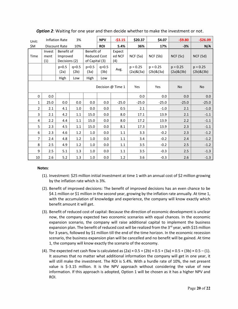
Option 2: Waiting for one year and then decide whether to make the investment or not.

Unit: $M

Inflation Rate 3% NPV -$3.15 $20.37 $4.07 -$9.80 -$26.09

Discount Rate 10% ROI 5.4% 36% 17% -3% N/A

Time Investment (1)

Benefit of Improved Decisions (2)

Benefit of Reduced Cost of Capital (3)

Expected NCF (4)

NCF (5a) NCF (5b) NCF (5c) NCF (5d)

p=0.5 (2a)

q=0.5 (2b)

p=0.5 (3a)

q=0.5 (3b)

Avg. p = 0.25 (2a)&(3a)

p = 0.25 (2b)&(3a)

p = 0.25 (2a)&(3b)

p = 0.25 (2b)&(3b)

High Low High Low

Decision @ Time 1 Yes Yes No No

0 0.0 0.0 0.0 0.0 0.0

1 25.0 0.0 0.0 0.0 0.0 -25.0 -25.0 -25.0 -25.0 -25.0

2 2.1 4.1 1.0 0.0 0.0 0.5 2.1 -1.0 2.1 -1.0

3 2.1 4.2 1.1 15.0 0.0 8.0 17.1 13.9 2.1 -1.1

4 2.2 4.4 1.1 15.0 0.0 8.0 17.2 13.9 2.2 -1.1

5 2.3 4.5 1.1 15.0 0.0 8.1 17.3 13.9 2.3 -1.1

6 2.3 4.6 1.2 1.0 0.0 1.1 3.3 -0.2 2.3 -1.2

7 2.4 4.8 1.2 1.0 0.0 1.1 3.4 -0.2 2.4 -1.2

8 2.5 4.9 1.2 1.0 0.0 1.1 3.5 -0.2 2.5 -1.2

9 2.5 5.1 1.3 1.0 0.0 1.1 3.5 -0.3 2.5 -1.3

10 2.6 5.2 1.3 1.0 0.0 1.2 3.6 -0.3 2.6 -1.3

Notes:

(1). Investment: $25 million initial investment at time 1 with an annual cost of $2 million growing by the inflation rate which is 3%.

(2). Benefit of improved decisions: The benefit of improved decisions has an even chance to be $4.1 million or $1 million in the second year, growing by the inflation rate annually. At time 1, with the accumulation of knowledge and experience, the company will know exactly which benefit amount it will get.

(3). Benefit of reduced cost of capital: Because the direction of economic development is unclear now, the company expected two economic scenarios with equal chances. In the economic expansion scenario, the company will raise additional capital to implement the business expansion plan. The benefit of reduced cost will be realized from the 3rd year, with $15 million for 3 years, followed by $1 million till the end of the time horizon. In the economic recession scenario, the business expansion plan will be cancelled and no benefit will be gained. At time 1, the company will know exactly the scenario of the economy.

(4). The expected net cash flow is calculated as (2a) × 0.5 + (2b) × 0.5 + (3a) × 0.5 + (3b) × 0.5 – (1). It assumes that no matter what additional information the company will get in one year, it will still make the investment. The ROI is 5.4%. With a hurdle rate of 10%, the net present value is $-3.15 million. It is the NPV approach without considering the value of new information. If this approach is adopted, Option 1 will be chosen as it has a higher NPV and ROI.

of 22

(5). Using the real option approach, at time 1, the company gets to choose whether to make the investment or not. (5a) to (5b) are four scenarios and the company will know exactly which scenario will play out. The NCF of each scenario is the sum of corresponding benefits deducted by the investment. For example, the NCF of (5a) = (2a) + (3a) – (1). Scenarios (5a) and (5b) will lead to a positive NPV. The investment will be made if (5a) or (5b) is expected at time 1. No investment will be made if (5c) and (5d) is realized. The aggregate NPV of Option 2 is $6.1 million (20.4 × 0.25 + 4.1 × 0.25). Compared to the NPV of Option 1, the company should wait 1 year before making the investment decision.

Scenario Benefit of Improved Decisions

Benefit of Reduced Cost of Capital

Probability Decision ROI NPV ($M)

4a High High 0.25 Yes 36% 20.4

4b Low High 0.25 Yes 17% 4.1

4c High Low 0.25 No -3% -9.8

4d Low Low 0.25 No N/A -26.1

Aggregate [(4a) and (4b) Only] $6.1

For simplicity, it is assumed that the company will know exactly the actual scenario at time 1 in this example. In reality, it is not realistic but the company may have a much better idea which scenario is most likely one. It can be reflected by assigning a different probability than 25% for each scenario.

The costs, benefits and the value of future new information vary from one risk management investment to another. They may not always be quantifiable and the uncertainty could be very high. Experts’ opinions are useful for choosing the best timing as well. For example, the company may not need 1 year extra time to better understand the benefit of improved decisions. Seeking the opinions of experts with relevant experience may shorten the knowledge gap.

8. Conclusion

The timing of a risk management project could have a material impact on the cost, such as the hedging cost of a hedging program or the cost of capital in a financing plan. Choosing the right timing of implementing a risk management strategy or starting an investment in new risk management functions is important.

Traditional approaches such as the NPV and real option approach used for investment decisions can be adjusted and used for timing decisions on risk management projects. The cost and benefit of a risk management project are different from a traditional investment. Risk management projects focus on more extreme scenarios than the expected cases.

Assessing the value of future new information and their impact on future decisions is the key

of 22

to timing decisions for risk management projects. The assessment usually requires comprehensive and complex analysis.

9. References

[1] Meier, Ursina B. and J. François Outreville, “The Reinsurance Price and the Insurance Cycle.” (2003) http://www.huebnergeneva.org/documents/Meier3.pdf

[2] Russo, J. Edward and Paul J. H. Schoemaker, “Decision Traps: Ten Barriers to Brilliant Decision-Making and How to Overcome Them.” (1990).

[3] Wang, Shaun S., John A. Major, Hucheng (Charles) Pan, and Jessica W. K. Leong, “U.S. Property-Casualty: Underwriting Cycle Modeling and Risk Benchmarks.” Variance, V5(2) (2011): 91-114.

http://www.variancejournal.org/issues/05-02/91.pdf

http://www.huebnergeneva.org/documents/Meier3.pdf

http://www.variancejournal.org/issues/05-02/91.pdf

the optimal timing of risk management - … · the optimal timing of risk management ... insurance...

Documents